Entropy production of soil hydrological processes and its

Earth Syst. Dynam., 2, 179–190, 2011www.earth-syst-dynam.net/2/179/2011/doi:10.5194/esd-2-179-2011© Author(s) 2011. CC Attribution 3.0 License.

Earth SystemDynamics

Entropy production of soil hydrological processes and itsmaximisation

P. Porada, A. Kleidon, and S. J. Schymanski

Max Planck Institute for Biogeochemistry, P.O. Box 10 01 64, 07701 Jena, Germany

Received: 17 December 2010 – Published in Earth Syst. Dynam. Discuss.: 28 January 2011Revised: 13 July 2011 – Accepted: 14 August 2011 – Published: 2 September 2011

Abstract. Hydrological processes are irreversible and pro-duce entropy. Hence, the framework of non-equilibrium ther-modynamics is used here to describe them mathematically.This means flows of water are written as functions of gra-dients in the gravitational and chemical potential of waterbetween two parts of the hydrological system. Such a frame-work facilitates a consistent thermodynamic representationof the hydrological processes in the model. Furthermore, itallows for the calculation of the entropy production associ-ated with a flow of water, which is proportional to the productof gradient and flow. Thus, an entropy budget of the hydro-logical cycle at the land surface is quantified, illustrating thecontribution of different processes to the overall entropy pro-duction. Moreover, the proposed Principle of Maximum En-tropy Production (MEP) can be applied to the model. Thismeans, unknown parameters can be determined by settingthem to values which lead to a maximisation of the entropyproduction in the model. The model used in this study isparametrised according to MEP and evaluated by means ofseveral observational datasets describing terrestrial fluxes ofwater and carbon. The model reproduces the data with goodaccuracy which is a promising result with regard to the appli-cation of MEP to hydrological processes at the land surface.

1 Introduction

The analysis and modelling of soil hydrological processeson a global scale is a challenging task, mostly due to in-teractions of the mechanisms involved combined with spa-tial heterogeneity at many scales. Although single processes(e.g. infiltration or bare soil evaporation) are well understood,a unifying quantitative framework to describe hydrological

Correspondence to:P. Porada([email protected])

behaviour at catchment or larger scales is still missing (Siva-palan, 2005). It is therefore in general not possible to makecorrect predictions about a certain catchment or region basedon a model that has been designed for another catchment.This paper presents an alternative approach to model hy-drological processes. Instead of describing each single pro-cess by a standard empirical theory, the framework of non-equilibrium thermodynamics is used. Thermodynamic meth-ods have already been used byEdlefsen and Anderson(1943)to characterise soil moisture relations and they are the theo-retical basis of common hydrological state variables, such asthe matric potential of soil water. Gradients in matric po-tential between two locations can then be used to quantifythe tendency of the water to move from high to low poten-tials, e.g. from wet to dry soil. Later,Leopold and Lang-bein (1962) introduced the concept of entropy productioninto soil hydrology, using the analogy of a thermodynamicheat engine. Similar to heat moving along a temperature gra-dient towards the cooler temperature, the authors formulatedrunoff as a function of the gradient in the gravitational po-tential of water, which results from topography. By flowingdownhill, the water moves from high to low gravitational po-tential, thereby converting potential energy of water into ki-netic energy which is then dissipated into heat by friction.The entropy production of runoff is then proportional to theproduct of the flow of water and the gradient in gravitationalpotential. It corresponds to the amount of heat generated bythe flow divided by temperature.

Given the basic concepts of water potential and entropyproduction associated with a flow of water, what is neces-sary to use thermodynamics as a unifying framework for thedescription of hydrological processes? The soil is a non-equilibrium open system where gradients in water potentialdrive flows of water. Assuming local thermodynamic equi-librium (Kondepudi and Prigogine, 1998), a chemical poten-tial of water can be calculated as a function of the watercontent in a sufficiently small part of the soil hydrological

Published by Copernicus Publications on behalf of the European Geosciences Union.

http://creativecommons.org/licenses/by/3.0/

180 P. Porada et al.: Entropy production in soil hydrology

system. All exchange flows of water can then be formulatedas functions of gradients in the combined chemical and grav-itational potential of water. In the following, these combinedpotentials will be denoted by the term “water potential” andthey will be expressed by the symbol for chemical poten-tial (µ, e.g. Eq.1). The implementation of the thermody-namic framework described above into a simple land surface-vegetation model is one main motivation for this paper.

Having formulated flows of water as functions of gradi-ents in water potential, it is straightforward to quantify anentropy budget of the most important soil hydrological pro-cesses. This can be used to illustrate the relative contribu-tions of different processes to the overall dissipation at theland surface.

Another advantage of a thermodynamic formulation of hy-drological processes is the possibility to apply the principleof Maximum Entropy Production (MEP) to the respectivemodels (Kleidon and Schymanski, 2008). This is explainedusing the example of root water uptake at the global scale.The flow of water from soil to roots is formulated as a linearfunction of the gradient between soil and root water poten-tial, with a proportionality constantc. The value ofc com-prises all factors affecting the speed of water movement atthe root-soil interface such as soil type, macropore density,root density, hydraulic conductivity, etc. which are highlyvariable at the global scale. In theory, the value ofc at acertain place at a certain time is then determined by all thesemeasurable soil and vegetation properties. However, the re-lation between these properties andc is so unpredictable atthe spatio-temporal scale of our model, thatc is characterisedby a very large range of values. This is also the reason to as-sume a linear relation between the flow and the gradient inwater potential, since it is the simplest model possible, giventhat not much is known about howc is related to soil andvegetation properties at the scale of this model. At steadystate, a maximum in the entropy production associated withroot water uptake then results from a trade-off between theflow and the gradient which is driving it: in the presence ofalternative pathways (e.g. runoff or bare soil evaporation),high values ofc lead to a strong dissipation of the gradientand consequently to a large flow at a small gradient (Schy-manski et al., 2009). Conversely, small values ofc lead to alarge gradient but a small flow. Since the entropy productionis proportional to the product of gradient and flow, it showsa maximum at intermediate values ofc. MEP predicts thatthe value ofc which leads to maximum entropy productionis the most probable one, given the model structure and forc-ing. For reviews about MEP seeMartyushev and Seleznev(2006); Ozawa et al.(2003).

MEP and other approaches dealing with the dissipation offree energy have been recently used in hydrology and ecol-ogy to predict various properties of land surface systems,ranging from the spatial distribution of biomass in semiaridregions (Schymanski et al., 2010) to preferential flow on hill-slopes (Zehe et al., 2010). The aim of the present paper is to

determine parameter values of a global land surface model(JESSY/SIMBA,Porada et al., 2010) by MEP. In a secondstep, the model output based on these parameter values iscompared with empirical data to test whether the MEP-basedprediction leads to realistic results.

This paper is structured as follows: Sect.2 contains a de-scription of the most important parts of the model used inthis study, followed by the model setup in Sect.3. In Sect.4,the results of this study are presented, including a parametri-sation of the model according to MEP, an entropy budget ofthe hydrological cycle at the land surface and an evaluationof the model performance. The paper closes with a discus-sion and an outlook.

2 Model description

The model used in this study simulates terrestrial biogeo-chemical processes in a simple way at the global scale. Itconsists of a soil model called JESSY (JEna Surface SYs-tem model) and a vegetation model, SIMBA (SIMulator ofBiospheric Aspects). JESSY and SIMBA use global grid-ded climate data as input to predict fluxes of carbon and wa-ter at the land surface, including evapotranspiration, runoffand Net Primary Productivity (NPP). Furthermore, reservoirssuch as soil water, biomass and soil carbon can be quantified.The models use a global rectangular grid with a resolution of2.8125 degrees (this corresponds to the T42 resolution).

JESSY and SIMBA are designed to run independently,which means that each of the models can be coupled to othermodels and they do not have to be run together. JESSY, forinstance, needs the value of the vegetation water potential tocompute root water uptake. This value can be provided byany vegetation model or it could be prescribed as a boundarycondition. This increases the applicability of the two modelsto biogeochemical questions.

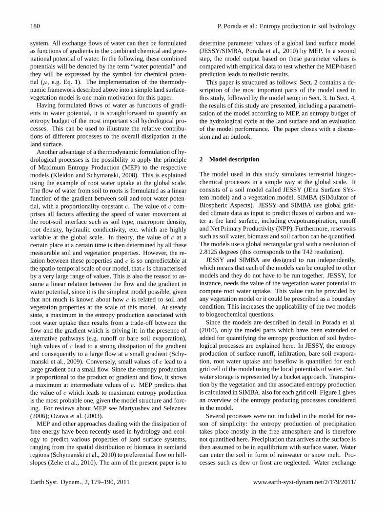
Since the models are described in detail inPorada et al.(2010), only the model parts which have been extended oradded for quantifying the entropy production of soil hydro-logical processes are explained here. In JESSY, the entropyproduction of surface runoff, infiltration, bare soil evapora-tion, root water uptake and baseflow is quantified for eachgrid cell of the model using the local potentials of water. Soilwater storage is represented by a bucket approach. Transpira-tion by the vegetation and the associated entropy productionis calculated in SIMBA, also for each grid cell. Figure1givesan overview of the entropy producing processes consideredin the model.

Several processes were not included in the model for rea-son of simplicity: the entropy production of precipitationtakes place mostly in the free atmosphere and is thereforenot quantified here. Precipitation that arrives at the surface isthen assumed to be in equilibrium with surface water. Watercan enter the soil in form of rainwater or snow melt. Pro-cesses such as dew or frost are neglected. Water exchange

Earth Syst. Dynam., 2, 179–190, 2011 www.earth-syst-dynam.net/2/179/2011/

P. Porada et al.: Entropy production in soil hydrology 181


Infiltrationfriction / immersion

Surface runofffriction

Baseflowfriction

µvegetation

µ: water potentialflows of water

µsoil Root water uptakefriction / immersion

Transpirationmixing

Bare soil evaporationmixing

µchannel

system boundary

River flowfriction

µsurface

subsystem boundary

µcoast

µocean

µsurface

µsoil

Precipitation@ µsurface

µatmosphere

µboundary layer

surroundings

Continentaldischarge@ µcoast

Evapotranspiration @ µboundary layer

Fig. 22.Overview of the flows of water (black text, regular) and theassociated entropy producing dissipative processes (red text, italics)quantified in JESSY and SIMBA. The grey shaded areas correspondto the surroundings of the system.

Fig. 1. Overview of the flows of water (black text, regular) and the associated entropy producing dissipative processes (red text, italics)quantified in JESSY and SIMBA. The grey shaded areas correspond to the surroundings of the system.

between the atmosphere and the surface water reservoirs(rivers, lakes) was not considered since the model does notcontain an explicit formulation of the river network. Hy-draulic redistribution cannot be properly described with thesimple bucket model used here and is therefore not included.Water flow from the river channel back to the soil does notseem to play a large role at the scale of a model grid cell andis neglected.

Note that all entropy production terms considered in themodel are due to processes within the system “land surface”.Since the system is assumed to be in steady state, the entropyproduced in the soil or the vegetation is completely exportedto the surroundings (Kondepudi and Prigogine, 1998, p. 387).Hence, the external entropy exchange flows are not consid-ered explicitly in our calculation. The assumption of steadystate also means that the reservoirs of the hydrological cy-cle at the land surface such as the soil water storage do notchange if averaged over long time periods (several decades).

A list of the most important model variables and param-eters can be found in Table A1. All model parameter val-ues are globally uniform, which is reasonable considering thesimplicity of the model. More complex parametrisations ofparts of the model such as different soil types, for instance,would represent an increase in complexity not matched bythe other parts of the model, e.g. the vegetation model. Fur-

thermore, the model is not very sensitive to the parametersoil type, probably due to its simplicity.

2.1 The potential of water in different parts of thehydrological system

The potential of water vapour in the atmospheric boundarylayer is written as (Kleidon and Schymanski, 2008):

µboundary layer= Rspec,vap Tair ln(8) + g z (1)

whereRspec,vap is the specific gas constant of water vapour,Tair is the temperature of the atmospheric boundary layer,8 is the relative humidity of the air,g is the gravitationalacceleration andz is the height above mean sea level.

Soil water potentialµsoil is formulated as the sum of themodified matric potential9M and the gravitational potentialof water in the soil (Kleidon and Schymanski, 2008). In gen-eral, both potentials vary with the heightz of the soil water:

µsoil(z) = 9M(z) + g z (2)

whereg is the gravitational acceleration. The gravitationalpotential increases linearly withz. The value of the matricpotential9M at heightz depends on the relative soil watercontent2soil(z) at that height. In unsaturated conditions, therelation between9M(z) and 2soil(z) is determined by the

www.earth-syst-dynam.net/2/179/2011/ Earth Syst. Dynam., 2, 179–190, 2011



equilibriumdistribution

soil moisture

water table

potential

matric potential

gravitational potential

µsoil

0

zc

bedrock

zs

0

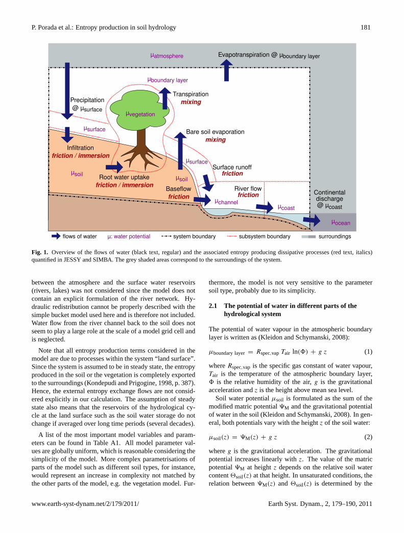
Fig. 23. Left: Equilibrium distribution of soil water inside thebucket,zs andzc correspond to the height of the surface and thechannel, respectively. Right: Soil water potentialµsoil as a functionof height.

Fig. 2. Left: equilibrium distribution of soil water inside the bucket,zs andzc correspond to the height of the surface and the channel,respectively. Right: soil water potentialµsoil as a function of height.

van-Genuchten soil water retention curve (van Genuchten,1980; Mualem, 1976). The value of9M(z) is negative anddecreases with decreasing saturation degree. This means thatthe more unsaturated the soil is, the more work has to beperformed to extract water from the soil matrix. The matricpotential is written as:

9M(z) = −g

αvg

((2soil(z)

2soil,max

)−

1mvg − 1

) 1nvg

(3)

2soil is defined as m3 extractable water m−3 soil. The rela-tion to saturationS is: S =2soil/2soil,max = (θ −θr)/(θs−θr)

where2soil,max is the relative extractable water content atsaturation.θ is the volumetric relative water content of thesoil in m3 water m−3 soil, θr is the residual relative soil wa-ter content andθs is the relative water content at saturationas defined invan Genuchten(1980). In the model used inthis studyθr and θs are set to values corresponding to thesoil type sandy loam (Carsel and Parrish, 1988) which can befound in Table A1.mvg, nvg, andαvg are the parameters ofthe van-Genuchten soil water retention curve and their valuescorrespond to the soil type sandy loam, too. Under saturatedconditions,9M(z) is replaced by the hydraulic head (Atkins,1998).

To obtain the value ofµsoil for the whole soil column,it is assumed that the water reaches a vertical equilibriumdistribution in each time step of the model. Consequently,the soil water potential is constant across the soil profile,µsoil(z) = const. This, however, requires a vertically non-uniform distribution of the water in the soil column (seeFig. 2). Each possible value ofµsoil(z) = const is then as-sociated with a different vertical equilibrium distribution ofwater. To assign the correct value ofµsoil to a given relativewater content of the soil2soil the equilibrium soil moisturedistribution whose integral is equal to the value of2soil iscalculated. The relationship ofµsoil and water content2soilis shown in Fig.3.


a)

b)

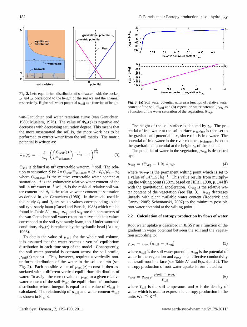
Fig. 24. a) Soil water potentialµsoil as a function of relative watercontent of the soil,Θsoil and b) vegetation water potentialµveg asa function of the water saturation of the vegetation,Θveg.

Fig. 3. (a)Soil water potentialµsoil as a function of relative watercontent of the soil,2soil and(b) vegetation water potentialµveg asa function of the water saturation of the vegetation,2veg.

The height of the soil surface is denoted byzs. The po-tential of free water at the soil surfaceµsurfaceis then set tothe gravitational potential atzs since rain is free water. Thepotential of free water in the river channel,µchannel, is set tothe gravitational potential at the heightzc of the channel.

The potential of water in the vegetation,µveg is describedby:

µveg = (2veg − 1.0) 9PWP (4)

where9PWP is the permanent wilting point which is set toa value of 1471.5 J kg−1. This value results from multiply-ing the wilting point (150 m, based onHillel , 1998, p. 144 ff)with the gravitational acceleration.2veg is the relative wa-ter content of the vegetation (see Fig.3). µveg decreaseslinearly with plant available water content (Roderick andCanny, 2005; Schymanski, 2007) to the minimum possibleroot water potential at the wilting point.

2.2 Calculation of entropy production by flows of water

Root water uptake is described in JESSY as a function of thegradient in water potential between the soil and the vegeta-tion according to:

qroot = croot(µsoil − µveg

)(5)

whereµsoil is the soil water potential,µveg is the potential ofwater in the vegetation andcroot is an effective conductivityat the soil-root interface (see Table A1 and Eqs.4 and2). Theentropy production of root water uptake is formulated as:

σroot = qroot ρµsoil − µveg

Tsoil(6)

whereTsoil is the soil temperature andρ is the density ofwater which is used to express the entropy production in theunits W m−2 K−1.



Baseflow is expressed as:

qbase = cbase(µsoil − µchannel) (7)

whereµchannel is the potential of water in the river channelandcbasecorresponds to the effective conductivity of the in-terface between the soil and channel. The entropy productionof baseflow is calculated as:

σbase = qbaseρµsoil − µchannel

Tsoil(8)

Bare soil evaporationqevapand transpirationqtransare cal-culated by the minimum of atmospheric demandqepot andthe amount of water which is available for evaporation fromthe soil and the vegetation during a day:

qevap = min

(qepot,

2soil 1S

1t

)(9)

qtrans = min

(qepot,

2veg 1V

1t+ qroot

)(10)

1S and1V are the “bucket depths” of soil and vegetation,respectively, and1t is the model time step which is set to aday. The demandqepot is quantified by an equilibrium evap-oration approach (McNaughton and Jarvis, 1983):

qepot =

(dsdT

dsdT

+ γfnet,0

)/λ (11)

withds

dT=

epvp1

zTpvp2 + zT pvp1 pvp2 pvp3(

pvp2 + zT)2 ρ

wherezT corresponds to (surface temperature in K – melt-ing temperature of water),fnet,0 is net radiation andds

dTis

the slope of the saturation vapour pressure versus tempera-ture relationship. The values of the parametersλ, pvp1, pvp2,pvp3, ρ andγ can be found in Table A1. To account for thedecrease in hydraulic conductivity at lower soil water con-tents, bare soil evaporation takes place only as long as thedifference between the maximum relative soil water contentand the actual one is smaller than 0.01. This value is chosensuch that, assuming a vertical equilibrium soil water distri-bution, the decrease in hydraulic conductivity at the top ofthe soil column is approximately 2 orders of magnitude (vanGenuchten, 1980). Since bare soil evaporation is small onvegetated surfaces, it is constrained to the fraction of baresoil in each grid cell. The entropy production of bare soilevaporation and transpiration is written as:

σevap = qevapρµsoil − µboundary layer

Tsurf(12)

σtrans = qtransρµveg − µboundary layer

Tsurf(13)

whereµboundary layeris the water vapour potential of the at-mospheric boundary layer andTsurf is the surface tempera-ture.

Surface runoff is described as saturation excess flow andis consequently controlled by the bucket size (see Table A1).The entropy production of surface runoff is then calculatedas:

σsurf = qsurf ρµsurface− µchannel

Tsurf(14)

whereµsurfaceandµchannelare used because free water flowsfrom the soil surface into the nearest river channel. The en-tropy production of the river dischargeqriver into the oceans,which consists of water from surface runoff and baseflow, isthen written as:

σriver = (qsurf + qbase) ρµchannel− µmsl

Tsurf(15)

whereµmsl corresponds to the potential of free water at meansea level, which is set to zero. Since the gradientsµsurface−

µchannelandµchannel−µmsl are constant, bothσsurf andσrivervary only with the flow rate.

Additionally, entropy is produced during the infiltration ofwater into the soil, which is formulated as:

σinf = (qrain − qsurf) ρµsurface− µsoil

Tsoil(16)

where qrain − qsurf is the amount of infiltrated water andµsurface−µsoil is the gradient between free water at the sur-face and bound water in the soil.

3 Model setup

JESSY and SIMBA are run on a global rectangular T42 grid(2.8125 degree resolution) with a climate data set (1971 to2006; Sheffield et al., 2006) that consists of shortwave ra-diation, downwelling longwave radiation, precipitation, av-erage temperature and minimum temperature at 2 m heighton a daily basis. Terrestrial longwave radiation and relativehumidity are derived from these variables (seePorada et al.,2010for further information). The model is run until all vari-ables are in a dynamic steady state. The model output is thenobtained by averaging over the last 10 yr of the simulation.

3.1 Observational datasets to test the model

JESSY and SIMBA are evaluated by comparing the modeloutput to datasets containing runoff, evapotranspiration, NetPrimary Productivity (NPP) and soil carbon. This methodhas already been used to evaluate the basic version of themodel (Porada et al., 2010).

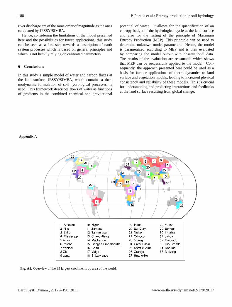
In a first test, runoff output from JESSY is compared toriver basin discharge data from the 35 largest catchments byarea of the world. A basin mask fromVorosmarty et al.(2000) is used to identify the model grid cells contributing



to a certain basin. The discharge data is taken fromDai andTrenberth(2002). An overview of the basins can be found inFig. A1.

In a second test, modelled evapotranspiration for each gridcell is compared with the one predicted by the empiricalBudyko curve (Budyko, 1974). The Budyko-curve estimatesevapotranspiration as a function of a climate index, whichis calculated from net radiation and precipitation. These aretaken from the climate input dataset. The climate index isthen calculated for each of the 35 largest river basins as afunction of the mean net radiation and precipitation over thebasin.

In a third test, the NPP and soil carbon content predictedby SIMBA is compared against global datasets. NPP-data isprovided byCramer et al.(1999) and includes the mean ofthe NPP-estimates of 17 different vegetation models. In thisway, the coupled JESSY/SIMBA model can be compared toother recent global vegetation models. Soil carbon estimatesfor the first meter of the soil column are taken fromIGBP-DIS (1998). The comparison is performed using latitudinalprofiles of NPP and soil carbon.

3.2 Determining the MEP-state of root water uptakeand baseflow

JESSY and SIMBA contain several unknown parameters,which had to be tuned previously (Porada et al., 2010). In thisstudy, two influential parameters,croot andcbase(see Eqs.6and8 and Table A1) are instead determined by MEP. Thismeans they are set to values which lead to a maximisation ofthe entropy production of the flows they control, namely rootwater uptake and baseflow. Since all model parameters areglobal, we maximise the global entropy production of oneflow, meaning the sum of all model grid cells, to determinethe associated parameter.

Maximising the entropy production of both root water up-take and baseflow requires an iterative approach, since thevalue of one parameter, e.g.cbase, may affect the MEP-statewith respect to the other parameter, e.g.croot, sincecbasede-termines a boundary condition for root water uptake. Hence,a stepwise approach is chosen to find the MEP-states of rootwater uptake and baseflow: first,cbaseis set to a fixed valueand the MEP-state of root water uptake is determined byvarying croot over several orders of magnitude (see Fig.4).Then,cbaseis set to another value and another MEP-state ofroot water uptake is determined. Thus, an MEP-value ofcrootis assigned to each value ofcbase. Finally, the pair ofcbaseandcroot which corresponds to an MEP-state of baseflow isselected (see Fig.4). This is then used for parametrising themodel and evaluating it by comparison with the observationaldata mentioned in Sect.3.1.

Table 1. Global land surface mean values of entropy productionaveraged over 10 yr of simulation with the JESSY/SIMBA modelwhich is parametrised according to MEP.

Hydrological process Entropy production Flow of waterin mW m−2 K−1 in km3 yr−1

Transpiration 2.4 74 682River discharge 1.1E-1 27 786Root water uptake 7.9E-2 74 624Infiltration 5.1E-2 91 415Evaporation 4.5E-4 21Baseflow 6.8E-5 16 814Surface runoff 9.1E-8 10 972

4 Results

By varying the two unknown model parameterscroot andcbase, the values corresponding to maximum entropy produc-tion of the flows root water uptake and baseflow are deter-mined (see Sect.3.2). These arecroot = 3.5E-11 s m−1 andcbase= 8.6E-9 s m−1 (see Fig.4). The model output obtainedby this parametrisation is then evaluated.

4.1 Model evaluation

To evaluate JESSY and SIMBA, the model output is com-pared to observational data described in Sect.3.1. All vari-ables contained in the datasets are affected by the parameterscroot andcbase that are optimised according to MEP. Whilerunoff and evapotranspiration are directly controlled by rootwater uptake and baseflow, NPP and soil carbon are influ-enced through the effect of root water uptake on the produc-tivity of vegetation. The results of the evaluation are shownin Fig. 5.

The model output shows reasonable agreement with ob-servational data. Both general patterns and absolute val-ues of runoff, evapotranspiration, NPP and soil carbon pre-dicted by the model are close to observations. Consideringthe Budyko-curve, modelled runoff in the northern temper-ate regions seems to be slightly too high. In comparison withrunoff data, however, the model seems to slightly underes-timate runoff in these regions. A possible reason to explainboth mismatches is underestimation of precipitation in themodel input data of the northern regions, as discussed inPo-rada et al.(2010).

4.2 Entropy budget of soil hydrological processes

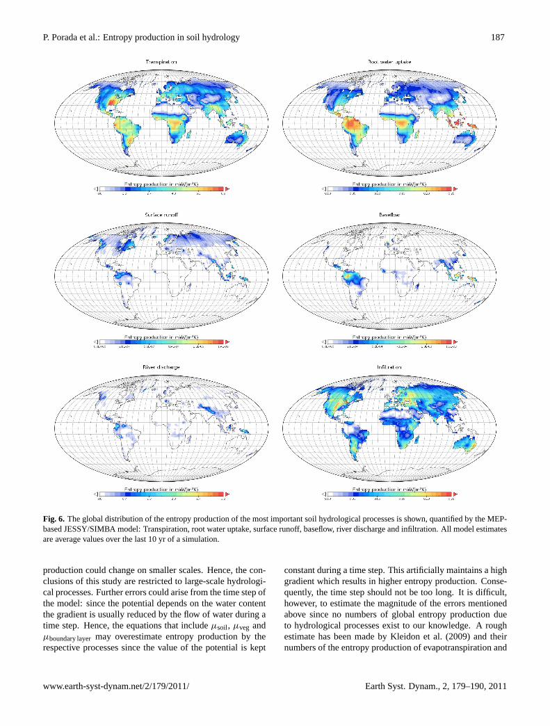
The results of the entropy budget of the hydrological cycle(Eqs.6 to 16) are shown in Fig.6 and in Table1. Note thedifferent scale ranges below each plot.

It can be seen that the entropy production due to transpi-ration dominates over other processes. The reason for this




croot cbase croot cbase

a) b)σrootσbase

1e-10

1e-09

1e-08

1e-07

1e-12

1e-11

1e-10

0

5e-05

0.0001

0.00015

0.0002

0.00025

0.0003

0

5e-05

0.0001

0.00015

0.0002

0.00025

0.0003

1e-10

1e-09

1e-08

1e-07

1e-12

1e-11

1e-10

00.010.020.030.040.050.060.070.080.09

0

0.01

0.02

0.03

0.04

0.05

0.06

0.07

0.08

0.09

Fig. 25. Entropy production of(a) baseflow and(b) root water up-take as a function of the two model parameterscbase andcroot. Thecombined MEP-state of baseflow and root water uptake lies at theintersection of the two “ridges” in(a) and (b), the correspondingvalues can be found in Table A.

Fig. 4. Entropy production of(a) baseflow and(b) root water uptake as a function of the two model parameterscbaseandcroot. The combinedMEP-state of baseflow and root water uptake lies at the intersection of the two “ridges” in(a) and(b), the corresponding values can be foundin Table A1.

is the large share of transpiration on the global water bal-ance combined with a strong gradient between vegetationand atmosphere. The latter also leads to a relatively highentropy production of bare soil evaporation compared to thesmall contribution of evaporation to the water balance (3 or-ders of magnitude smaller than other flows). The gradientsassociated with root water uptake and infiltration are muchsmaller, thereby leading to smaller values of the correspond-ing entropy production. While baseflow and surface runoffcontribute little to the entropy budget due to the very smallgradients in water potential associated with these processes,river discharge results in a relatively high entropy production,especially in mountainous regions characterised by high po-tential energy of water and high runoff.

5 Discussion

Non-equilibrium thermodynamics provides an additionalconstraint for the formulation of soil hydrological processes,which is usually not considered explicitly. Flows of waterare not only constrained by the mass balance, but they arealso driven by gradients in water potential between two loca-tions. The formulation of flows and gradients then directlyleads to the quantification of the entropy production of hy-drological processes. The entropy production characterisesthe irreversibility of these processes. This is illustrated inTable1: although root water uptake is of the same order ofmagnitude as baseflow, it is much more irreversible due tothe strong gradient in water potential between soil and atmo-sphere.

Apart from extending the theoretical basis of a hydrolog-ical model, the thermodynamic approach also makes possi-ble the testing of the Principle of Maximum Entropy Produc-tion (MEP). By applying MEP to the JESSY/SIMBA model,the values of two unknown model parameters that otherwisewould have to be tuned can be determined. In spite of thesimplicity of the model, the output of the MEP-parametrised

JESSY/SIMBA agrees well with observational data. Thissuggests that MEP can be used in this case to determine un-known parameter values instead of tuning them. In the scopeof behavioral modeling (Schaefli et al., 2011), this means thatMEP can be used as an organising principle in soil hydrologyat the global scale. The identification of organising principlessuch as MEP potentially plays a large role for improving hy-drological models, since these principles are assumed to begenerally valid and independent of changes in the forcing orin the structure of the system. Using a model as a tool toidentify the underlying organising principles thus representsa new approach to modelling hydrological processes and analternative to parameter tuning.

The reason why deriving model parameter values by MEPleads to realistic predictions is still a matter of discussion.One possible explanation could be that MEP is a physicalprinciple and systems “vary” their properties (expressed byparameters such ascroot andcbase) to achieve maximum en-tropy production. Alternatively, MEP can be interpretedas an algorithm to objectively “guess” some outcomes of amodel given the information contained in that model. Henceunknown parameters such ascroot andcbasecan be derivedsince the remaining model structure is sufficient to correctlyrepresent all important processes (Dewar, 2009).

Although some of the soil hydrological processes in theJESSY/SIMBA model can be parametrised by MEP, otherparts of the model still need to be reformulated using a ther-modynamic approach. Soil water, for instance, is assumed toreach a vertical equilibrium distribution in each time step ofthe model. This may not be possible in case vertical gradi-ents in soil water potential are insufficient to drive a strongwater movement towards equilibrium. Since a bucket modelis not able to represent vertical gradients in water potential,a layered model is needed here. Varying the conductivitiesbetween the layers, the flow of water through the soil couldthen be determined by MEP. Furthermore, evapotranspirationshould be written as a function of the gradient in relative hu-midity instead of using the minimum of supply and demand




1e-10

1e-09

1e-08

1e-07

1e-10 1e-09 1e-08 1e-07

Da

ta f

rom

35

la

rge

st

riv

er

ba

sin

s [

m/s

]

Model output from 35 largest river basins [m/s]

0

0.2

0.4

0.6

0.8

1

1.2

0 0.5 1 1.5 2

ET

/ E

po

t

P / Epot

a) b)

c) d)

P / Epot

ET

/ E

po

t

Model output from 35 largest river basins [m/s]

Data

fro

m 3

5 larg

est

river

bas

ins

[m

/s]

NP

P in

[kg

/m²/

yr]

Latitude

So

il C

arb

on

in

[kg

/m²]

Latitude

Fig. 26. (a)Modelled evapotranspiration averaged over a basin plot-ted against the theoretical Budyko-curve (magenta, dashed) for the35 world’s largest river basins.(b) Scatterplot of modelled runoffand measured runoff for the 35 largest river basins of the world.• corresponds to humid tropical,� humid subtropical,⊡ temperate,> cold continental and× (semi) arid climate regions.(c) Latitu-dinal pattern of modelled NPP (blue, solid) and the mean NPP of17 global vegetation models (magenta, dashed) latitudinal pattern ofmodelled (blue, solid) and measured soil carbon (magenta, dashed),both accumulated over the first meter of the soil. All shown modelestimates are derived from a MEP-based parametrisation. They areaverage values over the last 10 years of a simulation.

Fig. 5. (a) Modelled evapotranspiration averaged over a basin plotted against the theoretical Budyko-curve (magenta, dashed) for the35 world’s largest river basins.(b) Scatterplot of modelled runoff and measured runoff for the 35 largest river basins of the world.• corre-sponds to humid tropical,� humid subtropical,� temperate,> cold continental and× (semi) arid climate regions.(c) Latitudinal pattern ofmodelled NPP (blue, solid) and the mean NPP of 17 global vegetation models (magenta, dashed) latitudinal pattern of modelled (blue, solid)and measured soil carbon (magenta, dashed), both accumulated over the first meter of the soil. All shown model estimates are derived froma MEP-based parametrisation. They are average values over the last 10 yr of a simulation.

(see Eq.11). In the current implementation, this gradient isrepresented only indirectly by the saturation vapour pressureversus temperature relationshipds

dT. Not only flows of water,

but also carbon fluxes could be described in thermodynamicterms. MEP could be useful here since the parametrisationof diverse vegetation is difficult and often arbitrary. More-over, additional entropy producing hydrological processes atthe land surface could be included in the model. Amongthese are heat diffusion associated with temperature changesof soil water, irreversible chemical reactions of water withother substances within the soil and physical transformationsof the soil, including frost heaving and soil erosion.

Errors concerning the quantification of the entropy pro-duction in the model can result from the underestimation ofspatial and temporal variability due to the resolution of themodel. This means that spatial gradients in water potentialor temporal variability of rainfall, for instance, are not cap-tured by the mean values used for a grid cell. Since thesegradients could contribute to further entropy production, av-eraging might lead to underestimation of the entropy pro-duced. Another drawback of the relatively coarse resolu-tion of the model is the fact, that small-scale hydrologicalprocesses such as interflow are not considered. It shouldbe pointed out here that the relative importance of the dif-ferent hydrological processes and their associated entropy




Fig. 27. The global distribution of the entropy production of themost important soil hydrological processes is shown, quantified bythe MEP-based JESSY/SIMBA model: Transpiration, root wateruptake, surface runoff, baseflow, river discharge and infiltration.Allmodel estimates are average values over the last 10 years of a sim-ulation.

Fig. 6. The global distribution of the entropy production of the most important soil hydrological processes is shown, quantified by the MEP-based JESSY/SIMBA model: Transpiration, root water uptake, surface runoff, baseflow, river discharge and infiltration. All model estimatesare average values over the last 10 yr of a simulation.

production could change on smaller scales. Hence, the con-clusions of this study are restricted to large-scale hydrologi-cal processes. Further errors could arise from the time step ofthe model: since the potential depends on the water contentthe gradient is usually reduced by the flow of water during atime step. Hence, the equations that includeµsoil, µveg andµboundary layermay overestimate entropy production by therespective processes since the value of the potential is kept

constant during a time step. This artificially maintains a highgradient which results in higher entropy production. Conse-quently, the time step should not be too long. It is difficult,however, to estimate the magnitude of the errors mentionedabove since no numbers of global entropy production dueto hydrological processes exist to our knowledge. A roughestimate has been made byKleidon et al.(2009) and theirnumbers of the entropy production of evapotranspiration and



river discharge are of the same order of magnitude as the onescalculated by JESSY/SIMBA.

Hence, considering the limitations of the model presentedhere and the possibilities for future applications, this studycan be seen as a first step towards a description of earthsystem processes which is based on general principles andwhich is not heavily relying on calibrated parameters.

6 Conclusions

In this study a simple model of water and carbon fluxes atthe land surface, JESSY/SIMBA, which contains a ther-modynamic formulation of soil hydrological processes, isused. This framework describes flows of water as functionsof gradients in the combined chemical and gravitational

potential of water. It allows for the quantification of anentropy budget of the hydrological cycle at the land surfaceand also for the testing of the principle of MaximumEntropy Production (MEP). This principle can be used todetermine unknown model parameters. Hence, the modelis parametrised according to MEP and is then evaluatedby comparing the model output with observational data.The results of the evaluation are reasonable which showsthat MEP can be successfully applied to the model. Con-sequently, the approach presented here could be used as abasis for further applications of thermodynamics to landsurface and vegetation models, leading to increased physicalconsistency and reliability of these models. This is crucialfor understanding and predicting interactions and feedbacksat the land surface resulting from global change.

Appendix A


Appendix B

Overview of river basins.

Fig. B1. Overview of the 35 largest catchments by area of the world.

Fig. A1. Overview of the 35 largest catchments by area of the world.



Table A1. Description of model variables and parameters.

Symbol Description Value Units

pools 2veg relative vegetation water content2soil relative soil water contentCsoil organic carbon in soil kg C m−2

states Tsoil soil temperature KTsurf surface temperature KTair air temperature Kµboundary layer water vapour potential of atmospheric boundary layer J kg−1µveg vegetation water potential J kg−1µsoil soil water potential J kg−1µchannel potential of water in a river channel J kg−1µsurface potential of rain at surface J kg−18 relative humidity

rates qrain rainfall m s−1

qroot root water uptake m s−1

qbase baseflow m s−1

qtrans transpiration m s−1

qevap evaporation m s−1

qsurf surface runoff m s−1

qriver river discharge m s−1

NPP Net Primary Productivity kg C m−2 yr−1

σevap entropy production of evaporation W m−2 K−1

σtrans entropy production of transpiration W m−2 K−1

σroot entropy production of root water uptake W m−2 K−1

σbase entropy production of baseflow W m−2 K−1

σsurf entropy production of surface runoff W m−2 K−1

σriver entropy production of river discharge W m−2 K−1

σinf entropy production of infiltration W m−2 K−1

parameters g gravitational acceleration 9.81 m s−2

RV gas constant of water vapour 461.5 J kg−1 K−1

λ latent heat of vaporization 2.45E6 J kg−1

γ psychometric constant 65.0 Pa K−1

pvp1 parameter to calculate vapour pressure 17.269pvp2 parameter to calculate vapour pressure 237.3 Kpvp3 parameter to calculate vapour pressure 610.8 Paρ density of water 1000.0 kg m−3

z height above mean sea level mzs height of the soil surface above sea level mzc height of the channel above sea level zs−1.0 m1S depth of the soil bucket zs−zc m1V depth of the vegetation bucket 1.0 mcroot effective conductivity at soil-root interface 3.5E-11 s m−1

cbase effective conductivity at soil-channel interface 8.6E-9 s m−1

θr residual relative soil water content 0.065 (sandy loam)θs relative soil water content at saturation 0.41 (sandy loam)αvg van Genuchten parameterα 7.5 (sandy loam)nvg van Genuchten parametern 1.89 (sandy loam)mvg van Genuchten parameterm 0.47 (sandy loam)2soil,max relative extractable soil water content at saturation 0.3459PWP permanent wilting point 1471.5 J kg−1



Acknowledgements.The authors are thankful to Fabian Gansfor useful discussions about the topic. We thank the HelmholtzAlliance “Planetary Evolution and Life” for funding and twoanonymous reviewers for helpful comments.

Edited by: R. Niven

The service charges for this open access publicationhave been covered by the Max Planck Society.

References

Atkins, P. W.: Physical Chemistry, 6th Edn., Oxford UniversityPress, Oxford, 1998.

Budyko, M.: Climate and life, Academic Press, New York, 1974.Carsel, R. F. and Parrish, R. S.: Developing Joint Probability Dis-

tributions of Soil Water Retention Characteristics, Water Resour.Res., 24, 755–769,doi:10.1029/WR024i005p00755, 1988.

Cramer, W., Kicklighter, D. W., Bondeau, A., Moore III, B.,Churkina, G., Nemry, B., Ruimy, A., and Schloss, A.: Com-paring global models of terrestrial Net Primary Productiv-ity (NPP): overview and key results, Global Change Biol., 5, 1–15,doi:10.1046/j.1365-2486.1999.00009.x, 1999.

Dai, A. and Trenberth, K. E.: Estimates of Freshwater Dis-charge from Continents: Latitudinal and Seasonal Vari-ations, J. Hydrometeorol., 3, 660–687,doi:10.1175/1525-7541(2002)003<0660:EOFDFC>2.0.CO;2, 2002.

Dewar, R. C.: Maximum Entropy Production as an Inference Al-gorithm that Translates Physical Assumptions into MacroscopicPredictions: Dont Shoot the Messenger, Entropy, 11, 931–944,doi:10.3390/e11040931, 2009.

Edlefsen, N. E. and Anderson, A. B. C.: Thermodynamics of SoilMoisture, Hilgardia, 15, 31–298, 1943.

Hillel, D.: Environmental Soil Physics, Academic Press, 1998.IGBP-DIS: SoilData(V.0), A program for creating global soil-

property databases, IGBP Global Soils Data Task, France, 1998.Kleidon, A. and Schymanski, S.: Thermodynamics and optimality

of the water budget on land: A review, Geophys. Res. Lett., 35,L20404,doi:10.1029/2008GL035393, 2008.

Kleidon, A., Schymanski, S. J., and Stieglitz, M.: Thermodynam-ics, Irreversibility, and Optimality in Land Surface Hydrology,in: Bioclimatology and Natural Hazards, edited by: Strelcova,K., Matyas, C., Kleidon, A., Lapin, M., Matejka, F., Blazenec,M., Skvarenina, J., and Holecy, J., Springer, Berlin, Germany,107–118,doi:10.1007/978-1-4020-8876-69, 2009.

Kondepudi, D. and Prigogine, I.: Modern thermodynamics – fromheat engines to dissipative structures, Wiley, Chichester, 1998.

Leopold, L. B. and Langbein, W. L.: The concept of entropy inlandscape evolution, US Geol. Surv. Prof. Pap., 500-A, 20, 1962.

Martyushev, L. M. and Seleznev, V. D.: Maximum entropy produc-tion principle in physics, chemistry and biology, Phys. Rep., 426,1–45,doi:10.1016/j.physrep.2005.12.001, 2006.

McNaughton, K. G. and Jarvis, P. G.: Predicting effects of vegeta-tion changes on transpiration and evaporation, in: Water Deficitsand Plant Growth, edited by: Kozlowski, T. L., Academic Press,New York, 7, 1–47, 1983.

Mualem, Y.: A new model for predicting the hydraulic conductivityof unsaturated porous media, Water Resour. Res., 12, 513–522,doi:10.1029/WR012i003p00513, 1976.

Ozawa, H., Ohmura, A., Lorenz, R. D., and Pujol, T.: The secondlaw of thermodynamics and the global climate system – a reviewof the maximum entropy production principle, Rev. Geophys.,41, 1018,doi:10.1029/WR012i003p00513, 2003.

Porada, P., Arens, S., Buendıa, C., Gans, F., Schymanski, S. J.,and Kleidon, A.: A simple global land surface model for bio-geochemical studies, Technical Reports, Max-Planck-Institut furBiogeochemie, Jena, Germany, 18, 2010.

Roderick, M. L. and Canny, M. J.: A mechanical interpretationof pressure chamber measurements – what does the strengthof the squeeze tell us?, Plant Physiol. Biochem., 43, 323–336,doi:10.1016/j.plaphy.2005.02.014, 2005.

Schaefli, B., Harman, C. J., Sivapalan, M., and Schymanski, S. J.:HESS Opinions: Hydrologic predictions in a changing environ-ment: behavioral modeling, Hydrol. Earth Syst. Sci., 15, 635–646,doi:10.5194/hess-15-635-2011, 2011.

Schymanski, S. J.: Transpiration as the Leak in the Carbon Fac-tory: A Model of Self-Optimising Vegetation, Ph.D. thesis, TheUniversity of Western Australia, Perth, Australia, 2007.

Schymanski, S. J., Kleidon, A., and Roderick, M. L.: Eco-hydrological Optimality, in: Encyclopedia of Hydrologi-cal Sciences, edited by: Anderson, M. G. and McDon-nell, J. J., John Wiley & Sons, Ltd, New York, USA,doi:10.1002/0470848944.hsa319, 2009.

Schymanski, S. J., Kleidon, A., Stieglitz, M., and Narula, J.: Maxi-mum Entropy Production allows simple representation of hetero-geneity in arid ecosystems, Philos. T. Roy. Soc. B, 365, 1449–1455,doi:10.1098/rstb.2009.0309, 2010.

Sheffield, J., Goteti, G., and Wood, E. F.: Development of a50-yr high-resolution global dataset of meteorological forc-ings for land surface modeling, J. Climate, 19, 3088–3111,doi:10.1175/JCLI3790.1, 2006.

Sivapalan, M.: Pattern, Process and Function: Elements of a Uni-fied Theory of Hydrology at the Catchment Scale, in: En-cyclopedia of Hydrological Sciences, edited by: Anderson,M. G., John Wiley & Sons, Ltd, New York, USA, 193–219,doi:10.1002/0470848944.hsa012, 2005.

van Genuchten, M. T.: A closed-form equation for predicting thehydraulic conductivity of unsaturated soils, Soil Sci. Soc. Am.J., 44, 892–898, 1980.

Vorosmarty, C., Fekete, B., Meybeck, M., and Lammers, R.:Geomorphometric attributes of the global system of riversat 30-minute spatial resolution, J. Hydrol., 237, 17–39,doi:10.1016/S0022-1694(00)00282-1, 2000.

Zehe, E., Blume, T., and Bloschl, G.: The principle of maximumenergy dissipation: a novel thermodynamic perspective on rapidwater flow in connected soil structures, Philos. T. Roy. Soc. B,365, 1377–1386,doi:10.1098/rstb.2009.0308, 2010.


http://dx.doi.org/10.1029/WR024i005p00755

http://dx.doi.org/10.1046/j.1365-2486.1999.00009.x

http://dx.doi.org/10.1175/1525-7541(2002)003<0660:EOFDFC>2.0.CO;2

http://dx.doi.org/10.1175/1525-7541(2002)003<0660:EOFDFC>2.0.CO;2

http://dx.doi.org/10.3390/e11040931

http://dx.doi.org/10.1029/2008GL035393

http://dx.doi.org/10.1007/978-1-4020-8876-6_9

http://dx.doi.org/10.1016/j.physrep.2005.12.001



http://dx.doi.org/10.1016/j.plaphy.2005.02.014

http://dx.doi.org/10.5194/hess-15-635-2011

http://dx.doi.org/10.1002/0470848944.hsa319

http://dx.doi.org/10.1098/rstb.2009.0309

http://dx.doi.org/10.1175/JCLI3790.1

http://dx.doi.org/10.1002/0470848944.hsa012

http://dx.doi.org/10.1016/S0022-1694(00)00282-1

http://dx.doi.org/10.1098/rstb.2009.0308

Documents

Entropy production of soil hydrological processes and its