ENTROPY AND INFORMATION - Publishpublish.uwo.ca/~lorloci/Koa/20 Information.pdf · O. Wildi & L. Orlóci Volume 2 ECOLOGICAL PROGRAMS FOR INSTRUCTIONAL COMPUTING ON THE MACINTOSH

Ecological Computations Series (ECS): Vol. 3

___________________________________________________________________________________

ENTROPY AND INFORMATION László Orlóci

SPB Academic Publishing bv

ii

iii

Ecological Computations Series (ECS: Vol 3)

Editors: L. Orlóci and O. Wildi Volume 1 NUMERICAL EXPLORATION OF COMMUNITY PATTERNS O. Wildi & L. Orlóci

Volume 2 ECOLOGICAL PROGRAMS FOR INSTRUCTIONAL COMPUTING ON THE MACINTOSH L. Orlóci

Volume 3 ENTROPY AND INFORMATION L. Orlóci

Volume 4 HIERARCHICAL CHARACTER SET ANALYSIS: A FUZZY SET APPROACH V. De Patta Pillar ©The programs described in this manual constitute an external appendix to "Quantitative Population and Community Ecology" by L. Orlóci. Programs are and remain to be the property of the author.

iv

v

Ecological Computations Series (ECS): Vol. 3

___________________________________________________________________________________

ENTROPY AND

INFORMATION

László Orlóci

SPB Academic Publishing bv

vi

vii

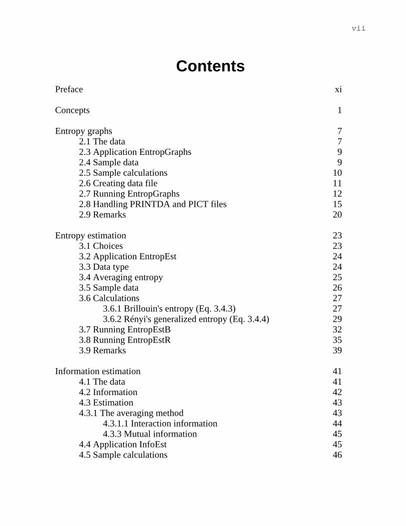
Contents

Preface xi Concepts 1 Entropy graphs 7

2.1 The data 7 2.3 Application EntropGraphs 9 2.4 Sample data 9 2.5 Sample calculations 10 2.6 Creating data file 11 2.7 Running EntropGraphs 12 2.8 Handling PRINTDA and PICT files 15 2.9 Remarks 20

Entropy estimation 23

3.1 Choices 23 3.2 Application EntropEst 24 3.3 Data type 24 3.4 Averaging entropy 25 3.5 Sample data 26 3.6 Calculations 27

3.6.1 Brillouin's entropy (Eq. 3.4.3) 27 3.6.2 Rényi's generalized entropy (Eq. 3.4.4) 29

3.7 Running EntropEstB 32 3.8 Running EntropEstR 35 3.9 Remarks 39

Information estimation 41

4.1 The data 41 4.2 Information 42 4.3 Estimation 43 4.3.1 The averaging method 43

4.3.1.1 Interaction information 44 4.3.3 Mutual information 45

4.4 Application InfoEst 45 4.5 Sample calculations 46

viii ECOLOGICAL COMPUTATIONS SERIES: VOL. 3

viii

4.5.1 Interaction information 46 4.5.2 Mutual information 51

4.6 More data 54 4.7 Running InfoEst 57 4.8 Remarks 65

Glossary 67 Bibliography 69

ix

ix

Preface Information theoretical tools are described which help the user to quantify

such structural properties as diversity, mutuality1 and equivocation. Rényi's

generalized entropy and information are the basic physical quantities. Unlike the

familiar Shannon, Brillouin, Kullback measures (SBK), Rényi's entropy and

information have "order". This is a potent and desired quality when a goal is to

achieve structural descriptions of generality and flexibility.

The conventional SBK measures supply point descriptions of community

and population structure. These contrast with the Rényi measures which allow

viewing community and population structures under conditions of changing order.

Changing order generates a scale process in which magnification and sharpness

interplay to discriminate between cases. But the choice of order is arbitrary and

1 Interaction, association.

x ECOLOGICAL COMPUTATIONS SERIES: VOL. 3

x

some may not be prepared to make this choice. Instead, they may opt for vector

descriptions or curves as shown in the 2nd chapter. On these curves the SBK

quantities are points. The Shannon entropy, for instance, as a 1st order measure is a

point in the vicinity of an infinitesimal break on the curve. On one side lies the

Simpson point, a 2nd order entropy. The log state (species) richness index, the 0

order entropy measure, is an extreme point on the opposite side. It is well to

remember that the structural magnification at these lower order entropy measures is

rather poor, being worst at order zero. It should also be noted that any point on the

entropy curve at orders greater than one can serve as a diversity measure with more

discriminating power than the Shannon or Brillouin index. In a similar vain, the

idea that association or interaction can have different orders will render the

Kullback statistic (MDIS) or the Pearson's χ2, which are 1st order measures, not so

attractive for the ecologist.

The successive sections will clarify these propositions and also offer

guidance to programs in CANAPACK which compute entropy graphs, entropy

estimates and information estimates under process sampling2. The programs are

conversational and completely self-contained. They run on any Macintosh in good

order with a reasonably large RAM and disk memory. The minimum required

RAM size will depend on the size of the code and on the size of the arrays. Code

sizes are obtainable for individual applications from the disk directory. The arrays

depend on the data to be analyzed. Since the arrays are dynamically defined, the

2 Orlóci and De Patta Pillar 1989. -- The proposition in process sampling is reminiscent of Poore's (1955,1956) successive approximation approach and the flexible analysis of Wildi and Orló ci (1987). The term "process" conjures a view of sampling in which step-by-step expansions are intricately tide to a monitoring of the evolution of the sample structures and structural connections in concurrent data analysis, based on which stability is judged. When structural stability is detected the sampling stops. Juhász-Nagy and Podani (1983), Podani (1984), Orlóci (1988), Kenkel, Juhász-Nagy and Podani (1989) and other works, to which they refer, are relevant references.

PREFACE xi

xi xi

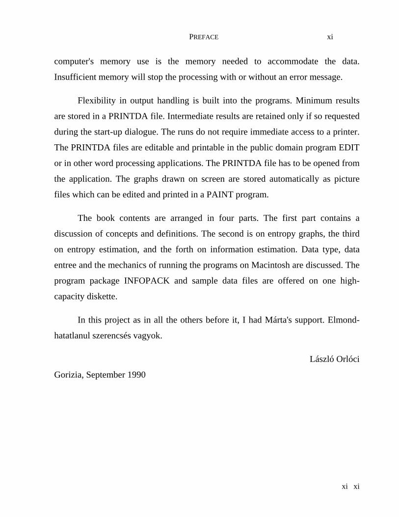
computer's memory use is the memory needed to accommodate the data.

Insufficient memory will stop the processing with or without an error message.

Flexibility in output handling is built into the programs. Minimum results

are stored in a PRINTDA file. Intermediate results are retained only if so requested

during the start-up dialogue. The runs do not require immediate access to a printer.

The PRINTDA files are editable and printable in the public domain program EDIT

or in other word processing applications. The PRINTDA file has to be opened from

the application. The graphs drawn on screen are stored automatically as picture

files which can be edited and printed in a PAINT program.

The book contents are arranged in four parts. The first part contains a

discussion of concepts and definitions. The second is on entropy graphs, the third

on entropy estimation, and the forth on information estimation. Data type, data

entree and the mechanics of running the programs on Macintosh are discussed. The

program package INFOPACK and sample data files are offered on one high-

capacity diskette.

In this project as in all the others before it, I had Márta's support. Elmond-

hatatlanul szerencsés vagyok.

László Orlóci

Gorizia, September 1990

xii ECOLOGICAL COMPUTATIONS SERIES: VOL. 3

xii

1

1 Concepts The idea that entropy expresses disorder is central in science. Interestingly

one of the most fundamental physical laws, Boltzman's 2nd law of

thermodynamics, is about entropy and disorder. The relationship is such that

entropy is low in orderly systems and high in disorderly systems. In translation,

increasing entropy is the ally of stability, the omega state in the direction of which

natural systems are pointed as they march through their evolution. By the same

token, increasing entropy is also the ally of unpredictability in which lies the

paradox that predictability is not a trait of natural stability.

In the most general case the tendency of increased entropy is a property of

an expanding universe3. With this said but not explained, entropy is regarded a key

3 Increasing entropy gives time its "arrow", says A. Eddington, and makes us remember the past but not to know the future, remarks S. W. Hawking.

2 ECOLOGICAL COMPUTATIONS SERIES: VOL. 3

physical attribute of the bioenvironmental system. Through the measurement of

entropy, some believes4 the very essence of the bioenvironmental process can be

captured.

It is customary to measure entropy as a logarithm of proportions,

H = - K ∑=

n

i ii p log p

1 Eq. 1.1

This is Shannon's fundamental equation for the description of the symbol structure

in signals that carry the message from source to destination. Anything that can

distort the symbol structure and cause a discrepancy between the messages sent (x)

and the message received (y) is called "noise"5. This discrepancy is a source of

uncertainty at the time of interpretations. To measure it, Shannon uses

Hx(y) = - K )(jp log pn

jiij∑

=1 Eq. 1.2

which he termed equivocation information6. Others refer to Hx(y) as specific

entropy unique to x in comparison to entropy in y. Hx(y) is high when the structural

distortion in the received message is high. Obviously Hx(y) need not be the same as

Hy(x.)

4 R. Margalef asserts that as the system evolves, entropy "grows" about itself. 5 This is irrespective of the substance of the message.

6 pi(j) is the conditional probability of symbol j in y for given symbol i in x, defined by

pi(j) = pijpi

= i

ij

ff

In this fij is the joint frequency of the ith and jth symbols.

CONCEPTS 3

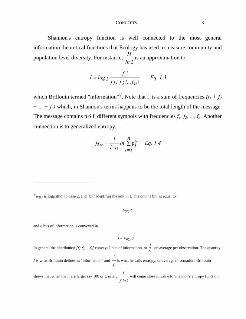
Shannon's entropy function is well connected to the most general

information theoretical functions that Ecology has used to measure community and

population level diversity. For instance, 2ln

H is an approximation to

!nf!...2f!1f!.flog2I = Eq. 1.3

which Brillouin termed "information"7. Note that f. is a sum of frequencies (f1 + f2

+ ... + fn) which, in Shannon's terms happens to be the total length of the message.

The message contains n δ f. different symbols with frequencies f1, f2, ..., fn. Another

connection is to generalized entropy,

∑=−

=n

1iailn

11

H pαα Eq. 1.4

7 log2 is logarithm to base 2, and "bit" identifies the unit in I. The unit "1 bit" is equal to

log2 2

and n bits of information is conveyed in

I = log2 2n .

In general the distribution [f1 f2 ... fs] conveys I bits of information, or If. on average per observation. The quantity

I is what Brillouin defines as "information" and .f

Iis what he calls entropy, or average information. Brillouin

shows that when the fi are large, say 100 or greater, 2ln.f

Iwill come close in value to Shannon's entropy function.


which Rényi derived as "entropy of order α". In Rényi's terms, Shannon's entropy

is 1st order entropy8.

The term "information" means different things to different authors. What

Brillouin describes as information (Eq. 1.3) is a multiple of the quantity that others

describe as entropy in a single distribution. Brillouin's information is not the same

as Rényi's which is a divergence measure on two distributions

P = (p1 p2 ... pn) and Q = (q1 q2 ... qn )

and which has order (α):

1ai

ain

1i p

qln

11

I −=∑

−=

αα Eq.1.5

When α approaches 1, i is information in Kullback's terms

i

ii

n

1i p

qlnqf.2I =2 ∑

= Eq.1.6

The elements in P and Q are uniquely paired so that every qi has a corresponding

pi. No restrictions need be applied regarding the distribution totals or the level of

summation in Eq.1.5, excepting the Kullback's manipulations in which case the

two distributions must have equal totals and the summations must run through all n

terms. The latter is desired when analytical and probabilistic connection are sought

between "information" and Pearson's chi-squared.

8 Eq. 1 is not defined for α = 1. The derivation is not simple and for details the l'Hospital's rule of calculus should be revisited.

CONCEPTS 5

The applications of information theoretical notions in Biology have derived

their conceptual basis and also to some extent their methodology from the classics:

C. E. Shannon, L. Brillouin, S. Kullback, A. Rényi9. It is clear that information

theory offers the advantage of universal identifiability when describing population

and community structures and structural connections. The specific methodologies

that are centered around the cases of Eq.1.1 and Eq.1.6 include systems modelling,

diversity estimation, and statistical data analysis:

ENTROPY BASED BIOLOGICAL MODELLING. Very much in fashion in the 1950's,

the early efforts ended in disillusionments -- according to the story narrated in

Yockey, Platzman and Quastler (1958.) The early models apparently produced no

new biological insight. This should of course not reflect negatively on information

theory, but rather it should point up the inadequacy of knowledge at that time about

the systems that they tried to model.

DIVERSITY ESTIMATION. The idea of uncertainty being at its maximum when

entropy is at its highest, has made the entropy concept a foundation of diversity

theory. In fact reasoning from entropy appears early in work on community

structure10, but the applications that followed were straight jacketed by the authors

not recognizing that diversity can have different orders. In this respect the full

impact of A. Rényi's mathematical work has yet to materialize in diversity

studies11.

STATISTICAL DATA ANALYSIS. The analysis of community and population level

relationships is among the more developed fields in the biological applications of 9 See the Bibliography for key references. 10 See R. Margalef's and E. C. Pielou's seminal works on the topic (1958, 1975). 11 O. H. Hill's (1973) work which my comments on his early manuscript triggered is exceptional, but has apparently not been followed.


information theory, but these too are largely limited to 1st order information

divergence measures12 which largely owe their familiarity to S. Kullback's seminal

work on an information based statistical methodology. A. Rényi's umbrella theory

should spear further developments in these and other realms of data analysis not

yet charted by applied work.

12 Kullback (1959, 1968) and also Rényi (1961), Rajski (1961).

7

2 Entropy graphs The frequency distribution of a single variable is the basic data source and

Eq. 1.4 is the entropy function. The entropy graph is the graph of this function

generated by the process of changing the value of α. Any value 0 and up is

permitted except exactly 1.

2.1 The data

The states of a discrete variable X are involved. The jth state has frequency fj. There are s states and the frequency distribution is

F = (f1 f2 ... fs)


The distribution total is f.13. The states may or may not have a unique order.

2.2 Descriptors of F and limits

The descriptors include the number of cells s and a graph of Rényi's entropy

as a function of α. F has two limiting distributions,

F l = (f. - s + 1 1 ... 1) Eq. 2.2

the least dispersed, and

F m = ( f

_ f

_ ... f

_ ) Eq. 2.3

the most dispersed. In the latter f_

= . F l and F

m are both s-valued and f.-totalled.

The entropy in F l is defined by

−+

−=

f .α)(s

f .αs)(f .α

-α aH 11ln11 Eq. 2.4

This is the possible lowest entropy in an s-valued distribution with f. total and

given α. The entropy in Fm,

H α = ln s Eq. 2.5

is the possible highest entropy in an s-valued frequency distribution regardless of f.

or α.

13 A dot in the subscript indicates summation over the subscript replaced by the dot. For example, f1. = f11 + f12 + ... + f1k.

ENTROPY GRAPHS 9

2.3 Application EntropGraphs This program computes entropy quantities of different order based frequency

or density data. Any number of distributions are permitted and in each case H α

graphs are drawn for F m , F, F

l in that order. The α axis is scaled from 0 to a

specified upper α value in 1/1000 parts. Tick marks are places as requested. The

drawing automatically adjusts to screen size on tested equipment.

2.4 Sample data

Raunkiaer's biological spectra of different locations given in Braun-

Branquet14 are analyzed:

Spectrum name Life-form F Ch H G Th _____________________________________________ Normal 46 9 26 6 13 Spitzbergen 1 22 60 15 2 Death Valley 26 7 18 7 42 Seychelles 61 6 12 5 16 Connecticut 15 2 49 22 12 Paris basin 8 6 52 25 9

Life-forms are the survival types of plant individuals, such as phanerophyte (F),

chamaephyte (Ch), hemicryptophyte (H), geophyte (G), and therophyte (Th). This

system is particularly well suited for use in character based community studies.

2.5 Sample calculations

In the Raunkiaer data set s is uniformly 5 and f. is uniformly 100. Such a

uniformity is not required as a rule. The maximum entropy (Eq. 2.5) is uniformly 14 1932, p. 298.


Ho = ln 5 = 1.60944 or 2.32193 bits

regardless of α. The minimum entropy (Eq. 2.4) is also the same for each of the

spectra, but this depends on α.

Consider the normal spectrum

F = (46 9 26 6 13)

and the case of α = 0.7. For this,

f. = 100

H0.7 = 7.01

)13.006.026.009.046.0ln( 7.07.07.07.07.0

−++++

= 1.42796

max H0.7 = 1.60944

min H0.7 = ln (0.960.7 + 4 x 0.010.7)

1 - 0.7 = 0.41055 .

Similar computations emit other Hα values for any α except α = 1 in which case

Eq. 1.1 is appropriate:

H1 = 0.46 ln 0.46 + 0.09 ln 0.09 + 0.26 ln 0.26 +

+ 0.06 ln 0.06 + 0.13 ln 0.13 = 1.35819

min H1 = -(0.96 ln 0.96 + 0.04 ln 0.01) = 0.22340

2.6 Creating data file

ENTROPY GRAPHS 11

Data are presented for analysis in an ASCII text file on disk. For the

Raunkiaer spectra, this file is 30-valued:

46 9 26 6 13 1 22 60 15 2 26 7 18 7 42 61 6 12 5 16 15 2 49 22 12 8 6 52 25 9

Note that the data file does not contain zeros (as a rule) and there are no blank lines

in the file (also a rule.) The data file begins with a number (no leading blank lines),

data entree is by distribution, and each number entered is followed by an END-OF-


PARAGRAPH mark, except the last number where this is optional. The END-OF-

PARAGRAPH mark is created by pressing the RETURN key after typing the

number.

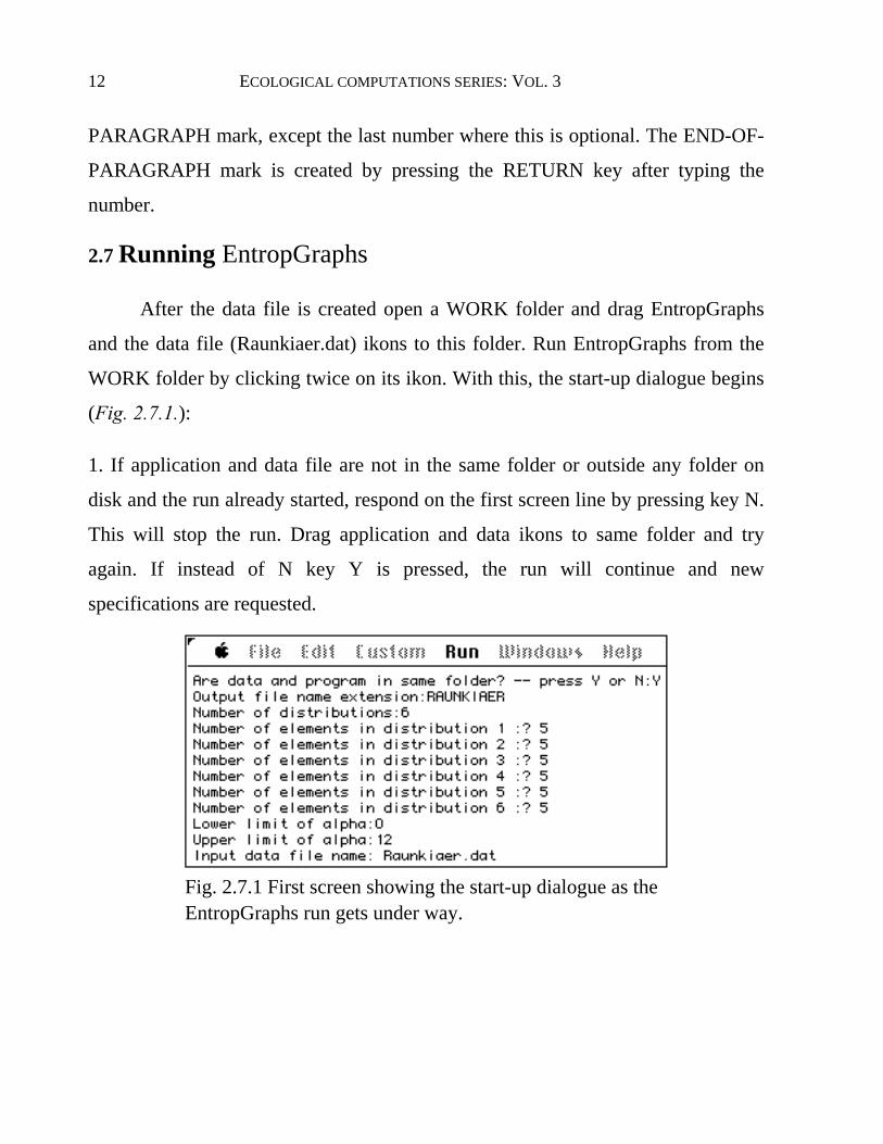
2.7 Running EntropGraphs

After the data file is created open a WORK folder and drag EntropGraphs

and the data file (Raunkiaer.dat) ikons to this folder. Run EntropGraphs from the

WORK folder by clicking twice on its ikon. With this, the start-up dialogue begins

(Fig. 2.7.1.):

1. If application and data file are not in the same folder or outside any folder on

disk and the run already started, respond on the first screen line by pressing key N.

This will stop the run. Drag application and data ikons to same folder and try

again. If instead of N key Y is pressed, the run will continue and new

specifications are requested.

Fig. 2.7.1 First screen showing the start-up dialogue as the EntropGraphs run gets under way.

ENTROPY GRAPHS 13

2. The output file name extension identifies the PRINTDA file where the PRINT

output and run information are stored, and the PICT file(s) in which the entropy

graphs are stored. For example, if RANUNKIAER (lower or uppercase) is typed as

the output file name extension, the print file will have full name

PRINTDA.RAUNKIAER and the PICT files will have full names

PICT.RAUNKIAER/1, PICT.RAUNKIAER/2, etc. There will be as many PICT

files created in the run as there are distributions specified on screen line 3.

3. The number of elements (screen lines 4 to 9) may differ depending on the

distribution.

If fewer numbers are found in the data file than the number

specified in the dialogue, or if blank lines are present, the

program will stop. Thorough checking is in order before the

next attempt to run EntropGraphs.

4. The lower limit of α may be 0 or a value higher than zero, but not exactly 1. The

upper limit should be any positive number, except exactly 1.

5. The data file name is the full name in the disk directory, such as Raunkiaer.dat.

Do not press the RETURN key after input when an option is specified.

EntropGraphs assumes GET KEY input in such a case.


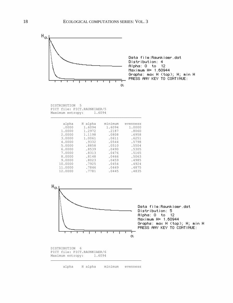
Fig. 2.7.2 An intermediate scree in the run of EntropGraphs. Information and graphs are shown for the Spitzbergen spectrum (Section 2.4.) The values of H

α are on the vertical axis. The α values are plotted on the horizontal axis from 0 to 12 in steps of 1.

After completion of the opening dialogue the progressive screens will

display graphs and graph information. Fig. 2.7.2 is an example. The program

pauses after drawing the graph and the message PRESS ANY KEY TO

CONTINUE appears on the screen. This halts the processing to give the user time

to inspect the screen. Processing resumes when a key is pressed. The graph is

automatically stored (PICT.RAUNKIAER/1, etc.) The final screen is shown in Fig.

2.7.3.

ENTROPY GRAPHS 15

Fig. 2.7.3 Last screen in the run of application EntropGraphs.

2.8 Handling PRINTDA and PICT files

The run information and the results are accessed by opening the PRINTDA

file from application EDIT. The contents of PRINTDA.RAUNKIAER are

displayed in Table 2.8.1. The graphs and graph information from the PICT files are

inserted in the same table. Since EDIT is not suitable for the latter operation, a

paint program is needed to open the picture files for editing and a word processing

program is needed which can accept files from the paint program.

Table 2.8.1 Contents of file PRINTDA.RAUNKIAER with graphs inserted from the PICT.RAUNKIAER files.

PROGRAM EntropGraphs _____________________________________________________ Entropy of order alpha is computed and entropy graphs

drawn for F and the limiting F m and F

l.

Lower limit alpha = 0 Upper limit alpha = 12 Input data file name: Raunkiaer.dat DISTRIBUTION 1 PICT file: PICT.RAUNKIAER/1 Maximum entropy: 1.6094 ____________________________________________ alpha H alpha minimum evenness .0000 1.6094 1.6094 1.0000 1.0000 1.3555 .2187 .8422 2.0000 1.1766 .0808 .7311 3.0000 1.0673 .0611 .6631 4.0000 .9999 .0544 .6213 5.0000 .9557 .0510 .5938 6.0000 .9250 .0490 .5747 7.0000 .9026 .0476 .5608 8.0000 .8858 .0466 .5504 9.0000 .8727 .0459 .5423 10.0000 .8623 .0454 .5358


11.0000 .8539 .0449 .5306 12.0000 .8469 .0445 .5262

DISTRIBUTION 2 PICT file: PICT.RAUNKIAER/2 Maximum entropy: 1.6094 ____________________________________________ alpha H alpha minimum evenness .0000 1.6094 1.6094 1.0000 1.0000 1.0448 .2187 .6492 2.0000 .8390 .0808 .5213 3.0000 .7338 .0611 .4560 4.0000 .6733 .0544 .4183 5.0000 .6363 .0510 .3953 6.0000 .6122 .0490 .3804 7.0000 .5956 .0476 .3701 8.0000 .5836 .0466 .3626 9.0000 .5746 .0459 .3570 10.0000 .5675 .0454 .3526 11.0000 .5618 .0449 .3491 12.0000 .5572 .0445 .3462

DISTRIBUTION 3 PICT file: PICT.RAUNKIAER/3 Maximum entropy: 1.6094 ____________________________________________ alpha H alpha minimum evenness .0000 1.6094 1.6094 1.0000

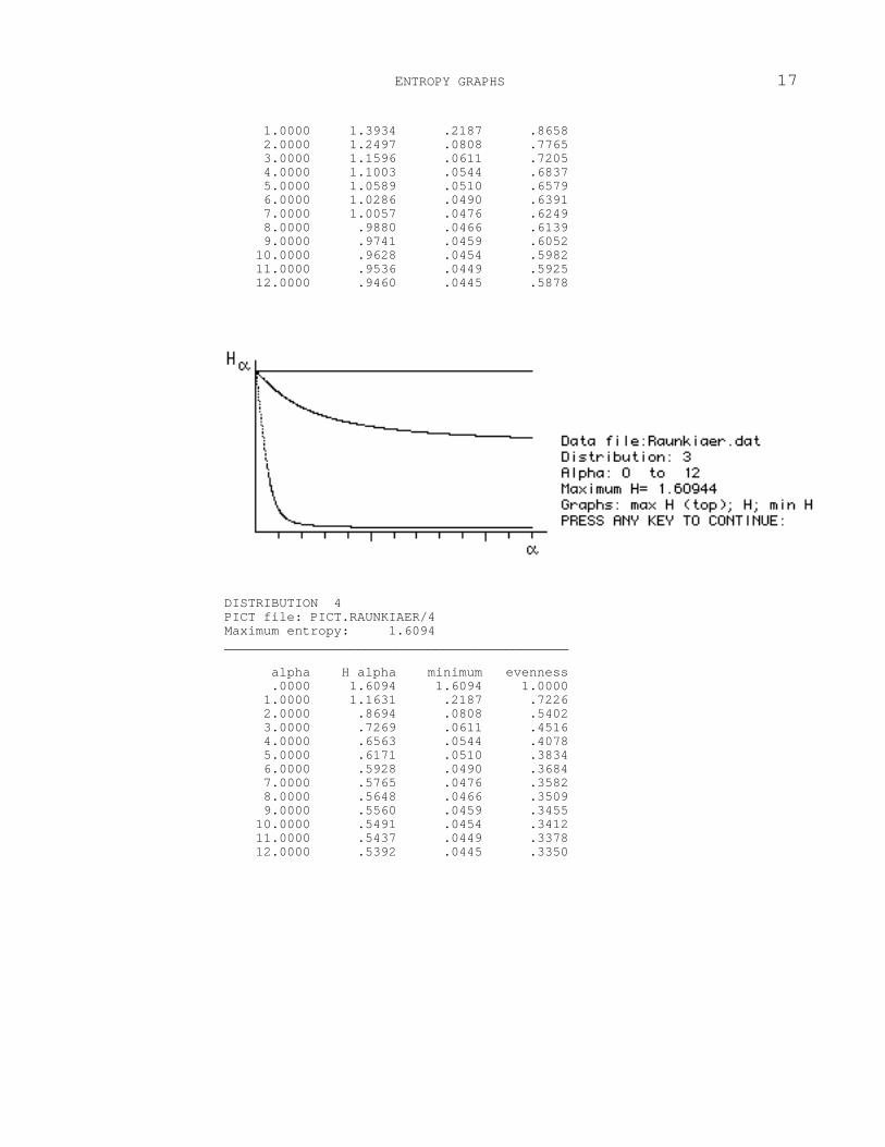
ENTROPY GRAPHS 17

1.0000 1.3934 .2187 .8658 2.0000 1.2497 .0808 .7765 3.0000 1.1596 .0611 .7205 4.0000 1.1003 .0544 .6837 5.0000 1.0589 .0510 .6579 6.0000 1.0286 .0490 .6391 7.0000 1.0057 .0476 .6249 8.0000 .9880 .0466 .6139 9.0000 .9741 .0459 .6052 10.0000 .9628 .0454 .5982 11.0000 .9536 .0449 .5925 12.0000 .9460 .0445 .5878

DISTRIBUTION 4 PICT file: PICT.RAUNKIAER/4 Maximum entropy: 1.6094 ____________________________________________ alpha H alpha minimum evenness .0000 1.6094 1.6094 1.0000 1.0000 1.1631 .2187 .7226 2.0000 .8694 .0808 .5402 3.0000 .7269 .0611 .4516 4.0000 .6563 .0544 .4078 5.0000 .6171 .0510 .3834 6.0000 .5928 .0490 .3684 7.0000 .5765 .0476 .3582 8.0000 .5648 .0466 .3509 9.0000 .5560 .0459 .3455 10.0000 .5491 .0454 .3412 11.0000 .5437 .0449 .3378 12.0000 .5392 .0445 .3350


DISTRIBUTION 5 PICT file: PICT.RAUNKIAER/5 Maximum entropy: 1.6094 ____________________________________________ alpha H alpha minimum evenness .0000 1.6094 1.6094 1.0000 1.0000 1.2972 .2187 .8060 2.0000 1.1198 .0808 .6958 3.0000 1.0061 .0611 .6251 4.0000 .9332 .0544 .5798 5.0000 .8858 .0510 .5504 6.0000 .8539 .0490 .5305 7.0000 .8313 .0476 .5165 8.0000 .8148 .0466 .5063 9.0000 .8023 .0459 .4985 10.0000 .7925 .0454 .4924 11.0000 .7846 .0449 .4875 12.0000 .7781 .0445 .4835

DISTRIBUTION 6 PICT file: PICT.RAUNKIAER/6 Maximum entropy: 1.6094 ____________________________________________ alpha H alpha minimum evenness

ENTROPY GRAPHS 19

.0000 1.6094 1.6094 1.0000 1.0000 1.2707 .2187 .7895 2.0000 1.0450 .0808 .6493 3.0000 .9225 .0611 .5732 4.0000 .8534 .0544 .5302 5.0000 .8106 .0510 .5036 6.0000 .7820 .0490 .4859 7.0000 .7617 .0476 .4733 8.0000 .7468 .0466 .4640 9.0000 .7354 .0459 .4569 10.0000 .7264 .0454 .4513 11.0000 .7192 .0449 .4469 12.0000 .7133 .0445 .4432

2.9 Remarks

Each graph contains a straight horizontal line on top and two curves. These

represent the entropy in distributions F m , F and Fl. The following are useful to

remember when attempting to interpret the results:

1. Entropy is a physical property. When entropy is maximal, the disorder is

maximal, the predictability of specific states is minimal and diversity is maximal

(case F m .) Conversely, when entropy is lowest, diversity is minimal (case F

1 .)

Entropy and therefore diversity has order.

2. Entropy of any order is expressible in "evenness" terms,

s

aHE ln

=α


This depicts the relative closeness of F to Fm. Eα should not be confused with Iα

(Eq. 1.5) which expresses the divergence of F from Fm.

3. Entropy of orders 0, 1 and 2 denotes cases that biologists have used as diversity

indices:

H 0 = ln s -- state (species) richness index.

H = - ∑j=1

s pj ln pj -- Shannon index.

H 2 = - ln ∑

j=1

S p2

j -- log Simpson index.

The state richness index is the maximum value that the other two indices can

possibly attain. The Shannon index is far the most popular, albeit a rather odd point

on the entropy graph where the measured value may undergo a dramatic rise, or

fall with even a relatively small change in α. It would be better to use another point

on the entropy graph at an α where the curve begins leveling off. Alternatively, the

entire graph extending from α = 0 up to some chosen α value may be used.

4. Entropy comparisons may involve the H α values directly between distributions

of equal s. In other cases where s is not constant, the minimum value, maximum

value and the evenness index should also be considered jointly.

5. Regarding Raunkiaer's biological spectra (Section 2.4) the contents of Table

2.9.1 are relevant. Note that in the spectra s = 5 uniformly which makes the

maximum entropy uniformly ln 5. The minimum entropy does not under go

change, since the s value is constant and the spectral totals are constant. Note the

use of entropy of order 12 in the table. High order entropy amplifies the

ENTROPY GRAPHS 21

differences between the spectra. The ordering of the spectra by entropy is rather

revealing. The vegetation of a hot semi-desert has the most diverse biological

spectrum and diversity declines towards the extremes, such as the wet tropics and

the tundra. Considering that the Raunkiaer spectrum reflects the survival

characteristics of individual plants, it may even be argued that the vegetation in the

hot semi-desert have greater stability than in the wet tropics or the tundra.

Table 2.9.1 The Raunkiaer spectra (Section 1.2) ordered according to high-order entropy.

Spectrum Entropy Evenness

max H H12 min H12 _____________________________________________________________________________________________

Death Valley 1.6094 .9460 .0445 .5878 Normal spectrum .8469 .5262 Connecticut .7781 .4835 Paris basin .7133 .4432 Spitzbergen .5572 .3462 Seychelles .5392 .3350

22

3 Entropy estimation The data source is process sampling through k surges and the estimated

quantity is Brillouin's entropy (Eq. 1.3) Rényi's entropy of order α (Eq. 1.4.) The

averaging technique is Pielou's15.

3.1 Choices

E. C. Pielou argues the question of choice and comes down in favour of the

Brillouin equation. She is concerned with the potential of the Shannon entropy

function (Eq. 1.1) being inaccurate in small populations. It is interesting, however,

to note that her concern is not generally shared. In fact others, most notably C. E.

Shannon, A. Rényi and S. Kullback approach information theory based on Eq. 1.1,

15 1975.

ENTROPY ESTIMATION 23

Eqs. 1.4, 1.5 and Eq. 1.6, not Eq. 1.3. In all of these cases the Brillouin information

is not considered a benchmark value.

3.2 Application EntropEst

Program EntropEst has two versions, EntropEstB and EntropEstR.

EntropEstB computes Brillouin's function based on the natural logarithm.

EntropEstR computes Rényi's entropy of order α for legitimate values of α from

zero up to a chosen limit in increments of 1.

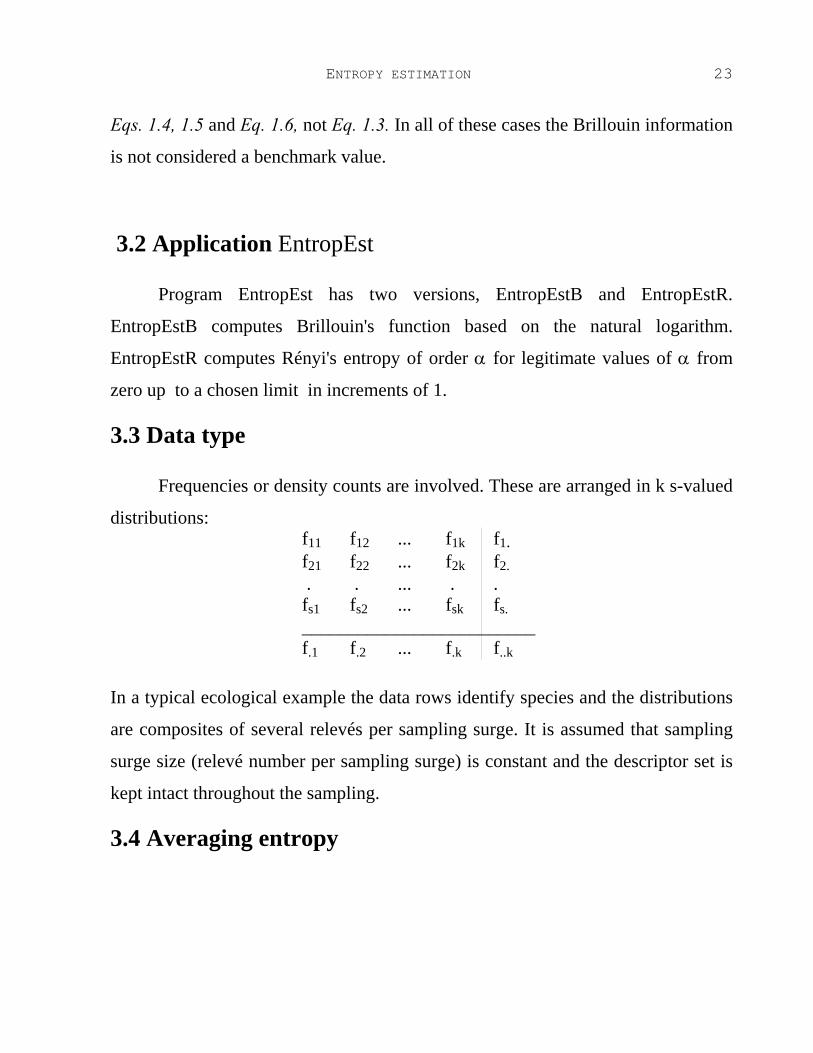
3.3 Data type

Frequencies or density counts are involved. These are arranged in k s-valued

distributions: f11 f12 ... f1k f1. f21 f22 ... f2k f2. . . ... . . fs1 fs2 ... fsk fs. _________________________ f.1 f.2 ... f.k f..k

In a typical ecological example the data rows identify species and the distributions

are composites of several relevés per sampling surge. It is assumed that sampling

surge size (relevé number per sampling surge) is constant and the descriptor set is

kept intact throughout the sampling.

3.4 Averaging entropy


After each sampling surge an entropy value is computed for each α and

averaged with the previous entropy values. One may be tempted to use the

weighted average in u = k sampling surges,

ufauHufaHfaHf

H u..

....22.11. ';

+++=θα

which is equivalent to

∑=

∑=−

=s

iaijp

u

jf j..ua)f(Hα;θu 1

ln11

1 Eq. 3.4.1

where

jfijf

pij.

But H'α; ∅u is not optimal, since it does not incorporate terms for shared

information which links the u sampling surges into an entropy process. The

following expression does include a term for shared information:

H*α; ∅u = H'

α; ∅u + Hα; →u(descriptors;sampling)

Considering entropy of order 1,

H*1; ∅u = -

1f..u

∑

j=1

u ∑i=1

s fij ln

fijf.j + ∑

j=1

u ∑i=1

s fij ln

fijf..ufi.uf.j

= - 1f..u ∑

i=1

s fi.u ln

fi.uf..u Eq. 3.4.2

which happens to be a multiple of Shannon's entropy. The corresponding Brillouin

entropy is


H*∅u =

1f..u ln

f..u!f1.u! f2.u! ... fs.u! . Eq. 3.4.3

and the generalized entropy is

H*α∅u =

11 - α ln ∑

i=1

s p

αi.u Eq. 3.4.4

with proportions defined according to

p i.u =

f i.uf ..u

****3.5 Sample data

Consider density estimates for 3 species in quadrat samples of constant

sampling fraction emitting from a 6-step sampling process:

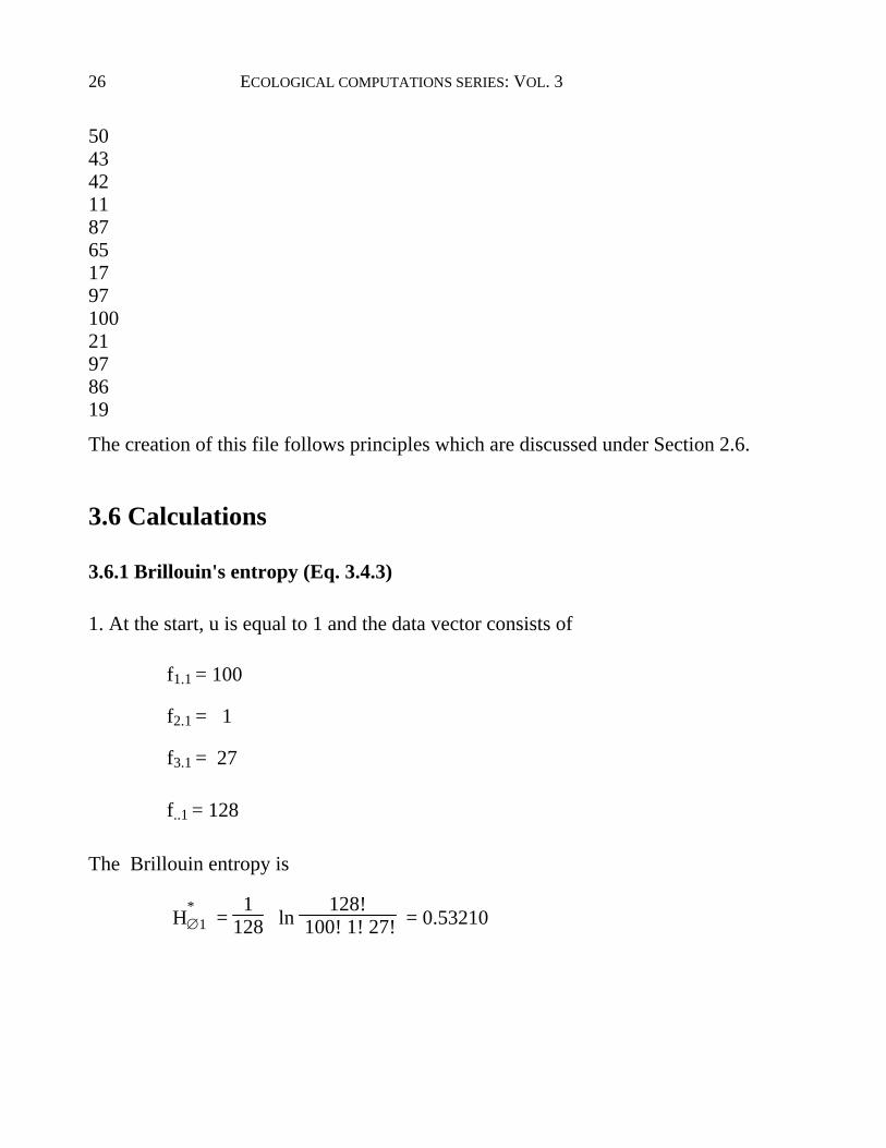
Species Distribution 1 2 3 4 5 6 ____________________________________________ 1 100 93 43 87 97 97 2 1 26 42 65 100 86 3 27 50 11 17 21 19 ____________________________________________ Total 128 169 96 169 218 202

This data set is entered on file (Density.dat) by distribution (column): 100 1 27 93 26


50 43 42 11 87 65 17 97 100 21 97 86 19

The creation of this file follows principles which are discussed under Section 2.6.

3.6 Calculations

3.6.1 Brillouin's entropy (Eq. 3.4.3)

1. At the start, u is equal to 1 and the data vector consists of

f1.1 = 100

f2.1 = 1

f3.1 = 27

f..1 = 128

The Brillouin entropy is

H*∅1 =

1128 ln

128! 100! 1! 27! = 0.53210


or 0.53210/ln 2 = 0.76766 bits16.

2. For u = 2,

f1.2 = 193

f2.2 = 27

f3.2 = 77

f..2 = 297

H*∅2 =

1297 ln

297! 193! 27! 77! = 0.82974 .

3. For other u:

H*∅3 = 0.93166

H*∅4 = 0.96229

H*∅5 = 0.98045

H*∅6 = 0.97858 .

4. If the 6 values were graphed, the graph segment from point 3 on may be taken as

being "flat" and the entropy estimates will accord with

H ∅u =

|f..u H*∅u - f..u-1 H*

∅u-1| f..u - f..u-1

; u = 1, ..., 6

Numerically,

H ∅4 =

562 x 0.96229 - 393 x 0.93166 562 - 393 = 1.03352

16 To minimize the rounding errors in long-hand computations, retain an ample number of digits in intermediate steps.


H ∅5 = 1.02726

H ∅6 = 0.97134.

The average of these is the entropy estimate sought17:

H = 1

k - IP ∑u=IP+1

k H

∅u = 1.03352 + 1.02726 + 0.97134

6 - 3 = 1.01071

An estimate of the sampling variance of H is

S2H =

1(k - IP)(k - IP - 1) ∑

u=IP+1

k (H

∅u - H)2

= (1.03352-1.01071)2+(1.02726-1.01071)2+(0.97134-1.01071)2

6

= 0.00039070

3.6.2 Rényi's generalized entropy (Eq. 3.4.4)

The steps are similar as before:

1. For u=1,

f1.1 = 100

f2.1 = 1

f3.1 = 27

f..1 = 128

17 See Pielou (1964).


H* 1; ∅1 =

100128 ln

100128 +

1128 ln

1128 +

27128 ln

27128 = 0.55903

H*2; ∅1 =

11 - 2 ln

1002

1282 +

12

1282 +

272

1282

= 0.42326 .

H*3; ∅1 =

11 - 3 ln

1003

1283 +

13

1283 +

273

1283

= 3.36056

H*4; ∅1 =

11 - 4 ln

1004

1284 +

14

1284 +

274

1284

= 0.32738

Similar computations would yield any higher order entropy.

2. For u = 2,

f1.2 = 193

f2.2 = 27

f3.2 = 77

f..2 = 297

H* 1; ∅2 =

193297 ln

193297 +

27297 ln

27297 +

77297 ln

77297 = 0.84808

H*2; ∅2 =

11 - 2 ln

1932

2972 +

272

2972 +

772

2972

= 0.69764

H*3; ∅2 =

11 - 3 ln

1933

2973 +

273

2973 +

773

2973

= 0.61449


H*4; ∅2 =

11 - 4 ln

1934

2974 +

274

2974 +

774

2974

= 0.56626

Other higher order entropy values are similarly computed.

3. In the following steps, similar computations are applied to obtain entropy values

of different order. For example, for entropy of order 3,

H*3; ∅3 = 0.72795

H*3; ∅4 = 0.78051

H*3; ∅5 = 0.83742

H*3; ∅6 = 0.84709

4. Considering the H*3∅u graph and taking IP as being 3, the entropy estimate for

each sampling surge accords with

H 3; ∅u =

|f..u H*3; ∅u - f..u-1 H*

3; ∅u-1| f..u - f..u-1

; u = 3, ..., 6

Numerically,

H 3; ∅4 =

562 x 0.78051 - 393 x 0.72795 562 - 393 = 0.90273

H 3; ∅5 = 0.98414

H 3; ∅6 = 0.88442

5. Based on the above the pooled entropy estimate of order 3 is

H 3 =

1k - IP ∑

u=IP+1

k H

3; ∅u = 0.90273 + 0.98414 + 0.88442

6 - 3 = 0.92376


and the variance of this mean is

S2

H 3 =

1(k - IP)(k - IP - 1) ∑

u=IP+1

k (H

3; ∅u - H 3)2

= (0.90273-0.923763)2+(0.98414-0.923763)2+(0.88442-0.92376)2

6

= 0.00093928

These values of the mean and the variance are specific to α = 3. For other cases of

α, similar computations would be performed.

3.7 Running EntropEstB

The data file is explained in Section 3.5. After having created the data file,

open a WORK folder and drag the ikons of EntropEstB and the data file

(Density.dat) to this folder. Start up EntropEstB by clicking twice on its ikon. As

the run gets underway, respond to requests for information on the screen:

1. If application and data ikons are not in the same folder or outside any folder on

disk and the run already started, stop the run by pressing key N (do not press the

RETURN key after N) on the 1st screen line (see dialogue in Fig. 3.7.1.) Following

this, file rearrangements can be made to meet the requirements of a new run. If the

application and data ikons are in the same folder or are outside any folder on disk,

press key Y (do not press the RETURN key after Y.) The run will continue and

new specifications will be requested.


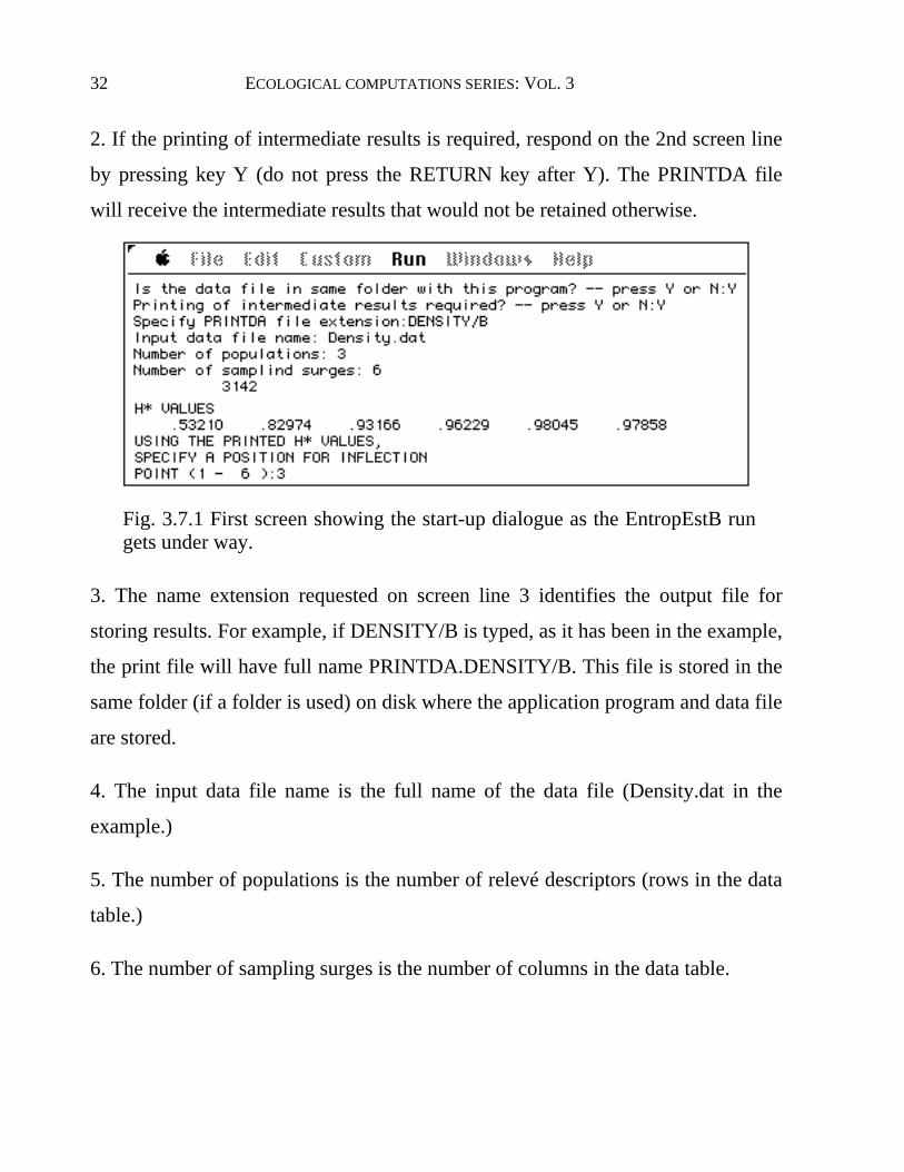
2. If the printing of intermediate results is required, respond on the 2nd screen line

by pressing key Y (do not press the RETURN key after Y). The PRINTDA file

will receive the intermediate results that would not be retained otherwise.

Fig. 3.7.1 First screen showing the start-up dialogue as the EntropEstB run gets under way.

3. The name extension requested on screen line 3 identifies the output file for

storing results. For example, if DENSITY/B is typed, as it has been in the example,

the print file will have full name PRINTDA.DENSITY/B. This file is stored in the

same folder (if a folder is used) on disk where the application program and data file

are stored.

4. The input data file name is the full name of the data file (Density.dat in the

example.)

5. The number of populations is the number of relevé descriptors (rows in the data

table.)

6. The number of sampling surges is the number of columns in the data table.


If fewer numbers are found on file then specified in the

dialogue, or if blank lines are present, the application will stop.

7. The running number seen on the 7th screen line is a count which changes as the

program computes factorials. This is just a reminder that the program is running.

8. The H*∅u values (as many in number as there are successive sampling surges)

are printed on the screen and the user is requested to pick a position which he

deems to be the "main" inflection point.

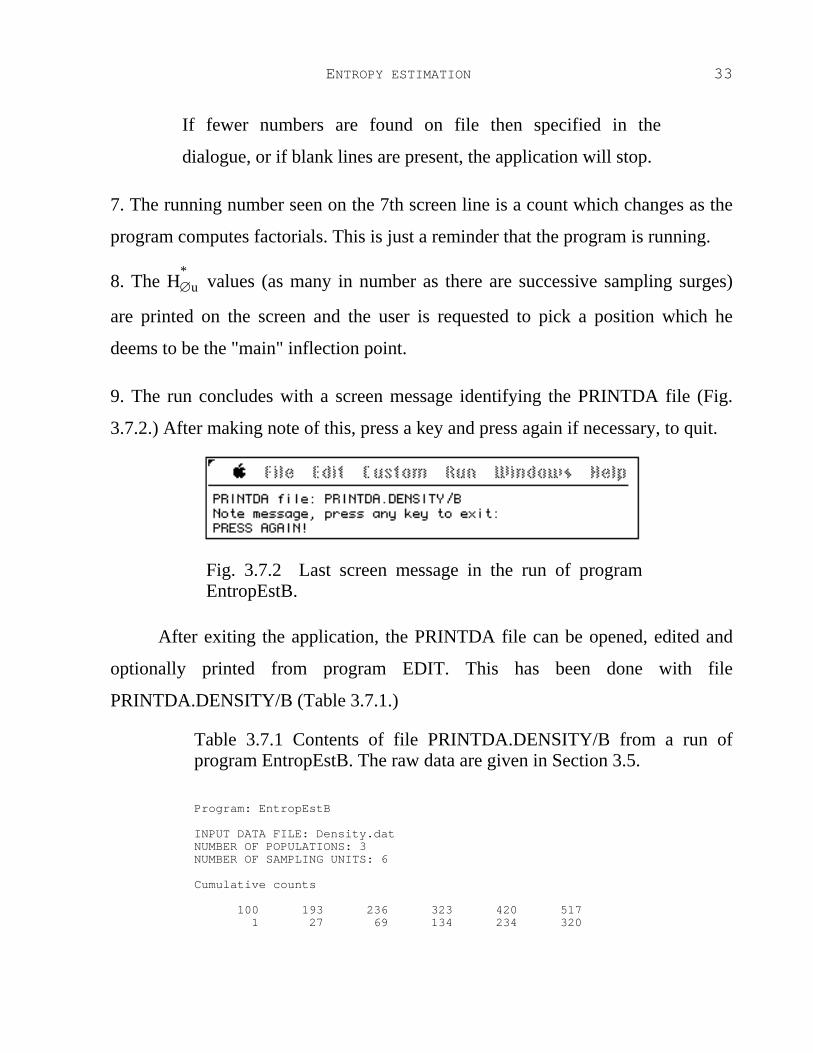
9. The run concludes with a screen message identifying the PRINTDA file (Fig.

3.7.2.) After making note of this, press a key and press again if necessary, to quit.

Fig. 3.7.2 Last screen message in the run of program EntropEstB.

After exiting the application, the PRINTDA file can be opened, edited and

optionally printed from program EDIT. This has been done with file

PRINTDA.DENSITY/B (Table 3.7.1.)

Table 3.7.1 Contents of file PRINTDA.DENSITY/B from a run of program EntropEstB. The raw data are given in Section 3.5.

Program: EntropEstB INPUT DATA FILE: Density.dat NUMBER OF POPULATIONS: 3 NUMBER OF SAMPLING UNITS: 6 Cumulative counts 100 193 236 323 420 517 1 27 69 134 234 320


27 77 88 105 126 145 Cumulative sample totals 128 297 393 562 780 982 H* values .53210 .82974 .93166 .96229 .98045 .97858 Inflection point chosen: 3 H estimates (on right side of inflection point) 1.03352 1.02726 .97134 Mean H = 1.010706 Maximum H = 1.098612 Variance of H = .00117210 Variance of the mean H = .00039070

3.8 Running EntropEstR

The start-up dialogue (Fig. 3.8.1) is similar to that discussed in Section 3.7.

There is a difference though on the 7th screen line which requests the user to

specify the upper limit of α. The starting value is zero and the step size is 1. At

each step, the program computes the H*α; ∅u values, as many in number as there are

columns in the data table (Section 3.5). These values are printed on the screen and

the user is asked to pick a position to serve as the main inflection point.


Fig. 3.8.1 First screen displaying the start-up dialogue in a run of program EntropEstR.

To exit the run press a key and repeat as needed after the last screen message (Fig.

3.8.2). The contents of the file PRINTDA.DENSITY/R are displayed in Table

3.8.1.


Fig. 3.8.2 Last screen in the run of application EntropEstR.

Table 3.8.1 The contents of PRINTDA.DENSITY/R written in the sample run of program EntropEstR

PROGRAM EntropEstR Data file:Density.dat Number of populations: 3 Number of sampling surges: 6 CUMULATIVE COUNTS 100 193 236 323 420 517 1 27 69 134 234 320 27 77 88 105 126 145 CUMULATIVE COLUMN TOTALS 128 297 393 562 780 982 H-ASTERISC VALUES AT ALPHA= 0 1.09861 1.09861 1.09861 1.09861 1.09861 1.09861 Hu of order 0 in position 1 AND UP: 1.09861 1.09861 1.09861 1.09861 1.09861 1.09861 H-ASTERISC VALUES AT ALPHA= 1 .55903 .84808 .94678 .97357 .98901 .98559 Hu of order 1 in position 3 AND UP: .55903 .84808 .94678 1.03587 1.02881 .97240 H-ASTERISC VALUES AT ALPHA= 2 .42326 .69764 .81740 .86257 .90131 .90345


Hu of order 2 in position 3 AND UP: .42326 .69764 .81740 .96760 1.00119 .91170 H-ASTERISC VALUES AT ALPHA= 3 .36054 .61449 .72795 .78051 .83742 .84709 Hu of order 3 in position 3 AND UP: .36054 .61449 .72795 .90273 .98414 .88442 H-ASTERISC VALUES AT ALPHA= 4 .32738 .56626 .67121 .72514 .79227 .80795 Hu of order 4 in position 3 AND UP: .32738 .56626 .67121 .85056 .96533 .86852 Alpha = 0 Inflection point selected: 1 Mean H = 1.09861 Variance of estimate H = -2.22045e-16 Sampling variance =-4.44089e-17 Maximum H: 1.09861 Evenness: 1 Alpha = 1 Inflection point selected: 3 Mean H = 1.01236 Variance of estimate H = 1.20981e-3 Sampling variance = 4.03269e-4 Maximum H: 1.09861 Evenness: .92149 Alpha = 2 Inflection point selected: 3 Mean H = .960167 Variance of estimate H = 2.04368e-3 Sampling variance = 6.81228e-4 Maximum H: 1.09861 Evenness: .873982 Alpha = 3 Inflection point selected: 3 Mean H = .923763 Variance of estimate H = 2.81783e-3 Sampling variance = 9.39277e-4 Maximum H: 1.09861 Evenness: .840846 Alpha = 4 Inflection point selected: 3


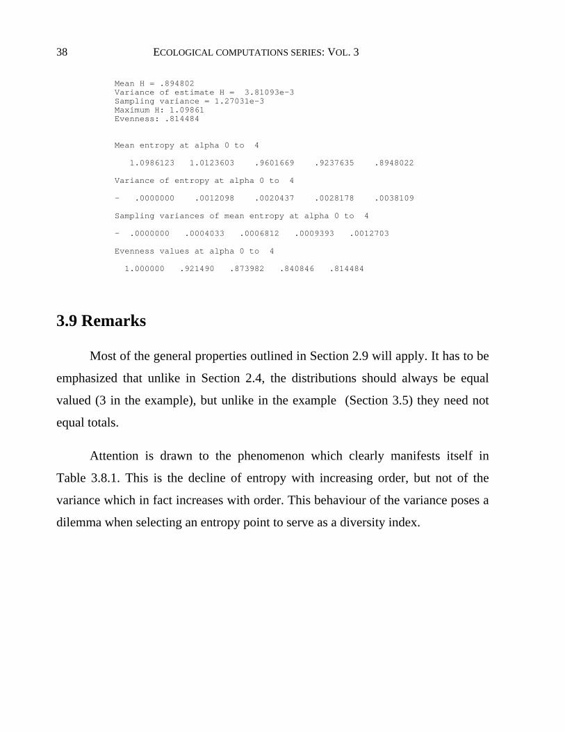
Mean H = .894802 Variance of estimate H = 3.81093e-3 Sampling variance = 1.27031e-3 Maximum H: 1.09861 Evenness: .814484 Mean entropy at alpha 0 to 4 1.0986123 1.0123603 .9601669 .9237635 .8948022 Variance of entropy at alpha 0 to 4 - .0000000 .0012098 .0020437 .0028178 .0038109 Sampling variances of mean entropy at alpha 0 to 4 - .0000000 .0004033 .0006812 .0009393 .0012703 Evenness values at alpha 0 to 4 1.000000 .921490 .873982 .840846 .814484

3.9 Remarks

Most of the general properties outlined in Section 2.9 will apply. It has to be

emphasized that unlike in Section 2.4, the distributions should always be equal

valued (3 in the example), but unlike in the example (Section 3.5) they need not

equal totals.

Attention is drawn to the phenomenon which clearly manifests itself in

Table 3.8.1. This is the decline of entropy with increasing order, but not of the

variance which in fact increases with order. This behaviour of the variance poses a

dilemma when selecting an entropy point to serve as a diversity index.

39

4 Information estimation Process sampling in k surges generates the frequencies. The information is

Rényi's (Eq. 1.5) and the averaging method is Pielou's.

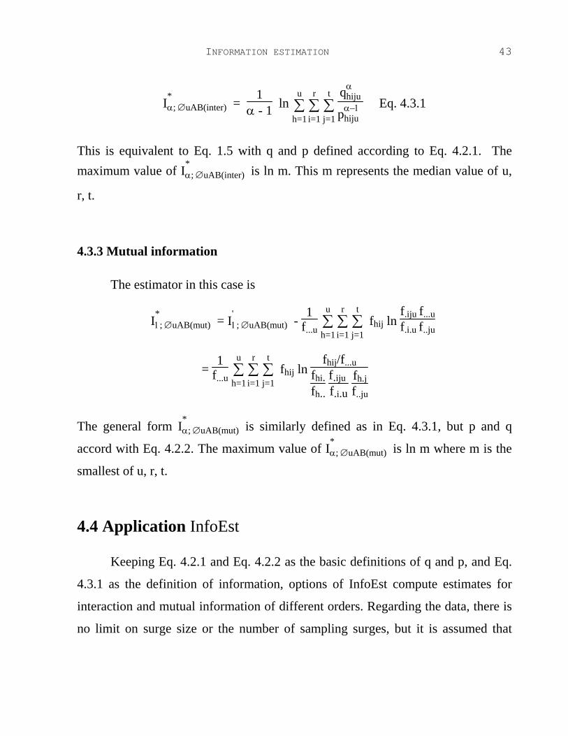
4.1 The data The frequencies are arranged in k r x t tables. In symbolic terms the hth of

the tables is

Table h B1 B2 ... Bt Total _____________________________________________ A1 fh11 fh12 ... fh1t fh1. A2 fh21 fh22 ... fh2t fh2. . . . ... . . Ar fhr1 fhr2 ... fhrt fhr. _____________________________________________ Total fh.1 fh.2 ... fh.t fh..


The following definitions of symbols apply:

r - number of categories, classification A.

t - number of categories, classification B.

k - number of sampling surges, the sampling process (classification C.) fhij - joint frequency of category i, classification A and category j, classification B

with category h, classification C. fhi. - joint frequency of category i, classification A and category h, classification

C. fh.j - joint frequency of category j, classification B and category h, classification

C. fh.. - frequency of category h, classification C.

4.2 Information

Information of order α is computed for two distributions

Q = (q1 q2 ... qs) and P = (p1 p2 ... ps)

Indirectly when the strength of association is measured there may be more than

two sets of classificatory criteria and a multidimensional joint distribution from

which the q and p quantities are derived. The exact definition of q and p will

depend on the perceived type of mutuality. If q and p are formulated as in

qhij = fhij f...

and phij = fh..f...

f.i. f...

f..jf...

Eq. 4.2.1

INFORMATION ESTIMATION 41

Iα of Eq. 1.5 will measure interaction information between classifications A,B,C. If

this information is of order 1, 2f.I1 will be Kullback's one-way information

divergence. If on the other hand q and p are formulated as in

qhij = fhij f...

and phij = fhi.fh..

f.ij f.i.

fh.jf..j Eq. 4.2.2

Iα will measure mutual information. The two types of mutuality are identified by

the shaded areas in Fig. 4.2.1.18

Fig. 4.2.1 Venn representation of interaction information (shaded area left) and mutual information (shaded area right) in a 3d frequency distribution. In terms of the example (Section 4.1) A,B are the row and column classifications and C the k-step sampling process.

4.3 Estimation

4.3.1 The averaging method

The data set is described in Section 4.1. There are k r x c tables and for each an information quantity IαhAB is computed. Following the logic outlined in Section

3.4, one possibility is to average information according to

18 See Abramson (1963).


I'α; ∅uAB(...) =

f1..I α1AB(...) + f2..I

α2AB(...) + ... + fu..I

αuAB(...)

f...u

which is equivalent to

I'α; ∅uAB(...) =

1(α - 1) f..u

∑h=1

u fh.j ln ∑

i=1

r ∑j=1

t

qαhij

pα−1hij

Since I'α; ∅uAB(...) does not incorporate shared information, one should opt for the

alternative quantity

I*α; ∅uAB(...) = I'

α; ∅uAB(...) + Iα; →uAB(shared)

The exact definition of I'α; ∅uAB(...) depends on the definition of q and p which in

turn depends on whether interaction or mutual information is wanted (see Section

4.2.)

4.3.1.1 Interaction information

The desired estimator of interaction information of order one, sampling

surge u, is given by

I*1; ∅uAB(inter) = I'

1; ∅uAB(inter) - 1

f...u ∑h=1

u ∑

i=1

r ∑j=1

t fhij ln

(f.i.u/f ...u)(f..ju/f

...u)(fhi./fh..)(fh.j/fh..)

= 1

f...u ∑h=1

u ∑

i=1

r ∑j=1

t fhij ln

fhij f2...u

fh..f.i.uf..ju

In general terms,


I*α; ∅uAB(inter) =

1α - 1 ln ∑

h=1

u ∑i=1

r ∑j=1

t qα

hiju

pα−1hiju

Eq. 4.3.1

This is equivalent to Eq. 1.5 with q and p defined according to Eq. 4.2.1. The maximum value of I*

α; ∅uAB(inter) is ln m. This m represents the median value of u,

r, t.

4.3.3 Mutual information

The estimator in this case is

I*1; ∅uAB(mut) = I'

1; ∅uAB(mut) - 1

f...u ∑h=1

u ∑i=1

r ∑j=1

t fhij ln

f.iju f...uf.i.u f..ju

= 1

f...u ∑h=1

u ∑i=1

r ∑j=1

t fhij ln

fhij/f...ufhi.fh..

f.iju f.i.u

fh.jf..ju

The general form I*α; ∅uAB(mut) is similarly defined as in Eq. 4.3.1, but p and q

accord with Eq. 4.2.2. The maximum value of I*α; ∅uAB(mut) is ln m where m is the

smallest of u, r, t.

4.4 Application InfoEst

Keeping Eq. 4.2.1 and Eq. 4.2.2 as the basic definitions of q and p, and Eq.

4.3.1 as the definition of information, options of InfoEst compute estimates for

interaction and mutual information of different orders. Regarding the data, there is

no limit on surge size or the number of sampling surges, but it is assumed that


surge size, table dimensions and classificatory criteria are kept intact as the

sampling proceeds.

4.5 Sample calculations

4.5.1 Interaction information

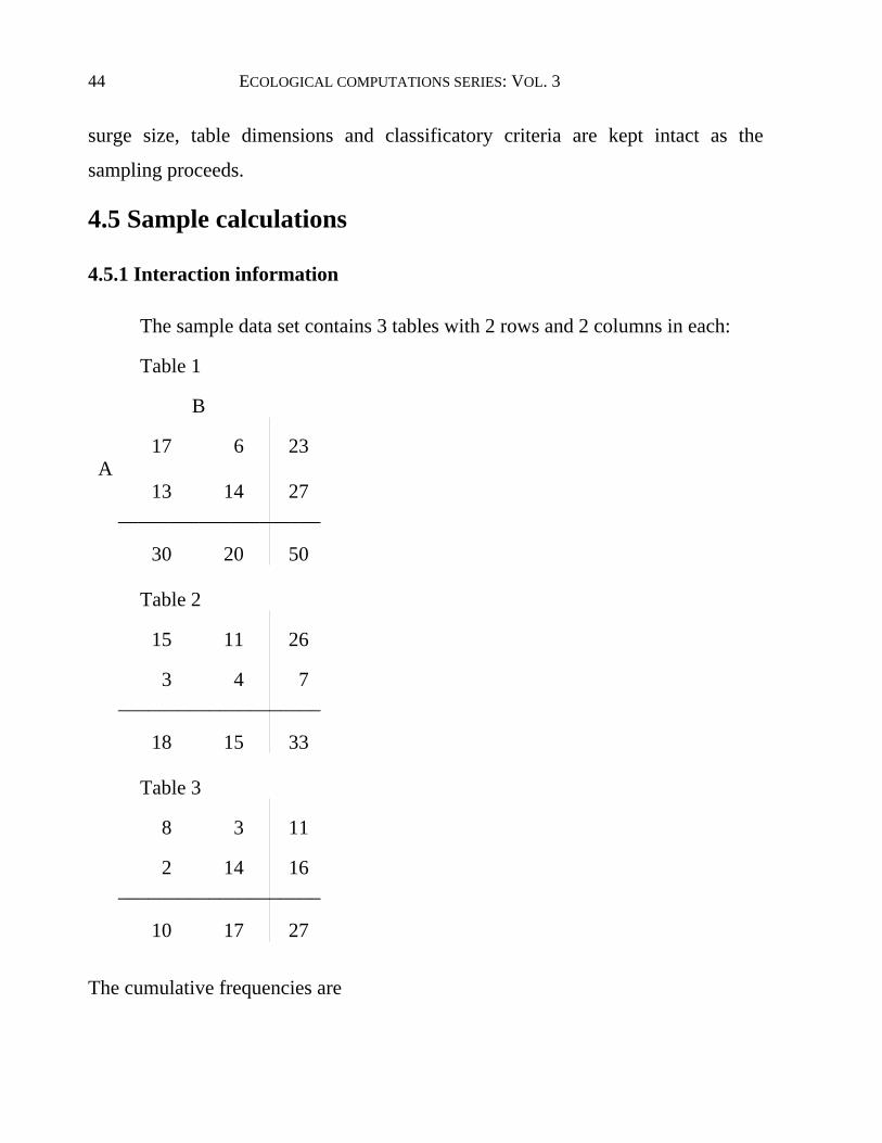
The sample data set contains 3 tables with 2 rows and 2 columns in each:

Table 1

B

17 6 23 A 13 14 27 ____________________

30 20 50 Table 2

15 11 26

3 4 7 ____________________

18 15 33 Table 3

8 3 11

2 14 16 ____________________

10 17 27

The cumulative frequencies are


32 17 49 16 18 34 ____________________ 48 35 83

for u = 2 and

40 20 60 18 32 50 ____________________ 58 52 110

for u=3. Recall that for interaction information (Eq. 4.3.1) q and p accord with Eq.

4.2.1 and proceed as follows:

1a. For u = 1,

q1111 = 17 50 p1111 =

5050

2350

3050

q1121 = 6

50 p1121 = 5050

2350

2050

q1211 = 13 50 p1211 =

5050

2750

3050

q1221 = 14 50 p1221 =

5050

2750

2050

I*1; ∅1AB(inter) = 0.035059

(within computer rounding errors.)

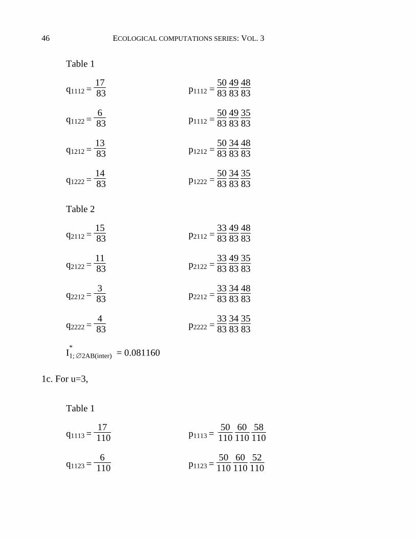
1b. For u=2 ,


Table 1

q1112 = 17 83 p1112 =

5083

4983

4883

q1122 = 6

83 p1112 = 5083

4983

3583

q1212 = 13 83 p1212 =

5083

3483

4883

q1222 = 14 83 p1222 =

5083

3483

3583

Table 2

q2112 = 15 83 p2112 =

3383

4983

4883

q2122 = 11 83 p2122 =

3383

4983

3583

q2212 = 3

83 p2212 = 3383

3483

4883

q2222 = 4

83 p2222 = 3383

3483

3583

I*1; ∅2AB(inter) = 0.081160

1c. For u=3,

Table 1

q1113 = 17

110 p1113 = 50110

60110

58110

q1123 = 6

110 p1123 = 50110

60110

52110


q1213 = 13

110 p1213 = 50110

50110

58110

q1223 = 14

110 p1223 = 50110

50110

52110

Table 2

q2113 = 15

110 p2113 = 33110

60110

58110

q2123 = 11

110 p2123 = 33110

60110

52110

q2213 = 3

110 p2213 = 33110

50110

58110

q2223 = 4

110 p2223 = 33110

50110

52110

Table 3

q3113 = 8

110 p3113 = 27110

60110

58110

q3123 = 3

110 p3123 = 27110

60110

52110

q3213 = 2

110 p3213 = 27110

50110

58110

q3223 = 14

110 p3223 = 27110

50110

52110

I*1; ∅3AB(inter) = 0.13827


2. With inflection point at IP, the estimated interaction information of order 1 is

computed according to

I 1; ∅uAB(inter) =

|f...u I*1; ∅uAB(inter) - f...u-1 I*

1; ∅u-1AB(inter)| f...u - f...u-1

u = IP+1, ..., k. For given IP = 1 and k = 3,

I 1; ∅2AB(inter) =

83 x 0.081160 - 50 x 0.035059 83 - 50 = 0.15101

I 1; ∅3AB(inter) = 0.31382

4. The average of the above is the estimated interaction information,

I 1;AB(inter) =

1k - IP ∑

u=IP+1

k I

1; ∅uAB(inter)

= 0.15101 + 0.31382

3 - 1

= 0.23242

5. The variance of the mean is

S21; AB(inter) =

1(k - IP)(k - IP - 1) ∑

u=IP+1

k (I

1; ∅uAB(inter) - I 1;AB(inter) )

2

= (0.15101 - 0.23242)2 + (0.31382 - 0.23242)2

(3 - 1)(3 - 1 -1)

= 0.0066268


Interaction information of any legitimate order is computed on the basis of the

same q and p values as above. Application InfoEst, option I, does the computations

automatically.

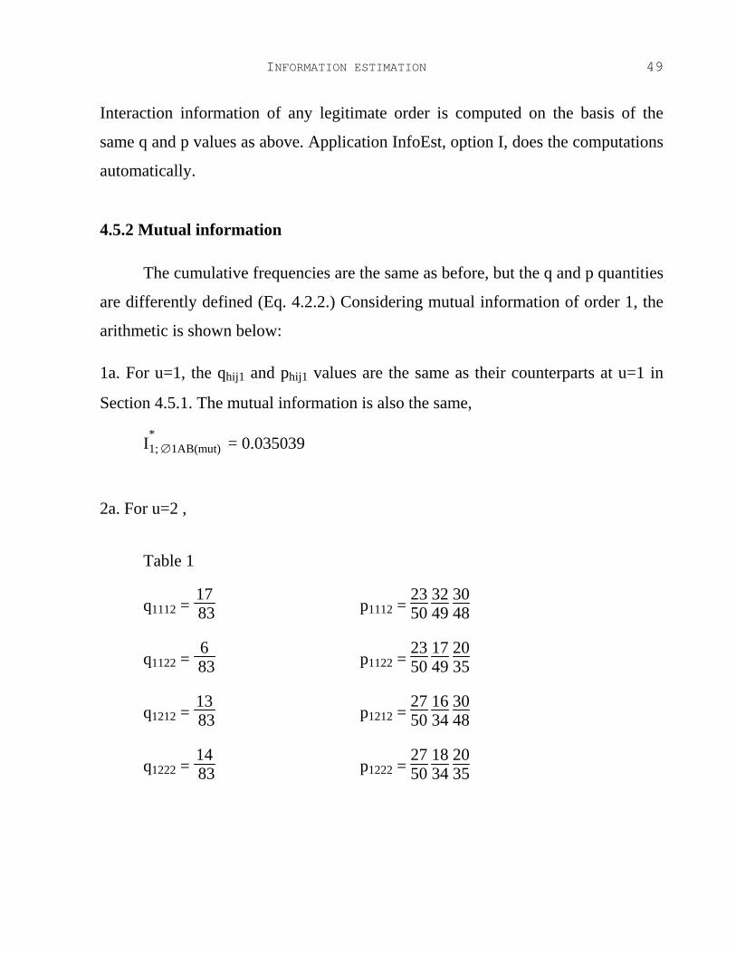
4.5.2 Mutual information

The cumulative frequencies are the same as before, but the q and p quantities

are differently defined (Eq. 4.2.2.) Considering mutual information of order 1, the

arithmetic is shown below:

1a. For u=1, the qhij1 and phij1 values are the same as their counterparts at u=1 in

Section 4.5.1. The mutual information is also the same,

I*1; ∅1AB(mut) = 0.035039

2a. For u=2 ,

Table 1

q1112 = 17 83 p1112 =

2350

3249

3048

q1122 = 6

83 p1122 = 2350

1749

2035

q1212 = 13 83 p1212 =

2750

1634

3048

q1222 = 14 83 p1222 =

2750

1834

2035


Table 2

q2112 = 15 83 p2112 =

2633

3249

1848

q2122 = 11 83 p2122 =

2633

1749

1535

q2212 = 3

83 p2212 = 733

1634

1848

q2222 = 4

83 p2222 = 733

1834

1535

I*1; ∅2AB(mut) = 0.0075568

2b. For u=3,

Table 1

q1113 = 17

110 p1113 = 2350

4060

3058

q1123 = 6

110 p1123 = 2350

2060

2052

q1213 = 13

110 p1213 = 2750

1850

3058

q1223 = 14

110 p1223 = 2750

3250

2052

Table 2

q2113 = 15

110 p2113 = 2633

4060

1858


q2123 = 11

110 p2123 = 2633

2060

1552

q2213 = 3

110 p2213 = 733

1850

1858

q2223 = 4

110 p2223 = 733

3250

1552

Table 3

q3113 = 8

110 p3113 = 1127

4060

1058

q3123 = 3

110 p3123 = 1127

2060

1752

q3213 = 2

110 p3213 = 1627

1850

1058

q3223 = 14

110 p3223 = 1627

3250

1752

I*1; ∅3AB(mut) = 0.019087

3. With inflection point at IP, the information estimates accord with

I 1; ∅uAB(mut) =

|f...u I*1; ∅uAB(mut) - f...u-1 I*

1; ∅u-1AB(mut)| f...u - f...u-1

for u = IP+1, ..., k. For given IP = 1 and k = 3,

I 1; ∅2AB(mut) =

|83 x 0.0075568 - 50 x 0.035039| 83 - 50 = 0.034113

I 1; ∅3AB(mut) = 0.054533


4. The average of the above values is the mutual information estimate sought,

I 1; AB(mut) =

1k - IP ∑

u=IP+1

k I

1; ∅uAB(mut) = 0.034113 + 0.054533

3 - 1

= 0.044323

5. The variance of the mean is

S21; AB(mut) =

1(k - IP)(k - IP - 1) ∑

u=IP+1

k (I

1; ∅uAB(mut) - I 1; AB(mut))

2

= (0.034113 - 0.044323)2 + (0.054533 - 0.044323)2

(3 - 1)(3 - 1 -1)

= 0.00010424

Use program InfoEst, option M, to compute estimates for mutual information of

any legitimate order.

4.6 More data

Sampling along 4 line transects across 3 elevation belts (500 - 1000 m, 1000

- 1500 m, 1500 - 2000 m) and 6 stratal groups (herb, fern, low shrub, high shrub,

evergreen tree, deciduous tree) yielded the following data:

Table 1 - North transect 0 2 11 0 0 0 3 9 5 2 0 0 1 3 8 1 1 1 Table 2 - East transect 1 6 6 3 1 2


0 3 10 1 1 0 2 10 4 0 1 0 Table 3 - South transect 2 1 12 0 1 1 1 5 6 2 1 0 0 1 12 2 0 0 Table 4 - West transect 1 7 6 0 2 1 0 0 9 1 2 1 1 6 8 4 0 0

Average frequencies determined from line intercepts are recorded. These are

entered on file (Frequency.dat) by row: 0 2 11 0 0 0 3 9 5 2 0 0 1 3 8 1 1 1 1 6


6 3 1 2 0 3 10 1 1 0 2 10 4 0 1 0 2 1 12 0 1 1 1 5 6 2 1 0 0 1 12 2 0 0 1 7 6 0 2


1 0 0 9 1 2 1 1 6 8 4 0 0

Recall that this type of file begins with a number and each number is followed by

an END-OF-PARAGRAPH mark created by pressing the RETURN key. Zeros are

legitimate in the data as long as at least one cell in any row or column of a table is

a non- zero value. No blanks are permitted.

4.7 Running InfoEst

After the data file is created, open a WORK folder and drag the ikons of

InfoEst and the data file (Frequency.dat) to this folder. Start up InfoEst from the

WORK folder by clicking twice on its ikon. The start-up dialogue is shown in Fig.

4.7.1 (interaction information) and in Fig. 4.7.3 (mutual information.) Observe

that:

1. If the application and data are not in same folder, respond on the 1st screen line

by pressing N (do not hit the RETURN key after N), otherwise press Y. Key N

stops the run while key Y allows it to continue.


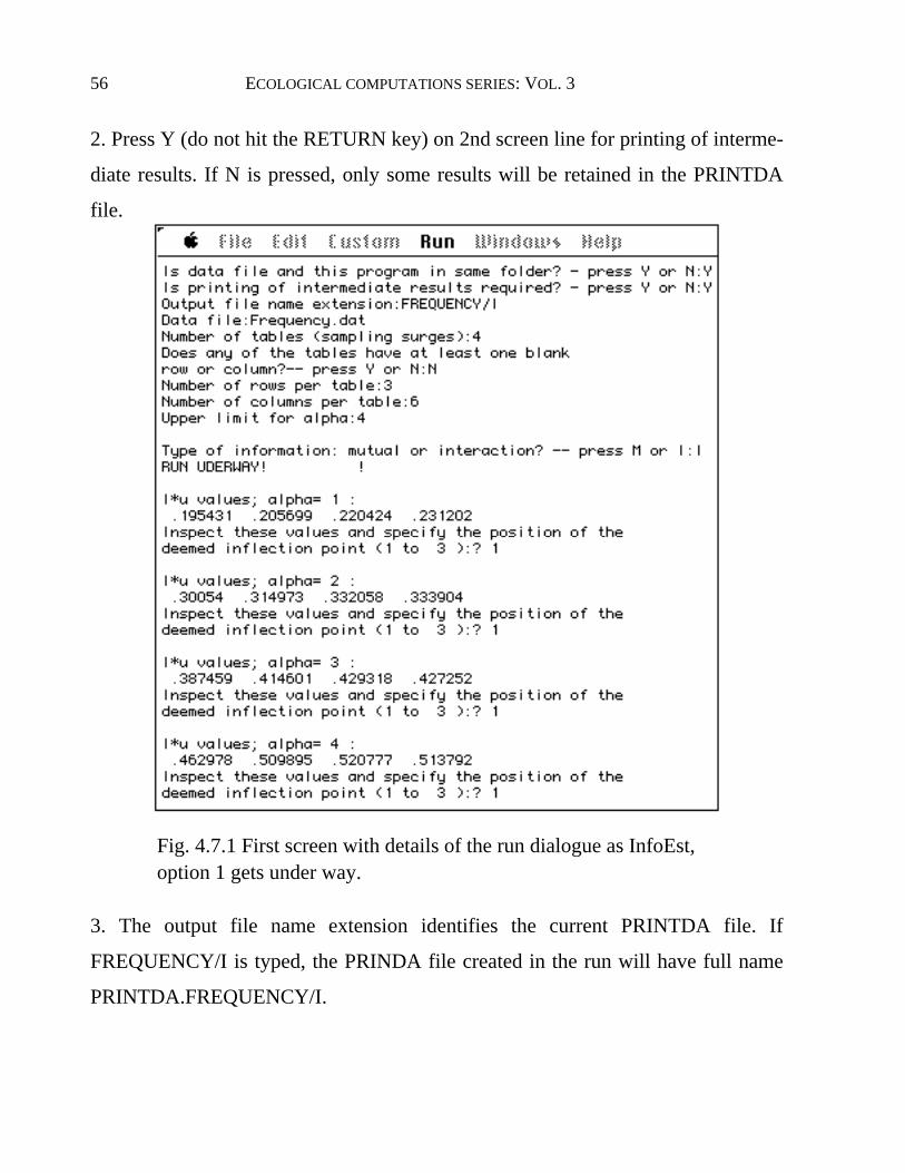
2. Press Y (do not hit the RETURN key) on 2nd screen line for printing of interme-

diate results. If N is pressed, only some results will be retained in the PRINTDA

file.

Fig. 4.7.1 First screen with details of the run dialogue as InfoEst, option 1 gets under way.

3. The output file name extension identifies the current PRINTDA file. If

FREQUENCY/I is typed, the PRINDA file created in the run will have full name

PRINTDA.FREQUENCY/I.


4. The data file is identified by its full name on the 4th screen line.

5. The number of tables is not limited.

6. Respond with N on the seventh screen line to abort the run if a blank row or a

blank column is present in a table (do not press the return key after pressing N.) If

Y is pressed, the run continues.

7. The number of table rows is invariant.

8. The number of table columns is invariant.

If fewer numbers are given in the data file then specified in the

start-up dialogue, or if blank lines are present in the data file,

the application will stop.

9. The upper limit for alpha (screen line 10) is freely chosen. The lower limit is

always 1 and the step size is also 1.

10. The type of information is either interaction (option I) or mutual (option M.)

11. The I*α; ∅uAB(inter) or I*

α; ∅uAB(mutual) values, as many in number as there are

successive frequency tables, are printed on the screen for each value of α and the

user is requested to pick a position which is deems to represent the main inflection

point.

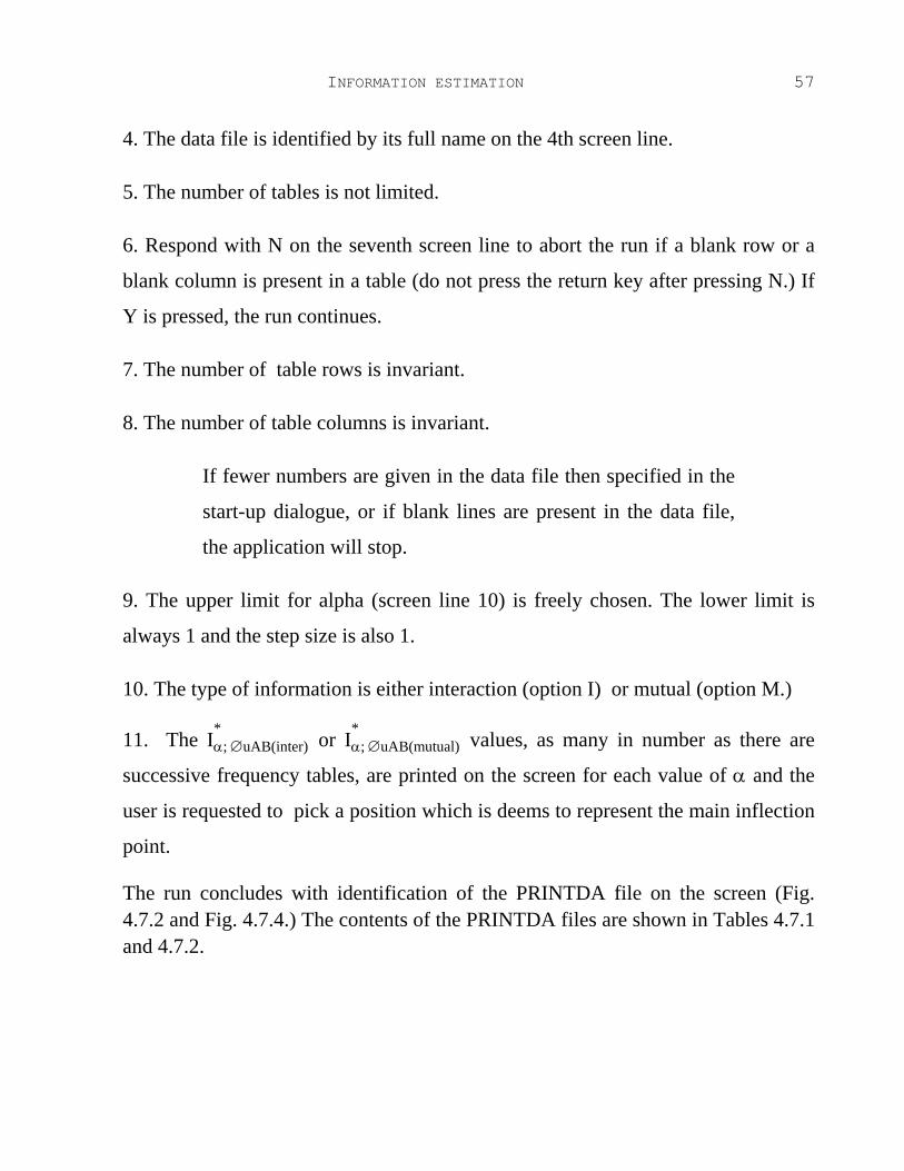
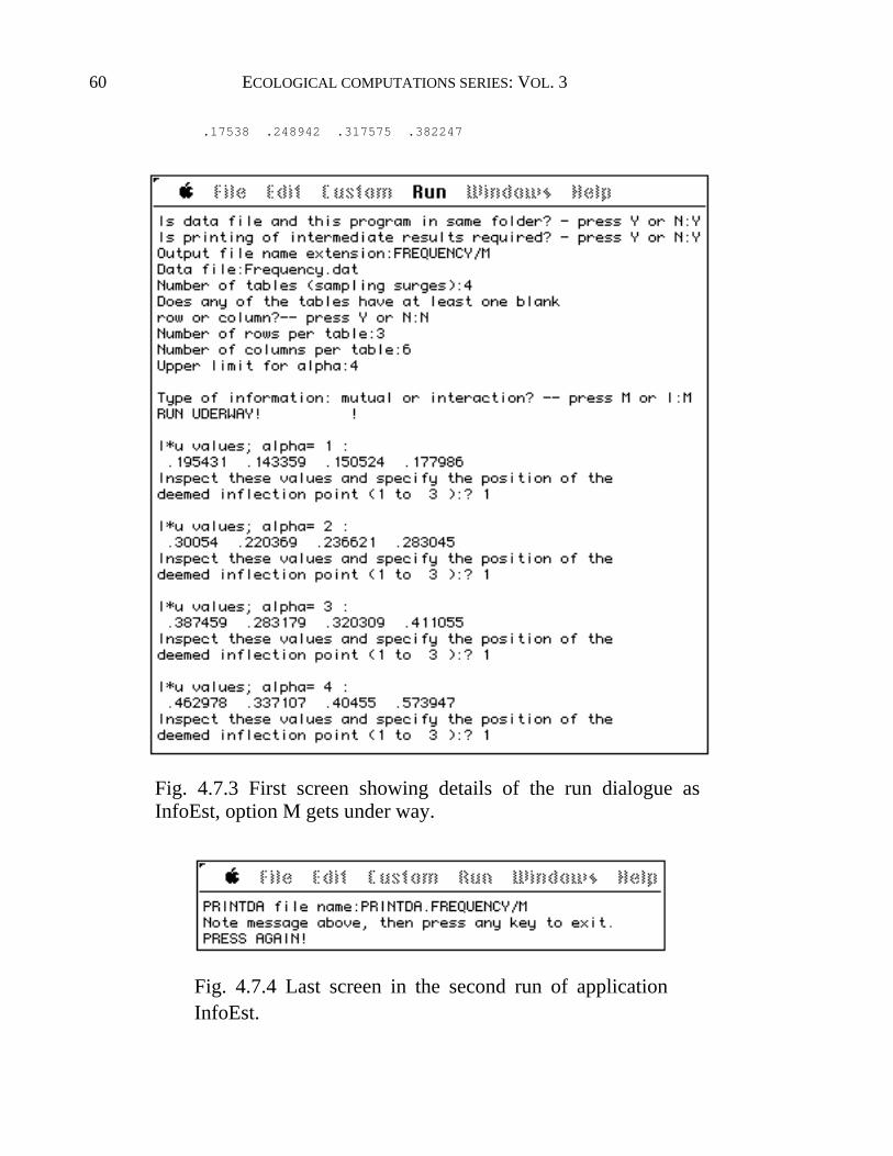
The run concludes with identification of the PRINTDA file on the screen (Fig. 4.7.2 and Fig. 4.7.4.) The contents of the PRINTDA files are shown in Tables 4.7.1 and 4.7.2.


Fig. 3.7.2 Last screen in a run of application InfoEst.

Table 4.7.1 Contents of file PRINTDA.FREQUENCY/I created in a run of application InfoEst, option I. PROGRAM InfoEst Interaction information computed for different alpha. Input data file:Frequency.dat Number of tables (sampling surges)= 4 Number of rows= 3 Number of columns= 6 DATA TABLE 1 0 2 11 0 0 0 3 9 5 2 0 0 1 3 8 1 1 1 TABLE 2 1 6 6 3 1 2 0 3 10 1 1 0 2 10 4 0 1 0 TABLE 3 2 1 12 0 1 1 1 5 6 2 1 0 0 1 12 2 0 0 TABLE 4 1 7 6 0 2 1 0 0 9 1 2 1 1 6 8 4 0 0 Table totals 47 51 47 49 Row totals 66 62 66 Column totals 12 53 97 16 10 6 I*u values; alpha= 1 .195431 .205699 .220424 .231202 Relevant Iu values for alpha= 1 in positions 1 and up: .195431 .215162 .251129 .263095


I*u values; alpha= 2 .30054 .314973 .332058 .333904 Relevant Iu values for alpha= 2 in positions 1 and up: .30054 .328273 .367682 .339367 I*u values; alpha= 3 .387459 .414601 .429318 .427252 Relevant Iu values for alpha= 3 in positions 1 and up: .387459 .439615 .460002 .421138 I*u values; alpha= 4 .462978 .509895 .520777 .513792 Relevant Iu values for alpha= 4 in positions 1 and up: .462978 .553132 .543468 .493123 alpha = 1 Inflexion point= 1 Mean I = .243128 Variance = 6.22405e-4 Sampling variance = 2.07468e-4 alpha = 2 Inflexion point= 1 Mean I = .345107 Variance = 4.12976e-4 Sampling variance = 1.37659e-4 alpha = 3 Inflexion point= 1 Mean I = .440252 Variance = 3.77915e-4 Sampling variance = 1.25972e-4 alpha = 4 Inflexion point= 1 Mean I = .529907 Variance = 1.03818e-3 Sampling variance = 3.46061e-4 Mean I for alpha=1 to 4 .243128 .345107 .440252 .529907 Variance of I for alpha=1 to 4 6.22405e-4 4.12976e-4 3.77915e-4 1.03818e-3 Sampling variance of I for alpha=1 to 4 2.07468e-4 1.37659e-4 1.25972e-4 3.46061e-4 Maximum I= 1.38629 Relative I for alpha=1 to 4


.17538 .248942 .317575 .382247

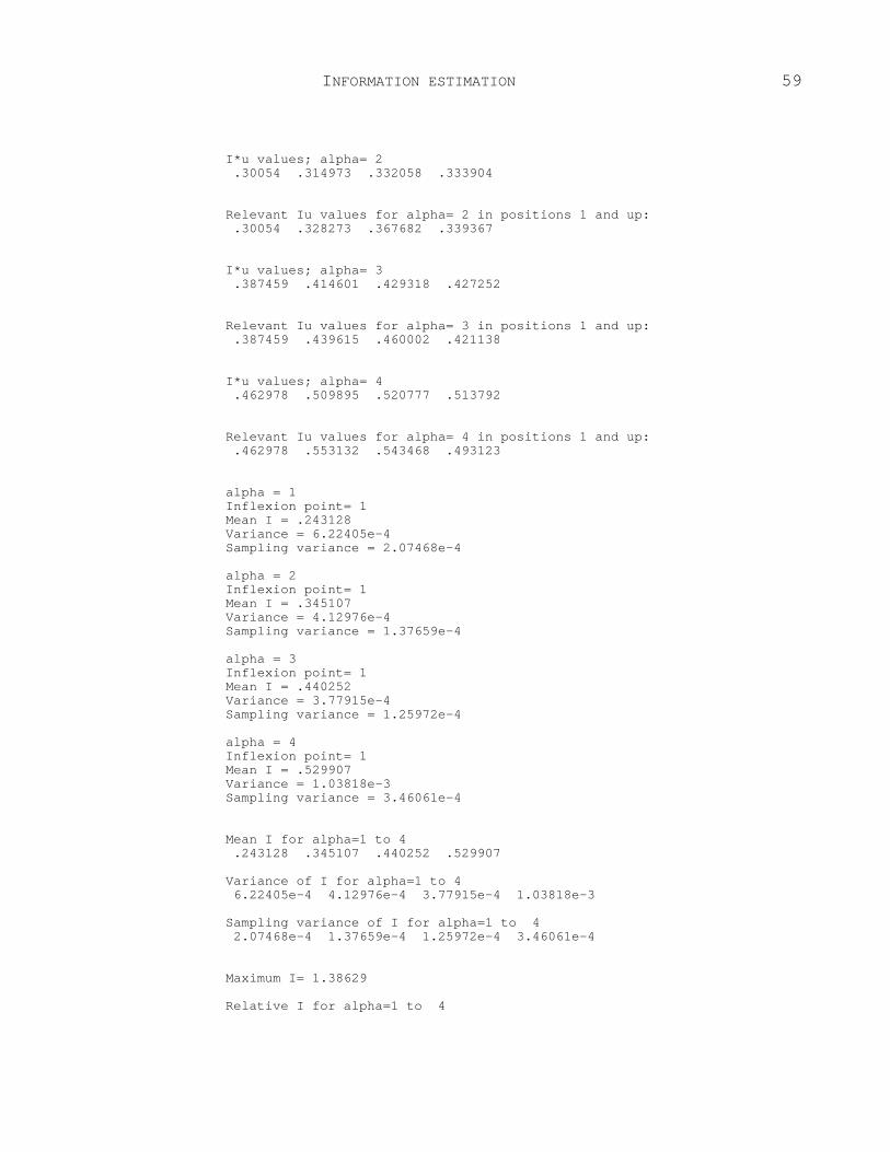
Fig. 4.7.3 First screen showing details of the run dialogue as InfoEst, option M gets under way.

Fig. 4.7.4 Last screen in the second run of application InfoEst.


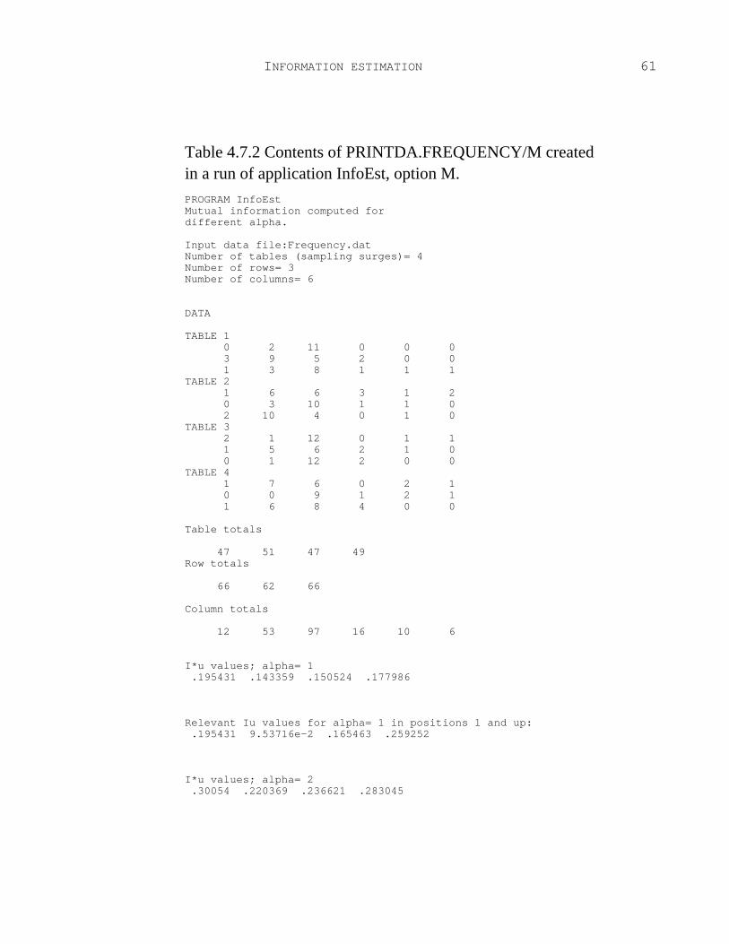
Table 4.7.2 Contents of PRINTDA.FREQUENCY/M created in a run of application InfoEst, option M.

PROGRAM InfoEst Mutual information computed for different alpha. Input data file:Frequency.dat Number of tables (sampling surges)= 4 Number of rows= 3 Number of columns= 6 DATA TABLE 1 0 2 11 0 0 0 3 9 5 2 0 0 1 3 8 1 1 1 TABLE 2 1 6 6 3 1 2 0 3 10 1 1 0 2 10 4 0 1 0 TABLE 3 2 1 12 0 1 1 1 5 6 2 1 0 0 1 12 2 0 0 TABLE 4 1 7 6 0 2 1 0 0 9 1 2 1 1 6 8 4 0 0 Table totals 47 51 47 49 Row totals 66 62 66 Column totals 12 53 97 16 10 6 I*u values; alpha= 1 .195431 .143359 .150524 .177986 Relevant Iu values for alpha= 1 in positions 1 and up: .195431 9.53716e-2 .165463 .259252 I*u values; alpha= 2 .30054 .220369 .236621 .283045


Relevant Iu values for alpha= 2 in positions 1 and up: .30054 .146487 .270506 .420423 I*u values; alpha= 3 .387459 .283179 .320309 .411055 Relevant Iu values for alpha= 3 in positions 1 and up: .387459 .187078 .397727 .679591 I*u values; alpha= 4 .462978 .337107 .40455 .573947 Relevant Iu values for alpha= 4 in positions 1 and up: .462978 .221108 .545176 1.07522 alpha = 1 Inflexion point= 1 Mean I = .173362 Variance = 6.76098e-3 Sampling variance = 2.25366e-3 alpha = 2 Inflexion point= 1 Mean I = .279139 Variance = 1.88162e-2 Sampling variance = 6.27207e-3 alpha = 3 Inflexion point= 1 Mean I = .421466 Variance = 6.10648e-2 Sampling variance = 2.03549e-2 alpha = 4 Inflexion point= 1 Mean I = .613835 Variance = .185914 Sampling variance = 6.19713e-2 Mean I for alpha=1 to 4 .173362 .279139 .421466 .613835 Variance of I for alpha=1 to 4 6.76098e-3 1.88162e-2 6.10648e-2 .185914 Sampling variance of I for alpha=1 to 4 2.25366e-3 6.27207e-3 2.03549e-2 6.19713e-2 Maximum I= 1.09861 Relative I for alpha=1 to 4 .157801 .254083 .383635 .558737


4.8 Remarks

The properties outlined in Section 2.9 apply to the marginal distributions and

the joint distribution. There are also new properties:

1. The mutual information is a more restrictive descriptor of relationships than the

interaction information. The interaction information cannot be less than the mutual

information.

2. Whereas entropy in the marginal and joint distributions has a descending trend

with increasing α, information (mutual or interaction) has an ascending trend. In

all cases the variance increases with increasing α.

3. Both mutual and interaction information of order 1 have statistical meaning

under Kullback's definition of MDIS. InfoEst estimates information of different

orders; this allows flexibility in the characterizations of the data.

4. To pass from Rényi's I of order 1 to Kullback's MDIS, multiply the former by

twice the grand total of the tables. For example, a relevant estimate in Table 4.7.1 is I1 = 0.243128 or in relative terms 0.243128/ln 4 = 0.175379 (also in Table

4.7.1.) The relevant grand total of the frequencies is 147 (last 3 tables in Table

4.7.1.) The corresponding MDIS quantity is 0.243128 x 2 x 147 = 71.480 which

has 20 degrees of freedom. The possible maximum MDIS is 2 x ln 4 x 147 = 407.570 and the relative MDIS is the same as the relative I1. The latter indicates a

rather weak relationship.

64

Glossary accuracy -- closeness to the true value.

ASCII -- a standard sorting order for characters; a coding system used in computer

work, e.g., ASCII code 77 identifies the capital letter M.

biological type -- the organism's strategy by which it survives the unfavourable

season; also life-form. bit -- the unit of entropy; log2 2 is one bit.

community -- here a plant assemblage structured by types and interactions.

diversity -- the number or richness of alternatives; usually expressed as a logarithm

of proportions.

disorder -- a state of reduced predictability; diversity.

distribution -- an arrangement of events or objects between types.

entropy -- information per observation; the level of disorder; surprisal value.

GLOSSARY 65

equivocation -- the portion that is specific; the opposite of mutual; information in

one distribution not repeated in another.

evenness -- the closeness to an equi-distribution.

information -- a multiple of entropy; a logarithmic measure of mutuality or

equivocation; a divergence or equivocation.

interaction -- here an analytical property measurable as information.

MDIS -- Kullback's information theoretical measure on which his brand of

statistics is based; a one-way divergence measured as the logarithm of the ratio

of proportions.

mutual -- not specific; shared.

population -- a collection of events of the same generic type characterized by a

frequency distribution; a collection of organisms characterized by common

inheritance.

process sampling -- sampling in surges with intermittent analyses to monitor the

evolution of specific internal sample properties and their environmental

connections.

sample -- a subset of the population.

sampling -- the act of selecting units for measurement.

sampling surge -- a step in process sampling.

species richness -- the number of species in a community; the logarithm of this

number; state richness.

state richness -- a property of distributions; the logarithm of the number of states;

species richness.

surge size -- sample size per step in process sampling.

66

Bibliography Brillouin, L. 1962. Science and Information Theory. Academic Press, New York.

Abramson, N. 1963. Information Theory and Coding. McGraw-Hill, New York.

Edgington, E. S. 1987. Randomization Tests. 2nd ed. Marcel Dekker, New York.

Feoli, E., M. Lagonegro and L. Orlóci. 1984. Information Analysis of Vegetation

Data. Dr. W. Junk, bv., The Hague.

Hawking, S. W. 1988. A brief History of Time. Bantam Books, New York.

Hill, O. H. 1973. Diversity and evenness: a unifying notion and its consequences.

Ecology 54: 427-432.

BIBLIOGRAPHY 67

Juhász-Nagy, P. and J. Podani. 1983. Information theory methods for the study of

spatial processes and succession. Vegetatio 51: 129-140.

Kenkel, N. C., Juhász-Nagy P. and Podani, J. 1989. On sampling procedures in

population and community ecology. Vegetatio 83:195-207.

Kullback, S. 1968. Information Theory and Statistics. Dover Publications, New

York.

Margalef, D. R. 1958. Information theory in ecology. Yearbook of the Society for

General Systems Research 3: 36-71.

Margalef, D. R. 1989. On diversity and connectivity, as historical expressions of

ecosystems. COENOSES 4:121-126.

Orlóci, L. 1969. Information analysis of structure in biological collections. Nature

223: 483-484.

Orlóci, L. 1978. Multivariate Analysis in Vegetation Research. 2nd ed. Dr. W.

Junk, The Hague.

Orlóci, L. 1988. Community organization: recent advances in numerical methods.

Can. J. Bot. 66:2626-2633.

Orlóci, L. and W. Stanek. 1980. Vegetation survey of the Alaska Highway, Yukon

territory: types and gradients. Vegetatio 41:1-56.

Orlóci, L. and Pillar, V. De Patta. 1990. On sample size optimality in ecosystem

survey. Biometrie-Praximetrie 29:173-184.


Orlóci, L. and Pillar, V. De Patta. 1990. Ecosystem surveys: When to stop

sampling. Proceedings of the 1989 International Conference and Workshop on

Global Monitoring and Assessment: Preparing for the 21st Century, Venice.

Fondacione G. Gini, Rome.

Pielou, E. C. 1966. Shannon's formula as a measure of species diversity: its use and

misuse. Amer. Natur. 100: 463-465.

Pielou, E. C. 1974. Population and Community Ecology. Gordon and Breach

Science Publishers, New York.

Pielou, E. C. 1975. Ecological Diversity. Wiley, New York.

Pielou, E. C. 1977. Mathematical Ecology. 2nd ed. Wiley, New York.

Podani, J. 1998. Spatial processes in the analysis of vegetation: theory and review.

Acta Botanica Hungarica 30: 75-118.

Poore, M. E. D. 1955. The use of phytosociological methods in ecological

investigations. II. Practical issues involved in an attempt to apply the Braun-

Blanquet system. J. Ecol. 43:226-244.

Poore, M. E. D. 1956. The use of phytosociological methods in ecological

investigations. III. Practical applications. J. Ecol. 40:28-50.

Rényi, A. 1961. On measures of entropy and information. In: J. Neyman (ed.),

Proceedings of the 4th Berkeley Symposium on Mathematical Statistics and

Probability, pp. 547-561. University of California Press, Berkeley.

BIBLIOGRAPHY 69

Rajski, C. 1961. Entropy and metric spaces. In: C. Chery (ed.), Information

Theory, pp. 41-45. Butterworths, London.

Sampford, M. R. 1962. An Introduction to Sampling Theory. Oliver & Boyd,

Edinburgh.

Shannon, C. E. 1948. A mathematical theory of communication. Bell System Tech.

J. 27: 379-423.

Shannon, C. E. and W. Weaver. 1964. The Mathematical Theory of

communication. Univ. of Illinois Press, Urbana.

Wildi, O. and L. Orlóci. 1987. Flexible gradient analysis: a note on ideas and an

example. COENOSES 2:61-65.

Yockey, H. P., R. L. Platzman and H. Quastler (eds.) 1958. Information Theory in

Biology. Pergamon Press, New York.

Three main topics are covered: diversity graphs, entropy estimation,

information estimation. Concepts are discussed, methods described and step-by-

step examples presented. A synopsis of the program package INFOPACK is given

and the run dialogue is explained. The presentations assume program

implementation on a Macintosh. Book and programs are directed to users

interested in diversity theory and research.

Documents

ENTROPY AND INFORMATION - Publishpublish.uwo.ca/~lorloci/Koa/20 Information.pdf · O. Wildi & L. Orlóci Volume 2 ECOLOGICAL PROGRAMS FOR INSTRUCTIONAL COMPUTING ON THE MACINTOSH