Entropy and Complexity in Music: Some examples

byBarbra Gregory

A thesis submitted to the faculty of the University of North Carolina at Chapel Hill in partial ful-fillment of the requirements for the degree of Master of Science in the Department of Mathematics.

Chapel Hill2005

Approved by

Advisor: Professor Karl Petersen

Reader: Professor Sue Goodman

Reader: Professor Jane Hawkins

ABSTRACT

BARBRA GREGORY: Entropy and Complexity in Music: Some examples

(Under the direction of Professor Karl Petersen)

We examine the concepts of complexity and entropy and their application to musical structures

and explore the difficulty of obtaining a conclusive measure of entropy for a musical system. A set

of tools is applied to examples from modern composers, classical Western music, and traditional

tribal customs. Ergodic theory techniques are used to find the entropy of musical performance

structures left up to chance or choice. Techniques set forth by Lempel and Ziv, Pressing, and

Lerdahl and Jackendoff to explore the complexity of rhythms are studied and applied. Finally, we

consider the complexity of linguistic structure on a series of notes, first by counting the patterns

that are allowed within that structure and then by defining a new measure of complexity inspired

by the work of Pressing.

ii

ACKNOWLEDGMENTS

I would like to thank Dr. Thomas H. Brylawski of the University of North Carolina at Chapel

Hill for his help with Proposition 4.1.5. Dr. Thomas Warburton and Dr. Sarah Weiss of the

Department of Music at the University of North Carolina at Chapel Hill also provided useful

support throughout this work.

Thank you also to my advisor Karl Petersen who was adventurous enough to explore music and

mathematics with me.

And to Josh who kept telling me that this thesis could and would get done.

iii

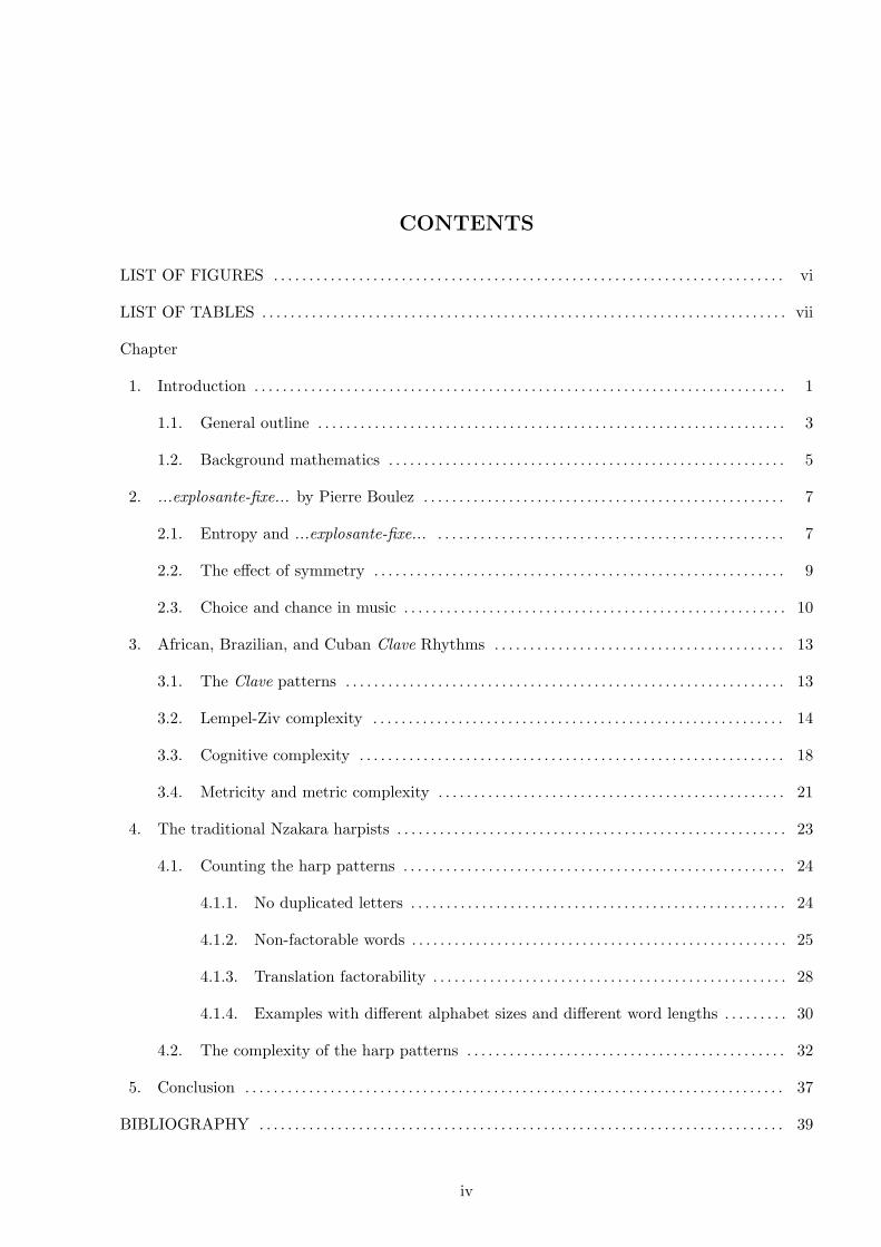
CONTENTS

LIST OF FIGURES . . . . . . . . . . . . . . . . . . . . . . . . . . . . . . . . . . . . . . . . . . . . . . . . . . . . . . . . . . . . . . . . . . . . . . . . vi

LIST OF TABLES . . . . . . . . . . . . . . . . . . . . . . . . . . . . . . . . . . . . . . . . . . . . . . . . . . . . . . . . . . . . . . . . . . . . . . . . . . vii

Chapter

1. Introduction . . . . . . . . . . . . . . . . . . . . . . . . . . . . . . . . . . . . . . . . . . . . . . . . . . . . . . . . . . . . . . . . . . . . . . . . . . . 1

1.1. General outline . . . . . . . . . . . . . . . . . . . . . . . . . . . . . . . . . . . . . . . . . . . . . . . . . . . . . . . . . . . . . . . . . . 3

1.2. Background mathematics . . . . . . . . . . . . . . . . . . . . . . . . . . . . . . . . . . . . . . . . . . . . . . . . . . . . . . . . 5

2. ...explosante-fixe... by Pierre Boulez . . . . . . . . . . . . . . . . . . . . . . . . . . . . . . . . . . . . . . . . . . . . . . . . . . . 7

2.1. Entropy and ...explosante-fixe... . . . . . . . . . . . . . . . . . . . . . . . . . . . . . . . . . . . . . . . . . . . . . . . . . 7

2.2. The effect of symmetry . . . . . . . . . . . . . . . . . . . . . . . . . . . . . . . . . . . . . . . . . . . . . . . . . . . . . . . . . . 9

2.3. Choice and chance in music . . . . . . . . . . . . . . . . . . . . . . . . . . . . . . . . . . . . . . . . . . . . . . . . . . . . . . 10

3. African, Brazilian, and Cuban Clave Rhythms . . . . . . . . . . . . . . . . . . . . . . . . . . . . . . . . . . . . . . . . . 13

3.1. The Clave patterns . . . . . . . . . . . . . . . . . . . . . . . . . . . . . . . . . . . . . . . . . . . . . . . . . . . . . . . . . . . . . . 13

3.2. Lempel-Ziv complexity . . . . . . . . . . . . . . . . . . . . . . . . . . . . . . . . . . . . . . . . . . . . . . . . . . . . . . . . . . 14

3.3. Cognitive complexity . . . . . . . . . . . . . . . . . . . . . . . . . . . . . . . . . . . . . . . . . . . . . . . . . . . . . . . . . . . . 18

3.4. Metricity and metric complexity . . . . . . . . . . . . . . . . . . . . . . . . . . . . . . . . . . . . . . . . . . . . . . . . . 21

4. The traditional Nzakara harpists . . . . . . . . . . . . . . . . . . . . . . . . . . . . . . . . . . . . . . . . . . . . . . . . . . . . . . . 23

4.1. Counting the harp patterns . . . . . . . . . . . . . . . . . . . . . . . . . . . . . . . . . . . . . . . . . . . . . . . . . . . . . . 24

4.1.1. No duplicated letters . . . . . . . . . . . . . . . . . . . . . . . . . . . . . . . . . . . . . . . . . . . . . . . . . . . . . 24

4.1.2. Non-factorable words . . . . . . . . . . . . . . . . . . . . . . . . . . . . . . . . . . . . . . . . . . . . . . . . . . . . . 25

4.1.3. Translation factorability . . . . . . . . . . . . . . . . . . . . . . . . . . . . . . . . . . . . . . . . . . . . . . . . . . 28

4.1.4. Examples with different alphabet sizes and different word lengths . . . . . . . . . 30

4.2. The complexity of the harp patterns . . . . . . . . . . . . . . . . . . . . . . . . . . . . . . . . . . . . . . . . . . . . . 32

5. Conclusion . . . . . . . . . . . . . . . . . . . . . . . . . . . . . . . . . . . . . . . . . . . . . . . . . . . . . . . . . . . . . . . . . . . . . . . . . . . . 37

BIBLIOGRAPHY . . . . . . . . . . . . . . . . . . . . . . . . . . . . . . . . . . . . . . . . . . . . . . . . . . . . . . . . . . . . . . . . . . . . . . . . . . 39

iv

LIST OF FIGURES

Figure 2.1. ...explosante-fixe... . . . . . . . . . . . . . . . . . . . . . . . . . . . . . . . . . . . . . . . . . . . . . . . . . . . . . . . . 7

Figure 2.2. Relabelling the graph of ...explosante-fixe... . . . . . . . . . . . . . . . . . . . . . . . . . . . . . . . . . 8

Figure 2.3. Composition with radial symmetry . . . . . . . . . . . . . . . . . . . . . . . . . . . . . . . . . . . . . . . . . . 10

Figure 2.4. Probability vectors for Musikalisches Wurfelspiel . . . . . . . . . . . . . . . . . . . . . . . . . . . . 12

Figure 4.1. The five allowable bichords of the Nzakara harpists . . . . . . . . . . . . . . . . . . . . . . . . . . 24

Figure 4.2. Example of a limanza canon . . . . . . . . . . . . . . . . . . . . . . . . . . . . . . . . . . . . . . . . . . . . . . . . 24

Figure 4.3. The five allowable bichords of the Nzakara harpists . . . . . . . . . . . . . . . . . . . . . . . . . . 32

v

LIST OF TABLES

Table 3.1. The Clave rhythms . . . . . . . . . . . . . . . . . . . . . . . . . . . . . . . . . . . . . . . . . . . . . . . . . . . . . . . . . . . 13

Table 3.2. The Lempel-Ziv complexity measures of the six Clave rhythms . . . . . . . . . . . . . . . . 15

Table 3.3. Types of syncopation in Pressing’s cognitive complexity Measure . . . . . . . . . . . . . . 19

Table 3.4. Calculation of the cognitive complexity of four-pulse rhythms . . . . . . . . . . . . . . . . . 20

Table 3.5. Cognitive complexities of the six Clave rhythms . . . . . . . . . . . . . . . . . . . . . . . . . . . . . . . 20

Table 3.6. Complexity measures of the six Clave rhythms . . . . . . . . . . . . . . . . . . . . . . . . . . . . . . . . 21

Table 3.7. Cognitive and metric complexities of the four-pulse rhythms . . . . . . . . . . . . . . . . . . 22

Table 4.1. Notation and Terminology . . . . . . . . . . . . . . . . . . . . . . . . . . . . . . . . . . . . . . . . . . . . . . . . . . . . 25

Table 4.2. The effect of Nzakara harp grammar in Z3 . . . . . . . . . . . . . . . . . . . . . . . . . . . . . . . . . . . . 31

Table 4.3. The effect of Nzakara harp grammar in Z5 . . . . . . . . . . . . . . . . . . . . . . . . . . . . . . . . . . . . 31

Table 4.4. The effect of Nzakara harp grammar in Z7 . . . . . . . . . . . . . . . . . . . . . . . . . . . . . . . . . . . . 31

Table 4.5. The computed complexities of selected bichord patterns . . . . . . . . . . . . . . . . . . . . . . . 36

vi

CHAPTER 1

Introduction

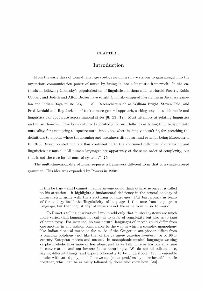
From the early days of formal language study, researchers have striven to gain insight into the

mysterious communication power of music by fitting it into a linguistic framework. In the en-

thusiasm following Chomsky’s popularization of linguistics, authors such as Harold Powers, Robin

Cooper, and Judith and Alton Becker have sought Chomsky-inspired hierarchies in Javanese game-

lan and Indian Raga music [23, 11, 3]. Researchers such as William Bright, Steven Feld, and

Fred Lerdahl and Ray Jackendoff took a more general approach, seeking ways in which music and

linguistics can cooperate across musical styles [6, 13, 18]. Most attempts at relating linguistics

and music, however, have been criticized repeatedly for such fallacies as failing fully to appreciate

musicality, for attempting to squeeze music into a box where it simply doesn’t fit, for stretching the

definitions to a point where the meaning and usefulness disappear, and even for being Eurocentric.

In 1975, Ruwet pointed out one flaw contributing to the continued difficulty of quantizing and

linguisticizing music: “All human languages are apparently of the same order of complexity, but

that is not the case for all musical systems.” [26]

The multi-dimensionality of music requires a framework different from that of a single-layered

grammar. This idea was expanded by Powers in 1980:

If this be true – and I cannot imagine anyone would think otherwise once it is calledto his attention – it highlights a fundamental deficiency in the general analogy ofmusical structuring with the structuring of languages. Put barbarously in termsof the analogy itself, the ‘linguisticity’ of languages is the same from language tolanguage, but the ‘linguisticity’ of musics is not the same from music to music.

To Ruwet’s telling observation I would add only that musical systems are muchmore varied than languages not only as to order of complexity but also as to kindof complexity. For instance, no two natural languages of speech could differ fromone another in any fashion comparable to the way in which a complex monophonylike Indian classical music or the music of the Gregorian antiphoner differs froma complex polphony (sic) like that of the Javanese gamelan klenengan or of 16th-century European motets and masses. In monophonic musical languages we singor play melodic lines more or less alone, just as we talk more or less one at a timein conversation, and our hearers follow accordingly. We do not all talk at once,saying different things, and expect coherently to be understood. Yet in ensemblemusics with varied polyphonic lines we can (so to speak) easily make beautiful musictogether, which can be as easily followed by those who know how. [24]

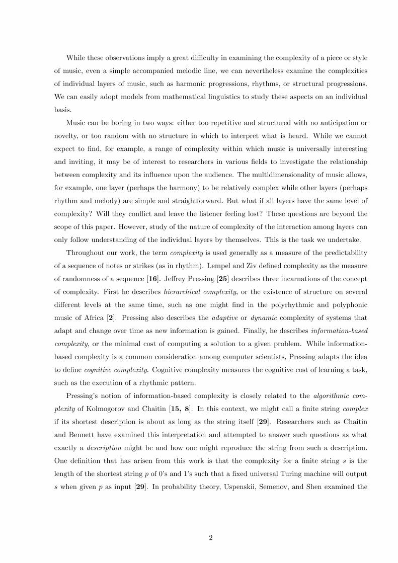
While these observations imply a great difficulty in examining the complexity of a piece or style

of music, even a simple accompanied melodic line, we can nevertheless examine the complexities

of individual layers of music, such as harmonic progressions, rhythms, or structural progressions.

We can easily adopt models from mathematical linguistics to study these aspects on an individual

basis.

Music can be boring in two ways: either too repetitive and structured with no anticipation or

novelty, or too random with no structure in which to interpret what is heard. While we cannot

expect to find, for example, a range of complexity within which music is universally interesting

and inviting, it may be of interest to researchers in various fields to investigate the relationship

between complexity and its influence upon the audience. The multidimensionality of music allows,

for example, one layer (perhaps the harmony) to be relatively complex while other layers (perhaps

rhythm and melody) are simple and straightforward. But what if all layers have the same level of

complexity? Will they conflict and leave the listener feeling lost? These questions are beyond the

scope of this paper. However, study of the nature of complexity of the interaction among layers can

only follow understanding of the individual layers by themselves. This is the task we undertake.

Throughout our work, the term complexity is used generally as a measure of the predictability

of a sequence of notes or strikes (as in rhythm). Lempel and Ziv defined complexity as the measure

of randomness of a sequence [16]. Jeffrey Pressing [25] describes three incarnations of the concept

of complexity. First he describes hierarchical complexity, or the existence of structure on several

different levels at the same time, such as one might find in the polyrhythmic and polyphonic

music of Africa [2]. Pressing also describes the adaptive or dynamic complexity of systems that

adapt and change over time as new information is gained. Finally, he describes information-based

complexity, or the minimal cost of computing a solution to a given problem. While information-

based complexity is a common consideration among computer scientists, Pressing adapts the idea

to define cognitive complexity. Cognitive complexity measures the cognitive cost of learning a task,

such as the execution of a rhythmic pattern.

Pressing’s notion of information-based complexity is closely related to the algorithmic com-

plexity of Kolmogorov and Chaitin [15, 8]. In this context, we might call a finite string complex

if its shortest description is about as long as the string itself [29]. Researchers such as Chaitin

and Bennett have examined this interpretation and attempted to answer such questions as what

exactly a description might be and how one might reproduce the string from such a description.

One definition that has arisen from this work is that the complexity for a finite string s is the

length of the shortest string p of 0’s and 1’s such that a fixed universal Turing machine will output

s when given p as input [29]. In probability theory, Uspenskii, Semenov, and Shen examined the

2

idea of randomness [?]. In doing so, they discuss some of the relations among randomness, com-

plexity, stochasticity, and entropy. Other notions of complexity arise fields as cellular automata,

information theory, statistical inference, ergodic theory, and dynamical systems [29].

Entropy, as used in information theory, measures the complexity of a sequence by measuring

the amount of unexpectedness of each symbol (or pitch or pulse), or, in other words, the amount

of information conveyed with each new element of the sequence [22]. Alternatively, one might

consider the entropy of a message to be the theoretical smallest number of bytes which can convey

the entire meaning of the message [22]. According to [7], topological entropy is “the exponential

growth rate of the number of essentially different orbit segments of length n” and measures “the

complexity of the orbit structure of a dynamical system.” More simply, [12] defines entropy as the

“rate at which information can be gleaned about a dynamical system from a sequence of repeated

observations” and [20] describes the topological entropy of a symbolic dynamical system as the

amount of freedom to concatenate words and remain within the system. We will consider many

incarnations of complexity and entropy: the richness of a language as a function of the constraints

put upon it and the consequent size of the vocabulary as in the case of the Nzakara harpists; the

unpredictability of a sequence as in the study of ...explosante-fixe..., or the Lempel-Ziv complexity

of the Clave rhythm patterns; or the amount of mental processing required to perform or hear

sequences as in the cognitive complexity measures of the rhythms and the complexity measure of

the harp patterns proposed by the author.

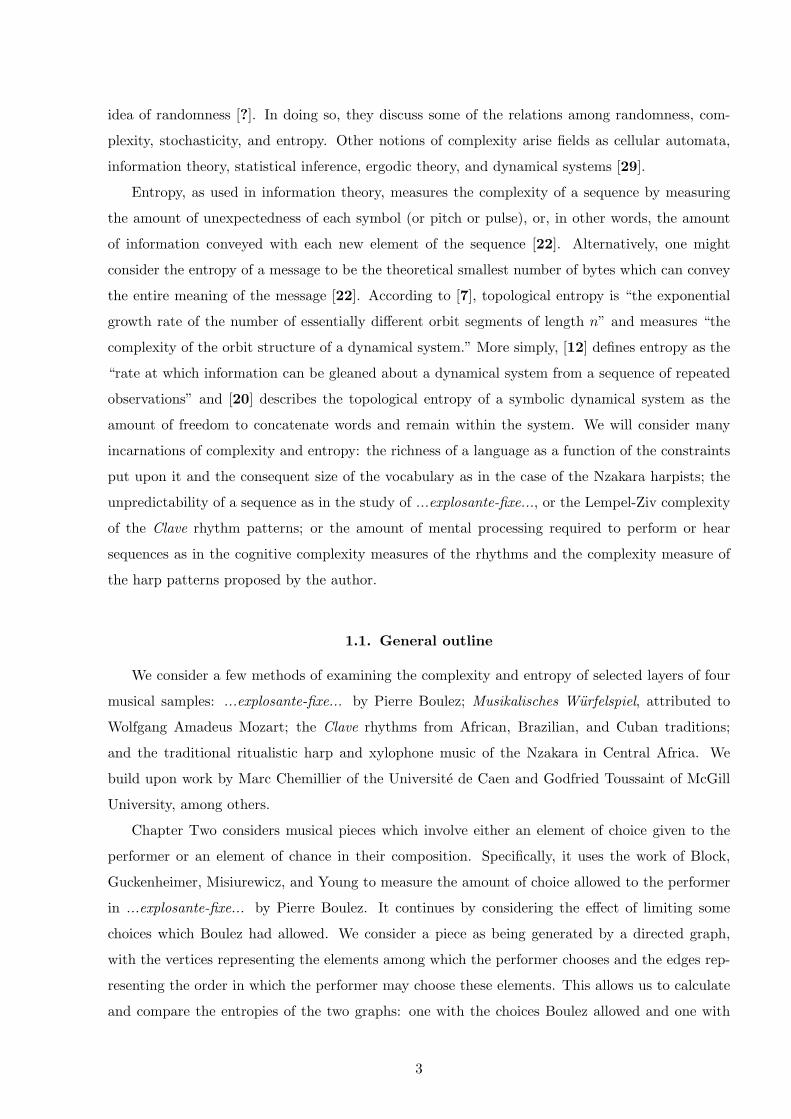
1.1. General outline

We consider a few methods of examining the complexity and entropy of selected layers of four

musical samples: ...explosante-fixe... by Pierre Boulez; Musikalisches Wurfelspiel, attributed to

Wolfgang Amadeus Mozart; the Clave rhythms from African, Brazilian, and Cuban traditions;

and the traditional ritualistic harp and xylophone music of the Nzakara in Central Africa. We

build upon work by Marc Chemillier of the Universite de Caen and Godfried Toussaint of McGill

University, among others.

Chapter Two considers musical pieces which involve either an element of choice given to the

performer or an element of chance in their composition. Specifically, it uses the work of Block,

Guckenheimer, Misiurewicz, and Young to measure the amount of choice allowed to the performer

in ...explosante-fixe... by Pierre Boulez. It continues by considering the effect of limiting some

choices which Boulez had allowed. We consider a piece as being generated by a directed graph,

with the vertices representing the elements among which the performer chooses and the edges rep-

resenting the order in which the performer may choose these elements. This allows us to calculate

and compare the entropies of the two graphs: one with the choices Boulez allowed and one with

3

two of those choices removed. We find that, as expected, decreasing the number of choices in-

creases the predictability of the performance. The chapter concludes with a discussion of Mozart’s

Musikalisches Wurfelspiel, in which the player “composes” a piece of music by rolling a pair of

dice to determine which of eleven prescribed choices to play at each of 16 measures. It is unclear

whether Mozart understood that different outcomes on the dice have different probabilities (for

example, rolling a seven is more common than rolling any other number). In this section, we find

that rolling dice gives a slightly more predictable result than if we were to draw one of the eleven

measures out of a hat with equal probability.

Chapter Three is based upon the work of Godfried Toussaint of McGill University in Montreal.

It continues his 2002 examination of the Clave rhythms of Cuba, Brazil, and Africa. Toussaint used

the work of Lempel and Ziv, Lerdahl and Jackendoff, and Jeffrey Pressing to quantify the relative

difficulty of each of six basic Clave rhythms. Here we review the work of Toussaint, consider

differences of interpretation of the original authors, and present some possible modifications of

Toussaint’s methods. We expand upon Toussaint’s use of the Lempel-Ziv algorithm to include an

alternative common parsing algorithm. We discuss the use of each of these parsings in calculations

of entropy and their most common modern usage in data compression. While the Lempel-Ziv

algorithms do not provide much information on the complexity of these relatively short rhythm

patterns, we find that the entropy of these patterns is zero, as should be true of any infinite cyclic

sequence. Further, we readapt the complexities defined by Lerdahl and Jackendoff and by Pressing

to compare the two in their ranking of the difficulty of the six rhythms.

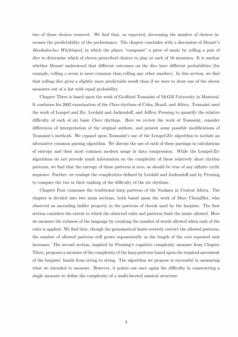
Chapter Four examines the traditional harp patterns of the Nzakara in Central Africa. The

chapter is divided into two main sections, both based upon the work of Marc Chemillier, who

observed an ascending ladder property in the patterns of chords used by the harpists. The first

section considers the extent to which the observed rules and patterns limit the music allowed. Here

we measure the richness of the language by counting the number of words allowed when each of the

rules is applied. We find that, though the grammatical limits severely restrict the allowed patterns,

the number of allowed patterns still grows exponentially as the length of the core repeated unit

increases. The second section, inspired by Pressing’s cognitive complexity measure from Chapter

Three, proposes a measure of the complexity of the harp patterns based upon the required movement

of the harpists’ hands from string to string. The algorithm we propose is successful in measuring

what we intended to measure. However, it points out once again the difficulty in constructing a

single measure to define the complexity of a multi-faceted musical structure.

4

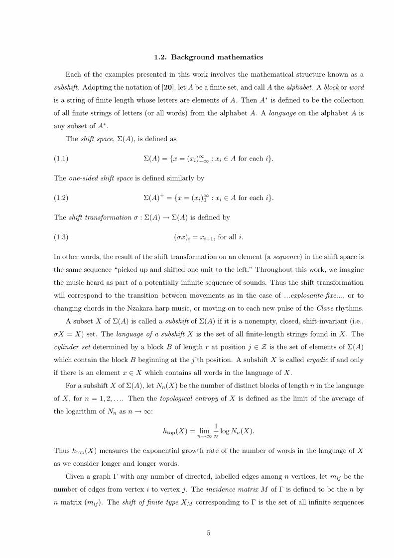
1.2. Background mathematics

Each of the examples presented in this work involves the mathematical structure known as a

subshift. Adopting the notation of [20], let A be a finite set, and call A the alphabet. A block or word

is a string of finite length whose letters are elements of A. Then A∗ is defined to be the collection

of all finite strings of letters (or all words) from the alphabet A. A language on the alphabet A is

any subset of A∗.

The shift space, Σ(A), is defined as

(1.1) Σ(A) = {x = (xi)∞−∞ : xi ∈ A for each i}.

The one-sided shift space is defined similarly by

(1.2) Σ(A)+ = {x = (xi)∞0 : xi ∈ A for each i}.

The shift transformation σ : Σ(A) → Σ(A) is defined by

(1.3) (σx)i = xi+1, for all i.

In other words, the result of the shift transformation on an element (a sequence) in the shift space is

the same sequence “picked up and shifted one unit to the left.” Throughout this work, we imagine

the music heard as part of a potentially infinite sequence of sounds. Thus the shift transformation

will correspond to the transition between movements as in the case of ...explosante-fixe..., or to

changing chords in the Nzakara harp music, or moving on to each new pulse of the Clave rhythms.

A subset X of Σ(A) is called a subshift of Σ(A) if it is a nonempty, closed, shift-invariant (i.e.,

σX = X) set. The language of a subshift X is the set of all finite-length strings found in X. The

cylinder set determined by a block B of length r at position j ∈ Z is the set of elements of Σ(A)

which contain the block B beginning at the j’th position. A subshift X is called ergodic if and only

if there is an element x ∈ X which contains all words in the language of X.

For a subshift X of Σ(A), let Nn(X) be the number of distinct blocks of length n in the language

of X, for n = 1, 2, . . .. Then the topological entropy of X is defined as the limit of the average of

the logarithm of Nn as n →∞:

htop(X) = limn→∞

1n

log Nn(X).

Thus htop(X) measures the exponential growth rate of the number of words in the language of X

as we consider longer and longer words.

Given a graph Γ with any number of directed, labelled edges among n vertices, let mij be the

number of edges from vertex i to vertex j. The incidence matrix M of Γ is defined to be the n by

n matrix (mij). The shift of finite type XM corresponding to Γ is the set of all infinite sequences

5

whose letters are the labels on the edges of Γ and whose spellings are determined by following the

edges in order around the graph. It is straightforward to show that M2 is the matrix whose ij’th

entry gives the number of two-step paths between vertex i and vertex j, and in general Mk gives

the number of k-step paths. The topological entropy of the system is given by

htop(XM ) = limn→∞

1n

log2 (number of n-blocks in XM ) = limn→∞

1n

log2

∑i,j

(Mn)ij = log2 λM ,

where λM is the largest positive eigenvalue of M [19, 20].

6

CHAPTER 2

...explosante-fixe... by Pierre Boulez

In the 1970s, mathematician-turned-composer Pierre Boulez wrote ...explosante-fixe... in honor

of the late Igor Stravinsky. ...explosante-fixe..., in both its original form and its current form

following major revisions in the 1990s, challenges traditional ideas of chamber music and makes

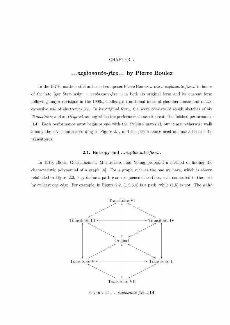
extensive use of electronics [5]. In its original form, the score consists of rough sketches of six

Transitoires and an Originel, among which the performers choose to create the finished performance

[14]. Each performance must begin or end with the Originel material, but it may otherwise walk

among the seven units according to Figure 2.1, and the performance need not use all six of the

transitoires.

2.1. Entropy and ...explosante-fixe...

In 1979, Block, Guckenheimer, Misiurewicz, and Young proposed a method of finding the

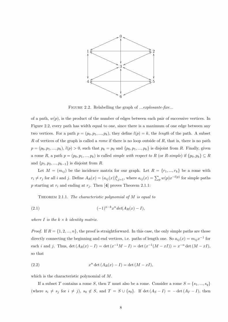
characteristic polynomial of a graph [4]. For a graph such as the one we have, which is shown

relabelled in Figure 2.2, they define a path p as a sequence of vertices, each connected to the next

by at least one edge. For example, in Figure 2.2, (1,2,3,4) is a path, while (1,5) is not. The width

Transitoire VI77

wwooooooooooooooooo gg

''OOOOOOOOOOOOOOOOOOO

��

Transitoire IIIOO

��

oo //gg

''NNNNNNNNNNNNNNNNN Transitoire IVOO

��

77

wwppppppppppppppppp

Originel77

wwppppppppppppppppp gg

''NNNNNNNNNNNNNNNNNOO

��

Transitoire Vgg

''OOOOOOOOOOOOOOOOOoo // Transitoire II77

wwooooooooooooooooo

Transitoire VII

Figure 2.1. ...explosante-fixe...[14]

066

vvnnnnnnnnnnnnnnnnn hh

((PPPPPPPPPPPPPPPPPOO

��

1OO

��

oo //hh

((PPPPPPPPPPPPPPPPP 2OO

��

66

vvnnnnnnnnnnnnnnnnn

366

vvnnnnnnnnnnnnnnnnn hh

((PPPPPPPPPPPPPPPPPOO

��

4 hh

((PPPPPPPPPPPPPPPPPoo // 566

vvnnnnnnnnnnnnnnnnn

6

Figure 2.2. Relabelling the graph of ...explosante-fixe...

of a path, w(p), is the product of the number of edges between each pair of successive vertices. In

Figure 2.2, every path has width equal to one, since there is a maximum of one edge between any

two vertices. For a path p = (p0, p1, ..., pk), they define l(p) = k, the length of the path. A subset

R of vertices of the graph is called a rome if there is no loop outside of R, that is, there is no path

p = (p0, p1, ..., pk), l(p) > 0, such that pk = p0 and {p0, p1, ..., pk} is disjoint from R. Finally, given

a rome R, a path p = (p0, p1, ..., pk) is called simple with respect to R (or R-simple) if {p0, pk} ⊆ R

and {p1, p2, ..., pk−1} is disjoint from R.

Let M = (mij) be the incidence matrix for our graph. Let R = {r1, ..., rk} be a rome with

ri 6= rj for all i and j. Define AR(x) = (aij(x))ki,j=1, where aij(x) =

∑p w(p)x−l(p) for simple paths

p starting at ri and ending at rj . Then [4] proves Theorem 2.1.1:

Theorem 2.1.1. The characteristic polynomial of M is equal to

(2.1) (−1)n−kxndet(AR(x)− I),

where I is the k × k identity matrix.

Proof. If R = {1, 2, ..., n}, the proof is straightforward. In this case, the only simple paths are those

directly connecting the beginning and end vertices, i.e. paths of length one. So aij(x) = mijx−1 for

each i and j. Thus, det (AR(x)− I) = det (x−1M − I) = det (x−1(M − xI)) = x−n det (M − xI),

so that

(2.2) xn det (AR(x)− I) = det (M − xI),

which is the characteristic polynomial of M .

If a subset T contains a rome S, then T must also be a rome. Consider a rome S = {s1, ..., sq}

(where si 6= sj for i 6= j), s0 6∈ S, and T = S ∪ {s0}. If det (AS − I) = −det (AT − I), then

8

xn det (AS − I) = −xn det (AT − I), and the principle of induction can be used to prove the theorem

by starting with the rome R = {1, ..., n} and reducing the size of the rome by one at each step.

If AS−I = (bij)qi,j=1 and AT−I = (cij)

qi,j=0, then by the definition of AS and AT , bij = cij+ci0c0j

since every S-simple path from si to sj will either be a T -simple path or will be a combination

of two T -simple paths, one from si to s0 and the other from s0 to sj . Since S is a rome and s0

is not in S, there can be no paths from s0 to itself which are T -simple. So c00 = −1, since all

T -simple paths from s0 to itself will have length 0. By a series of column operations, we transform

the matrix AT − I into a matrix D = (dij)qi,j=0 with dij = bij for i, j > 0, d00 = −1, and d0j = 0

for j > 0. Namely, we multiply the 0’th column of AT − I by c0j and add it to the j’th column of

AT − I for j = 1, ..., q. Basic linear algebra then tells us that det (dij)qi,j=0 = det (AT − I). Then

since dij = bij for i, j > 0, det (AS − I) = −det (dij)qi,j=0 = −det (AT − I), as desired. ♦

Consider, in Figure 2.2, the rome R = 1, 2, 3, 4, 5. Then AR(x) is as in Equation (2.3):

(2.3) AR(x) =

x−2 x−1 + x−2 x−1 + x−2 x−1 0

x−1 + x−2 x−2 x−1 + x−2 0 x−1

x−1 + x−2 x−1 + x−2 2x−2 x−1 + x−2 x−1 + x−2

x−1 0 x−1 + x−2 x−2 x−1 + x−2

0 x−1 x−1 + x−2 x−1 + x−2 x−2

Using Mathematica combined with Theorem 2.1.1, the characteristic polynomial of this graph

is given by −1− 16x− 40x2− 16x3 +20x4 +14x5. Again using Mathematica, the largest eigenvalue

of this system is approximately 4.15633, and by [19] and [4], the entropy of this system is given by

h = log2 4.15633 ≈ 2.0553.

To compute the entropy directly, let M = (mij) be the incidence matrix for the graph in

Figure 2.2. Then the ij’th entry of the matrix Mn is the number of paths of length n from vertex

i − 1 to vertex j − 1 in the graph. If the sum of the entries of Mn is given by mn, the entropy of

the graph is h = limn→∞ n−1 log2 mn [20]. Again we find using Mathematica that the entropy of

the graph is approximately equal to 2.0553.

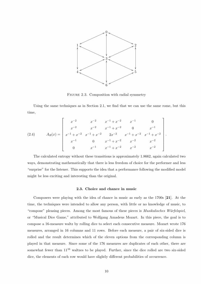
2.2. The effect of symmetry

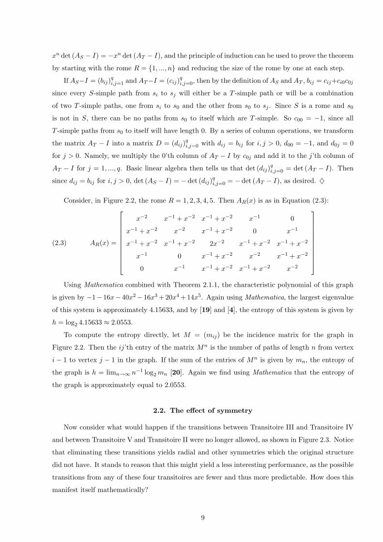
Now consider what would happen if the transitions between Transitoire III and Transitoire IV

and between Transitoire V and Transitoire II were no longer allowed, as shown in Figure 2.3. Notice

that eliminating these transitions yields radial and other symmetries which the original structure

did not have. It stands to reason that this might yield a less interesting performance, as the possible

transitions from any of these four transitoires are fewer and thus more predictable. How does this

manifest itself mathematically?

9

066

vvnnnnnnnnnnnnnnnnn hh

((PPPPPPPPPPPPPPPPPOO

��

1OO

��

hh

((PPPPPPPPPPPPPPPPP 2OO

��

66

vvnnnnnnnnnnnnnnnnn

366

vvnnnnnnnnnnnnnnnnn hh

((PPPPPPPPPPPPPPPPPOO

��

4 hh

((PPPPPPPPPPPPPPPPP 566

vvnnnnnnnnnnnnnnnnn

6

Figure 2.3. Composition with radial symmetry

Using the same techniques as in Section 2.1, we find that we can use the same rome, but this

time,

(2.4) AR(x) =

x−2 x−2 x−1 + x−2 x−1 0

x−2 x−2 x−1 + x−2 0 x−1

x−1 + x−2 x−1 + x−2 2x−2 x−1 + x−2 x−1 + x−2

x−1 0 x−1 + x−2 x−2 x−2

0 x−1 x−1 + x−2 x−2 x−2

.

The calculated entropy without these transitions is approximately 1.8662, again calculated two

ways, demonstrating mathematically that there is less freedom of choice for the performer and less

“surprise” for the listener. This supports the idea that a performance following the modified model

might be less exciting and interesting than the original.

2.3. Choice and chance in music

Composers were playing with the idea of chance in music as early as the 1700s [21]. At the

time, the techniques were intended to allow any person, with little or no knowledge of music, to

“compose” pleasing pieces. Among the most famous of these pieces is Musikalisches Wurfelspiel,

or “Musical Dice Game,” attributed to Wolfgang Amadeus Mozart. In this piece, the goal is to

compose a 16-measure waltz by rolling dice to select each consecutive measure. Mozart wrote 176

measures, arranged in 16 columns and 11 rows. Before each measure, a pair of six-sided dice is

rolled and the result determines which of the eleven options from the corresponding column is

played in that measure. Since some of the 176 measures are duplicates of each other, there are

somewhat fewer than 1116 waltzes to be played. Further, since the dice rolled are two six-sided

dice, the elements of each row would have slightly different probabilities of occurrence.

10

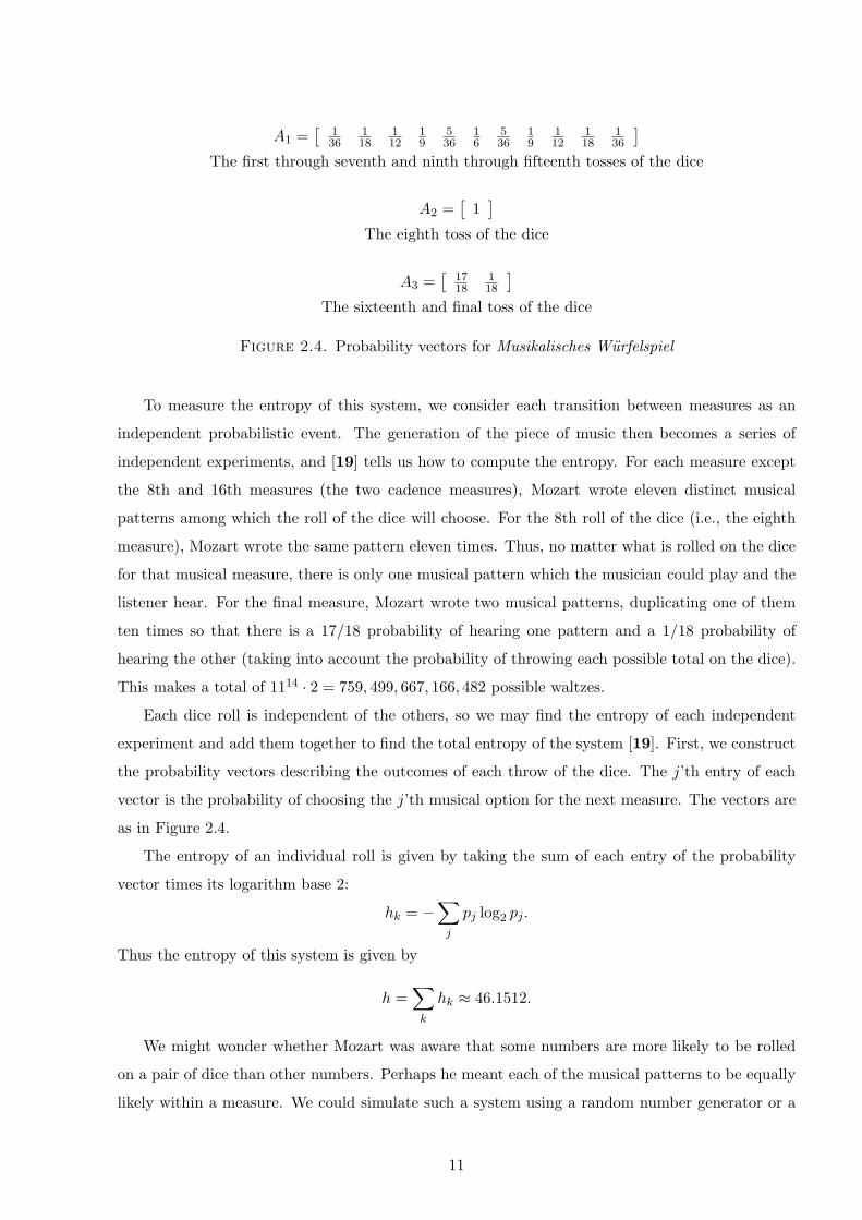
A1 =[

136

118

112

19

536

16

536

19

112

118

136

]The first through seventh and ninth through fifteenth tosses of the dice

A2 =[

1]

The eighth toss of the dice

A3 =[

1718

118

]The sixteenth and final toss of the dice

Figure 2.4. Probability vectors for Musikalisches Wurfelspiel

To measure the entropy of this system, we consider each transition between measures as an

independent probabilistic event. The generation of the piece of music then becomes a series of

independent experiments, and [19] tells us how to compute the entropy. For each measure except

the 8th and 16th measures (the two cadence measures), Mozart wrote eleven distinct musical

patterns among which the roll of the dice will choose. For the 8th roll of the dice (i.e., the eighth

measure), Mozart wrote the same pattern eleven times. Thus, no matter what is rolled on the dice

for that musical measure, there is only one musical pattern which the musician could play and the

listener hear. For the final measure, Mozart wrote two musical patterns, duplicating one of them

ten times so that there is a 17/18 probability of hearing one pattern and a 1/18 probability of

hearing the other (taking into account the probability of throwing each possible total on the dice).

This makes a total of 1114 · 2 = 759, 499, 667, 166, 482 possible waltzes.

Each dice roll is independent of the others, so we may find the entropy of each independent

experiment and add them together to find the total entropy of the system [19]. First, we construct

the probability vectors describing the outcomes of each throw of the dice. The j’th entry of each

vector is the probability of choosing the j’th musical option for the next measure. The vectors are

as in Figure 2.4.

The entropy of an individual roll is given by taking the sum of each entry of the probability

vector times its logarithm base 2:

hk = −∑

j

pj log2 pj .

Thus the entropy of this system is given by

h =∑

k

hk ≈ 46.1512.

We might wonder whether Mozart was aware that some numbers are more likely to be rolled

on a pair of dice than other numbers. Perhaps he meant each of the musical patterns to be equally

likely within a measure. We could simulate such a system using a random number generator or a

11

single eleven-sided die. In such a case, the entropy of the system would be

h = log2 (1114 · 2) ≈ 49.431 [19].

The entropy of this completely random system is 1.07 times the entropy of the original system.

Thus Mozart limited by a small amount the unexpectedness of each measure. Had Mozart wanted

to maximize the amount of unexpectedness at each measure, he should have instructed the musician

to pull a number 1 through 11 out of a hat at each measure rather than rolling two dice.

12

CHAPTER 3

African, Brazilian, and Cuban Clave Rhythms

In the summer of 2002, Godfried Toussaint presented an analysis of the complexity of six Clave

rhythms [28]. He chose three methods of analysis proposed by earlier authors and compared the

results of his experiments to the difficulty students report experiencing in learning each of these

rhythms. This section presents his methods and results along with some proposed modifications to

the procedure.

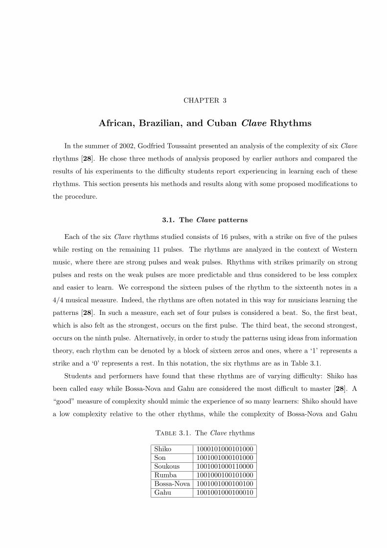
3.1. The Clave patterns

Each of the six Clave rhythms studied consists of 16 pulses, with a strike on five of the pulses

while resting on the remaining 11 pulses. The rhythms are analyzed in the context of Western

music, where there are strong pulses and weak pulses. Rhythms with strikes primarily on strong

pulses and rests on the weak pulses are more predictable and thus considered to be less complex

and easier to learn. We correspond the sixteen pulses of the rhythm to the sixteenth notes in a

4/4 musical measure. Indeed, the rhythms are often notated in this way for musicians learning the

patterns [28]. In such a measure, each set of four pulses is considered a beat. So, the first beat,

which is also felt as the strongest, occurs on the first pulse. The third beat, the second strongest,

occurs on the ninth pulse. Alternatively, in order to study the patterns using ideas from information

theory, each rhythm can be denoted by a block of sixteen zeros and ones, where a ‘1’ represents a

strike and a ‘0’ represents a rest. In this notation, the six rhythms are as in Table 3.1.

Students and performers have found that these rhythms are of varying difficulty: Shiko has

been called easy while Bossa-Nova and Gahu are considered the most difficult to master [28]. A

“good” measure of complexity should mimic the experience of so many learners: Shiko should have

a low complexity relative to the other rhythms, while the complexity of Bossa-Nova and Gahu

Table 3.1. The Clave rhythms

Shiko 1000101000101000Son 1001001000101000Soukous 1001001000110000Rumba 1001000100101000Bossa-Nova 1001001000100100Gahu 1001001000100010

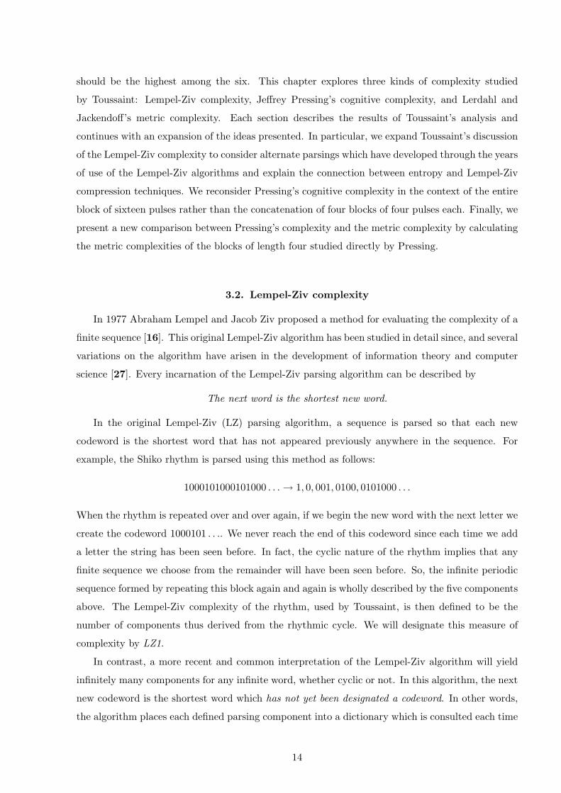
should be the highest among the six. This chapter explores three kinds of complexity studied

by Toussaint: Lempel-Ziv complexity, Jeffrey Pressing’s cognitive complexity, and Lerdahl and

Jackendoff’s metric complexity. Each section describes the results of Toussaint’s analysis and

continues with an expansion of the ideas presented. In particular, we expand Toussaint’s discussion

of the Lempel-Ziv complexity to consider alternate parsings which have developed through the years

of use of the Lempel-Ziv algorithms and explain the connection between entropy and Lempel-Ziv

compression techniques. We reconsider Pressing’s cognitive complexity in the context of the entire

block of sixteen pulses rather than the concatenation of four blocks of four pulses each. Finally, we

present a new comparison between Pressing’s complexity and the metric complexity by calculating

the metric complexities of the blocks of length four studied directly by Pressing.

3.2. Lempel-Ziv complexity

In 1977 Abraham Lempel and Jacob Ziv proposed a method for evaluating the complexity of a

finite sequence [16]. This original Lempel-Ziv algorithm has been studied in detail since, and several

variations on the algorithm have arisen in the development of information theory and computer

science [27]. Every incarnation of the Lempel-Ziv parsing algorithm can be described by

The next word is the shortest new word.

In the original Lempel-Ziv (LZ) parsing algorithm, a sequence is parsed so that each new

codeword is the shortest word that has not appeared previously anywhere in the sequence. For

example, the Shiko rhythm is parsed using this method as follows:

1000101000101000 . . . → 1, 0, 001, 0100, 0101000 . . .

When the rhythm is repeated over and over again, if we begin the new word with the next letter we

create the codeword 1000101 . . .. We never reach the end of this codeword since each time we add

a letter the string has been seen before. In fact, the cyclic nature of the rhythm implies that any

finite sequence we choose from the remainder will have been seen before. So, the infinite periodic

sequence formed by repeating this block again and again is wholly described by the five components

above. The Lempel-Ziv complexity of the rhythm, used by Toussaint, is then defined to be the

number of components thus derived from the rhythmic cycle. We will designate this measure of

complexity by LZ1.

In contrast, a more recent and common interpretation of the Lempel-Ziv algorithm will yield

infinitely many components for any infinite word, whether cyclic or not. In this algorithm, the next

new codeword is the shortest word which has not yet been designated a codeword. In other words,

the algorithm places each defined parsing component into a dictionary which is consulted each time

14

LZ1 LZ2Shiko 5 8Son 6 8

Soukous 6 8Rumba 6 7

Bossa-Nova 5 8Gahu 5 8

Table 3.2. The Lempel-Ziv complexity measures of the six Clave rhythms

the next component is sought. For example, the new parsing of the Shiko rhythm is

10001010001010001000101000101000 . . . → 1, 0, 00, 10, 100, 01, 010, 001, 000, 101, 0001, 0100, . . . .

Analogously to the LZ1 complexity, we could define the LZ2 complexity of the rhythms as the

number of codewords into which the rhythm might be parsed in this way. Table 3.2 gives both

the LZ1 complexity calculated by Toussaint and the LZ2 complexity. According to both of the

measures, the six rhythms are all of approximately the same complexity.

The LZ2 parsing is common in the hunt for better and faster electrical communication and

computer coding. The usefulness of the technique lies in the connection between the LZ2 parsing

of a typical sequence output by an ergodic stationary process and the ergodic-theoretic entropy

of that process. (In fact, all of the results we give in this section apply also to the LZ1 parsing

technique. In the discussion following, we will use the term ”Lempel-Ziv” to refer jointly to LZ1

and LZ2.) Either Lempel-Ziv parsing acting on an ergodic process compresses the infinite process

to its entropy in the limit.

First, notice that each codeword is either a single element of the alphabet {0, 1} or is of the form

ω(j)a, where ω(j) represents a prefix seen earlier in the sequence and a represents a single element

of the alphabet {0, 1}. The Lempel-Ziv n-code Dn then encodes the location of the prefix ω(j) and

its last element a. In the LZ1 parsing, the location of ω(j) is the location where it is first observed

in the sequence so far. In the LZ2 parsing, the location of ω(j) is its position in the dictionary of

codewords being created. In the notation of [?], the LZ2 parsing of 011000101001111010. . . would

be as follows:

0, 1, 10, 00, 101, 001, 11, 1010, . . .

and the LZ2 compression is

(000, 0)(000, 1)(010, 0)(001, 0)(011, 1)(100, 1)(010, 1)(101, 0)

The first codeword, namely 0, has no prefix. So the location of the prefix (000) is encoded base

2 followed by the digit 0 which is added to the end. The prefix of the fifth codeword, 101, is 10

– the third codeword. So the location of the prefix is recorded base 2 (11) and the digit added

15

to the end (1) is also recorded. In this small example, the length of the “compression” is actually

greater than the length of the sequence. However, as the length of the original sequence increases,

the compression becomes increasingly efficient. In fact, the compression tends toward the entropy

as the length tends toward infinity, as we will see below.

If CN is the number of codewords in the parsing of a sequence of length N , then we need

log2 CN bits to describe the location of the prefix and 1 bit to describe the last bit. So for each

ω(i) we need log2 CN + 1 bits to encode ω(i) in the Lempel-Ziv code. In other words, DN (xN1 ) has

length CN (log2 CN + 1) bits. Theorem 3.2.1, in its original form due to Lempel and Ziv and later

proved by Ornstein and Weiss, states that for very large N , the Lempel-Ziv code length approaches

the entropy of the system. The proof and discussion which follow can all be found in [27].

Theorem 3.2.1. If µ is a stationary ergodic process with entropy h, then

(3.1) limN→∞

(CN (lnCN + 1))/N = h a.e..

One argument for the truth of Theorem 3.2.1 is based on the entropy equipartition prop-

erty, a consequence of the Shannon-McMillan-Breiman Theorem of ergodic theory. Denote αnm =∨n

k=m T−kα, where∨

denotes the least common refinement as found in [19].

Definition 3.2.1. The gain in information when we learn to which element of a partition α

the point x belongs is defined to be

Iα(x) = − log2 µ(α(x)) = −∑A∈α

log2 µ(A)χA(x).

Then Iαn−10

(x) = Iα∨

T−1α∨

...∨

T−n+1α(x) is the amount of information gained when we learn to

which elements of a partition α the elements x, T−1x, T−2x, etc. belong.

Theorem 3.2.2. (Shannon-McMillan-Breiman) Let T : X → X be an ergodic measure-preserving

transformation on (X,B, µ) and α a finite or countable measurable partition of X with H(α) =

−∑∞

i=1 µ(Ai) log2 µ(Ai) < ∞. Then

Iαn−10

(x)

n→ h a.e. as n →∞.

The entropy equipartition property, also called the asymptotic equipartition property (AEP), in

its simplest form [1] tells us that “almost everything is almost equally probable.” In its precise

form, it states:

Theorem 3.2.3. (Entropy equipartition property) Let T : X → X be ergodic and α =

{A1, A2, ...} a finite or countable measurable partition of X with H(α) = −∑∞

i=1 µ(Ai) log2 µ(Ai) <

∞. Given ε > 0 there is an n0 such that for n ≥ n0 the elements of αn0 can be divided into “good”

16

and “bad” classes (γ and β, respectively) such that:

(i) µ⋃

B∈β B < ε, and

(ii) for each G ∈ γ,

2−n(h+ε) < µ(G) < 2−n(h−ε).

Proof. Since Iαn−10

/n → h a.e., Iαn−10

/n → h in measure: for each ε > 0 there is an n0 such that if

n ≥ n0 then

µ{x : |(Iαn−10

/n)− h| ≥ ε} < ε.

But Iαn−10

must be constant on each cell of αn−10 by definition. So, we let γ be those elements of

αn−10 for which |Iαn−1

0/n− h| < ε and let β be everything else. ♦

The summary “almost everything is almost equally probable” is justified as follows. Choosing

a sequence εm → 0, it is clear that for large n, µ(γ) ≈ 1 and µ(β) ≈ 0. Then on average each G ∈ γ

(namely, each element of αn−10 with positive measure) will have measure approximately equal to

2−nh. So, there will be approximately 2nh such elements G.

Now let us apply this to the Lempel-Ziv code. The average length of the CN codewords is

n ≈ N

CN.

The entropy equipartition property then implies that for very large N there are approximately

2(N/CN )h “typical” blocks of length n ≈ N/CN . So,

CN ≈ 2(N/CN )h.

Taking logarithms of both sides, we get

CN log2 CN

N≈ h

for very large N . This outline of a proof gives us an idea why the Lempel-Ziv theorem holds with

convergence in measure.

Another argument for the Lempel-Ziv convergence theorem uses the first return time formula

studied first by Wyner and Ziv and later by Ornstein and Weiss. If x = x1x2x3... ∈ A∞1 , we define

the first return time of xn1 as

Rn(x) = min{m ≥ 1 : xm+nm+1 = xn

1}.

Theorem 3.2.4. For any ergodic process µ with entropy h,

(3.2) limn→∞

log2 Rn(x)n

= h a.e.

17

The proof of the Ornstein-Weiss first-return time theorem is quite long and involved. It can be

done in three parts. Initially, the upper and lower limits are defined:

r(x) = lim supn→∞

log2 Rn(x)n

and

r(x) = lim infn→∞

log2 Rn(x)n

.

These limits are shown to be a.e.-equal to constants r and r, respectively, with r ≤ r, clearly. Wyner

and Ziv proved that r ≤ h by showing that for ε > 0, µ{x : Rn(x) > 2n(h+ε)} → 0 as n → ∞,

implying that for every ε and for most x, there exists an n0 such that for n > n0,

Rn(x) ≤ 2n(h+ε), and hencelog2 Rn(x)

n− ε ≤ h.

The other inequality, namely r ≥ h, as proved by Ornstein and Weiss, is a proof by contradiction:

if it is not true one can build a code that compresses to less than the entropy.

Since the shift transformation is ergodic, we can consider one of the CN “typical” codewords

as discussed in the last argument. Such an average codeword will have length

n ≈ N

CN.

By Kac’ Theorem, in an ergodic system the expected recurrence time of a subset A ⊆ X is 1/µ(A).

Because each cylinder corresponding to a “typical” codeword has about the same measure,

Rn ≈1

µ(CN )≈ CN .

Thus by Theorem 3.2.4, almost surely

(3.3)CN log2 CN

N=

log2 CN

N/CN≈ log2 Rn

n→ h.

We demonstrate an application of these theorems by verifying that any periodic process, such

as one arising from repeating a single Clave pattern over and over, has entropy 0. If we consider

the LZ1 parsing of a periodic sequence having period p, then CN ≤ p + 1 for every N . So,

(CN (log2 CN + 1))/N ≤ (p + 1)(log2 (p + 1) + 1)N

→ 0 as N →∞.

Now consider a parsing of a cyclic sequence of period n using the second method. While we could

use Theorem 3.2.1 to show again that the entropy is zero, the argument is somewhat simpler from

Theorem 3.2.4. Again for a cyclic sequence of period p, for any n, Rn(x) = min{m ≥ 1 : xm+nm+1 =

xn1} ≤ p. So,

(3.4) (log2 Rn(x))/n ≤ p/n → 0 as n →∞.

18

These results agree with the intuitive definition of entropy given by Pierce: after we pass through

only one cycle, no other information is gained from any subsequent letter. Thus we confirm that

the entropy of a cyclic sequence such as one generated by one of the rhythms is zero.

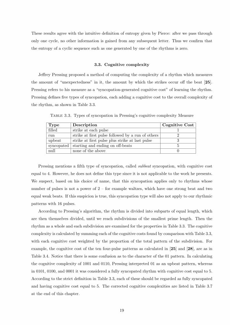
3.3. Cognitive complexity

Jeffrey Pressing proposed a method of computing the complexity of a rhythm which measures

the amount of “unexpectedness” in it, the amount by which the strikes occur off the beat [25].

Pressing refers to his measure as a “syncopation-generated cognitive cost” of learning the rhythm.

Pressing defines five types of syncopation, each adding a cognitive cost to the overall complexity of

the rhythm, as shown in Table 3.3.

Table 3.3. Types of syncopation in Pressing’s cognitive complexity Measure

Type Description Cognitive Costfilled strike at each pulse 1run strike at first pulse followed by a run of others 2upbeat strike at first pulse plus strike at last pulse 3syncopated starting and ending on off-beats 5null none of the above 0

Pressing mentions a fifth type of syncopation, called subbeat syncopation, with cognitive cost

equal to 4. However, he does not define this type since it is not applicable to the work he presents.

We suspect, based on his choice of name, that this syncopation applies only to rhythms whose

number of pulses is not a power of 2 – for example waltzes, which have one strong beat and two

equal weak beats. If this suspicion is true, this syncopation type will also not apply to our rhythmic

patterns with 16 pulses.

According to Pressing’s algorithm, the rhythm is divided into subparts of equal length, which

are then themselves divided, until we reach subdivisions of the smallest prime length. Then the

rhythm as a whole and each subdivision are examined for the properties in Table 3.3. The cognitive

complexity is calculated by summing each of the cognitive costs found by comparison with Table 3.3,

with each cognitive cost weighted by the proportion of the total pattern of the subdivision. For

example, the cognitive cost of the ten four-pulse patterns as calculated in [25] and [28], are as in

Table 3.4. Notice that there is some confusion as to the character of the 01 pattern. In calculating

the cognitive complexity of 1001 and 0110, Pressing interpreted 01 as an upbeat pattern, whereas

in 0101, 0100, and 0001 it was considered a fully syncopated rhythm with cognitive cost equal to 5.

According to the strict definition in Table 3.3, each of these should be regarded as fully syncopated

and having cognitive cost equal to 5. The corrected cognitive complexities are listed in Table 3.7

at the end of this chapter.

19

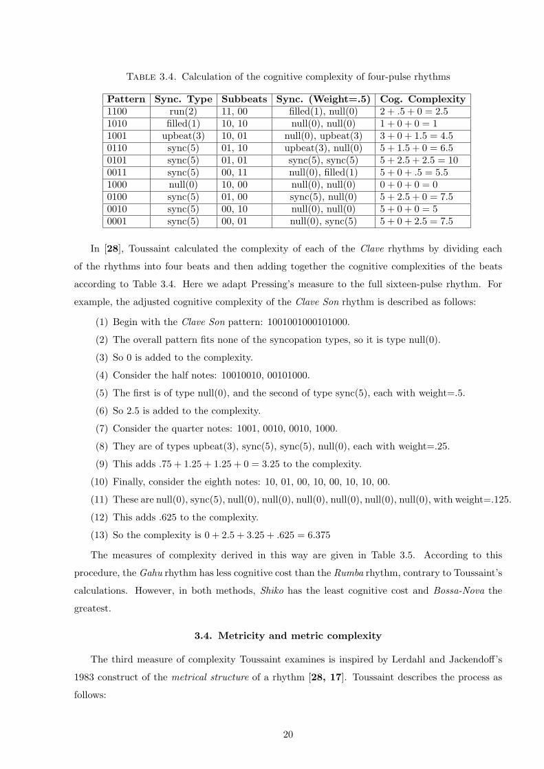
Table 3.4. Calculation of the cognitive complexity of four-pulse rhythms

Pattern Sync. Type Subbeats Sync. (Weight=.5) Cog. Complexity1100 run(2) 11, 00 filled(1), null(0) 2 + .5 + 0 = 2.51010 filled(1) 10, 10 null(0), null(0) 1 + 0 + 0 = 11001 upbeat(3) 10, 01 null(0), upbeat(3) 3 + 0 + 1.5 = 4.50110 sync(5) 01, 10 upbeat(3), null(0) 5 + 1.5 + 0 = 6.50101 sync(5) 01, 01 sync(5), sync(5) 5 + 2.5 + 2.5 = 100011 sync(5) 00, 11 null(0), filled(1) 5 + 0 + .5 = 5.51000 null(0) 10, 00 null(0), null(0) 0 + 0 + 0 = 00100 sync(5) 01, 00 sync(5), null(0) 5 + 2.5 + 0 = 7.50010 sync(5) 00, 10 null(0), null(0) 5 + 0 + 0 = 50001 sync(5) 00, 01 null(0), sync(5) 5 + 0 + 2.5 = 7.5

In [28], Toussaint calculated the complexity of each of the Clave rhythms by dividing each

of the rhythms into four beats and then adding together the cognitive complexities of the beats

according to Table 3.4. Here we adapt Pressing’s measure to the full sixteen-pulse rhythm. For

example, the adjusted cognitive complexity of the Clave Son rhythm is described as follows:

(1) Begin with the Clave Son pattern: 1001001000101000.

(2) The overall pattern fits none of the syncopation types, so it is type null(0).

(3) So 0 is added to the complexity.

(4) Consider the half notes: 10010010, 00101000.

(5) The first is of type null(0), and the second of type sync(5), each with weight=.5.

(6) So 2.5 is added to the complexity.

(7) Consider the quarter notes: 1001, 0010, 0010, 1000.

(8) They are of types upbeat(3), sync(5), sync(5), null(0), each with weight=.25.

(9) This adds .75 + 1.25 + 1.25 + 0 = 3.25 to the complexity.

(10) Finally, consider the eighth notes: 10, 01, 00, 10, 00, 10, 10, 00.

(11) These are null(0), sync(5), null(0), null(0), null(0), null(0), null(0), null(0), with weight=.125.

(12) This adds .625 to the complexity.

(13) So the complexity is 0 + 2.5 + 3.25 + .625 = 6.375

The measures of complexity derived in this way are given in Table 3.5. According to this

procedure, the Gahu rhythm has less cognitive cost than the Rumba rhythm, contrary to Toussaint’s

calculations. However, in both methods, Shiko has the least cognitive cost and Bossa-Nova the

greatest.

3.4. Metricity and metric complexity

The third measure of complexity Toussaint examines is inspired by Lerdahl and Jackendoff’s

1983 construct of the metrical structure of a rhythm [28, 17]. Toussaint describes the process as

follows:

20

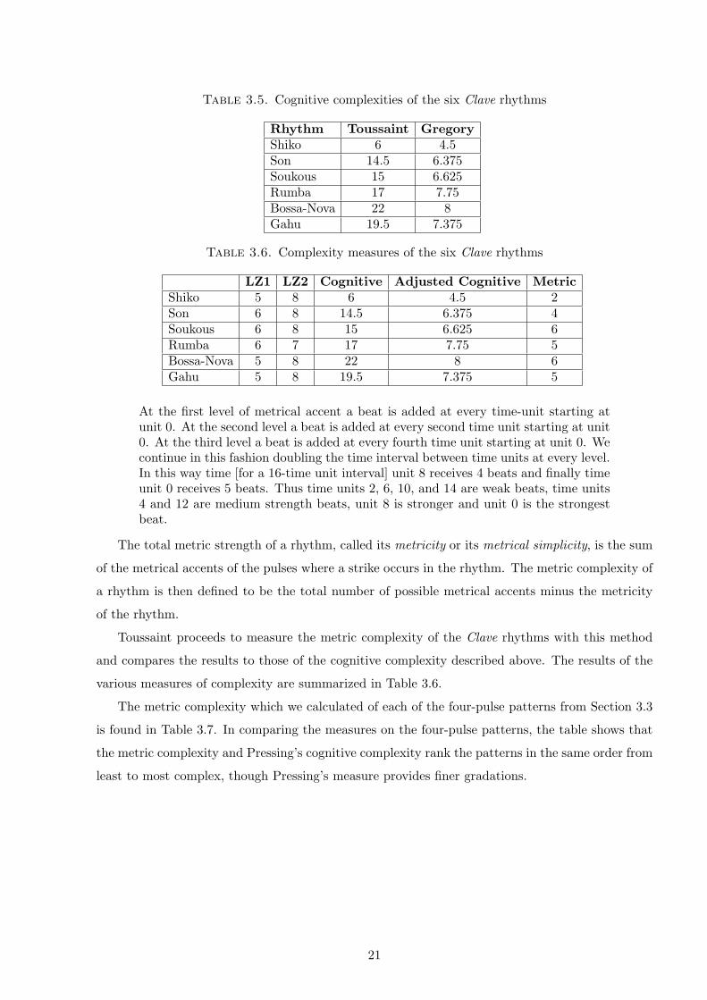
Table 3.5. Cognitive complexities of the six Clave rhythms

Rhythm Toussaint GregoryShiko 6 4.5Son 14.5 6.375Soukous 15 6.625Rumba 17 7.75Bossa-Nova 22 8Gahu 19.5 7.375

Table 3.6. Complexity measures of the six Clave rhythms

LZ1 LZ2 Cognitive Adjusted Cognitive MetricShiko 5 8 6 4.5 2Son 6 8 14.5 6.375 4Soukous 6 8 15 6.625 6Rumba 6 7 17 7.75 5Bossa-Nova 5 8 22 8 6Gahu 5 8 19.5 7.375 5

At the first level of metrical accent a beat is added at every time-unit starting atunit 0. At the second level a beat is added at every second time unit starting at unit0. At the third level a beat is added at every fourth time unit starting at unit 0. Wecontinue in this fashion doubling the time interval between time units at every level.In this way time [for a 16-time unit interval] unit 8 receives 4 beats and finally timeunit 0 receives 5 beats. Thus time units 2, 6, 10, and 14 are weak beats, time units4 and 12 are medium strength beats, unit 8 is stronger and unit 0 is the strongestbeat.

The total metric strength of a rhythm, called its metricity or its metrical simplicity, is the sum

of the metrical accents of the pulses where a strike occurs in the rhythm. The metric complexity of

a rhythm is then defined to be the total number of possible metrical accents minus the metricity

of the rhythm.

Toussaint proceeds to measure the metric complexity of the Clave rhythms with this method

and compares the results to those of the cognitive complexity described above. The results of the

various measures of complexity are summarized in Table 3.6.

The metric complexity which we calculated of each of the four-pulse patterns from Section 3.3

is found in Table 3.7. In comparing the measures on the four-pulse patterns, the table shows that

the metric complexity and Pressing’s cognitive complexity rank the patterns in the same order from

least to most complex, though Pressing’s measure provides finer gradations.

21

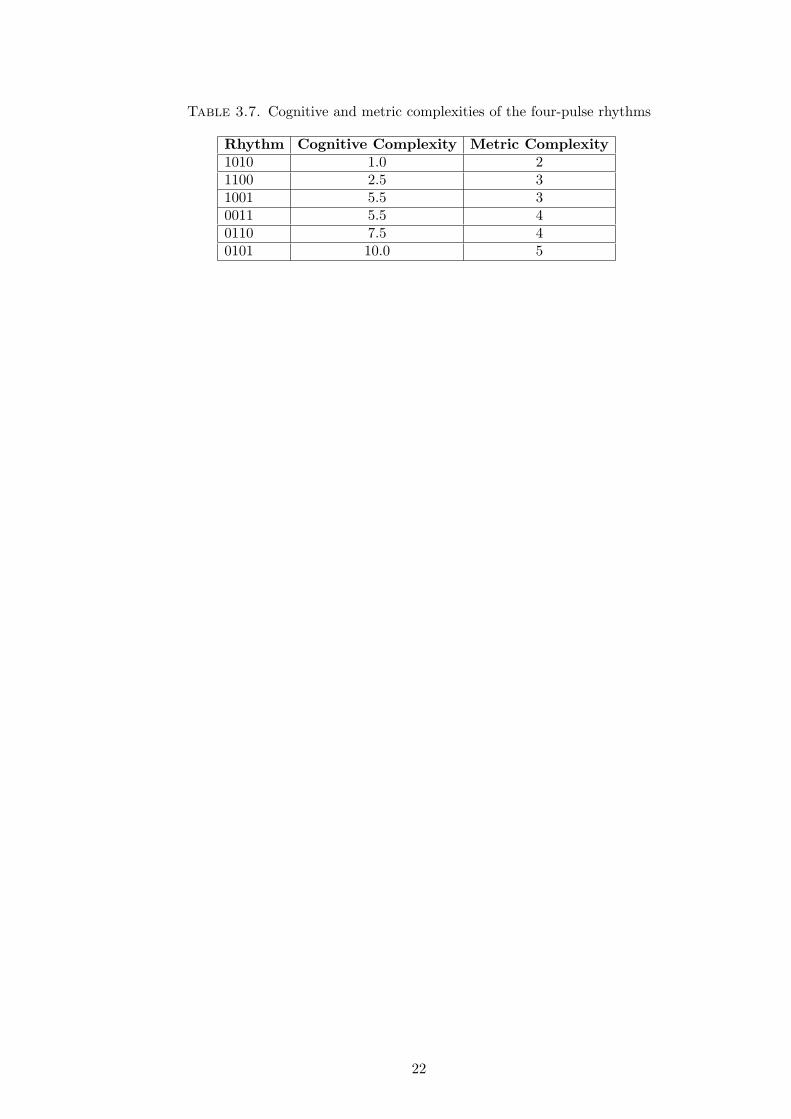
Table 3.7. Cognitive and metric complexities of the four-pulse rhythms

Rhythm Cognitive Complexity Metric Complexity1010 1.0 21100 2.5 31001 5.5 30011 5.5 40110 7.5 40101 10.0 5

22

CHAPTER 4

The traditional Nzakara harpists

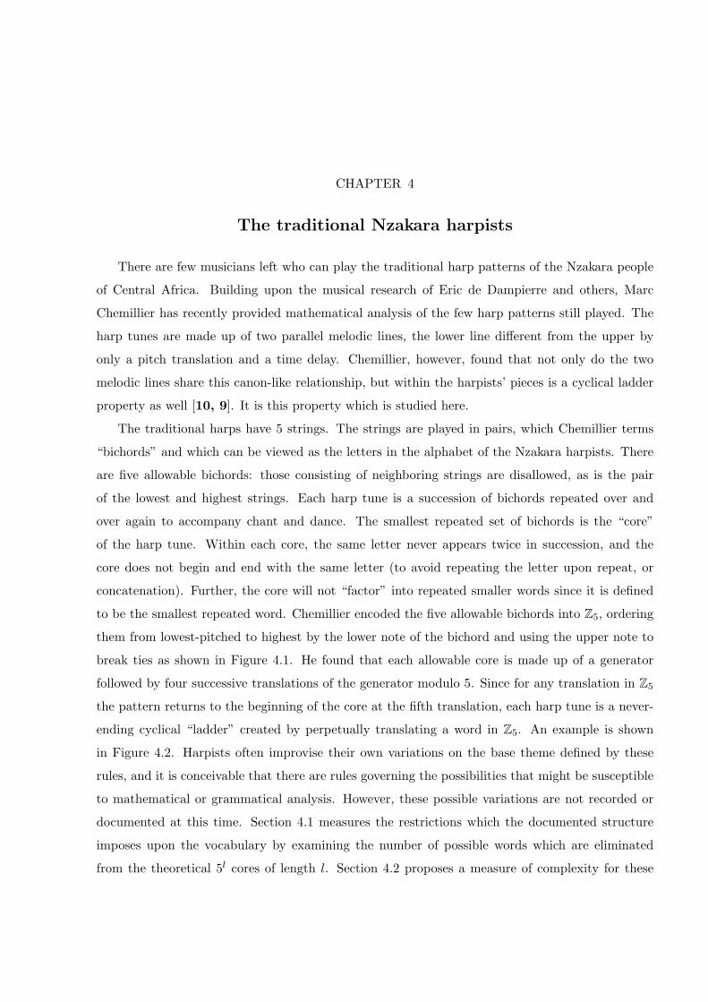
There are few musicians left who can play the traditional harp patterns of the Nzakara people

of Central Africa. Building upon the musical research of Eric de Dampierre and others, Marc

Chemillier has recently provided mathematical analysis of the few harp patterns still played. The

harp tunes are made up of two parallel melodic lines, the lower line different from the upper by

only a pitch translation and a time delay. Chemillier, however, found that not only do the two

melodic lines share this canon-like relationship, but within the harpists’ pieces is a cyclical ladder

property as well [10, 9]. It is this property which is studied here.

The traditional harps have 5 strings. The strings are played in pairs, which Chemillier terms

“bichords” and which can be viewed as the letters in the alphabet of the Nzakara harpists. There

are five allowable bichords: those consisting of neighboring strings are disallowed, as is the pair

of the lowest and highest strings. Each harp tune is a succession of bichords repeated over and

over again to accompany chant and dance. The smallest repeated set of bichords is the “core”

of the harp tune. Within each core, the same letter never appears twice in succession, and the

core does not begin and end with the same letter (to avoid repeating the letter upon repeat, or

concatenation). Further, the core will not “factor” into repeated smaller words since it is defined

to be the smallest repeated word. Chemillier encoded the five allowable bichords into Z5, ordering

them from lowest-pitched to highest by the lower note of the bichord and using the upper note to

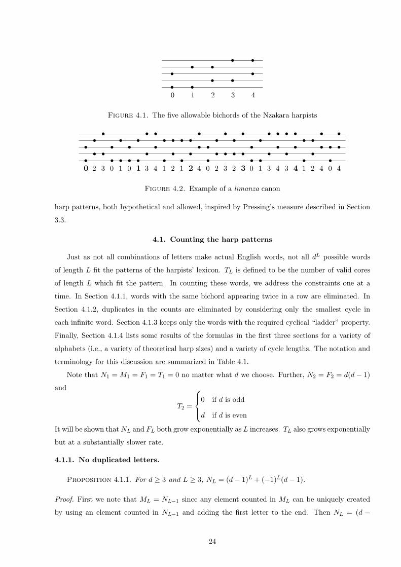
break ties as shown in Figure 4.1. He found that each allowable core is made up of a generator

followed by four successive translations of the generator modulo 5. Since for any translation in Z5

the pattern returns to the beginning of the core at the fifth translation, each harp tune is a never-

ending cyclical “ladder” created by perpetually translating a word in Z5. An example is shown

in Figure 4.2. Harpists often improvise their own variations on the base theme defined by these

rules, and it is conceivable that there are rules governing the possibilities that might be susceptible

to mathematical or grammatical analysis. However, these possible variations are not recorded or

documented at this time. Section 4.1 measures the restrictions which the documented structure

imposes upon the vocabulary by examining the number of possible words which are eliminated

from the theoretical 5l cores of length l. Section 4.2 proposes a measure of complexity for these

ss ss ss s

s ss

0 1 2 3 4

Figure 4.1. The five allowable bichords of the Nzakara harpists

s s s s s s s s s s s s s s s s s s s s s s s s s s s s s ss s s s s s s s s s s s s s s s s s s s s s s s s s s s s s

0 2 3 0 1 0 1 3 4 1 2 1 2 4 0 2 3 2 3 0 1 3 4 3 4 1 2 4 0 4

Figure 4.2. Example of a limanza canon

harp patterns, both hypothetical and allowed, inspired by Pressing’s measure described in Section

3.3.

4.1. Counting the harp patterns

Just as not all combinations of letters make actual English words, not all dL possible words

of length L fit the patterns of the harpists’ lexicon. TL is defined to be the number of valid cores

of length L which fit the pattern. In counting these words, we address the constraints one at a

time. In Section 4.1.1, words with the same bichord appearing twice in a row are eliminated. In

Section 4.1.2, duplicates in the counts are eliminated by considering only the smallest cycle in

each infinite word. Section 4.1.3 keeps only the words with the required cyclical “ladder” property.

Finally, Section 4.1.4 lists some results of the formulas in the first three sections for a variety of

alphabets (i.e., a variety of theoretical harp sizes) and a variety of cycle lengths. The notation and

terminology for this discussion are summarized in Table 4.1.

Note that N1 = M1 = F1 = T1 = 0 no matter what d we choose. Further, N2 = F2 = d(d− 1)

and

T2 =

0 if d is odd

d if d is even

It will be shown that NL and FL both grow exponentially as L increases. TL also grows exponentially

but at a substantially slower rate.

4.1.1. No duplicated letters.

Proposition 4.1.1. For d ≥ 3 and L ≥ 3, NL = (d− 1)L + (−1)L(d− 1).

Proof. First we note that ML = NL−1 since any element counted in ML can be uniquely created

by using an element counted in NL−1 and adding the first letter to the end. Then NL = (d −

24

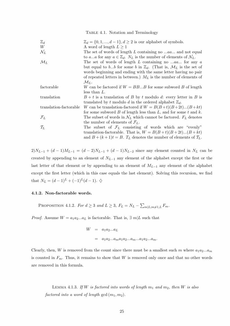
Table 4.1. Notation and Terminology

Zd Zd = {0, 1, ..., d− 1}, d ≥ 2 is our alphabet of symbols.W A word of length L ≥ 1NL The set of words of length L containing no ...aa... and not equal

to a...a for any a ∈ Zd. NL is the number of elements of NL.ML The set of words of length L containing no ...aa... for any a

but equal to b...b for some b in Zd. (That is, ML is the set ofwords beginning and ending with the same letter having no pairof repeated letters in between.) ML is the number of elements ofML.

factorable W can be factored if W = BB...B for some subword B of lengthless than L.

translation B + t is a translation of B by t modulo d: every letter in B istranslated by t modulo d in the ordered alphabet Zd.

translation-factorable W can be translation-factored if W = B(B+t)(B+2t)...(B+kt)for some subword B of length less than L, and for some t and k.

FL The subset of words in NL which cannot be factored. FL denotesthe number of elements of FL.

TL The subset of FL consisting of words which are “evenly”translation-factorable. That is, W = B(B + t)(B +2t)...(B + kt)and B + (k + 1)t = B. TL denotes the number of elements of TL.

2)NL−1 + (d − 1)ML−1 = (d − 2)NL−1 + (d − 1)NL−2 since any element counted in NL can be

created by appending to an element of NL−1 any element of the alphabet except the first or the

last letter of that element or by appending to an element of ML−1 any element of the alphabet

except the first letter (which in this case equals the last element). Solving this recursion, we find

that NL = (d− 1)L + (−1)L(d− 1). ♦

4.1.2. Non-factorable words.

Proposition 4.1.2. For d ≥ 3 and L ≥ 3, FL = NL −∑

m|L;m6=1,L Fm.

Proof. Assume W = a1a2...aL is factorable. That is, ∃ m|L such that

W = a1a2...aL

= a1a2...ama1a2...am...a1a2...am.

Clearly, then, W is removed from the count since there must be a smallest such m where a1a2...am

is counted in Fm. Thus, it remains to show that W is removed only once and that no other words

are removed in this formula.

Lemma 4.1.3. If W is factored into words of length m1 and m2, then W is also

factored into a word of length gcd (m1,m2).

25

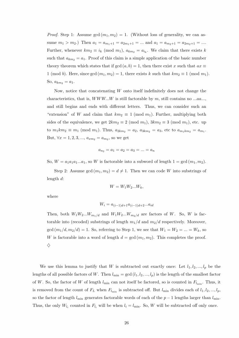
Proof. Step 1: Assume gcd (m1,m2) = 1. (Without loss of generality, we can as-

sume m1 > m2.) Then a1 = am1+1 = a2m1+1 = ... and a1 = am2+1 = a2m2+1 = ....

Further, whenever km2 ≡ ik (mod m1), akm2 = aik . We claim that there exists k

such that akm2 = a1. Proof of this claim is a simple application of the basic number

theory theorem which states that if gcd (a, b) = 1, then there exist x such that ax ≡

1 (mod b). Here, since gcd (m1,m2) = 1, there exists k such that km2 ≡ 1 (mod m1).

So, akm2 = a1.

Now, notice that concatenating W onto itself indefinitely does not change the

characteristics, that is, WWW...W is still factorable by m, still contains no ...aa...,

and still begins and ends with different letters. Thus, we can consider such an

“extension” of W and claim that km2 ≡ 1 (mod m1). Further, multiplying both

sides of the equivalence, we get 2km2 ≡ 2 (mod m1), 3km2 ≡ 3 (mod m1), etc. up

to m1km2 ≡ m1 (mod m1). Thus, a2km2 = a2, a3km2 = a3, etc to am1km2 = am1 .

But, ∀x = 1, 2, 3, ..., axm2 = am2 , so we get

an2 = a1 = a2 = a3 = ... = an

So, W = a1a1a1...a1, so W is factorable into a subword of length 1 = gcd (m1,m2).

Step 2: Assume gcd (m1,m2) = d 6= 1. Then we can code W into substrings of

length d:

W = W1W2...Wk,

where

Wi = a(i−1)d+1a(i−1)d+2...aid

Then, both W1W2...Wm1/d and W1W2...Wm2/d are factors of W . So, W is fac-

torable into (recoded) substrings of length m1/d and m2/d respectively. Moreover,

gcd (m1/d,m2/d) = 1. So, referring to Step 1, we see that W1 = W2 = ... = Wk, so

W is factorable into a word of length d = gcd (m1,m2). This completes the proof.

♦

We use this lemma to justify that W is subtracted out exactly once: Let l1, l2, ..., lp be the

lengths of all possible factors of W . Then lmin = gcd (l1, l2, ..., lp) is the length of the smallest factor

of W . So, the factor of W of length lmin can not itself be factored, so is counted in Flmin. Thus, it

is removed from the count of FL when Flminis subtracted off. But lmin divides each of l1, l2, ..., lp,

so the factor of length lmin generates factorable words of each of the p− 1 lengths larger than lmin.

Thus, the only Wli counted in Fli will be when li = lmin. So, W will be subtracted off only once.

26

Further,∑

m|L;m6=1,L Fm is the total number of non-further-factorable factor-candidates for a

word W of length L. Thus, each of the words in this count generates a unique factorable word of

length L, so only factorable words are removed from the count NL. ♦

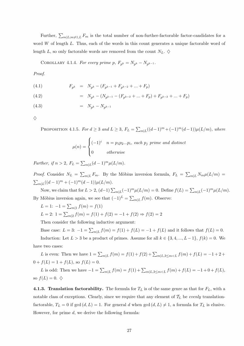
Corollary 4.1.4. For every prime p, Fpk = Npk −Npk−1.

Proof.

Fpk = Npk − (Fpk−1 + Fpk−2 + ... + Fp)(4.1)

= Npk − (Npk−1 − (Fpk−2 + ... + Fp) + Fpk−2 + ... + Fp)(4.2)

= Npk −Npk−1(4.3)

♦

Proposition 4.1.5. For d ≥ 3 and L ≥ 3, FL =∑

m|L((d−1)m +(−1)m(d−1))µ(L/m), where

µ(n) =

(−1)i n = p1p2...pi, each pj prime and distinct

0 otherwise

Further, if n > 2, FL =∑

m|L(d− 1)mµ(L/m).

Proof. Consider NL =∑

m|L Fm. By the Mobius inversion formula, FL =∑

m|L Nmµ(L/m) =∑m|L((d− 1)m + (−1)m(d− 1))µ(L/m).

Now, we claim that for L > 2, (d−1)∑

m|L(−1)mµ(L/m) = 0. Define f(L) =∑

m|L(−1)mµ(L/m).

By Mobius inversion again, we see that (−1)L =∑

m|L f(m). Observe:

L = 1: −1 =∑

m|1 f(m) = f(1)

L = 2: 1 =∑

m|2 f(m) = f(1) + f(2) = −1 + f(2) ⇒ f(2) = 2

Then consider the following inductive argument:

Base case: L = 3: −1 =∑

m|L f(m) = f(1) + f(L) = −1 + f(L) and it follows that f(L) = 0.

Induction: Let L > 3 be a product of primes. Assume for all k ∈ {3, 4, ..., L− 1}, f(k) = 0. We

have two cases:

L is even: Then we have 1 =∑

m|L f(m) = f(1)+ f(2)+∑

m|L,3≤m<L f(m)+ f(L) = −1+2+

0 + f(L) = 1 + f(L), so f(L) = 0.

L is odd: Then we have −1 =∑

m|L f(m) = f(1)+∑

m|L,3≤m<L f(m)+ f(L) = −1+0+ f(L),

so f(L) = 0. ♦

4.1.3. Translation factorability. The formula for TL is of the same genre as that for FL, with a

notable class of exceptions. Clearly, since we require that any element of TL be evenly translation-

factorable, TL = 0 if gcd (d, L) = 1. For general d when gcd (d, L) 6= 1, a formula for TL is elusive.

However, for prime d, we derive the following formula:

27

Theorem 4.1.6. For prime d and L a multiple of d, TL = (d− 2)NL/d +(d− 1)ML/d−∑

Tk·d,

where the sum is over all k, 1 ≤ k < L/d; k|(L/d); and d · k is neither a divisor of, equal to, nor a

multiple of L/d.

Proof. The proof is in the derivation. Assume W is an evenly translation-factorable word of length

L whose letters are from Zd and which is not factorable. So, we can write W = a1a2...an(a1+t)(a2+

t)...(an + t)...(a1 + mt)(a2 + mt)...(an + mt) for some n and m. Then we know a1 = a1 + (m + 1)t

since W is evenly translation-factorable. Further, since W is not factorable, a1 6= a1 + pt for each

p ≤ m. So, since d is prime, a1, a1 + t, ...a1 + mt must be in one-to-one correspondence with the

elements of Zd. So, n = L/d and m = d− 1. So, any element of TL can be generated by an element

of either NL/d or of ML/d with some translation t. When we consider a generating element that

comes from NL/d, t cannot equal either 0 or aL/d − a1 since the former would lead to a factorable

W and the latter would lead to the appearance of a repeated letter in W . So, there are (d−2)NL/d

possible candidates for TL generated by elements of NL/d. Moreover, it is easy to see that no two of

these candidates are the same since either they will differ in the first L/d letters or in the L/d+1th

letter. When we consider a generating element of ML/d, t = 0 would lead to both factorability

and a repeated letter in the word W . So in this case, t 6= 0 is the only restriction on t. Thus

there are (d− 1)ML/d possible candidates for TL generated by elements of ML/d. Again, it is easy

to see that no two of these candidates is the same for the same reason as above. Further, each

candidate generated by ML/d is different from each candidate generated by NL/d: consider the

first and L/dth letters of two such candidates. If the first letter is the same, then the L/dth letters

must be different, by definition of NL/d and ML/d.

Each of these candidates satisfies the translation-factorability characteristic of elements of TL by

construction. Each candidate also satisfies the criterion that no letter is found twice in succession.

Further, candidates constructed in this manner do not factor into subwords of length L/d (by

construction), of length equal to any multiple of L/d (since this would imply a1 = a1 + pt for some

p < d), nor by length which divides L/d (since this would imply factorability into words of length

L/d). However, some of these candidates might factor into subwords of some other length which

divides L.

In order to count the number of candidates which factor into subwords of some other length,

we introduce the following lemma:

Lemma 4.1.7. If W of length L is translation-factorable by subwords of length

m1 and m2, m1 < m2 < L, then W is translation-factorable by a subword of length

m3 = m2 −m1.

28

Proof. Let s denote the translation associated with the subword of length m1 and

let t be that associated with m2.

Then, by definition, if we start at any ak for k = 1, 2, ..., L − m1, shifting m1

units to the right is equivalent to adding s to ak: ak+m1 = ak + s. Similarly, for

k = 1, 2, ..., L − m2 shifting m2 units to the right is equivalent to adding t to ak.

Further, observe that for k = m1 +1, ..., L, shifting m1 units to the left is equivalent

to subtracting s from ak; and for k = m2 + 1, ..., L, shifting m2 units to the left is

equivalent to subtracting t from ak.

Let k = 1, 2, ..., L−m2. (Note that m2 < L, m2 ≤ L/2 since otherwise W would

not be evenly translation-factorable. So L/2 ≤ L −m2 < L −m1, with the latter

inequality because m1 < m2.) Then consider ak+(m2−m1). This is ak shifted right

m2 units and then back left m1 units. So, we can write ak+(m2−m1) = ak + t− s, so

long as k + m2 > m1, which is clearly true since m2 > m1.

So, for all ak, k = 1, 2, ..., L−m2, ..., L−m2 + m2 −m1 = L−m1, we see that

we have a translation of a word of length m2 −m1 with translation by t − s. We

need now only explore the remaining m1 letters at the end of the word.

Consider, for k = L − m1 + 1, ..., L, ak−(m2−m1) = ak−m2+m1 . This is the

equivalent of shifting ak m2 units to the left and then m1 units to the right. So,

ak−(m2−m1) = ak−m2+m1 = ak − t + s. So, we again have a translation of a word

of length m2 −m1 with translation by t − s at the end of the word W . So, W is

translation-factorable by a word of length m2 −m1 with translation by t− s.

♦

Assume that a candidate W constructed as above is a concatenation of copies of a word W0

of length m for some m: W = (W0)L/m. Then we know m is not equal to, does not divide, and

is not a multiple of L/d. Consider the factorability of W into words of length m as a translation-

factorability of W into words of length m with translation by zero. Then by the lemma, we know

W must be translation-factorable into words of length |m−L/d| < L/d. We can apply the lemma

again to the smallest two of |m−L/d|, m, and L/d. Note that if we continue applying the lemma,

we find eventually that W must be translation-factorable into words of length gcdm,L/d. (The

repeated application of the lemma is a form of applying the Euclidean algorithm.) Let’s write

gcd m,L/d = mmin and denote the initial mmin letters of W as Wmin. Then there is some tmin

such that W0 = Wmin(Wmin + tmin)...(Wmin + (d− 1)tmin). Then each factorable word W counted

in the paragraphs above is associated with one and only one of the Td·mmin. Thus we arrive at

the summation term which subtracts out those candidates found in the complement of FL. This

completes the derivation and the proof. ♦

29

So, we can concatenate infinite copies any element of TL to create a harp pattern fitting Chemil-

lier’s bichord-translation requirements. Further, we can consider the shift action on a word of in-

finite length to be the mathematical equivalent of playing a succession of bichords on a Nzakara

harp. Under such considerations, observe that any periodic harp pattern will ultimately sound the

same no matter where we begin along its orbit under the shift action. So, ultimately, the number of

Nzakara harp pieces of a given length with a given alphabet is equal to the TL/L since any element

of TL will have a period of length L.

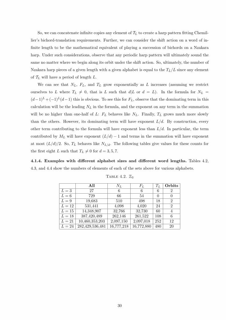
We can see that NL, FL, and TL grow exponentially as L increases (assuming we restrict

ourselves to L where TL 6= 0, that is L such that d|L or d = L). In the formula for NL =

(d−1)L +(−1)L(d−1) this is obvious. To see this for FL, observe that the dominating term in this

calculation will be the leading NL in the formula, and the exponent on any term in the summation

will be no higher than one-half of L: FL behaves like NL. Finally, TL grows much more slowly

than the others. However, its dominating term will have exponent L/d. By construction, every

other term contributing to the formula will have exponent less than L/d. In particular, the term

contributed by ML will have exponent (L/d) − 1 and terms in the summation will have exponent

at most (L/d)/2. So, TL behaves like NL/d. The following tables give values for these counts for

the first eight L such that TL 6= 0 for d = 3, 5, 7.

4.1.4. Examples with different alphabet sizes and different word lengths. Tables 4.2,

4.3, and 4.4 show the numbers of elements of each of the sets above for various alphabets.

Table 4.2. Z3

All NL FL TL OrbitsL = 3 27 6 6 6 2L = 6 729 66 54 0 0L = 9 19,683 510 498 18 2L = 12 531,441 4,098 4,020 24 2L = 15 14,348,907 32,766 32,730 60 4L = 18 387,420,489 262,146 261,522 108 6L = 21 10,460,353,203 2,097,150 2,097,018 252 12L = 24 282,429,536,481 16,777,218 16,772,880 480 20

30

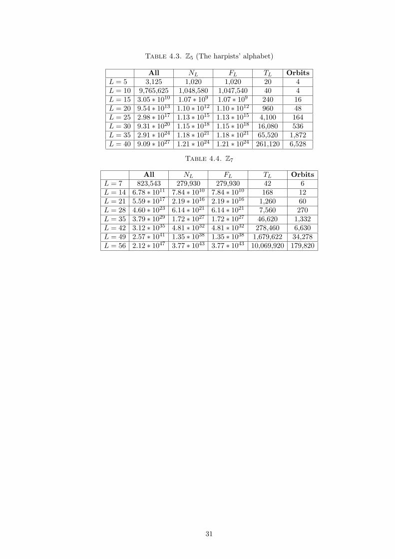
Table 4.3. Z5 (The harpists’ alphabet)

All NL FL TL OrbitsL = 5 3,125 1,020 1,020 20 4L = 10 9,765,625 1,048,580 1,047,540 40 4L = 15 3.05 ∗ 1010 1.07 ∗ 109 1.07 ∗ 109 240 16L = 20 9.54 ∗ 1013 1.10 ∗ 1012 1.10 ∗ 1012 960 48L = 25 2.98 ∗ 1017 1.13 ∗ 1015 1.13 ∗ 1015 4,100 164L = 30 9.31 ∗ 1020 1.15 ∗ 1018 1.15 ∗ 1018 16,080 536L = 35 2.91 ∗ 1024 1.18 ∗ 1021 1.18 ∗ 1021 65,520 1,872L = 40 9.09 ∗ 1027 1.21 ∗ 1024 1.21 ∗ 1024 261,120 6,528

Table 4.4. Z7

All NL FL TL OrbitsL = 7 823,543 279,930 279,930 42 6L = 14 6.78 ∗ 1011 7.84 ∗ 1010 7.84 ∗ 1010 168 12L = 21 5.59 ∗ 1017 2.19 ∗ 1016 2.19 ∗ 1016 1,260 60L = 28 4.60 ∗ 1023 6.14 ∗ 1021 6.14 ∗ 1021 7,560 270L = 35 3.79 ∗ 1029 1.72 ∗ 1027 1.72 ∗ 1027 46,620 1,332L = 42 3.12 ∗ 1035 4.81 ∗ 1032 4.81 ∗ 1032 278,460 6,630L = 49 2.57 ∗ 1041 1.35 ∗ 1038 1.35 ∗ 1038 1,679,622 34,278L = 56 2.12 ∗ 1047 3.77 ∗ 1043 3.77 ∗ 1043 10,069,920 179,820

31

ss ss ss s

s ss

0 1 2 3 4

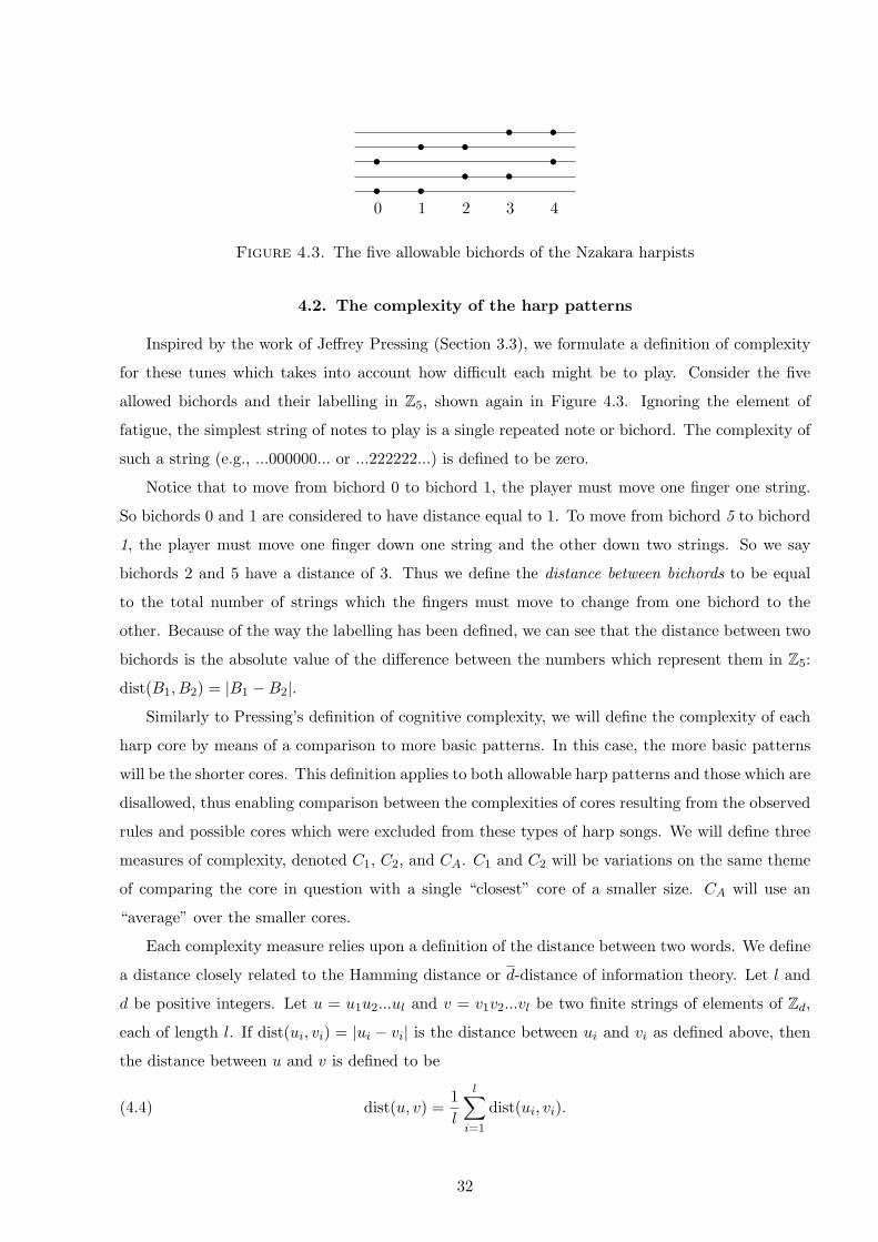
Figure 4.3. The five allowable bichords of the Nzakara harpists

4.2. The complexity of the harp patterns

Inspired by the work of Jeffrey Pressing (Section 3.3), we formulate a definition of complexity

for these tunes which takes into account how difficult each might be to play. Consider the five

allowed bichords and their labelling in Z5, shown again in Figure 4.3. Ignoring the element of

fatigue, the simplest string of notes to play is a single repeated note or bichord. The complexity of

such a string (e.g., ...000000... or ...222222...) is defined to be zero.

Notice that to move from bichord 0 to bichord 1, the player must move one finger one string.

So bichords 0 and 1 are considered to have distance equal to 1. To move from bichord 5 to bichord

1, the player must move one finger down one string and the other down two strings. So we say

bichords 2 and 5 have a distance of 3. Thus we define the distance between bichords to be equal

to the total number of strings which the fingers must move to change from one bichord to the

other. Because of the way the labelling has been defined, we can see that the distance between two

bichords is the absolute value of the difference between the numbers which represent them in Z5:

dist(B1, B2) = |B1 −B2|.

Similarly to Pressing’s definition of cognitive complexity, we will define the complexity of each

harp core by means of a comparison to more basic patterns. In this case, the more basic patterns

will be the shorter cores. This definition applies to both allowable harp patterns and those which are

disallowed, thus enabling comparison between the complexities of cores resulting from the observed

rules and possible cores which were excluded from these types of harp songs. We will define three

measures of complexity, denoted C1, C2, and CA. C1 and C2 will be variations on the same theme

of comparing the core in question with a single “closest” core of a smaller size. CA will use an

“average” over the smaller cores.

Each complexity measure relies upon a definition of the distance between two words. We define

a distance closely related to the Hamming distance or d-distance of information theory. Let l and

d be positive integers. Let u = u1u2...ul and v = v1v2...vl be two finite strings of elements of Zd,

each of length l. If dist(ui, vi) = |ui − vi| is the distance between ui and vi as defined above, then

the distance between u and v is defined to be

(4.4) dist(u, v) =1l

l∑i=1

dist(ui, vi).

32

In short, the distance between two finite words of the same length is the average distance between

their corresponding letters.

Since the cores used in the harp patterns are repeated over and over in a cyclical pattern,

there is a straightforward definition of the distance between two finite cores of different lengths.

Consider u and v of positive lengths s and t, respectively. Define u′ to be u concatenated upon

itself lcm(s, t)/s times to create a word of length lcm(s, t), and define v′ to be v concatenated to

itself lcm(s, t)/t times to create another word of length lcm(s, t). Then the distance between u and

v is defined to be the distance between u′ and v′.

We define the nearest-neighbor complexity of a core of length 2 as the minimum of the distances

to cores of length 1. Both the C1 and C2 complexities of cores of length 2 are defined this way.

For example, the complexity of the core 01 is 0.5, since its distance from 0 and 1 is equal to 0.5:

C1(01) = C2(01) = 0.5. Similarly, C1(03) = C2(03) = 1.5, demonstrating the more difficult task of

moving both fingers between the 0 bichord and the 3 bichord than between the nearby 0 and 1.

The nearest-neighbor complexity of a core of length longer than 2 takes into account all shorter

cores which are “close to” the core under consideration as well as their complexities. There are

many reasonable variations on this theme, two of which are discussed here. In the first version,

C1, finding a nearby neighbor is considered of more importance than the complexity of that nearby

neighbor: the set of words of minimum distance is found and then complexity is minimized within

that set. In the second version, C2, complexity and distance are minimized together by finding the

minimum of their product.

More precisely, given a word u of length k > 2, let Vi be the set of words of length i which have

the minimum distance to u for all i < k:

Vi = {v|v is of length i, dist(u, v) ≤ dist(u, w) for all words w of length i}.

If i = 1, then s1(u) = dist(u, v) for any v in V1. (Note that s1(u) is well-defined since every element

of Vi has the same distance to u.) For i > 1 we define

si(u) = min{dist(u, v) · C1(v)|v ∈ Vi}.

Then the C1 complexity of u is defined to be

C1(u) =k−1∑i=1

si(u)ωi

,

where ωi is a weighting term.

Some possible weighting variables ωi are i, 5i, 5i−1, or i!. We have chosen to use ωi = 5i−1.

Since we are working with an alphabet of size 5, the number of possible words of length i is given

by 5i. Thus with this choice of ωi, the weight on each sum term approximates the number of

33

choices among which we minimized. Furthermore, because of computing resource limitations, the

summations resulting in Table 4.5 are truncated at 5. (Note that the distance function is bounded

by 4, so as i increases, the weight variable we chose will quickly dominate and the contribution

from the i’th term becomes inconsequential.)

Our second version of the nearest-neighbor complexity of a core u of length k minimizes both

the distance and complexity of the comparison words with equal importance:

s1(u) = min{dist(u, v)|v is a word of length 1}

for i > 1, si(u) = min{dist(u, v) · C2(v)|v is a word of length i}

Then C2 is the weighted sum of the si’s, as before:

C2(u) =k−1∑i=1

si(u)ωi

.

The calculations in Table 4.5 use the same weighting variable as the first version and truncate the

summation term in the same location.

The final complexity measure in the table, the complexity over averages, is calculated using the

average of distance times complexity over all the smaller v. In other words,

(4.5) CA(u) =k−1∑i=1

mean(dist(u, vi) · CA(vi))

ωi,

where the arithmetic means are taken over all Vi with length i.

As we see in Table 4.5, the C2 complexity measure appears to do the best job of finding the

distance a player’s hands must travel to play any pattern of bichords. For example, a harpist’s

hands can never move more than 4 strings with each succeeding note, yielding a “tune” alternating

between bichords 0 and 4, or . . . 040404040 . . .. This tune does indeed have the largest C2 complexity

in the table, with a measure of 2. However, it has among the lowest complexities with averages.

In contrast, a harpist playing the “tune” . . . 00000000010000000001 . . . moves his hands very little,

and this pattern has the lowest nearest-neighbor complexity in the table (0.15), while it has the

highest complexities with averages (2.74).

One reason that CA seems to be a poor measure for hand movement is demonstrated by a

simple example. Consider a harpist playing a sequence of bichord 0 alternating with bichord 1.

This harpist’s hands move the same amount between each bichord no matter the number of total

strings on the harp (i.e., the size of the alphabet). Consequently, the complexity of 01 should

remain constant across alphabet sizes. However, as the size of the harp grows, CA(01) will also

grow as it is compared to words farther and farther away. In general, words far away from the

word in question with high complexity have at least as much influence as close words with near

34

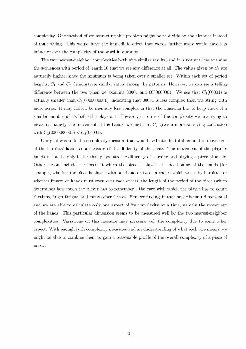
complexity. One method of counteracting this problem might be to divide by the distance instead

of multiplying. This would have the immediate effect that words further away would have less

influence over the complexity of the word in question.

The two nearest-neighbor complexities both give similar results, and it is not until we examine

the sequences with period of length 10 that we see any difference at all. The values given by C1 are

naturally higher, since the minimum is being taken over a smaller set. Within each set of period

lengths, C1 and C2 demonstrate similar ratios among the patterns. However, we can see a telling

difference between the two when we examine 00001 and 0000000001. We see that C1(00001) is

actually smaller than C1(0000000001), indicating that 00001 is less complex than the string with

more zeros. It may indeed be mentally less complex in that the musician has to keep track of a

smaller number of 0’s before he plays a 1. However, in terms of the complexity we are trying to

measure, namely the movement of the hands, we find that C2 gives a more satisfying conclusion

with C2(0000000001) < C2(00001).

Our goal was to find a complexity measure that would evaluate the total amount of movement

of the harpists’ hands as a measure of the difficulty of the piece. The movement of the player’s

hands is not the only factor that plays into the difficulty of learning and playing a piece of music.

Other factors include the speed at which the piece is played, the positioning of the hands (for

example, whether the piece is played with one hand or two – a choice which varies by harpist – or

whether fingers or hands must cross over each other), the length of the period of the piece (which

determines how much the player has to remember), the care with which the player has to count

rhythms, finger fatigue, and many other factors. Here we find again that music is multidimensional

and we are able to calculate only one aspect of its complexity at a time, namely the movement

of the hands. This particular dimension seems to be measured well by the two nearest-neighbor

complexities. Variations on this measure may measure well the complexity due to some other

aspect. With enough such complexity measures and an understanding of what each one means, we

might be able to combine them to gain a reasonable profile of the overall complexity of a piece of

music.

35

Table 4.5. The computed complexities of selected bichord patterns

Bichord pattern C1 C2 CA

. . . 01010101010101. . . 0.5 0.5 1.7

. . . 02020202020202. . . 1 1 1.6

. . . 03030303030303. . . 1.5 1.5 1.7

. . . 04040404040404. . . 2 2 2

. . . 010010010010010. . . 0.38 0.38 2.38

. . . 012012012012012. . . 0.75 0.75 2.03

. . . 013013013013013. . . 1.12 1.12 2.12

. . . 024024024024024. . . 1.48 1.48 2.29

. . . 000010000100001. . . 0.26 0.26 2.67

. . . 000020000200002. . . 0.48 0.48 2.62

. . . 012340123401234. . . ∗ 1.35 1.35 2.29

. . . 024130241302413. . . ∗ 1.35 1.35 2.29

. . . 031420314203142. . . ∗ 1.35 1.35 2.29

. . . 043210432104321. . . ∗ 1.35 1.35 2.29

. . . 021340213402134. . . ∗∗ 1.35 1.35 2.29

. . . 012310123101231. . . ∗∗ 0.91 0.91 2.12

. . . 023040230402304. . . ∗∗ 1.58 1.58 2.45

. . . 113231132311323. . . ∗∗ 0.91 0.91 1.95

. . . 034140341403414. . . ∗∗ 1.58 1.58 2.51

. . . 00000000010000000001. . . 0.54 0.15 2.74

. . . 01000100000100010000. . . 0.68 0.24 2.64

. . . 01341240230134124023. . . ∗ 3.00 1.35 2.06

. . . 02132430410213243041. . . ∗ 3.05 1.35 2.06

. . . 01403423120140342312. . . ∗ 3.00 1.35 2.06

. . . 01340243140134024314. . . ∗∗ 3.27 1.55 2.07

. . . 04241414420424141442. . . ∗∗ 3.25 1.53 1.85

. . . 01120440210112044021. . . ∗∗ 2.70 1.24 2.27∗ These patterns follow the grammatical rules of the harp tunes.

∗∗ These patterns were generated randomly for comparison.

36

CHAPTER 5

Conclusion

Every piece of music is an intricate balance of form, pitch, harmony, rhythm, and many intan-

gible aspects. The intricacy of these relationships and the impact they have on each other and on

the listener is impossible to measure completely. In this paper we have tried to understand some of

these individually by using ideas from information theory and mathematical linguistics. We have

set forth examples of how some of these tools may be used to examine the complexity (or richness

or difficulty or unexpectedness) of some of these aspects. Perhaps such techniques may allow a

musicologist to create a “complexity profile” of a type of music.

The concepts of entropy and complexity from information theory were used repeatedly through-

out this work. We have primarily used three general conceptions of complexity and entropy: as

a measure of the difficulty of learning or playing a sequence, as a measure of the amount of free-

dom and richness remaining within a defined structure, and as a degree of unexpectedness in a

sequence. The first definition was realized in rhythmic sequences in the cognitive complexity of the

Clave rhythms and in the various complexities we defined for the sequences of bichords played by

the Nzakara harpists. The second was examined in the discussion of Boulez’ ...explosante-fixe...,

Mozart’s Musikalisches Wurfelspiel, and the size of the Nzakara harpists’ potential vocabulary.

Finally, the third definition, that of the degree of unexpectedness in a sequence, was explored in

both the ...explosante-fixe... and Musikalisches Wurfelspiel discussions and in the sections on the

Lempel-Ziv and metric complexities of the Clave rhythms.

While these definitions of complexity and entropy are integrally related, there is yet no common

structure in which to interpret the results. Still some amount of comparison can be made. In the

case of the Clave rhythms, we found that both the metric complexity and the cognitive complexity

measures determined that the Bossa-Nova rhythm is the most difficult of the six while the Shiko is

the easiest, a result matching the experience of many students and musicians learning and playing

these rhythms. Further, given additional computing power, we would be able to compare the

complexities of the allowed bichord sequences of the Nzakara harp tunes to the disallowed of the

same order to seek some reason why perhaps the allowed tunes were preferred – are they easier to

play or are they more interesting than the others, for example.

We have gathered here a set of tools to study mathematically the vast complexity of music.

Many attempts have been made in the past to analyze music mathematically. We believe that the

techniques and approach found in this paper are useful in at once being mathematically sound and

respectful of music’s nature to resist containment and restriction. The approaches we take apply

across time and space, as demonstrated by our mix of examples from Africa, Europe and America,

and from tribal traditions of unknown age to classical music of the 1700’s to modern compositions.

Our examples provide novel extensions of previous research, enabling us to understand further

several musical examples without unnecessarily restricting their form and musical identity.

38

BIBLIOGRAPHY

1. Asymptotic equipartition property, http://en2.wikipedia.org/wiki/Asymptoticequipartition property, Accessed on November 6, 2004.

2. Simha Arom, African polyphony and polyrhythm: Musical structure and methodology, Cam-bridge University Press, Cambridge, 1991, Translated from French by Martin Thom, BarbaraTuckett, and Raymond Boyd.

3. Judith Becker and Alton Becker, A grammar of the musical genre srepegan, Journal of MusicTheory 23 (1979), no. 1, 1–43.

4. Louis Block, John Guckenheimer, Michal Misiurewicz, and Lai Sang Young, Periodic points andtopological entropy of one dimensional maps, Global Theory of Dynamical Systems (ZbigniewNitecki and Clark Robinson, eds.), Springer-Verlag, Heidelberg, June 1979, pp. 18–34.

5. Pierre Boulez, Pierre Boulez: Conversations with Celestin Deliege, Eulenburg Books, London,1976, First published in French under the title Par Volonte et par Hasard: Entretiens avecCelestin Deliege, 1975.

6. William Bright, Language and music: Areas for cooperation, Ethnomusicology 7 (1963), no. 1,26–32.

7. Michael Brin and Garrett Stuck, Introduction to Dynamical Systems, Cambridge UniversityPress, Cambridge, 2002.

8. Gregory J. Chaitin, On the length of programs for computing finite binary sequences, Jour.ACM 13 (1966), 547–569.

9. Marc Chemillier, La musique de la harpe, Une esthetique perdue (Eric de Dampierre, ed.),Presses de l’Ecole Normale Superieure, Paris, 1995, pp. 99–208.

10. , Ethnomusicology, ethnomathematics. The logic underlying orally transmitted artisticpractices, Mathematics and Music: a Diderot Mathematical Forum (G. Assayag, H.G. Fe-ichtinger, and J.F. Rodrigues, eds.), Springer, Berlin, 2002, pp. 161–183.

11. Robin Cooper, Abstract structure and the Indian Raga system, Ethnomusicology 21 (1977),no. 1, 1–32.

12. Kenneth Falconer, Techniques in Fractal Geometry, John Wiley and Sons, Ltd., West Sussex,England, 1997.

13. Steven Feld, Linguistic models in ethnomusicology, Ethnomusicology 18 (1974), no. 2, 197–217.

14. Paul Griffiths, Boulez: Exploding-Fixed, Included with compact disc entitled Boulez ConductsBoulez, 1995.

15. A. N. Kolmogorov, Three approaches to the definition of the concept ‘quantity of information’,Problems of Information Transmission 1 (1965), 3–11.

16. Abraham Lempel and Jacob Ziv, On the complexity of finite sequences, IEEE Transactions onInformation Theory IT-22 (1976), no. 1, 75–81.

39

17. F. Lerdahl and R. Jackendoff, A Generative Theory of Tonal Music, MIT Press, Cambridge,Massachusetts, 1983.

18. Fred Lerdahl and Ray Jackendoff, Toward a formal theory of tonal music, Journal of MusicTheory 21 (1977), no. 1, 111–171.

19. Karl Petersen, Ergodic Theory, Cambridge University Press, Cambridge, 1983.

20. , Symbolic Dynamics, Lecture notes from Mathematics 261, Spring 1998 at the Univer-sity of North Carolina at Chapel Hill, 1998.

21. Ivars Peterson, Mozart’s Melody Machine, http://www.sciencenews.org/articles/20010901/mathtrek.asp, September 2001.

22. John R. Pierce, An Introduction to Information Theory: Symbols, Signals, and Noise, seconded., Dover Publications, Inc., New York, 1980.

23. Harold S. Powers, The structure of musical meaning: A view from Banaras (a metamodal modelfor Milton), Perspectives of New Music 14 (1976), no. 2, 307–334.

24. , Language models and musical analysis, Ethnomusicology 24 (1980), no. 1, 1–60.

25. Jeffrey Pressing, Cognitive complexity and the structure of musical patterns, internet article,accessed on August 16, 2004.

26. Nicolas Ruwet, Theorie et methodes dans les etudes musicales: quelques remarquesretrospectives et preliminaires, Musique en jeu 17 (1975), 11–36.

27. Paul C. Shields, The ergodic theory of discrete sample paths, Graduate Studies in Mathematics,vol. 13, American Mathematical Society, Providence, RI, 1996.

28. Godfried Toussaint, A Mathematical Analysis of African, Brazilian and Cuban Clave Rhythms,Proceedings of Bridges: Mathematical Connections in Art, Music, and Science (Wichita,Kansas) (Reza Sarhangi, ed.), Central Plain Book Manufacturing, 2002, pp. 157–168.

29. Homer Spence White, On the Algorithmic Complexity of the Trajectories of Points in Dynam-ical Systems, Ph.D. thesis, University of North Carolina at Chapel Hill, 1991.

40