QEDQueen’s Economics Department Working Paper No. 1069

Entrepreneurship and Asymmetric Information in InputMarkets

Robin BoadwayQueen’s University

Motohiro SatoHitotsubashi University

Department of EconomicsQueen’s University

94 University AvenueKingston, Ontario, Canada

K7L 3N6

5-2006

ENTREPRENEURSHIP AND ASYMMETRICINFORMATION IN INPUT MARKETS

by

Robin Boadway, Queen’s University, Canada

Motohiro Sato, Hitotsubashi University, Japan

January, 2006

ABSTRACT

Entrepreneurs starting new firms face two sorts of asymmetric information problems. In-

formation about the quality of new investments may be private, leading to adverse selection

in credit markets. And, entrepreneurs may not observe the quality of workers applying

for jobs, resulting in adverse selection in labor markets. We construct a simple model to

illustrate some consequences of new firms facing both sorts of asymmetric information.

Multiple equilibria can occur. Stable equilibria can be in the interior, or at a corner in

which no entrepreneurs enter. Stable interior equilibria can involve involuntary unemploy-

ment, as well as credit rationing. Equilibrium outcomes mismatch workers to firms, and

will generally result in an inefficient number of new firms. With involuntary unemploy-

ment, there will be too few new firms, but with full employment, there may be too many

or too few. Taxes or subsidies on new firms and employment can be used to achieve a

second-best optimum. Alternative information assumptions are explored.

Key Words: entrepreneurship, asymmetric information, adverse selection

JEL Classification: D82, G14, H25

Acknowledgments: We thank Matthias Polborn and participants at seminars at the

Universities of Colorado and Illinois for helpful suggestions. Financial support is acknowl-

edged from the Social Sciences and Humanities Research Council of Canada, the Center

of Excellence Project of the Ministry of Education of Japan and the Japan Society for the

Promotion of Science, Grant-in-Aid for Scientific Research.

Correspondence: Robin Boadway, Department of Economics, Queen’s University, King-

ston, Ontario K7L 3N6, Canada; email: boadwayr@econ.queensu.ca

1. Introduction

New firms and the entrepreneurs that initiate them are beset by problems of asymmetric

information with respect to their prospects for success, as well as with respect to the quality

of labor they are able to hire and their ability to obtain credit on good terms. The fact

that new entrepreneurs are to a large extent indistinguishable from one another means that

creditors are unable to tailor financial terms to entrepreneurs’ project qualities. As well,

since they are hiring workers for the first time, they do not have the experience to discern

the quality of potential workers and whether they will be a good match for the particular

projects being initiated. This puts new firms at a significant disadvantage with respect to

existing firms whose track records have been proven, who may have internal finance, and

who have had a chance to sort out good or suitable workers from bad or unsuitable ones.

These problems naturally lead to the question of whether public policies should actively

encourage the entry of new entrepreneurial firms. That is the focus of this paper.

The literature has recognized in a piecemeal way some of the problems that new firms

face due to asymmetric information, and has come to some surprising results. The seminal

paper of Stiglitz and Weiss (1981) studied the adverse selection problems that arise when

banks are unable to distinguish high- from low-quality projects and must offer the same

financial terms to all. In their case, the expected return could be observed, but not the

riskiness of individual projects of a given expected return. In this setting, too few projects

would be financed—those with the highest risk—suggesting a subsidy on the financing

of new firms. Moreover, the possibility of credit rationing existed which exacerbated the

underinvestment. Subsequently, de Meza and Webb (1987) considered the case in which

banks could observe ex post project returns but not the probability of success. In this

setting, the findings of Stiglitz and Weiss were reversed: there would be overinvestment

in low-probability projects and no possibility of credit rationing, leading to a presumption

of taxing new firms. These results have been generalized by Boadway and Keen (2005)

to allow for more general patterns of project characteristics in the pool, and to allow for

alternative forms of finance. What emerges is a general presumption of overinvestment as

1

low-risk investments opt for debt finance and high-risk ones for equity finance.1

Asymmetric information has also been the focus of the venture capital (VC) literature

where the financing of new entrepreneurs is combined with managerial advice. Here, the

emphasis has been more on moral hazard problems associated with the effort of both the VC

and the entrepreneur. Keuschnigg and Neilsen (2003) have argued that these moral hazard

problems can be addressed by a tax on new firms combined with a reduced capital gains

tax. Dietz (2002) has added adverse selection to the VC problem and allowed entrepreneurs

to choose between VC financing (with managerial advice) and bank financing. He finds

that high-risk projects choose the former and low-risk projects the latter, but that too

many low-risk projects end up being financed by VCs.

There has been a limited amount of attention paid to the consequences for new firms

of imperfect information on other markets. Weiss (1980) considers the case of adverse

selection in labor markets when firms cannot observe the quality of workers they hire. He

shows that workers will tend to be drawn from the bottom of the skill distribution—since a

common wage is paid regardless of quality—and too few will be hired. Moreover, there is a

possibility of excess labor supply, or involuntary unemployment, in equilibrium. A subsidy

on employment would be welfare-improving in this context. The Weiss model focuses en-

tirely on adverse selection in labor markets: there is no heterogeneity of entrepreneurs and

there is no uncertainty of project success. Presumably other forms of asymmetric infor-

mation in labor markets would particularly affect new firms as well, such as unobservable

effort (Shapiro and Stiglitz, 1984) or search problems (Diamond, 1982).

There are potentially many other ways in which the entry of new firms is rendered inef-

ficient because of asymmetric information or externalities. Some of these include signaling

problems, knowledge externalities, and strategic barriers to entry. The potential conse-

quences of various sources of inefficiency for tax policy toward new firms are surveyed in

broad terms in Boadway and Tremblay (2005). Rosen (2005) reviews the empirical effects

of existing policies on entrepreneurship in the United States.

1 This overinvestment result is in sharp contrast to the consequences of asymmetric informationfor already existing firms. Myers and Majluf (1984) argue that managers of existing firmswill pass up good projects when new equity finance is used if insiders have more informationabout the value of a firm’s projects that outside investors.

2

Our purpose is to study how adverse selection in both credit markets and labor mar-

kets affects equilibrium and efficiency in the formation of new firms, and to consider the

consequences for policy. To do so, we develop a simple but rather specific model designed

to capture the main features of information asymmetry facing new firms, while at the

same time avoiding needless complications. This asymmetry is two-sided: potential en-

trepreneurs do not know quality of individual workers, and workers do not know quality,

or ability, of new entrepreneurs. And, banks and governments know neither.

The model we use builds on the one used by de Meza and Webb (1987) to study

adverse selection in credit markets by adding an employment dimension. Entrepreneurs

of varying ability each hire a fixed number of workers who are of varying quality. If

successful, an entrepreneur’s firm produces a fixed output, where the possibility of success

depends jointly on the ability of entrepreneurs and the quality of workers. Entrepreneurs

have no initial wealth, so must rely on credit to finance their operations. Equilibrium

will involve the best entrepreneurs hiring workers randomly from the set of lowest-quality

workers. There will be several sorts of inefficiencies in this context. Workers of different

qualities will be mismatched with entrepreneurs of different ability. Neither labor markets

nor credit markets may clear: there may be involuntary unemployment or credit rationing.

And, there will be an inefficient number of entrepreneurs, either too many or too few

depending on the nature of the equilibrium outcome. This will lead to the possibility of

efficiency-enhancing policy intervention.

The basic model is outlined in the following section, and the full-information equilibria

in Section 3. This is followed by the analysis of equilibrium when the quality of workers

and the ability of entrepreneurs are both private. In Section 5, we investigate the efficiency

of markets outcomes under asymmetric information and the implications for policy. The

following section briefly discusses alternative information assumptions in which only of one

worker quality or entrepreneurial ability is private knowledge. A final section concludes.

3

2. Elements of the ModelThe model we use has several specific features. They are chosen to highlight the kinds of

issues that can arise when there is asymmetric information in labor and credit markets,

while at the same time avoiding complications that can obscure the phenomena we are

trying to illustrate and can lead to excessively complex analysis. Many of our simplifica-

tions parallel those found in the literature on adverse selection in credit markets, such as

the simple structure of project returns and the limitation on the number of dimensions of

decision-making. Naturally, this leads to results that are model-specific, but hopefully are

still suggestive.

The model is partial equilibrium in the sense that it focuses on the entrepreneurial

sector of the economy, that is, the sector consisting of new entrepreneurial firms. There

is a continuum of potential entrepreneurs, as well as a (separate) continuum of potential

workers.2 Entrepreneurs differ in a single dimension called ability, denoted a, while workers

differ by quality, denoted q, and both a and q are distributed uniformly over [0, 1]. The

total population of entrepreneurs is normalized to unity, while that of workers is normalized

to n, so there are n workers per entrepreneur. These assumptions about the distributions

of entrepreneurs and workers are important because, as we shall see, they lead to perfect

matching of workers and entrepreneurs in the full-information outcome, thereby avoiding

the complications that arise when matching is imperfect. In fact, the supports of the two

distributions need not be the same, and are assumed to be so only for simplicity. Only a

portion of both potential entrepreneurs and workers end up choosing the entrepreneurial

sector, and those who do not have a fallback option as discussed below.

Every potential entrepreneur has a project that may either be successful or unsuccess-

ful. Success occurs with probability p and yields a return R, where R is fixed exogenously

and is the same for all projects. If the project fails, zero revenue is obtained (R = 0).3 To

2 An alternative approach would be to assume that entrepreneurs and workers come from thesame population, as in Kanbur (1981) for example, and discussed in de Meza (2002). Inour approach, differences in attributes of entrepreneurs and workers play a key role, andit simplifies matters to abstract from the possibility that individuals may possess variousamounts of each attribute. This would add an occupational choice dimension to our analysisthat would complicate things considerably.

3 These assumptions are equivalent to the de Meza and Webb (1987) case, as opposed to the

4

undertake a project, each entrepreneur hires n workers, taken to be fixed for simplicity.

The probability of success of a project p depends upon both the ability of the entrepreneur

a and the qualities of the n workers hired, q ≡ (q1, · · · , qn), according to:4

(1) p(a, q) = βaqα, 0 < β, α < 1

where qα is the average value of qα. Both a and q may be private information to the

entrepreneur or the worker respectively. Moreover, neither can be inferred ex post since

all that might be observed is whether the project has succeeded or failed and not the

probability of success.

When a project is undertaken, each worker is paid a wage up front, and for simplicity

wage costs are the only costs to the entrepreneurs. Let c denote total wage costs. En-

trepreneurs are assumed to have no wealth so the amount c must be obtained from the

credit market.5 We assume credit takes the form of a loan extended by a bank at a gross

interest rate of r (i.e., one plus the market interest rate). If the project is successful,

the entrepreneur repays rc to the bank. Otherwise, the firm goes bankrupt and the bank

receives no payment. We assume that banks can costlessly observe whether the project

succeeds or fails. Since it would be in the interest of entrepreneurs to declare bankruptcy

even if the project is successful, it may be more realistic to require that banks monitor

project returns ex post in the event of such a declaration. Adding an ex post monitoring

cost would not change the results, so we leave it out for simplicity. Some consequences

of ex post monitoring costs when new firms face adverse selection in credit markets are

Stiglitz and Weiss (1981) case where expected returns on projects are the same, or Boadwayand Keen (2005) where projects are distributed over both R and the probability of successp. Allowing returns to be greater than zero in the bad outcome would be inconsequential,provided the bad return leads to bankruptcy.

4 Alternatively, (1) could be written p(a, q) = βaqα, where q is the average value of q in thefirm. The two forms are equivalent for large n, but (1) leads to simpler analytics withoutaffecting the results. It could also be generalized so that p(a, q) = βaγqα, but this wouldnot have a qualitative effect on the results. An alternative approach would be to allow thequality of workers to affect the return R rather than the probability of success, as in Weiss(1980). This also leads to qualitatively similar results.

5 Adding a fixed capital cost that must be financed by credit, as in Stiglitz and Weiss (1981)and de Meza and Webb (1987), adds nothing of substance in our context since credit isalready required to finance wage costs.

5

discussed in Boadway and Keen (2005).

All agents—entrepreneurs, workers and banks—are assumed to be risk-neutral. Po-

tential entrepreneurs choose whether or not to undertake a project. Those who do not

undertake their project have a perfectly certain alternative income, denoted π0. The ex-

pected profit of the project to an active entrepreneur is then:

(2) π = p(a, q)(R − rc) � π0

where p(a, q) is determined by (1) and π0 is assumed to be the same for all entrepreneurs.

The marginal entrepreneur will be the one with ability a such that (2) holds with equality.

In the credit market, banks are perfectly competitive. Let ρ be the risk-free gross rate

of return that banks must pay to their depositors. If banks know the probability of success

p of a given project—that is, they know the ability of the entrepreneur and the quality of

the worker as in the full-information case—they will in equilibrium charge a gross interest

rate r that, by their zero-expected profit condition, satisfies:6

(3) r(p) =ρ

p

However, if p for individual entrepreneurs is not known, banks will charge a common gross

interest rate r that satisfies:

(4) r =ρ

p

where p is the expected probability of success of entrepreneurs who obtain bank finance.

Workers can seek employment either in the entrepreneurial sector or in a ‘traditional’

sector, where there is full information and no uncertainty. To allow for the possibility

of unemployment, we assume that there is ex post immobility between the two sectors:

a worker who chooses to seek employment in the entrepreneurial sector cannot move to

the traditional sector in the same period if a job is not obtained. Those who opt for the

traditional sector produce an output equal to their quality q for certain and earn a wage

6 This assumes that there are no operating costs for banks and that banks need not monitorprojects ex post to verify that bankruptcy has in fact occurred. As mentioned, monitoringcosts would have no qualitative effect on the results.

6

equal to q. There is no need for loan intermediation in the traditional sector since wage

payments are perfectly certain and there is no bankruptcy. However, in the entrepreneurial

sector, there may be asymmetric information in the sense that entrepreneurs cannot observe

the quality of workers they hire. In this case, following Weiss (1980), all those who are

employed in the entrepreneurial sector earn the same wage w despite their quality, and

the cost of workers per firm is c = nw. Note that if q is private information, workers

cannot observe the quality of other employees of the same entrepreneur. We assume that

n is large enough that each worker in a firm takes as given qα, and therefore the expected

probability of success of the firm.

As we shall see, when worker quality q cannot be observed there may be involuntary

unemployment, in which case jobs are filled randomly from those who have opted for

that sector. Let e be the proportion of workers in the entrepreneurial sector who become

employed. Then, given risk neutrality, workers will seek work in the entrepreneurial sector

only if the following reservation constraint is satisfied:

(5) ew � q

where e � 1. Let q be the quality of workers who are just indifferent between the tra-

ditional and the entrepreneurial sectors, so q = ew. All workers with q � q enter the

entrepreneurial sector, so the number of workers in the entrepreneurial sector, given the

uniform distribution assumed, is nq. This result that the lowest quality workers enter the

entrepreneurial sector only applies when worker quality cannot be observed. As we shall

see, higher-quality workers will generally be attracted to the entrepreneurial sector when

q is observable by entrepreneurs. This constitutes one important source of inefficiency

induced by asymmetric information.

We have assumed that worker remuneration takes the form of a wage paid up front.

However, in principle, payments to workers could include an ex post bonus paid in the event

of success. If worker quality cannot be observed, the use of a two-part wage consisting of

an up-front wage and an ex post bonus might potentially be used to separate workers by

quality. However, an ex post bonus will not be useful under the informational assumptions

we are making. To see this, suppose b is an ex post bonus paid by an entrepreneur in the

7

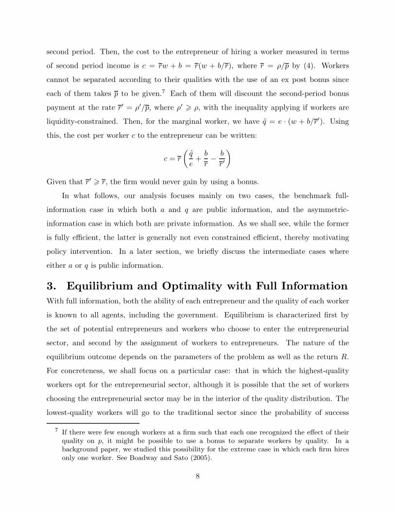
second period. Then, the cost to the entrepreneur of hiring a worker measured in terms

of second period income is c = rw + b = r(w + b/r), where r = ρ/p by (4). Workers

cannot be separated according to their qualities with the use of an ex post bonus since

each of them takes p to be given.7 Each of them will discount the second-period bonus

payment at the rate r′ = ρ′/p, where ρ′ � ρ, with the inequality applying if workers are

liquidity-constrained. Then, for the marginal worker, we have q = e · (w + b/r′). Using

this, the cost per worker c to the entrepreneur can be written:

c = r

(q

e+

b

r− b

r′

)Given that r′ � r, the firm would never gain by using a bonus.

In what follows, our analysis focuses mainly on two cases, the benchmark full-

information case in which both a and q are public information, and the asymmetric-

information case in which both are private information. As we shall see, while the former

is fully efficient, the latter is generally not even constrained efficient, thereby motivating

policy intervention. In a later section, we briefly discuss the intermediate cases where

either a or q is public information.

3. Equilibrium and Optimality with Full InformationWith full information, both the ability of each entrepreneur and the quality of each worker

is known to all agents, including the government. Equilibrium is characterized first by

the set of potential entrepreneurs and workers who choose to enter the entrepreneurial

sector, and second by the assignment of workers to entrepreneurs. The nature of the

equilibrium outcome depends on the parameters of the problem as well as the return R.

For concreteness, we shall focus on a particular case: that in which the highest-quality

workers opt for the entrepreneurial sector, although it is possible that the set of workers

choosing the entrepreneurial sector may be in the interior of the quality distribution. The

lowest-quality workers will go to the traditional sector since the probability of success

7 If there were few enough workers at a firm such that each one recognized the effect of theirquality on p, it might be possible to use a bonus to separate workers by quality. In abackground paper, we studied this possibility for the extreme case in which each firm hiresonly one worker. See Boadway and Sato (2005).

8

will be too low in the entrepreneurial sector. For example, no entrepreneur would hire a

worker with q = 0, since p = 0 in that case. (The highest-ability entrepreneurs will always

enter the sector.) In the case where the highest-quality workers enter, the nature of the

equilibrium outcome is intuitive.

Consider first the optimal matching of workers by quality with entrepreneurs by ability.

The probability of success for a type-a entrepreneur employing a set of workers q is p(a, q) =

βaqα, where a and each element of q are public information, and therefore qα and p are

known to the workers and the banks. For a given distribution of worker qualities and

entrepreneurial abilities in the entrepreneurial sector, aggregate expected output will be

highest if higher-quality workers are matched with higher-ability entrepreneurs. To see

this, consider two entrepreneurs of ability a2 > a1 and two sets of workers, q1

and q2,

whose qualities are such that qα2 > qα

1. Thus, workers q2

are of higher quality than q1

in

the sense that their average value of qα is higher. Expected output will be highest if qα2

is matched with a2, and qα1 with a1, since:

βa1qα1R + βa2qα

2R > βa1qα2R + βa2qα

1R, or a2(qα2 − qα

1) > a1(qα2 − qα

1)

Extending this logic to many types of entrepreneurs, output will be maximized by matching

the highest-quality workers with the highest-ability entrepreneurs. In our context where

the distributions of entrepreneurs and workers are uniform, and there are n workers for each

entrepreneur, matching will be perfect. Each entrepreneur will hire n workers of identical

quality, and workers of higher quality will be matched with entrepreneurs of higher ability.

Next, consider how the market might generate such an outcome. With full informa-

tion, wage rates will be specific to workers’ abilities, so there will be no adverse selection

and no involuntary unemployment (unlike in the asymmetric-information case as we shall

see in the next section). Therefore, there will be an equal number of workers and jobs in

the entrepreneurial sector (n per entrepreneur). Given that the densities of q and a are

identical by assumption, we might expect that the full-information equilibrium will en-

tail perfect matching of workers to entrepreneurs with q increasing in a. Moreover, if the

highest-ability entrepreneurs and the highest-quality workers are the ones that opt for the

entrepreneurial sector, which is the case we shall assume, the matching outcome will imply

9

q = a since the upper support of both distributions is the same. We proceed by showing

that q = a is in fact an equilibrium in the full-information case when both entrepreneurs

and workers are drawn from the top of their respective distributions. The cutoff ability of

active entrepreneurs will then be determined by a zero-net-expected-profit condition, and

since each entrepreneur hires n workers, that will determine the cutoff quality of workers

in the entrepreneurial sector.

To see that perfect matching will be an equilibrium, suppose the wage function is

w(q), where w(q) � q to ensure participation. Consider an entrepreneur of type a, and

suppose that entrepreneur hires n(q) workers of type q, where∫ 1

0n(q)dq = n. Given that

a and q are public information, the banks charge an entrepreneur-specific gross interest

rate of r(p) = ρ/p, where by (1):

p(a, q) = βa

∫ 1

0n(q)qαdq

n

Then given the wage function w(q), the entrepreneur’s expected profits can be written,

using (2) and (3), as:

(6) π = p(a, q)(

R − r

∫ 1

0

w(q)n(q)dq

)= βaR

∫ 1

0n(q)qαdq

n− ρ

∫ 1

0

w(q)n(q)dq

Entrepreneurs choose their mix of workers to maximize expected profits, given the wage

function w(q).

Suppose the wage function w(q) determined by the market for workers is convex, so

w′′(q) � 0. We shall confirm below that this will be the case in equilibrium. Then, the

following lemma applies:8

Lemma 1: If w′′(q) � 0, then entrepreneur a prefers to hire all n workers of the same

quality q∗:

n∗(q) = n for q = q∗

8 Proof: Expected profits in (6) may be written π = βaRE[qα] − ρnE[w(q)]. Then sinceE[qα] < E[q]α for α < 1 and E[w(q)] � w (E[q]) for w′′(q) � 0, we have π = βaRE[qα] −ρnE[w(q)] < βaRE[q]α − ρnw (E[q]). Therefore, starting in a situation in which workersof different qualities are hired, the entrepreneur can increase profits by replacing them withn workers of a type equal to the average quality of existing workers, q = E[q], since thenexpected profits will be βaRE[q]α − ρnw (E[q]).

10

n∗(q) = 0 for q �= q∗

Given that entrepreneurs all hire workers of a single quality, expected profits (6) can

be rewritten

(6′) π(a, q) = βaRqα − ρnw(q)

It must also be the case that, since there are n workers of each quality, all entrepreneurs

hire a different quality of worker. With workers being drawn from the top of the quality

distribution, we expect that q = a will be an equilibrium. This will be so if profits π(a, q)

are maximized where q = a. The first-order condition for an entrepreneur a’s choice of q

is:∂π(a, q)

∂q= βaRαqα−1 − ρnw′(q) = 0

This will be satisfied at q = a if:

(7) w′(q) =αβR

ρnqα

The second-order condition for the entrepreneur’s problem, evaluated at q = a, is:

∂2π(a, a)∂q2

= βaR(α − 1)αqα−2 − ρnw′′(q) < 0

Since the first term is negative, this will be satisfied if w′′ � 0, which by (7) is the case.

Thus, q = a is clearly a candidate for equilibrium since it can be supported by a wage

function satisfying (7).

To verify that q = a is an equilibrium, we can obtain an expression for the wage

function w(q) by integrating (7) to obtain:

(8) w(q) =αβR

ρn(1 + α)qα+1 + F

where F is a constant of integration, whose value will be determined below. We assume

that w(q) is defined over [0, 1] and is a continuous function. Moreover, we assume that R

is sufficiently large that in (7), w′(q) > 1 for all workers in the entrepreneurial sector. In

fact, this will be the case if w′(q) > 1 for the marginal worker, since w′(q) is increasing in

11

q along the wage profile defined by (8). This is sufficient to ensure that the highest-quality

workers are the ones that enter the entrepreneurial sector.

Let q be the ability of the marginal worker. Then, competition for workers will ensure

that w(q) = q, where q is the wage rate that can be obtained in the traditional sector.9

Since w′(q) > 1, w(q) > q for all workers with q > q, implying that the highest-quality

workers enter the entrepreneurial sector. (Of course, had it been the case that w′(q) < 1

for the marginal worker, a segment of workers from the interior of the wage distribution

would enter.) Since, as we shall confirm below, the highest-ability entrepreneurs are the

active ones, the marginal entrepreneur with lowest ability a will hire the marginal workers

q. And, since the densities of the two distributions are the same, this implies that q(a) = a

so there is perfect matching. Therefore, from w(q) = q = a, we can infer by applying (8)

for the marginal workers that F satisfies:

(9) F = a − αβR

ρn(1 + α)aα+1

The wage profile will adjust so that (9) is satisfied. All workers with q > a will therefore

earn w(q) > q by (8) and the fact that w′(q) > 1, implying that they will earn a surplus.

Consider now the entrepreneurs. The expected profit of an entrepreneur of ability a

is given by: π = βaqαR − ρnw(q), where w(q) satisfies (8) and (9). The solution to the

entrepreneur’s first-order condition will be q = a, and it will be unique since the second-

order condition for the entrepreneur’s problem is satisfied. Therefore, expected profits may

be written:

π(a) = βa1+αR − ρn

(αβR

ρn(1 + α)aα+1 + F

)=

βR

(1 + α)aα+1 − ρnF

where F is given by (9). Since π(a) is increasing in a, that implies that the marginal

entrepreneur will have the lowest ability among active entrepreneurs. The ability of the

marginal entrepreneur a is determined, using (9), by:

(10) π0 = βRaα+1 − ρna

9 To see this, note that if w(q) > q, a worker of slightly lower quality, say q − ε, can offer towork for a slightly lower wage. The marginal entrepreneur would then prefer to employ thisworker than one with quality q.

12

All entrepreneurs with a � a will enter, and the number of active entrepreneurs, denoted

m, will be given by m = 1 − a.

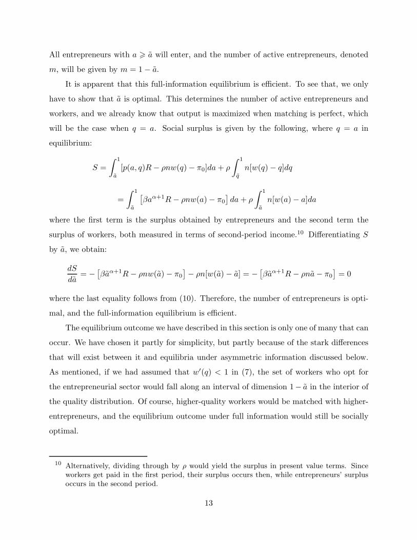
It is apparent that this full-information equilibrium is efficient. To see that, we only

have to show that a is optimal. This determines the number of active entrepreneurs and

workers, and we already know that output is maximized when matching is perfect, which

will be the case when q = a. Social surplus is given by the following, where q = a in

equilibrium:

S =∫ 1

a

[p(a, q)R − ρnw(q) − π0]da + ρ

∫ 1

q

n[w(q) − q]dq

=∫ 1

a

[βaα+1R − ρnw(a) − π0

]da + ρ

∫ 1

a

n[w(a) − a]da

where the first term is the surplus obtained by entrepreneurs and the second term the

surplus of workers, both measured in terms of second-period income.10 Differentiating S

by a, we obtain:

dS

da= − [

βaα+1R − ρnw(a) − π0

] − ρn[w(a) − a] = − [βaα+1R − ρna − π0

]= 0

where the last equality follows from (10). Therefore, the number of entrepreneurs is opti-

mal, and the full-information equilibrium is efficient.

The equilibrium outcome we have described in this section is only one of many that can

occur. We have chosen it partly for simplicity, but partly because of the stark differences

that will exist between it and equilibria under asymmetric information discussed below.

As mentioned, if we had assumed that w′(q) < 1 in (7), the set of workers who opt for

the entrepreneurial sector would fall along an interval of dimension 1− a in the interior of

the quality distribution. Of course, higher-quality workers would be matched with higher-

entrepreneurs, and the equilibrium outcome under full information would still be socially

optimal.

10 Alternatively, dividing through by ρ would yield the surplus in present value terms. Sinceworkers get paid in the first period, their surplus occurs then, while entrepreneurs’ surplusoccurs in the second period.

13

4. Equilibrium with Asymmetric InformationIn this case, both a and q are private information. All workers who are employed in the

entrepreneurial sector obtain a common wage rate w, while all active entrepreneurs face a

common interest rate r. We begin with a general overview of the relationships that must

hold in equilibrium before turning to the qualitative features of equilibria.

Equilibrium Relationships

Consider first the decision of workers to seek employment in the entrepreneurial versus the

traditional sector. Suppose workers believe—correctly in equilibrium—that the probability

of being employed in the entrepreneurial sector is e. All entrepreneurs will offer the same

wage rate w in equilibrium since all workers have the same expected quality from the point

of view of entrepreneurs. Given w, the expected income of workers in the entrepreneurial

sector is ew. Since a worker of quality q can receive a wage of q in the traditional sector,

the cutoff quality of workers by (5) is q = ew. All workers with q < q—those with

the lowest quality—choose the entrepreneurial sector regardless of the parameters of the

problem. This is in contrast with the social optimum achieved with full information where a

segment of higher-quality workers will generally be attracted to the entrepreneurial sector.

Each entrepreneur also takes e as given. Recall from (1) that the probability of success

for an entrepreneur depends on qα, which cannot be observed here. When an entrepreneur

hires workers, those workers are selected randomly from the pool of available workers with

q ∈ [0, q], so E[qa] is the same for all entrepreneurs. Given e and the uniform distribution

of workers, E[qa] is given by:

(11) E[qa] = E [qα|q � q] =1q

∫ q

0

qαdq =qα

1 + α=

(ew)α

1 + α

Then, for an entrepreneur of ability a, the expected probability of success will be given by

(12) E[p] = βaE[qa] =βa

1 + α(ew)α

Expected profits for this entrepreneur can therefore be written, using (2), as:

(13) π = E[p](R − rnw) =βa

1 + α(ew)α(R − rnw)

14

This assumes that all entrepreneurs who choose to become active can receive a loan at

the rate r. We return later to the issue of whether there can be credit rationing in this

context, which would complicate matters considerably.

Each active entrepreneur can be thought of as choosing a wage rate to maximize prof-

its, given e. All entrepreneurs who become active offer the same wage rate w in equilibrium,

as we shall confirm. Moreover, workers will be indifferent among active entrepreneurs since

they are paid the wage w in advance, so are not affected by bankruptcy. Let m be the

number of active entrepreneurs. Since there are nq workers in the entrepreneurial sector

and since each entrepreneur hires n workers, the employment rate e is given by:

(14) e = min{

nm

nq, 1

}= min

{m

q, 1

}For the case in which m < q, there is unemployment (e < 1) and we have by (5) and (14),

q = ew = mw/q. Therefore, the labor force in the entrepreneurial sector and the rate of

employment can be expressed respectively as q =√

mw and e =√

m/w. This implies

that the quality of the marginal worker with full employment and unemployment may be

written:

(15) q = ew =

⎧⎨⎩ w if m = w

√mw if m < w

Banks can observe neither a nor q. Assuming that projects are allocated randomly

among banks, the interest rate they offer will be r = ρ/p by (4), where p is the expected

probability of success of any given project. Using (12) and (15), p is given by:

(16) p =

⎧⎨⎩βa

1+αwα if m = w

βa1+α(mw)

α2 if m < w

where a is the average quality of active entrepreneurs, discussed below. Expected profits

of an entrepreneur of ability a in equilibrium can then be written, using (13) and (15), as:

(17) π =

⎧⎨⎩βa

1+αwα(R − rnw) if m = w

βa1+α (mw)

α2 (R − rnw) if m < w

15

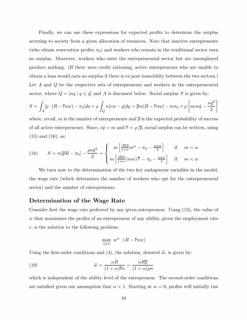
Finally, we can use these expressions for expected profits to determine the surplus

accruing to society from a given allocation of resources. Note that inactive entrepreneurs

(who obtain reservation profits π0) and workers who remain in the traditional sector earn

no surplus. Moreover, workers who enter the entrepreneurial sector but are unemployed

produce nothing. (If there were credit rationing, active entrepreneurs who are unable to

obtain a loan would earn no surplus if there is ex post immobility between the two sectors.)

Let A and Q be the respective sets of entrepreneurs and workers in the entrepreneurial

sector, where Q = [nq | q � q] and A is discussed below. Social surplus S is given by:

S =∫

A

[p · (R− rnw)− π0]da + ρ

∫Q

n[ew − q]dq = pm[R− rnw]−mπ0 + ρ

[newq − nq2

2

]where, recall, m is the number of entrepreneurs and p is the expected probability of success

of all active entrepreneurs. Since, eq = m and r = ρ/p, social surplus can be written, using

(15) and (16), as:

(18) S = m[pR − π0] − ρnq2

2=

⎧⎪⎨⎪⎩m

[βaR1+α

mα − π0 − ρnm2

]if m = w

m[

βaR1+α

(mw)α2 − π0 − ρnw

2

]if m < w

We turn now to the determination of the two key endogenous variables in the model,

the wage rate (which determines the number of workers who opt for the entrepreneurial

sector) and the number of entrepreneurs.

Determination of the Wage Rate

Consider first the wage rate preferred by any given entrepreneur. Using (13), the value of

w that maximizes the profits of an entrepreneur of any ability, given the employment rate

e, is the solution to the following problem:

max{w}

wα · (R − rnw)

Using the first-order conditions and (4), the solution, denoted w, is given by:

(19) w =αR

(1 + α)rn=

αRp

(1 + α)ρn

which is independent of the ability level of the entrepreneur. The second-order conditions

are satisfied given our assumption that α < 1. Starting at w = 0, profits will initially rise

16

with w and eventually reach a peak at w, assumed to be at w < 1 so that we have an

interior solution. The intuition here is that the rise in w attracts better quality workers,

which increases the probability of success, but also increases labor costs. Given that p is

concave in q, the latter eventually offsets the former.

Denote by we the market clearing, or equilibrium wage rate, that is, the wage rate

such that e = 1. Given m, the market clearing wage will be we = m, where the number of

workers just equals the number of entrepreneurs, q = m. Whether involuntary unemploy-

ment exists depends upon the relative size of we and w. If w > we = m, entrepreneurs

will bid up the wage rate above the market clearing level, attracting excess workers into

the entrepreneurial sector and generating involuntary unemployment. On the other hand,

if w � we = m, the wage rate will be bid up only to we by competition for workers, so

there will be full employment. Consider the consequences for entrepreneurial profits of

each outcome in turn.

Unemployment Case: w > we = m

In this case, the market wage is w given by (19) and p is given by the second row of (16).

These consist of two equations in w and p whose solutions are:

(20) p(a, m) =(

βa

1 + α

) 22−α

(α

1 + α

mR

ρn

) α2−α

(21) w(a, m) =[

βa

1 + α

α

1 + α

R

ρn

] 22−α

mα

2−α

where both p(a, m) and w(a, m) are increasing in a and m.

The expected profits of an entrepreneur of ability a can be written as follows, using

the second row of (17) with w = w:

π =βa(mw)

α2

1 + α(R − rnw)

Using (21), this yields:

(22) π(a, a, m) = a

(β

1 + α

R

1 + α

) 22−α

(αam

ρn

) α2−α

17

where π(·) refers to expected profits when the wage rate is w. This function for expected

profits is increasing in all three arguments, a, a and m.

Full Employment Case: w � we = m

In this case, by the first row of (16), we have

p =βamα

1 + α

Expected profits of an entrepreneur of ability a can immediately be written, using r = ρ/p

and the above expression for p, as:

(23) πe(a, a, m) =βamα

1 + α(R − rnm) = a

(βRmα

1 + α− ρnm

a

)In this case, πe(·), expected profits when w = we, is increasing in a and a, but the effect

of m is ambiguous.

The Number of Active Entrepreneurs

Given that expected profits are increasing in ability a with or without unemployment, there

is a cutoff ability level a such that all entrepreneurs with a � a become active and the

remainder obtain their reservation profits π0. Then, the number of active entrepreneurs

is m = 1 − a, and given the uniform distribution that we have assumed, their average

(expected) ability is a = (1 + a)/2, so

(24) m = 2 − 2a

Recall from (21) that the profit-maximizing wage rate w depends on a and m. There-

fore, whether w � we = m depends on a. In particular, using (21) and (24), we obtain

that:

(25) w > we ⇐⇒ βa

1 + α

α

1 + α

R

ρn> (2 − 2a)1−α

The left-hand side of (25) is increasing in a, while the right-hand side is decreasing. More-

over, at a = 0, the right-hand side exceeds the left-hand side. Therefore, there will be a

value of a, denoted a′ such that

(26)βa′

1 + α

α

1 + α

R

ρn= (2 − 2a′)1−α

18

For a � a′, w � we (there is full employment), and vice versa. It must be the case that

0 < a′ < 1 (since the right-hand side is less that the left-hand side at a = 1). Note that

a � 1/2 since if m = 0, a = 1/2. In what follows, we shall assume that a′ > 1/2 to allow

for the possibility that there is full employment. If a′ < 1/2, a would always exceed a′ so

there would always be involuntary unemployment.

Whether the equilibrium involves full employment or unemployment depends on the

relationship between a and a′. In turn, the market wage w as well as the expected proba-

bility of success p and expected profits π depend on this relationship. We can summarize

these results for future reference as follows:

(27.1) w(a) =

⎧⎨⎩ m if a � a′

w(a, m) if a > a′

(27.2) p(a) =

⎧⎪⎨⎪⎩βamα

(1+α)if a � a′

(βa

1+α

) 22−α

(α

1+αmRρn

) α2−α

if a > a′

(27.3) π(a, a) =

⎧⎪⎨⎪⎩a

(βRmα

1+α − ρnma

)if a � a′

a(

β1+α

R1+α

) 22−α

(αamρn

) α2−α

if a > a′

where w(a, m) is given by (21), a′ is given by (26) and m = 2 − 2a by (24).

It remains to determine a, the average quality of entrepreneurs, which depends upon

how many entrepreneurs become active. For the marginal entrepreneur, π(a, a) = π0.

By (27.3), for a > a, we have π(a, a) > π0 since π(a, a) is increasing in a, confirming

our presumption that active entrepreneurs are those such that a � a. In characterizing

the number of active entrepreneurs, we can focus on the expected profit function for the

marginal entrepreneur, defined as π(a) ≡ π(a, a).

Using (27.3), we obtain

(28) π(a) = π(a, a) =

⎧⎪⎨⎪⎩a

[βR(2−2a)α

1+α − ρn(2−2a)a

]if a � a′

a[

β1+α

R1+α

] 22−α

[αa(2−2a)

ρn

] α2−α

if a > a′

19

where a = 2a − 1. Differentiating π(a) with respect to a gives:

(29)dπ(a)

da=

∂π(a, a)∂a

∂a

∂a+

∂π(a, a)∂a

= 2∂π(a, a)

∂a+

∂π(a, a)∂a

The first term on the right-hand side of (29) is positive since ∂π/∂a > 0. The second term,

∂π/∂a, is initially positive and then becomes negative, as differentiation will confirm.

Moreover, at a = 1/2 and a = 1, π(a) = 0. A typical shape for the π(a) function might be

single-peaked as shown in Figure 1.11

Interior equilibrium values for a will be those such that π(a) = π0. Figure 1 depicts

possible equilibria. For given values of π0, there are generally two interior equilibria, one

stable and the other unstable. The stable one is denoted a∗, and is to the left of the peak

of the π(a) curve. The other equilibrium au is unstable: for a > au, entrepreneurs will

exit causing a to rise, and vice versa. That implies that the two stable equilibria will be

the interior one at a = a∗ and the corner equilibrium a = 1 (where there are no active

entrepreneurs).12 Depending on the size of a relative to a′, the stable equilibrium may

involve unemployment. The higher the value of π0, the higher will be a∗, and the more

likely will there be unemployment in equilibrium.

The Possibility of Credit Rationing

Stiglitz and Weiss (1981) found that credit rationing could arise when projects were pooled

by their expected return (pR), which was exogenously given. In the de Meza and Webb

(1987) case where projects were pooled by their return R and the distribution of the prob-

ability of success p across entrepreneurs was given, credit rationing could not arise. Our

model is an extension of the de Meza-Webb model to allow for p for a given entrepreneur

to be endogenously determined by the quality of workers hired. It turns out that in this

case, credit rationing might arise. We simply show that possibility here without exploiting

its consequences for the form of equilibrium achieved and its efficiency properties.

11 Twice differentiating (28) with respect to a, we obtain that for a > a′, d2π/da2 < 0. However,

for a < a′, the sign of d2π/da2 is ambiguous. Differentiating (28) with respect to a also revealsthat π(a) can be increasing at a = a′ as shown in Figure 1. In fact, the slope of π(a) willgenerally be discontinuous at the point a = a′, but it can either rise of fall discontinuously.

12 Of course, if π0 is very high, the only equilibrium will be one in which there are no en-trepreneurs. In Figure 2, the π0 curve lies above the peak of the π(a) curve. We are rulingthis out as being not interesting for our purposes.

20

Consider first the marginal entrepreneur. Using ρ = r p by (4) and the expressions

for p in (27.2), the expected profits for the marginal entrepreneur in (28) can be rewritten

as follows:

(30) π(a, r) =

⎧⎪⎨⎪⎩(2a−1)β

1+α (2 − 2a)α(R − (2 − 2a)rn) if a � a′

(2a−1)βR(1+α)2

[αR(2−2a)(1+α)rn

]α2

if a > a′

where, in equilibrium, π(a, r) = π0. Suppose we focus on a stable interior equilibrium,

which requires that ∂π(a, r)/∂a > 0. Differentiating condition π(a, r) = π0, we obtain:

da

dr

∣∣∣∣π=π0

= −∂π/∂r

∂π/∂a

∣∣∣∣π=π0

> 0

where the sign follows from the stability condition and the fact that π(a, r) in (30) is

decreasing in r. Intuitively, an increase in the interest rate pushes the lowest-ability en-

trepreneurs out of the sector and increases the average quality of those remaining, a.

Next, turn to the banks. The expected profit per unit of lending is ΠB = p r − ρ.

Using (27.2) and the fact that m = 2−2a by (24), expected profits per unit can be written:

(31) ΠB =

⎧⎪⎨⎪⎩β2α

(1+α)a(1 − a)αr − ρ if a � a′

β1+α

(2α

1+αRn

) α2

a(1 − a)α2 r1−α

2 − ρ if a > a′

Credit rationing can only occur if an increase in the interest rate r causes bank expected

profits to fall. Given that a is increasing in r as shown above, a necessary condition for this

is that ∂ΠB/∂a < 0. From (31), we find by differentiation that for the full employment

case where a � a′, ∂ΠB/∂a < 0 if a > 1/(1 + α), which is clearly possible. Similarly,

in the unemployment case, we obtain that ∂ΠB/∂a < 0 if a > 2/(2 + α), which is again

possible. Thus, unlike in the de Meza-Webb case, credit rationing could occur in our model.

Intuitively, p can fall in a since lower-quality workers are left in the entrepreneurial sector

when the number of entrepreneurs decreases (a increases). Exploring the consequences

of that would be rather complicated and would take us too far afield from our present

purpose, so in what follows we rule out credit rationing.

To summarize the results of this section, equilibrium in the asymmetric-information

case will have the following features. The highest-ability entrepreneurs and the lowest-

quality workers will enter the entrepreneurial sector, in contrast with the full-information

21

case. As well, workers will be randomly assigned to entrepreneurs contrary to the efficient

matching of the full-information case. All entrepreneurs will pay a common wage rate,

which will be paid up-front, and a single interest rate facing all firms. There will generally

be multiple equilibria, unless π0 is high enough to rule out an entrepreneurial sector entirely.

Two equilibria will be stable and one unstable. The stable equilibria will include one

interior one and one corner solution in which there are no entrepreneurs. The interior

stable equilibrium may or may not involve involuntary unemployment.

5. Efficiency and Policy with Asymmetric Information

In this section, we study the optimality properties of equilibrium outcomes with asymmet-

ric information in credit and labor markets. Our main interest will be in stable interior

equilibria with and without unemployment. We begin by investigating the efficiency of

market equilibria, and then look at the consequences for government policy.

Local Efficiency Properties of Equilibria

Recall the expressions for social surplus S in (18). Rewriting these using the fact that

m = 2 − 2a, we obtain:

(32) S =

⎧⎪⎨⎪⎩(2 − 2a)

[βaR1+α (2 − 2a)α − π0 − (1 − a)ρn

]if a � a′

(2 − 2a)[

βaR1+α(2 − 2a)

α2 w

α2 − π0 − ρnw

2

]if a > a′

where w in the case of unemployment is given by (21), with m = 2− 2a. The efficiency of

the equilibrium outcomes can be investigated by considering the effects on social surplus of

incremental changes in a and, in the case of an unemployment equilibrium, in w. Consider

the unemployment case first, concentrating on the interior equilibrium (a < 1).

Unemployment Equilibrium: 1 > a > a′

In this case, S depends on a directly and also indirectly via w(a). Consider the two effect

in turn. Differentiating the second row in (32) partially with respect to a, we obtain, after

22

straightforward manipulation and using the expressions for p and w in (27.2) and (19):13

(33)∂S

∂a

∣∣∣∣w

=[2a− 4 − α

]ρnw < 0

where the sign follows from the fact that a > 1/2. Then, differentiating S with respect to

w and using (27.2), (24) and (19), we obtain:

(34)∂S

∂w

∣∣∣∣a

=αρnm

2> 0

Thus, (33) and (34) indicate that an unemployment equilibrium is inefficient. If a and

w could be manipulated separately, a should be reduced (the number of entrepreneurs

increased) and w should be increased (more high-ability workers should be attracted into

the entrepreneurial sector).

However, w depends on a through (21). Substituting m = 2 − 2a in (21) and differ-

entiating with respect to a, we obtain:

∂w

∂a� 0 as

22 + α

� a

This relationship between w and a applies only for a > a′. For a � a′, full employment

exists, so w = m = 2 − 2a implying that w is declining in a. The two panels of Figure

2 depict possible cases for the relationship between the w and a, depending on whether

a′ � 2/(2+α). If a′ � 2/(2+α), the market wage is monotonically decreasing in a, while

if a′ < 2/(2+α), the wage rate is hump-shaped in the range where there is unemployment.

These figures will be useful again below.

13 Specifically, differentiating (32) and using (27.2), we obtain:

1

2

∂S

∂a

∣∣∣∣w

= pR(

1 − 2a

a

)+ π0 +

ρnw

2− αpR

2

Since a = 2a − 1, pa/a = p (by (1)), and p(R − ρnw/p) = π0 for the marginal entrepreneur,this becomes:

1

2

∂S

∂a

∣∣∣∣w

= ρnw(

1

a− 3

2

)− αpR

2

which reduces to the expression in the text using (19).

23

The total effect of a change in a on surplus can be expressed as follows:

(35)dS

da=

∂S

∂a+

∂S

∂w

∂w

∂a

Given (33) and (34), this will be unambiguously negative if ∂w/∂a < 0, which will be the

case if a > 2/(2 + α). That is, an increase in the number of entrepreneurs would increase

efficiency. Otherwise, it will be ambiguous. We return below to how policy might be used

to enhance efficiency.14

Full Employment Equilibrium: 1/2 < a � a′

With full employment, a has only a direct effect on S in the first row of (32). Differentiating

with respect to a, we obtain after similar manipulation:

(36)12

dS

da=

2ρn(1− a)2

a− αpR

To interpret this, use we = m = 2 − 2a and αpR = ρn(1 + α)w by (19) to find:

12

dS

da= ρn

(1 − a

awe − (1 + α)w

)� 0

since we > w. Thus, there may be too few or too many entrepreneurs in the full-

employment equilibrium.

These efficiency results contrast with those of de Meza and Webb (1987) who show

that in the absence of heterogeneous worker quality, there are unambiguously too many

entrepreneurs in equilibrium (a is too low in our notation). In the de Meza-Webb model,

there is an adverse selection effect that allows low-quality entrepreneurs to take advantage

of a common interest rate, and too many do so. That effect is present in our model as

well, but in addition the quality of workers hired in the entrepreneurial sector tends to

14 Note that an increase in the number of entrepreneurs will increase employment, even if italso increases w. To see this, use m = 2 − 2a and (21) to give:

e =√

m/w =

[(2 − 2a)1−

α2−α

(βa

1 + α

α

1 + α

R

ρ

) −22−α

] 12

Differentiating this with respect to a, we obtain de/da < 0.

24

be too low. Increasing the number of entrepreneurs is a way of attracting higher-quality

workers, but at the expense of taking lower-quality entrepreneurs. Either of those effects

can dominate.

The above welfare effects are local ones. Unfortunately in our model, social surplus

in (32) is not globally concave. Differentiation with respect to a indicates that d2S/da2 is

generally of ambiguous sign. Therefore, there are various possibilities for global optima,

as our discussion next illustrates.

Policy Implications

In the above analysis, we considered a hypothetical perturbation of a, and thus w in the

unemployment case, around the equilibrium. The government cannot control a directly

since that is determined by the decision of entrepreneurs to become active. Instead, in

a decentralized market economy, the government can influence equilibrium outcomes by

intervening with taxes or subsidies. Two kinds of policy instruments might be used to in-

fluence a and w: a tax or subsidy on entrepreneurs who become active and a tax or subsidy

on wages. We begin by analyzing how these policy instruments affect equilibrium values of

a and w. Then, we turn to the effect of policies on the social surplus, S. In evaluating the

potential for policy intervention, it is useful to note that since the government can observe

neither the quality of workers nor the ability of entrepreneurs, the full-information opti-

mum cannot be achieved. In particular, workers cannot be optimally matched to firms,

and nothing can be done to avoid the fact that it will be the lowest quality of workers

that will be attracted to the entrepreneurial sector. A more far-reaching analysis might

consider ways in which information about q and a could be elicited, such as by signaling

or ex ante monitoring.

Effect of Policies on Equilibrium Outcomes

Let τ be a subsidy on entrepreneurs, and σ a wage subsidy. Then, (2) can be revised to

give the after-subsidy expected profit of an active entrepreneur:

π = E[p](R − (1 − σ)nwr) + τ � π0

where E[p] = βa(ew)α/(1 + α) by (12) and r = ρ/p by (4). The equilibrium value of a

25

is determined by the zero-net-profit condition of the marginal entrepreneur. Revising (28)

to incorporate the subsidies and using a = 2a − 1, we obtain:

(37) π(a, σ, τ) =

⎧⎪⎨⎪⎩(2a − 1)

[βR(2−2a)α

1+α − (1−σ)ρn(2−2a)a

]+ τ if a � a′

(2a − 1)[

β1+α

R1+α

] 22−α

[αa(2−2a)(1−σ)ρn

] α2−α

+ τ if a > a′

where π(a, σ, τ) = π0 in equilibrium. Equation (37) determines how a, and therefore a

responds to changes in σ and τ . Let us focus on the stable interior solution in Figure 1.

Stability requires that ∂π/∂a > 0 for both the full employment and unemployment cases.

Since ∂π/∂σ > 0 and ∂π/∂τ > 0 in (37), we have that:

(38)∂a

∂σ= −∂π/∂σ

∂π/∂a< 0,

∂a

∂τ= −∂π/∂τ

∂π/∂a< 0

which imply that ∂a/∂σ < 0 and ∂a/∂τ < 0 as well. An increase in either subsidy

increases the number of active entrepreneurs by attracting more low-ability ones into the

entrepreneurial sector.

Next, consider the wage rate. In the full employment case, the market-clearing wage is

w = m = 2−2a as before. An increase in the number of entrepreneurs reduces a and there-

fore w. Lower-ability entrepreneurs and lower-quality workers enter the entrepreneurial

sector.

With unemployment, the preferred wage rate in (19) becomes:

(19′) w =αRp

(1 − σ)(1 + α)ρn

which, combined the expression for p in (16), then leads to a revised version of (21):

(21′) w(a) =[

β

1 + α

α

1 + α

R

(1 − σ)ρn

] 22−α

[a2(2 − 2a)α]1

2−α

In equilibrium, a will be determined by π(a, σ, τ) = π0 in (37). Combining the second row

in (37) with (21′) yields w as a function of the equilibrium value of a and the subsidies:

(39) w(a, τ, σ) =(π0 − τ)α(1 − σ)ρn

a

2a − 1if a∗ > a′

26

where

(40)∂w

∂a< 0,

∂w

∂τ< 0,

∂w

∂σ> 0

We are now in a position to investigate the effect of subsidy policy on social surplus.

We begin with local welfare analysis, evaluating the effect of introducing small subsidies

starting at laissez-faire equilibria. Then, optimal policies are considered.

The Efficiency Effect of Incremental Policies

Social surplus is again given by (32), where now a and w depend on τ and σ. We consider

the effect of changes in τ and σ on S in the unemployment and the full-employment

equilibria in sequence.

Unemployment Case

Differentiating the second row of (32) with respect to a and w and using (27.2) and (19′),

we obtain the analogs of (33) and (34):15

(41)∂S

∂a=

[2a− 4 − α +

σ

1 − σ

](1 − σ)ρnw + 2τ

(42)∂S

∂w

∣∣∣∣a

= [α − (1 + α)σ]mρn

2

At the no-subsidy equilibrium with τ = σ = 0, these reduce to (33) and (34) with ∂S/∂a <

0 and ∂S/∂w > 0.

Consider now the effect of small changes in subsidies on social surplus. Differentiating

the second row in (32) with respect to τ and σ yields:

(43)∂S

∂τ=

∂S

∂a

∂a

∂τ+

∂S

∂w

dw

dτ,

∂S

∂σ=

∂S

∂a

∂a

∂σ+

∂S

∂w

dw

dσ

where dw/dτ and dw/dσ include both the direct effects of these policies on w by (40)

and the indirect effect through changes in a using (38). These imply dw/dτ � 0 and

15 We are assuming an interior solution with w < 1, although technically a corner solution withall workers choosing the entrepreneurial sector is possible.

27

dw/dσ > 0. Suppose we evaluate this starting at the no-intervention equilibrium. Then,

using the signs obtained from (41) and (42) when τ = σ = 0, we obtain:

∂S

∂τ

∣∣∣∣τ=σ=0

� 0,∂S

∂σ

∣∣∣∣τ=σ=0

> 0

Thus, starting from the laissez-faire unemployment equilibrium, welfare will be unambigu-

ously increased if we impose a small subsidy on wages.

Full Employment Case

In this case, S depends only on a. Differentiating the first row of (32) with respect to a

and using (27.2) yields the analog of (36) with subsidies incorporated:

(44)12

dS

da=

2ρn(1 − a)2

a− αpR + σρn

(2a− 1)(2 − 2a)a

+ τ

This again reduces to (36) and has an ambiguous sign in the no-intervention case.

The effects of small changes in τ and σ on social surplus are now:

(45)∂S

∂τ=

dS

da

∂a

∂τ,

∂S

∂σ=

dS

da

∂a

∂σ

Both of these have ambiguous signs at the no-intervention full-employment equilibrium.

Optimal Policies

Suppose now that the government can choose subsidies σ and τ to maximize social surplus.

It turns out that the social optimum may involve either full employment or unemployment

depending on the parameters of the problem.

If the optimum involves unemployment, the government will choose τ and σ such

that in (43), ∂S/∂τ = ∂S/∂σ = 0. This will be the case if ∂S/∂a = 0 and ∂S/∂w = 0,

where these are given by (41) and (42). This leads to a straightforward characterization

of optimal policies. Setting (42) to zero, we immediately obtain the optimal wage subsidy:

σ =α

1 + α> 0

Then, setting (41) to zero and using this expression for σ (which implies that σ/(1−σ) = α),

the optimal subsidy on entrepreneurs satisfies:

∂S

∂a=

[2a− 4

](1 − σ)ρnw + 2τ = 0 =⇒ τ > 0

28

where the sign of τ follows from the fact that a > 1/2. Thus, if unemployment exists in

the optimum, both the wage subsidy and the subsidy on entrepreneurs should be positive.

On the other hand, if the optimum involves full employment, S depends only on a.

Optimal subsidy policies require setting (44) to zero, and this requires only one policy

instrument. It is apparent that either τ or σ can be used. Here, the sign of the optimal

subsidy is ambiguous. Suppose, for example, that τ is used. Then, its sign depends on the

sign of the first two terms on the right-hand side of (44), or equivalently the right-hand

side of (36), which is ambiguous. This parallels the result found above for incremental

policy changes.

Whether there is full employment or unemployment in the optimum depends upon

the parameters of the problem. To see this, consider how S varies with a. In the case of

unemployment, differentiating the second row of (32) with respect to a and using (27.2),

we obtain:16

(46)∂S

∂a

∣∣∣∣a>a′

= pR

[2a− α − 4

]+ ρnw + 2π0

For the full employment case, we found earlier that differentiating the first row of (32)

gives:

(47)dS

da

∣∣∣∣a<a′

= pR

[2a− 2α − 4

]+ (2 − 2a)ρn + 2π0

As a approaches a′, we move from one case to the other. Let a → a′+ denote a approaching

a′ from above (in the unemployment region), and vice versa for a → a′−. Then we obtain

from (46) and (47), and using the fact that w = 2 − 2a at a = a′:

lima→a′+

dS

da− lima→a′

−

dS

da= αρnw > 0

Therefore, the slope of S(a) increases discontinuously at a = a′, implying that S(a) cannot

be concave. Moreover, whether the slope of S(a) at a = a′ is positive or negative depends

upon the parameters of the problem, as inspection of (46) and (47) indicates.

16 This is just the first equation in footnote 11. Note that we are assuming that σ is chosenoptimally so that ∂S/∂w = 0. Therefore, we need not take account of changes in w as achanges.

29

Suppose first that S(a) is single-peaked in a. Then, if ∂S/∂a < 0 at a = a′, it will be

optimal to induce a reduction in a thereby moving into the range of full employment. By

the same token, if ∂S/∂a > 0, there will be unemployment in the optimum. From (46) and

(47), we can see that ∂S/∂a will be positive at a = a′ if π0 is large enough. A large value

of π0 will make it more difficult to attract entrepreneurs into the sector, thereby increasing

the chances of an unemployment equilibrium.

However, it is quite possible that S(a) is not single-peaked. That is, lima→a′+dS/da

may be positive, while lima→a′−dS/da is negative. This can occur if the wage function is

as depicted in Panel B of Figure 2. Then, a reduction in a will cause S to rise. However,

starting at a = a′, increases in a will also cause w to rise in this case. This increase in

w together with the increase in a could cause the right-hand side of (46) to rise. There

would be local optima in both the full-employment and unemployment ranges of a, and

either one could be the global optimum.

Thus, policy prescriptions depend on the parameters of the problem: with unemploy-

ment both σ and τ should be positive, while with full employment only one of σ or τ

is needed and it could be positive or negative. Indeed, optimal policies are even more

ambiguous when we recall that the laissez-faire equilibrium could be a corner solution in

which no entrepreneurs are active. In this case, it will be necessary to impose sufficiently

large subsidies to move the initial equilibrium to a stable interior one. To study this case

properly would involve an explicitly dynamic analysis.

6. Alternative Information AssumptionsIn the previous analysis, we assumed that both worker qualities and entrepreneur abilities

were private information. This results in adverse selection in two markets, which leads to

various sorts of ambiguity: ambiguity about the possibility of unemployment, ambiguity

about policy prescriptions, and multiple equilibria. Moreover, equilibrium outcomes vary

considerably from the full-information case in terms of the quality of workers that opt for

the entrepreneurial sector, the number of entrepreneurs, and the mismatch between worker

quality and entrepreneurial ability. In this section, we relax the information assumptions

by allowing either a or q to be public information. In each case, we shall simply sketch

30

the outlines of the analysis and summarize the results rather than providing a full-fledged

treatment, which would be too space-consuming. The intuition will apparent given what

we have learned in the case already considered.

Entrepreneurial Ability Known

Suppose first that a is public information, but q remains private. Since workers cannot

be distinguished, a common wage w will be offered, and the expected quality of workers

employed by all entrepreneurs will be the same. Banks can offer ability-specific gross

interest rates r(a) = ρ/p(a), where p(a) is given by the expression for E[p] in (12). The

expected profit of a type-a entrepreneur then becomes:

(48) π = p(R − r(a)nw) =βaR(ew)α

1 + α− ρnw

where e � 1 is the employment rate for workers who opt for the entrepreneurial sector.

As before, entrepreneurs take e as given and choose a wage to offer. As we shall

see, each entrepreneur will have a different preferred wage rate, but competition among

entrepreneurs will cause a common wage rate to emerge (which may or may not clear the

labor market). To see this, consider the population of active entrepreneurs. Suppose that

all entrepreneurs with a � a will become active, and let w(a) be the wage offered by a

type-a entrepreneur. Workers who seek a job in the entrepreneurial sector will apply to

the entrepreneurs offering the highest w(a). We assume, critically, that there is ex post

immobility not only between sectors as above, but also from one entrepreneur to another

once a job application is made. This implies that competition for workers will equalize

w(a) among entrepreneurs, so we can simply write w in what follows. Given the probability

of employment e, workers with q � ew are attracted to the entrepreneurial sector, and all

are indifferent among the active entrepreneurs.

Suppose as before that there are m active entrepreneurs. In equilibrium, all en-

trepreneurs will perceive the same e (although out of equilibrium they may well perceive

different ones), and that will be given by (14) as before. Moreover, given that w is the same

for all entrepreneurs—the highest one preferred by any active entrepreneur—the equilib-

rium wage rate will again be given by w with q =√

mw if there is unemployment by (15),

and we = m if there is full employment. Unemployment will occur if w > we as before.

31

Consider now what determines the common value of w that is offered by all en-

trepreneurs in the unemployment case. Given e, an entrepreneur of ability a prefers the

wage rate w that maximizes expected profits π given by (48). The solution to this problem

yields:

w(a) =(

βaRα

(1 + α)ρn

)1/(1−α)

eα/(1−α)

which is increasing in a. The entrepreneur with a = 1 prefers to offer the highest wage

rate, and all other entrepreneurs will be obliged to follow. Therefore, w = w(1). As long

as w > m, that will be the prevailing wage rate. In effect, perfect information in capital

markets intensifies competition for workers thereby pushing up w. Using e =√

m/w, the

above equation for entrepreneur a = 1 becomes:

(49) w =(

βRα

(1 + α)ρn

)2/(2−α)

mα/(2−α)

The characterization of equilibrium is similar to that for the asymmetric-information

case considered earlier. The market clearing wage rate will be we = m, where m = 2− 2a.

There will be a value of a, say a′, such that w = we. The equilibrium wage rate will be

w = we if a � a′, and w = w if a > a′, where w is given by (49). We can proceed as above

to derive expected profits for the marginal entrepreneur, π(a), the analog of (28). The

analog of Figure 1 applies here as well. There will generally be two interior equilibria, only

one of which is stable. The other stable equilibrium is that at which a = 1 where there are

no active entrepreneurs. In the stable equilibrium, there may be either full employment or

unemployment.

It is apparent that this case has similar qualitative features to the asymmetric-

information case analyzed earlier. In both cases, there may be full employment or involun-

tary unemployment. Workers are paid a common wage and are drawn from the bottom of

the quality distribution. There is, however, no adverse selection problem in credit markets

in the sense that the interest rate can be conditioned on the ability of entrepreneurs. This

implies some differences in the equilibrium possibilities under the two regimes. It will be

the case that a′ will be lower and w higher in this case than in the case where both a and

q are private information. This is a consequence of the fact that the wage rate is bid up to

32

that preferred by the highest-ability entrepreneur. If there is full employment, wage rates

will be the same for a given number of entrepreneurs. Unfortunately, although one might

expect there to be fewer entrepreneurs financed in this case given the absence of adverse

selection, that turns out not to be unambiguously the case. Nonetheless, from a social

point of view, the number of entrepreneurs is now unambiguously too low (a is too high)

if there is full employment: the tendency for over-entry due to adverse selection in credit

markets (the De Meza-Webb effect) no longer applies.

Worker Quality Known

In this case, worker quality can be observed by all agents, but each entrepreneur’s ability

is private knowledge. This information structure leads to a somewhat more complicated

outcome. Since the qualities of the workers hired by a given entrepreneur are known to

the bank, the interest rate charged can reflect those qualities. Consider an entrepreneur

that hires n(q) workers of quality q, where∫

n(q)dq = n as before. The gross interest rate

charged to this entrepreneur is r = ρ/p(q) with p(q) = βaqα, where qα =∫

n(q)qαdq/n.

Since worker quality is known, a wage function w(q) can be offered. The expected profit

of a type-a entrepreneur is then given by:

(50) π = βaqα

(R − r

∫n(q)w(q)dq

)= a

∫ 1

0

n(q)n

(βRqα − ρn

aw(q)

)dq = aπ

where π is common to all entrepreneurs.

With worker quality observable to entrepreneurs, there will be full employment. But,

wage setting is more complicated than before since wages can be quality-specific. First

note that offering wages equal to each worker’s quality cannot be an equilibrium in the

entrepreneurial sector. That is because for all entrepreneurs, the same uniform quality of

workers would maximize profits aπ when w = q, so wages of this worker would be bid up.

Competition among entrepreneurs implies that w(q) must be such that all entrepreneurs

will be indifferent about the quality of workers that they hire. To determine the equilibrium

pattern of wages that will ensure that, consider a type-a entrepreneur. Given the wage

function w(q), that entrepreneur would choose n(q) to maximize π in (50) subject to∫n(q)dq/n = 1. If w(q) were such that the entrepreneur were indifferent about the quality

33

of workers hired, the first-order conditions for all q would be satisfied with equality, yielding:

(51) λ = βRqα − ρn

aw(q), or w(q) =

a

ρn(βRqα − λ) ∀ q

where the value of λ is the same for all entrepreneurs. Since α < 1, w(q) is increasing and

strictly concave: w′(q) > 0 > w′′(q). Assuming that workers are drawn from the interior

of the quality distribution, there will be two values of q, denoted q and q with q > q, such

that w(q) = q, and w(q) = q.17 Figure 3 illustrates.

For worker qualities q such that q < q < q, the wage payment w(q) > q, so these

workers are attracted into the entrepreneurial sector. Workers with q < q or q > q (if there

are any of the latter) will choose the traditional sector. Then the supply of labor in the

entrepreneurial sector, denoted s, will be given by s(a, πa) = n(q − q). where q and q � 1

are defined as above. Note that by (51), s(a, πa) is increasing in a and decreasing in πa. In

terms of Figure 3, an increase in a shifts the curve w(q) up, while an increase in πa shifts

it down.

Since the number of entrepreneurs is m and each entrepreneur hires n workers, equi-

librium in the labor market requires s(a, πa) = nm. Given m, πa adjusts to satisfy this

equilibrium condition. Since, s(·) is monotonic in m, we can solve the equilibrium condition

for the value of πa that ensures labor market clearing, πa(a, m), where πa(·) is increasing

in a and decreasing in m.

Since entrepreneurs that are not active obtain π0, the profit of the marginal en-

trepreneur will satisfy π0 = aπa(a, m). Entrepreneurial expected profits are increasing

in a, so it will be the case as before that entrepreneurs with ability a � a will become

active, while the remainder will choose the alternative option. Therefore, m = 1 − a and

a = (1 + a)/2. Using these relationships, the condition determining the quality of the

marginal entrepreneur may be written:

aπa

(1 + a

2, 1 − a

)= π0

The value of a, or equivalently a = (1 + a)/2, that satisfies this equation will be uniquely

determined.

17 If w(1) � 1, it will be the case that q = 1, since the upper bound of q is unity. Conversely,if w(0) > 0, we have q = 0, which is the lower bound of q.

34

Given that entrepreneurs are indifferent about the quality of workers they hire, and

workers are indifferent to whom they work for, there will not be perfect matching of a and

q. Indeed, we might expect that matching is random. That being the case, there will be

three sources of inefficiency. There will be a tendency for too many entrepreneurs to enter

due to the standard adverse selection effect on credit markets. There will be a mismatch of

workers with entrepreneurs. And, the set of workers by quality may not be correct. Unlike

in the case where q is private, here higher-quality workers will generally be attracted into

the entrepreneurial sector. However, it is not clear whether the average quality of workers

is too high or too low.

7. Concluding CommentsThe results in this paper are obviously model-specific. Nonetheless, they are suggestive

and do indicate that once one combines adverse selection in labor markets with those

in credit markets, matters become much more complicated and policy prescriptions less

clearcut. Multiple stable equilibria exist, one of which can be a corner solution in which

no entrepreneurs are active (and therefore no surplus is generated). Even if the market

equilibrium is interior, it may involve involuntary unemployment, or even credit rationing.

Depending on the equilibrium, efficiency consequences, and therefore policy prescriptions,

may differ. If there is involuntary unemployment, a presumption exists that there will be

too few entrepreneurs and therefore too much unemployment, although even that depends

on parameter values. In a full-employment equilibrium, no such presumption exists. Unlike

the case with adverse selection applying only in credit markets, there may be too few or

too many entrepreneurs. Adverse selection in credit markets tends to induce too many

low-ability entrepreneurs to enter since the interest rate they face is too generous given

their ability. At the same time, the entry of more entrepreneurs mitigates the adverse

selection problem in labor markets which results in too-few high-quality workers.

There are a number of ways in which the model could be fruitfully enriched, albeit at

the further expense of simplicity A straightforward extension would be to allow firms to

vary the number of workers they employ, as in Weiss (1980). As he shows, firms will tend

to hire too few workers because of adverse selection, leading to an argument for subsidizing

35

employment in the entrepreneurial sector. A more ambitious extension would be to have

both old firms and new firms competing with one another both for workers and in output

markets. Assuming that established firms have informational advantages over new ones,

one would expect to obtain a case for differential tax treatment of the two sorts of firms,

although to which type’s advantage may not be obvious. Finally, we have assumed in

our basic model, following the literature as well as our own assumptions, pooling on both

labor and credit markets. One can imagine extending the model to allow for the possibility

of separating firms either on the basis of information acquired from ex ante monitoring

by banks or signaling by entrepreneurs, or on the basis of other firm characteristics or

behavior, such as firm size or the ability to provide collateral.18 These extensions would

complicate the analysis considerably.

References

Boadway, R. and M. Keen (2005), ‘Financing and Taxing New Firms under Asymmetric

Information,’ Queen’s University, mimeo.

Boadway, R. and M. Sato (2005), ‘Entrepreneurship and Asymmetric Information in Input

Markets,’ Queen’s University, mimeo.

Boadway, R. and M. Sato (1999), ‘Information Acquisition and Government Intervention

in Credit Markets,’ Journal of Public Economic Theory 1, 283–308.

Boadway, R. and J-F Tremblay (2005), ‘Public Economics and Start-up Entrepreneurs,’

in Kanniainen and Keuschnigg (2005), 181–219.

de Meza, D. (2002), ‘Overlending,’ Economic Journal 112, F17–F31.

de Meza, D. and D.C. Webb (1987), ‘Too Much Investment: A Problem of Asymmetric

Information,’ Quarterly Journal of Economics 102, 281–92.

18 Elsewhere, we have analyzed the efficiency and policy consequences of ex ante monitoring(Boadway and Sato, 1999). For a consideration of the consequences of banks separating firmsusing collateral and variable loan size, see Boadway and Keen (2005). And, as mentioned,we have studied the possibility of separating workers using ex post bonuses when workershave a perceptible influence on the firm in which they are employed.

36

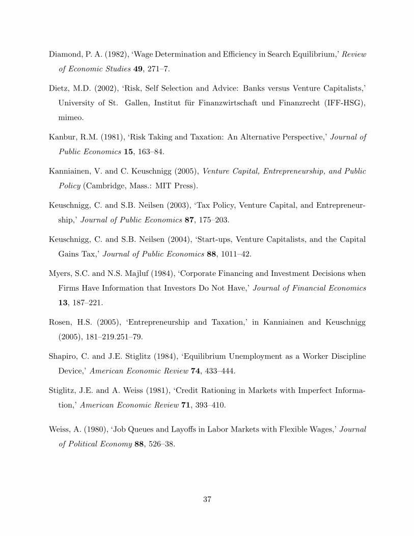
Diamond, P. A. (1982), ‘Wage Determination and Efficiency in Search Equilibrium,’ Review

of Economic Studies 49, 271–7.

Dietz, M.D. (2002), ‘Risk, Self Selection and Advice: Banks versus Venture Capitalists,’

University of St. Gallen, Institut fur Finanzwirtschaft und Finanzrecht (IFF-HSG),

mimeo.

Kanbur, R.M. (1981), ‘Risk Taking and Taxation: An Alternative Perspective,’ Journal of

Public Economics 15, 163–84.

Kanniainen, V. and C. Keuschnigg (2005), Venture Capital, Entrepreneurship, and Public

Policy (Cambridge, Mass.: MIT Press).

Keuschnigg, C. and S.B. Neilsen (2003), ‘Tax Policy, Venture Capital, and Entrepreneur-

ship,’ Journal of Public Economics 87, 175–203.

Keuschnigg, C. and S.B. Neilsen (2004), ‘Start-ups, Venture Capitalists, and the Capital

Gains Tax,’ Journal of Public Economics 88, 1011–42.

Myers, S.C. and N.S. Majluf (1984), ‘Corporate Financing and Investment Decisions when

Firms Have Information that Investors Do Not Have,’ Journal of Financial Economics

13, 187–221.

Rosen, H.S. (2005), ‘Entrepreneurship and Taxation,’ in Kanniainen and Keuschnigg

(2005), 181–219.251–79.

Shapiro, C. and J.E. Stiglitz (1984), ‘Equilibrium Unemployment as a Worker Discipline

Device,’ American Economic Review 74, 433–444.

Stiglitz, J.E. and A. Weiss (1981), ‘Credit Rationing in Markets with Imperfect Informa-

tion,’ American Economic Review 71, 393–410.

Weiss, A. (1980), ‘Job Queues and Layoffs in Labor Markets with Flexible Wages,’ Journal

of Political Economy 88, 526–38.

37

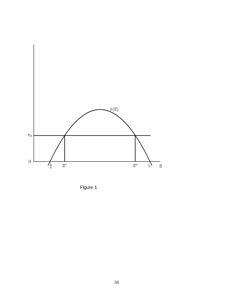
a

π0

12

01

π(a)

a∗ au

.................................................................................................................................................................................................................................................................................................................................................................................................................................................................................................................................................................................................................................................................................................................................................................................................................................................................................................................................................................................................................................................................................................................................................................................................................................................................................................................................

...............................

...............................

...............................

...............................

...............................

...............................

...............................

...............................

...............................

......

...............................

...............................

...............................

...............................

...............................

...............................

...............................

...............................

...............................

......

...................................................................................................................................................................................................................................................................................................................................................................................................................................................................................................................................................................

.......................................................................................................................................................

................................................................................................................................................................................................................................................................................................................................................................................................................................................................................................................................................................................................................................................................................................................................................................................................................................................................................................................................................................................................................................................................................................

Figure 1

38

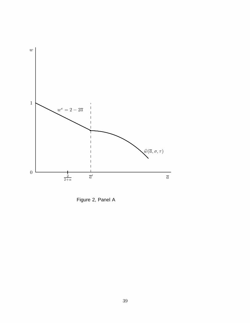
a

1

22+α

0

w

w(a, σ, τ)

we = 2 − 2a

a′

.............................................................................................................................................................................................................................................................................................................................................................................................................................................................................................................................................................................................................................................................

.............................

..........................................................................................................................................................................................................................................................................................................................................................................................................................................................................................................................................................................................................................................................................................................

........

.....

........

.....

........

.....

........

.....

........

.....

........

.....

........

.....

........

.....

........

.....

........

.....

........

.....

........

.....

........

.....

........

.....

......

Figure 2, Panel A

39

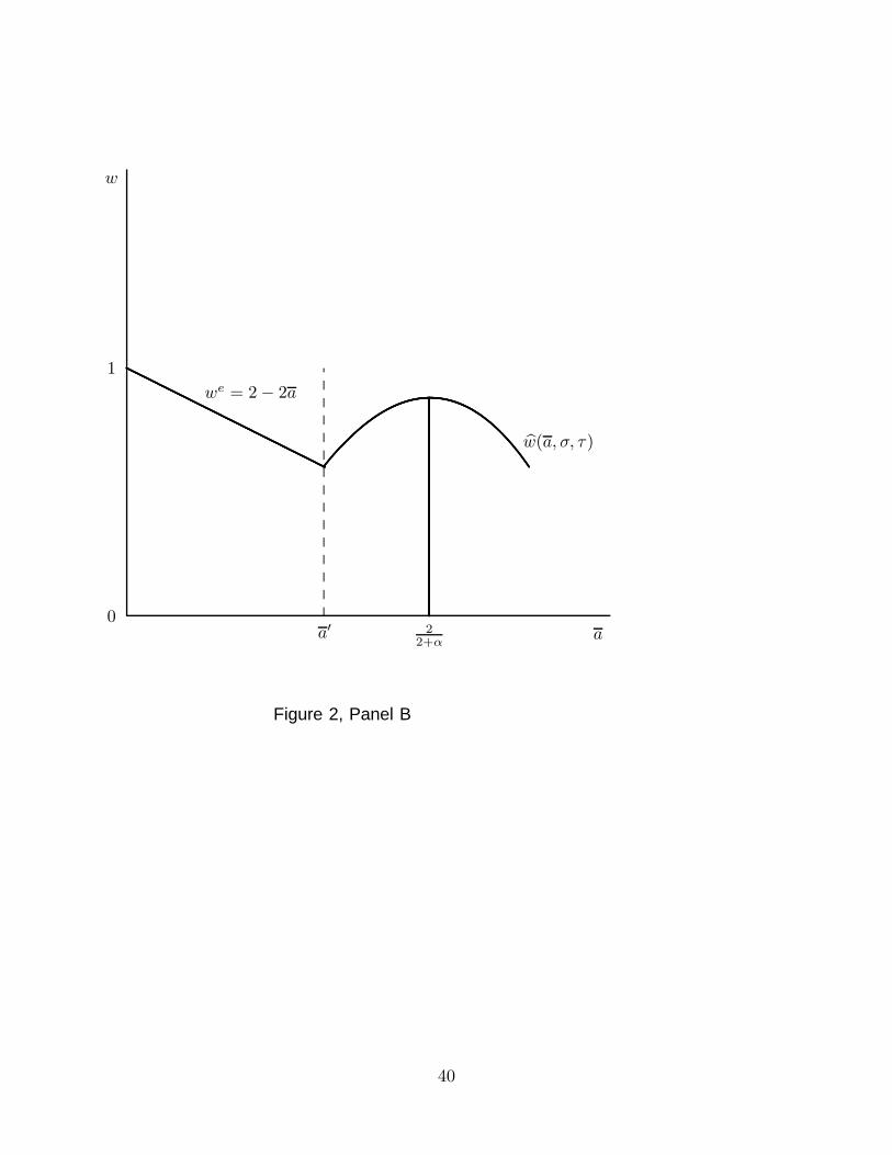
a

1

22+α

0

w

w(a, σ, τ)

we = 2 − 2a

a′

.............................................................................................................................................................................................................................................................................................................................................................................................................................................................................................................................................................................................................................................................

...............................

...............................

...............................

...............................

...............................

...............................

...............................

...............................

...............................

...............................

...............................

...............................

...............................

...............................

...............................

...............................

...............................

...............................

...............................

...............................

......

....................................................................................................................................................

....................................................................................................................................

...........................................................................................................................................................................................................................................................................................................................................................................................................................................................................

........

.....

........

.....

........

.....

........

.....

........

.....

........

.....

........

.....

........

.....

........

.....

........

.....

........

.....

........

.....

........

.....

........

.....

......

Figure 2, Panel B

40

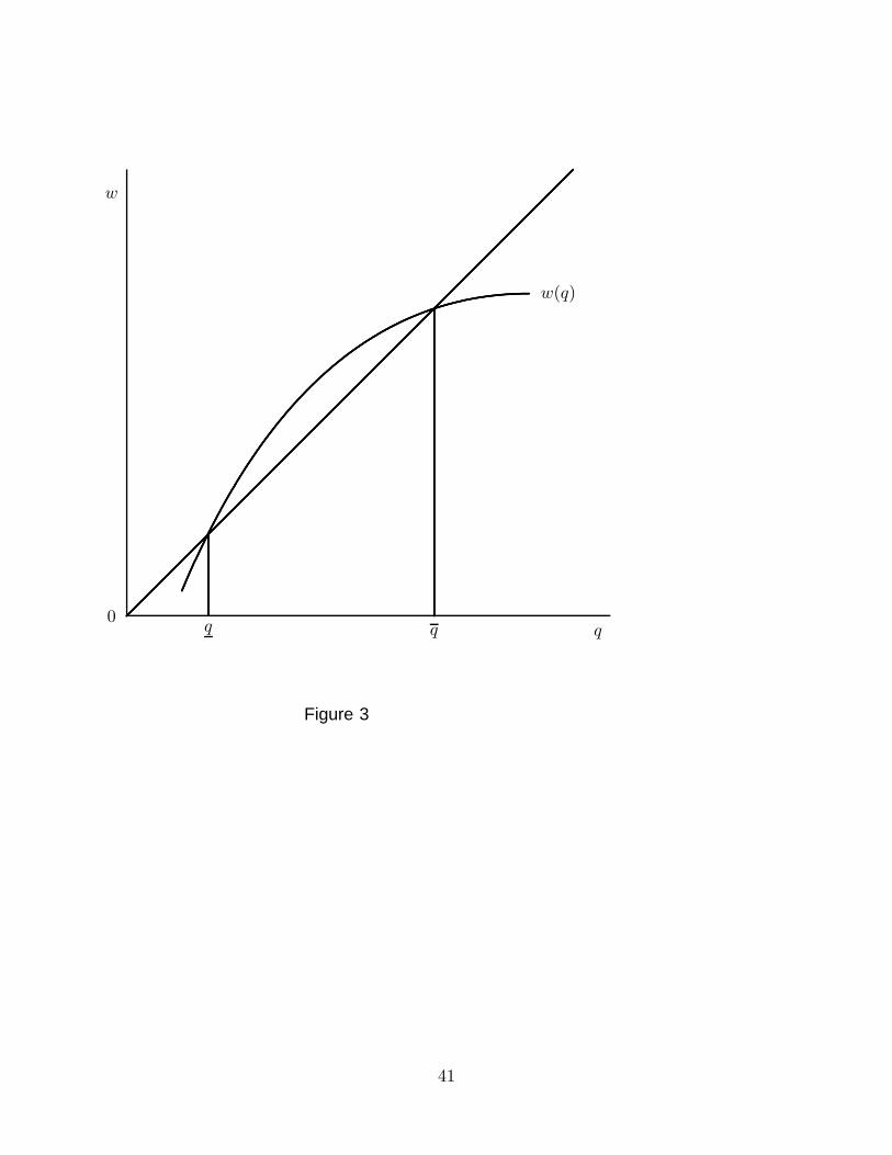
q

w

0q q

w(q)

...................................................................................................................................................................................................................................................................................................................................................................................................................................................................................................................................................................................................................................................................................................................................................................................................................................................................................................................................................................................................................................................................................................................................................................................................................................................................................................................................................................................................................................................................................................................................................................................................................................................................................................................................................................................................................................................................................

...............................

...............................

...............................

...............................

...............................

...............................

...............................

...............................

...............................

...............................

...............................

...............................

...............................

...............................

...............................

...............................

...............................

...............................

...............................

...............................

...............................

...............................

...............................

...............................

...............................

...............................

...............................

...............................

...............

...............................

...............................

...............................

...............................

...............................

...............................

...............................

..................

...................................................................................................................................................................................................................................................................................................................................................................................................................................................................................................................................................................................................................................................................................................................................................................................................................

..........................................................................................................

...............................................................................................................................

........................................................................................................................................................................................

..................................................................................................................................................................................................

Figure 3

41