Entrepreneurial Investment Dynamics And The WealthDistribution

Eugene Tan∗

This draft: Preliminary, Aug 2018.Click here for latest version

Abstract

This paper studies entrepreneurial investment behavior, and investigates the extentto which entrepreneurial risk taking contributes to wealth inequality. Using repre-sentative firm level data on startups, I find evidence that an entrepreneur’s capitalinvestment is illiquid. To quantify this, I construct an endogenous occupational choicemodel, where an entrepreneur holds two assets: liquid bonds and illiquid capital. Ifind that entrepreneurs lose about 68% to 79% of their investment when selling capital.Relative to a counter-factual economy where capital is fully liquid, high productiv-ity entrepreneurs operate smaller firms while low productivity entrepreneurs operatelarger firms; moreover, high productivity entrants delay entry, while low productivityentrepreneurs delay exit. This implies that capital is allocated towards low productivityentrepreneurs, and results in a higher population of wealthy but low productivity en-trepreneurs. Consequently, welfare and total factor productivity is substantially lowerrelative to the frictionless economy; moreover, fiscal policy that addresses capital illiq-uidity can considerably improve welfare. Finally, I find that the benchmark economyhas lower wealth inequality than the counter-factual economy, driven primarily by highproductivity entrepreneurs earning a lower ex-post return on their investment. Thisfinding suggests that macroeconomic models of entrepreneurship that ignore illiquiditymight over-state the contribution of entrepreneurial risk taking to the dispersion ofwealth in the data. (JEL D31, E21, E22, L26)

∗Duke University. email: eugene.tan@duke.edu. Acknowledgements: I am indebted to my advisors,Andrea Lanteri and Craig Burnside, for their tireless support and advice in writing this paper. I wouldalso like to thank the rest of my committee members Matthias Kehrig, Cosmin Ilut, and Kyle Jurado, aswell as the rest of the macroeconomics group at Duke for their helpful comments and advice. I have alsobenefited substantially from conversations with Sungki Hong, B. Ravikumar, Juan Sanchez, Daniel Xu andChen Yeh. I would also like to thank the participants at the Fall 2017 Midwest Macro conference, 2017 SEAconference, and the 2018 NASMES conference for helpful discussion and comments. In addition, I wouldlike to thank the St Louis Federal Reserve for hosting me during the writing of this paper. Finally, I wouldlike to thank the Kauffman Foundation for providing sponsorship to access the Kauffamn Firm Survey atthe NORC enclave. All errors are my own.

1

1 Introduction

Ownership of a business is highly correlated with being wealthy - a fact that has been welldocumented in the earlier literature1. However, the returns to entrepreneurship is much lesswell understood2. As such, the question of whether entry into entrepreneurship is the driverof heterogeneity in wealth accumulation, or whether the wealthy simply disproportionatelypursue entrepreneurship, remains an open question. The goal of this paper is to (a) pro-vide direct empirical evidence of entrepreneurial investment dynamics, (b) rationalize theirbehavior using a macroeconomic model of entrepreneurship, and (c) through the lens of themodel, discuss whether entrepreneurship is a key determinant in generating the large wealthdispersion in the real economy.

In this paper, I present two key observations of entrepreneurial investment dynamicsfrom the Kauffman Firm Survey (KFS), a representative panel survey of newly formed firms.Firstly, I find that the distribution of the rates of return to capital, as proxied by the (log)average revenue product of capital (henceforth just ARPK), of young entrepreneurial firms ishighly left skewed. Secondly, firms also exhibit large autocorrelation in ARPK, with greaterpersistence in the left tail of the cross-section distribution than the right.

Taken together, this suggests that the returns to entrepreneurship is generally very low;crucially, the downside risk can be much larger than the upside risk, as evinced by the leftskewness of the distribution. Moreover, entrepreneurs with low rates of return to capitalappear to persistently deliver low rates of return, and at a higher persistence than their highperforming counterparts.

The evidence runs counter to the current paradigm of entrepreneurial firm dynamics,which has focused largely on financial constraints driven by collateralized borrowing. Inthat framework, high productivity entrepreneurs face investment constraints, and thus oper-ate sub-optimally small firms relative to their productivity. This increases the population ofentrepreneurs with high returns to capital, generating a right-skewed distribution of returns.Moreover, as financially constrained entrepreneurs are also more likely to be constrainedfor several periods, this elevated returns to capital will persist for several periods. In con-trast, as entrepreneurs do not face downsizing frictions in that paradigm, poor performingentrepreneurs downsize within a period, reverting quickly back to the mean. Therefore, thecollateral constraints model predicts that the right tail is more persistent than the left, acounterfactual prediction given my findings3.

1c.f. Quadrini (1999), Cagetti and De Nardi (2006), Kuhn and Rios-Rull (2015)2For instance, there is still a debate regarding whether entrepreneurial undertaking has higher or lower

returns than labor work, c.f. Hamilton (2000), Manso (2015), Dillon and Stanton (2017)3The theoretical proof of this effect is provided in the appendix

2

In order to explain these findings, I construct a model that incorporates partial irre-versibility of entrepreneurial capital4. I build on the framework of Cagetti and De Nardi(2006), and extend their endogenous occupational choice incomplete markets model by dif-ferentiating between liquid assets (bonds) and illiquid assets (entrepreneur’s capital). Due toan asymmetry in the purchase and resale price of capital, rather than downsizing or exitinginstantly when hit by a bad shock, entrepreneurs adopt a “wait-and-see” attitude. This illiq-uidity effect, originating from a real options value effect, leads them to operate larger thanoptimal firm sizes5, generating a naturally left-skewed distribution of log ARPK. Moreover,this also creates persistence in the left tail as entrepreneurs wait out the transient bad shock.

To evaluate the quantitative significance of this friction, I calibrate the model to iden-tifying micro-level moments drawn from the KFS. I find that for every unit of capital sold,the entrepreneur loses 68% of the underlying real value of the capital asset. Upon exit, theentrepreneur faces an additional 31% write down on her assets6.

A direct consequence of these large downsizing frictions is capital and talent mis-allocationrelative to a counter-factual economy where capital is fully liquid. Along the intensivemargin, low productivity entrepreneurs operate larger firms while high productivity en-trepreneurs operate smaller firms; the latter effect arising due to a fall in the put optionvalue of capital. Along the extensive margin, high productivity entrants delay entry whilelow productivity incumbents delay exit. As a result, wealthier entrepreneurs have lower aver-age productivity, while poorer entrepreneurs have higher average productivity. This outcomeleads to substantial TFP and welfare loses relative to the counter-factual economy: Steadystate aggregate TFP is 11% higher, while average welfare, factoring transitional dynamics,is 4.4% higher in consumption equivalent terms.

In addition, capital illiquidity also magnifies the effect of un-insurable capital incomerisk, leading entrepreneurs to accumulate more liquid assets relative to the counter-factualeconomy7. Consequently, fiscal policy that provides consumption insurance against thisilliquidity risk can improve economic efficiency. For instance, I find that a policy thatdirectly increases the resale value of capital, funded by a proportional tax on bond returns,

4Partial irreversibility could arise naturally because the resale price of “used” capital is lower than thepurchase price of new capital, as discussed in Lanteri (2016)

5“Optimal" here refers to the case where the (expected) marginal product of capital is set equal to thesum of the interest rate and the user cost of capital.

6This is not the only source of friction in the model that makes entrepreneurial capital illiquid. To matchthe data, the model also includes a proportional investment fixed cost of about 3.4%. While these frictionsmight seem large, they are comparable to prior research in both the households (c.f. Diaz and Luengo-Prado(2010), Kaplan and Violante (2014) and Berger and Vavra (2014)) and firm dynamics (c.f. Cooper andHaltiwanger (2006), Bloom (2009), and Gilchrist et al (2014) literature.

7This effect is reminiscent of the question studied in Aiyagari (1994), where the author studies whetherprecautionary savings leads to savings in excess of the complete markets representative agent model.

3

can improve economic outcomes in terms of welfare and total factor productivity.The results have important implications for both the applied microeconomics and macroe-

conomics research on entrepreneurship. On the applied microeconomics front, recent researchhave exploited variations in asset prices (typically house prices) to test the presence of col-lateral constraints. A general strategy for this literature is to regress some macroeconomicoutcome (such as startup rates) on house price variations8, and attribute the correlation tocollateral constraints. In this paper, the illiquidity effect has qualitatively similar effects toa collateral constraint; for instance, negative shocks to the resale value of capital depressesentry due to a fall in the option value of capital (and hence entrepreneurship). Therefore, tothe extent that house or asset prices covary positively with resale capital prices, the resultsin the preceding literature might be contaminated by the illiquidity effect.

On the macroeconomics front, relative to a standard Aiyagari (1994) model of laborincome risk, entrepreneurship in a heterogeneous household model improves the model fit tothe top wealth shares of the US economy (the top 1%, 5% and 10%). However, the modelwealth distribution is more egalitarian than the real economy (Gini coefficient of about0.68; the data is about 0.8). This result arises because the illiquidity effect depresses theoverall returns to capital: The same effect that allows the model to capture the left skewnessof the ARPK distribution also generate substantial numbers of low returns entrepreneurs.As a consequence, wealth dispersion is lower in the benchmark economy. In contrast, acounterfactual “frictionless" economy has substantially higher wealth dispersion and matchesthe empirical wealth distribution closer; for instance, the Gini is about 0.76. This impliesthat macroeconomic models of entrepreneurship that ignore illiquidity will overstate thecontribution of entrepreneurship to wealth dispersion.

1.1 Related literature

This paper contributes to three main strands of the macroeconomics literature: Householddynamics, entrepreneur dynamics, and firm dynamics.

Household dynamics This paper is most related to the research agenda framed byQuadrini (2000) and Cagetti and De Nardi (2006), which study the contribution of en-trepreneurship to wealth inequality. In that framework, the entrepreneur’s business wealthand savings wealth are perfect substitutes. In this paper, I generalize their framework toone that distinguishes between business wealth and savings wealth. Business wealth (en-trepreneurial capital) is illiquid and subject to transaction costs. Unlike in Cagetti and

8See for example, Adelino et al (2015) or Schamlz et al (2017). Schott (2015) studies a similar mechanism,but explores it in a macroeconomic context.

4

De Nardi (2006), I find that entrepreneurial risk taking alone does not account for the fulldispersion of wealth; as capital is illiquid, overall returns to entrepreneurship are heavilydepressed, resulting in lower wealth dispersion compared to a frictionless economy.

I also add to that research agenda by contributing direct empirical evidence regardingthe investment behavior of entrepreneurs, and calibrating my model directly to data onentrepreneurs. In contrast, Quadrini (2000) and Cagetti and De Nardi (2006) calibrate theirmodel to match the income process of entrepreneurs identified from the Panel Survey ofIncome Dynamics (PSID) or Survey of Consumer Finances (SCF). In the latter strategy,one is generally unable to identify who constitutes entrepreneurs, as well as what portion ofthe entrepreneur’s income should be considered capital income, and what is consider laborincome. Moreover, the book value of capital is not available in household surveys, makingit difficult to assess the model’s ability in matching actual investment behavior.

In addition, this paper is connected to a growing literature on rates of returns heterogene-ity and its effect on the wealth distribution. Recent empirical work has showed that highlypersistent and heterogeneous returns to wealth can largely explain the income and wealth in-equality in the economy9, while recent theoretical work by Benhabib et al (2015) provide thetheoretical underpinning to explain why this particular mechanism is so successful in match-ing the wealth distribution. This paper adds to the literature that uses entrepreneurship asa micro-foundation to understand heterogeneity in rates of return among households.

More broadly speaking, this paper also adds to the growing literature on using quanti-tative heterogeneous agent macroeconomic models to understand the determinants of theempirical wealth distribution. This literature, dating back to Aiyagari (1994), has largelydocumented that a model of only exogenous labor income risk cannot, in general, match thewealth distribution without resorting to a largely counter-factual labor income process10.This paper adds to the research agenda of using entrepreneurship to augment the basicAiyagari model to understand wealth inequality.

Entrepreneur dynamics This paper is relevant to a broad range of research that studiesentrepreneurial investment dynamics and issues associated with it, such as capital taxation,estate taxation, or financial frictions11. This paper finds that the entrepreneur’s entry/exit

9c.f. Saez and Zucman (2014) for tax returns data from the United States, Bach et al (2016) for data onSweden, and Fagereng et al (2016) for data on Norway.

10See in particular Castaneda et al (2003) and Benhabib et al (2016) for discussions on how calibratedlabor income risk are typically counterfactual to the real amount of risk households face. Hurst et al (2010)also provides a discussion on the importance of directly modeling business ownership when studying thewealth distribution.

11For capital income taxation, see for instance Kitao (2008) and Panousi and Angeletos (2012); for estatetaxation, see for example Cagetti and De Nardi (2009); for financial frictions and collateral constraints, see

5

and investment decision in a two asset framework differs starkly from the one asset model.For instance, I find that the illiquidity effect endogenously induces entrepreneurs to runsmaller firms or delay entry. This replicates the effect of collateral constraints, but is auniquely different channel that cannot be addressed by fiscal policy targeted towards ad-dressing financing constraints. Moreover, this paper raises an identification challenge for theapplied microeconomics literature that relates financing constraints, via house price varia-tions, to macroeconomic outcomes through an entrepreneurship channel12. Taken together,this paper motivates the use of a liquid-illiquid asset framework for future research that isconcerned with understanding entrepreneurial investment dynamics.

Firm dynamics This paper relates to the broad literature that studies the relationshipbetween real and financial frictions and capital mis-allocation13. Here, I developed a simplediagnostic to disentangle financial frictions (driven by collateral constraints) and illiquidityeffects driven by partial irreversibility. Specifically, I show that the dynamic behavior of theARPK distribution is critical in helping distinguish between investment or disinvestmentfrictions. To the best of my knowledge, this is the first paper that has exploited this aspectof the ARPK distribution.

This paper also adds to that literature by providing a bridge between understanding thedispersion of wealth and the dispersion of marginal products of capital. In this paper, Iconnect the mis-allocation of capital back to the wealth distribution through the lens of aheterogeneous agents model that merges an incomplete markets model with a firm dynamicsmodel.

The rest of this paper is divided as follow. In section 2, I give a summary and descriptionof the data and stylized moments. Following that, in section 3, I describe the model, as wellas give a short discussion on why standard investment models are unable to explain thisdata. In section 4, I discuss in detail the calibration strategy; in particular, I explain howmy model can discriminate between illiquidity frictions and collateral constraints. Section5 discusses the model results of the calibration exercise. Section 6 extends the model tostudy the impact of illiquidity frictions on fiscal policy instruments and dynamic outcomes,and show why modeling illiquidity in this framework is important. Section 7 concludes thepaper.

for instance Evans and Jovanovic (1989), Buera et al (2011), Buera and Shin (2013), Adelino et al (2015),Bassetto et al (2015).

12See for instance, Adelino et al (2015) and Schmalz et al (2017).13See for instance, Beura et al (2011), Buera and Shin (2013), Asker et al (2014), Midrigan and Xu (2014).

6

2 Stylized Facts

In this section, I first briefly describe the data source. I then report the stylized facts re-garding entrepreneurial investment, focusing specifically on the distribution and dynamicbehavior of the average revenue of product of capital and investment rates. The data con-struction is relegated to the appendix.

2.1 Data universe

The data is drawn primarily from the restricted version of the Kauffman Firm Survey (KFS).The KFS is a single cohort panel survey, consisting solely of entrepreneurial firms that wereformed in the year 2004, and tracked through 2011. The universe of firms considered forsurvey inclusion was all newly registered firms in 2004 from the Dun and Bradstreet database.The subset of firms in this universe that was included in the survey must then satisfy thefollowing conditions:

1. Business was started as independent business, or by the purchase of an existing busi-ness, or by the purchase of a franchise in the 2004 calendar year.

2. Business was not started as a branch or a subsidiary owned by an existing business,that was inherited, or that was created as a not-for-profit organization in the 2004calendar year.

3. Business had a valid business legal status (sole proprietorship, limited liability com-pany, subchapter S corporation, C-corporation, general partnership, or limited part-nership) in 2004.

4. Business reported at least one of the following activities:

(a) Acquired employer identification number during the 2004 calendar year

(b) Organized as sole proprietorships, reporting that 2004 was the first year they usedSchedule C or Schedule C-EZ to report business income on a personal income taxreturn

(c) Reported that 2004 was the first year they made state unemployment insurancepayments

(d) Reported that 2004 was the first year they made federal insurance contributionact payments

7

As one can observe, the inclusion criterion is very strict, and relates largely to the commonidea of an entrepreneur. For a more complete description of the broad characteristics of thedata, especially on the firm’s balance sheet, I refer the reader to Robb and Robinson (2014).

A big advantage of utilizing the KFS in this paper is the ability to directly observethe investment dynamics of new and privately-owned firms (via the balance sheet of thefirm). As a result, the findings in the KFS can be directly mapped into a model that jointlydescribes heterogeneous household and firm dynamics. In contrast, the prior literature thathas studied entrepreneurial investment dynamics has utilized either household surveys suchas the Panel Survey of Income Dynamics (PSID), or datasets comprising large firms (suchas Compustat).

Both methods have several disadvantages relative to the KFS for understanding en-trepreneurship and its relation to the wealth distribution. In the context of householdsurveys, important information on the returns on firm assets, such as the marginal productof capital, is not computable as households do not report the book value of the firm’s asset14.Moreover, the sample has substantial attrition. As a result, it is difficult to draw substantiveinference on the dynamics of capital accumulation (or de-cumulation), which requires a longpanel survey.

For the literature that uses datasets on large firms, the nature of large firms mean thatit is generally possible for the primary owner or manager to fully diversify the idiosyncraticrisks of the firm. As a result, observations drawn from this data is not directly applicableto research on new firms. Moreover, this makes data on large firms an inappropriate datasource for a incomplete markets household model, which is a necessary model primitive forunderstanding the wealth distribution.

Finally, there is also a small but growing literature that uses Census micro-data to studynew firm behavior 15. Unfortunately, the census micro-data in general does not provide muchinformation on the balance sheet of private firms. As a result, while it is possible to matcha primary owner to her/his firm, we are not able to study the return on firm assets usingthese data sets.

14The PSID typically asks the households for their perceived value of their firm. A typical question, suchas the 2013 wave, asks respondents the following: “How much is your part of the business worth, that is,how much would it sell for".

15for instance, the Longitudinal Business Database (LBD) or the Longitudinal Employer-Household Dy-namics (LEHD)

8

2.2 Distribution and Dynamics of the Average Revenue Product of

Capital

(a) Distribution of log ARPK.

(b) Local polynomial fit of log ARPK at timet v.s log ARPK at time t− 1. The two verticallines are reference lines for the first and fifthquintile of the cross-sectional distribution.

(c) Local polynomial fit of the first difference of logARPK at time t vs time log ARPK at time t − 1.The two vertical lines are reference lines for the firstand fifth quintile of the cross-sectional distribution.

Figure 1: Top: The cross-sectional distribution of log ARPK. Bottom: The dynamics of logARPK.

2.2.1 Cross-sectional moments

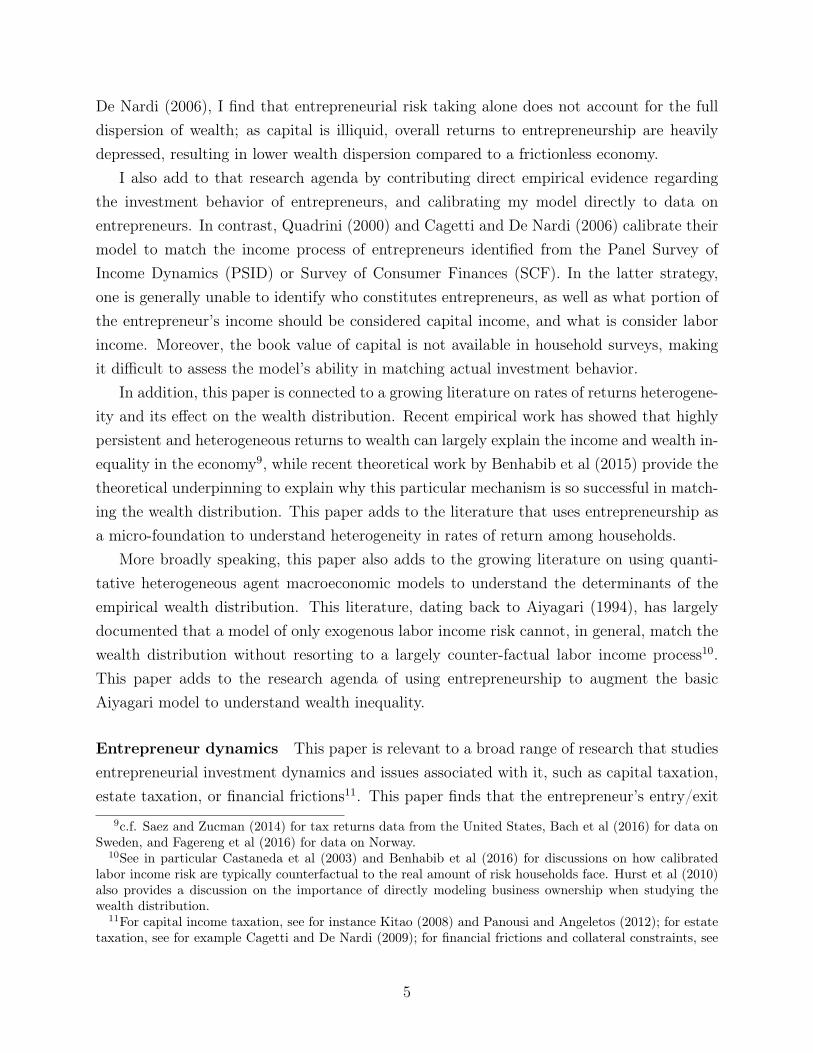
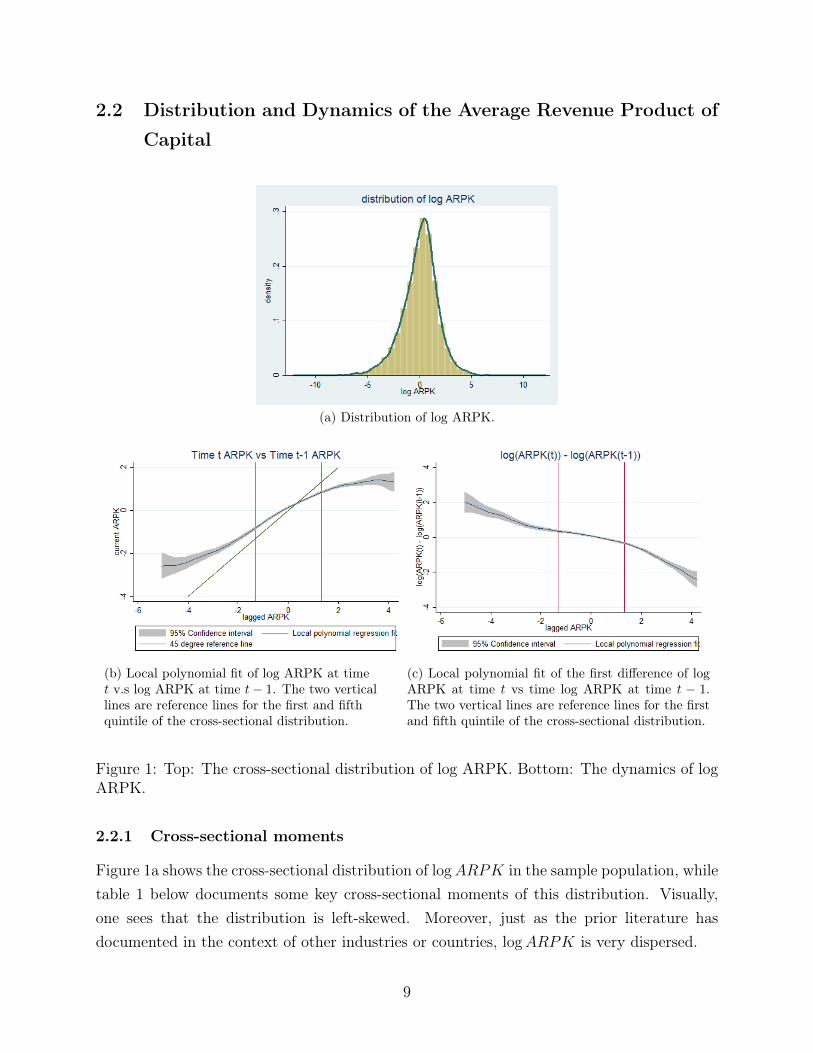
Figure 1a shows the cross-sectional distribution of logARPK in the sample population, whiletable 1 below documents some key cross-sectional moments of this distribution. Visually,one sees that the distribution is left-skewed. Moreover, just as the prior literature hasdocumented in the context of other industries or countries, logARPK is very dispersed.

9

Mean Standard Deviation Skewness Kurtosis0.00 1.75 -0.39 5.7

Table 1: Selected moments from distribution of logARPK

2.2.2 Dynamics of logARPK

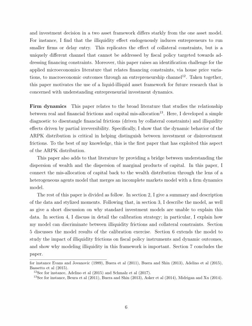
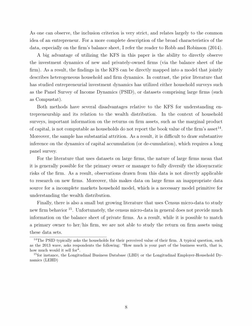
Figure 1b plots a local polynomial fit of the current period log ARPK against the last periodlog ARPK. A 45◦ reference line is overlaid on the plot. Figure 1c plots a local polynomialfit of the first difference of log ARPK (i.e. logARPKt − logARPKt−1) against last periodlog ARPK.

What do these two graphs tell us about the dynamics of the average revenue productof capital? Note that if ARPK is perfectly persistent, then all the data points should lineup on the 45◦ line in figure 1b; along a similar vein, figure 1c would reflect a flat horizontalline at 0. In contrast, if ARPK was i.i.d.. then the local polynomial fit in figure 1b wouldfeature a flat horizontal line at 0. As we can see from the graphs, ARPK is highly persistentin the sample, but there is still some significant churning.

We can also tell from these graphs that this persistence is asymmetric, being greater onthe left tail than the right. For instance, looking at figure 1b, a firm that starts out withlogARPK = −4 (i.e. in the left tail) will, on average, end up with logARPK ≈ −2.5 in thenext period (equivalent, the difference would be about 1.5, when view from the perspectiveof figure 1c). In contrast, a firm that starts out with logARPK = 4 will end up, on average,with logARPK ≈ −1.5 in the next period.

To quantify this asymmetry, I document this fact in two ways: (1) By estimating atransition matrix for logARPK, and (2) by estimating the conditional autocorrelation oflogARPK.

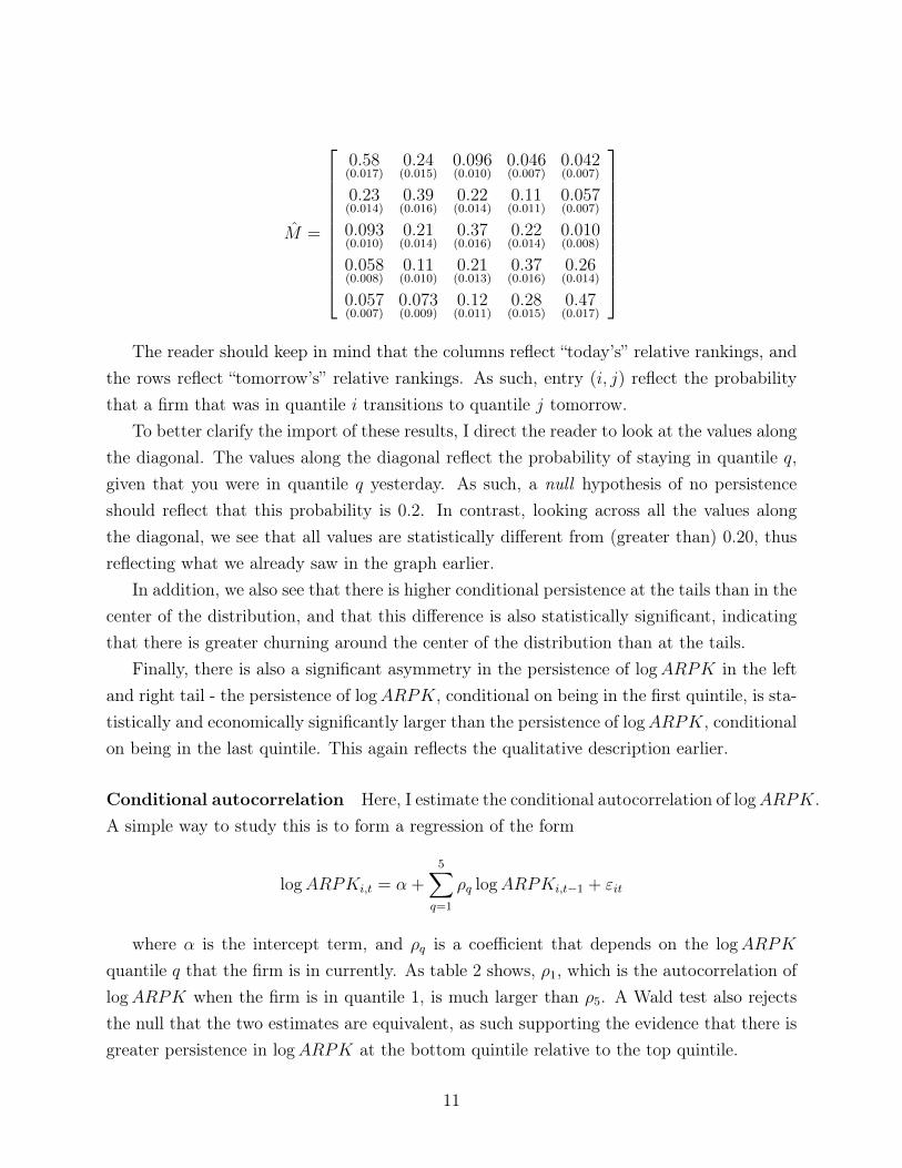
Transition matrix Here, I estimate the persistence in relative rankings by first binningthe firms into quintiles (estimated at the industry level) on a year-by-year basis16, and thenestimating the transition matrix M (across quintiles) for the entire sample. I report theestimated transition matrix below, with standard errors in parenthesis below the estimatedvalue:

16I have also estimated the transition matrix by fixing the quintiles to the bins in 2004. The results arevery similar. Refer to the appendix for additional robustness checks.

10

M =

0.58(0.017)

0.24(0.015)

0.096(0.010)

0.046(0.007)

0.042(0.007)

0.23(0.014)

0.39(0.016)

0.22(0.014)

0.11(0.011)

0.057(0.007)

0.093(0.010)

0.21(0.014)

0.37(0.016)

0.22(0.014)

0.010(0.008)

0.058(0.008)

0.11(0.010)

0.21(0.013)

0.37(0.016)

0.26(0.014)

0.057(0.007)

0.073(0.009)

0.12(0.011)

0.28(0.015)

0.47(0.017)

The reader should keep in mind that the columns reflect “today’s” relative rankings, and

the rows reflect “tomorrow’s” relative rankings. As such, entry (i, j) reflect the probabilitythat a firm that was in quantile i transitions to quantile j tomorrow.

To better clarify the import of these results, I direct the reader to look at the values alongthe diagonal. The values along the diagonal reflect the probability of staying in quantile q,given that you were in quantile q yesterday. As such, a null hypothesis of no persistenceshould reflect that this probability is 0.2. In contrast, looking across all the values alongthe diagonal, we see that all values are statistically different from (greater than) 0.20, thusreflecting what we already saw in the graph earlier.

In addition, we also see that there is higher conditional persistence at the tails than in thecenter of the distribution, and that this difference is also statistically significant, indicatingthat there is greater churning around the center of the distribution than at the tails.

Finally, there is also a significant asymmetry in the persistence of logARPK in the leftand right tail - the persistence of logARPK, conditional on being in the first quintile, is sta-tistically and economically significantly larger than the persistence of logARPK, conditionalon being in the last quintile. This again reflects the qualitative description earlier.

Conditional autocorrelation Here, I estimate the conditional autocorrelation of logARPK.A simple way to study this is to form a regression of the form

logARPKi,t = α +5∑q=1

ρq logARPKi,t−1 + εit

where α is the intercept term, and ρq is a coefficient that depends on the logARPK

quantile q that the firm is in currently. As table 2 shows, ρ1, which is the autocorrelation oflogARPK when the firm is in quantile 1, is much larger than ρ5. A Wald test also rejectsthe null that the two estimates are equivalent, as such supporting the evidence that there isgreater persistence in logARPK at the bottom quintile relative to the top quintile.

11

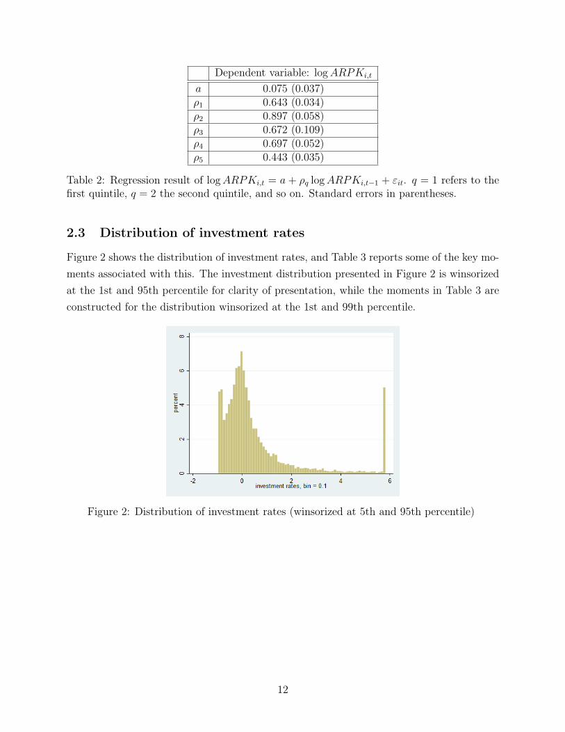
Dependent variable: logARPKi,t

a 0.075 (0.037)ρ1 0.643 (0.034)ρ2 0.897 (0.058)ρ3 0.672 (0.109)ρ4 0.697 (0.052)ρ5 0.443 (0.035)

Table 2: Regression result of logARPKi,t = a + ρq logARPKi,t−1 + εit. q = 1 refers to thefirst quintile, q = 2 the second quintile, and so on. Standard errors in parentheses.

2.3 Distribution of investment rates

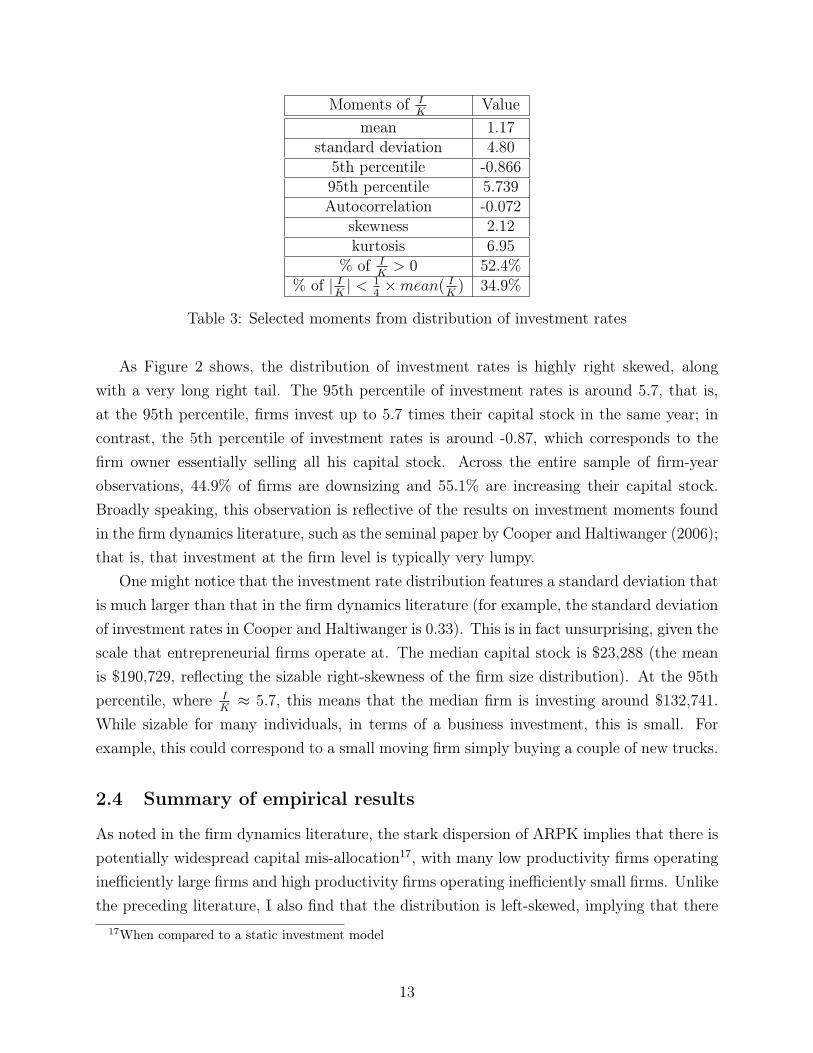
Figure 2 shows the distribution of investment rates, and Table 3 reports some of the key mo-ments associated with this. The investment distribution presented in Figure 2 is winsorizedat the 1st and 95th percentile for clarity of presentation, while the moments in Table 3 areconstructed for the distribution winsorized at the 1st and 99th percentile.

Figure 2: Distribution of investment rates (winsorized at 5th and 95th percentile)

12

Moments of IK

Valuemean 1.17

standard deviation 4.805th percentile -0.86695th percentile 5.739Autocorrelation -0.072

skewness 2.12kurtosis 6.95

% of IK> 0 52.4%

% of | IK| < 1

4×mean( I

K) 34.9%

Table 3: Selected moments from distribution of investment rates

As Figure 2 shows, the distribution of investment rates is highly right skewed, alongwith a very long right tail. The 95th percentile of investment rates is around 5.7, that is,at the 95th percentile, firms invest up to 5.7 times their capital stock in the same year; incontrast, the 5th percentile of investment rates is around -0.87, which corresponds to thefirm owner essentially selling all his capital stock. Across the entire sample of firm-yearobservations, 44.9% of firms are downsizing and 55.1% are increasing their capital stock.Broadly speaking, this observation is reflective of the results on investment moments foundin the firm dynamics literature, such as the seminal paper by Cooper and Haltiwanger (2006);that is, that investment at the firm level is typically very lumpy.

One might notice that the investment rate distribution features a standard deviation thatis much larger than that in the firm dynamics literature (for example, the standard deviationof investment rates in Cooper and Haltiwanger is 0.33). This is in fact unsurprising, given thescale that entrepreneurial firms operate at. The median capital stock is $23,288 (the meanis $190,729, reflecting the sizable right-skewness of the firm size distribution). At the 95thpercentile, where I

K≈ 5.7, this means that the median firm is investing around $132,741.

While sizable for many individuals, in terms of a business investment, this is small. Forexample, this could correspond to a small moving firm simply buying a couple of new trucks.

2.4 Summary of empirical results

As noted in the firm dynamics literature, the stark dispersion of ARPK implies that there ispotentially widespread capital mis-allocation17, with many low productivity firms operatinginefficiently large firms and high productivity firms operating inefficiently small firms. Unlikethe preceding literature, I also find that the distribution is left-skewed, implying that there

17When compared to a static investment model

13

might be substantially more firms that are large with low productivity, than small firms withhigh productivity. Moreover, the asymmetric persistence implies that the former operate atthis inefficient level for longer periods of time than the latter, which then naturally givesrise to the left skewed cross-sectional distribution. This suggests that entrepreneurial firmsare facing frictions in both capital accumulation and decumulation, but the latter frictionappears to be stronger.

In addition, the investment distribution reveals that entrepreneurial firm investment islumpy and infrequent, which suggests that non-convex adjustment costs play a potentiallyhuge role in influencing entrepreneurial firm investment behavior.

Taken as a whole, the results are suggestive that partial irreversibility of capital, whichinduces an asymmetry in the purchase and resale value of capital, could rationalize thedynamic investment behavior observed here18. In particular, partial irreversibility, whenmodeled as a proportional transaction cost, induces the (s,S) investment dynamics that iscrucial in generating lumpy (dis)-investment. The lower resale value of used capital alsoinduces entrepreneurs to adopt a wait-and-see attitude when a bad shock is realized, thusoperating firms that are “too large" relative to their productivity. This leads to an elongatedleft tail of ARPK, generating a left skewness in the distribution of ARPK. In addition,this also leads to greater persistence in the left tail. These heuristics therefore provide themotivation to include partial irreversibility as a key mechanism in the model, which I discussin the following section.

3 Model

3.1 Households, occupation, and wealth

There is a continuum of mass 0 households in this economy, each indexed by i ∈ [0, 1].Households are infinitely lived, and time is discrete.

All households are endowed with identical time-separable utility function with constantrelative risk aversion (CRRA), and discount future utility at rate β. Households value aconsumption bundle c, which is the sum of non-durable consumption c and (non-market)home production output c. c is an endowment that is constant across time and households,whereas c depends on the household’s endowment of other factors and savings choices.

18See for example, Cabellero (1999) for a summary of models with partial irreversibility

14

Taken together, the household’s lifetime expected utility can be written as

V0 ≡ E0

∞∑t=0

βtU (ci,t)

= E0

∞∑t=0

βtc1−γi,t

1− γ

ci,t = ci,t + c

where γ is the coefficient of relative risk aversion. The household’s objective is to maxi-mize expected lifetime utility.

There are two types of occupations available to the households: To become an en-trepreneur, or to become a worker. The key distinction between entrepreneurs and workerslie in their endowments, their way of generating income, and their way of accumulatingwealth. The latter sections provide a more detailed description, but I briefly summarize thekey differences between entrepreneurs and workers here:

Endowments Entrepreneurs receive a stochastic endowment of a private business produc-tivity draw z ∈ Z, while worker’s receive a labor efficiency draw θ ∈ Θ. This productivitydraw is exclusive. Workers also receive a stochastic signal of business prospects ψz. ψz

informs the worker about the potential business prospects that she could engage in if sheswitches to becoming a business owner. Entrepreneurs receive a stochastic signal of laborprospects ψθ. ψθ informs the entrepreneur about the potential labor prospects that she couldengage in if she switches to becoming a worker.

Wealth Entrepreneurs accumulate two forms of wealth: illiquid physical capital k (whichthey use in production), and liquid bonds b, which pay off a fixed interest rate. Workers canonly save in liquid bonds. Physical capital is illiquid, as adjustment of the capital stock willlead the owner to incur specific adjustment costs (to be detailed later).

Technology All households are endowed with a fixed amount of labor supply l. Work-ers can combine their labor supply endowment with their labor productivity to produceeffective labor θl. They supply effective labor to a centralized labor market, and earn thecorresponding market wage w, giving them an income of wθl. Entrepreneurs have accessto a production function f (z, k, l), which allows them to combine illiquid capital k, laborl (including a fraction ι of their labor supply endowment), and business productivity z toproduce a consumption good ye which they sell into a centralized market for income.

15

3.2 Sources of uncertainty and occupational choice

3.2.1 Sources of uncertainty

There are four sources of idiosyncratic (and uninsurable) uncertainty in this economy. Theyare:

1. A stochastic Markov process Pz|z−1 ≡ Pr (z|z−1) over private business productivity,with support z ∈ Z and invariant distribution Fz.

2. A stochastic Markov process Pθ|θ−1 ≡ Pr (θ|θ−1) over labor productivity, with supportθ ∈ Θ and invariant distribution Fθ.

3. An IID process of signals regarding business prospects, with support ψz ∈ Ψz, anddistribution Fψz . Conditional on drawing a signal ψz, next period private business pro-ductivity is assumed to be drawn from the conditional probability Pz|ψz−1

≡ Pr(z|ψz−1

).

4. An IID process of signals regarding labor prospects, with support ψθ ∈ Ψθ, and dis-tribution Fψθ . Conditional on drawing a signal ψθ, next period labor productivity isassumed to be drawn from the conditional probability Pθ|ψθ−1

≡ Pr(θ|ψθ−1

).

3.2.2 Occupational choice

The occupation of the households determine the types of uncertainty they face. Specifically,as described earlier, only entrepreneurs receive endowments of business productivity andlabor prospect signal draws, and only workers receive endowments of labor productivity andbusiness prospect signal draws.

Households are allowed to endogenously choose their occupation, but they have to selecttheir occupation one period in advanced. In other words, a worker today who chooses to staya worker tomorrow must pursue his chosen occupation for the next period. Occupationalchoice is exclusive, so a household cannot be both a worker and an entrepreneur simultane-ously. This combination of “time-to-build” and exclusivity makes occupational choice itselfrisky.

Since there is endogenous occupational choice, we can in fact group the households intofour types. The exact classification of the household is important, as this determines thesources of uncertainty that they face. Specifically, we have the following:

1. Entrant entrepreneurs. Entrants entrepreneurs are entrepreneurs who were workerslast period. They are endowed with a productivity z that is drawn from the condi-tional distribution Pz|ψz−1

, where ψz−1 is the signal that the entrants had received in the

16

last period (as workers). They also receive a signal ψθ regarding next period’s laborprospects.

2. Incumbent entrepreneurs. Incumbents entrepreneurs are entrepreneurs who were en-trepreneurs last period. They are endowed with a productivity z that is drawn fromthe conditional distribution Pz (z|z−1), where z−1 is last period productivity that theyreceived as entrepreneurs. Like entrant entrepreneurs, they also receive a signal ψθ

regarding next period’s labor prospects.

Upon drawing ψθ, if the entrepreneur chooses to exercise this option and becomes aworker, her next period labor productivity follows the same Markov process as theworker. Otherwise, she loses the signal and draws a fresh signal next period from theinvariant distribution of signals.

3. Entrant workers. Entrants workers are workers who were entrepreneurs last period.They are endowed with a productivity θ that is drawn from the conditional distributionPθ|ψθ−1

. In addition, they receive a signal ψz regarding next period’s business prospects.

4. Incumbent workers. Incumbents workers are workers who were workers last period.They are endowed with labor productivity θ that is drawn from the conditional dis-tribution Pθ (θ|θ−1), where θ−1 is last period labor productivity that they received asworkers. Like entrant workers, they also receive a signal ψz regarding next period’sbusiness prospects.

Upon drawing ψz, if the worker chooses to exercise this option and starts a business, hernext period labor productivity follows the same Markov process as the entrepreneurs.Otherwise, she loses the signal and draws a fresh signal next period from the invariantdistribution of signals.

3.3 Asset structure

Households have access to 2 types of assets to smooth inter-temporal consumption: Liquidbonds b and illiquid physical capital k.

3.3.1 Entrepreneurial physical capital

Only households who elect to become (or stay) entrepreneurs tomorrow can save in illiquidphysical capital k. The primary purpose of the physical capital is as input for entrepreneurialproduction. However, it also serves a secondary purpose as consumption insurance. In

17

particular, entrepreneurs can use the illiquid asset to smooth consumption by selling offparts of his asset stock in bad times, or to use it as collateral to borrow for consumption.

Capital is illiquid because of frictions associated with adjusting the capital stock. Here,I assume 4 forms of frictions.

The first friction affects investment. Entrepreneurs who choose to increase their cap-ital stock face a proportional fixed adjustment cost fsk. The fixed cost parametrizes thedisruptions associated with expansion.

Two frictions influence the entrepreneur’s disinvestment decision. If the adjustment issmall, the entrepreneur pays a per-unit transaction cost λ, such that she recoups (1 − λ)

of the transacted asset. If the adjustment is large, she has to pay another proportionalselling cost ζ on top of the earlier transaction cost. As a result, the net return from sellinga unit of capital is (1 − ζ)(1 − λ). An adjustment is considered small if the volume ofdisinvestment ik is less than a fraction η ∈ [0, 1] of the entrepreneur’s depreciated capitalstock (i.e. ik ≤ η(1− δ)k)).

This preceding formulation imposes that small adjustments are more costly than largechanges, and captures the idea that large scale sales are akin to a “fire sale" of assets. Thisalso simultaneously parameterizes the difficulty of exiting a business and having to conducta fire sale of all the physical capital stock.19 In particular, η = 0 corresponds to a case whereonly exiting entrepreneurs are affected by this cost, whereas η = 1 captures a case where allentrepreneurs are affected.

Finally, the last friction involves entry. Specifically, it is assumed that workers who wantto enter entrepreneurship must start their business with a minimum level of capital kwmin.Households who are already entrepreneurs do not face this friction. Rather, this assumptionreflects the fact that entry typically requires some form of minimum capital investment.

3.3.2 Liquid bonds

All households can trade in bonds, either by buying bonds (i.e. saving), or selling them(i.e. borrowing). The total volume of bonds supplied composed of all the bonds issued byindividual households, as well as equity issued by a corporate sector. The cost of a bondthat pays off next period is 1 unit of consumption.

All bonds, regardless of whether it was issued by the corporate sector or individuals, pay19It is important to note that this does not necessarily say that every entrepreneur who exits a business

has to incur a loss. Rather, it says that when an entrepreneur exists his business, the physical capital stockthat he owns is typically worth less than even the actual depreciated value. On the other hand, this paperhas nothing to say about the potential profits to be made on intangible capital, such as brand name or R&Dcapital. I refer the reader to an accompanying paper in Tan (2018), where I extend this model frameworkto allow entrepreneurs to sell the business itself.

18

off the same interest rate r. As the corporate sector is large and is in fact issuing claimsagainst its profits, I assume that there is no spread between the cost at which the corporatesector borrows, and the interest rate received by savers. In contrast, individuals issuingbonds are essentially issuing unsecured debt, and hence are “riskier”. As such, I assume thatthe household must pay a per unit intermediation cost φd when they borrow. As a result,this induces a spread between the interest rate r received by savers, and interest rate rd paidby borrowers, given by rd = r + φd.

In addition, households who decide to invest in physical capital can also elect to use theliquid value of their physical capital as collateral to borrow in bonds. Specifically, I definethe liquid value of capital as (1− λ) (1− δ) k, and the collateral constraint is defined as

b′ ≥ −ϕ (1− λ) (1− δ) k′ − b

where ϕ ∈ [0,∞) , with ϕ = 0 representing no collateralized borrowing, and ϕ → ∞representing no collateral required for borrowing. Households are allowed to borrow up tothe liquid value of depreciated capital. b represents an ad-hoc borrowing constraint thatdoes not require any collateral. This reflects the nature that some households can acquireunsecured debt. As such, both workers and entrepreneurs can potentially borrow to smoothconsumption. The only difference is that entrepreneurs can borrow more.

Default Depending on the exact parametrization of the stochastic productivity process, asubset of entrepreneurs might not be able to fully pay off their stock of debt even after fullyliquidating. For this subset, the entrepreneurs are allowed to default on the remaining stockof their debt, but have to exit the entrepreneurial sector. The cost of default D (i.e. all thedebt that is unpaid) is transferred in a lump sum manner in equal proportions to the rest ofthe households20.

3.4 Sectors of the economy

There are two sectors of production in this economy: a corporate sector and an entrepreneurialsector. Both sector produce a single homogeneous non-durable consumption good.

3.4.1 Corporate sector

I assume that there exist a large corporate sector encompassing all non-entrepreneurial firms.This corporate sector is represented by a representative firm, which owns physical capital Kc

20In general, default does not occur in equilibrium in this model under the benchmark calibration. However,when studying unexpected shocks, fully leveraged households might find themselves unexpectedly in default.

19

and hires labor Lc from a centralized labor market. It has access to a standard Cobb-Douglasproduction technology of the form

Y c = A (Kc)α (Lc)1−α

where A is aggregate TFP, and α is the capital share. All households purchase equity incorporate firms, and are paid a dividend each period.

The corporate firm decides independently on how much physical capital to invest, andhow much labor to hire at the prevailing wage w. As such, the representative firm solves thestandard recursive problem

Π (K) = maxK′

π +1

1 + rΠ (K ′)

s.t.

π = Y c −(Kc′ − (1− δ)Kc

)− wLc

where π represents dividends paid out to the firms’ investors, and the firm discountsfuture profits at rate 1

1+r. Note that because of the size of the corporate sector, I assume

here that there are no adjustment costs associated with the corporate sector. Moreover,unlike entrepreneurs, corporate firms are allowed to issue equity, which is in line with thereal world observation of larger corporate firms being listed on a stock market. This marketarrangement leads to the standard first order condition

r + δ = αA

(Kc

Lc

)α−1

w = (1− α)A

(Kc

Lc

)α

3.4.2 Entrepreneurial sector

The entrepreneurial sector is composed of entrepreneurial households. They utilize the pro-duction function ye = f (z, k, l) = z (kαel1−αe)

ν . As discussed earlier, the inputs to produc-tion are physical capital k and labor l. ν ∈ (0, 1) here denotes the span-of-control, capturingthe fact that managerial skills become stretched over larger and larger projects.

Physical capital stock is chosen last period, and cannot be altered in the current period. z,as discussed earlier, is stochastic productivity and realized in the same period. Entrepreneursare endowed with labor supply l, and they can use a fixed fraction ι to run their own business.If they choose to hire extra workers, they have to pay the prevailing market wage w. As

20

such, the profit of the entrepreneurial firm can be written as

π (z, k) = z(kαel1−αe

)ν − w (l − ιl)Note that given this setup, the labor choice is a static decision and completely indepen-

dent of the structure of the rest of the problem. Consequently, we see that optimal labordemand satisfies:

l∗ =

ιl if l∗ ≤ ιl[(1−α)νw

] 11−(1−α)ν

z1

1−(1−α)ν kαν

1−(1−α)ν if l∗ > ιl

and optimal profits is given by

π∗ =

z(kα(ιl)1−α

)νif l∗ ≤ ιl[

A (w)− wA (w)1

(1−α)ν

]zΘzkΘk + wl if l∗ > ιl

where A(w) ≡[

(1−α)νw

] (1−α)ν1−(1−α)ν , Θz ≡ 1

1−(1−α)νand Θk ≡ αν

1−(1−α)ν.

3.5 Recursive formulation of the problem

The preceding problem can be recast compactly into recursive formulation. Denote by Veand Vw the value functions of entrepreneurs and workers respectively, by C (k′, k, h′, h) theadjustment cost function as described earlier, and h the occupational state (with 1 denotingworker and 0 denoting entrepreneur). Denote by ′ variables all next-period variables, andunprimed variables current variables. Given this, we have the following problem:

For entrepreneurs,

21

Ve(ψθ, z, k, b

)= max

h′,k′,b′,lU (c)

+ (1− h′)× β∫ψ′θ

∫z′Ve

(ψθ′, z′, k′, b′

)dPz′|zdFψθ

+ h′ × β∫ψ′z

∫θ′Vw

(ψz′, θ′, b′

)dPθ′|ψθdFψz

s.t.

π ≡ zf(k, ιl + l

)− wl +

(1 + r × 1{b≥0} + rd × 1{b<0}

)b− C (k′, k, h′, h)−D

c = max {π, 0} − k′ − b′ ≥ 0

k′

> 0 if h′ = 0

= 0 if h′ = 1

h′ = 1 ( if π < 0)

b′ ≥ −ϕ (1− λ) (1− δ) k′ − b

c = c+ c

For workers,

Vw (ψz, θ, b) = maxh′,k′,b′

U (c)

+ (1− h′)× β∫ψ′θ

∫z′Ve

(ψθ′, z′, k′, b′

)dPz′|ψzdFψθ

+ h′ × β∫ψ′z

∫θ′∈Θ

Vw

(ψz′, θ′, b′

)dPθ′|θdFψz

s.t.

c = θwl +(1 + r × 1{b≥0} + rd × 1{b<0}

)b− k′ − b′ −D

k′

> 0 if h′ = 0

= 0 if h′ = 1

b′ ≥ −ϕ (1− λ) (1− δ) k′ − b

c = c+ c

3.6 Equilibrium definition

The state space of the model can be described by bond holdings b ∈ B, capital holdingsk ∈ K, occupational choice h ∈ H, entrepreneurial productivity z ∈ Z, labor productivity

22

θ ∈ Θ, entrepreneurial productivity signal ψz ∈ Ψz, and labor productivity signal ψθ ∈ Ψθ.As such, the complete state space S can be written as S = B×K×H× Z×Θ×Ψz ×Ψθ.

A stationary competitive equilibrium of the model consist of the interest rate r, wage ratew, value functions of households and firms {Ve, Vw,Π}, allocations {k′, b′, l} and distributionof agents Λ over the state space S such that,

1. Taking r and w as given, the households’ and firms’ choices are optimal.

2. Markets clear,

(a) Bonds:∫b′dΛ = Kc

(b) Labor:∫θhdΛ =

∫ldΛ + Lc

3. The distribution Λ is time-invariant, given by

Λ = Γ (Λ)

Where Γ is the one-period transition operator on the distribution

The method by which I compute the solution to the individual’s problem, and the stationaryequilibrium, is documented in the appendix.

3.7 Illiquid capital - Skewness and left tail persistence, and prevail-

ing theory

The goal of this sub-section is to demonstrate that the prevailing theoretical framework offirm dynamics that ignore illiquidity cannot, in general, replicate the left tail persistenceand left skewness that I documented. In the calibration section, I will further demonstrate,numerically, how illiquidity is key in generating the left tail persistence.

For reference, I consider a (simplified) canonical model of firm production, operating aproduction function Y = zKα, where z is firm level TFP, K is capital, Y is output, α is thereturns to scale, r is the interest rate and δ is the user cost of capital (depreciation)21. Inaddition, I assume that TFP evolves as an AR(1) process as follows:

log zt+1 = ρ log zt + εt+1

21All the derivations hold if we include labor as an input, but I ignore it in the interest of algebraic clarity.I choose this simple model to illustrate my point, as these models allow me to analytically characterizethe skewness and persistence of ARPK. In contrast, a full scale model does not easily admit an analyticalexpression.

23

where εt is any i.i.d. innovation to z. Note that ε can assume any non-degenerate distribution.I will use this to discuss four common frameworks adopted in this literature:

1. A static model of investment with no frictions (as a reference benchmark)

2. A dynamic investment model with a single period time-to-build

3. The standard static model of investment with collateral constraints resulting fromlimited commitment22

4. A dynamic investment model with collateral constraints; this amounts to (3) with atime-to-build

The full description of the models I consider are relegated to the proofs in the appendix.Note that in this context, “static model" simply implies that the choice of capital at time

t is measurable with respect to time t+1 innovations ε; it does not necessarily mean that themodel is actually static. The key point here is that because firms have advanced informationregarding the innovations to production, the choice of capital is both ex-ante and ex-postoptimal with respect to the relevant technological constraints (such as financial frictions).In contrast, “dynamic model" refers to the fact that εt+1 is not measurable with respect tothe time t information set

3.7.1 Static investment model with no frictions

Proposition 1 Consider a static investment model with no frictions. Then this modelyields a degenerate distribution for ARPK; therefore, there are no higher order momentsassociated with ARPK.

Proof The proof is trivial. The canonical firm investment model with static investmentchoices yield the first order condition for capital as

αY

K≡MRPK = r + δ

log (MRPK) = log (r + δ)

=⇒ log (ARPK) = r + δ − logα

In this framework, firms always set their (log) ARPK to the (adjusted) user cost of cap-ital. Consequently, ARPK has a degenerate distribution, and has no higher order momentsassociated with it.

22c.f. Cagetti and De Nardi (2006), Kitao (2008), Cagetti and De Nardi (2009), Buera et al (2011),Midrigan and Xu (2014). All these papers utilize the same static investment framework discussed here

24

While this result is clearly trivial, it is often the starting point for many papers in therecent literature in understanding capital mis-allocation using cross-sectional moments ofthe distribution of marginal product of capital23. Moreover, the vast majority of macro-entrepreneurship papers have utilize this framework in tandem with collateral constraints toexplain the dispersion in marginal products. As such, I recount this result here.

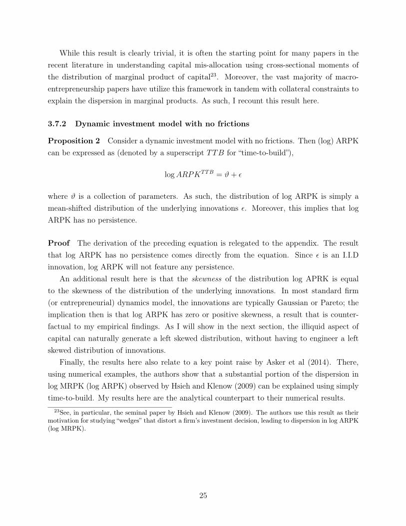
3.7.2 Dynamic investment model with no frictions

Proposition 2 Consider a dynamic investment model with no frictions. Then (log) ARPKcan be expressed as (denoted by a superscript TTB for “time-to-build”),

logARPKTTB = ϑ+ ε

where ϑ is a collection of parameters. As such, the distribution of log ARPK is simply amean-shifted distribution of the underlying innovations ε. Moreover, this implies that logARPK has no persistence.

Proof The derivation of the preceding equation is relegated to the appendix. The resultthat log ARPK has no persistence comes directly from the equation. Since ε is an I.I.Dinnovation, log ARPK will not feature any persistence.

An additional result here is that the skewness of the distribution log APRK is equalto the skewness of the distribution of the underlying innovations. In most standard firm(or entrepreneurial) dynamics model, the innovations are typically Gaussian or Pareto; theimplication then is that log ARPK has zero or positive skewness, a result that is counter-factual to my empirical findings. As I will show in the next section, the illiquid aspect ofcapital can naturally generate a left skewed distribution, without having to engineer a leftskewed distribution of innovations.

Finally, the results here also relate to a key point raise by Asker et al (2014). There,using numerical examples, the authors show that a substantial portion of the dispersion inlog MRPK (log ARPK) observed by Hsieh and Klenow (2009) can be explained using simplytime-to-build. My results here are the analytical counterpart to their numerical results.

23See, in particular, the seminal paper by Hsieh and Klenow (2009). The authors use this result as theirmotivation for studying “wedges” that distort a firm’s investment decision, leading to dispersion in log ARPK(log MRPK).

25

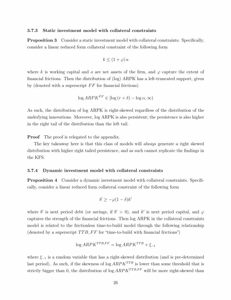
3.7.3 Static investment model with collateral constraints

Proposition 3 Consider a static investment model with collateral constraints. Specifically,consider a linear reduced form collateral constraint of the following form

k ≤ (1 + ϕ) a

where k is working capital and a are net assets of the firm, and ϕ capture the extent offinancial frictions. Then the distribution of (log) ARPK has a left-truncated support, givenby (denoted with a superscript FF for financial frictions)

logARPKFF ∈ [log (r + δ)− logα,∞)

As such, the distribution of log ARPK is right-skewed regardless of the distribution of theunderlying innovations. Moreover, log ARPK is also persistent; the persistence is also higherin the right tail of the distribution than the left tail.

Proof The proof is relegated to the appendix.The key takeaway here is that this class of models will always generate a right skewed

distribution with higher right tailed persistence, and as such cannot replicate the findings inthe KFS.

3.7.4 Dynamic investment model with collateral constraints

Proposition 4 Consider a dynamic investment model with collateral constraints. Specifi-cally, consider a linear reduced form collateral constraint of the following form

b′ ≥ −ϕ(1− δ)k′

where b′ is next period debt (or savings, if b′ > 0), and k′ is next period capital, and ϕ

captures the strength of the financial frictions. Then log ARPK in the collateral constraintsmodel is related to the frictionless time-to-build model through the following relationship(denoted by a superscript TTB, FF for “time-to-build with financial frictions”)

logARPKTTB,FF = logARPKTTB + ξ−1

where ξ−1 is a random variable that has a right-skewed distribution (and is pre-determinedlast period). As such, if the skewness of logARPKTTB is lower than some threshold that isstrictly bigger than 0, the distribution of logARPKTTB,FF will be more right-skewed than

26

the distribution of the underlying innovations. If the skewness of logARPKTTB if largerthan the threshold, than the distribution of logARPKTTB,FF is less right skewed than thedistribution of the underlying innovations, but it will always be right-skewed. Moreover, theright tail of the distribution will be more persistent than the left tail.

Proof The proof is relegated to the appendix.The key point here is that, like in the static model with collateral constraints, the dynamic

model will likewise feature a right skewed distribution of ARPK. As such, this class of modelswill not be able to replicate the results I presented in the earlier section.

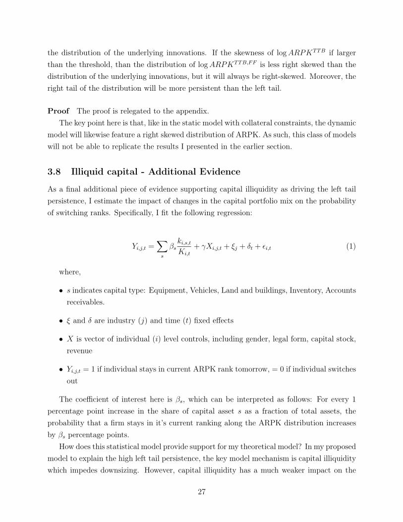
3.8 Illiquid capital - Additional Evidence

As a final additional piece of evidence supporting capital illiquidity as driving the left tailpersistence, I estimate the impact of changes in the capital portfolio mix on the probabilityof switching ranks. Specifically, I fit the following regression:

Yi,j,t =∑s

βski,s,tKi,t

+ γXi,j,t + ξj + δt + εi,t (1)

where,

• s indicates capital type: Equipment, Vehicles, Land and buildings, Inventory, Accountsreceivables.

• ξ and δ are industry (j) and time (t) fixed effects

• X is vector of individual (i) level controls, including gender, legal form, capital stock,revenue

• Yi,j,t = 1 if individual stays in current ARPK rank tomorrow, = 0 if individual switchesout

The coefficient of interest here is βs, which can be interpreted as follows: For every 1percentage point increase in the share of capital asset s as a fraction of total assets, theprobability that a firm stays in it’s current ranking along the ARPK distribution increasesby βs percentage points.

How does this statistical model provide support for my theoretical model? In my proposedmodel to explain the high left tail persistence, the key model mechanism is capital illiquiditywhich impedes downsizing. However, capital illiquidity has a much weaker impact on the

27

right tail, since it does not directly impede a firm from investing. As such, to the extentthat the capital types on the firm’s balance sheet have differential extent of liquidity, we cantest whether a firm that has more illiquid assets is also more likely to persist in a low ARPKstate; likewise, we can test whether a firm with more illiquid assets is more likely to persistis a high ARPK state.

Table 4 reports the regression results for firms that started out the period in rank 1 (i.e.firms in the bottom 20%) and rank 5 (i.e. firms in the top 20%). From column (1), we seethat firms that own a larger share of equipment, product inventories or land or buildings are(statistically and economically) significantly more likely to persist in a low ARPK state whenthey start the year with low ARPK. In contrast, firms that own a large share of vehicles andaccounts receivables are not statistically more likely to persist in their current state.

Notice that equipment and product inventory are highly firm specific, which makes resaleof these capital assets very difficult. Consequently, these assets can be considered highlyilliquid. Along the same vein, land and buildings are much less liquid due to the search costsassociated with selling them. As such, the results are suggestive that firms with greatershare of their assets invested in illiquid assets are also more likely to persist in a low ARPKstate.

In contrast, firms that have more of their assets invested in vehicles or accounts receivablesare not statistically more likely to persist in a low ARPK state. Unlike equipment or productinventory, vehicles are generally not firm specific. Moreover, there is a large market for resalevehicles. Accounts receivables are also relatively more liquid; unlike the previous assets whichare physical assets, these are debt owed to the firms.

In column (2), we see that firms that start out with high ARPK (i.e rank 5) are notaffected by their portfolio mix: none of the asset shares show any statistical significancewith respect to their effect on the probability that a high ARPK firm stays in the top 20%.This is reflective of the theory that capital illiquidity plays a very small role in driving theright tail persistence.

28

COEFFICIENT Pr(stay in rank 1) Pr(stay in rank 5)share of equipment 0.409** 0.400

(0.171) (0.247)share of inventory 0.701*** 0.287

(0.154) (0.291)share of vehicles 0.240 0.268

(0.177) (0.271)share of land / buildings 0.651*** -0.271

(0.188) (0.345)share of accounts receivables 0.0365 0.305

(0.171) (0.277)log(value added) -0.0500*** 0.0563**

(0.0162) (0.0223)log(real capital stock) 0.0368** -0.0577***

(0.0182) (0.0199)

Observations 1055 875R-squared 0.644 0.535Standard errors in parentheses*** p<0.01, ** p<0.05, * p<0.1

Table 4: Effect of portfolio share of each asset mix on probability that entrepreneur stays incurrent rank. Other controls (Year + Industry FE, gender, legal form) are included.

3.9 Parametric forms for productivity

Before moving forward to discussing the calibration strategy in the next section, I first closeout the model section by assigning functional forms to the productivity processes.

Business productivity Business productivity is assumed to follow an AR(1) process ofthe form log z′ = (1− ρz)µz+ρz log z+σzε

′z, with ε′z ∼ iid,N (0, 1). The process is discretized

with a 15 point Markov transition matrix using the Tauchen (1986) method.

Business productivity signal The signal is assumed to be drawn from a distorted in-variant distribution of the actual invariant distribution of business productivity. Note thatbusiness productivity has the invariant distribution N(µz,

√1

1−ρ2σz). In the case of thesignal, I assume worker households draw a signal from the "twisted" signal distributionN(µz,

√1

1−ρ2zσz), where the µz parameter distorts the household’s perception of the true

mean of the distribution of productivity. The primary effect of this is to vary the entry rate

29

into entrepreneurship, and thus steady-state population of entrepreneurs.

Labor productivity Labor productivity is assumed to follow an AR(1) process of theform log θ′ = (1− ρθ)µθ + ρθ log θ + σθε

′θ, with ε′θ ∼ iid,N (0, 1). The process is discretized

with a 15 point Markov transition matrix using the Tauchen (1986) method.

Labor productivity signal The signal is assumed to be drawn from a distorted in-variant distribution of the actual invariant distribution of labor productivity. Similar tothe case of business productivity signals, labor productivity has the invariant distributionN(µθ,

√1

1−ρ2θσθ); I assume then that entrepreneurial households draw a signal from the

“twisted" distribution N(µθ,√

11−ρ2θ

σθ), where µθ distorts the entrepreneur’s perception ofthe true mean of the distribution of labor productivity. The primary effect of this is to varythe exit rate.

4 Calibration

The model frequency is annual, which corresponds to the frequency in the KFS. As in theliterature, many standard parameters (such as the corporate sector’s capital share, deprecia-tion rate, labor income process) are taken from the preceding literature. The exact numbersused and their rationale are reported under “Group A" in table 5.

For “Group A" parameters, two parameters are set in an ad-hoc fashion: The value ofhome production c and the fraction of disinvestment that is considered small “η". Here, Iassume c = 0 and η = 1; therefore, I assume that home production has no value, and that anyvolume of transaction short of a complete exit is considered “small". I make this assumptionas there are no known references to which I can set these numbers to. Unfortunately, thereis also no clear strategy to discriminate the value of these parameters using the micro-data.However, as a further form of robustness checks, I experimented with different values of cand η, and found that the results are qualitatively very similar.

Three parameters are inferred directly from the data: The depreciation rate of the en-trepreneur’s capital stock δk, the capital intensity αk, and the returns to scale ν. Thedepreciation rate for the entrepreneur’s capital stock differs from the corporate sector, asthe composition of the aggregated “capital" stock is different for an entrepreneur as com-pared to that of a corporate firm. Consequently, I construct the depreciation rate for theentrepreneur’s capital as a weighted average of the individual depreciation rates of the com-ponents of the types of capital that make up an entrepreneur’s stock of capital. The capital

30

intensity and returns to scale are estimated using a hybrid cost shares approach and produc-tion function regression. The exact method from which these two parameters are constructedis relegated to the appendix. The estimated values used in the model is reported below under“Group B" in table 5.

Parameter Value Description Identifying momentGroup A parameters

γ Risk aversion 2 Standard. See for in-stance, Storesletten etal (2004)

µθ Unconditional mean oflabor productivity

0 Normalization

ρθ Persistence of labor pro-ductivity

0.94 Storesletten et al (2004)

σθ Conditional variance oflabor productivity

0.20 Storesletten et al (2004)

µz Mean of business pro-ductivity process pro-cess

0 Normalization

α Capital share of corpo-rate sector

0.33 Fixed to value inCagetti and De Nardi(2006)

A Corporate sector TFP 1 Normalizationδ Depreciation rate of

corporate sector capital0.10 Standard

η Parameter for “small"adjustment

1 See text

c Consumption value ofhome production

0 See text

Group B parametersδk 0.15 Depreciation rate of en-

trepreneur’s capitalFrom data (See ap-pendix)

αe 0.42 Capital intensity ofentrepreneurial produc-tion function

From data (See ap-pendix)

ν 0.79 Returns to scale ofentrepreneurial produc-tion function

From data (See ap-pendix)

Table 5: Fixed and estimated parameters

The rest of the ten parameters are inferred indirectly from the data by jointly calibratingthem to identifying moments from the data. A brief description of these parameters, as well

31

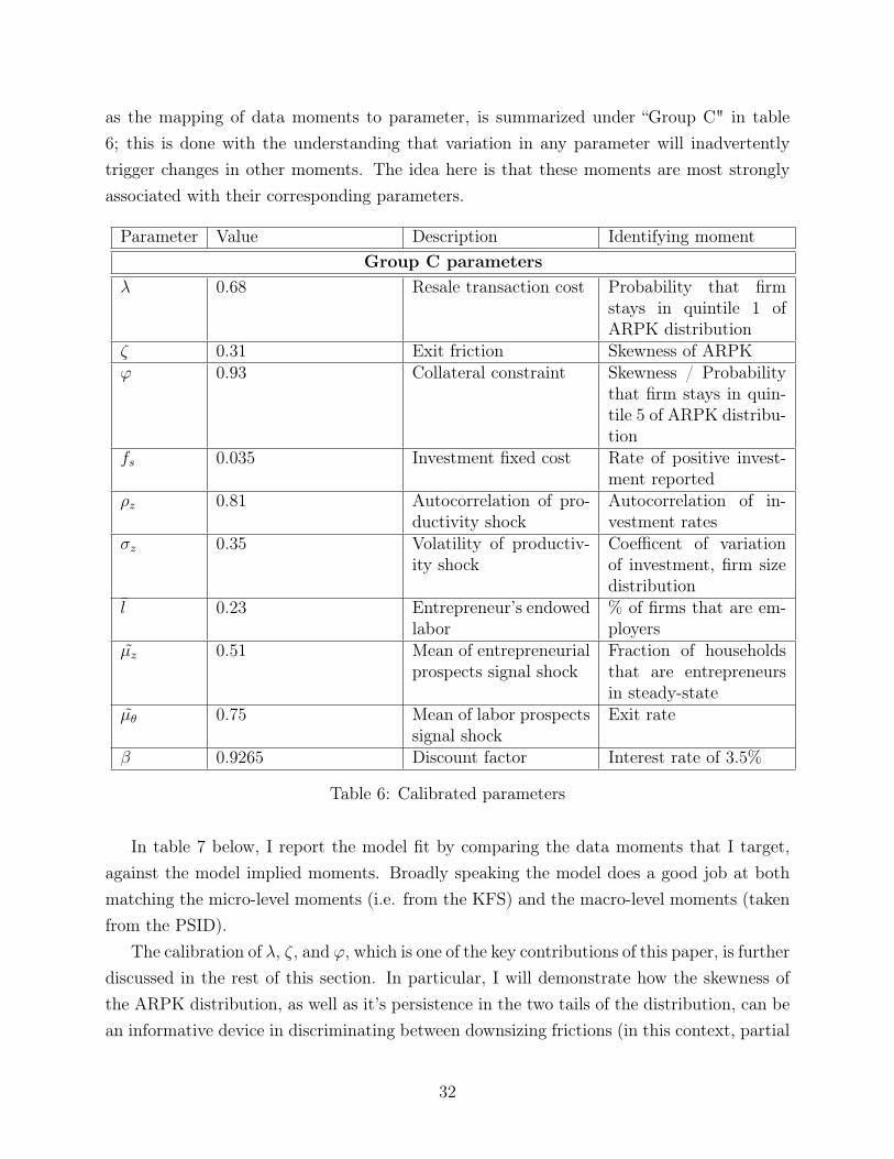
as the mapping of data moments to parameter, is summarized under “Group C" in table6; this is done with the understanding that variation in any parameter will inadvertentlytrigger changes in other moments. The idea here is that these moments are most stronglyassociated with their corresponding parameters.

Parameter Value Description Identifying momentGroup C parameters

λ 0.68 Resale transaction cost Probability that firmstays in quintile 1 ofARPK distribution

ζ 0.31 Exit friction Skewness of ARPKϕ 0.93 Collateral constraint Skewness / Probability

that firm stays in quin-tile 5 of ARPK distribu-tion

fs 0.035 Investment fixed cost Rate of positive invest-ment reported

ρz 0.81 Autocorrelation of pro-ductivity shock

Autocorrelation of in-vestment rates

σz 0.35 Volatility of productiv-ity shock

Coefficent of variationof investment, firm sizedistribution

l 0.23 Entrepreneur’s endowedlabor

% of firms that are em-ployers

µz 0.51 Mean of entrepreneurialprospects signal shock

Fraction of householdsthat are entrepreneursin steady-state

µθ 0.75 Mean of labor prospectssignal shock

Exit rate

β 0.9265 Discount factor Interest rate of 3.5%

Table 6: Calibrated parameters

In table 7 below, I report the model fit by comparing the data moments that I target,against the model implied moments. Broadly speaking the model does a good job at bothmatching the micro-level moments (i.e. from the KFS) and the macro-level moments (takenfrom the PSID).

The calibration of λ, ζ, and ϕ, which is one of the key contributions of this paper, is furtherdiscussed in the rest of this section. In particular, I will demonstrate how the skewness ofthe ARPK distribution, as well as it’s persistence in the two tails of the distribution, can bean informative device in discriminating between downsizing frictions (in this context, partial

32

irreversibility) and investment frictions (such as collateral constraints). The calibration ofthe other parameters are relegated to the appendix.

Moments Data ModelPr(1,1) 0.58 0.57Pr(5,5) 0.47 0.44Skew log(Y/K) -0.39 -0.29% +ve investment 54% 50%CV of I/K 4.0 4.0% Employer firms 53% 58%KFS exit rate 10% 30%% of households that are en-trepreneurs

(8%,20%) 8.9%

% Exit rate (20%,40%) 32%% Startup rate (3%,10%) 3.2Interest rate 3.5% 3.5

Table 7: Model fit: Data and corresponding model moments

4.1 Downsizing frictions and collateral constraints: Skewness and

asymmetric persistence

How important are the downsizing frictions in helping the model to match the skewnessand asymmetric persistence noted in the data? Table 8 below reports the model impliedmoments for the skewness and the tail persistence when the resale frictions are removed (i.e.λ = ζ = 0).

Moment Data Benchmark calibration Counter-factual: No resale frictionsTargeted

skew(log Y

K

)-0.39 -0.29 0.18

Pr(1→ 1) 0.58 0.57 0.37Pr(5→ 5) 0.47 0.44 0.47

Not targetedρ1 0.71 0.84 0.31ρ5 0.45 0.50 0.63

Table 8: Effect of illiquidity on skewness and symmetric persistence - Comparison withcounter-factual “frictionless" model. ρ1 and ρ5 refer to the autocorrelation of ARPK inquintile 1 and 5 respectively. These two moments were not targeted.

Notice that once the two resale frictions are removed, the overall skewness rises to 0.18;that is, the distribution is now right-skewed, as predicted in the earlier section. Similarly,

33

the left-tail persistence falls to 0.37, whereas the right-tail persistence rises to 0.47. In otherwords, the model now exhibits greater persistence in the right tail than the left tail. Asa form of external validation, I also report the effect on the autocorrelation of ARPK inthe bottom and top quintiles; these two moments are not explicitly targeted. Similar to thefinding with the persistence of relative rankings, the benchmark calibration generates greaterautocorrelation in the left than right tail. In contrast, a model without resale frictions flipsthe asymmetry.

Why is modeling resale frictions so crucial in generating the left skewness and higher lefttail persistence?

First, recall that in a fully frictionless economy, all firms always target the same (expected)ARPK. Ex-post, the distribution of ARPK then simply reflects the distribution of all theindividuals’ expectational errors; in the case of i.i.d log-normal innovations, for example, theARPK distribution is also log-normal and has no persistence.

Next, when the same model is augmented with collateral constraints, firm that are fi-nancially unconstrained behave just as the firms in the frictionless economy. As such, theconditional distribution (of unconstrained firms) simply reflects the expectational errors.Again, when innovations are i.i.d log-normal as assumed in the benchmark calibration, thisconditional distribution will have no skewness or persistence. Financially constrained firms,on the other hand, must necessarily operate firm sizes that are “too small" relative to theiroptimal sizes - that is, their ARPK must be higher than the optimal ARPK (in expecta-tion). Consequently, the ex-post conditional distribution of constrained firms will featurea right skew, and the combined distribution of constrained and unconstrained firms is alsoright-skewed. Moreover, the tighter the collateral constraint, the more right-skewed thedistribution will be, as one can see in the bottom panel of figure 3a.

In contrast, downsizing frictions tend to extend the left tail of the distribution. Whenhit by a bad shock, the options value of capital induced by the asymmetry in purchase andresale price of capital lead downsizing entrepreneurs to target a lower ARPK (in expectation)than the unconstrained ARPK. As a result, the left tail of the ARPK distribution becomesextended, making the distribution more left-skewed. Moreover, resale frictions also lead poorperforming entrepreneurs to stay in business for longer periods of time. The combined effectgenerates greater left skewness when these frictions are added to the model. This result isreflected in the first top panel of figure 3a.

34

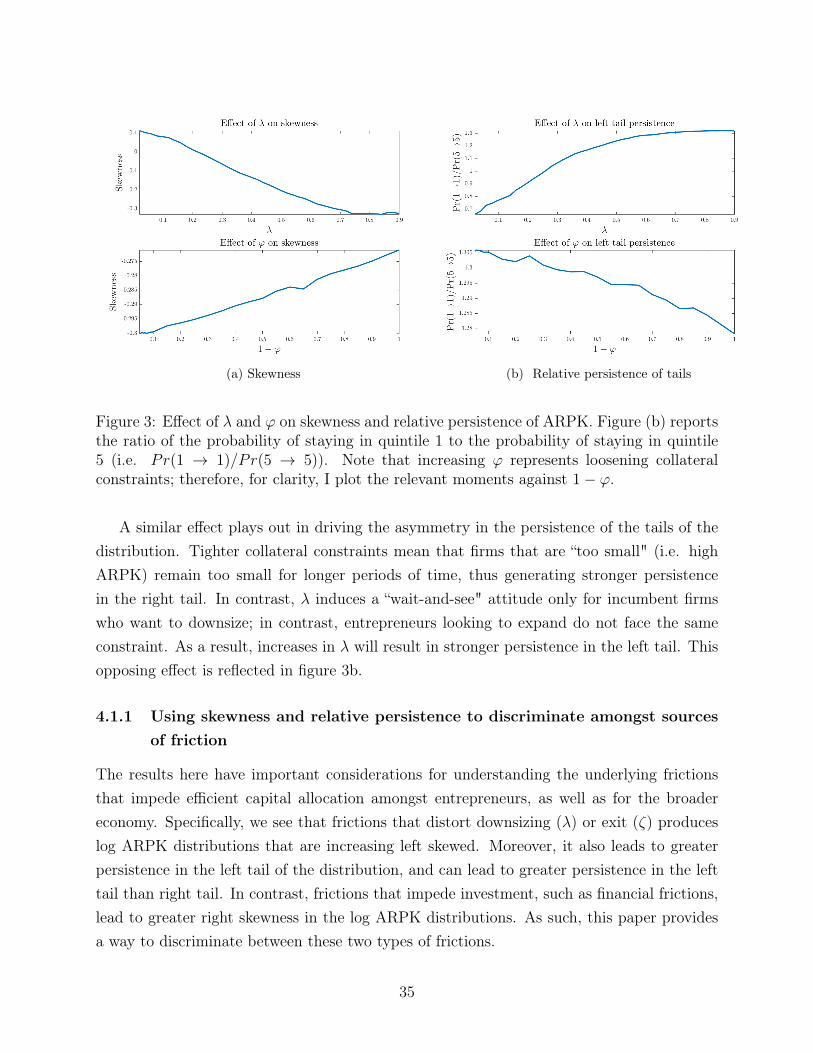
(a) Skewness (b) Relative persistence of tails

Figure 3: Effect of λ and ϕ on skewness and relative persistence of ARPK. Figure (b) reportsthe ratio of the probability of staying in quintile 1 to the probability of staying in quintile5 (i.e. Pr(1 → 1)/Pr(5 → 5)). Note that increasing ϕ represents loosening collateralconstraints; therefore, for clarity, I plot the relevant moments against 1− ϕ.

A similar effect plays out in driving the asymmetry in the persistence of the tails of thedistribution. Tighter collateral constraints mean that firms that are “too small" (i.e. highARPK) remain too small for longer periods of time, thus generating stronger persistencein the right tail. In contrast, λ induces a “wait-and-see" attitude only for incumbent firmswho want to downsize; in contrast, entrepreneurs looking to expand do not face the sameconstraint. As a result, increases in λ will result in stronger persistence in the left tail. Thisopposing effect is reflected in figure 3b.

4.1.1 Using skewness and relative persistence to discriminate amongst sourcesof friction

The results here have important considerations for understanding the underlying frictionsthat impede efficient capital allocation amongst entrepreneurs, as well as for the broadereconomy. Specifically, we see that frictions that distort downsizing (λ) or exit (ζ) produceslog ARPK distributions that are increasing left skewed. Moreover, it also leads to greaterpersistence in the left tail of the distribution, and can lead to greater persistence in the lefttail than right tail. In contrast, frictions that impede investment, such as financial frictions,lead to greater right skewness in the log ARPK distributions. As such, this paper providesa way to discriminate between these two types of frictions.

35

In contrast, prior papers that focus on misallocation of capital, such as Hsieh and Klenow(2009), Asker et al (2014), and Midrigan and Xu (2014), have focused primarily on studyingthe dispersion of log MRPK (and equivalently, log ARPK). Asker et al (2014), for instance,focuses on capital adjustment costs (equivalent to the fs and λ parameters in this model)while ignoring financing constraints, while Midrigan and Xu (2014) focuses on financing con-straints (equivalent to ϕ in this model) but largely abstracting away from adjustment costs.In both cases, frictions can lead to observationally equivalent outcomes in the dispersion oflog MRPK (or ARPK). This paper therefore merges these two frameworks by incorporatingboth adjustment and financial frictions, and providing a simple framework to discriminatebetween the two (i.e. using the skewness and relative persistence).

4.1.2 Are entrepreneurs financially constrained?

In the benchmark calibration, ϕ = 0.93. ϕ in this model refers to the limited commitmentproblem in the Kiyotaki-Moore framework; in this context, this means that entrepreneursare able to collateralize up to 93% of the face value of their capital assets.

What does this mean? At face value, this suggests that early stage entrepreneurs are infact less encumbered by financial frictions than one suspects. In prior research such as thatin Evans and Jovanovic (1989) or Cagetti and De Nardi (2006), financial friction play a largerole in determining the dispersion of wealth and firm sizes24. The inability to fully borrow andfund their investment leads to large distortions in the economy, primarily by deterring highproductivity potential entrants from entering, and forcing poorer entrepreneurs to run sub-optimally small firms. In contrast, my results appear to be more in line with that reportedin Hurst and Lusardi (2004), Nanda (2011), and Robb and Robinson (2014), which find noevidence that regular entrepreneurs face severe financing constraints. In particular, Robband Robinson (2014), using the same data set as this paper, find that most entrepreneursare able to finance their investment by simply going to the bank.

Does this mean that entrepreneurs don’t face borrowing constraints? On the contrary,the calibration indicates that entrepreneurs face tight collateral constraints similar to that inthe preceding literature. Note that while ϕ determines the financial frictions that arise fromthe limited commitment problem, the true collateral constraint is given by ϕ ≡ (1− λ)× ϕ,i.e. the entrepreneur can only collateralize the net depreciated resale value of entrepreneurialcapital. When this effect is taken into account, the “net collateral constraint" parameter ϕ isabout 0.30, i.e. 30% of the real value of entrepreneurial capital is collateralizable. Given that

24Evans and Jovanovic (1989) report an equivalent point estimate of 0.44, Cagetti and De Nardi (2006)uses a benchmark calibration that amounts to 0.25 in this model. Other similar papers such as Kitao (2008)and Beura and Shin (2013) generally assume an equivalent collateral constraint of 0.33.

36

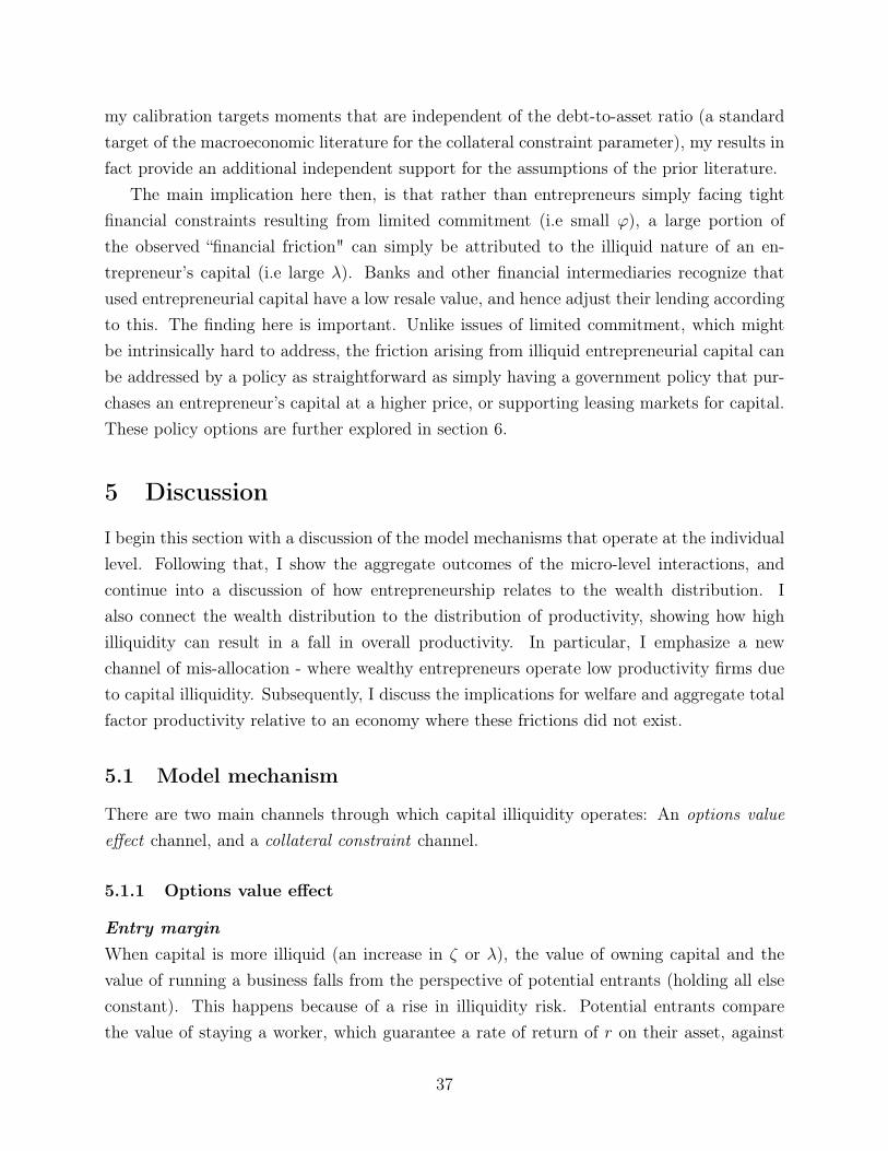
my calibration targets moments that are independent of the debt-to-asset ratio (a standardtarget of the macroeconomic literature for the collateral constraint parameter), my results infact provide an additional independent support for the assumptions of the prior literature.

The main implication here then, is that rather than entrepreneurs simply facing tightfinancial constraints resulting from limited commitment (i.e small ϕ), a large portion ofthe observed “financial friction" can simply be attributed to the illiquid nature of an en-trepreneur’s capital (i.e large λ). Banks and other financial intermediaries recognize thatused entrepreneurial capital have a low resale value, and hence adjust their lending accordingto this. The finding here is important. Unlike issues of limited commitment, which mightbe intrinsically hard to address, the friction arising from illiquid entrepreneurial capital canbe addressed by a policy as straightforward as simply having a government policy that pur-chases an entrepreneur’s capital at a higher price, or supporting leasing markets for capital.These policy options are further explored in section 6.

5 Discussion

I begin this section with a discussion of the model mechanisms that operate at the individuallevel. Following that, I show the aggregate outcomes of the micro-level interactions, andcontinue into a discussion of how entrepreneurship relates to the wealth distribution. Ialso connect the wealth distribution to the distribution of productivity, showing how highilliquidity can result in a fall in overall productivity. In particular, I emphasize a newchannel of mis-allocation - where wealthy entrepreneurs operate low productivity firms dueto capital illiquidity. Subsequently, I discuss the implications for welfare and aggregate totalfactor productivity relative to an economy where these frictions did not exist.

5.1 Model mechanism

There are two main channels through which capital illiquidity operates: An options valueeffect channel, and a collateral constraint channel.

5.1.1 Options value effect

Entry marginWhen capital is more illiquid (an increase in ζ or λ), the value of owning capital and thevalue of running a business falls from the perspective of potential entrants (holding all elseconstant). This happens because of a rise in illiquidity risk. Potential entrants comparethe value of staying a worker, which guarantee a rate of return of r on their asset, against

37

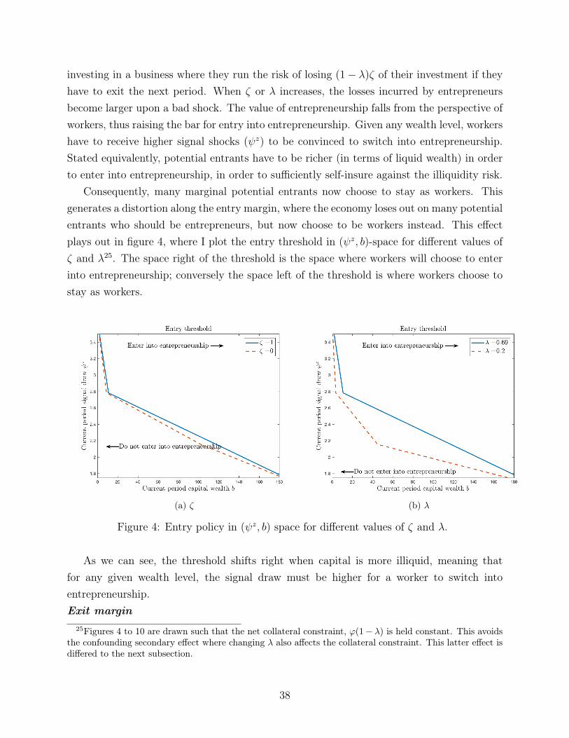
investing in a business where they run the risk of losing (1− λ)ζ of their investment if theyhave to exit the next period. When ζ or λ increases, the losses incurred by entrepreneursbecome larger upon a bad shock. The value of entrepreneurship falls from the perspective ofworkers, thus raising the bar for entry into entrepreneurship. Given any wealth level, workershave to receive higher signal shocks (ψz) to be convinced to switch into entrepreneurship.Stated equivalently, potential entrants have to be richer (in terms of liquid wealth) in orderto enter into entrepreneurship, in order to sufficiently self-insure against the illiquidity risk.

Consequently, many marginal potential entrants now choose to stay as workers. Thisgenerates a distortion along the entry margin, where the economy loses out on many potentialentrants who should be entrepreneurs, but now choose to be workers instead. This effectplays out in figure 4, where I plot the entry threshold in (ψz, b)-space for different values ofζ and λ25. The space right of the threshold is the space where workers will choose to enterinto entrepreneurship; conversely the space left of the threshold is where workers choose tostay as workers.

(a) ζ (b) λ

Figure 4: Entry policy in (ψz, b) space for different values of ζ and λ.

As we can see, the threshold shifts right when capital is more illiquid, meaning thatfor any given wealth level, the signal draw must be higher for a worker to switch intoentrepreneurship.Exit margin

25Figures 4 to 10 are drawn such that the net collateral constraint, ϕ(1− λ) is held constant. This avoidsthe confounding secondary effect where changing λ also affects the collateral constraint. This latter effect isdiffered to the next subsection.

38

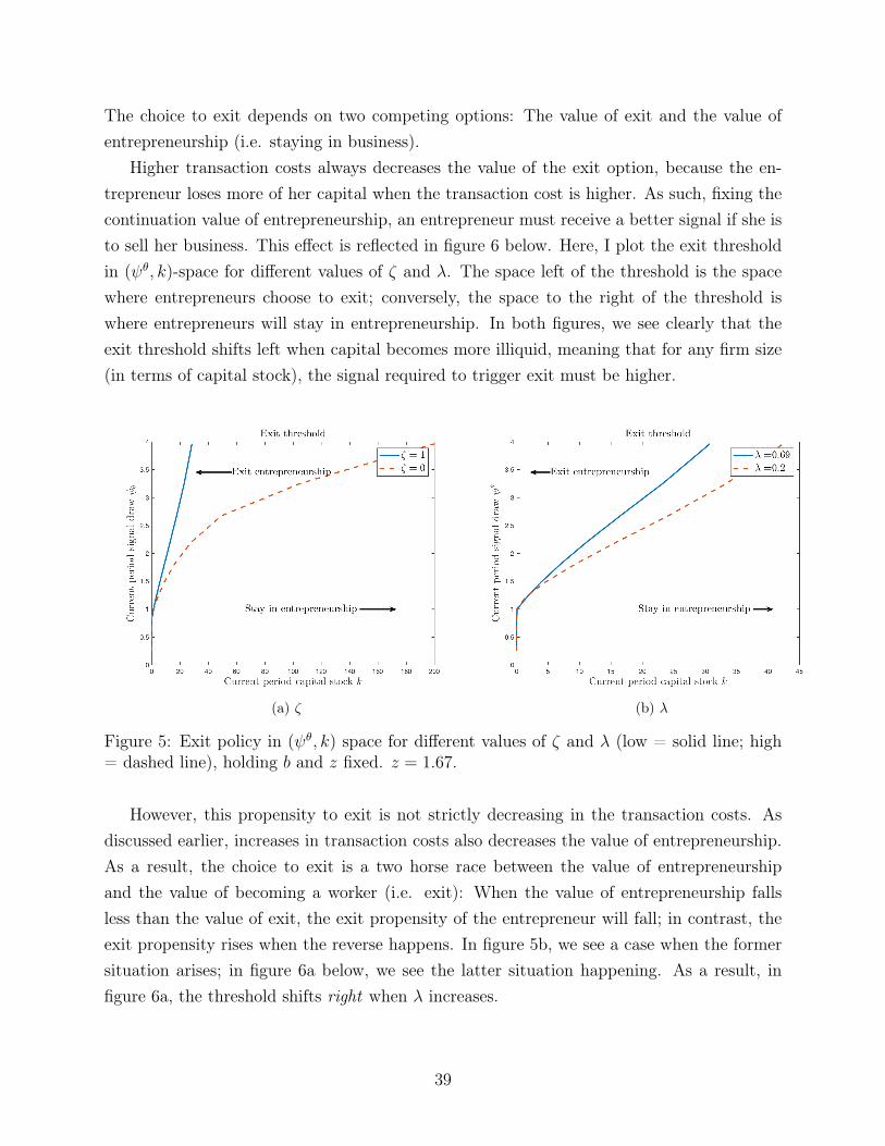
The choice to exit depends on two competing options: The value of exit and the value ofentrepreneurship (i.e. staying in business).

Higher transaction costs always decreases the value of the exit option, because the en-trepreneur loses more of her capital when the transaction cost is higher. As such, fixing thecontinuation value of entrepreneurship, an entrepreneur must receive a better signal if she isto sell her business. This effect is reflected in figure 6 below. Here, I plot the exit thresholdin (ψθ, k)-space for different values of ζ and λ. The space left of the threshold is the spacewhere entrepreneurs choose to exit; conversely, the space to the right of the threshold iswhere entrepreneurs will stay in entrepreneurship. In both figures, we see clearly that theexit threshold shifts left when capital becomes more illiquid, meaning that for any firm size(in terms of capital stock), the signal required to trigger exit must be higher.

(a) ζ (b) λ

Figure 5: Exit policy in (ψθ, k) space for different values of ζ and λ (low = solid line; high= dashed line), holding b and z fixed. z = 1.67.

However, this propensity to exit is not strictly decreasing in the transaction costs. Asdiscussed earlier, increases in transaction costs also decreases the value of entrepreneurship.As a result, the choice to exit is a two horse race between the value of entrepreneurshipand the value of becoming a worker (i.e. exit): When the value of entrepreneurship fallsless than the value of exit, the exit propensity of the entrepreneur will fall; in contrast, theexit propensity rises when the reverse happens. In figure 5b, we see a case when the formersituation arises; in figure 6a below, we see the latter situation happening. As a result, infigure 6a, the threshold shifts right when λ increases.

39

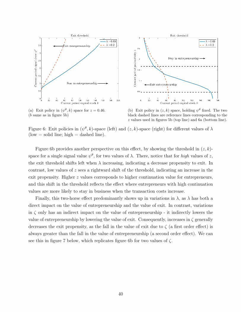
(a) Exit policy in (ψθ, k) space for z = 0.46.(b same as in figure 5b)

(b) Exit policy in (z, k) space, holding ψθ fixed. The twoblack dashed lines are reference lines corresponding to thez values used in figures 5b (top line) and 6a (bottom line).

Figure 6: Exit policies in (ψθ, k)-space (left) and (z, k)-space (right) for different values of λ(low = solid line; high = dashed line).

Figure 6b provides another perspective on this effect, by showing the threshold in (z, k)-space for a single signal value ψθ, for two values of λ. There, notice that for high values of z,the exit threshold shifts left when λ increasing, indicating a decrease propensity to exit. Incontrast, low values of z sees a rightward shift of the threshold, indicating an increase in theexit propensity. Higher z values corresponds to higher continuation value for entrepreneurs,and this shift in the threshold reflects the effect where entrepreneurs with high continuationvalues are more likely to stay in business when the transaction costs increase.

Finally, this two-horse effect predominantly shows up in variations in λ, as λ has both adirect impact on the value of entrepreneurship and the value of exit. In contrast, variationsin ζ only has an indirect impact on the value of entrepreneurship - it indirectly lowers thevalue of entrepreneurship by lowering the value of exit. Consequently, increases in ζ generallydecreases the exit propensity, as the fall in the value of exit due to ζ (a first order effect) isalways greater than the fall in the value of entrepreneurship (a second order effect). We cansee this in figure 7 below, which replicates figure 6b for two values of ζ.

40

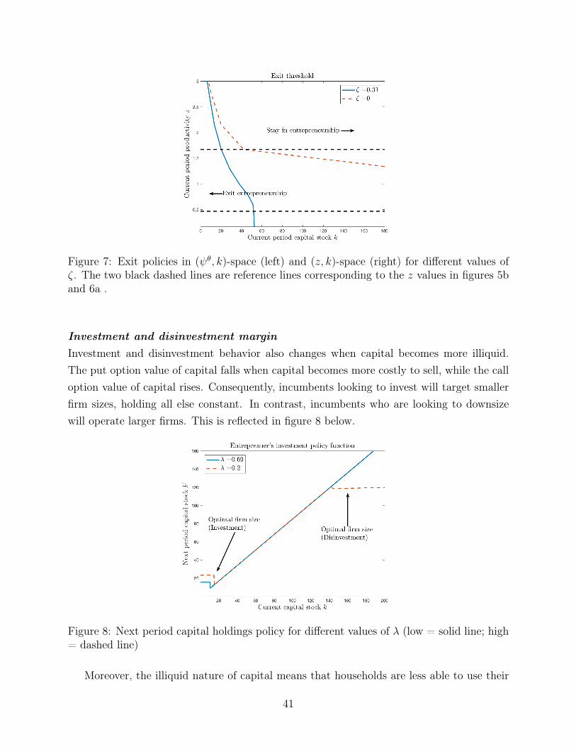
Figure 7: Exit policies in (ψθ, k)-space (left) and (z, k)-space (right) for different values ofζ. The two black dashed lines are reference lines corresponding to the z values in figures 5band 6a .

Investment and disinvestment marginInvestment and disinvestment behavior also changes when capital becomes more illiquid.The put option value of capital falls when capital becomes more costly to sell, while the calloption value of capital rises. Consequently, incumbents looking to invest will target smallerfirm sizes, holding all else constant. In contrast, incumbents who are looking to downsizewill operate larger firms. This is reflected in figure 8 below.

Figure 8: Next period capital holdings policy for different values of λ (low = solid line; high= dashed line)

Moreover, the illiquid nature of capital means that households are less able to use their

41

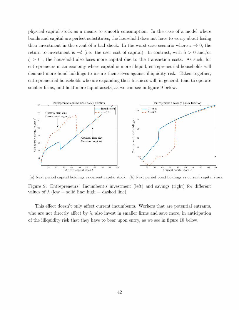
physical capital stock as a means to smooth consumption. In the case of a model wherebonds and capital are perfect substitutes, the household does not have to worry about losingtheir investment in the event of a bad shock. In the worst case scenario where z → 0, thereturn to investment is −δ (i.e. the user cost of capital). In contrast, with λ > 0 and/orζ > 0 , the household also loses more capital due to the transaction costs. As such, forentrepreneurs in an economy where capital is more illiquid, entrepreneurial households willdemand more bond holdings to insure themselves against illiquidity risk. Taken together,entrepreneurial households who are expanding their business will, in general, tend to operatesmaller firms, and hold more liquid assets, as we can see in figure 9 below.

(a) Next period capital holdings vs current capital stock (b) Next period bond holdings vs current capital stock

Figure 9: Entrepreneurs: Incumbent’s investment (left) and savings (right) for differentvalues of λ (low = solid line; high = dashed line)

This effect doesn’t only affect current incumbents. Workers that are potential entrants,who are not directly affect by λ, also invest in smaller firms and save more, in anticipationof the illiquidity risk that they have to bear upon entry, as we see in figure 10 below.

42

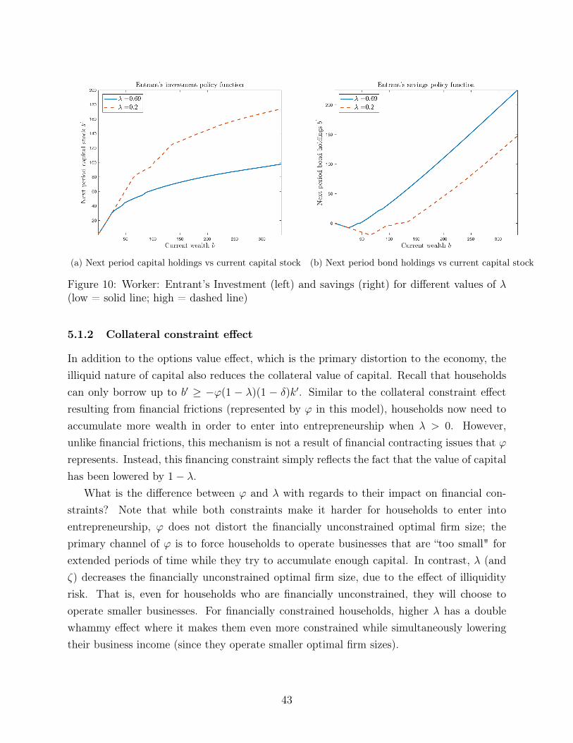
(a) Next period capital holdings vs current capital stock (b) Next period bond holdings vs current capital stock

Figure 10: Worker: Entrant’s Investment (left) and savings (right) for different values of λ(low = solid line; high = dashed line)

5.1.2 Collateral constraint effect

In addition to the options value effect, which is the primary distortion to the economy, theilliquid nature of capital also reduces the collateral value of capital. Recall that householdscan only borrow up to b′ ≥ −ϕ(1 − λ)(1 − δ)k′. Similar to the collateral constraint effectresulting from financial frictions (represented by ϕ in this model), households now need toaccumulate more wealth in order to enter into entrepreneurship when λ > 0. However,unlike financial frictions, this mechanism is not a result of financial contracting issues that ϕrepresents. Instead, this financing constraint simply reflects the fact that the value of capitalhas been lowered by 1− λ.

What is the difference between ϕ and λ with regards to their impact on financial con-straints? Note that while both constraints make it harder for households to enter intoentrepreneurship, ϕ does not distort the financially unconstrained optimal firm size; theprimary channel of ϕ is to force households to operate businesses that are “too small" forextended periods of time while they try to accumulate enough capital. In contrast, λ (andζ) decreases the financially unconstrained optimal firm size, due to the effect of illiquidityrisk. That is, even for households who are financially unconstrained, they will choose tooperate smaller businesses. For financially constrained households, higher λ has a doublewhammy effect where it makes them even more constrained while simultaneously loweringtheir business income (since they operate smaller optimal firm sizes).

43

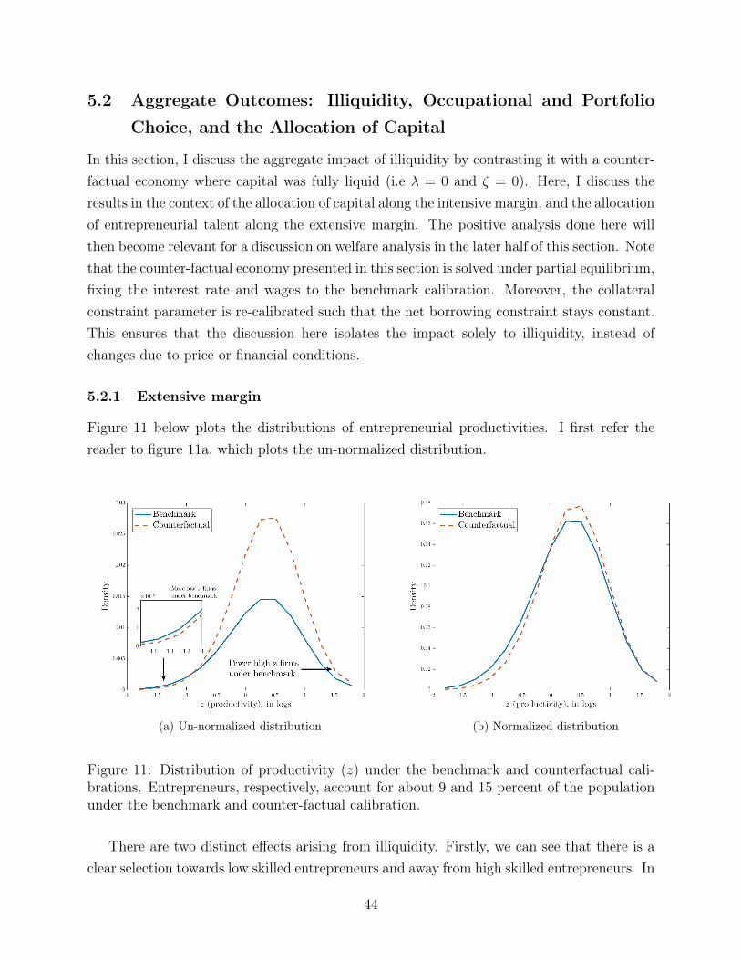
5.2 Aggregate Outcomes: Illiquidity, Occupational and Portfolio

Choice, and the Allocation of Capital

In this section, I discuss the aggregate impact of illiquidity by contrasting it with a counter-factual economy where capital was fully liquid (i.e λ = 0 and ζ = 0). Here, I discuss theresults in the context of the allocation of capital along the intensive margin, and the allocationof entrepreneurial talent along the extensive margin. The positive analysis done here willthen become relevant for a discussion on welfare analysis in the later half of this section. Notethat the counter-factual economy presented in this section is solved under partial equilibrium,fixing the interest rate and wages to the benchmark calibration. Moreover, the collateralconstraint parameter is re-calibrated such that the net borrowing constraint stays constant.This ensures that the discussion here isolates the impact solely to illiquidity, instead ofchanges due to price or financial conditions.

5.2.1 Extensive margin

Figure 11 below plots the distributions of entrepreneurial productivities. I first refer thereader to figure 11a, which plots the un-normalized distribution.

(a) Un-normalized distribution (b) Normalized distribution

Figure 11: Distribution of productivity (z) under the benchmark and counterfactual cali-brations. Entrepreneurs, respectively, account for about 9 and 15 percent of the populationunder the benchmark and counter-factual calibration.

There are two distinct effects arising from illiquidity. Firstly, we can see that there is aclear selection towards low skilled entrepreneurs and away from high skilled entrepreneurs. In

44

the left tail of the distribution, we see that there are more low skilled entrepreneurs under thebenchmark calibration; in the right tail, we see that there are less high skilled entrepreneursunder the benchmark calibration. This happens because of the options value effect discussedearlier. For low skilled entrepreneurs, the wait-and-see effect generated by the exit costs leadthem to persist longer, therefore giving rise to more low skilled entrepreneurs. For high skilledentrepreneurs, the distortion along the entry margin means that even conditional on the samesignal, potential entrants need to be wealthier in order to enter into entrepreneurship. Asa result, there are less high skilled entrepreneurs under the benchmark calibration. Noticethat this result is not simply a consequence of the lack of normalization. In figure 11b, wesee that the effect persists; in fact, it becomes even starker on the left tail.

Secondly, illiquidity also leads to a fall in the size of the population of entrepreneurs. Wecan see this from the un-normalized distribution, where the area under the density function ofthe counter-factual economy is visually bigger than that of the benchmark calibration. Thefact that this population falls is not an obvious result, but rather the interaction betweenthe exit and entry rates along the transition path towards the steady state.

To understand this point, first recall from the earlier discussion that decreases in theresale value of capital will always lead to a fall in the propensity of entry, but have anambiguous impact on the propensity to exit. However, in steady-state, as the exit rate mustalways equate the entry rate, the net result of falling resale values means that the overallrate of reallocation at the extensive margin (i.e. the equilibrium rate at which householdsswitch occupations) must fall. Indeed, this is reflected in figure 12, which plots the numberof households who are entering entrepreneurship in steady-state, as a function of ζ (bottomfigure) and λ (top figure).

45

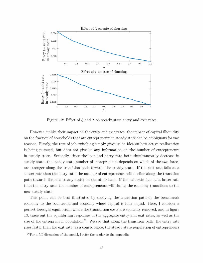
Figure 12: Effect of ζ and λ on steady state entry and exit rates

However, unlike their impact on the entry and exit rates, the impact of capital illiquidityon the fraction of households that are entrepreneurs in steady state can be ambiguous for tworeasons. Firstly, the rate of job switching simply gives us an idea on how active reallocationis being pursued, but does not give us any information on the number of entrepreneursin steady state. Secondly, since the exit and entry rate both simultaneously decrease insteady-state, the steady state number of entrepreneurs depends on which of the two forcesare stronger along the transition path towards the steady state. If the exit rate falls at aslower rate than the entry rate, the number of entrepreneurs will decline along the transitionpath towards the new steady state; on the other hand, if the exit rate falls at a faster ratethan the entry rate, the number of entrepreneurs will rise as the economy transitions to thenew steady state.

This point can be best illustrated by studying the transition path of the benchmarkeconomy to the counter-factual economy where capital is fully liquid. Here, I consider aperfect foresight equilibrium where the transaction costs are suddenly removed, and in figure13, trace out the equilibrium responses of the aggregate entry and exit rates, as well as thesize of the entrepreneur population26. We see that along the transition path, the entry raterises faster than the exit rate; as a consequence, the steady state population of entrepreneurs

26For a full discussion of the model, I refer the reader to the appendix

46

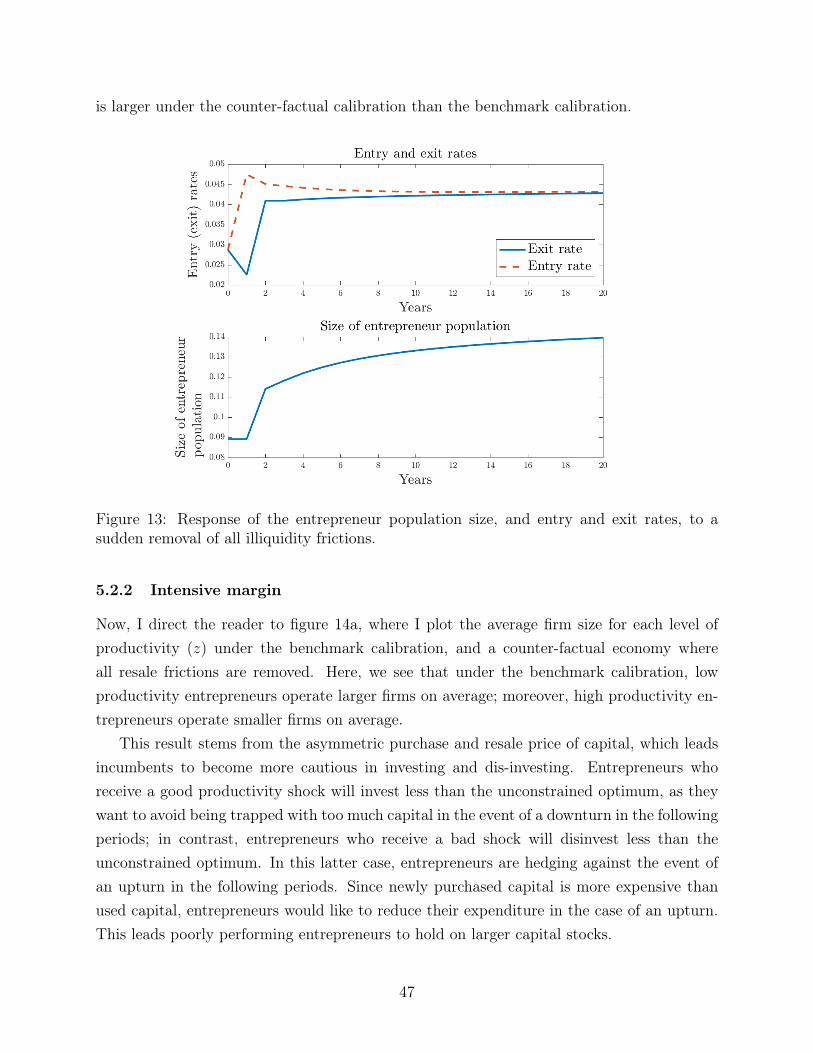
is larger under the counter-factual calibration than the benchmark calibration.

Figure 13: Response of the entrepreneur population size, and entry and exit rates, to asudden removal of all illiquidity frictions.

5.2.2 Intensive margin

Now, I direct the reader to figure 14a, where I plot the average firm size for each level ofproductivity (z) under the benchmark calibration, and a counter-factual economy whereall resale frictions are removed. Here, we see that under the benchmark calibration, lowproductivity entrepreneurs operate larger firms on average; moreover, high productivity en-trepreneurs operate smaller firms on average.

This result stems from the asymmetric purchase and resale price of capital, which leadsincumbents to become more cautious in investing and dis-investing. Entrepreneurs whoreceive a good productivity shock will invest less than the unconstrained optimum, as theywant to avoid being trapped with too much capital in the event of a downturn in the followingperiods; in contrast, entrepreneurs who receive a bad shock will disinvest less than theunconstrained optimum. In this latter case, entrepreneurs are hedging against the event ofan upturn in the following periods. Since newly purchased capital is more expensive thanused capital, entrepreneurs would like to reduce their expenditure in the case of an upturn.This leads poorly performing entrepreneurs to hold on larger capital stocks.

47

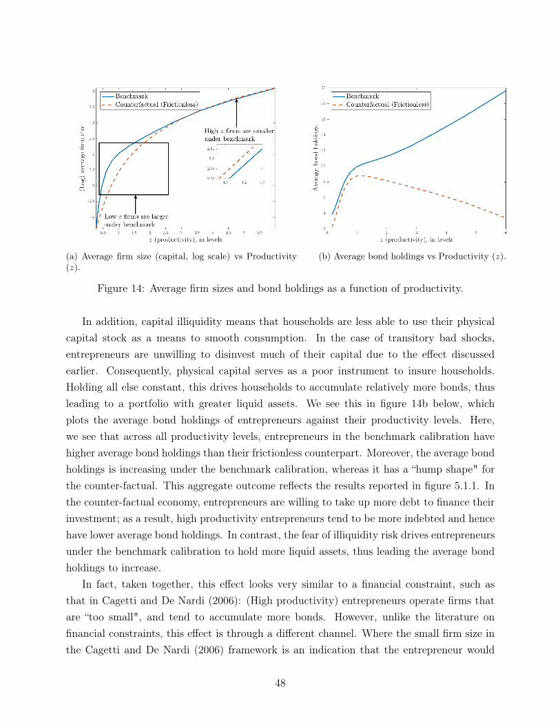
(a) Average firm size (capital, log scale) vs Productivity(z).

(b) Average bond holdings vs Productivity (z).

Figure 14: Average firm sizes and bond holdings as a function of productivity.

In addition, capital illiquidity means that households are less able to use their physicalcapital stock as a means to smooth consumption. In the case of transitory bad shocks,entrepreneurs are unwilling to disinvest much of their capital due to the effect discussedearlier. Consequently, physical capital serves as a poor instrument to insure households.Holding all else constant, this drives households to accumulate relatively more bonds, thusleading to a portfolio with greater liquid assets. We see this in figure 14b below, whichplots the average bond holdings of entrepreneurs against their productivity levels. Here,we see that across all productivity levels, entrepreneurs in the benchmark calibration havehigher average bond holdings than their frictionless counterpart. Moreover, the average bondholdings is increasing under the benchmark calibration, whereas it has a “hump shape" forthe counter-factual. This aggregate outcome reflects the results reported in figure 5.1.1. Inthe counter-factual economy, entrepreneurs are willing to take up more debt to finance theirinvestment; as a result, high productivity entrepreneurs tend to be more indebted and hencehave lower average bond holdings. In contrast, the fear of illiquidity risk drives entrepreneursunder the benchmark calibration to hold more liquid assets, thus leading the average bondholdings to increase.

In fact, taken together, this effect looks very similar to a financial constraint, such asthat in Cagetti and De Nardi (2006): (High productivity) entrepreneurs operate firms thatare “too small", and tend to accumulate more bonds. However, unlike the literature onfinancial constraints, this effect is through a different channel. Where the small firm size inthe Cagetti and De Nardi (2006) framework is an indication that the entrepreneur would

48

like to expand if she could, the smaller firm sizes here is a result of households simply havingno desire to expand to the unconstrained optimum. Likewise, where wealth accumulation inthe face of financial frictions results from households trying to save out of their constraints,higher (liquid) wealth accumulation here is simply a result of households trying to self-insureagainst illiquidity risk.

5.3 The Wealth Distribution

Table 9 below reports the wealth distribution in the US (row 5), and contrasts the modelpredicted wealth distribution under the benchmark calibration (row 1), and a counter-factualeconomy where there are no resale frictions. For the model with no resale frictions, I reset thecollateral constraint parameter to ϕ, such that ϕ = (1− λ)ϕ, thus keeping the net collateralconstraint constant. The no resale friction model is solved under partial equilibrium (row2), where I keep the interest rate r at the benchmark calibration, as well as under generalequilibrium (row 3). It also reports the Gini coefficient as a single summary statistic for theextent of wealth inequality predicted by the model. I also report the wealth distribution foran equivalent model where entrepreneurship is not modeled (i.e. the plain Aiyagari model).

Concentrationof wealth in:

Quintile range Top 10% Gini

Model/Data 1st 2nd 3rd 4th 5th 90-95 95-99 99-100

(1) Benchmark 1.5 4.2 7.9 15 72 11 23 23 0.68(2) Frictionless(PE)

1.1 3 5.7 11 83 14 28 25 0.75

(3) Frictionless(GE)

1.1 3 5.5 11 80 9.6 29 31 0.76

(4) Noentrepreneurs(GE)

1.2 9.1 24.6 28.2 37.0 14.6 16.3 6.1 0.57

(5) Data (USA) -0.39 1.7 5.7 13 79 13 24 30 0.80

Table 9: Wealth distribution

First, referring to row (1), one notices right away that the model with entrepreneursis strictly closer to the empirical wealth distribution than a plain vanilla model withoutentrepreneurs (row 4), in terms of its ability to match the right tail of the wealth distribution.This observation has been made by the preceding literature, and is replicated here. Just asBenhabib et al (2015) note in their paper, the un-insurable, persistent and highly volatilereturns to capital leads households to accumulate more wealth, thus extending the right

49

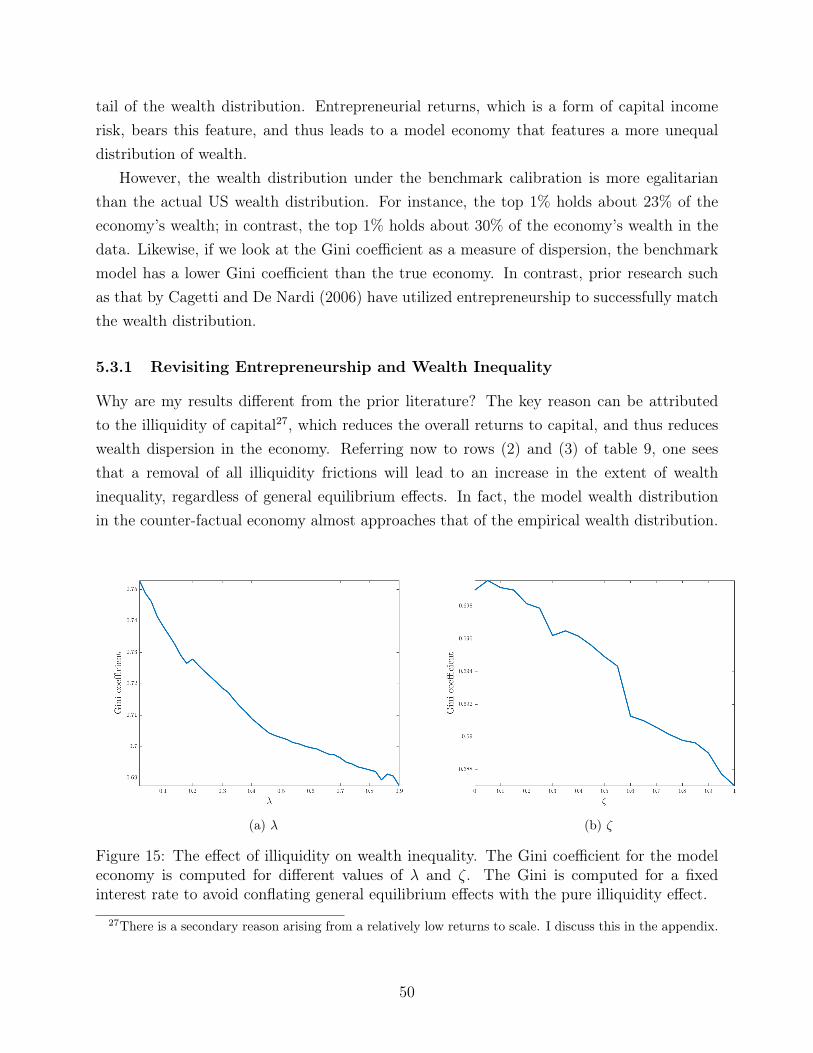
tail of the wealth distribution. Entrepreneurial returns, which is a form of capital incomerisk, bears this feature, and thus leads to a model economy that features a more unequaldistribution of wealth.

However, the wealth distribution under the benchmark calibration is more egalitarianthan the actual US wealth distribution. For instance, the top 1% holds about 23% of theeconomy’s wealth; in contrast, the top 1% holds about 30% of the economy’s wealth in thedata. Likewise, if we look at the Gini coefficient as a measure of dispersion, the benchmarkmodel has a lower Gini coefficient than the true economy. In contrast, prior research suchas that by Cagetti and De Nardi (2006) have utilized entrepreneurship to successfully matchthe wealth distribution.

5.3.1 Revisiting Entrepreneurship and Wealth Inequality

Why are my results different from the prior literature? The key reason can be attributedto the illiquidity of capital27, which reduces the overall returns to capital, and thus reduceswealth dispersion in the economy. Referring now to rows (2) and (3) of table 9, one seesthat a removal of all illiquidity frictions will lead to an increase in the extent of wealthinequality, regardless of general equilibrium effects. In fact, the model wealth distributionin the counter-factual economy almost approaches that of the empirical wealth distribution.

(a) λ (b) ζ

Figure 15: The effect of illiquidity on wealth inequality. The Gini coefficient for the modeleconomy is computed for different values of λ and ζ. The Gini is computed for a fixedinterest rate to avoid conflating general equilibrium effects with the pure illiquidity effect.

27There is a secondary reason arising from a relatively low returns to scale. I discuss this in the appendix.

50

How does capital illiquidity affect returns to investment?Firstly, the transaction costs directly impact investment returns by simply increasing the

user cost of capital. Since every entrepreneur has a non-zero probability of exit, this impliesthat the user cost of capital is larger than the depreciation rate. Consequently, the net returnto investment decreases.

Secondly, recall that in section 5.1.1, I showed that the higher transaction costs leadentrepreneur to operate smaller than optimal firm sizes (if they are investing); moreover,they devote a larger portion of their portfolio to buying bonds. This diminishes the abilityof the entrepreneur to accumulate wealth. Smaller firm sizes mean that the entrepreneur ismaking less business income than she could have; while a larger liquid asset stock meansthat the entrepreneur could strictly be better off moving some bonds into his firm. The grossreturn on asset, which is zf(k, l) + rb, is thus lower.

Finally, section 5.1.1 also showed that many entrepreneurs are operating larger thanoptimal firm sizes. Just as when firms are too small, firm sizes that are too larger alsoreduce the gross return on asset. In this case, the entrepreneur could be strictly better offtransferring her firm’s assets into bonds.

The combined effect leads entrepreneurs to earn lower lifetime incomes when capital ismore illiquid, due to the depressed average returns to capital. As a result, the overall incomedistribution becomes more compressed, and overall wealth dispersion falls. This result isreflected in figure 15, where we see that the Gini coefficient increases as capital becomesmore liquid (i.e. as λ or ζ decreases).

The results here show that, while entrepreneurship does improve the model fit of anotherwise standard incomplete markets model to the wealth distribution, it does not fullygenerate the stark wealth dispersion observed in the data. The finding stands in contrastto the prior literature, which often report exceedingly good model fit to the wealth distri-bution when entrepreneurship is modeled in a Bewley-Huggett-Aiyagari framework. Oneof the key differences between my model, and the preceding literature, is that none of thepreceding research has considered illiquidity as an element affecting entrepreneurial invest-ment dynamics. The findings in this paper therefore suggest that macroeconomic modelsof entrepreneurship that ignore illiquidity might be in fact over-stating the contribution ofentrepreneurial investment to the dispersion of wealth in the data.

5.3.2 Frictions and the distribution of wealth and capital

As discussed earlier, capital illiquidity leads entrepreneurs to accumulate (relatively) moreliquid assets as a buffer stock of savings. Moreover, this also drives low productivity en-trepreneurs to operate larger-than-optimal businesses due to the options value effect. As a

51

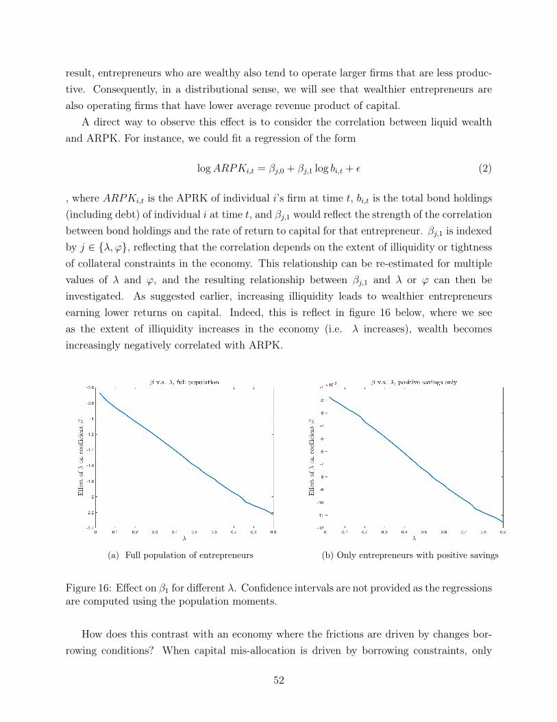
result, entrepreneurs who are wealthy also tend to operate larger firms that are less produc-tive. Consequently, in a distributional sense, we will see that wealthier entrepreneurs arealso operating firms that have lower average revenue product of capital.

A direct way to observe this effect is to consider the correlation between liquid wealthand ARPK. For instance, we could fit a regression of the form

logARPKi,t = βj,0 + βj,1 log bi,t + ε (2)

, where ARPKi,t is the APRK of individual i’s firm at time t, bi,t is the total bond holdings(including debt) of individual i at time t, and βj,1 would reflect the strength of the correlationbetween bond holdings and the rate of return to capital for that entrepreneur. βj,1 is indexedby j ∈ {λ, ϕ}, reflecting that the correlation depends on the extent of illiquidity or tightnessof collateral constraints in the economy. This relationship can be re-estimated for multiplevalues of λ and ϕ, and the resulting relationship between βj,1 and λ or ϕ can then beinvestigated. As suggested earlier, increasing illiquidity leads to wealthier entrepreneursearning lower returns on capital. Indeed, this is reflect in figure 16 below, where we seeas the extent of illiquidity increases in the economy (i.e. λ increases), wealth becomesincreasingly negatively correlated with ARPK.

(a) Full population of entrepreneurs (b) Only entrepreneurs with positive savings

Figure 16: Effect on β1 for different λ. Confidence intervals are not provided as the regressionsare computed using the population moments.

How does this contrast with an economy where the frictions are driven by changes bor-rowing conditions? When capital mis-allocation is driven by borrowing constraints, only

52

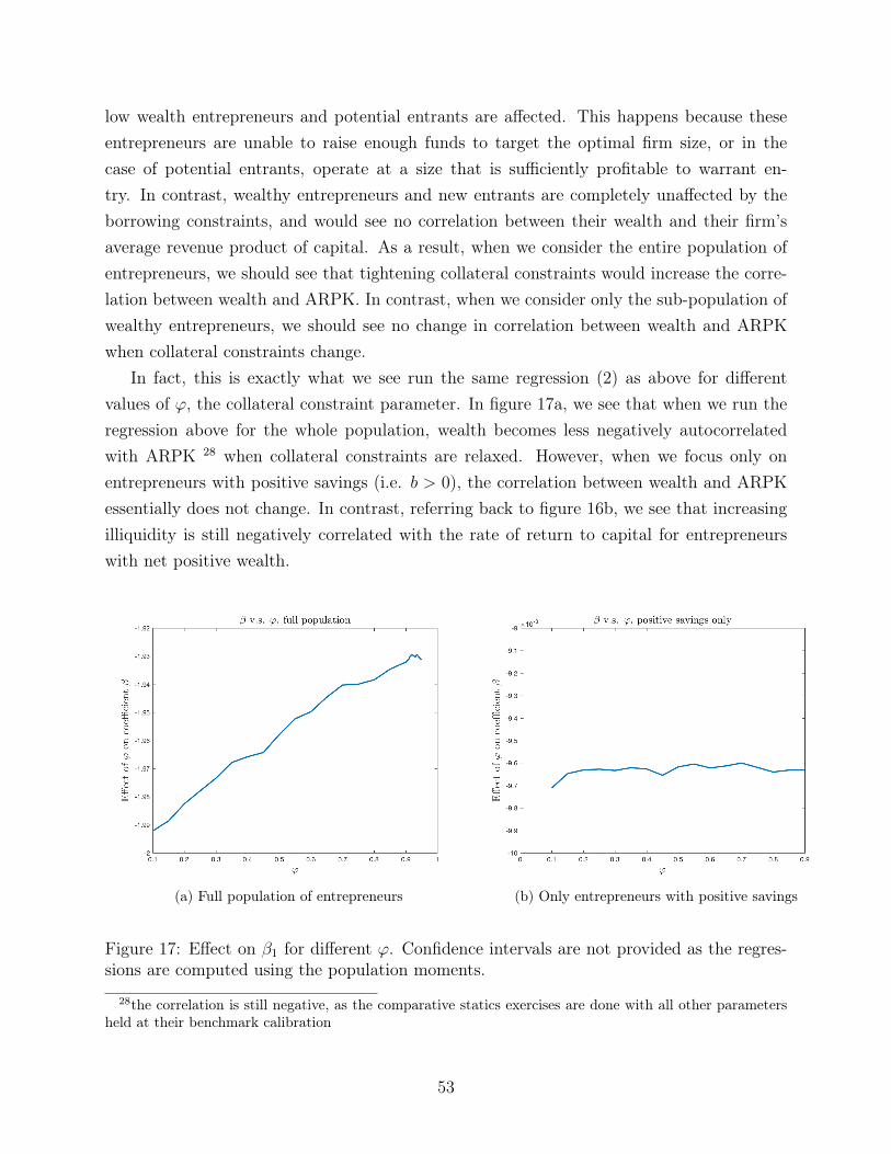
low wealth entrepreneurs and potential entrants are affected. This happens because theseentrepreneurs are unable to raise enough funds to target the optimal firm size, or in thecase of potential entrants, operate at a size that is sufficiently profitable to warrant en-try. In contrast, wealthy entrepreneurs and new entrants are completely unaffected by theborrowing constraints, and would see no correlation between their wealth and their firm’saverage revenue product of capital. As a result, when we consider the entire population ofentrepreneurs, we should see that tightening collateral constraints would increase the corre-lation between wealth and ARPK. In contrast, when we consider only the sub-population ofwealthy entrepreneurs, we should see no change in correlation between wealth and ARPKwhen collateral constraints change.

In fact, this is exactly what we see run the same regression (2) as above for differentvalues of ϕ, the collateral constraint parameter. In figure 17a, we see that when we run theregression above for the whole population, wealth becomes less negatively autocorrelatedwith ARPK 28 when collateral constraints are relaxed. However, when we focus only onentrepreneurs with positive savings (i.e. b > 0), the correlation between wealth and ARPKessentially does not change. In contrast, referring back to figure 16b, we see that increasingilliquidity is still negatively correlated with the rate of return to capital for entrepreneurswith net positive wealth.

(a) Full population of entrepreneurs (b) Only entrepreneurs with positive savings

Figure 17: Effect on β1 for different ϕ. Confidence intervals are not provided as the regres-sions are computed using the population moments.

28the correlation is still negative, as the comparative statics exercises are done with all other parametersheld at their benchmark calibration

53

5.4 Aggregate welfare and productivity

In this section, I discuss the effect of the distortions on two key aggregate outcomes: Welfareand Productivity. Prior to beginning this section, I first provide some definitions to give thereader a consistent reference to the terms I am referring to.

WelfareWelfare here is measured as the consumption equivalent variation between a reference

economy (given by a superscript “R") and the current economy of interest (given by a su-perscript “N"). In particular, for any household i, the consumption equivalent variation µisolves the following problem:

V ((1 + µi)cRi ) = V (cN) (3)

To compute µi for each household, I then simply solve the preceding equation for each pointin the state space S. Given this definition, µi > 0 implies that the household prefers the neweconomy over the reference economy.

Having derive the entire distribution of µi, I then compute aggregate (average) welfareas

µ =

∫µidΛ (4)

Moreover, I am also able to compute welfare changes for subsets of the economy Λs ⊆ Λ.For instance, if I wish to compute the average welfare change for only workers, I can compute

µw =

∫µi × IwdΛ∫

IwdΛ(5)

where Iw is an indicator function that equates to 1 if that household is a worker, and0 otherwise. The denominator is necessary in order to re-normalize the distribution (i.e.compute the conditional average), in order to avoid conflating the changes in the measure ofworkers (which is endogenous) and actual changes in the agent’s welfare (or distribution ofCEV).

Note that the consumption equivalent variation is computed taking into account of thefull transitional dynamics of the economy. I refer the reader to the appendix for a full de-scription of how this is computed.

Aggregate TFP

54

“Aggregate TFP" here refers specifically to the aggregate TFP in the entrepreneur sector.Since the corporate sector is composed of representative firms, there cannot be any TFPlosses with respect to that sector, and hence I choose not to discuss it here29.

Here, my concept of TFP stems from the perspective of a statistician who only observesthe aggregate capital stock, labor input, and output of the entrepreneur sector. In this case,we can derive TFP Z as

Z ≡ Y e

Kαeνe L

(1−αe)νe

(6)

Comparisons of TFP are done across steady-states.

Average productivity of entrepreneurAs the model exhibits endogenous entry and exit, the steady-state distribution of observed

idiosyncratic TFP is different from the underlying distribution of shocks. The selectioneffects can either increase (positive selection) or decrease (negative selection) the averageproductivity of entrepreneurs, and in turn, can have powerful effects on aggregate TFP. Forthis paper, I define the average productivity of an entrepreneur as

Ze =

∫zi × IedΛ∫IedΛ

(7)

where Ie is an indicator function that equates to 1 if that household is an entrepreneur, and0 otherwise.

Comparisons of average productivity are also done across steady-states.Having clarified these definitions, we can now examine the impact of these distortions on

the aggregate economy.

5.4.1 Welfare and productivity

Table 10 reports the aggregate TFP, average productivity of entrepreneurs, and the averagewelfare change for the two asset economy, as well as the counter-factual economy with noresale frictions. Both the PE and GE results are reported for the counter-factual example.The welfare results are reported in terms of percentage consumption equivalent variation.

29This does not mean that the corporate sector is not important in this model. In fact, the amount of(effective) capital allocated to the corporate sector reflects the change in the precautionary savings behaviorof the households, which is an important dimension of this model relative to models of complete markets

55

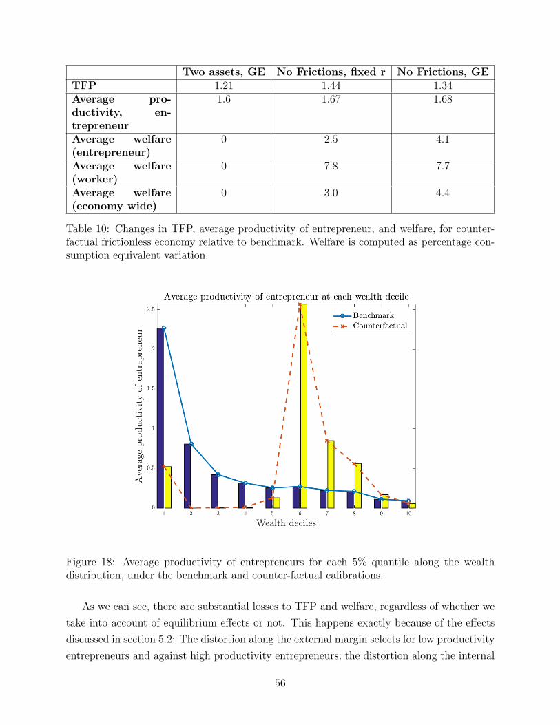
Two assets, GE No Frictions, fixed r No Frictions, GETFP 1.21 1.44 1.34Average pro-ductivity, en-trepreneur

1.6 1.67 1.68

Average welfare(entrepreneur)

0 2.5 4.1

Average welfare(worker)

0 7.8 7.7

Average welfare(economy wide)

0 3.0 4.4

Table 10: Changes in TFP, average productivity of entrepreneur, and welfare, for counter-factual frictionless economy relative to benchmark. Welfare is computed as percentage con-sumption equivalent variation.

Figure 18: Average productivity of entrepreneurs for each 5% quantile along the wealthdistribution, under the benchmark and counter-factual calibrations.

As we can see, there are substantial losses to TFP and welfare, regardless of whether wetake into account of equilibrium effects or not. This happens exactly because of the effectsdiscussed in section 5.2: The distortion along the external margin selects for low productivityentrepreneurs and against high productivity entrepreneurs; the distortion along the internal

56

margin leads low productivity entrepreneurs to operate firms that are too large, and highproductivity entrepreneurs to operate firms that are too small. Moreover, it also results inwealthy entrepreneurs who are less productive, as discussed in section 5.3.2 earlier, and alsoreflect in figure 18.

6 Other Implications

6.1 Implications for Finance Literature: Collateral Constraints or

Illiquidity?

Recent research in the entrepreneurship literature has focused extensively on understand-ing the contribution of financing constraints to mis-allocation in entrepreneurial outcomes.At the micro-level, recent research have focused on testing for the existence of collateralconstraints; at the macro-level, recent research have emphasized a collateralized borrowingchannel to explain the propagation of credit shocks to capital or labor markets. In thissection, I explain how my findings relate to this literature.

To begin the discussion, first consider two scenarios: (A) The economy suffers a negativetemporary shock to the collateral constraint parameter, such that ϕ falls to ϕ′ for one periodbefore recovering; (B) The economy suffers a negative temporary shock to the resale value ofused capital, where λ increases to λ′ for one period before recovering. Scenario A correspondsto a sudden tightening of financial conditions, whereas scenario B corresponds to a suddenfall in the used price of capital. In the case of scenario B, ϕ is readjusted such that the netcollateral constraint is fixed. Like in the earlier counter-factual exercises above, this ensuresthat the extent of financial frictions is held constant, allowing me to isolate the impact offalling resale prices. Figure 19 report the aggregate response of labor hiring, entry and exitrates, and investment, to a 50% decrease in ϕ and a 20% decrease in the resale price ofcapital (corresponding to an approximately 9% increase in λ).

The main thing that one notices is the remarkable similarity of the aggregate responsesto a resale price shock and collateral constraint shock. In both cases, hiring, investment andentry rates fall upon impact, and exit rates increases. This finding is important, because thepolicy response to a financing constraint is very different to one where the value of capitalhas fallen. For instance, recent research studying the used capital market have shown thatthe resale price of used capital can be pro-cyclical. As such, this suggests that a portionof the decline in entrepreneurial startup rate or investment over the course of a recessioncan potentially be attributed to a natural response to the decline in the resale price ofcapital. Findings that attribute the decline in entrepreneurial startup or investment solely

57

to financing constraints could therefore be over-estimating the extent to which financialconstraints have tightened. Moreover, simply looking at aggregates such as the startup rate,exit rate or investment is insufficient to help researchers distinguish between the two sourcesof distortion.

Another important point relates to recent research that have attempted to estimate theexistence and impact of financing constraints on entrepreneurial startup and investment,using exogenous regional variations in asset prices as an identifying instrument. In thatliterature, exogenous variations in house prices are often used as a proxy for variations inthe extent of collateralizable assets, with the argument that houses serve as collateral forentrepreneurs who are taking out loans. A concern that this paper raises is that, to the extentthat house prices are correlated with resale capital prices, the correlations detected by thepreceding research might be reflective simply of the illiquidity effect rather than collateralconstraints. Indeed, as figure 19 shows, liquidity shocks to the price of used capital cangenerate decreased economic activity independently of financial shocks.

58

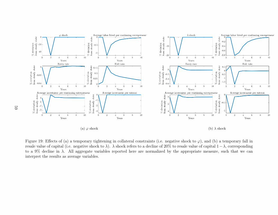
(a) ϕ shock (b) λ shock

Figure 19: Effects of (a) a temporary tightening in collateral constraints (i.e. negative shock to ϕ), and (b) a temporary fall inresale value of capital (i.e. negative shock to λ). λ shock refers to a decline of 20% to resale value of capital 1−λ, correspondingto a 9% decline in λ. All aggregate variables reported here are normalized by the appropriate measure, such that we caninterpret the results as average variables.

59

6.2 Implications for Fiscal Policy

In section 4.1.2, I had discussed the fact that entrepreneurs do not necessarily face tightfinancial constraints arising from limited commitment; rather, the low resale value of cap-ital induces a collateral constraint effect on top of the illiquidity effect. In this section, Ishow using a sketch, an example of how a straightforward policy that reduces the cost ofreallocation can improve welfare and TFP.

In this example, the government commits to a fixed budget G to increase the resale priceof capital from 1 − λ to 1 − λ. In other words, the government commits to paying thedifference λ − λ for every unit of used capital transacted, and the total cost is paid for byG. From the perspective of households, this policy has two benefits: Firstly, it increases theresale value of capital, and therefore reduces the amount of illiquidity risk the individualfaces; secondly, it relaxes the collateral constraint. To finance this policy, the governmenttaxes bond returns. The cost is therefore only borne by relatively wealthier households whohave positive liquid savings.

Using the notation established in section 3, the equilibrium of this model can be definedas follows:

Definition of equilibrium A stationary competitive equilibrium of the model consist ofthe interest rate r, wage rate w, used capital resale price 1 − λ, tax rate τ , value functionsof households and firms {Ve, Vw,Π}, allocations {k′, b′, l} and distribution of agents Λ overthe state space S such that,

1. Taking r, w, 1− λ and τ as given, the households’ and firms’ choices are optimal.

2. The government’s budget, where G is a parameter, balances:

G = τr

∫b× 1{b≥0}dΛ =

(λ− λ

)∫(k′ − (1− δ) k)× I{k′−(1−δ)k<0}dΛ

I{k′−(1−δ)k<0} =

1 , if k′ − (1− δ) k < 0

0 , if k′ − (1− δ) k ≥ 0

3. Markets clear,

(a) Bonds:∫b′dΛ = Kc

(b) Labor:∫θhdΛ =

∫ldΛ + Lc

60

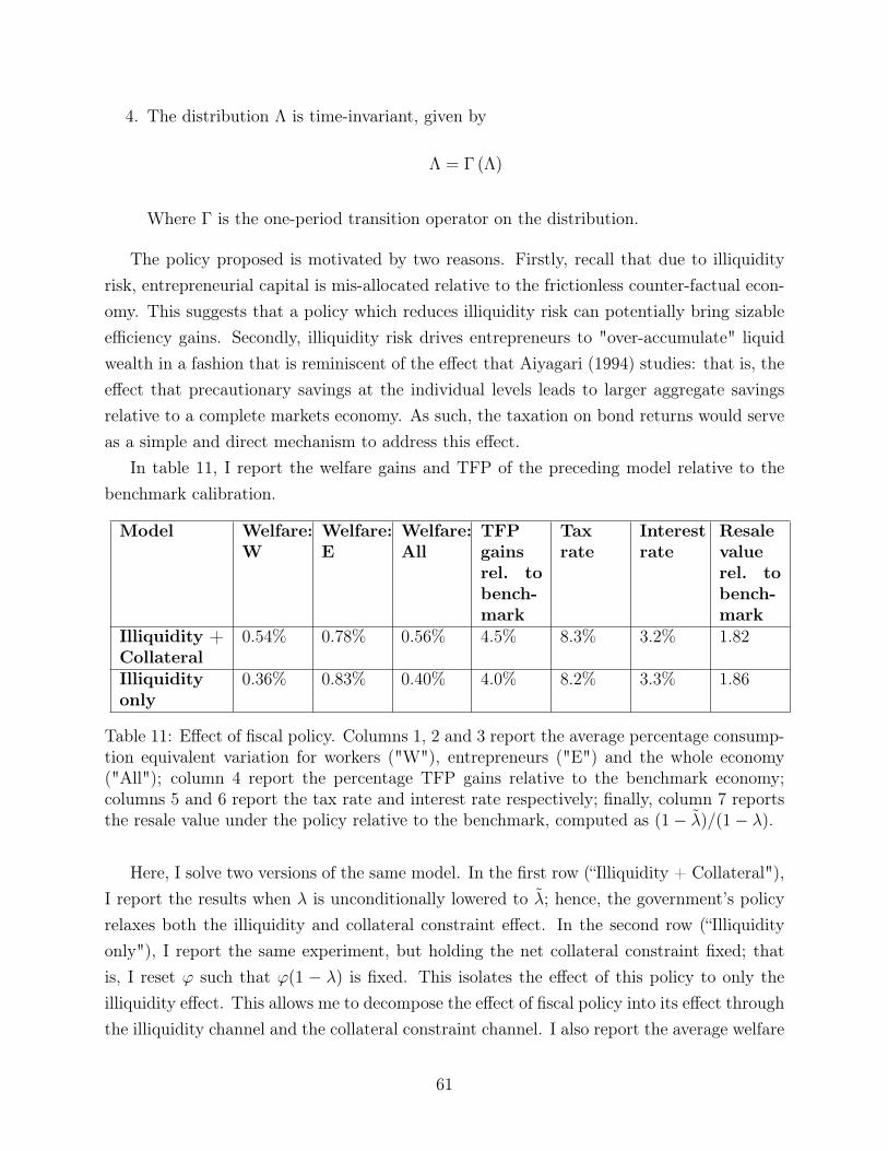
4. The distribution Λ is time-invariant, given by

Λ = Γ (Λ)

Where Γ is the one-period transition operator on the distribution.

The policy proposed is motivated by two reasons. Firstly, recall that due to illiquidityrisk, entrepreneurial capital is mis-allocated relative to the frictionless counter-factual econ-omy. This suggests that a policy which reduces illiquidity risk can potentially bring sizableefficiency gains. Secondly, illiquidity risk drives entrepreneurs to "over-accumulate" liquidwealth in a fashion that is reminiscent of the effect that Aiyagari (1994) studies: that is, theeffect that precautionary savings at the individual levels leads to larger aggregate savingsrelative to a complete markets economy. As such, the taxation on bond returns would serveas a simple and direct mechanism to address this effect.

In table 11, I report the welfare gains and TFP of the preceding model relative to thebenchmark calibration.

Model Welfare:W

Welfare:E

Welfare:All

TFPgainsrel. tobench-mark

Taxrate

Interestrate

Resalevaluerel. tobench-mark

Illiquidity +Collateral

0.54% 0.78% 0.56% 4.5% 8.3% 3.2% 1.82

Illiquidityonly

0.36% 0.83% 0.40% 4.0% 8.2% 3.3% 1.86

Table 11: Effect of fiscal policy. Columns 1, 2 and 3 report the average percentage consump-tion equivalent variation for workers ("W"), entrepreneurs ("E") and the whole economy("All"); column 4 report the percentage TFP gains relative to the benchmark economy;columns 5 and 6 report the tax rate and interest rate respectively; finally, column 7 reportsthe resale value under the policy relative to the benchmark, computed as (1− λ)/(1− λ).

Here, I solve two versions of the same model. In the first row (“Illiquidity + Collateral"),I report the results when λ is unconditionally lowered to λ; hence, the government’s policyrelaxes both the illiquidity and collateral constraint effect. In the second row (“Illiquidityonly"), I report the same experiment, but holding the net collateral constraint fixed; thatis, I reset ϕ such that ϕ(1 − λ) is fixed. This isolates the effect of this policy to only theilliquidity effect. This allows me to decompose the effect of fiscal policy into its effect throughthe illiquidity channel and the collateral constraint channel. I also report the average welfare

61

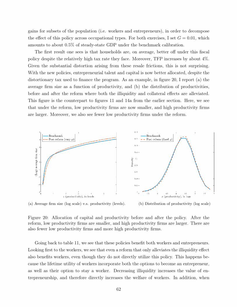
gains for subsets of the population (i.e. workers and entrepreneurs), in order to decomposethe effect of this policy across occupational types. For both exercises, I set G = 0.01, whichamounts to about 0.5% of steady-state GDP under the benchmark calibration.

The first result one sees is that households are, on average, better off under this fiscalpolicy despite the relatively high tax rate they face. Moreover, TFP increases by about 4%.Given the substantial distortion arising from these resale frictions, this is not surprising.With the new policies, entrepreneurial talent and capital is now better allocated, despite thedistortionary tax used to finance the program. As an example, in figure 20, I report (a) theaverage firm size as a function of productivity, and (b) the distribution of productivities,before and after the reform where both the illiquidity and collateral effects are alleviated.This figure is the counterpart to figures 11 and 14a from the earlier section. Here, we seethat under the reform, low productivity firms are now smaller, and high productivity firmsare larger. Moreover, we also see fewer low productivity firms under the reform.

(a) Average firm size (log scale) v.s. productivity (levels). (b) Distribution of productivity (log scale)

Figure 20: Allocation of capital and productivity before and after the policy. After thereform, low productivity firms are smaller, and high productivity firms are larger. There arealso fewer low productivity firms and more high productivity firms.

Going back to table 11, we see that these policies benefit both workers and entrepreneurs.Looking first to the workers, we see that even a reform that only alleviates the illiquidity effectalso benefits workers, even though they do not directly utilize this policy. This happens be-cause the lifetime utility of workers incorporate both the options to become an entrepreneur,as well as their option to stay a worker. Decreasing illiquidity increases the value of en-trepreneurship, and therefore directly increases the welfare of workers. In addition, when

62

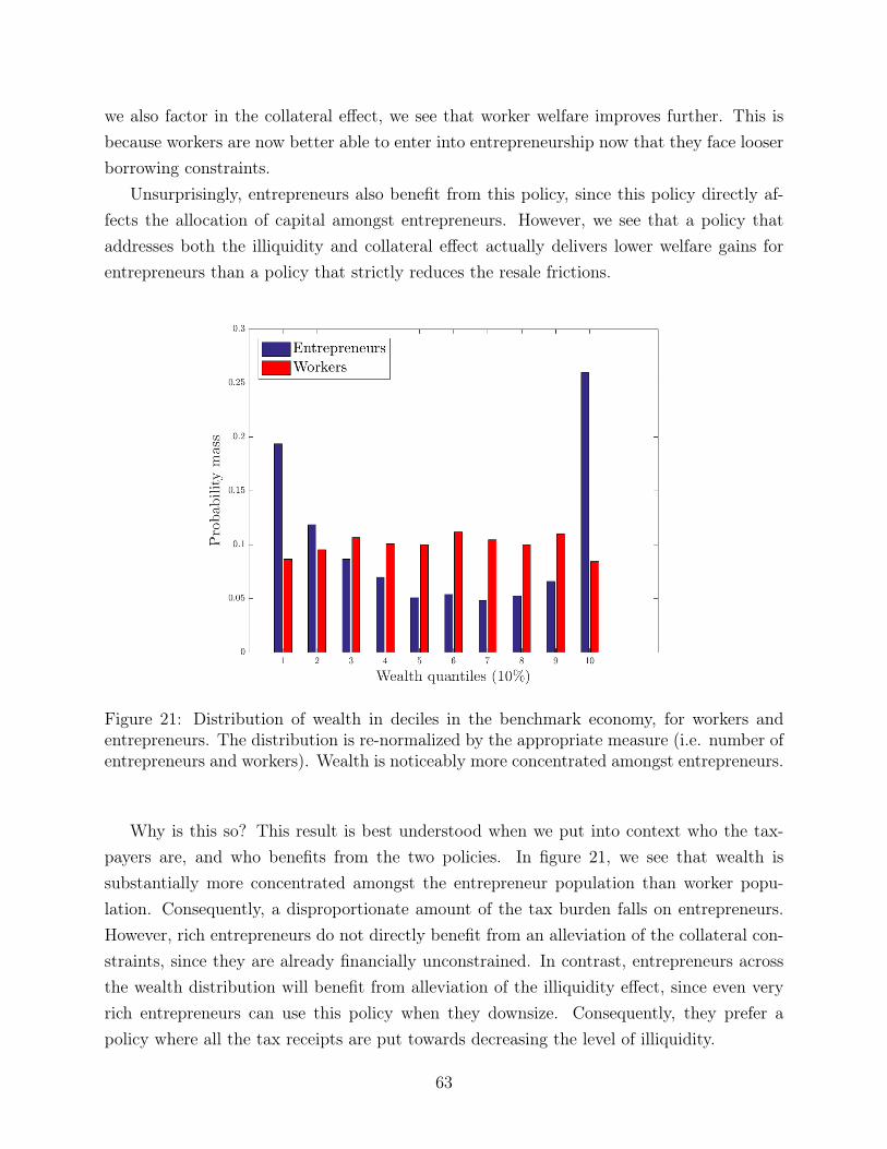
we also factor in the collateral effect, we see that worker welfare improves further. This isbecause workers are now better able to enter into entrepreneurship now that they face looserborrowing constraints.

Unsurprisingly, entrepreneurs also benefit from this policy, since this policy directly af-fects the allocation of capital amongst entrepreneurs. However, we see that a policy thataddresses both the illiquidity and collateral effect actually delivers lower welfare gains forentrepreneurs than a policy that strictly reduces the resale frictions.

Figure 21: Distribution of wealth in deciles in the benchmark economy, for workers andentrepreneurs. The distribution is re-normalized by the appropriate measure (i.e. number ofentrepreneurs and workers). Wealth is noticeably more concentrated amongst entrepreneurs.

Why is this so? This result is best understood when we put into context who the tax-payers are, and who benefits from the two policies. In figure 21, we see that wealth issubstantially more concentrated amongst the entrepreneur population than worker popu-lation. Consequently, a disproportionate amount of the tax burden falls on entrepreneurs.However, rich entrepreneurs do not directly benefit from an alleviation of the collateral con-straints, since they are already financially unconstrained. In contrast, entrepreneurs acrossthe wealth distribution will benefit from alleviation of the illiquidity effect, since even veryrich entrepreneurs can use this policy when they downsize. Consequently, they prefer apolicy where all the tax receipts are put towards decreasing the level of illiquidity.

63

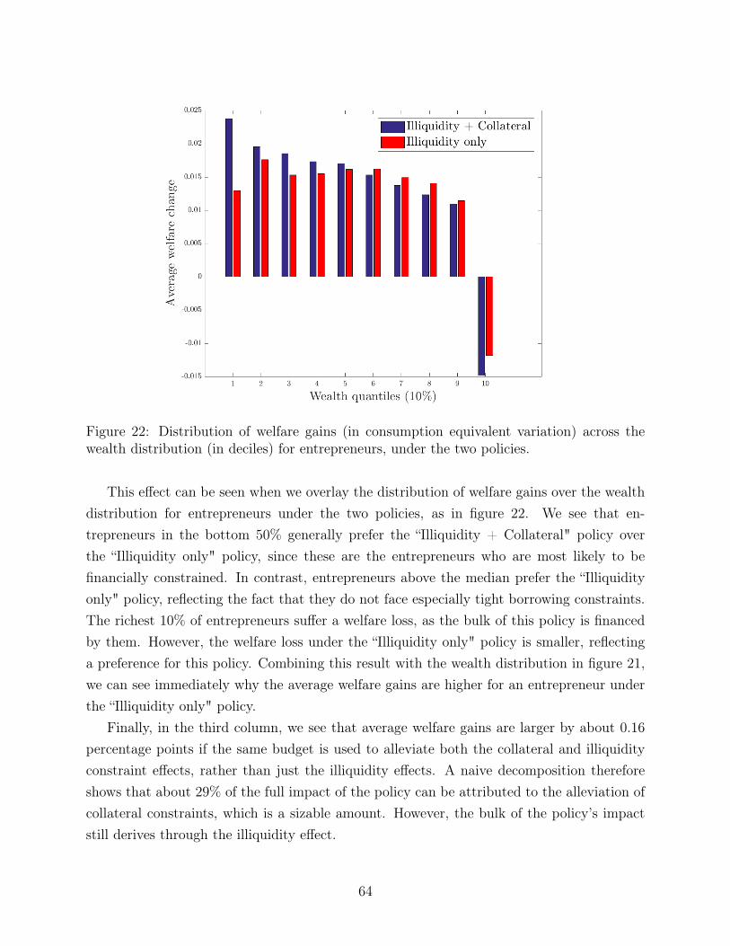
Figure 22: Distribution of welfare gains (in consumption equivalent variation) across thewealth distribution (in deciles) for entrepreneurs, under the two policies.

This effect can be seen when we overlay the distribution of welfare gains over the wealthdistribution for entrepreneurs under the two policies, as in figure 22. We see that en-trepreneurs in the bottom 50% generally prefer the “Illiquidity + Collateral" policy overthe “Illiquidity only" policy, since these are the entrepreneurs who are most likely to befinancially constrained. In contrast, entrepreneurs above the median prefer the “Illiquidityonly" policy, reflecting the fact that they do not face especially tight borrowing constraints.The richest 10% of entrepreneurs suffer a welfare loss, as the bulk of this policy is financedby them. However, the welfare loss under the “Illiquidity only" policy is smaller, reflectinga preference for this policy. Combining this result with the wealth distribution in figure 21,we can see immediately why the average welfare gains are higher for an entrepreneur underthe “Illiquidity only" policy.

Finally, in the third column, we see that average welfare gains are larger by about 0.16percentage points if the same budget is used to alleviate both the collateral and illiquidityconstraint effects, rather than just the illiquidity effects. A naive decomposition thereforeshows that about 29% of the full impact of the policy can be attributed to the alleviation ofcollateral constraints, which is a sizable amount. However, the bulk of the policy’s impactstill derives through the illiquidity effect.

64

7 Conclusion

In this paper, I studied extensively the investment dynamics of entrepreneurs, and its re-lationship with the distribution of wealth, capital, and entrepreneurial productivity. Thereare four key contributions.

The first contribution is to document empirically that the distribution of the rates ofreturn to capital among early stage entrepreneurs, as proxied by the log average revenueproduct of capital, is highly left-skewed. Moreover, entrepreneurs with low rates of returnpersist in this state for longer periods of time than their high return counterparts. Thisobservation runs contrary to the preceding literature on entrepreneurial investment, whichemphasizes collateral constraints as a key driver of entrepreneurial investment behavior.As discussed in this paper, financing constraints generate right tail skewness and right tailpersistence, which is counter-factual to my empirical findings.

The second contribution of this paper is to build a parsimonious model of entrepreneur-ship to rationalize these findings. Specifically, I show that these facts can be easily reconciledwithin a standard macroeconomic model of entrepreneurship once we explicitly model en-trepreneurial capital as an illiquid asset. When capital is no longer a perfect substitute forbonds, poor performing entrepreneurs hold on to capital for extended periods of time due toa real options value effect. At the aggregate level, this manifests as a left skewed distributionof returns to capital, as well as a left tail persistence.

The third contribution of this paper is to connect entrepreneurial investment, and thedispersion in returns to capital, back to the wealth distribution. This paper finds twoimportant results that deviate from the prior literature. When entrepreneurial capital isilliquid, the average returns to wealth is lowered for all households. Consequently, theresulting wealth distribution features lower wealth inequality than which has been reportedin the prior literature. Moreover, wealth dispersion in my model arises in part from a mis-allocation of capital. Relative to a counter-factual economy where capital is fully liquid,there are substantially more poor performing wealthy entrepreneurs. This leads to welfareand TFP losses relative to the counter-factual economy.

The last contribution relates to fiscal policy. Here, I show that a government programthat subsidizes the sale of entrepreneurial capital can substantially improve welfare and TFP.Moreover, this program is fully funded by a tax on liquid bond returns, suggesting that areallocation of wealth can bring about important welfare benefits.

65

References

[1] Philippe Aghion, Ufuk Akcigit, Antonin Bergeaud, Richard Blundell, and David He-mous. Innovation and top income inequality. 2016.

[2] S. Rao Aiyagari. Uninsured idiosyncratic risk and aggregate saving. The QuarterlyJournal of Economics, 1994.

[3] George-Marios Angeletos. Uninsured idiosyncratic investment risk and aggregate saving.Review of Economic Dynamics, 10:1–30, 2007.

[4] Laurent Bach, Laurent E. Calvet, and Paoloo Sodini. Rich pickings? risk, return, andskill in the portfolios of the wealth. July 2016.

[5] Jess Benhabib and Alberto Bisin. Skewed wealth distributions: Theory and empirics.

[6] Jess Benhabib, Alberto Bisin, and Shenghao Zhu. The wealth distribution in bewleymodels with investment risk. Journal of Economic Theory, 2015.

[7] David Berger and Joseph Vavra. Consumption dynamics during recessions. Economet-rica, 83(1), January 2015.

[8] Radim Bohacek. Financial constraints and entrepreneurial investment. Journal of Mon-etary Economics, 2006.

[9] Francisco J Buera, Joseph P. Kaboski, and Yongseok Shin. Finance and development:A tale of two sectors. American Economic Review, 101, August 2011.

[10] Macro Cagetti and Mariacristina DeNardi. Estate taxation, entrepreneurship, andwealth. American Economic Review, 99(1):85–111, 2009.

[11] Marco Cagetti and Mariacristina De Nardi. Entrepreneurship, frictions, and wealth.Journal of Political Economy, 114(5), 2006.

[12] Andrea Caggese. Financing constraints. irreversibility, and investment dynamics. Jour-nal of Monetary Economics, 54:2102–2130, December 2007.

[13] Ana Castaneda, Javier Diaz-Gimenez, and Jose-Victor Rios-Rull. Accounting for theu.s. earnings and wealth inequality. Journal of Political Economy, 2003.

[14] Sagiri Kitao Conesa, Juan Carlos and Dirk Krueger. Taxing capital? not a bad ideaafter all! American Economic Review, 2009.

66

[15] Russell W. Cooper and John C. Haltiwanger. On the nature of capital adjustment costs.The Review of Economic Studies, 73(3):611–633, July 2006.

[16] Francisco Covas. Uninsured idiosyncratic production risk with borrowing constraints.Journal of Economic Dynamics and Control, 2006.

[17] Marco Cozzi. Risk aversion heterogeneity, risky jobs and wealth inequality. October2014.

[18] Steven J. Davis, John Haltiwanger, Kyle Handley, Ron Jarmin, Josh Lerner, andJavier Miranda. Private equity, jobs, and productivity. American Economic Review,104(12):3956–3990, 2014.

[19] Andreas Fagereng, Luigi Guiso, Davide Malacrino, and Luigi Pistaferri. Heterogeneityand persistence in returns to wealth. November 2016.

[20] Douglas Holtz-Eakin, Harvey S. Rosen, and Robert Weathers. Horatio alger meets themobility tables. Small Business Economics, 2000.

[21] Chang-Tai Hsieh and Peter J. Klenow. Misallocation and manufacturing tfp in chinaand india. The Quarterly Journal of Economics, 2009.

[22] Eric Hurst and Annamaria Lusardi. Liquidity constraints, household wealth, and en-trepreneurship. Journal of Political Economy, 112(2):319–347, 2004.

[23] Eric Hurst and Benjamin Pugsley. Wealth, tastes, and entrepreneurial choice. October2015.

[24] Erik Hurst, Annamaria Lusardi, Arthur Kennickell, and Francisco Torralba. The im-portance of business owners in assessing the size of precautionary savings. The Reviewof Economics and Statistics, 92(1):61–69, February 2010.

[25] Greg Kaplan and Giovanni L. Violante. A model of the consumption response to fiscalstimulus payments. Econometrica, 2014.

[26] Fabian Kindermann and Dirk Krueger. High marginal tax rates on the top 1model withidiosyncratic income risk. Working paper, 2015.

[27] Sigiri Kitao. Entrepreneurship, taxation and capital investment. Review of EconomicDynamics, 11:44–69, 2008.

[28] Per Krusell and Anthony A. Smith. Income and wealth heterogeneity in the macroe-conomy. Journal of Political Economy, 106(5), 1998.

67

[29] Moritz Kuhn and Jose-Victor Rios-Rull. 2013 update on the u.s. earnings, income,and wealth distributional facts: A view from macroeconomics 2013 update on the u.s.earnings, income, and wealth distributional facts: A view from macroeconomics. FederalReserve Bank of Minneapolis, Quarterly, (April), 2016.

[30] Andrea Lanteri. The market for used capital. 2016.

[31] Wenli Li. Entrepreneurship and government subsidies: A general equilibrium analysis.Journal of Economic Dynamics and Control, 2002.

[32] Cesaire Meh. Entrepreneurship, wealth inequality, and taxation. Review of EconomicDynamics, 2005.

[33] Benjamin Moll. Productivity losses from financial frictions: Can self-financing undocapital misallocation? American Economic Review, 104(10):3186–3221, 2014.

[34] Ramana Nanda. Entrepreneurship and the discipline of external finance. Mar 2011.

[35] Mariacristina De Nardi and Guilio Fella. Savings and wealth inequality. CEPR discus-sion paper 11746, 2017.

[36] Vasia Panousi. Capital taxation with entrepreneurial risk. 2012.

[37] Benjamin Pugsley and Aysegul Sahin. Grown-up business cycles. September 2015.

[38] Vincenzo Quadrini. Entrepreneurship, saving, and social mobility. Review of EconomicDynamics, 3:1–40, 2000.

[39] Vincenzo Quadrini. Entrepreneurship in macroeconomics. Annals of Finance, 2009.

[40] Emmanuel Saez and Gabriel Zucman. Wealth inequality in the united states since 1913:Evidence from capitalized income tax data. October 2014.

[41] Immo Schott. Start-ups, house prices, and the us recovery. September 2015.

[42] Chong Wang, Neng Wang, and Jinqiang Yang. A unified model of entrepreneurshipdynamics. Journal of Financial Economics, 106:1–23, May 2012.

68

Appendix

I Data appendix I: Data construction

Following the literature, my key strategy is to document key moments for two measures offirm investment: The average revenue product of capital, and the investment rate. Thissection details how these two measures are constructed

I.a Capital stock

In order to construct the average revenue product of capital, I first need to construct thecapital stock of the firm. The KFS provides the researcher the balance sheet of the firm, andit provides a breakdown of the type of capital asset that the entrepreneurial firm owns30.

However, as in most standard models, I consider only a single generic capital asset ofinterest. As such, in order render the results comparable, I construct a representative singleasset, real capital stock, Ki,t, using the nominal value of capital assets as follows:

Ki,t =∑s

Ki,s,t

Ps,t

where Ps,t is the relative price of each capital type s and vintage t. Subscript i indexesthe firm. The relative prices are taken from the BEA. For the aggregated capital stock, Ionly consider the firm’s holdings of product inventories, land and buildings and structures,vehicles, equipment or machinery, and other properties.

I.b Revenue and Value Added

Construction of the average revenue product of capital also necessitates the construction of ameasure of the firm’s real value added. A two step adjustment is used to transform nominalrevenue into real value added. The first step is straightforward; nominal revenue is deflatedby the GDP deflator to obtain real revenue.

30The full range of asset types are product inventories, land and buildings and structures, vehicles, equip-ment or machinery, other properties, cash, and “others".

69

Unfortunately, constructing real value added from real revenue is less straightforward.The KFS does not provide information on the firm’s material expenses; consequently, onecannot simply subtract out the material cost to retrieve value added.

Instead, following the literature, I assume that the firm revenue production function isgiven by a Cobb-Douglas function of the form

Y Ri,j,t = zi,j,tK

βjki,j,tL

βjli,j,tM

βjmi,j,t

where i indexes a firm, j indexes the industry, and t indexes time. z here refers toaggregated TPFR (i.e. it summarizes the firm, industry and aggregate level shocks). Thecapital (K), labor (L) and material (M) intensity parameters (βjk, β

jl , β

jm respectively) are

allowed to vary across industries, but are restricted to sum to unity.Let P j

m denote the cost of materials for industry j. Then value added is

Yi,j,t = Y Ri,j,t − P j

mMi,j,t

As the KFS does not provide information on P jmMi,j,t, the goal is to infer P j

mMi,j,t.To do so, I follow the preceding literature by assuming that capital is fixed one period in

advanced, but the firm is able to adjust it’s labor and material inputs contemporaneously31.Given this, the firm’s optimal material choice will yield the first order condition:

P jm = βjm

Y Ri,j,t

Mi,j,t

=⇒ Yi,j,t = (1− βjm)× Y Ri,j,t

Therefore, given the material share parameter, we can immediately back out value added.For the purposes of this paper, I assume that the entrepreneurial firms have the same materialshare as the industry that they operate in. The material share at the industry level can beestimated directly from national accounting data (the NIPA KLEMS tables). Denoting theestimated material share as βjm, I back out an estimate of value added as32

Yi,j,t = (1− βjm)× Y Ri,j,t

For the rest of this paper, revenue refers to this measure of value added, unless explicitly31See for instance, Olley and Pakes (1996)32One might justifiably be concerned that this measurement of value added is very noisy, and introduces

extra measurement error. As a robustness check, I repeat the empirical exercises using the “raw" revenuemeasure. The qualitative results obtained using the value added measure is replicated when I use the rawrevenue measure.

70

stated otherwise.

I.c Average Revenue Product of Capital

Having constructed both capital and revenue, the (log) average revenue product of capitalis simply

logARPK ≡ log

(Yit

Ki,t−1

)t indicates the survey year. This timing convention is adopted as the KFS only surveys

the firm at the start of the following year for information regarding the current year. Thatis to say, if the survey report is for the year 2004, it was in fact surveyed in 2005. Therefore,K2004 is in fact the end of period capital stock, while Y2004 is the revenue for 2004. Theconvention chosen here hence matches the standard timing convention to construct averageproducts of capital as the ratio of the total revenue to the start of period capital stock.

For the main body of the paper, the moments I report are constructed using a pooledmeasure of logARPK. In practice, moments constructed using pooled logARPK might notbe a good measure since there is likely to be large heterogeneity in capital share and returnsto scale across industries 33. However, due to the small sample size of the KFS relative tothe number of industries34, there is simply insufficient statistical power to draw any usefulinference if one restricted analysis only to the 6 digit NAICS industry level. Instead, Iaddress this issue through two methods.

Residualized ARPK All the benchmark empirical results utilize a residualized measureof logARPK rather than the raw measure. Here, the pooled logARPK variables are resid-ualized by regressing the raw logARPK on two digit NAICS industry level fixed effectsand time dummies. The residuals of this regression then form my measure of logARPK

for analysis. This avoids the issue where permanent differences across industries (such asheterogeneity in capital share and returns to scale) would distort the distribution, and thusintroduce spurious correlations and moments. Moreover, it also removes some of the commonaggregate shocks that might distort the distribution of logARPK over time. The resultspresented in the following sub-sections are constructed using this residualized measure35.

33See for instance, Burnside (1993), who estimates the returns to scale for different industries in the UnitedStates

34There were 3140 firms in 2004 when the survey started; by 2011, there were only 1630 firms left. Incontrast, there are 659 six digit level NAICS code industries.

35As a robustness check, I also construct extended residualized measures of logARPK by using moreregressors that could potentially systematically distort the distribution of logARPK (for instance, the legal

71

Industry level moments The biggest concern about my findings relate to the fact thatthere is substantial permanent heterogeneity across industries that the residualization pro-cess is unable to fully purged. To address these concerns, I also directly investigate therelevant moments at the two digit industry level. Due to the smaller sample size, only oneindustry showed statistically significant results; however, most industries showed economi-cally significant results. Moreover, the qualitative findings at the aggregate level also holdsbroadly across industries. The results at the industry level are reported in this appendix.

I.d Investment rates

To construct investment and investment rates, I use the perpetual inventory method asfollows:

Ii,s,t =Ki,s,t

Ps,t− (1− δs)

Ki,s,t−1

Ps,t−1

Ii,s,t =∑s

Ki,s,t−1∑sKi,s,t−1

Ii,s,t

ii,s,t =Ii,t

Ki,t−1

where Ii,s,t refers to investment levels of firm i for capital type s and vintage t. I allow fordepreciation of each type of capital (δs) to differ according to the BEA depreciation schedule.Gross investment at the firm level is then constructed as a weighted average of the firm’sinvestment for each capital type. Investment rate is then constructed by scaling the grossinvestment by the total lagged capital stock.

Just as in the case of logARPK, using iit “as is” poses a potential problem that the invest-ment series is biased by unobserved aggregate shocks that are orthogonal to the idiosyncraticshocks or frictions that I am interested in studying. To purge the effect of aggregate shockson investment, I construct a residualized investment series by regressing investment rates onyear and two digit NAICS code fixed effects, and construct the relevant investment momentsusing the residuals.

II Data appendix II: Robustness checks

In this section, in an effort to ensure the robustness of my empirical findings, I re-examinethe data moments I reported through multiple cuts of the data.

form of the firm, or the gender of the primary owner of the firm). I find that my benchmark results arerobust to alternative measures. Results computed using these extended measures are available upon request.

72

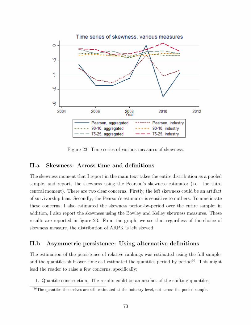
Figure 23: Time series of various measures of skewness.

II.a Skewness: Across time and definitions

The skewness moment that I report in the main text takes the entire distribution as a pooledsample, and reports the skewness using the Pearson’s skewness estimator (i.e. the thirdcentral moment). There are two clear concerns. Firstly, the left skewness could be an artifactof survivorship bias. Secondly, the Pearson’s estimator is sensitive to outliers. To amelioratethese concerns, I also estimated the skewness period-by-period over the entire sample; inaddition, I also report the skewness using the Bowley and Kelley skewness measures. Theseresults are reported in figure 23. From the graph, we see that regardless of the choice ofskewness measure, the distribution of ARPK is left skewed.

II.b Asymmetric persistence: Using alternative definitions

The estimation of the persistence of relative rankings was estimated using the full sample,and the quantiles shift over time as I estimated the quantiles period-by-period36. This mightlead the reader to raise a few concerns, specifically:

1. Quantile construction. The results could be an artifact of the shifting quantiles.36The quantiles themselves are still estimated at the industry level, not across the pooled sample.

73

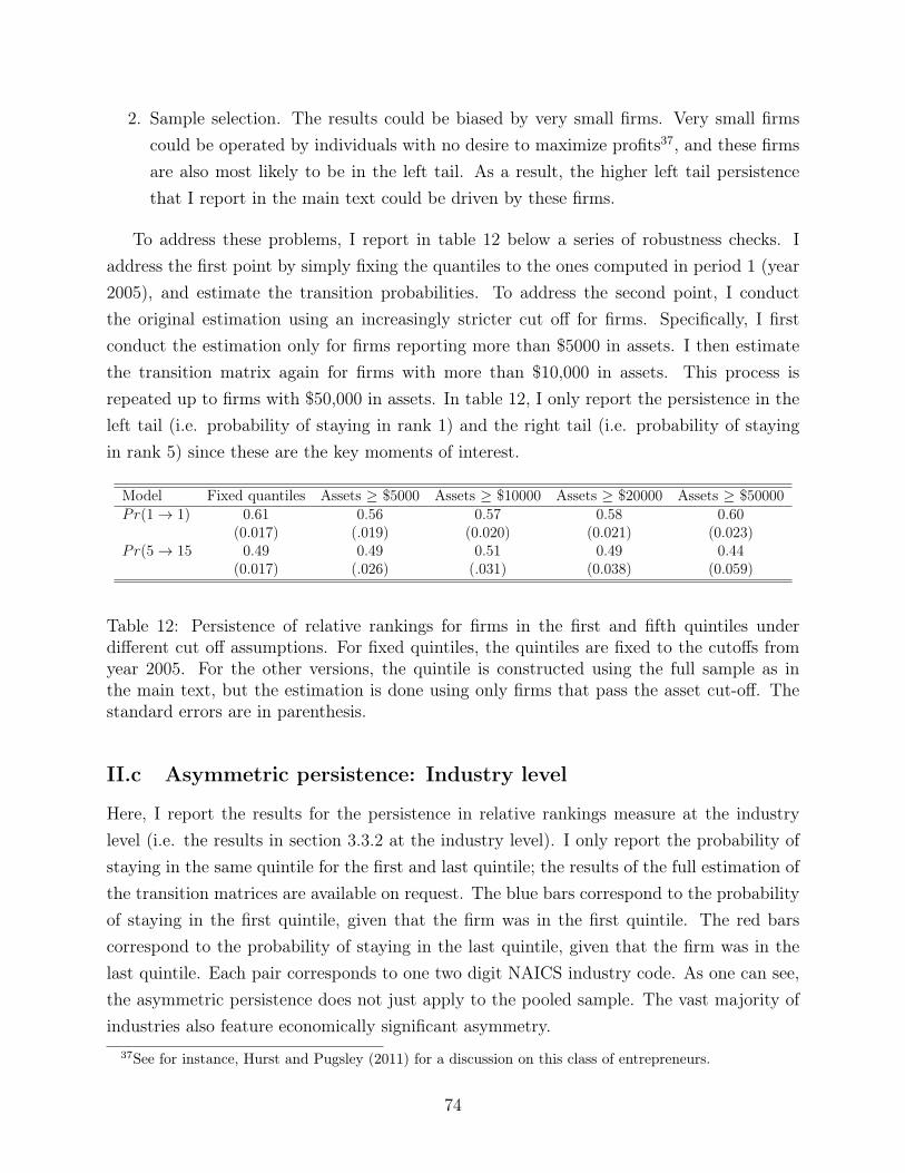
2. Sample selection. The results could be biased by very small firms. Very small firmscould be operated by individuals with no desire to maximize profits37, and these firmsare also most likely to be in the left tail. As a result, the higher left tail persistencethat I report in the main text could be driven by these firms.

To address these problems, I report in table 12 below a series of robustness checks. Iaddress the first point by simply fixing the quantiles to the ones computed in period 1 (year2005), and estimate the transition probabilities. To address the second point, I conductthe original estimation using an increasingly stricter cut off for firms. Specifically, I firstconduct the estimation only for firms reporting more than $5000 in assets. I then estimatethe transition matrix again for firms with more than $10,000 in assets. This process isrepeated up to firms with $50,000 in assets. In table 12, I only report the persistence in theleft tail (i.e. probability of staying in rank 1) and the right tail (i.e. probability of stayingin rank 5) since these are the key moments of interest.

Model Fixed quantiles Assets ≥ $5000 Assets ≥ $10000 Assets ≥ $20000 Assets ≥ $50000Pr(1→ 1) 0.61 0.56 0.57 0.58 0.60

(0.017) (.019) (0.020) (0.021) (0.023)Pr(5→ 15 0.49 0.49 0.51 0.49 0.44

(0.017) (.026) (.031) (0.038) (0.059)

Table 12: Persistence of relative rankings for firms in the first and fifth quintiles underdifferent cut off assumptions. For fixed quintiles, the quintiles are fixed to the cutoffs fromyear 2005. For the other versions, the quintile is constructed using the full sample as inthe main text, but the estimation is done using only firms that pass the asset cut-off. Thestandard errors are in parenthesis.

II.c Asymmetric persistence: Industry level

Here, I report the results for the persistence in relative rankings measure at the industrylevel (i.e. the results in section 3.3.2 at the industry level). I only report the probability ofstaying in the same quintile for the first and last quintile; the results of the full estimation ofthe transition matrices are available on request. The blue bars correspond to the probabilityof staying in the first quintile, given that the firm was in the first quintile. The red barscorrespond to the probability of staying in the last quintile, given that the firm was in thelast quintile. Each pair corresponds to one two digit NAICS industry code. As one can see,the asymmetric persistence does not just apply to the pooled sample. The vast majority ofindustries also feature economically significant asymmetry.

37See for instance, Hurst and Pugsley (2011) for a discussion on this class of entrepreneurs.

74

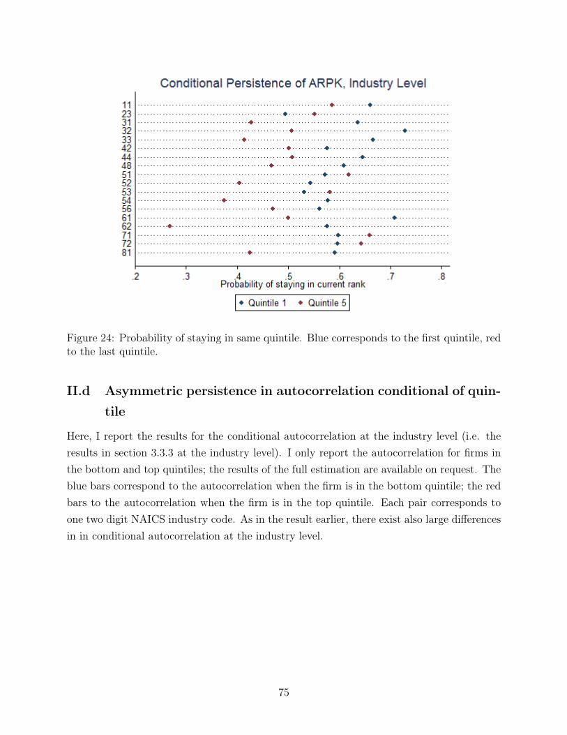
Figure 24: Probability of staying in same quintile. Blue corresponds to the first quintile, redto the last quintile.

II.d Asymmetric persistence in autocorrelation conditional of quin-

tile

Here, I report the results for the conditional autocorrelation at the industry level (i.e. theresults in section 3.3.3 at the industry level). I only report the autocorrelation for firms inthe bottom and top quintiles; the results of the full estimation are available on request. Theblue bars correspond to the autocorrelation when the firm is in the bottom quintile; the redbars to the autocorrelation when the firm is in the top quintile. Each pair corresponds toone two digit NAICS industry code. As in the result earlier, there exist also large differencesin in conditional autocorrelation at the industry level.

75

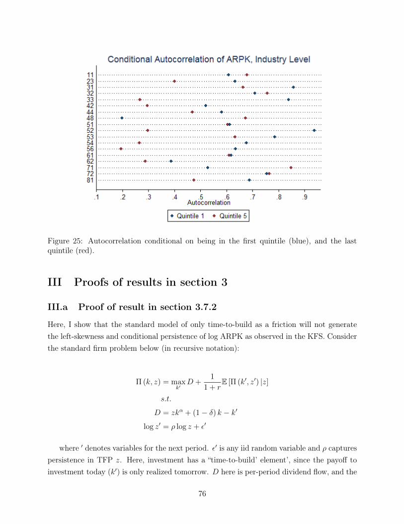
Figure 25: Autocorrelation conditional on being in the first quintile (blue), and the lastquintile (red).

III Proofs of results in section 3

III.a Proof of result in section 3.7.2

Here, I show that the standard model of only time-to-build as a friction will not generatethe left-skewness and conditional persistence of log ARPK as observed in the KFS. Considerthe standard firm problem below (in recursive notation):

Π (k, z) = maxk′

D +1

1 + rE [Π (k′, z′) |z]

s.t.

D = zkα + (1− δ) k − k′

log z′ = ρ log z + ε′

where ′ denotes variables for the next period. ε′ is any iid random variable and ρ capturespersistence in TFP z. Here, investment has a “time-to-build’ element’, since the payoff toinvestment today (k′) is only realized tomorrow. D here is per-period dividend flow, and the

76

firm’s problem is to maximize lifetime dividend flow.The first order condition for capital yields

E[z′(K′)α−1

|z]

=r + δ

α

=⇒ logK ′ =1

α− 1

(log

(r + δ

α

)− logE [z′|z]

)=⇒ logK ′ =

1

α− 1

(log

(r + δ

α

)− ρ log z − logE [exp (ε′) |z]

)⇔ logK =

1

α− 1

(log

(r + δ

α

)− ρ log z−1 − logE [exp (ε) |z−1]

)Where for the second last line, since z′ = zρ exp (ε′), I used the relationship logE [z′|z] =

log (zρE [exp (ε′) |z]) = ρ log z + logE [exp (ε′) |z]. The last line is simply a change of timenotation, with −1 denoting “last period” variables.

Recall that log ARPK is also simply defined as

logARPK = log

(Y

K

)= log z + (α− 1) logK

Combining the two equations, we get

logARPK = log z − ρ log z−1 + log

(r + δ

α

)− logE [exp (ε) |z−1]

Defining ϑ ≡ log(r+δα

)− logE [exp (ε) |z−1], and recalling that log z = ρ log z−1 + ε, we

can simplify the above relation to

logARPK = ρ log z−1 + ε+ log

(r + δ

α

)− ρ log z−1 − logE [exp (ε) |z−1]

= log

(r + δ

α

)− logE [exp (ε) |z−1] + ε

= ϑ+ ε �

As discussed in the main text, the distribution of logARPK simply inherits the distri-bution of ε, scaled by a constant.

77

III.a.1 Skewness

Since the distribution of logARPK is simply the distribution of ε, the skewness of logARPK

will simply be equal to that of ε.

III.a.2 Persistence

Since ε is i.i.d, logARPK is also i.i.d; that is, logARPK exhibits no persistence. Moreover,although the result here is derived for homogeneous parameters, long run differences in α, δor r across industries will not affect the persistence of logARPK.

III.b Proof of result in section 3.7.3

Here, I show that the common static investment framework with limited commitment inborrowing will not allow the model to match the left-skewness of the empirical logARPK

distribution.Consider the following model:

Π (a, z) = maxkD +

1

1 + rE [Π (a′, z′) |z]

s.t.

D = Y − (r + δ)k + (1 + r)a

Y = zkα

k ≤ (1 + ϕ)a

log z′ = ρ log z + ε′

In this framework, there is a financial constraint as firms cannot rent as much capital asthey desire. Instead, they either fully finance using internal assets (a), or they utilize thedebt markets to finance their investments up to ϕ of their assets. ϕ ∈ [0,∞) captures howmuch the individual can leverage on his own wealth. If ϕ = 0, no borrowing is possible; ifϕ→∞, there is no borrowing constraint.

Denote by µ the Lagrange multiplier on the borrowing constraint. The first order condi-tion on capital yields

αY

K= r + δ + µ

=⇒ logARPK = log(r + δ + µ)− log(α)

78

Note that for firms that are unconstrained, µ = 0. Therefore, we see that the supportfor logARPK is given by [log r+δ

α,∞) �.

III.b.1 Skewness

As discussed in the main text, since the distribution is left-truncated, the distribution mustnaturally be right-skewed. This result is independent of the distribution of the underlyinginnovations.

III.b.2 Persistence

The distribution will exhibit greater persistence in the right tail than the left tail. To seethis, consider, at time t, two firms i and j. For firm i, assume that the firm is unconstrained,so µ = 0; consequently, the ARPK of firm i evaluates to

logARPKi,t = log(r + δ)− log(α)

For firm j, assume that the firm is constrained, so µ > 0; consequently, the ARPK of firm j

evaluates to

logARPKj,t = log(r + δ + µj,t)− log(α)

Note that logARPKj > logARPKi; that is, firm j is in the right tail of the distribution,whereas firm i is in the left tail.

The autocorrelation of logARPK for firm i is trivially 0:

corr(logARPKi,t, logARPKi,t+1) = corr (log(r + δ)− log(α), log(r + δ + µi,t+1)− log(α))

= 0

In contrast, for firm j, the autocorrelation is strictly positive:

corr(logARPKj,t, logARPKj,t+1) = corr (log(r + δ + µj,t)− log(α), log(r + δ + µj,t+1)− log(α))

> 0

This holds true trivially because µ is always strictly bigger than 0.Consequently, we see that there is greater persistence in the right tail than the left tail

of the distribution.

79

III.c Proof of result in section 3.7.4

Using the same framework for section 3.7.2, we can extend it with collateralized borrowing,and write the firm’s problem as

Π (b, k, z) = maxk′,b′

Y + (1− δ) k + (1 + r) b− k′ − b′ + 1

1 + rE [Π (b′, k′, z′) |z]

s.t.

Y = zkα

log z′ = ρ log z + ε′

b′ ≥ −ϕk′

Y + (1− δ) k + (1 + r) b ≥ k′ + b′

where b < 0 indicates that the firm is borrowing, and ϕ < 1 in order for the collateralconstraint to be meaningful (if ϕ ≥ 1, then the firm can always borrow enough to hit theoptimal firm size). The last constraint indicates that the firm cannot issue equity. Re-statedin terms of Lagrange multipliers and defining net wealth ω ≡ Y + (1− δ) k + (1 + r) b, weobtain the firm’s problem as

Π (ω, z) = maxk′,b′

ω − k′ − b′ + 1

1 + rE [Π (ω′, z′) |z] + µ (b′ + ϕk′) + κ (ω − k′ − b′)

s.t.

ω′ = z′k′α + (1− δ) k′ + (1 + r) b′

log z′ = ρ log z + ε′

The envelope condition is

∂Π

∂ω= 1 + κ

and the first order conditions for capital and bond are (respectively):

0 = −1 +1

1 + rE[∂Π′

∂ω′

(αz′k

′α−1 + (1− δ))|z]

+ µϕ− κ

0 = −1 +1

1 + rE[∂Π′

∂ω′(1 + r) |z

]+ µ− κ

First, combining the first order conditions for bonds with the envelope conditions, we get

80

0 = −1 +1

1 + rE [(1 + κ′) (1 + r) |z] + µ− κ

=⇒ E [κ′|z] = κ− µ

Next, combining the first order conditions for capital with the envelope conditions, weget

1

1 + rE[(1 + κ′)

(αz′k

′α−1 + (1− δ))|z]

= 1 + κ− µϕ

Next, we can express k′ in terms of the Lagrange multipliers and z. For convenience, I willmove all equations one “time step" back (so ′ variables become “un-primed”, and “un-primed”variables are now −1).

I now re-write the first order conditions for capital as

kα−1 (E [z|z−1] + E [κz|z−1]) =r + δ

α+ (κ−1 − µ−1ϕ)

(1 + r

α

)− E [κ|z−1]

(1− δα

)Next, using the first order conditions for bonds, we note that

(κ−1 − µ−1ϕ)1 + r

α− E [κ|z−1]

(1− δα

)= (κ−1 − µ−1ϕ)

1 + r

α− (κ−1 − µ−1)

(1− δα

)= κ−1

r + δ

α− µ−1

ϕ (1 + r)− 1 + δ

α

=r + δ

α

(κ−1 − µ−1

ϕ (1 + r)− 1 + δ

r + δ

)=r + δ

α(κ−1 − µ−1ϕ)

where ϕ(1+r)−1+δr+δ

≡ ϕ ∈[−1+δr+δ

, 1], as 0 ≤ ϕ ≤ 1. Putting this relationship back into the

first order conditions for capital, we get

kα−1 =

[r + δ

α+r + δ

α(κ−1 − µ−1ϕ)

][E [z|z−1] + E [κz|z−1]]−1

Where we have obtained an implicit solution for k in terms of z and the Lagrange mul-tipliers. Substituting this back into the definition of logARPK,

81

=⇒ logARPK = log z + (α− 1) log k

= log z + log

(r + δ

α+r + δ

α(κ−1 − µ−1ϕ)

)− log (E [z|z−1] + E [κz|z−1])

= log z + log

[(r + δ

α

)(1 + κ−1 − µ−1ϕ)

]− log

[(E [z|z−1])

(1 +

E [κz|z−1]

E [z|z−1]

)]= log z + log

(r + δ

α

)+ log (1 + κ−1 − µ−1ϕ)− logE [z|z−1]− log

(1 +

E [κz|z−1]

E [z|z−1]

)= log z − logE [z|z−1] + log

(r + δ

α

)+ log (1 + κ−1 − µ−1ϕ)− ...

log

(1 +

E [κ|z−1]E [z|z−1] + covz−1 (κ, z)

E [z|z−1]

)= log z − logE [z|z−1] + log

(r + δ

α

)+ log (1 + κ−1 − µ−1ϕ)− ...

log

(1 + E [κ|z−1] +

covz−1 (κ, z)

E [z|z−1]

)= log z − logE [z|z−1] + log

r + δ

α+ log (1 + κ−1 − µ−1ϕ)−

log

(1 + κ−1 − µ−1 +

covz−1 (κ, z)

E [z|z−1]

)Where I went from the second last line to the last line using the first order conditions for

bonds (E [κ|z−1] = κ−1 − µ−1)Finally, noting that

log z − logE [z|z−1] = ρ log z−1 + ε− logE[zρ−1 exp (ε) |z−1

]= ρ log z−1 + ε− ρ log z−1 − logE [exp (ε) |z−1]

= ε− logE [exp (ε) |z−1]

and that under the model of only time-to-build and no collateral constraints,

logARPKTTB = logr + δ

α− logE [exp (ε) |z−1] + ε

We obtain for logARPK:

logARPK = logARPKTTB + log (1 + κ−1 − µ−1ϕ)− log

(1 + κ−1 − µ−1 +

covz−1 (κ, z)

E [z|z−1]

)Now, note that since −1+δ

r+δ≤ ϕ ≤ 1, we see that κ−1 − µ−1ϕ ≥ κ−1 − µ−1. Moreover,

82

since covz−1 (κ, z) < 0 and E [z|z−1] > 0, covz−1 (κ,z)

E[z|z−1]< 0. As such, we see that

log (1 + κ−1 − µ−1ϕ)− log

(1 + κ−1 − µ−1 +

covz−1 (κ, z)

E [z|z−1]

)≡ ξ−1 > 0

where I write ξ−1 to note that this is a pre-determined variable.Rewriting the equation for logARPK again, and defining logARPKTTB ≡ A for nota-

tional ease, we get the following simple linear relation between the “time to build" ARPKand the actual ARPK:

logARPK = A+ ξ−1

�

III.c.1 Skewness

To derive the unconditional skewness of logARPK, note that (and using the notationS (X, Y, Y ) for the co-skewness between X and Y ):

skewness (logARPK) = skewness (A+ ξ−1)

=1

σ3A + σ3

ξ−1

[σ3AS (A) + 3σ2

AσξS (A,A, ξ−1) + 3σAσ2ξS (A, ξ−1, ξ−1) + σ3

ξS (ξ−1)]

Note that while A depends on ε (“today’s innovation”), ξ−1 depends on ε−1 (“yesterday’sinnovation”). As such, A ⊥ ξ−1, which implies that 3σ2

AσξS (A,A, ξ) + 3σAσ2ξS (A, ξ, ξ) = 0:

i.e. they have 0 co-skewness, since they are independent. As such, the skewness of logARPK

reduces to

skewness (logARPK) =1

σ3A + σ3

ξ−1

[σ3AS (A) + σ3

ξS (ξ−1)]

Finally, recall that S (A) = S (ε) (and likewise for the standard deviation); therefore, weobtain the final relation:

skewness (logARPK) =1

σ3ε + σ3

ξ−1

[σ3εS (ε) + σ3

ξS (ξ−1)]

83

Note that if S (ξ−1) > − σ3ε

σ3ξ−1

S (ε), then the distribution will always be right-skewed. This

is trivially true for all S (ε) > 0, since S (ξ−1) > 0 (ξ−1 has a left-truncated distribution sinceit is strictly bigger than 0). Moreover, if S (ξ−1) < − σ3

ε

σ3ξ−1

S (ε), then the skewness of log

ARPK is trivially higher than the skewness of the innovations, although the distribution oflog ARPK will be left-skewed. �

III.c.2 Persistence

Here, I show how the model with collateral constraints produces asymmetric persistence inARPK. To proceed, I first show how there is unconditional autocorrelation, and then showhow this autocorrelation is asymmetric.

Persistence We can compute the autocovariance of logARPK to understand its persis-tence. Specifically,

cov(logARPK, logARPK−1) = cov (A+ ξ−1, A−1 + ξ−2)

= cov (A,A−1) + cov (A, ξ−2) + cov (ξ−1, A−1) + cov (ξ−1, ξ−2)

= cov (ξ−1, A−1) + cov (ξ−1, ξ−2)

> 0

So we see that logARPK exhibits persistence (positive autocorrelation).

Asymmetric Persistence We can now show that the model with collateral constraintsdelivers asymmetric persistence, where the right tail exhibits greater persistence than theleft tail.

To do so, recall that ξ ∈ [0,∞), while A ∈ R. As such, we can always define somearbitrary quantile of the distribution q− such that the following holds:

1. ∀ logARPK < q−, Pr(ξ−1 = 0) = 1 such that logARPK = A

2. ∀ logARPK > 1− q−, Pr(ξ−1 = 0) < 1

Moreover, by the definition of a quantile, Pr(logARPK < q−) = Pr(logARPK >

1− q−).Next, consider 2 types of firms: i and j, where logARPKi < q− and logARPKj > 1−q−.

84

Note that for firm i,

cor(logARPKt, logARPKt+1) = cor(At, At+1) + cor(At, At+1 + ξt)

= cor(At, ξt)

where this correlation term reflects the probability that a firm becomes financially con-strained given it’s productivity shock. This reflects that fact that even for large firms, thereis a non-zero probability that they will become financially constrained.

For firm j,

cor(logARPKt, logARPKt+1) = cor(At + ξt−1, At+1 + ξt)

= cor(At, At+1) + cor(At, ξt) + cor(ξt−1, At+1) + cor(ξt−1, ξt)

= cor(At, ξt) + cor(ξt−1, ξt)

Here, cor(ξt−1, At+1) = 0 since the probability of being financially constrained “yesterday"does not depend on future productivity shocks. However, cor(ξt−1, ξt) > 0 as noted earlier.Therefore, we see that firms of type i exhibit lower autocorrelation than firms of type j. Inother words, the autocorrelation in the right tail of the distribution is greater than that inthe left tail. �

IV Computational Appendix

In this section, I detail in subsection IV.a the solution method used in solving the individual’sproblem, and in subsection IV.b the method used in solving for the stationary equilibrium.A novel contribution to the literature is the algorithm used in solving for the stationaryequilibrium.

IV.a Solving the individual’s problem

The household’s problem is broken down into a multi-stage problem in order to render itnumerically feasible to solve. The steps are detailed below.

IV.a.1 First stage: Occupational choice

Define the intermediate value functions Vee, Vew, Vwe, Vww as the value functions of (1) anentrepreneur who has chosen to stay as an entrepreneur, (2) an entrepreneur who decides toexit, (3) a worker who decides to become an entrepreneur, and (4) a worker who decides to

85

stay a worker; moreover, let this be the value function associated with the household whohas already made its optimal portfolio-savings choice.

Given this definition, we see that the optimal occupational choice of an entrepreneur isgiven by

Ve = maxh′

(1− h′)Vee + h′ × Vew

and the optimal occupational choice of a worker is given by

Vw = maxh′

(1− h′)Vwe + h′ × Vww

where h′ = 1 if the household chooses to become a worker tomorrow, and h′ = 0 if shechooses to become a entrepreneur.

IV.a.2 Second stage: Savings-investment

The investment-savings problem is described for each for the four groups of households below.Here, for convenience, I shall define the interest rate function r ≡ r × 1{b≥0} + rd × 1{b<0}.

Entrepreneur: Exit

For an entrepreneur who decides to exit, her problem is simply

Vew(ψθ, z, k, b

)= max

b′U (c) + βE

[Vw

(ψz′, θ′, b′

)|ψθ]

s.t.

c+ b′ = π∗ + (1 + r) b+ (1− ζ) (1− λ) (1− δ) k

b′ ≥ b

To reduce the dimensionality of this problem, I approximate

Vew(ψθ, b′

)≡ E

[Vw

(ψz′, θ′, b′

)|ψθ]

using a cubic spline in the b′ direction. I then solve the individual’s problem using themonotone condition.

Entrepreneur: Stay

For the entrepreneur who stays an entrepreneur, it is more convenient to define anotherset of intermediate value functions. Let V I

ee, V Dee and V 0

ee denote the value functions of an

86

entrepreneur who has decided to (1) invest in his business, (2) disinvest, and (3) keep thesame capital stock into the next period.

For an investing entrepreneur, his problem is

V Iee

(ψθ, z, k, b

)= max

k′,b′U (c) + βE

[Ve

(ψθ′, z′, k′, b′

)|z]

s.t.

c+ (k′ − (1− δ) k) + b′ + fsk = π∗ + (1 + r) b

k′ > (1− δ) k

b′ ≥ −ϕ (1− λ) (1− δ) k′ − b

For a disinvesting entrepreneur, his problem is

V Dee

(ψθ, z, k, b

)= max

k′,b′U (c) + βE

[Ve

(ψθ′, z′, k′, b′

)|z]

s.t.

c+ (1− λ) (k′ − (1− δ) k) + b′ = π∗ + (1 + r) b

0 < k′ < (1− δ) k

b′ ≥ −ϕ (1− λ) (1− δ) k′ − b

Finally, for an entrepreneur who is holding the same (depreciated) capital stock, hisproblem is

V 0ee

(ψθ, z, k, b

)= max

k′,b′U (c) + βE

[Ve

(ψθ′, z′, k′, b′

)|z]

s.t.

c+ b′ = π∗ + (1 + r) b

k′ = (1− δ) k

b′ ≥ −ϕ (1− λ) (1− δ) k′ − b

This formulation posses three problems. Firstly, the state space spanned by K × B isnot orthogonal due to the financing constraints, which makes standard numerical methodsnot feasible. Secondly, as the portfolio choice here is non-trivial, computational time issubstantially increased. Moreover, due to the asymmetric adjustment cost, the type ofadjustment itself is conditional on the current state of capital holdings. Finally, the statespace of the entrepreneur is spanned by four variables, which also increases computationaltime substantially. To address these issues, I consider the following modifications to the

87

problem.

Orthogonality problem

Firstly, I address the orthogonality problem by defining a new variable, net liquid asset, aas follows:

a ≡ b+ ϕ (1− δ) (1− λ) k + b ≥ 0

The state space of the entrepreneur SE is now defined by(ψθ, z, k, a

)∈ Ψθ×Z×K×A = SE,

which is orthogonal, since both a and k are only restricted by a ≥ 0 and k ≥ 0.Using this new definition, I address the numerical challenges arising from the non-trivial

portfolio choice problem and dimensionality problem using the following strategy.

Portfolio choice and Dimensionality problem

Firstly, note that conditioned on deciding to stay as an entrepreneur (i.e. Vee), the currentsignal shock ψθ is not informative of the next period’s signal as it is IID. As such, the relevantstate space for the entrepreneur who is staying as an entrepreneur is simply the subspaceSEE = Z×K× A ⊂ SE. This cuts down on one dimension.

Secondly, note that because of the IID nature of ψθ, the conditional expectation E[Ve(ψθ′, z′, k′, a′

)|z]

is defined only over the three dimensional subspace SEE. Specifically, we can write the fol-lowing definition:

Vee (z, k′, a′) ≡ E[Ve

(ψθ′, z′, k′, a′

)|z]

To evaluate the continuation value of k′ and a′, I then approximate Ve using a twodimensional cubic spline along the dimensions of k′ and a′.

Thirdly, we can take advantage of the linear separability of the cost function to reducethe dimensionality of the state space. Specifically, note that conditional on either form ofadjustment, we can rewrite the household’s budget as

c+ b′ + k′ + C1 (k′) = π∗ + (1 + r) b+ (1− δ) k − C2 (k)

⇔ c+ a′ − ϕ (1− δ) (1− λ) k′ + k′ + C1 (k′) = π∗ + (1 + r) (a− ϕ (1− δ) (1− λ) k) + (1− δ) k − C2 (k)

where C (k′, k) = C1 (k′) + C2 (k) is the total cost associated with this adjustment.

88

When the firm is adjusting upwards (i.e. investing, denoted henceforth by I), we get

C1 (k′) = 0

C2 (k) = fsk

When the firm is adjusting downwards (i.e. disinvesting, denoted henceforth by D), weget

C1 (k′) = −λk′

C2 (k) = λ (1− δ) k

Therefore, we have two budget constraints given by

c+ a′ − ϕ (1− δ) (1− λ) k′ + k′ = π∗ + (1 + r) a+ (1− δ − fs − (1 + r)ϕ(1− δ)(1− λ)) k ( if I)

c+ a′ + (1− ϕ(1− δ)) (1− λ) k′ = π∗ + (1 + r) a+ (1− (1 + r)ϕ) (1− λ)(1− δ)k ( if D)

Also, note that the budget for no adjustment (i.e. k′ = (1− δ) k) is given by

c+ b′ = π + (1 + r) b

c+ b′ = π + (1 + r)a− (1 + r)ϕ(1− δ) (1− λ) k

⇔ c+ b′ + ϕ(1− δ) (1− λ) k′ − ϕ(1− δ) (1− λ) k′ = π + (1 + r)a− (1 + r)ϕ(1− δ) (1− λ) k

⇔ c+ a′ − ϕ(1− δ) (1− λ) (1− δ) k = π + (1 + r)a− (1 + r)ϕ(1− δ) (1− λ) k

⇔ c+ a′ = π∗ + (1 + r)a− (r + δ)ϕ(1− δ) (1− λ) k

Next, we can define by x the total liquid value of the portfolio. That is, let

xI ≡ π∗ + (1 + r) a+ (1− δ − fs − (1 + r)ϕ(1− δ)(1− λ)) k ( if I)

xD ≡ π∗ + (1 + r) a+ (1− (1 + r)ϕ) (1− λ)(1− δ)k ( if D)

xO ≡ π∗ + (1 + r)a− (r + δ)ϕ(1− δ) (1− λ) k

At this point, it is important to note that because x = x (z, k, a), for any generic (z, k, a)-triple, it is unlikely that xI = xD numerically, due to their differing definitions. However,because this total liquid value is a sufficient state variable for the (z, k, a)-triple, it does notmatter that xI 6= xD for the same generic (z, k, a)-triple.

Now, define by{gaI (x) , gkI (x)

}and

{gaD (x) , gkD (x)

}the optimal unconstrained savings-

investment policy (i.e. choice of a′ and k′) when the household is faced with the budget

89

constraints defined by xI and xD respectively (and V Iee and V D

ee the value functions associatedwith this policy). That is, let them solve the two problems

V Iee = max

gaI ,gkI

U (c) + βE[Ve

(ψθ′, z′, k′, a′

)|z]

s.t.

c+ +gaI + (1− ϕ(1− δ) (1− λ)) gkI = xI

gkI > 0

gaI ≥ 0

and

V Dee = max

gaD,gkD

U (c) + βE[Ve

(ψθ′, z′, k′, a′

)|z]

s.t.

c+ gaD + (1− λ− ϕ(1− δ)(1− λ)) gkD = xD

gkD > 0

gaD ≥ 0

Notice that for this sub-problem, the household does not care about the individual com-ponents of the current portfolio, and only cares about its total value x. Consequently,{gaI (x) , gkI (x)

}and

{gaD (x) , gkD (x)

}are only functions of x.

Finally, let{ga0 , g

k0

}denote the optimal savings policy when the household is not adjust-

ing. In particular gk0 = (1− δ) k.First, for convenience, denote the following indicator functions as follows:

II =

1 (if gkI > (1− δ) k)

0 (otherwise)

ID =

1 (if gkI < (1− δ) k)

0 (otherwise)

Iv =

1 (if V Iee > V D

ee )

0 (otherwise)

I0 =

1 (otherwise)

0 (if V 0ee ≥ max

{V Iee, V

Dee

}

90

Now, denote by ga(ψθ′, z, k, a

)and gk

(ψθ′, z, k, a

)the optimal constrained savings-investment

policy functions. They must satisfy the following condition: For any portfolio state (z, k, a)38, we have:[

ga

gk

]=

[II × Iv ×

[gaIgkI

]◦(xI)

+ ID × (1− Iv)×

[gaDgkD

]◦(xD)]

+

(1− I0 ×

[II × Iv + ID × (1− Iv)

])×

[ga0

gk0

]◦(ψθ′, z, k, a

)Similarly then, the value function for the entrepreneur who chooses to stay an en-

trepreneur is

Vee =[II × Iv × V I

ee + ID × (1− Iv)× V Dee

]+(

1− I0 ×[II × Iv + ID × (1− Iv)

])× V 0

ee

Worker: Entry into entrepreneurship

Conditional on choosing to become an entrepreneur, the worker’s problem is

Vwe (ψz, θ, a) = maxk′,a′

U (c) + βE[Ve

(ψθ′, z′, k′, a′

)|ψz]

s.t.

c+ k′ + a′ − ϕ(1− δ) (1− λ) k′ = θw + (1 + r) a

k′ ≥ kwmin

a′ ≥ 0

Note that in this case, a = b since k = 0, but a′ = b′ + ϕ (1− λ) k′.As in the entrepreneur who stays an entrepreneur, I approximate

Vwe (ψz, k′, a′) ≡ E[Ve

(ψθ′, z′, k′, a′

)|ψz]

using a two dimensional cubic spline in the k′ and a′ directions.38Note the dependence on the portfolio state, not just x. In general, for some (z, k, a), xI 6= xD 6= x0.

91

Worker: Stay

Conditional on staying a worker, the household’s problem is

Vww (ψz, θ, b) = maxb′

U (c) + βE[Vw

(ψz′, θ′, b′

)|θ]

s.t.

c+ b′ = θw + (1 + r) b

b′ ≥ 0

Note that in this case, a = b and a = b′ since k = k′ = 0.As in the entrepreneur who exits, I approximate

Vww (θ, b′) ≡ E[Vw

(ψz′, θ′, b′

)|θ]

using a cubic spline along the b′ direction.

IV.b Solving for the stationary distribution

Given the policy functions and law of motion of exogenous processes from the precedingsection, the time-t distribution evolves as

λt+1(x′) =

∫Tt(x

′|x)λt(x)dx

where I use x to denote the full vector of state variables. T here is the Markov kernel inducedby the policy functions and exogenous Markov processes. In the stationary distribution, thisreduces to

λ(x′) =

∫T (x′|x)λ(x)dx

where the only difference is that the time subscripts are dropped: i.e. λ is an invariantmeasure. A direct method to solve for the invariant distribution is to approximate both λ andT on a grid; in particular, Young (2010) proposes a straightforward method to approximateT as a Markov transition matrix T .

Unfortunately, a direct construction of T is not feasible when the state space is too large.In particular, this model features many points of non-convexity (discrete choices, non-convexadjustment costs). As a result, a large number of nodes are required in order to solve thismodel to a sufficient degree of accuracy. To that end, I approximate the distribution using

92

200 grid points in a and b, and 15 nodes in z, θ, ψz and ψθ. Coupled with the two discretestates in occupational choice, this comes up to ≈ 9 × 106 grid points. The matrix T istherefore ≈ 9 × 106 × 9 × 106 with a density of about 0.25% (which amounts to around152× 9× 106 non-zero grid points; or about 16.2 gb in RAM). Given that the power methodused to compute λ involves iterating on T × λ, this method is both extremely memoryintensive and slow.

Instead of approximating T , I follow the method documented in a companion paper(c.f. Tan (2018b)). There, I utilize the fact that the kernel T is simply the product of twoindependent Markov kernels G and H, where H iterates on the exogenous state variables(z), and G iterates on the endogenous state variables (y):

T = HG

=⇒ λ(y′, z′) =

∫z

H(z′|z)

∫y

G(y′|y, z)λ(y, z)dydz

G is then approximated using the method in Young (2009), whereas H is the transitionmatrix associated with all the exogenous forcing processes. G has the same dimensions asT , but now only has a density of ≈ 0.001%. This method greatly reduces the computationalburden to around 2 gb in RAM. The stationary distribution can be computed in under 100seconds (holding fixed the same convergence tolerance).

V Parameters estimated from the data

In this section, I explain how the depreciation rate, capital intensity, and returns to scaleare estimated from the data.

V.a Depreciation rate

The depreciation rate of capital is different for an entrepreneur and for the corporate sector.The rationale here is that the depreciation rate of the corporate sector is a weighted averageof the entire range of capital types that exist in the economy. This leads most papers totypically set δ to numbers between 6% to 10%. In contrast, the illiquid capital asset datadrawn from the KFS only encompasses a few classes of capital: Structures/buildings/land,vehicles, equipment, inventory and accounts receivables. As such, I construct δk as a weightedaverage of the stock of these capital, and arrive at 15% depreciation (with the individualdepreciation rates taken from the BEA).

93

V.b Capital intensity and returns to scale

To construct αe and ν, I utilize a two-step approach. Firstly, I followed the cost sharesapproach utilized in Asker et al (2014) to compute a consistent estimator for the labor share.When labor is a variable input and chosen contemporaneously, the first order condition forlabor yields (using notation from section 3)

βl ≡ (1− αe)ν =wL

Y

where βl is the labor share. Following Asker et al (2014), I first construct a data set oflabor shares at the individual level i, and estimate, for each two digit NAICS industry j, themedian labor share:

βlj = median{βli,j}

Given a value for ν, I can then back out the capital share using the identity:

βkj = ν − βlj

which in turn gives the capital intensity:

αe =βkjν

To compute the returns to scale ν, note that for an employer firm, the capital stock andrevenue is connected through the following equation:

log Y = Θ0 + Θk logK + Θzz log z

Θk ≡αeν

1− (1− αe)ν

Θk can be consistently estimated using a quantile regression (at the median). Thisestimate, along with the labor share, then returns us estimates for αe and ν.

As discussed in the main body of the paper, Y corresponds to an imputed measure ofvalue added.

94

VI Returns to scale and wealth dispersion

In the main text, I discussed the effect of capital illiquidity on the wealth dispersion. Here, Iexplain why the returns to scale is also an important factor in understanding the contributionof entrepreneurial investment and risk taking to the wealth distribution.

To understand this, we have to first understand what constitutes capital income risk in amodel of entrepreneurship. Recall that gross capital income in a model of entrepreneurshipis simply production income. For a simplified model without labor, gross capital incomeis then simply y = zkν . In a static one asset model without any frictions, we know thatoptimal choice of k is simply ( z

r+δ)

11−ν , so gross capital income is just z1+ ν

1−ν ( 1r+δ

)ν

1−ν . Thedispersion and persistence in (log) capital income is then:

var(log(yt)) = var(log(z1+ ν1−ν ))

=

(1 +

ν

1− ν

)2

var(log(z))

cov(log(yt), log(yt−1)) =

(1 +

ν

1− ν

)2

cov(log(zt), log(zt−1))

where we see right away that (i) the volatility of capital income depends on both thevolatility of TFP as well as the returns to scale, and (ii) the persistence of capital incomedepends only on the persistence of TFP, but it’s covariance depends on both the persistence ofTFP and returns to scale. Crucially, ν inflates the volatility and covariance of capital incomeat an exponential rate. For instance, consider a TFP process with a small unconditionalvariance of 0.0335 and a returns to scale of 0.8839: The resulting volatility of capital incomeis inflated to almost 1.34, a nearly 40 times increase over the underlying productivity process.On one level, this is in fact an important reason why models of entrepreneurship havebeen so successful in matching the wealth distribution: For even small values of underlyingproductivity risk, a positive returns to scale can greatly inflate the dispersion of capitalincome, thus also increasing the dispersion in wealth.

As an example of the importance ν plays in determining the dispersion of wealth, I reportin figure 26 below a comparative statics exercise that reports the Gini coefficient for everyν ∈ (0.68, 0.88). The vertical dashed line is a reference line corresponding to the benchmarkν. Notice that the returns to scale for the benchmark calibration is too small, relative tothe standard calibration such as that in Cagetti and De Nardi (2006), to generate the highempirical wealth inequality.

39These numbers in fact correspond to the calibration chosen by Cagetti and De Nardi (2006)

95

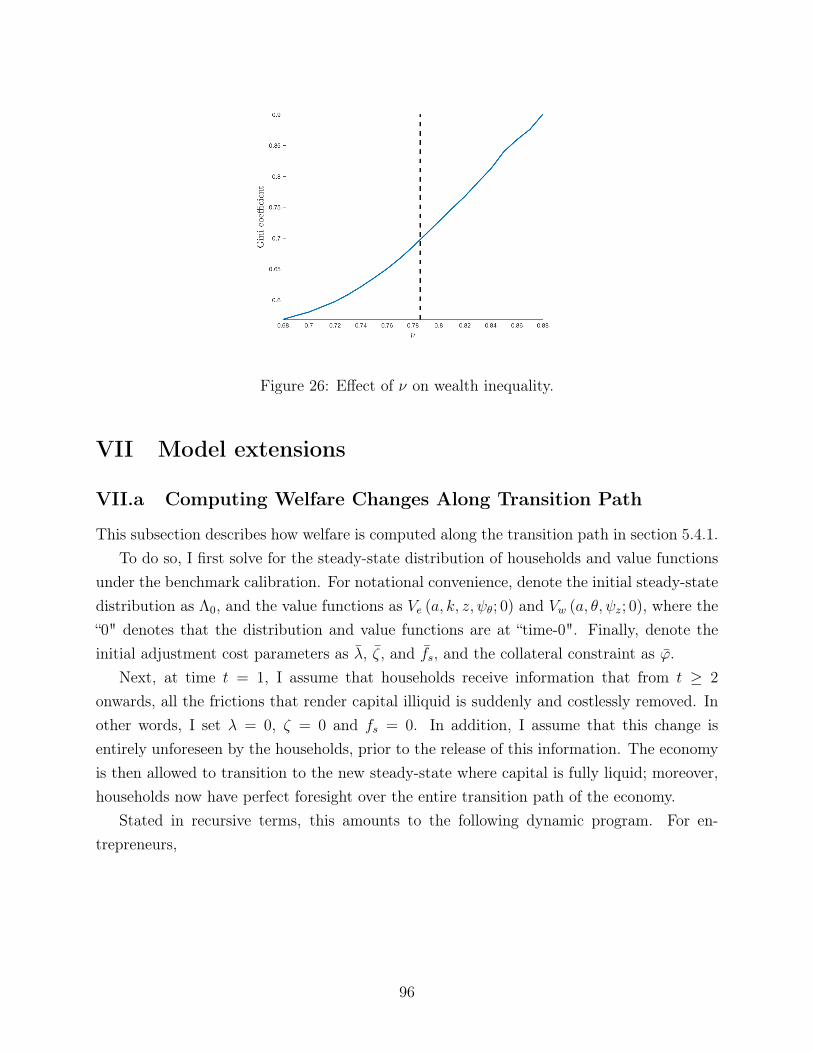
Figure 26: Effect of ν on wealth inequality.

VII Model extensions

VII.a Computing Welfare Changes Along Transition Path

This subsection describes how welfare is computed along the transition path in section 5.4.1.To do so, I first solve for the steady-state distribution of households and value functions

under the benchmark calibration. For notational convenience, denote the initial steady-statedistribution as Λ0, and the value functions as Ve (a, k, z, ψθ; 0) and Vw (a, θ, ψz; 0), where the“0" denotes that the distribution and value functions are at “time-0". Finally, denote theinitial adjustment cost parameters as λ, ζ, and fs, and the collateral constraint as ϕ.

Next, at time t = 1, I assume that households receive information that from t ≥ 2

onwards, all the frictions that render capital illiquid is suddenly and costlessly removed. Inother words, I set λ = 0, ζ = 0 and fs = 0. In addition, I assume that this change isentirely unforeseen by the households, prior to the release of this information. The economyis then allowed to transition to the new steady-state where capital is fully liquid; moreover,households now have perfect foresight over the entire transition path of the economy.

Stated in recursive terms, this amounts to the following dynamic program. For en-trepreneurs,

96

Ve(ψθ, z, k, b; t

)= max

h′,k′,b′,lU (c)

+ (1− h′)× β∫ψ′θ

∫z′Ve

(ψθ′, z′, k′, b′; t+ 1

)dPz′|zdFψθ

+ h′ × β∫ψ′z

∫θ′Vw

(ψz′, θ′, b′; t+ 1

)dPθ′|ψθdFψz

s.t.

π ≡ zf(k, ιl + l

)− wl +

(1 + r × 1{b≥0} + rd × 1{b<0}

)b− C (k′, k, h′, h; fst , λt, ζt, ϕt−1)

c = max {π, 0} − k′ − b′ ≥ 0

k′

> 0 if h′ = 0

= 0 if h′ = 1

h′ = 1 ( if π < 0)

b′ ≥ −ϕt (1− λt+1) (1− δ) k′ − b

c = c+ c

where

λt =

λ if t ≤ 1

0 if t ≥ 2

ζt =

ζ if t ≤ 1

0 if t ≥ 2

fst =

fs if t ≤ 1

0 if t ≥ 2

ϕt = ϕ

(1− λ

)(1− λt+1)

Note the explicit definition of the adjustment function C on the time-varying parameters,

97

as well as the adjustment of ϕ to fix the level of collateral constraint. For workers,

Vw (ψz, θ, b; t) = maxh′,k′,b′

U (c)

+ (1− h′)× β∫ψ′θ

∫z′Ve

(ψθ′, z′, k′, b′; t+ 1

)dPz′|ψzdFψθ

+ h′ × β∫ψ′z

∫θ′∈Θ

Vw

(ψz′, θ′, b′; t+ 1

)dPθ′|θdFψz

s.t.

c+ k′ + b′ = θwl +(1 + r × 1{b≥0} + rd × 1{b<0}

)b

k′

> 0 if h′ = 0

= 0 if h′ = 1

b′ ≥ −ϕt (1− λt+1) (1− δ) k′ − b

c = c+ c

The associated equilibrium conditions follows: A sequential competitive equilibrium ofthe model consist of the path of interest and wage rates {rt, wt)t≥0, value functions ofhouseholds and firms {Ve(·; t), Vw(·; t),Π(·; t)}t≥0, allocations {kt, bt, lt}t≥0 and distributionof agents Λt over the state space S such that,

1. Taking {rt, wt)t≥0 as given, the households’ and firms’ choices are optimal.

2. Markets clear, such that for every period t

(a) Bonds:∫btdΛt = Kc

t

(b) Labor:∫θhtdΛt =

∫ldΛ + Lct

3. The distribution Λt evolves as

Λt = Γt (Λt+1)

Where Γt is the one-period transition operator on the distribution at time t inducedby the policy functions of the households and firms.

For the partial equilibrium example, I fix interest rates and wages to the time 0 prices.To compute welfare, I then compare the time 0 value functions with the time 1 value

functions; that is to say, I compare the welfare of a household that lives in the benchmarkeconomy forever with that of an equivalent household who lives in the counter-factual econ-omy, taking into account the entire transitional dynamics associated with moving from the

98

initial economy to the new economy. The individual consumption equivalent variation, wel-fare changes for sub-populations, as well as the aggregate welfare changes are computed asdiscussed in the main text, using the time 0 distribution of households for aggregation.

VII.b Aggregate Shocks: Credit Tightening

To construct the dynamics in figure 19a, I assume that at time t = 0, ϕt = ϕ is held at itssteady state. At t = 1, the household’s collateral constraint suddenly tightens unexpectedly,such that ϕt < ϕ. However, at time t ≥ 2, the collateral constraint returns back to it’ssteady-state value. The households have full information of this reversion once the shockhits at t = 1. This, in a stylized fashion, replicates an exogenous credit tightening.

VII.c Aggregate Shocks: Increasing Illiquidity

To construct the dynamics in figure 19b, I assume that at time t = 0, λt = λ is held atits steady state. At t = 1, the price of used capital suddenly falls unexpectedly, such that1− λ < 1− λ. In order to avoid sudden default, I assume that λ1 stays at it’s steady-statevalue, but λ2 falls40. At t ≥ 3, the value of capital reverts back to it’s steady-state. Along thesame time path, the collateral constraint also adjusts such that the net collateral constraintis held fixed, as in section VII.a.This entire path is fully known to the household on e theshock hits at t = 1.

40Note that this does not mean that the shock is expected. Rather, one can consider this as similar to a“news shock".

99