Entrepreneurial Finance, Home Equity, andMonetary Policy∗

Paul JacksonUniversity of California, Irvine

Florian MadisonClaremont McKenna College

January 10, 2020

Abstract

We model entrepreneurial �nance using a combination of �at money, creditcards, traditional bank loans, and home equity loans. The banking sector is over-the-counter, where bargaining determines the pass-through from the nominalinterest rate to the bank lending rate, characterizing the transmission channelof monetary policy. The strength of this channel depends on the combinationof nominal and real assets used to �nance investments, and declines in theextent to which housing is accepted as collateral. A calibration to the U.S.economy complements the theoretical results and provides novel insights onentrepreneurial �nance between 2000 and 2016.

JEL Classi�cation: E22, E40, E52, G31, R31

Keywords: entrepreneurial �nance, money, housing, collateral, monetary policy

∗We are especially grateful to Guillaume Rocheteau and Aleksander Berensten for their extensive advice and support. Specialthanks also go to Randall Wright, Christopher Waller, David Andolfatto, Fernando Martin, Pedro Gomis-Porqueras, Ed Nosal,and Cyril Monnet for our fruitful discussions at the University of Bern and the FRB of St. Louis. Further we thank theparticipants of the 2018 Summer Workshop on Money, Banking, Payments and Finance at the FRB of St. Louis, the FifthMacro Marrakech Workshop at Université Cadi Ayyad, the Economic Theory Reading Group at the University of Basel, the UCIMacro Reading Group, and the participants at the 4th Macro Marrakesh Ph.D. workshop for their comments and thoughtfulquestions. This paper was previously titled �Corporate Finance, Home Equity, and Monetary Policy�. All errors are our own.Emails: pjackso1@uci.edu; �omadison@gmail.com.

1 Introduction

This paper provides a monetary search model subject to commitment and bargaining frictions

to study entrepreneurial �nance in the United States. Capital accumulation can be �nanced

internally using savings and credit card debt, and externally through traditional bank loans

and home equity loans, allowing for coexistence of money and credit. The banking sector

is over-the-counter, where bilateral bargaining determines the terms of trade, and thus the

pass-through from the nominal interest rate to the real lending rate, characterizing the

transmission channel of monetary policy.

It is well documented that apart from housing services, home equity is commonly used

as collateral to secure loans and lines of credit (HELs and HELOCs) when markets are

imperfect.1 While a fair share of these loans are used to �nance consumption (Greenspan

and Kennedy, 2007), they further �nd high demand among entrepreneurs facing capital

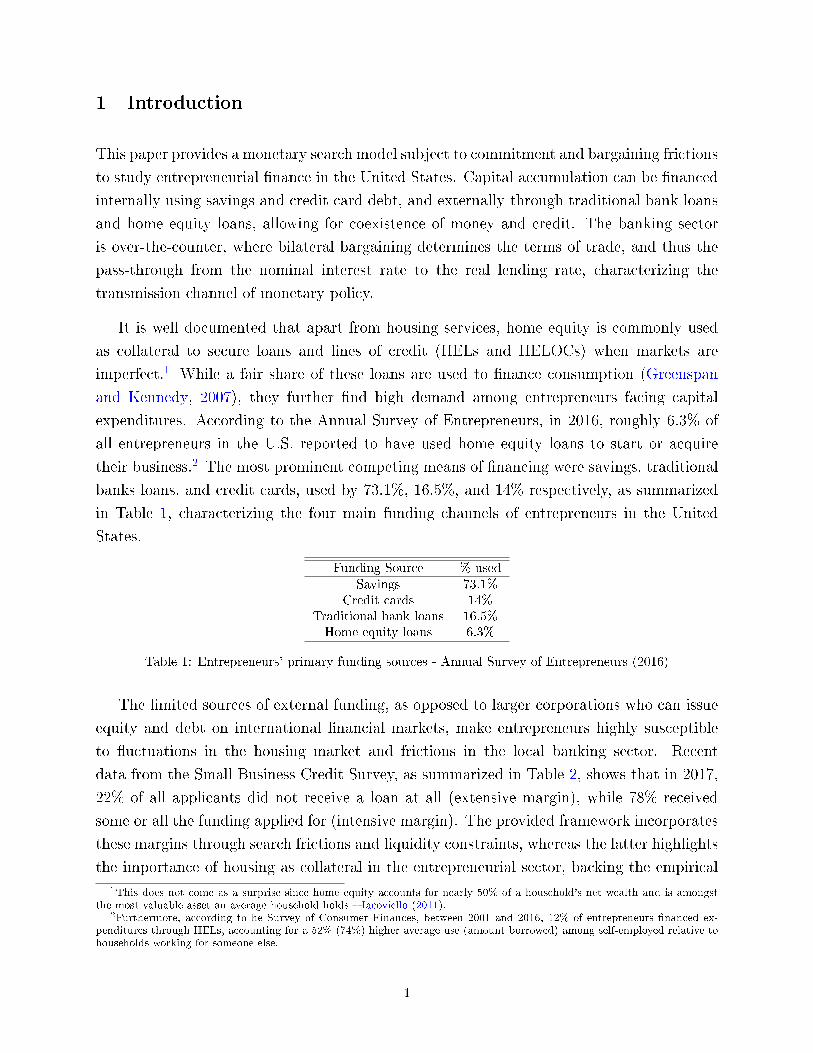
expenditures. According to the Annual Survey of Entrepreneurs, in 2016, roughly 6.3% of

all entrepreneurs in the U.S. reported to have used home equity loans to start or acquire

their business.2 The most prominent competing means of �nancing were savings, traditional

banks loans, and credit cards, used by 73.1%, 16.5%, and 14% respectively, as summarized

in Table 1, characterizing the four main funding channels of entrepreneurs in the United

States.

Funding Source %-used

Savings 73.1%Credit cards 14%

Traditional bank loans 16.5%Home equity loans 6.3%

Table 1: Entrepreneurs' primary funding sources - Annual Survey of Entrepreneurs (2016)

The limited sources of external funding, as opposed to larger corporations who can issue

equity and debt on international �nancial markets, make entrepreneurs highly susceptible

to �uctuations in the housing market and frictions in the local banking sector. Recent

data from the Small Business Credit Survey, as summarized in Table 2, shows that in 2017,

22% of all applicants did not receive a loan at all (extensive margin), while 78% received

some or all the funding applied for (intensive margin). The provided framework incorporates

these margins through search frictions and liquidity constraints, whereas the latter highlights

the importance of housing as collateral in the entrepreneurial sector, backing the empirical

1This does not come as a surprise since home equity accounts for nearly 50% of a household's net wealth and is amongstthe most valuable asset an average household holds � Iacoviello (2011).

2Furthermore, according to he Survey of Consumer Finances, between 2001 and 2016, 12% of entrepreneurs �nanced ex-penditures through HELs, accounting for a 52% (74%) higher average use (amount borrowed) among self-employed relative tohouseholds working for someone else.

1

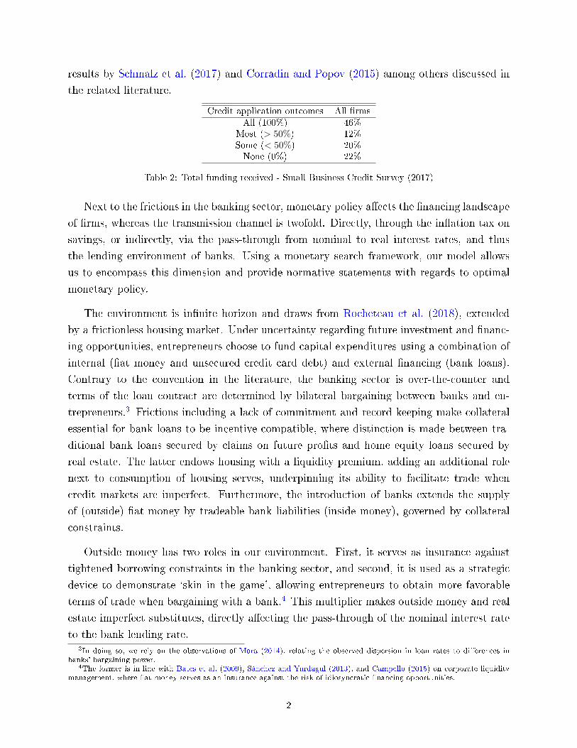
results by Schmalz et al. (2017) and Corradin and Popov (2015) among others discussed in

the related literature.

Credit application outcomes All �rms

All (100%) 46%Most (> 50%) 12%Some (< 50%) 20%None (0%) 22%

Table 2: Total funding received - Small Business Credit Survey (2017)

Next to the frictions in the banking sector, monetary policy a�ects the �nancing landscape

of �rms, whereas the transmission channel is twofold. Directly, through the in�ation tax on

savings, or indirectly, via the pass-through from nominal to real interest rates, and thus

the lending environment of banks. Using a monetary search framework, our model allows

us to encompass this dimension and provide normative statements with regards to optimal

monetary policy.

The environment is in�nite horizon and draws from Rocheteau et al. (2018), extended

by a frictionless housing market. Under uncertainty regarding future investment and �nanc-

ing opportunities, entrepreneurs choose to fund capital expenditures using a combination of

internal (�at money and unsecured credit card debt) and external �nancing (bank loans).

Contrary to the convention in the literature, the banking sector is over-the-counter and

terms of the loan contract are determined by bilateral bargaining between banks and en-

trepreneurs.3 Frictions including a lack of commitment and record keeping make collateral

essential for bank loans to be incentive compatible, where distinction is made between tra-

ditional bank loans secured by claims on future pro�ts and home equity loans secured by

real estate. The latter endows housing with a liquidity premium, adding an additional role

next to consumption of housing serves, underpinning its ability to facilitate trade when

credit markets are imperfect. Furthermore, the introduction of banks extends the supply

of (outside) �at money by tradeable bank liabilities (inside money), governed by collateral

constraints.

Outside money has two roles in our environment. First, it serves as insurance against

tightened borrowing constraints in the banking sector, and second, it is used as a strategic

device to demonstrate `skin in the game', allowing entrepreneurs to obtain more favorable

terms of trade when bargaining with a bank.4 This multiplier makes outside money and real

estate imperfect substitutes, directly a�ecting the pass-through of the nominal interest rate

to the bank lending rate.3In doing so, we rely on the observations of Mora (2014), relating the observed dispersion in loan rates to di�erences in

banks' bargaining power.4The former is in line with Bates et al. (2009), Sánchez and Yurdagul (2013), and Campello (2015) on corporate liquidity

management, where �at money serves as an insurance against the risk of idiosyncratic �nancing opportunities.

2

Relying on said pass-through and the two roles of outside money, the established model

provides novel insights on the transmission of monetary policy. The results show that the

magnitude of the real e�ects following a change in the nominal interest rate depends on

the composition of internal and external �nancing used, and hence the size of the haircuts

applied on the provided collateral. If housing is su�ciently pledgeable, the demand for �at

money is low, weakening the transmission channel of monetary policy. If, however, housing

is barely accepted as collateral and capital is primarily �nanced through internal �nancing

and traditional bank loans, the transmission channel is strong. The sensitivity of the pass-

through underpins the importance of the individual �nancing channels and highlights the

close relationship between the entrepreneurial sector, the housing market, and monetary

policy.

Given the environment, however, tractability of the analytical results is limited. Thus,

to complement the theoretical results, we calibrate the model to the U.S. economy for 2000-

2016. In doing so, we focus on the semi-elasticity of aggregate entrepreneurial investment in

response to a change in the nominal interest rate, capturing the strength of the transmission

of monetary policy. Varying the pledgeability of housing allows to account for �uctuations

in the housing market and consequential changes in the composition of internal and external

�nance. The calibrated results con�rm the aforementioned theoretical outcomes. For exam-

ple, at a nominal interest rate of 0.05 (as seen in 2007), if housing is denied as collateral,

a one percent increase in the nominal interest rate decreases entrepreneurial investment by

7.1%. The larger the share of investments �nanced by �at money, i.e., the lower the nominal

interest rate, the stronger the real e�ects of a change in monetary policy.

1.1 Related Literature

This paper is deeply founded in the literature on monetary search-theory and markets with

frictions, as surveyed in Rocheteau and Nosal (2017) and Lagos et al. (2017). The �rst

to apply the theoretical toolkit of this literature to study corporate �nance and monetary

policy, and the paper most closely related to ours, were Rocheteau et al. (2018). We build

on this framework by tailoring the environment to the entrepreneurial sector in the United

States, i.e, introducing credit card debt and a housing market, where private real estate

has two roles: consumption and saving. The latter allows entrepreneurs the use of home-

equity to secure bank loans, capturing the relationship between the housing market, the the

pass through from nominal to real rates, and the transmission channel to entrepreneurial

investment.5

5Another extension to study how heterogeneity of �nancial frictions and monopolistic competition in�uences this the trans-mission channel was provided by Silva (2017).

3

Since the Great Recession, a vast literature on the use of home equity to secure bilateral

credit transactions emerged, whereas distinction is made between consumption and invest-

ment loans. The former are studied by He et al. (2015), incorporating HELs into a Lagos and

Wright (2005) environment. The endogenously arising liquidity premium on housing gener-

ates dynamics in the value of real estate, explaining parts of the housing boom experienced

in the early 2000s.6 Using similar toolkits, Branch et al. (2016) provide an application to

unemployment by endogenizing the construction sector. Their results show that �nancial in-

novations that raise the acceptability of homes as collateral increase house prices and reduce

unemployment. Among the �rst to abstain from consumption loans were Liu et al. (2013),

introducing land as collateral in �rms' credit constraints using a DSGE model, showing how

co-movements of land prices and business investments propagate macroeconomic �uctua-

tions. While the provided results apply for �rms of all sizes, a more detailed application

to entrepreneurs is provided by Decker (2015). Within a heterogeneous agent DSGE model

with housing and entrepreneurship, his results show that while recessions accompanied by

a housing crash can explain the decline in entrepreneurial activity experienced in the early

2000s, a broader �nancial crisis would have no such e�ects. To further explain the recent

synchronization of house prices and entrepreneurial activity, Lim (2018) develops an occu-

pational choice model incorporating home equity loans. His results are in line with Decker

(2015) and the paper at hand, showing that a rise in house prices increases entrepreneurial

investment. However, a role for monetary policy remains absent. Our paper combines these

components, allowing for an analysis of entrepreneurial �nance, home equity, and monetary

policy.

We also draw on empirical work studying the importance of housing as collateral in

entrepreneurial �nance. Schmalz et al. (2017) found that higher values of collateral increased

the likelihood of becoming an entrepreneur and that those with higher values of collateral

took on more debt, started larger �rms, and were more likely to remain in the long run.

Corradin and Popov (2015) in turn focus on real estate prices in the U.S. and found that

a 10% increase in home equity increased the probability of becoming an entrepreneur by

7%. Adelino et al. (2015) estimated that the collateral lending channel could explain 15-25%

of employment variation in the U.S. between 2002-2012, showing the value of housing as

collateral is directly tied to the formation of new businesses. Black et al. (1996) used data

from the UK and found that a 10% increase in the value of home equity increased VAT

registrations by nearly 5%, suggesting that an increase in the value of housing led to more

small business formation. Harding and Rosenthal (2017) estimated that a 20% increase in real

home value over two years increased entry into self-employment by 15 percentage points and

6Complementary results are provided by Justiniano et al. (2015) and Garriga et al. (2018), studying the relationship betweenthe liquidity of real estate and house prices in the United States.

4

that self-employed homeowners are more likely to use home equity lines of credit. Abstaining

from the value of housing but focusing on its pledgeability, Jensen et al. (2014) found that

a reform in Denmark which increased the availability of home equity loans increased entry

into entrepreneurship.

The rest of this paper is organized as follows. Section 2 introduces the environment.

Section 3 solves the dynamic programming problem of the model, laying the foundation for

the bargaining game in Section 4 and optimal portfolio choice in Section 5. Monetary policy

is discussed in Section 6, followed by a calibration in Section 7. Last but not least, Section

8 concludes.

2 Environment

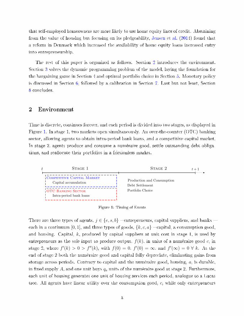
Time is discrete, continues forever, and each period is divided into two stages, as displayed in

Figure 1. In stage 1, two markets open simultaneously. An over-the-counter (OTC) banking

sector, allowing agents to obtain intra-period bank loans, and a competitive capital market.

In stage 2, agents produce and consume a numéraire good, settle outstanding debt obliga-

tions, and reallocate their portfolios in a frictionless market.

Stage 1 Stage 2

Competitive Capital Market

OTC Banking Sector

t t+ 1

Capital accumulation

Intra-period bank loans

Production and Consumption

Debt Settlement

Portfolio Choice

Figure 1: Timing of Events

There are three types of agents, j ∈ {e, s, b} � entrepreneurs, capital suppliers, and banks �

each in a continuum [0, 1], and three types of goods, {k, c, a} � capital, a consumption good,

and housing. Capital, k, produced by capital suppliers at unit cost in stage 1, is used by

entrepreneurs as the sole input to produce output, f(k), in units of a numéraire good c, in

stage 2, where f ′(k) > 0 > f ′′(k), with f(0) = 0, f ′(0) = ∞, and f ′(∞) = 0 ∀ k. At the

end of stage 2 both the numéraire good and capital fully depreciate, eliminating gains from

storage across periods. Contrary to capital and the numéraire good, housing, a, is durable,

in �xed supply A, and one unit buys qa units of the numéraire good at stage 2. Furthermore,

each unit of housing generates one unit of housing services each period, analogue to a Lucas

tree. All agents have linear utility over the consumption good, c, while only entrepreneurs

5

value housing services, ϑ(a), where ϑ′(a) > 0 > ϑ′′(a), ϑ(0) = 0, ϑ′(0) =∞, and ϑ′(∞) = 0 ∀a. The discount factor across periods is β = (1 + r)−1 and r > 0 the rate of time preference,

characterizing the entrepreneur's lifetime utility:

E∞∑t=0

βt[ct + ϑ(at)]. (1)

There is no record keeping of transactions in the competitive capital market and en-

trepreneurs have limited ability to commit to future actions. Hence, given the timing of

events (supplier providing k in stage 1 and entrepreneur producing c in stage 2) and the

non-durability of capital and the numéraire good, media of exchange � money and/or credit

� are essential for trade to occur.

We allow for internal and external �nancing. Internal �nancing consists of �at money

(savings), m, and intra-period credit card debt, b ∈ [0, b̄], up to an exogenous debt limit

b̄. There is a central bank managing the supply of �at money in the economy according to

M ′ = (1+τ)M , whereM denotes the stock of �at money in the current period,M ′ the stock

in the next period, and expansion/contraction is conducted through lump-sum transfers,

T = τMt. One unit of money can buy qm units of the numéraire good in stage 2. Since we

focus on symmetric and stationary monetary equilibria, it holds that M ′/M = qm/q′m = γ

with γ being the exogenous gross growth rate of the �at money supply. External �nancing, on

the other hand, can be obtained through banks via intra-period loans, consisting of perfectly

divisible and recognizable one-period liabilities (inside money), i.e., banks can commit.7

Given the lack of record-keeping and an entrepreneur's limited ability to commit to future

actions, bilateral loans need to be collateralized to be incentive compatible. We consider

(partial)-pledgeability of housing (HELs), ρqaa, and future output (traditional bank loans),

χf(k), with ρ ≤ 1 and χ ≤ 1.8 Hence, expansion and contraction of inside money is bounded

by collateral constraints. Settlement of loan obligations, l, takes place in stage 2, where given

the banks' ability to commit to future actions, redemption of collateral is guaranteed. In

case of default on the part of the entrepreneur, the bank keeps the collateral.

Two idiosyncratic uncertainties determine the composition of internal and external �-

nancing: the availability of production/investment opportunities (as in Kiyotaki and Moore

(1997)) and the availability of �nancing opportunities (as in Wasmer and Weil (2004)). With

probability λ ∈ [0, 1], an entrepreneur encounters an investment opportunity at the begin-

7Said liabilities are perfectly recognizable within a period, but can be counterfeited thereafter, which precludes them fromcirculating across periods.

8We assume that housing and future output are pledgeable only to banks, as banks are the only agents who have thetechnology to verify home-ownership and recover investments. Thus, there is no trade credit between capital suppliers andentrepreneurs.

6

ning of stage 1, guaranteeing access to the production technology f(k) in stage 2. Once

encountered, with probability α ∈ [0, 1], he meets a banker in the OTC banking sector who

is willing to provide a loan. Assuming independence, with probability λα an investment op-

portunity is �nanced internally and externally, while with probability λ(1−α), an investment

opportunity is solely �nanced internally.

At the end of stage 2, entrepreneurs consume the produced numéraire good, c, housing

services, ϑ(a), settle outstanding credit obligations, l ∈ R+ and b ∈ R+, and adjust their

portfolio consisting of �at money, and housing, m and a.

3 Model

An entrepreneur enters stage 2 with k units of capital and �nancial wealth, ω, denoted in the

numéraire consisting of real money balances qmm and housing qaa, minus bank and credit

card liabilities, l and b, to solve:

W e(k, ω) = maxc,m′,a′

c+ ϑ(a) + βV e(m′, a′) (2)

s.t. c = f(k) + T + ω − qmm′ − qaa′, (3)

where βV e(m′, a′) is the continuation value in stage 1 of the next period. Plugging (3) into

(2), yields:

W e(k, ω) = f(k) + ϑ(a) + ω + T + maxm′,a′{−qmm′ − qaa′ + V e(m′, a′)}. (4)

Hence, since W e(k, ω) is linear in current wealth, an entrepreneur's choice of �at money and

housing for the subsequent stage 1, (m′, a′), is independent of current balances (k, ω). The

entrepreneur's value function in stage 1 is:

V e(m, a) = (1− λ)W e(0, ω) + λ[(1− α)W e(kI , ω) + αW e(kE, ω)], (5)

where capital accumulation is conditional on α and λ with kI representing only internally

�nanced capital and kE internally and externally �nanced capital. Plugging (5) into (4) and

updating reduces the portfolio choice in stage 2 to:

maxm′,a′−[qm/β − q′m]m′ − [qa/β − q′a]a′ + ϑ(a′) + λ[(1− α)∆e

I(m′, b′) + α∆e

E(m′, a′, b′)], (6)

with ∆eI(m, b) and ∆e

E(m, a, b) denoting the entrepreneur's surpluses using internal and ex-

ternal �nancing, respectively. Following perfect competition in the capital market, ∆eI(m, b)

7

is de�ned as ∆eI(m, b) = f(kI) − kI with kI = min{qmm + b̄, k∗}, where k∗ solves k∗ ∈

arg maxk[f(k)− k] > 0, analogue to the planner's problem. It represents the entrepreneur's

outside option �nancing investments with savings and credit card debt only, playing a cru-

cial role when determining ∆eE(m, a, b) via bilateral bargaining between a bank and an en-

trepreneur in Section 4.9 Once determined, Section 5 characterizes the entrepreneur's optimal

portfolio choice in stage 2, paving the way to study optimal policy in Section 6.

Analogue to the entrepreneur, the value functions of a bank and a capital supplier in

stage 2 and 1 are:

W b,s(k, ω) = maxm′,a′

ω − qmm′ − qaa′ + βV b,s(m′, a′) (7)

and

V b(m, a) = (1− λ)W b(0, ω) + λ[(1− α)W b(0, ω) + αW b(0, ω + φ)] (8)

V s(m, a) = maxk{−k +W s(0, ω + qkk)}, (9)

where φ denotes the bank's intra-period loan pro�ts determined via bilateral bargaining in

Section 4 and qkk the capital supplier's proceeds from capital sales in stage 1. The linearity

of W s implies qk = 1, and hence W s = V s. Plugging either (8) into (7) or (9) into (7) yields:

maxm′,a′−[qm/β − q′m]m′ − [qa/β − q′a]a′, (10)

for both banks and capital suppliers. Thus, if the rate of return of money and housing is

non-positive, i.e., if qm/β ≥ q′m and qa/β ≥ q′a, neither capital suppliers nor banks have an

incentive to hold positive positions, and hence (ms, as) = (mb, ab) = (0, 0).

4 Bargaining

The terms of the loan contract, (kE, φ, d, y, b), are determined via proportional bargaining,

where kE denotes the total amount of capital �nanced, φ the bank's service fee, y ∈ [0, a] the

amount of housing used as collateral, d ∈ [0,m] the monetary downpayment, and b ∈ [0, b]

credit card debt. Let S = Se + Sb be the total surplus to be bargained over:

Se ≡ W e(kE, ω)−W e(kI , ω) = f(kE)− kE − φ−∆eI(m, b), (11)

Sb ≡ W b(0, ω + φ)−W b(0, ω) = φ, (12)

9Savings and credit card debt are used as monetary downpayment to represent 'skin in the game' when negotiating the termsof the loan contract with a bank.

8

characterizing the following bargaining problem:

(kE, φ, d, y, b) ∈ arg max f(kE)− kE − φ−∆eI(m, b), (13)

s.t. θ[f(kE)− kE − φ−∆eI(m, b)] ≥ (1− θ)φ, (14)

s.t. l ≡ kE − qmd− b+ φ ≤ χf(kE) + ρqay, (15)

where θ ∈ [0, 1] represents the bank's bargaining power, and (14) governs how the total

surplus is split proportionally between the bank and the entrepreneur. Equation (15) is the

entrepreneur's liquidity constraint and determines the size of the future loan obligation, l,

where ρqay is the collateral value of housing and χf(kE) the collateral value of future output.

Debt limits are imposed exogenously following Kiyotaki and Moore (1997) with χ (ρ) being

the fraction of future output (housing) pledgeable to the bank.10 It follows immediately that

the size of the loan obligation, l, decreases with the monetary downpayment, i.e., the amount

of capital �nanced internally using savings and credit card debt, qmd and b.

De�nition A. An equilibrium of the bargaining game between an entrepreneur and a bank is

a pair of strategies, (kE, φ, d, y, b), such that the terms of trade, (kE, φ, d, y, b), are a solution

to the bargaining problem (13)-(15).

If the entrepreneur's liquidity constraint, (15), does not bind, the entrepreneur may

achieve the socially-e�cient level of investment, kE = k∗. Using (14) and solving for φ gives:

φ = θ[f(k∗)− k∗ −∆eI(m, b)], (16)

denoting the bank's fraction of the total match surplus. Comparative statics show that

∂φ/∂∆eI(m, b) < 0, so the fee collected by the bank is decreasing in the value of the en-

trepreneur's outside option. Thus, apart from being an insurance against not receiving a

bank loan, �at money incorporates a strategic role in the bargaining game, reducing the

bank's surplus. In the limiting case with χ = 0 and ρ = 0 (no bank loan), kE = kI = k∗ if

qmm + b̄ ≥ k∗. If, however, qmm + b̄ < k∗, then kI < kE ≤ k∗, where kE ≤ k∗ holds with

equality if either output or housing is su�ciently pledgeable. Plugging (16) into (15), we

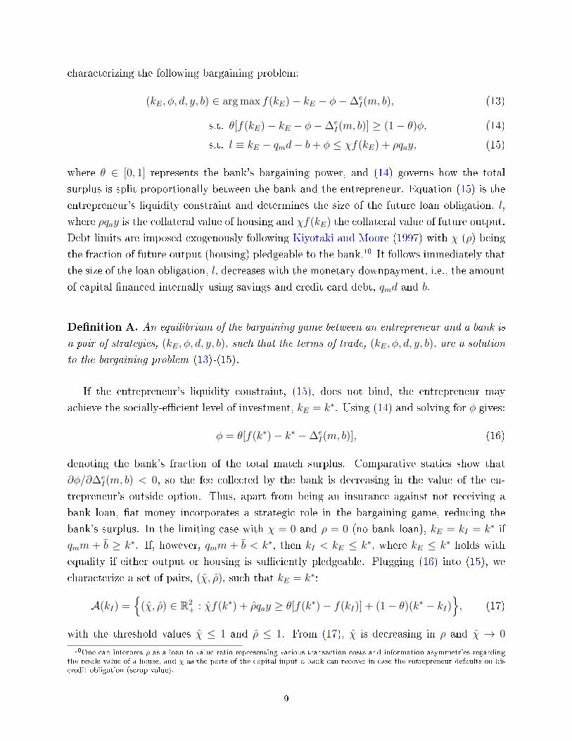
characterize a set of pairs, (χ̂, ρ̂), such that kE = k∗:

A(kI) ={

(χ̂, ρ̂) ∈ R2+ : χ̂f(k∗) + ρ̂qay ≥ θ[f(k∗)− f(kI)] + (1− θ)(k∗ − kI)

}, (17)

with the threshold values χ̂ ≤ 1 and ρ̂ ≤ 1. From (17), χ̂ is decreasing in ρ and χ̂ → 0

10One can interpret ρ as a loan-to-value ratio representing various transaction costs and information asymmetries regardingthe resale value of a house, and χ as the parts of the capital input a bank can recover in case the entrepreneur defaults on hiscredit obligation (scrap value).

9

ρ

χ1

1

ρ∗

χ∗

ρ′∗

χ′∗

A(kI)

kI ↑

Figure 2: Set A(kI) in an Unconstrained Equilibrium

as ρ → ρ∗, where ρ∗ allows entrepreneurs to accumulate k∗ when χ = 0 (analogue for χ∗).

The same, but vice versa, holds for ρ̂. Furthermore, with an increase in kI , A(kI) converges

towards the origin, since there are more combinations of χ and ρ that allow for kE = k∗.

Figure 2 illustrates.

Consider now the case where the entrepreneur's liquidity constraint, (15), is binding.

Solving (14) for φ and substituting into (15) with d = m, y = a, and b = b gives:

(1− θ)kE + θ[f(kE)−∆em(m)] = χf(kE) + ρqaa+ qmm+ b, (18)

which determines kE. The corresponding comparative statics show that ∂kE/∂θ < 0,

∂kE/∂kI > 0, ∂kE/∂qaa > 0, ∂kE/∂ρ > 0, and ∂kE/∂χ > 0. Lemma A summarizes.

Lemma A. There exists a unique solution to (13) with kI ∈ min{qmm + b̄, k∗}. If χ < χ∗

and ρ < ρ∗, there exists an m∗ such that k∗ > qmm∗+ b̄ and the following is true: If m ≥ m∗,

the solution to (13) is:

kE = k∗, (19)

φ = θ[f(k∗)− k∗ −∆eI(m, b)]. (20)

If m < m∗, however, then (φ, kE) solves:

φ = θ[f(kE)− kE −∆eI(m, b)], (21)

θ[f(kE)− kE −∆eI(m, b)] = χf(kE) + ρqaa− kE + kI , (22)

10

kI

rb

θ[f(k∗)−k∗]k∗

k∗

Figure 3: Bank Lending Rate

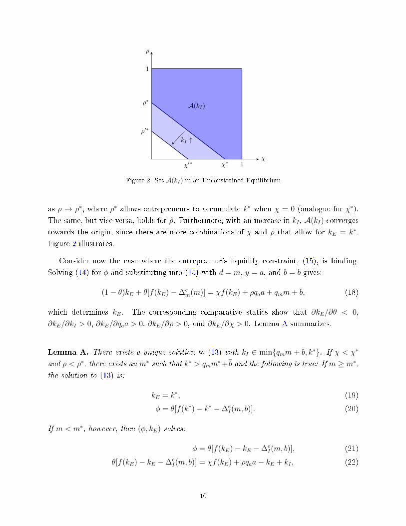
and kE ≥ kE, where χf′(kE) = 1. Proof in Appendix A.

It is important to note that in equilibrium ∂[kI + χf(kE) + ρqaa]/∂kI > 1, and thus by

carrying an additional unit of �at money along the period, entrepreneurs can increase their

accumulated capital by more than one unit. The intuition behind this result is straightfor-

ward. An additional unit of �at money does not only buy the entrepreneur more capital from

the supplier, but also signalizes a higher investment to the bank, enabling the entrepreneur

to credibly pledge more future output. Lemma B revisits this result and determines its im-

plications for the bank lending rate.

Lemma B. The bank lending rate, rb, de�ned as the ratio of the fee, φ, to the loan size,

kE − kI , is given by:

rb =φ

kE − kI=

θ[f(k∗)− k∗ −∆e

I(m, b)]

k∗ − kIif m ≥ m∗,

θ[f(kE)− kE −∆eI(m, b)]

kE − kIif m < m∗,

(23)

where, given qm, χ and ρ, m∗ is the minimal amount of �at money the entrepreneur needs

to attain k∗ through bank credit. Proof in Appendix B.

From Lemma B and Figure 3, the bank lending rate is decreasing in kI , as the entrepreneur

faces a more valuable outside option, ∆eI(m, b). Hence, the more real money balances an

entrepreneur is able to bring into the stage 1, i.e., the more capital is �nanced internally,

the lower the real lending rate, ∂rb/∂kI < 0. This pass-through is revisited in more detail

in Sections 6 and 7.

11

5 Portfolio Choice

To determine the entrepreneur's optimal portfolio choice in stage 2, we revisit (6):

maxm′,a′−[qm/β − q′m]m′ − [qa/β − q′a]a′ + ϑ(a′) + λ[(1− α)∆e

I(m′, b′) + α∆e

E(m′, a′, b′)], (24)

with

∆eI(m, b) =

{f(k∗)− k∗ if qmm+ b̄ ≥ k∗

f(kI)− kI if qmm+ b̄ < k∗,(25)

∆eE(m, a, b) =

{(1− θ)

[f(k∗)− k∗

]+ θ∆e

I(m, b) if m ≥ m∗

(1− χ)f(kE)− ρqaa− kI if m < m∗,(26)

where the terms of trade [kI(m, b̄), kE(m, a, b̄), φ(m, a, b̄), d(m, a, b̄), y(m, a, b̄), b(m, a, b̄)] are

a function of the entrepreneur's credit card limit and aggregate money and housing. The

�rst term, − [qm/β − q′m]m′, represents the opportunity costs of carrying �at money across

the period, while −[qa/β − q′a]a′ is the cost of holding real estate.

De�nition B. An equilibrium in the stage 2 is a list of portfolios, terms of trade in stage

1, and aggregate balances, {[m(·), a(·)], [kI(·), kE(·), φ(·), d(·), y(·), b(·)],M,A}, such that:

(i) [m(·), a(·)] is a solution to (24);

(ii) kI = min{qmm+ b̄, k∗};

(iii) [kE(·), φ(·), d(·), y(·), b(·)] is a solution to (13);

(iv) M ′ = (1 + τ)M is the law of motion of the �at money stock;

(v) A is the total supply of housing in the economy; and

(vi) Market clearing conditions,∫ 1

0a(j)dj = A and

∫ 1

0m(j)dj = M , hold.

Lemma C. There exists a unique solution to (24):

qm = βq′m[1 + Lm], (27)

qa = β[q′a(1 + La) + ϑ′(a)], (28)

12

with (Lm,La) = (0, 0) for kI = k∗, and:

Lm =

λ[1− α(1− θ)][f ′(kI)− 1] for kE ≥ k∗,

λα

[(1− χ)f ′(kE)[1 + θ(f ′(kI)− 1)]

(1− θ)− (χ− θ)f ′(kE)− 1

]+ λ(1− α) [f ′(kI)− 1] for kE < k∗,

La =

0 for kE ≥ k∗,

λαρ

[(1− χ)f ′(kE)

1− θ − (χ− θ)f ′(kE)− 1

]for kE < k∗,

(29)

where Lm and La correspond to the liquidity premia of money and housing, respectively.

Proof in Appendix C.

Consider the three cases from the bargaining game in Section 4: kI ≥ k∗, kE ≥ k∗,

and kE < k∗. If money is costless to hold, i.e. Lm = 0, an entrepreneur obtains enough

�at money to purchase kI = k∗. As a consequence, housing is priced at its fundamental

value with La = 0. If Lm > 0, however, money is costly to hold and kI < k∗. As a

consequence, there is demand for external �nance. Two cases need to be considered: If the

entrepreneur's liquidity constraint, (15), is non-binding, then kE ≥ k∗. Nonetheless, money

incorporates a positive liquidity premium, Lm > 0, since an additional unit would increase

the entrepreneur's outside option, ∆eI(m, b), and hence decrease the cost of borrowing form

a bank. Housing, however, still trades at the fundamental value, i.e., La = 0, since the

entrepreneur is not constrained in the amount of collateral carried into stage 1. If (15) is

binding, however, then kE < k∗. As a consequence, La > 0 since an additional unit of

housing would relax (15). The costlier �at money, the larger the premium.

6 Monetary Policy and the Transmission Mechanism

Having determined the bargaining game and the general equilibrium results of the model,

this section characterizes optimal monetary policy. We start by characterizing the nomi-

nal interest rate, followed by an analysis of the pass-through to understand how changes in

monetary policy a�ect the terms of trade in the banking sector. Last but not least, we then

analyze the transmission of monetary policy to aggregate investment and lending.

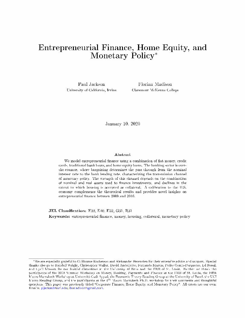
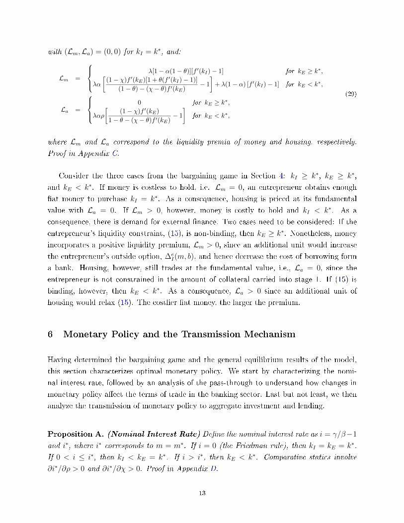
Proposition A. (Nominal Interest Rate) De�ne the nominal interest rate as i = γ/β−1

and i∗, where i∗ corresponds to m = m∗. If i = 0 (the Friedman rule), then kI = kE = k∗.

If 0 < i ≤ i∗, then kI < kE = k∗. If i > i∗, then kE < k∗. Comparative statics involve

∂i∗/∂ρ > 0 and ∂i∗/∂χ > 0. Proof in Appendix D.

13

i

qmm∗

k∗

qmm

kE

l(i)

kI

i∗ ii∗

qa

Figure 4: Money and Housing Demand

Proposition A characterizes optimal monetary policy using the general equilibrium results

in Section 5, as visually represented in Figure 4. Comparative statics show that an increase

in the pledgeability of housing or future output, ρ and χ, increases i∗.

In order to study the pass-through of the nominal interest rate, i, to the bank lend-

ing rate, rb, we rely on �rst-order Taylor approximations. Distinction is made between an

unconstrained and a constrained equilibrium. In an unconstrained equilibrium, we use a

�rst-order approximation of the equilibrium for i close to 0, and hence kI close to k∗. We

take this approach for two reasons. First, if i ≈ 0, then kI < k∗, and thus bank credit is

essential. Second, it allows for closed form solutions. To analyze a constrained equilibrium

and maintain analytical tractability, we set θ = 0 and take a �rst-order approximation of an

equilibrium where i ≈ i∗ and thus kE ≈ k∗. While setting the bank's bargaining power to

zero implies rb = 0, we are still able to derive closed form approximations for kI and kE. A

more general analysis with θ > 0 is provided in the calibration in Section 7. With this in

mind, Proposition B summarizes.

Proposition B. (Pass-Through) For i ≈ 0, the pass-through of the nominal interest rate

to the bank lending rate is approximated by:

rb ≈ θi

2λ[1− α(1− θ)] . (30)

For i ≈ i∗, however, rb = 0 since θ = 0. Comparative statics involve ∂rb/∂λ < 0, ∂rb/∂θ > 0,

and ∂rb/∂α > 0. Proof in Appendix E.

For i ≈ 0, equation (30) identi�es a positive pass-through from the nominal interest rate

to the bank lending rate, ∂rb/∂i > 0, since entrepreneurs rely more on external �nance. For

14

i ≈ i∗, however, the pass-through cannot be characterized, since we set θ = 0 for analytical

tractability. Further comparative statics show that an increase in λ weakens the pass-through

from the nominal interest to the bank lending rate, while an increase in θ or α strengthens

the pass-through. Moreover, a change in ρ or χ has no e�ect on the pass through.

With this understanding, we proceed to analyze the transmission of monetary policy to

aggregate investment and lending, K ≡ λ[(1 − α)kI + αkE] and L ≡ λα(kE − kI). Let

k̄ = k∗ − χf(k∗)− ρaβϑ′(a)1−β and i∗ = λ(1− α)[f ′(k̄)− 1], where k̄ is de�ned as the minimum

kI an entrepreneur needs to obtain kE = k∗ after having pledged all of his private real estate

and claims on future output, and i∗ is the corresponding nominal interest rate. For i ≈ 0

and thus kE ≈ k∗, the transmission of the nominal interest rate to aggregate investment and

lending is approximated by:11

K ≈ λk∗ +(1− α)i

f ′′(k∗)[1− α(1− θ)] , (31)

L ≈ −αif ′′(k∗)[1− α(1− θ)] . (32)

For i− i∗ ≈ 0 and θ = 0, however,

kE − k∗ ≈kI − k̄1−O ≈ −

i− i∗D

, (33)

L ≈ λα

[k∗ − k̄ − O(i− i∗)

D

], (34)

where D > 0, and:

O = χ+

(βρ

1− β

)2[αλaϑ′(a)f ′′(k∗)

1− χ

]. (35)

Proposition C summarizes the transmission mechanism.

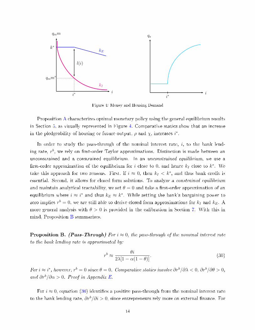
Proposition C. (Transmission Mechanism) For θ = 0, χ < χ∗, and ρ < ρ∗, transmis-

sion of monetary policy to aggregate investment and lending is characterized by the following

three regions:

A : i ≤ i∗ with ∂kI/∂i < ∂kE/∂i = 0, and ∂L/∂i > 0,

B : i > i∗ with ∂kI/∂i < ∂kE/∂i < 0, and ∂L/∂i > 0,

C : i > i∗ with ∂kE/∂i < ∂kI/∂i < 0, and ∂L/∂i < 0,

11Details to the derivation can be found in Appendix H.

15

ρ

χ

A

B

C

Figure 5: Transmission to aggregate investment and lending

as represented in Figure 5 and equations (31)-(35). Comparative statics show:

∂|∂kE/∂i|/∂ρ = 0 for i ≤ i∗,

∂|∂kE/∂i|/∂ρ < 0 for i > i∗.

Proof in Appendix F.

Proposition C analyzes the e�ect of a change in the nominal interest rate on aggregate

investment and lending, characterizing three distinct regions. In region A, i ≤ i∗, and thus

the entrepreneur's liquidity constraint, (15), does not bind. As a consequence, kI decreases

with an increase in i, while kE remains una�ected. From (32), aggregate lending is increasing

in i, as entrepreneurs rely more on external �nance. For i > i∗, however, an increase in i

decreases both internally and externally �nanced capital. Given (33) and (35), the strength

of this e�ect depends on the composition, i.e., the combination of savings, credit card debt,

traditional bank loans, and HELs used to purchase kE. The e�ect on aggregate lending,

i.e., ∂L/∂i, follows this outcome. Consider �rst region B, in which an entrepreneur relies

extensively on HELs. In this scenario, kI will decrease more than kE in response to an increase

in i, as entrepreneurs successfully hedge against in�ation by using their real asset (housing)

when bargaining with the bank. The increased demand for housing and the consequential

price appreciation increases L and weakens the transmission channel of monetary policy.

In contrast, in region C, an increase in the nominal interest rate, i, decreases kE more

than kI , implying a decrease in aggregate lending, L. Thus, whenever the pledgeability of

housing is limited, entrepreneurs are unable to alleviate the in�ation tax and as a result,

the appreciation in the house prices does not compensate for the reduction in real money

balances and the consequentially worse terms of trade when bargaining with a bank. Further,

comparative statics show that for region B and C, an increase in ρ weakens the transmission

16

mechanism, while in region A, a change in ρ has no e�ect on |∂kE/∂i|.

7 Calibrated Results

Having characterized the transmission channel analytically, we now complement the previous

results with a calibrated version of the model. The key di�erence to the previous Taylor

approximations is that we allow banks to have a positive bargaining power (θ > 0), enabling

an analysis of the pass-through in a constrained equilibrium.

The model is calibrated to U.S. data covering 2000-2016.12 We start by setting the

discount factor to β = 0.97. Our measure for the nominal interest rate is the 3-month

T-bill secondary market rate with an average of i = 0.0163. The probability to have a

bank loan approved, α, is 0.80 following the 2003 Survey of Small Business Finances. The

pledgeability of future output is calculated as the average ratio of liabilities to assets among

small businesses. From the Federal Reserve Flow of Funds Accounts, we calculate χ = 0.24.

The pledgeability of housing, ρ, is set equal to the average ratio of home equity loan limits

to the average sale price of U.S. homes between 2006 and 2016. Using data from the Federal

Reserve Bank of New York's Quarterly Report on Household Debt and Credit and the FRED

database, we �nd ρ = 0.18. We then choose b to match the average ratio of credit card limits

to home equity loan limits and �nd b = 0.3783.13 We estimate the probability of receiving

an investment opportunity, λ, by calculating the average percentage of entrepreneurs who

started their business within the last year. Using data from the Survey of Consumer Finances

(SCF) between 2001 and 2016, we estimate λ = 0.0628. To pin down θ, we follow Rocheteau

et al. (2018) in targeting the spread between the prime bank rate and the 3-month T-bill

rate of 3.25%, i.e. rb − i = 0.0325.14 Last but not least, we de�ne the functional forms

for the entrepreneur's production function, f(k) = νkη, and the utility of housing services,

ϑ(a) = a1/2, where ν = β/(1− β) is a scaling parameter.15

To study the transmission mechanism of monetary policy, we focus on the pass-through

rate, ∂rb/∂i, and the semi-elasticity of aggregate investment and aggregate lending, i.e., the

percentage change in response to a one percentage point increase in the nominal interest

rate, ∂log(K)/∂i, and ∂log(L)/∂i. By varying the pledgeability of housing, ρ, between 0

and 1, we account for changes in the composition of �nancing. We focus on these e�ects for

12See Appendix G for details on data sources and calculations.13Using data from the Federal Reserve Bank of New York's Quarterly Report on Household Debt and Credit we �nd the

average ratio of credit card limits to home equity loan limits, between 2003-2016, to be 0.13.14For 0 < i < i∗, rb is given by equation (23) for the case of m > m∗. We check that under the parameters in Table 3, an

entrepreneur's liquidity constraint does not bind for i < 0.0233.15Recall that the fundamental value of housing is qa = βϑ′(A)/1−β . Without scaling the production function, say if f(k) = kη ,

entrepreneurs would mechanically be able to obtain k∗ through bank loans (as f ′(k∗) = 1) for ρ > 0.

17

Parameter De�nition Value Target

β Discount factor 0.97 Annual frequencyi Nominal interest rate 0.0163 3-month T-bill rateα Probability of receiving bank credit 0.80 Loan acceptance rateλ Probability of receiving an investment opportunity 0.0628 Formation of new businessesθ Bank's bargaining power 0.162 Spreadχ Fraction of future output that is pledgeable 0.24 Asset-to-liability ratioρ Fraction of housing that is pledgeable 0.18 HE limit-to-home price ratio

b Maximum amount of unsecured credit 0.3783 Credit card limit-to-HE limit ratioη Capital share 1/3 Fixed

Table 3: Parameter values

i ∈ [0, 0.12], whereas the calibration determines i∗ = 0.0308.

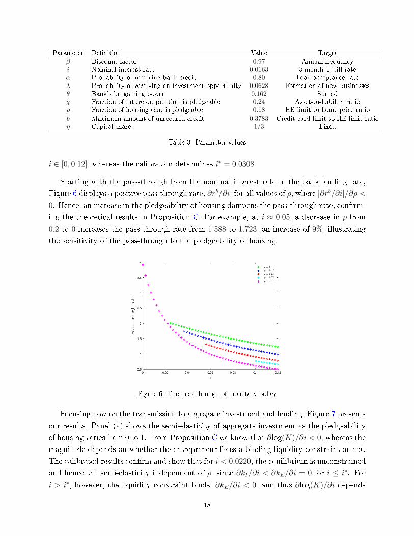
Starting with the pass-through from the nominal interest rate to the bank lending rate,

Figure 6 displays a positive pass-through rate, ∂rb/∂i, for all values of ρ, where |∂rb/∂i|/∂ρ <0. Hence, an increase in the pledgeability of housing dampens the pass-through rate, con�rm-

ing the theoretical results in Proposition C. For example, at i ≈ 0.05, a decrease in ρ from

0.2 to 0 increases the pass-through rate from 1.588 to 1.723, an increase of 9%, illustrating

the sensitivity of the pass-through to the pledgeability of housing.

Figure 6: The pass-through of monetary policy

Focusing now on the transmission to aggregate investment and lending, Figure 7 presents

our results. Panel (a) shows the semi-elasticity of aggregate investment as the pledgeability

of housing varies from 0 to 1. From Proposition C we know that ∂log(K)/∂i < 0, whereas the

magnitude depends on whether the entrepreneur faces a binding liquidity constraint or not.

The calibrated results con�rm and show that for i < 0.0220, the equilibrium is unconstrained

and hence the semi-elasticity independent of ρ, since ∂kI/∂i < ∂kE/∂i = 0 for i ≤ i∗. For

i > i∗, however, the liquidity constraint binds, ∂kE/∂i < 0, and thus ∂log(K)/∂i depends

18

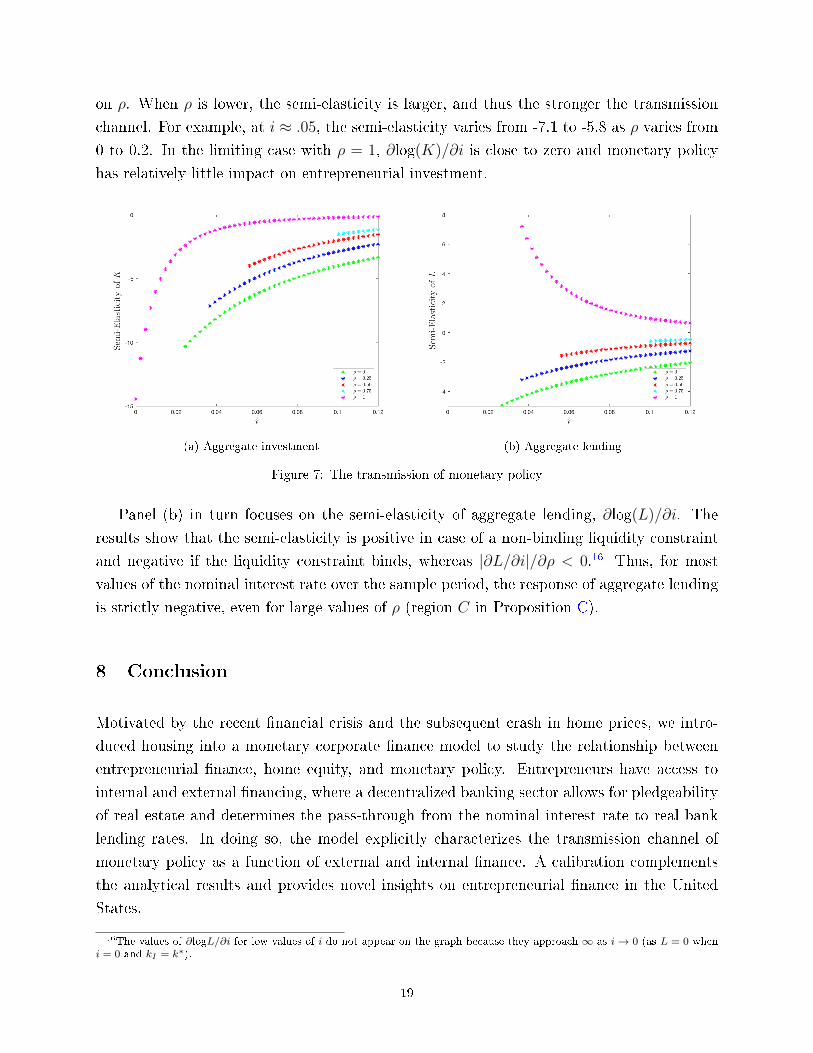
on ρ. When ρ is lower, the semi-elasticity is larger, and thus the stronger the transmission

channel. For example, at i ≈ .05, the semi-elasticity varies from -7.1 to -5.8 as ρ varies from

0 to 0.2. In the limiting case with ρ = 1, ∂log(K)/∂i is close to zero and monetary policy

has relatively little impact on entrepreneurial investment.

(a) Aggregate investment (b) Aggregate lending

Figure 7: The transmission of monetary policy

Panel (b) in turn focuses on the semi-elasticity of aggregate lending, ∂log(L)/∂i. The

results show that the semi-elasticity is positive in case of a non-binding liquidity constraint

and negative if the liquidity constraint binds, whereas |∂L/∂i|/∂ρ < 0.16 Thus, for most

values of the nominal interest rate over the sample period, the response of aggregate lending

is strictly negative, even for large values of ρ (region C in Proposition C).

8 Conclusion

Motivated by the recent �nancial crisis and the subsequent crash in home prices, we intro-

duced housing into a monetary corporate �nance model to study the relationship between

entrepreneurial �nance, home equity, and monetary policy. Entrepreneurs have access to

internal and external �nancing, where a decentralized banking sector allows for pledgeability

of real estate and determines the pass-through from the nominal interest rate to real bank

lending rates. In doing so, the model explicitly characterizes the transmission channel of

monetary policy as a function of external and internal �nance. A calibration complements

the analytical results and provides novel insights on entrepreneurial �nance in the United

States.

16The values of ∂logL/∂i for low values of i do not appear on the graph because they approach ∞ as i→ 0 (as L = 0 wheni = 0 and kI = k∗).

19

References

Adelino, M., Schoar, A. and Severino, F. (2015), `House prices, collateral, and self-

employment', Journal of Financial Economics 117(2), 288�306.

Bates, T. W., Kahle, K. M. and Stulz, R. M. (2009), `Why do u.s. �rms hold so much more

cash than they used to?', The Journal of Finance 64(5), 1985�2021.

Black, J., de Meza, D. and Je�reys, D. (1996), `House prices, the supply of collateral and

the enterprise economy', Economic Journal 106(434), 60�75.

Branch, W. A., Petrosky-Nadeau, N. and Rocheteau, G. (2016), `Financial frictions, the

housing market, and unemployment', Journal of Economic Theory 164, 101�135.

Campello, M. (2015), `Corporate liquidity management', NBER Reporter (3), 1�3.

Corradin, S. and Popov, A. (2015), `House prices, home equity borrowing, and entrepreneur-

ship', Review of Financial Studies 28(8), 2399�2428.

Decker, R. A. (2015), `Collateral damage: Housing, Entrepreneurship, and Job Creation',

Working Paper pp. 1�57.

Garriga, C., Manuelli, R. and Peralta-Alva, A. (2018), `A model of price swings in the

housing market', American Economic Review forthcoming.

Greenspan, A. and Kennedy, J. (2007), `Sources and uses of equity extracted from homes',

Federal Reserve Board Finance and Economics Discussion Series pp. 1�49.

Harding, J. P. and Rosenthal, S. S. (2017), `Homeownership, housing capital gains and self-

employment', Journal of Urban Economics 99, 120�135.

He, C., Wright, R. and Zhu, Y. (2015), `Housing and liquidity', Review of Economic Dy-

namics 18(3), 435�455.

Iacoviello, M. (2011), `Housing wealth and consumption', Board of Governors International

Finance Discussion Papers pp. 1�15.

Jensen, T. L., Leth-Petersen, S. and Nanda, R. (2014), `Housing collateral, credit constraints

and entrepreneurship - evidence from a mortgage reform', NBER Working Paper 20583

pp. 1�46.

Justiniano, A., Primiceri, G. E. and Tambalotti, A. (2015), `Credit supply and the housing

boom', Working Paper .

i

Kiyotaki, N. and Moore, J. (1997), `Credit cycles', Journal of Political Economy 105(2), 211�

248.

Lagos, R., Rocheteau, G. and Wright, R. (2017), `Liquidity: A New Monetarist perspective',

Journal of Economic Literature 55(2), 371�440.

Lagos, R. and Wright, R. (2005), `A uni�ed framework for monetary theory and policy

analysis', Journal of Political Economy 113(3), 463�484.

Lim, T. (2018), `Housing as collateral, �nancial constraints, and small businesses', Review

of Economic Dynamics 30, 68�85.

Liu, Z., Wang, P. and Zha, T. (2013), `Land-price dynamics and macroeconomic �uctuations',

Econometrica 81(3), 1147�1184.

Mora, N. (2014), `The weakened transmission of monetary policy to consumer loan rates',

Federal Reserve Bank of Kansas City Economic Review pp. 93�117.

Rocheteau, G. and Nosal, E. (2017), Money, Payments, and Liquidity, 2nd edn, MIT Press.

Rocheteau, G., Wright, R. and Zhang, C. (2018), `Corporate �nance and monetary policy',

American Economic Review 108(4-5), 1147�86.

Sánchez, J. M. and Yurdagul, E. (2013), `Why are U.S. �rms holding so much cash? an explo-

ration of cross-sectional variation', Federal Reserve Bank of St. Louis Review 95(4), 293�

325.

Schmalz, M., Sraer, D. A. and Thesmar, D. (2017), `Housing collateral and entrepreneurship',

Journal of Finance 72(1), 99�132.

Silva, M. (2017), `Corporate �nance, monetary policy, and aggregate demand', Working

Paper pp. 1�50.

Wasmer, E. and Weil, P. (2004), `The macroeconomics of labor and credit market imperfec-

tions', The American Economic Review 94(4), 944�963.

ii

Appendix: Proofs

A. Proof of Lemma A

We show uniqueness in a constrained equilibrium, as kE = k∗ in an unconstrained equilib-

rium. We rearrange (22) as:

θf(kE) + (1− θ)kE − θ∆eI(m, b) = χf(kE) + ρqaa+ qmm. (36)

If kE = 0, the left hand side of (36) is less than zero and the right hand side is greater than

zero. As kE →∞, the left hand side increases at rate θf ′(kE) + (1− θ) and the right hand

side increases at rate χf ′(kE). The left hand side of (36) will eventually surpass the right

hand side if 1− θ > (χ− θ)f ′(kE), which is true for some kE > 0, as f ′(kE)→ 0 as kE →∞.

Thus, there exists a unique kE > 0 that satis�es (22).

Second, we establish that kE ∈ [kE, k∗] where χf ′(kE) = 1. Consider the entrepreneur's

binding liquidity constraint, (15). Solving for the bank's surplus, φ, gives

φ = χf(kE)− kE + ρqaa+ kI . (37)

From (37), the bank's surplus is maximized at kE. Suppose that kE < kE. A Pareto improve-

ment can be made by increasing kE to kE, as both the surplus of the bank and entrepreneur

are strictly larger at kE. Thus, kE is a lower bound on capital acquired through bank credit.

B. Proof of Lemma B

Consider the case where m < m∗. From (21), the real lending rate is given by

rb =θ[f(kE)− kE −∆e

I(m, b)]

kE − kI. (38)

Now consider when m ≥ m∗. From (20), rb is given by (38) with kE = k∗.

C. Proof of Lemma C

Taking the �rst order condition of (24) with respect to m′ gives

qm = β

{q′m + λ

[α∂∆e

E(m′, a′, b′)

∂m′+ (1− α)

∂∆eI(m

′, b′)

∂m′

]}, (39)

where∂∆e

I(m′, b′)

∂m′= q′m[f ′(kI)− 1], (40)

iii

and

∂∆eE(m′,a′,b′)

∂m′=

{θq′m

[f ′(kI)− 1

]if kE ≥ k∗,

q′m[ (1−χ)f ′(kE)[1+θ(f ′(kI)−1)]

(1−θ)−(χ−θ)f ′(kE)− 1]

if kE < k∗.(41)

Combining (40) and (41) gives Lm. The �rst order condition of (24) with respect to a′ is

qa = β

{q′a + ϑ′(a′) + λα

∂∆eE(m′, a′, b′)

∂a′

}, (42)

where

∂∆eE(m′,a′,b′)

∂a′=

{0 if kE ≥ k∗,

ρq′a[ (1−χ)f ′(kE)

(1−θ)+(θ−χ)f ′(kE)

]if kE < k∗.

(43)

Substituting (43) into (42) and rearranging gives La.

D. Proof of Proposition A

The portfolio choice of money and housing can be written as

maxkI ,a′

{−iqmm′ − [1/β − 1]qaa

′ + ϑ(a′) + λ[α∆e

c(kI , a′) + (1− α)∆e

m(kI)]}, (44)

where i ≡ γ/β−1. If i = 0, then kI = kE = k∗ so that ∂∆eE(m′, a′, b′)/∂kI = ∂∆e

I(m′, b′)/∂kI =

0. The �rst order condition of (44) with respect to qmm gives

i = λ[1− α(1− θ)

][f ′(kI)− 1

], (45)

for 0 < i ≤ i∗. It follows that kI < k∗ to satisfy (45) and that ∂kI/∂i < 0. If i > i∗, kI is

determined by

i = λα

[(1− χ)f ′(kE)[1 + θ(f ′(kI)− 1)]

(1− θ)− (χ− θ)f ′(kE)− 1

]+ λ(1− α)[f ′(kI)− 1]. (46)

If i increases, (46) is satis�ed if and only if the right hand side increases. Since f ′(kI) is

decreasing in kI , the �rst and the second term on the right hand side are decreasing in

kI . Thus, ∂m∂i

< 0. We use this result to show that ∂kE∂i

< 0 and kE < k∗ for m < m∗.

Di�erentiation of the entrepreneur's liquidity constraint gives

∂kE∂i

=

[θf ′(kI) + (1− θ)

]∂kI∂i

(θ − χ)f ′(kE) + (1− θ) < 0, (47)

as χf ′(kE) < 1. It follows that kE < k∗ for i > i∗.

Next, we show that ∂a∂i≥ 0. If m ≥ m∗, then housing is priced at it's fundamental value

iv

and thus ∂a∂i

= 0. In the case where m < m∗, the price of housing is given by

qa =βϑ′(a)

1− β{

1− λαρ[

(1−χ)f ′(kE)(1−θ)−(χ−θ)f ′(kE)

− 1

]} . (48)

If i increases, kE will decrease. From (48), qa will increase following a decline in kE and

therefore ∂a∂i> 0 when m < m∗.

To determine ∂i∗/∂χ > 0 and ∂i∗/∂ρ > 0, we rewrite (22) and substitute kE = k∗ (since

i = i∗) to get:

θf(k̄) + (1− θ)k̄ = (θ − χ)f(k∗) + (1− θ)k∗ − ρqaa, (49)

where k̄ is the amount of internally �nanced capital to acquire k∗ through a bank loan at

i = i∗. Suppose that ρ or χ increases. In order for (49) to hold with equality and maintain

k∗, k̄ must decrease. Now consider (45). Rearranging and setting i = i∗ gives

f ′(k̄) =i∗

λ[1− α(1− θ)] . (50)

It follows that i∗ increases if k̄ decreases, ∂i∗/∂χ > 0, and ∂i∗/∂ρ > 0.

E. Proof of Proposition B

A second-order approximation of f(kI)− kI around k∗ is given by:

f(kI)− kI ≈ f(k∗)− k∗ +f ′′(k∗)

2(kI − k∗)2. (51)

Recall that ∆eI(m, b) = f(kI)− kI . Substituting (51) into (23) gives:

rb ≈ θ[f ′′(k∗)(kI − k∗)]2

. (52)

Next, a �rst-order approximation of f ′(kI) around k∗ is given by:

f ′(kI) ≈ 1 + f ′′(k∗)(kI − k∗). (53)

Substituting f ′′(k∗)(kI − k∗) ≈ f ′(kI)− 1 into (45) gives:

f ′′(k∗)(kI − k∗) ≈i

λ[1− α(1− θ)] . (54)

Substituting (54) into (52) gives (30).

Last but not least, to determine comparative statics, the strength of the pass-through is

v

given by∂rb

∂i=

θ

2λ[1− α(1− θ)] , (55)

which is decreasing (increasing) in λ (α) and independent of χ and ρ. Rearranging (55) gives

∂rb

∂i=

1

2λ(

1θ(1− α) + α

) , (56)

which is increasing in θ.

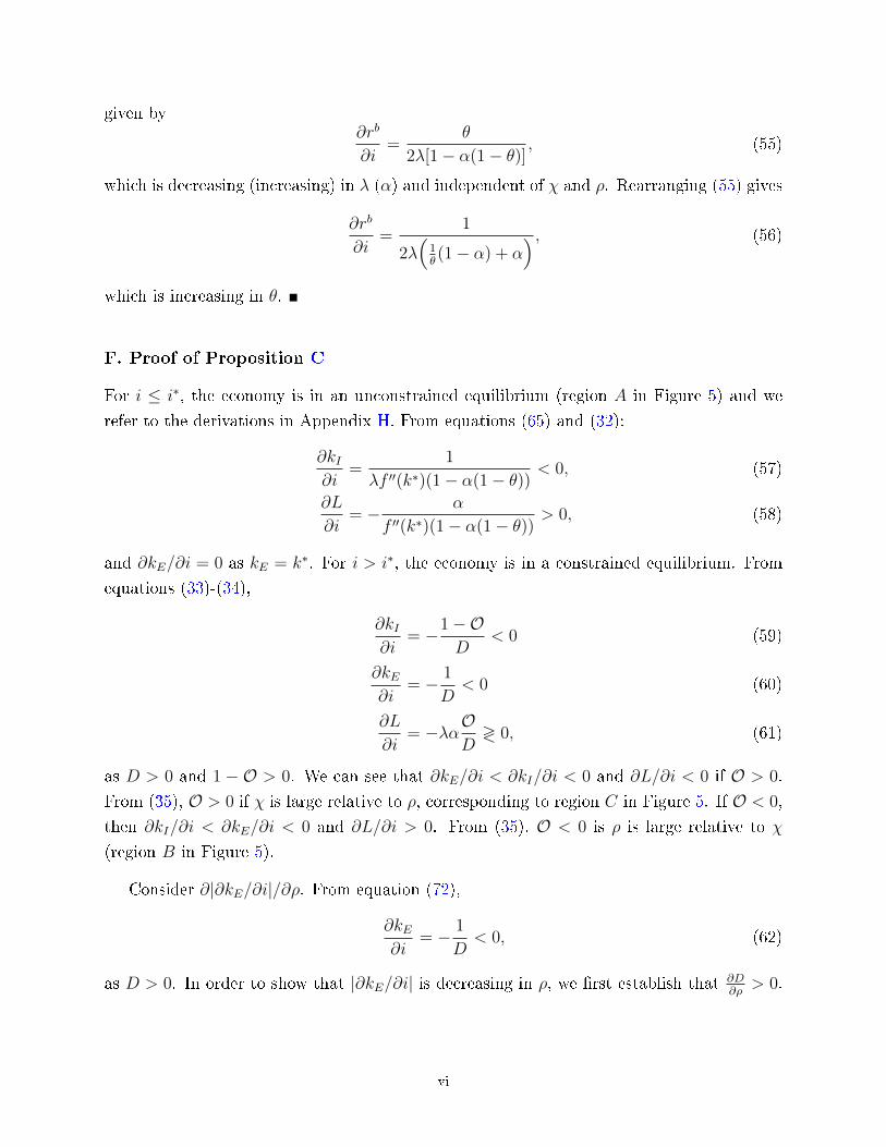
F. Proof of Proposition C

For i ≤ i∗, the economy is in an unconstrained equilibrium (region A in Figure 5) and we

refer to the derivations in Appendix H. From equations (65) and (32):

∂kI∂i

=1

λf ′′(k∗)(1− α(1− θ)) < 0, (57)

∂L

∂i= − α

f ′′(k∗)(1− α(1− θ)) > 0, (58)

and ∂kE/∂i = 0 as kE = k∗. For i > i∗, the economy is in a constrained equilibrium. From

equations (33)-(34),

∂kI∂i

= −1−OD

< 0 (59)

∂kE∂i

= − 1

D< 0 (60)

∂L

∂i= −λαO

D≷ 0, (61)

as D > 0 and 1 − O > 0. We can see that ∂kE/∂i < ∂kI/∂i < 0 and ∂L/∂i < 0 if O > 0.

From (35), O > 0 if χ is large relative to ρ, corresponding to region C in Figure 5. If O < 0,

then ∂kI/∂i < ∂kE/∂i < 0 and ∂L/∂i > 0. From (35), O < 0 is ρ is large relative to χ

(region B in Figure 5).

Consider ∂|∂kE/∂i|/∂ρ. From equation (72),

∂kE∂i

= − 1

D< 0, (62)

as D > 0. In order to show that |∂kE/∂i| is decreasing in ρ, we �rst establish that ∂D∂ρ

> 0.

vi

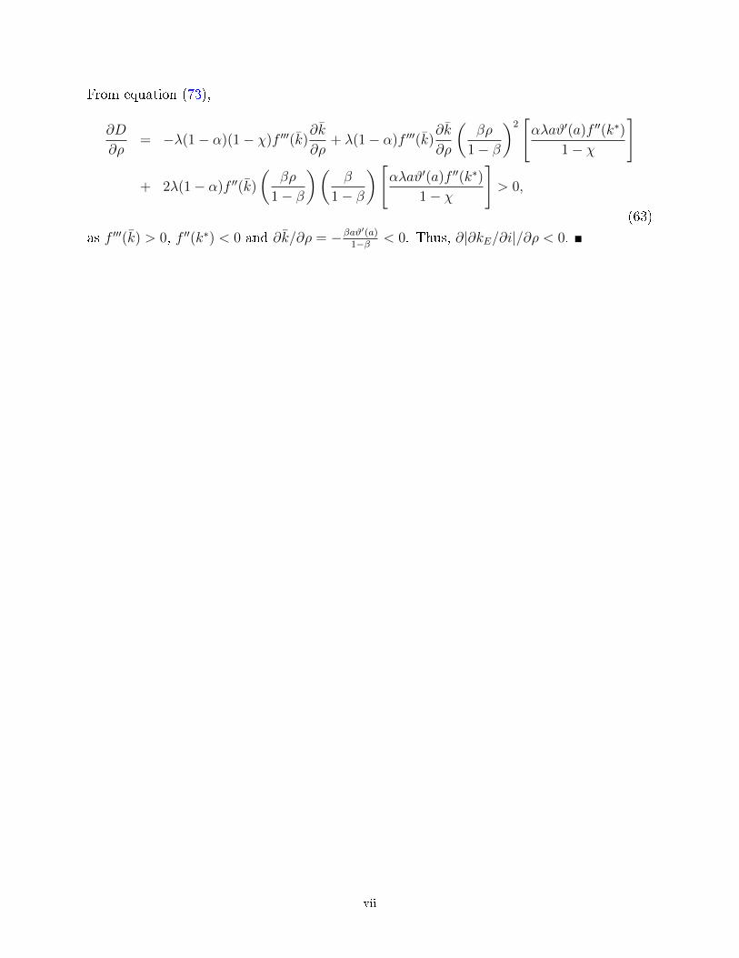
From equation (73),

∂D

∂ρ= −λ(1− α)(1− χ)f ′′′(k̄)

∂k̄

∂ρ+ λ(1− α)f ′′′(k̄)

∂k̄

∂ρ

(βρ

1− β

)2[αλaϑ′(a)f ′′(k∗)

1− χ

]

+ 2λ(1− α)f ′′(k̄)

(βρ

1− β

)(β

1− β

)[αλaϑ′(a)f ′′(k∗)

1− χ

]> 0,

(63)

as f ′′′(k̄) > 0, f ′′(k∗) < 0 and ∂k̄/∂ρ = −βaϑ′(a)1−β < 0. Thus, ∂|∂kE/∂i|/∂ρ < 0.

vii

Appendix: Supplementary Material

G. Data sources and construction

In the calibration of Section 7, our measure for the nominal interest (bank lending)

rate was the 3-month T-bill secondary market (bank prime) rate. Our measure of α, the

probability to receive a bank loan, follows from Rocheteau et al. (2018) who found that

between 78 − 90% of respondents in the 2003 Survey of Small Business Finances had their

most recent loan application approved. To calculate the pledgeability of output, we �rst

calculated the average of (i) total loans to non-�nancial non-corporate businesses and (ii)

total loans to non-�nancial non-corporate businesses net total home equity loans. We then

divide the amount of loans to non-�nancial non-corporate businesses by total assets among

non-�nancial non-corporate businesses. Both the data on loans and assets among non-

�nancial non-corporate businesses come from the Flow of Funds Accounts, where we use

quantities from Q4 in each year.

Our calculation of the pledgeability of housing, ρ, and maximum amount of unsecured

credit, b, draws on data from (i) the Federal Reserve Bank of New York's Quarterly Report

on Household Debt and Credit and (ii) Average Sales Price of Houses Sold for the United

States from the Federal Reserve Bank of St. Louis' FRED data base (series ASPUS). To

calculate ρ, we �rst compute the average Home Equity Revolving Limit by dividing the total

amount of Home Equity Revolving Limit by the number of Home Equity accounts between

2003:Q1-2016:Q4 using the FRBNY data. We then compute the ratio of the average home

equity limit to the average sale price of U.S. homes. To calculate b, we compute the average

credit limit by dividing the aggregate credit card limit by the number of credit card accounts

in the FRBNY data between 2003:Q1-2016:Q4. We then compute the average ratio of credit

limits to home equity loan limits and choose b so the ratio of the maximum amount of

unsecured credit relative to the maximum home equity loan in the model corresponds to the

same ratio in the data.

Last but not least, we estimated the probability of receiving an investment opportunity,

λ, by using data from the SCF between 2001-2016. Speci�cally, we calculated the fraction

of respondents who started or acquired their business within the last year.17

17Our calculation uses sample weights provided by the SCF.

viii

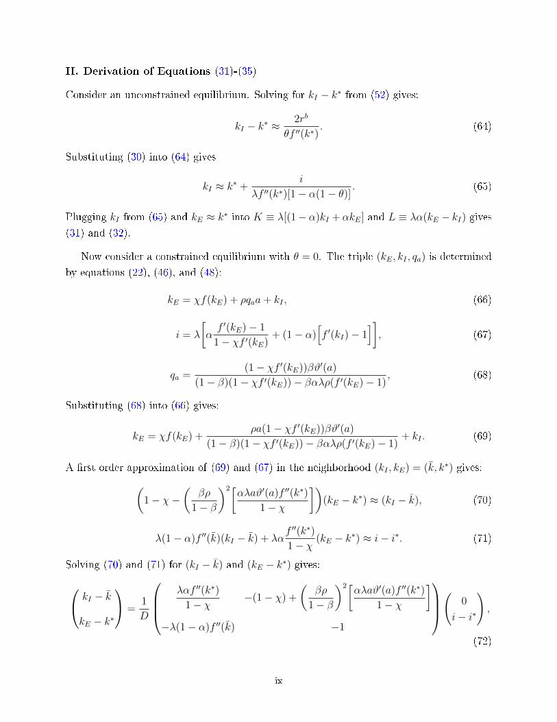
H. Derivation of Equations (31)-(35)

Consider an unconstrained equilibrium. Solving for kI − k∗ from (52) gives:

kI − k∗ ≈2rb

θf ′′(k∗). (64)

Substituting (30) into (64) gives

kI ≈ k∗ +i

λf ′′(k∗)[1− α(1− θ)] . (65)

Plugging kI from (65) and kE ≈ k∗ into K ≡ λ[(1− α)kI + αkE] and L ≡ λα(kE − kI) gives(31) and (32).

Now consider a constrained equilibrium with θ = 0. The triple (kE, kI , qa) is determined

by equations (22), (46), and (48):

kE = χf(kE) + ρqaa+ kI , (66)

i = λ

[αf ′(kE)− 1

1− χf ′(kE)+ (1− α)

[f ′(kI)− 1

]], (67)

qa =(1− χf ′(kE))βϑ′(a)

(1− β)(1− χf ′(kE))− βαλρ(f ′(kE)− 1), (68)

Substituting (68) into (66) gives:

kE = χf(kE) +ρa(1− χf ′(kE))βϑ′(a)

(1− β)(1− χf ′(kE))− βαλρ(f ′(kE)− 1)+ kI . (69)

A �rst order approximation of (69) and (67) in the neighborhood (kI , kE) = (k̄, k∗) gives:(1− χ−

(βρ

1− β

)2[αλaϑ′(a)f ′′(k∗)

1− χ

])(kE − k∗) ≈ (kI − k̄), (70)

λ(1− α)f ′′(k̄)(kI − k̄) + λαf ′′(k∗)

1− χ (kE − k∗) ≈ i− i∗. (71)

Solving (70) and (71) for (kI − k̄) and (kE − k∗) gives: kI − k̄

kE − k∗

=1

D

λαf ′′(k∗)

1− χ −(1− χ) +

(βρ

1− β

)2[αλaϑ′(a)f ′′(k∗)

1− χ

]−λ(1− α)f ′′(k̄) −1

(

0

i− i∗

),

(72)

ix

where

D = −λαf′′(k∗)

1− χ − λ(1− α)f ′′(k̄)

((1− χ)−

(βρ

1− β

)2[αλaϑ′(a)f ′′(k∗)

1− χ

])> 0, (73)

gives kI and kE. Finally, using L ≡ λα(kE − kI) and substituting kI and kE gives (34).

x