Entrepreneurial Finance and Non-diversifiable Risk∗

Hui Chen† Jianjun Miao‡ Neng Wang§

March 25, 2009

Abstract

Entrepreneurs face significant non-diversifiable business risks. We build a dynamic incomplete-markets model of entrepreneurial finance to demonstrate the important implications of non-diversifiable risks for entrepreneurs’ interdependent consumption, portfolio allocation, financ-ing, investment, and business exit decisions. The optimal capital structure is determined by ageneralized tradeoff model where leverage via risky non-recourse debt provides significant diversi-fication benefits. More risk-averse entrepreneurs default earlier, but also choose higher leverage,even though leverage makes his equity more risky. Non-diversified entrepreneurs demand bothsystematic and idiosyncratic risk premium. Cash-out option and external equity further improvediversification and raise the entrepreneur’s valuation of the firm. Finally, entrepreneurial riskaversion can overturn the risk-shifting incentives induced by risky debt.

Keywords: Default, diversification benefits, entrepreneurial risk aversion, incomplete markets,private equity premium, hedging, capital structure, cash-out option, precautionary saving

JEL Classification: G11, G31, E2

∗We thank Yakov Amihud, Patrick Bolton, John Cox, Bob Hall, Glenn Hubbard, Larry Kotlikoff, Debbie Lucas,Morten Sorensen, and seminar participants at Baruch, Boston University, Colorado, Columbia, Kansas, Michigan,MIT, Conference on Financial Innovation: 35 Years of Black/Scholes and Merton at Vanderbilt University, and NYUStern for comments. Jianjun Miao gratefully acknowledges financial support from Research Grants Council of HongKong under the project number 643507. Part of this research was conducted when Jianjun Miao was visiting HongKong University of Science and Technology. The hospitality of this university is gratefully acknowledged.

†MIT Sloan School of Management, 50 Memorial Drive, Cambridge, MA 02142. Email: huichen@mit.edu. Tel.:617-324-3896.

‡Department of Economics, Boston University, 270 Bay State Road, Boston, MA 02215. Email: miaoj@bu.edu.Tel.: 617-353-6675.

§Columbia Business School and National Bureau of Economic Research. Address: Columbia Business School,3022 Broadway, Uris Hall 812, New York, NY 10027. Email: neng.wang@columbia.edu. Tel.: 212-854-3869.

1 Introduction

Entrepreneurship plays an important role in fostering innovation and economic growth (Schum-

peter (1934)). For reasons such as incentive alignment and informational asymmetry between

the entrepreneur and financiers, entrepreneurs typically hold a significant non-diversified equity

position in their businesses, and thus bear non-diversifiable entrepreneurial business risk.1 For

example, using data from the survey of consumer finance, Gentry and Hubbard (2004) report that

active businesses on average account for 41.5 percent of entrepreneurs’ total assets. Moskowitz

and Vissing-Jorgensen (2002) document that about 75 percent of all private equity is owned by

households for whom it constitutes at least half of their total net worth.

Entrepreneurs are both producers and consumers. Like firms, they need to make invest-

ment/capital budgeting, financing, and business exit decisions. Like consumers, they also man-

age household finance and have preferences for intertemporal consumption smoothing. The non-

diversifiable idiosyncratic risk that the entrepreneurs bear from their businesses makes the business

decisions and household decisions interdependent. We integrate intertemporal household finance

(consumption-smoothing, portfolio choice) with corporate finance, and provide a utility-maximizing

framework to analyze the entrepreneurial firm’s capital budgeting/investment, capital structure,

and business exit decisions.

We model an infinitely-lived risk-averse entrepreneur who has access to an illiquid non-tradable

investment project. The project requires a lump-sum investment to start up, and generates stochas-

tic cash flows that bear both systematic and idiosyncratic risks. If he chooses to take on the project,

the entrepreneur sets up a firm with limited liability.

Our baseline model analyzes the tradeoff between inside equity and external risky debt. Our

focus on this tradeoff is motivated by the following empirical evidence. Heaton and Lucas (2004)

document the high concentration of equity ownership in entrepreneurial firms and the importance

of debt as a source of outside funding using data from the Survey of Small Business Finances

(SSBF). For example, they report that the principal owner holds on average 81 percent of the

firm’s equity, and the median owner wholly owns the firm. These findings are consistent with

results from earlier Fed surveys of small businesses, as reported in Berger and Udell (1998), Cole

and Wolken (1996), and Petersen and Rajan (1994). Using a large data set of public and private

1Bitler, Moskowitz and Vissing-Jorgensen (2005) provide evidence that agency considerations play a key role inexplaining why entrepreneurs on average hold large ownership shares.

1

firms in the United Kingdom, Brav (2009) finds that private firms rely almost exclusively on debt

financing, have higher leverage ratios, and tend to avoid external capital markets, compared to

their public counterparts. Furthermore, Leland and Pyle (1977) show that debt often dominates

equity in settings with asymmetric information because debt is less information-sensitive.

After the firm is set up, the entrepreneur decides when to default on his debt (if the business does

sufficiently poorly), and when to cash out by selling the firm (if the business is doing sufficiently

well). In addition to the business exit decisions, he also chooses consumption and allocates his

liquid wealth between a riskless asset and a diversified market portfolio (as in Merton (1971)).

While the entrepreneur can hedge the systematic component of his business risks using the

market portfolio, he cannot diversify the idiosyncratic risks. Moreover, both default and cashing

out options are costly. Therefore, the entrepreneur faces incomplete markets, and the idiosyncratic

risk exposure has important effects on the entrepreneur’s interdependent consumption, investment,

financing, and business exit decisions.

While the entrepreneur can hedge the systematic component of his business risks using the

market portfolio, he cannot diversify the idiosyncratic risks. Moreover, exit via default or cashing

out is costly. Therefore, the entrepreneur faces incomplete markets, and the idiosyncratic risk

exposure will have important effects on the entrepreneur’s interdependent consumption, investment,

financing, and business exit decisions.

Our main results are as follows. The default option embedded in non-recourse debt allows the

entrepreneur to limit his liability when walking away from his business. Intuitively, the entrepreneur

is long a default (put) option (i.e., a state-contingent sale of the firm to the financier), which is an

insurance to the entrepreneur against the firm’s potential poor performance in the future. Because

the entrepreneur is exposed to the idiosyncratic risk from his concentrated ownership position in the

firm, the diversification benefits of external risky debt are important when markets are incomplete.

The diversification benefits of debt are large. Even without the tax benefits of debt, the en-

trepreneurial firm still issues a significant amount of debt. The diversification benefits also lead to

a seemingly counterintuitive prediction: more risk-averse entrepreneurs choose higher leverage. On

the one hand, higher leverage increases the risk for the entrepreneur’s equity stake. On the other

hand, higher leverage/debt implies less equity exposure to the entrepreneurial project, making the

entrepreneur’s overall portfolio (including both his private equity in the firm and his liquid finan-

cial wealth) less risky. This overall portfolio composition effect dominates the high leverage effect

2

within the firm. The more risk-averse the entrepreneur, the stronger the need to reduce his firm

risk exposure, therefore the higher the leverage.

The non-diversifiable risk and concentrated wealth in the business make the entrepreneur value

his equity less than do diversified investors. The entrepreneur demands an extra premium for bear-

ing the idiosyncratic risks of the firm. Thus, compared to a well-diversified firm, the entrepreneur

tends to default earlier on his debt. While equity is a call option on firm assets, and hence is convex

in firm cash flows, in our model, the private value of equity is not necessarily globally convex. When

risk aversion and/or idiosyncratic volatility are sufficiently high, the entrepreneur’s precautionary

saving demand can make his private value of equity concave in cash flow.

This finding has important implications for risk shifting, an agency problem induced by risky

debt. Jensen and Meckling (1976) point out that managers of public firms have incentives to invest

in excessively risky projects after debt is in place because of the convexity feature of equity. In our

model, when the degree of risk aversion is high enough, the entrepreneur’s private value of equity

(locally) decreases with the idiosyncratic volatility of the project. Thus, he may prefer to invest in

a low idiosyncratic volatility project with debt in place, overturning the asset substitution result of

Jensen and Meckling (1976). We find that, when the firm is not in distress, very low risk aversion

is enough to make the entrepreneur prefer safer projects. Our model thus provides a potential

explanation for the lack of empirical and survey evidence on asset substitution and risk-shifting

incentives.

The standard option valuation analysis is no longer applicable to the default and cash-out op-

tions in our setting because these options are non-tradable and their underlying assets are illiquid.

Under the assumption of constant absolute risk aversion (CARA) utility, we provide an analytically

tractable framework to value these options. We also derive an analytical formula for the idiosyn-

cratic risk premium demanded by the entrepreneur. The key determinants of the idiosyncratic risk

premium are risk aversion, idiosyncratic volatility, and the sensitivity of entrepreneurial value of

equity with respect to cash flow. The dynamic properties of the idiosyncratic risk premium are

quite different from the systematic risk premium, especially when the firm is close to default or

cash-out. Moreover, ignoring the idiosyncratic risk premium can lead to substantial downward bias

in the estimates of the leverage ratio of entrepreneurial firms.

Finally, we extend our model to allow the entrepreneur to issue costly external equity. The more

external equity issued, the smaller the entrepreneur’s idiosyncratic risk exposure, but it also creates

3

an incentive problem for the entrepreneur, which lowers the expected growth rate of revenue. We

show that the entrepreneur’s dependence on external debt for diversification decreases when he has

access to external equity. Intuitively, external equity is more effective than debt in transferring

idiosyncratic risks to outside investors. The entrepreneur maximizes his ex ante private value of

the firm by trading off the diversification benefits of equity against the costs of incentive problems.

This paper builds on the insight of Heaton and Lucas (2004), who are the first to model the

diversification benefits of risky debt in a static model with asymmetric information (as in Leland and

Pyle (1977)). We study the entrepreneur’s consumption, portfolio choice, (debt/equity) financing,

and exit (default/cash-out) decisions in a dynamic trade-off model. Our model is tractable and

allows for analytical characterization of the dynamics of debt, equity, and the systematic and

idiosyncratic risk premium demanded by the entrepreneur. We also incorporate a range of realistic

features for entrepreneurial financing, including taxes, cash-out options, and external equity.

We integrate incomplete markets and diversification benefits into the tradeoff model of Le-

land (1994), thus bringing a new dimension to the structural credit risk/capital structure models.2

Our generalized tradeoff model not only applies to entrepreneurs, but also to public firms with

under-diversified managers. Our model is related to the incomplete-markets consumption smooth-

ing/precautionary saving literature.3 For analytical tractability reasons, we adopt the CARA utility

specification as in Merton (1971), Caballero (1991), Kimball and Mankiw (1989), and Wang (2006).

Our model contributes to this literature by extending the CARA-utility-based precautionary saving

problem to allow the entrepreneur to reduce his idiosyncratic risk exposure via exit strategies such

as cash-out and default.

This paper is also related to the real options literature.4 The closest paper is Miao and Wang

(2007), who analyze the impact of the entrepreneur’s non-diversifiable idiosyncratic risks on his

growth option exercising decision. The present paper analyzes the entrepreneurial firm’s investment

and financing (internal versus external, debt versus equity), and endogenous default and cash-out

decisions.

2See Leland (1994), Goldstein, Ju, and Leland (2001), Strebulaev (2007), Hackbarth, Miao, and Morellec (2006),Bhamra, Kuehn, and Strebulaev (2008), Chen (2008), and earlier work of Black and Cox (1976), and Fischer, Heinkel,and Zechner (1989).

3Hall (1978) initiated the Euler equation approach to study intertemporal consumption behavior. See Deaton(1992) and Attanasio (1999) for surveys.

4See Brennan and Schwartz (1986), McDonald and Siegel (1986), Abel and Eberly (1994), and Dixit and Pindyck(1994).

4

2 Model setup

Investment opportunities An infinitely-lived risk-averse agent has a take-it-or-leave-it project

at time 0, which requires a one-time investment I. The project generates a stochastic revenue

process {yt : t ≥ 0} that follows a geometric Brownian motion (GBM):

dyt = µytdt + ωytdBt + ǫytdZt, y0 given, (1)

where µ is the expected growth rate of the revenue, Bt and Zt are independent standard Brownian

motions, which are the sources of market (systematic) and idiosyncratic risks of the private business,

respectively. The parameters ω and ǫ are the systematic and idiosyncratic volatility parameters of

the revenue growth. The total volatility of revenue growth is

σ =√

ω2 + ǫ2. (2)

As we will show, these different volatility parameters ω, ǫ, and σ have different effects on the

entrepreneur’s decision making.

In addition, the agent has access to standard financial investment opportunities as in Merton

(1971).5 The agent allocates his liquid financial wealth between a riskfree asset which pays a

constant rate of interest r and a diversified market portfolio (the risky asset) with returns Rt

satisfying:

dRt = µpdt+ σpdBt, (3)

where µp and σp are the expected return and volatility of the risky asset, respectively, and Bt is

the standard Brownian motion introduced earlier. Let

η =µp − r

σp(4)

denote the after-tax Sharpe ratio of the market portfolio, and let {xt : t ≥ 0} denote the en-

trepreneur’s liquid (financial) wealth process. The entrepreneur invests the amount φt in the

market portfolio (the risky asset) and the remaining amount xt − φt in the riskfree asset.

Entrepreneurial firm If the entrepreneur decides to start the project, he runs it by setting up

a limited-liability entity, such as a limited liability company (LLC) or an S corporation. The LLC

5It is straightforward to consider entering the labor market as an alternative to running entrepreneurial business,which provides an endogenous opportunity cost of taking on the entrepreneurial project. Such an extension does notchange key economics of our paper in any significant way.

5

or S corporation allows the entrepreneur to face single-layer taxation for his business income and

makes the debt non-recourse. We may extend the model to allow for personal guarantee of debt to

varying degrees. This feature effectively makes debt recourse to varying degrees. The entrepreneur

finances the initial one-time lump-sum cost I via his own funds (internal financing) and external

financing. In the benchmark case, we assume that the only source of external financing is debt. See

Petersen and Rajan (2002), Heaton and Lucas (2004), and Brav (2009) for evidence that debt is

the primary source of financing for most entrepreneurial firms.6 One interpretation of the external

debt is bank loans. The entrepreneur uses the firm’s assets as collateral to borrow, so that the debt

is secured.

We assume that debt is issued at par and is interest-only (consol) for tractability reasons as

in Leland (1994) and Duffie and Lando (2001). Let b denote the coupon payment of debt and F0

denote the par value of debt. Debt is priced competitively in that the lender breaks even on the

risk-adjusted basis. We further assume that debt is only issued at time 0 and remains unchanged

until the entrepreneur exits. Allowing for dynamic capital structure before exit will not change

the key economic tradeoff that we focus on: the impact of idiosyncratic risk on entrepreneurial

financing decisions.

After debt is in place, at any time t > 0, the entrepreneur has three choices: (1) continuing

his business; (2) defaulting on the outstanding debt, which leads to the liquidation of his firm; (3)

cashing out by selling the firm to a diversified buyer.

While running the business, the entrepreneur receives income from the firm in the form of

cash payments (operating profit net of coupon payments). Negative cash payments are interpreted

as cash injections by the entrepreneur into the firm. Notice that trading riskless bonds and the

diversified market portfolio alone does not help the entrepreneur diversify the idiosyncratic business

risk. He can sell the firm and cash out, which requires a fixed transaction cost K. The default

timing Td and cash-out timing Tu are not contractible at time 0. Instead, the entrepreneur chooses

the default/cash-out policy to maximize his own utility after he chooses the time-0 debt level. Thus,

there is an inevitable conflict of interest between financiers and the entrepreneur. The choices of

default and cash-out resemble American-style put and call options on the underlying non-tradeable

entrepreneurial firm. Since markets are incomplete for the entrepreneur, we cannot price the

entrepreneur’s options using the standard dynamic replication argument (Black-Scholes-Merton).

6In Section VII, we introduce external equity as an additional source of financing.

6

At bankruptcy, the outside lender takes control and liquidates/sells the firm. Bankruptcy ex post

is costly as in standard tradeoff models of capital structure. We assume that the liquidation/sale

value of the firm is equal to a fraction α of the value of an all equity (unlevered) public firm, A (y).

The remaining fraction (1 − α) is lost due to bankruptcy costs. We also assume that absolute

priority is enforced, and abstract away from any ex post renegotiation between the lender and the

entrepreneur.

Before the entrepreneur can sell the firm, he needs to retire the firm’s debt obligation at par

F0. We make the standard assumption that the buyer is well diversified. He will optimally relever

the firm as in the complete-markets model of Leland (1994). The value of the firm after sale is the

value of an optimally levered public firm, V ∗(y).

After the entrepreneur exits from his business (through default or cash-out), he “retires” and

lives on his financial income. He then faces a standard complete-markets consumption and portfolio

choice problem.7

Taxes We consider a simple tax environment. The entrepreneurial firm pays taxes on his business

profits at rate τe. When τe > 0, issuing debt has the benefit of shielding part of the entrepreneur’s

business profits from taxes. For a public firm, the effective marginal tax rate is τm. Unlike the

entrepreneurial firm, the public firm is subject to double taxation (at the corporate and individual

levels), and τm captures the net tax rate (following Miller (1977)). Finally, τg denotes the tax

rate on the capital gains upon sale. Naturally, higher capital gain taxes will delay the timing of

cash-out.

Entrepreneur’s objective The entrepreneur derives utility from consumption {ct : t ≥ 0} ac-

cording to the following time-additive utility function:

E

[∫ ∞

0e−δtu (ct) dt

]

, (5)

where δ > 0 is the entrepreneur’s subjective discount rate and u( · ) is an increasing and concave

function. The entrepreneur’s objective is to maximize his lifetime utility by optimally choosing

consumption (ct), financial portfolio (φt), and whether to start his business. If he starts his business,

he also chooses the financing structure of the firm (coupon b), and the subsequent timing decisions

of default and cash-out (Td, Tu).

7Extending our model to allow for sequential rounds of entrepreneurial activities will complicate our analysis. Weleave this extension for future research.

7

In general, incomplete markets imply that the entrepreneur cannot fully diversify his business

risk and hence cannot fully separate his investment from consumption decisions. Indeed, provided

that u′(c) is convex, the entrepreneur’s precautionary motive will determine his intertemporal

consumption smoothing.8

3 Model solution

First, in Section III.A, we report the complete-markets solution for firm value and financing de-

cisions when the firm is owned by diversified investors. Then, we analyze the entrepreneur’s in-

terdependent consumption/saving, portfolio choice, default, and initial investment and financing

decisions. The complete-markets solution of Section III.A serves as a natural benchmark for us to

analyze the impact of non-diversifiable idiosyncratic risk on entrepreneurial investment, financing

and valuation.

3.1 Complete-markets firm valuation and financing policy

Consider a public firm owned by diversified investors. Because equityholders internalize the benefits

and costs of debt issuance, they will choose the firm’s debt policy to maximize ex ante firm value

by trading off the tax benefits of debt against bankruptcy and agency costs. The results in this

case are well-known.9 In Appendix A, we provide the after-tax value of an unlevered public firm

A(y) in equation (A.19), and the after-tax value of a public levered firm V ∗(y) in equation (A.21).

Next, we turn to analyze the entrepreneur’s decision problem before he exits from his business.

3.2 Entrepreneur’s problem

The significant lack of diversification invalidates the standard finance textbook valuation analysis for

firms owned by diversified investors. As a result, the standard two-step complete-markets (Arrow-

Debreu) analysis10 (i.e., first value maximization and then optimal consumption allocation) no

longer applies. This non-separability between value maximization and consumption smoothing has

important implications for real economic activities (e.g., investment and capital budgeting) and the

valuation of claims that an entrepreneur issues to finance his investment activities.

8Leland (1968) is among the earliest studies on precautionary saving models. Kimball (1990) links the degree ofprecautionary saving to the convexity of the marginal utility function u′(c).

9For example, see Leland (1994), Goldstein, Ju, and Leland (2001), and Miao (2005).10Cox and Huang (1989) apply this insight to separate intertemporal portfolio choices from consumption in

continuous-time diffusion settings.

8

We solve the entrepreneur’s problem by backward induction. First, we summarize the en-

trepreneur’s consumption/saving and portfolio choice problem after he retires from his business via

either cashing out or defaulting on debt. This “retirement-stage” optimization problem is the same

as in Merton (1971), a dynamic complete-markets consumption/portfolio choice problem. Second,

we solve the entrepreneur’s joint consumption/saving, portfolio choice, and default decisions when

the entrepreneur runs his private business. Third, we determine the entrepreneur’s exit decisions

(his cash-out and default boundaries) by comparing his value functions just before and after re-

tirement. Finally, we solve the entrepreneur’s initial (time-0) investment and financing decisions

taking his future decisions into account.

Conceptually, our model setup applies to any utility function u(c) under technical regularity

conditions. For analytical tractability, we adopt the CARA utility throughout the remainder of

the paper.11 That is, let u (c) = −e−γc/γ, where γ > 0 is coefficient of absolute risk aversion,

which also measures precautionary motive. We emphasize that the main results and insights of

our paper (the effect of non-diversifiable idiosyncratic shocks on investment timing) do not rely

on the choice of this utility function. As we show below, the driving force of our results is the

precautionary savings effect, which is captured by utility functions with convex marginal utility such

as CARA. While CARA utility does not capture wealth effects, it helps reduce the dimension of our

double-barrier free-boundary problem, which makes the problem much more tractable compared

to constant relative risk aversion (CRRA) utility.

Consumption/saving and portfolio choice after exit. After exiting from his business (via

either default or cash-out), the entrepreneur no longer has any business income, and lives on his

financial wealth. The entrepreneur’s optimization problem becomes the standard complete-market

consumption and portfolio choice problem (e.g., Merton (1971)). We summarize the results in

Appendix B.

Entrepreneur’s decision making while running the firm. We summarize the solution for

consumption/saving, portfolio choice, default trigger yd, and cash-out trigger yu in the following

theorem.

11The CARA utility specification proves tractable in incomplete-markets consumption-saving problems with laborincome. Kimball and Mankiw (1989), Caballero (1991), Svensson and Werner (1993), and Wang (2006) have alladopted this utility specification in various precautionary saving models. Miao and Wang (2007) use this utilityspecification to analyze a real option exercising problem when the decision maker faces uninsurable idiosyncratic riskfrom his investment opportunity.

9

Theorem 1 The entrepreneur exits from his business when the revenue process {yt : t ≥ 0} reaches

either the default threshold yd or the cash-out threshold yu, whichever comes first. Prior to exit,

for given liquid wealth x and revenue y, he chooses his consumption and portfolio rules as follows:

c (x, y) = r

(

x+G (y) +η2

2γr2+δ − r

γr2

)

, (6)

φ (x, y) =η

γrσp−ω

σpyG′ (y) , (7)

where G(·) and yd solve the free boundary problem given by the differential equation:

rG(y) = (1 − τe) (y − b− w) + (µ− ωη)yG′(y) +σ2y2

2G′′(y) −

γrǫ2y2

2G′(y)2, (8)

subject to the following (free) boundary conditions:

G(yd) = 0 (9a)

G′(yd) = 0 (9b)

G(yu) = V ∗ (yu) − F0 −K − τg (V ∗ (yu) −K − I) (9c)

G′(yu) = (1 − τg)V∗′ (yu) (9d)

where complete-markets firm value V ∗(y) is defined in (A.21), and the value of external debt F0 =

F (y0) is given in (C.6).

Equation (6) states that consumption is equal to the annuity value of the sum of financial wealth

x, certainty equivalent wealth G(y), and two constant terms capturing the effects of the expected

excess returns and the wedge δ−r on consumption. The key is to note that G(y) is the risk-adjusted

subjective valuation of the entrepreneur’s business project. Equation (7) gives the entrepreneur’s

portfolio holding, where the first term is the standard mean-variance term as in Merton (1971),

and the second term gives the entrepreneur’s hedging demand as he uses the market portfolio to

dynamically hedge the entrepreneurial business risk.

The differential equation (8) provides a valuation equation for the certainty equivalent wealth

G(y) from the entrepreneur’s perspective. In the standard CAPM model, only systematic risk

demands a risk premium under the complete-markets setting. Since the systematic volatility of

revenue growth is ω, the risk-adjusted expected growth rate of revenue in the CAPM model is

ν = µ− ωη. (10)

10

If we drop the last nonlinear term in (8), the differential equation becomes the standard pricing

equation: setting the instantaneous expected return of an asset under the risk-neutral measure

(RHS) equal to the riskfree rate (LHS). The last term in (8) captures the additional discount due

to the non-diversifiable idiosyncratic risk. Intuitively, the higher the risk aversion parameter γ or

the idiosyncratic volatility ǫy, the larger the discount on G(y) due to idiosyncratic risk. The next

section provides more detailed analysis on the impact of idiosyncratic risk on G(y).

Equation (9a) comes from the value-matching condition for the entrepreneur’s default decision.

It states that the private value of equity G(y) upon default is equal to zero. Equation (9b), often

referred to as the smooth-pasting condition, can be interpreted as the optimality condition for the

entrepreneur in choosing default.

Now we turn to the cash-out boundary. Because the entrepreneur pays the fixed cost K and

triggers capital gains when cashing out, he naturally has incentive to wait before cashing out. How-

ever, waiting also reduces his diversification benefits ceteris paribus. The entrepreneur optimally

trades off tax implications, diversification benefits, and transaction costs when choosing the timing

of cashing out. The value-matching condition (9c) at the cash-out boundary states that the private

value of equity upon the firm’s cashing out is equal to the after-tax value of the public firm value

after the entrepreneur pays the fixed costs K, retires outstanding debt at par F0, and pays capital

gains taxes. The smooth-pasting condition (9d) ensures that the entrepreneur optimally chooses

his cash-out decision.

Initial financing and investment decisions. Next, we complete the model solution by endo-

genizing the entrepreneur’s initial investment and financing decision. The entrepreneurial firm has

two financial claimants: inside equity (entrepreneur) and outside creditors. The entrepreneur val-

ues his ownership at a certainty equivalent value G(y). Diversified lenders price debt in competitive

capital markets at F (y), which does not contain the idiosyncratic risk premium because outside

investors are fully diversified. Thus, the total private value of the entrepreneurial firm is

S(y) = G(y) + F (y). (11)

We may interpret S(y) as the total value that an investor needs to pay in order to acquire the

entrepreneurial firm by buying out the entrepreneur and the debt investors.

At time 0, the entrepreneur thus chooses debt coupon b to maximize the private value of the

11

firm:

b∗ = argmaxb

S (y0; b) . (12)

Intuitively, the entrepreneur internalizes the benefits and costs of debt financing, and markets

competitively price the firm’s debt. In Appendix B, we show that (12) indeed arises from the

entrepreneur’s utility maximization problem stated in (B.18). Note the conflicts of interest between

the entrepreneur and external financiers. After debt is in place, the entrepreneur will no longer

maximize the total value of the firm S(y), but his private value of equity G(y). Theorem 1 has

already captured the conflict of interest between the entrepreneur and outside creditors.

The last step is to characterize whether the agent wants to undertake the project. He makes

the investment and starts up the firm at time 0 if his life-time utility with the project is higher

than that without the project. This is equivalent to the condition that S (y0) > I.

We may interpret our model’s implication on capital structure as a generalized tradeoff model

of capital structure for the entrepreneurial firm, where the entrepreneur trades off the benefits

of outside debt financing (diversification and potential tax implications) against the costs of debt

financing (bankruptcy and agency conflicts between the entrepreneur and outside lenders). The

natural measure of leverage from the entrepreneur’s point of view is the ratio between the public

value of debt F (y) and the private value of firm S(y),

L(y) =F (y)

S(y). (13)

We label L(y) as private leverage to reflect the impact of idiosyncratic risk on the leverage choice.

Note that the entrepreneur’s preferences (e.g., risk aversion) influence the firm’s capital structure.

The standard argument that shareholders can diversify for themselves and hence diversification

plays no role in the capital structure decisions of public firms is no longer valid for entrepreneurial

firms.

So far, we have focused on the parameter regions where the entrepreneur first establishes his

firm as a private business and finances its operation via an optimal mix of outside debt and inside

equity. We now point out two special cases. First, when the cost of cashing out is sufficiently

small, it is optimal for the entrepreneur to sell the firm immediately (yu = y0). The other special

case is when asset recovery rate is sufficiently high, or the entrepreneur is sufficiently risk averse,

so that he raises as much debt as possible and defaults immediately (yd = y0). Both cases lead to

immediate exit. In our analysis below, we consider parameter values that rule out these cases.

12

4 Risky debt, endogenous default, and diversification

We now investigate a special case of the model in Theorem 1 which highlights the diversification

benefits of risky debt. For this purpose, we shut down the cash-out option (by setting the cash-out

cost K to infinity, making the cash-out option worthless).

We use the following (annualized) baseline parameter values: riskfree interest rate r = 3%,

expected growth rate of revenue µ = 4%, systematic volatility of growth rate ω = 10%, idiosyncratic

volatility ε = 20%, market price of risk η = 0.4, and asset recovery rate α = 0.6. We set the

effective marginal Miller tax rate τm to 11.29% as in Graham (2000) and Hackbarth, Hennessy,

and Leland (2007).12 In our baseline parametrization, we set τe = 0, which reflects the fact that

the entrepreneur can avoid taxes on his business income completely by deducting various expenses.

Shutting down the tax benefits also allows us to highlight the diversification benefits of debt. Later,

we consider the case where τe = τm, which can be directly compared with the complete-markets

model. We set the entrepreneur’s rate of time preference δ = 3%, and consider three values of the

risk aversion parameter γ ∈ {0, 1, 2}. Finally, we set the initial level of revenue y0 = 1.

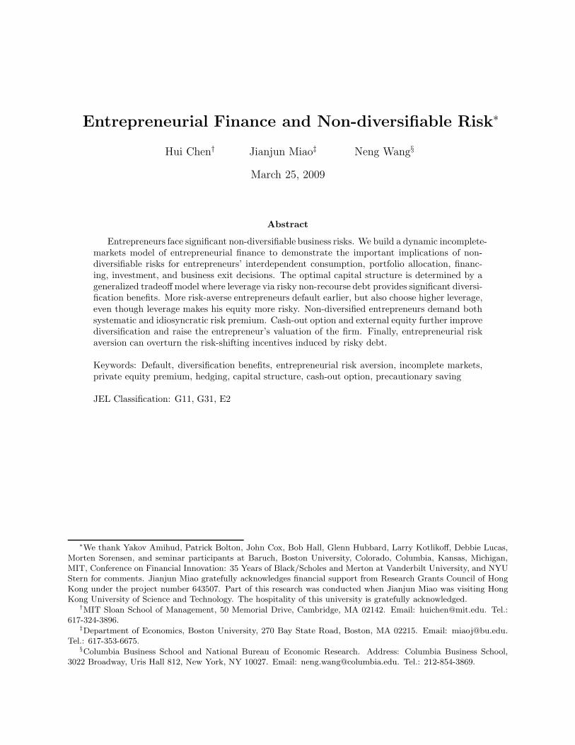
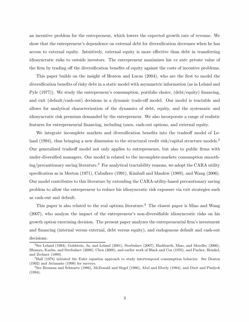
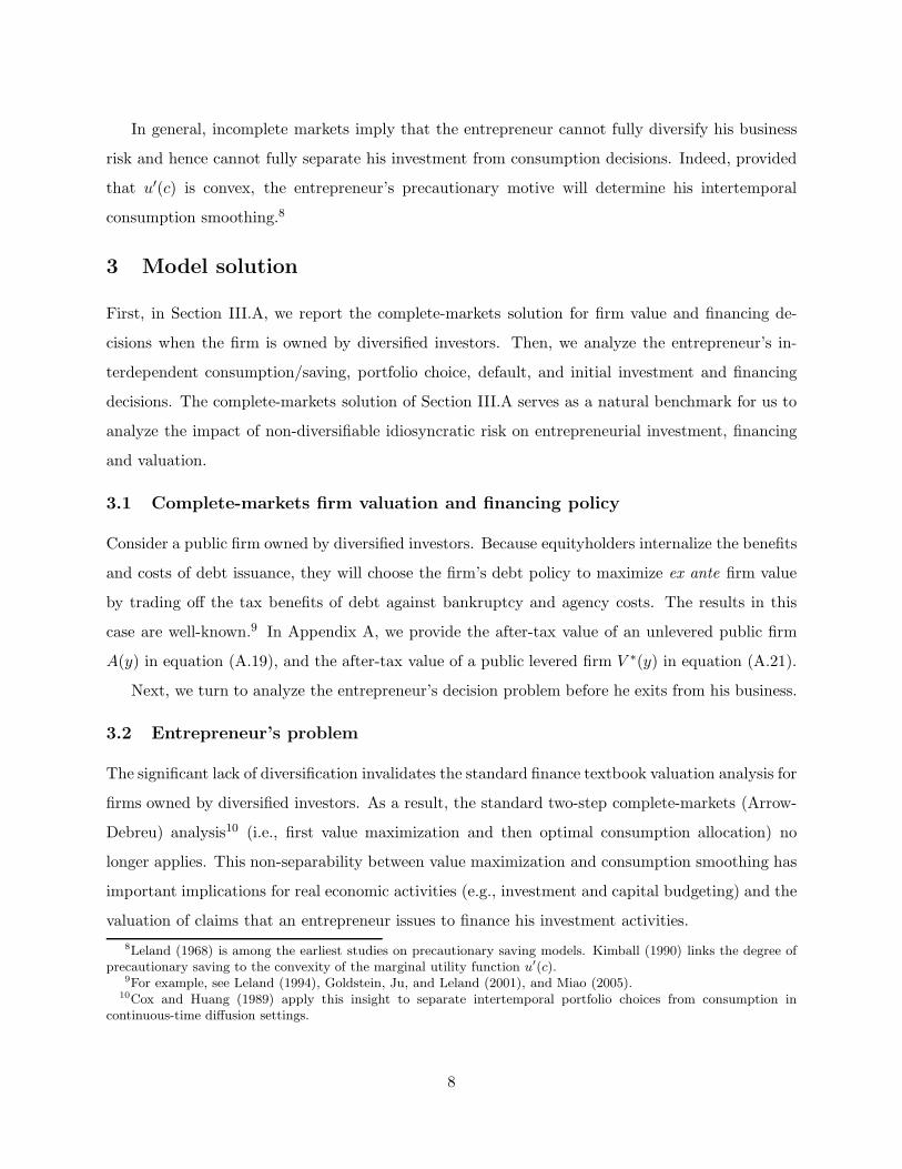
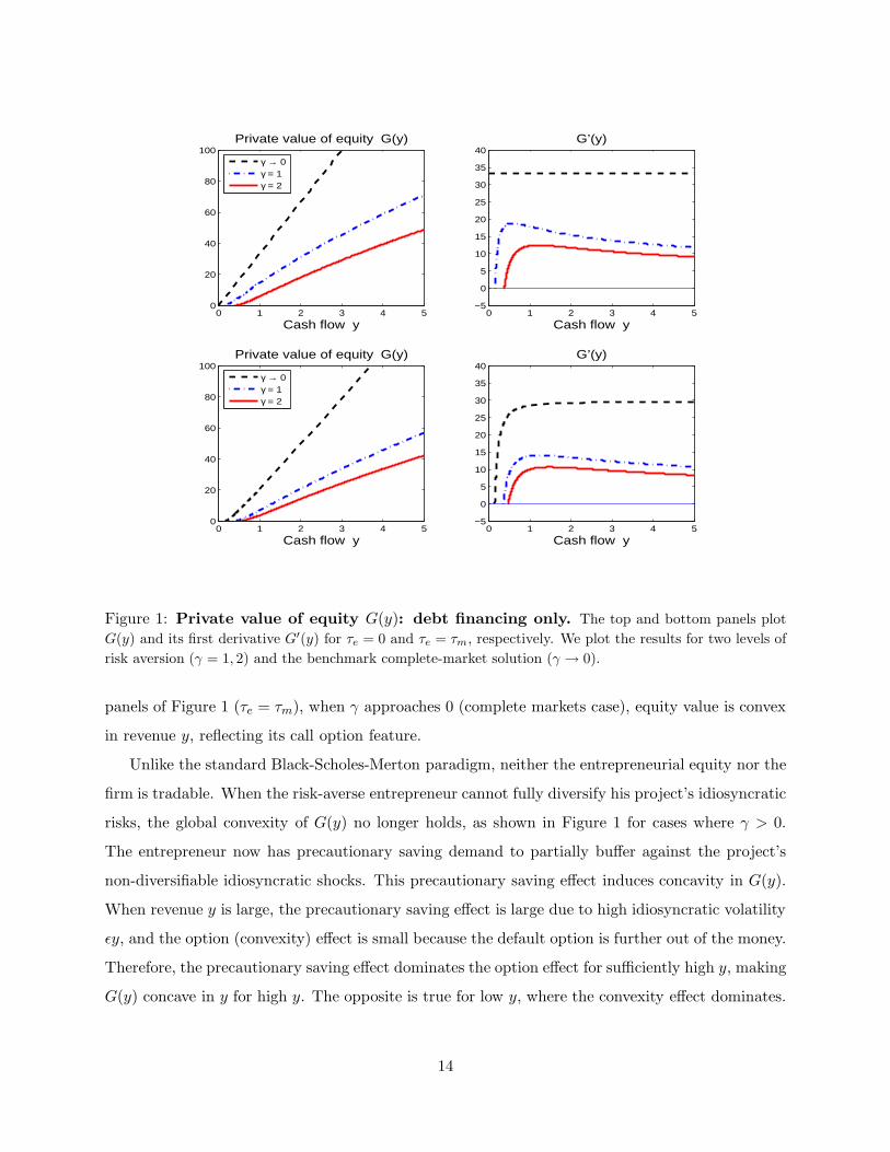
Private value of equity G(y) and default threshold. Figure 1 plots private value of equity

G(y) and its derivative G′ (y) as functions of y. The top and the bottom panels plot the results for

τe = 0 and τe = τm, respectively. When τe = 0, the entrepreneur with very low risk aversion (γ → 0,

effectively complete-markets) issues no debt, because there are neither tax benefits (τe = 0) nor

diversification benefits (γ → 0). Equity value is equal to the present discounted value of future cash

flows (the straight dash line shown in the top-left panel). A risk-averse entrepreneur has incentive

to issue debt in order to diversify idiosyncratic risks. The entrepreneur defaults when y falls to yd,

the point where G (yd) = G′ (yd) = 0. When τe = τm, the entrepreneurial firm issues debt to take

advantage of tax benefits in addition to diversification benefits. The bottom two panels of Figure

1 plot this case.

The derivative G′(y) measures the sensitivity of private value of equity G(y) with respect to

revenue y. As expected, private value of equity G(y) increases with revenue y, i.e., G′(y) > 0.

Analogous to Black-Scholes-Merton’s observation that firm equity is a call option on firm assets,

the entrepreneur’s private equity G(y) also has a call option feature. For example, in the bottom

12We may interpret τm as the effective Miller tax rate which integrates the corporate income tax, individual’sequity and interest income tax. Using the Miller’s formula for the effective tax rate , and setting the interest incometax at 0.30, corporate income tax at 0.31, and the individual’s long-term equity (distribution) tax at 0.10, we obtainan effective tax rate of 11.29%.

13

0 1 2 3 4 50

20

40

60

80

100

Cash flow y

Private value of equity G(y)

0 1 2 3 4 5−5

0

5

10

15

20

25

30

35

40G’(y)

Cash flow y

γ → 0γ = 1γ = 2

0 1 2 3 4 50

20

40

60

80

100

Cash flow y

Private value of equity G(y)

0 1 2 3 4 5−5

0

5

10

15

20

25

30

35

40G’(y)

Cash flow y

γ → 0γ = 1γ = 2

Figure 1: Private value of equity G(y): debt financing only. The top and bottom panels plot

G(y) and its first derivative G′(y) for τe = 0 and τe = τm, respectively. We plot the results for two levels of

risk aversion (γ = 1, 2) and the benchmark complete-market solution (γ → 0).

panels of Figure 1 (τe = τm), when γ approaches 0 (complete markets case), equity value is convex

in revenue y, reflecting its call option feature.

Unlike the standard Black-Scholes-Merton paradigm, neither the entrepreneurial equity nor the

firm is tradable. When the risk-averse entrepreneur cannot fully diversify his project’s idiosyncratic

risks, the global convexity of G(y) no longer holds, as shown in Figure 1 for cases where γ > 0.

The entrepreneur now has precautionary saving demand to partially buffer against the project’s

non-diversifiable idiosyncratic shocks. This precautionary saving effect induces concavity in G(y).

When revenue y is large, the precautionary saving effect is large due to high idiosyncratic volatility

ǫy, and the option (convexity) effect is small because the default option is further out of the money.

Therefore, the precautionary saving effect dominates the option effect for sufficiently high y, making

G(y) concave in y for high y. The opposite is true for low y, where the convexity effect dominates.

14

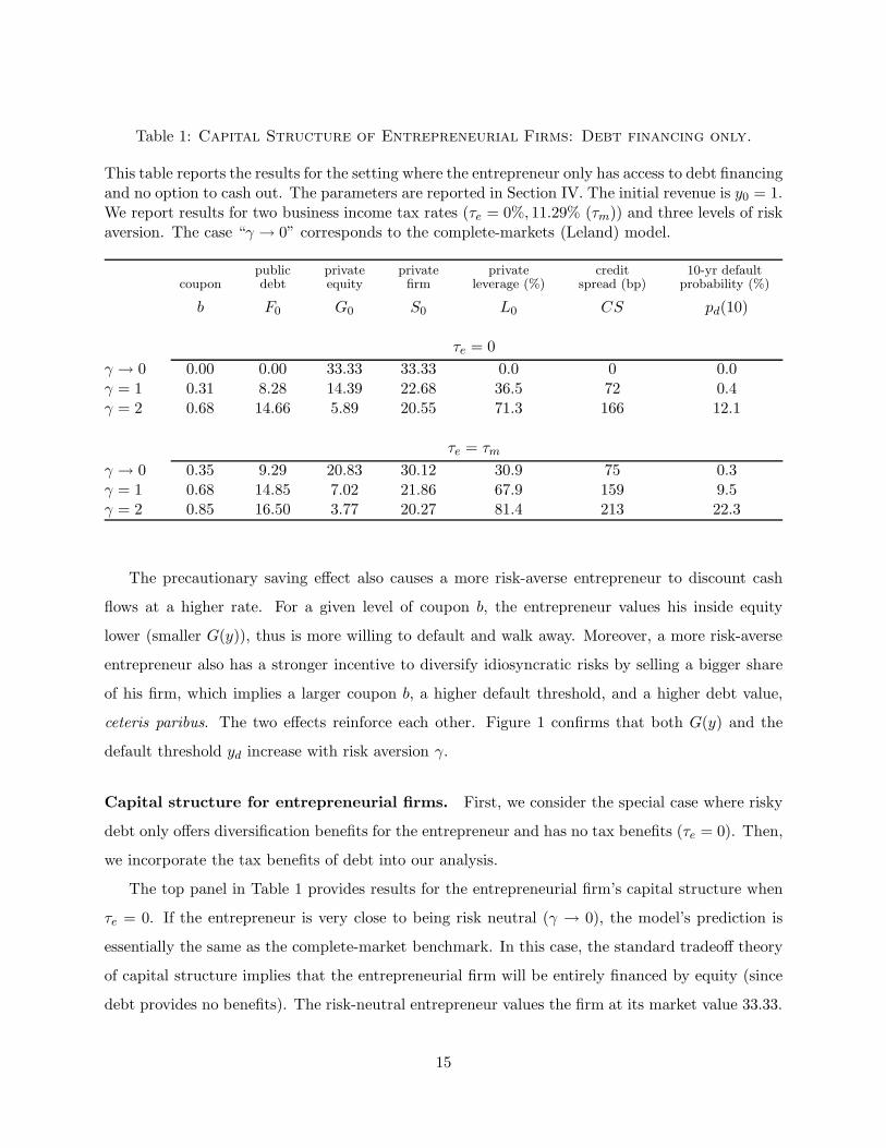
Table 1: Capital Structure of Entrepreneurial Firms: Debt financing only.

This table reports the results for the setting where the entrepreneur only has access to debt financingand no option to cash out. The parameters are reported in Section IV. The initial revenue is y0 = 1.We report results for two business income tax rates (τe = 0%, 11.29% (τm)) and three levels of riskaversion. The case “γ → 0” corresponds to the complete-markets (Leland) model.

public private private private credit 10-yr defaultcoupon debt equity firm leverage (%) spread (bp) probability (%)

b F0 G0 S0 L0 CS pd(10)

τe = 0

γ → 0 0.00 0.00 33.33 33.33 0.0 0 0.0γ = 1 0.31 8.28 14.39 22.68 36.5 72 0.4γ = 2 0.68 14.66 5.89 20.55 71.3 166 12.1

τe = τm

γ → 0 0.35 9.29 20.83 30.12 30.9 75 0.3γ = 1 0.68 14.85 7.02 21.86 67.9 159 9.5γ = 2 0.85 16.50 3.77 20.27 81.4 213 22.3

The precautionary saving effect also causes a more risk-averse entrepreneur to discount cash

flows at a higher rate. For a given level of coupon b, the entrepreneur values his inside equity

lower (smaller G(y)), thus is more willing to default and walk away. Moreover, a more risk-averse

entrepreneur also has a stronger incentive to diversify idiosyncratic risks by selling a bigger share

of his firm, which implies a larger coupon b, a higher default threshold, and a higher debt value,

ceteris paribus. The two effects reinforce each other. Figure 1 confirms that both G(y) and the

default threshold yd increase with risk aversion γ.

Capital structure for entrepreneurial firms. First, we consider the special case where risky

debt only offers diversification benefits for the entrepreneur and has no tax benefits (τe = 0). Then,

we incorporate the tax benefits of debt into our analysis.

The top panel in Table 1 provides results for the entrepreneurial firm’s capital structure when

τe = 0. If the entrepreneur is very close to being risk neutral (γ → 0), the model’s prediction is

essentially the same as the complete-market benchmark. In this case, the standard tradeoff theory

of capital structure implies that the entrepreneurial firm will be entirely financed by equity (since

debt provides no benefits). The risk-neutral entrepreneur values the firm at its market value 33.33.

15

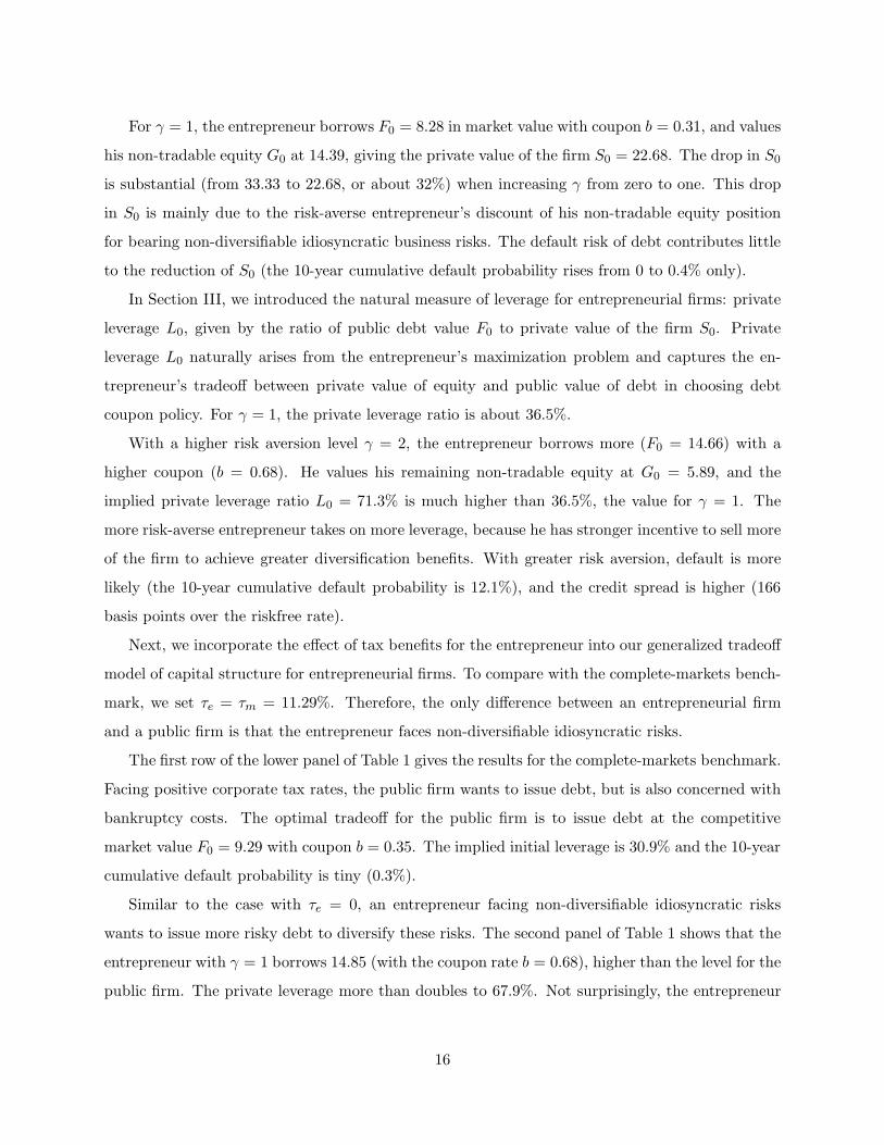
For γ = 1, the entrepreneur borrows F0 = 8.28 in market value with coupon b = 0.31, and values

his non-tradable equity G0 at 14.39, giving the private value of the firm S0 = 22.68. The drop in S0

is substantial (from 33.33 to 22.68, or about 32%) when increasing γ from zero to one. This drop

in S0 is mainly due to the risk-averse entrepreneur’s discount of his non-tradable equity position

for bearing non-diversifiable idiosyncratic business risks. The default risk of debt contributes little

to the reduction of S0 (the 10-year cumulative default probability rises from 0 to 0.4% only).

In Section III, we introduced the natural measure of leverage for entrepreneurial firms: private

leverage L0, given by the ratio of public debt value F0 to private value of the firm S0. Private

leverage L0 naturally arises from the entrepreneur’s maximization problem and captures the en-

trepreneur’s tradeoff between private value of equity and public value of debt in choosing debt

coupon policy. For γ = 1, the private leverage ratio is about 36.5%.

With a higher risk aversion level γ = 2, the entrepreneur borrows more (F0 = 14.66) with a

higher coupon (b = 0.68). He values his remaining non-tradable equity at G0 = 5.89, and the

implied private leverage ratio L0 = 71.3% is much higher than 36.5%, the value for γ = 1. The

more risk-averse entrepreneur takes on more leverage, because he has stronger incentive to sell more

of the firm to achieve greater diversification benefits. With greater risk aversion, default is more

likely (the 10-year cumulative default probability is 12.1%), and the credit spread is higher (166

basis points over the riskfree rate).

Next, we incorporate the effect of tax benefits for the entrepreneur into our generalized tradeoff

model of capital structure for entrepreneurial firms. To compare with the complete-markets bench-

mark, we set τe = τm = 11.29%. Therefore, the only difference between an entrepreneurial firm

and a public firm is that the entrepreneur faces non-diversifiable idiosyncratic risks.

The first row of the lower panel of Table 1 gives the results for the complete-markets benchmark.

Facing positive corporate tax rates, the public firm wants to issue debt, but is also concerned with

bankruptcy costs. The optimal tradeoff for the public firm is to issue debt at the competitive

market value F0 = 9.29 with coupon b = 0.35. The implied initial leverage is 30.9% and the 10-year

cumulative default probability is tiny (0.3%).

Similar to the case with τe = 0, an entrepreneur facing non-diversifiable idiosyncratic risks

wants to issue more risky debt to diversify these risks. The second panel of Table 1 shows that the

entrepreneur with γ = 1 borrows 14.85 (with the coupon rate b = 0.68), higher than the level for the

public firm. The private leverage more than doubles to 67.9%. Not surprisingly, the entrepreneur

16

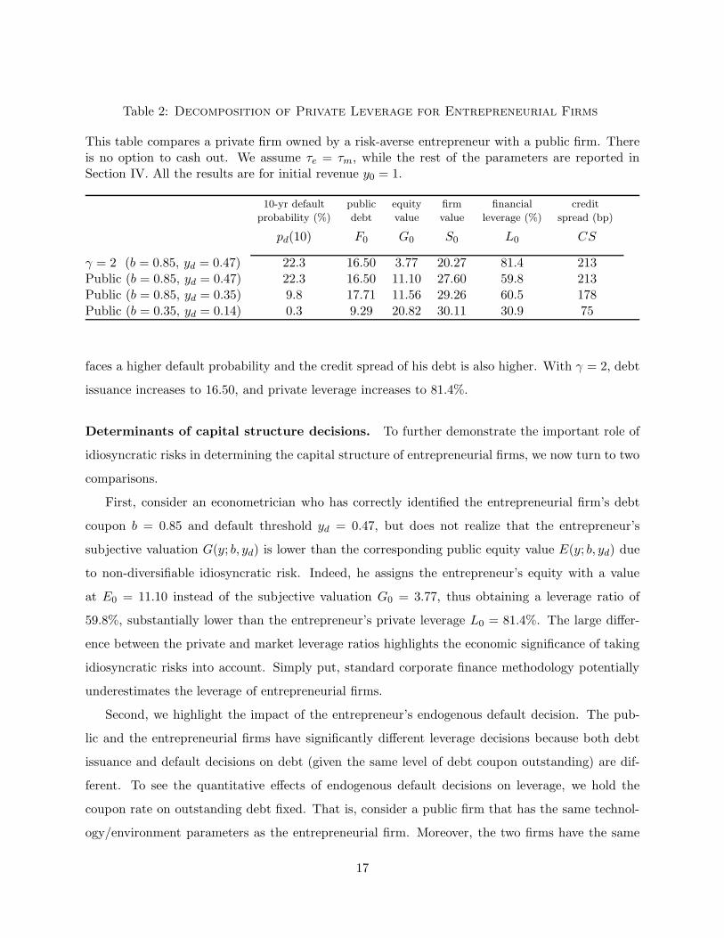
Table 2: Decomposition of Private Leverage for Entrepreneurial Firms

This table compares a private firm owned by a risk-averse entrepreneur with a public firm. Thereis no option to cash out. We assume τe = τm, while the rest of the parameters are reported inSection IV. All the results are for initial revenue y0 = 1.

10-yr default public equity firm financial credit

probability (%) debt value value leverage (%) spread (bp)

pd(10) F0 G0 S0 L0 CS

γ = 2 (b = 0.85, yd = 0.47) 22.3 16.50 3.77 20.27 81.4 213Public (b = 0.85, yd = 0.47) 22.3 16.50 11.10 27.60 59.8 213Public (b = 0.85, yd = 0.35) 9.8 17.71 11.56 29.26 60.5 178Public (b = 0.35, yd = 0.14) 0.3 9.29 20.82 30.11 30.9 75

faces a higher default probability and the credit spread of his debt is also higher. With γ = 2, debt

issuance increases to 16.50, and private leverage increases to 81.4%.

Determinants of capital structure decisions. To further demonstrate the important role of

idiosyncratic risks in determining the capital structure of entrepreneurial firms, we now turn to two

comparisons.

First, consider an econometrician who has correctly identified the entrepreneurial firm’s debt

coupon b = 0.85 and default threshold yd = 0.47, but does not realize that the entrepreneur’s

subjective valuation G(y; b, yd) is lower than the corresponding public equity value E(y; b, yd) due

to non-diversifiable idiosyncratic risk. Indeed, he assigns the entrepreneur’s equity with a value

at E0 = 11.10 instead of the subjective valuation G0 = 3.77, thus obtaining a leverage ratio of

59.8%, substantially lower than the entrepreneur’s private leverage L0 = 81.4%. The large differ-

ence between the private and market leverage ratios highlights the economic significance of taking

idiosyncratic risks into account. Simply put, standard corporate finance methodology potentially

underestimates the leverage of entrepreneurial firms.

Second, we highlight the impact of the entrepreneur’s endogenous default decision. The pub-

lic and the entrepreneurial firms have significantly different leverage decisions because both debt

issuance and default decisions on debt (given the same level of debt coupon outstanding) are dif-

ferent. To see the quantitative effects of endogenous default decisions on leverage, we hold the

coupon rate on outstanding debt fixed. That is, consider a public firm that has the same technol-

ogy/environment parameters as the entrepreneurial firm. Moreover, the two firms have the same

17

debt coupons (b = 0.85).

Facing the same coupon b = 0.85, the public firm defaults when revenue reaches the default

threshold yd = 0.35, which is lower than the threshold yd = 0.47 for the entrepreneurial firm.

Intuitively, facing the same coupon b, the entrepreneurial firm defaults earlier than the public firm

because of the entrepreneur’s aversion to non-diversifiable idiosyncratic risk. The implied shorter

distance-to-default for the entrepreneurial firm translates into a higher 10-year default probability

(22% for the entrepreneurial firm versus 10% for the public firm) and a higher credit spread (213

basis points for the entrepreneurial firm versus 178 basis points for the public firm). Defaulting

optimally for the public firm raises its value from S0 = 27.60 to S0 = 29.26.

The preceding two comparisons help explain the differences in leverage ratios between the en-

trepreneurial firm and the public firm. First, fixing both the coupon and the default threshold, the

entrepreneur’s subjective valuation (due to non-diversifiable risks) has significant impact on the im-

plied leverage ratio. Ignoring subjective valuation substantially underestimates the entrepreneurial

firm’s leverage. Second, facing the same coupon, the entrepreneurial firm defaults earlier than the

public firm, which reduces the value of debt and lowers the leverage ratio, but the quantitative effect

seems small. Third, diversification motives make the entrepreneur issue more debt than the public

firm, which further raises the leverage ratio of the entrepreneurial firm. While the numerical results

are parameter specific, the analysis provides support for our intuition that the entrepreneur’s need

for diversification and subjective valuation discount for bearing non-diversifiable idiosyncratic risks

are key determinants of the private leverage for an entrepreneurial firm.

5 Cash-out option as an alternative channel of diversification

We now turn to a richer and more realistic setting where the entrepreneur can diversify idiosyncratic

risks through both the default and cash-out options. The entrepreneur avoids the downside risk

by defaulting if the firm’s stochastic revenue falls to a sufficiently low level. In addition, when the

firm does well enough, the entrepreneur may want to capitalize on the upside by selling the firm to

diversified investors.

In addition to the baseline parameter values from Section IV, we set the effective capital gains

tax rate from selling the business τg = 10%, reflecting the tax deferral advantage of the tax timing

option.13 We set the initial investment cost for the project I = 10, which is 1/3 of the market

13In Appendix D.1, we investigate the effects of different capital gain taxes.

18

0 0.5 1 1.5 2 2.5 3 3.50

10

20

30

40

50

60

70

80

Revenue y

Private value of equity G(y)

Private value of equityValue of going public

0 0.5 1 1.5 2 2.5 3 3.50

5

10

15

20

25

30

Revenue y

G’(y)

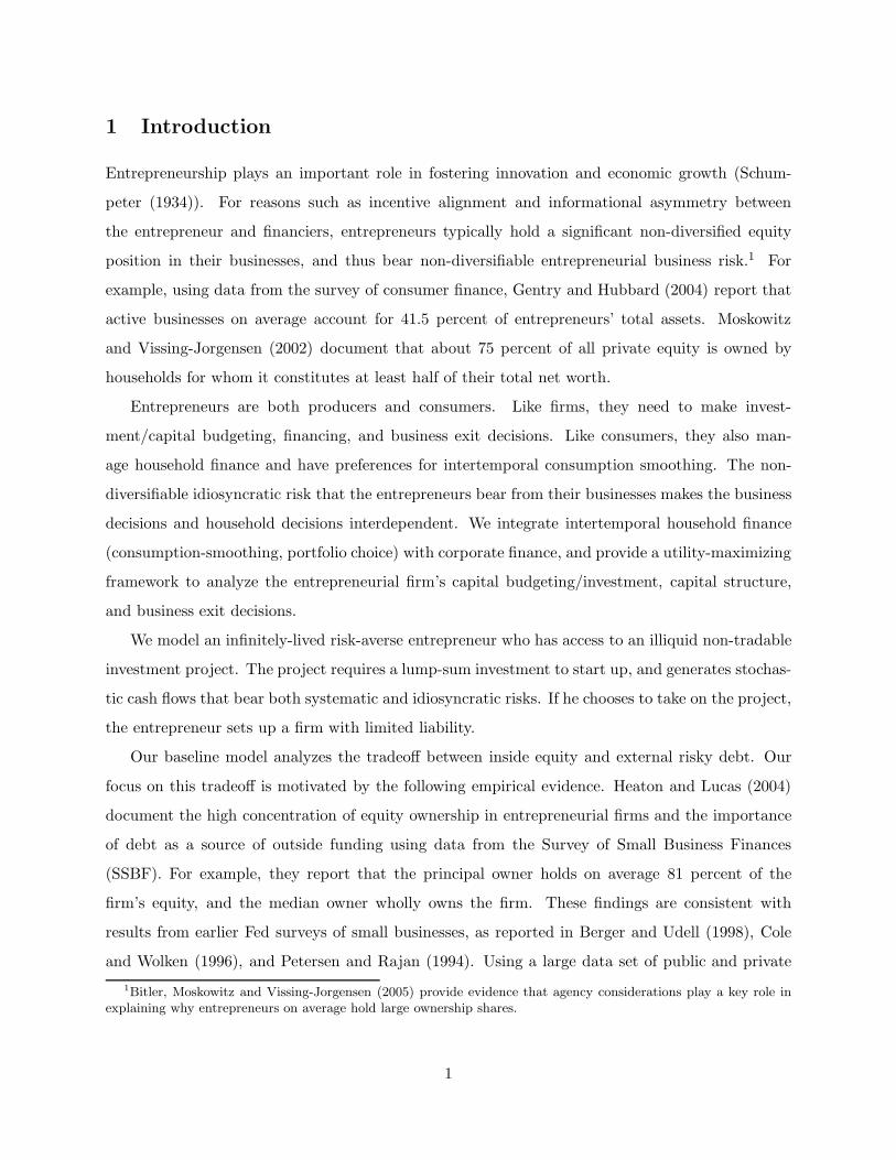
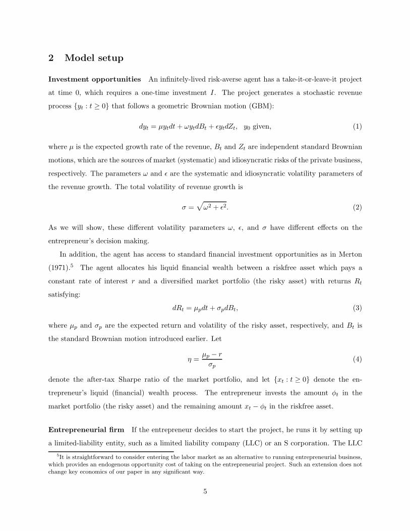
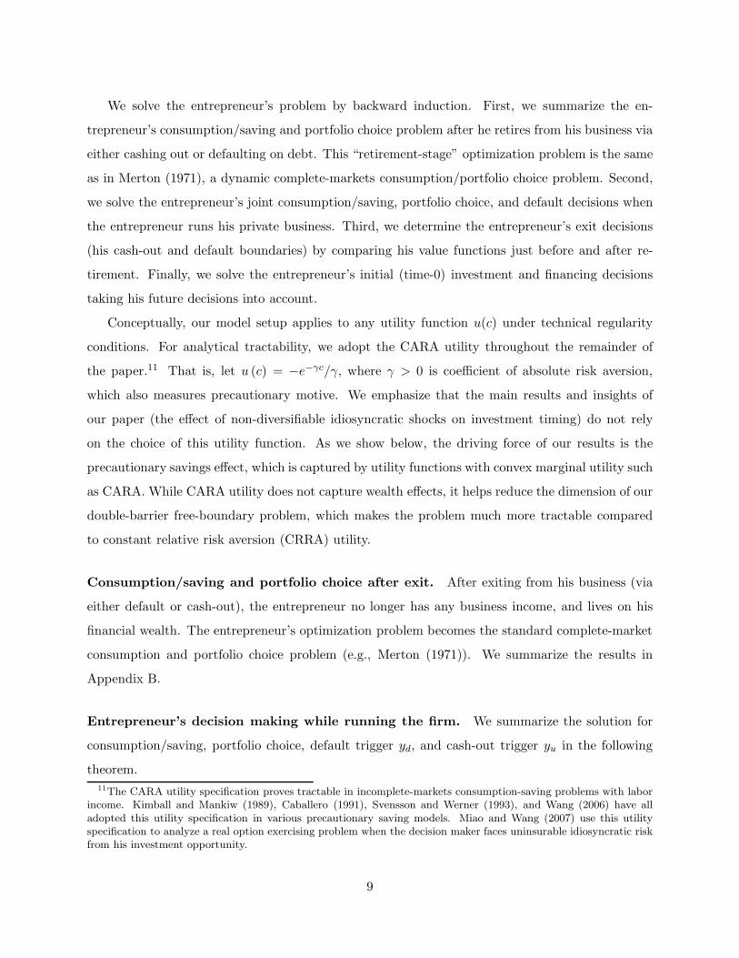
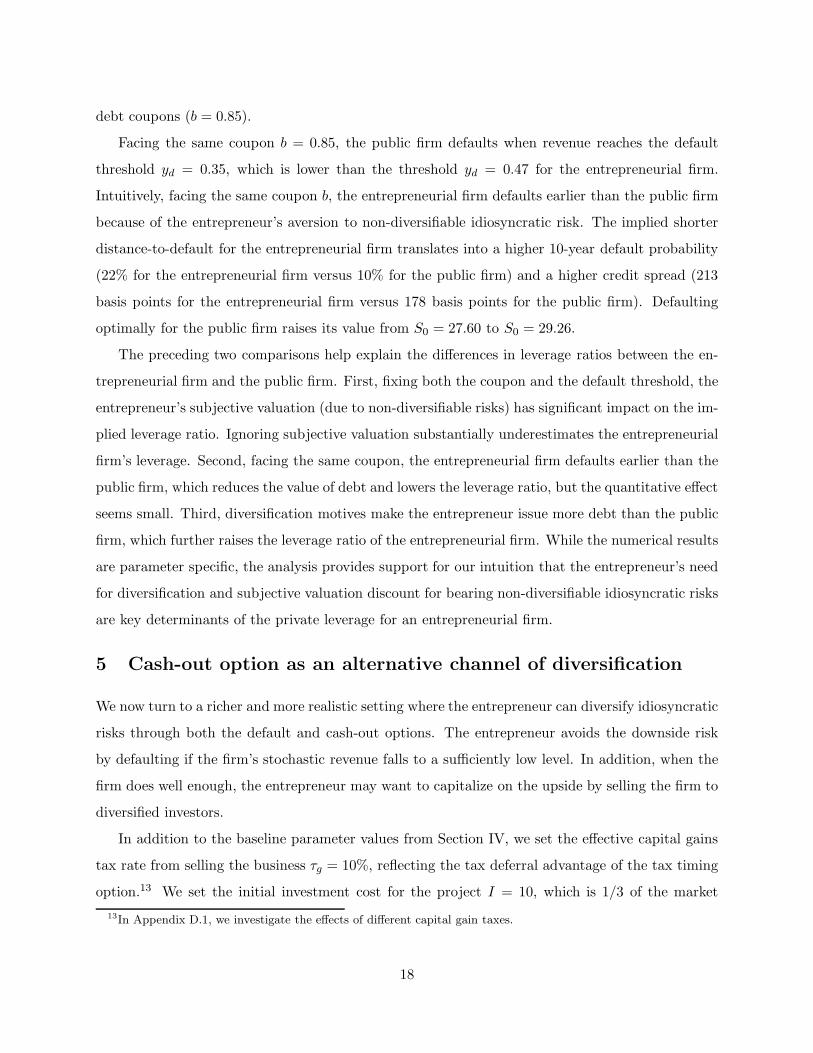
Figure 2: Private value of equity G(y): debt financing and cash-out option. We plot the

results with the following parameters: γ = 1, τe = 0, τg = 10%, I = 10, and K = 27. The remaining

parameters are from the benchmark case reported in Section IV.

value of project cash-flows. We choose the cash-out cost K = 27 to generate a 10-year cash-out

probability of about 20% (with γ = 2), consistent with the success rates of venture capital firms

(Hall and Woodward (2008)).

Cash-out option: Crowding out debt. Figure 2 plots the private value of equity G(y) and

its first derivative G′(y) for an entrepreneur with risk aversion γ = 1 when he has the option to

cash out. The function G (y) smoothly touches the horizontal axis on the left and the dash line

denoting the value of cashing out on the right. The two tangent points give the default and cash-out

thresholds, respectively. For sufficiently low values of revenue y, the private value of equity G(y) is

increasing and convex because the default option is deep in the money. For sufficiently high values

of y, G(y) is also increasing and convex because the cash-out option is deep in the money. For

revenue y in the intermediate range, neither default nor cash-out option is deep in the money. In

this range, the precautionary saving motive may be large enough to induce concavity. As shown in

the right panel of Figure 1, G′ (y) first increases for low values of y, then decreases for intermediate

values of y, and finally increases for high values of y.

Table 3 provides the capital structure information of an entrepreneurial firm with both cash-

out and default options. For brevity, we only report the results for the case τe = τm. When the

market is complete, the firm’s cash-out option is essentially an option to adjust the firm’s capital

19

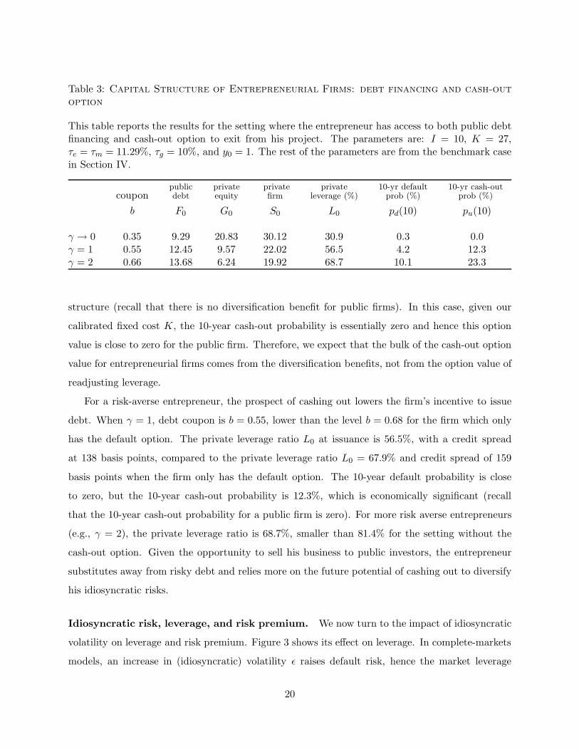
Table 3: Capital Structure of Entrepreneurial Firms: debt financing and cash-outoption

This table reports the results for the setting where the entrepreneur has access to both public debtfinancing and cash-out option to exit from his project. The parameters are: I = 10, K = 27,τe = τm = 11.29%, τg = 10%, and y0 = 1. The rest of the parameters are from the benchmark casein Section IV.

public private private private 10-yr default 10-yr cash-outcoupon debt equity firm leverage (%) prob (%) prob (%)

b F0 G0 S0 L0 pd(10) pu(10)

γ → 0 0.35 9.29 20.83 30.12 30.9 0.3 0.0γ = 1 0.55 12.45 9.57 22.02 56.5 4.2 12.3γ = 2 0.66 13.68 6.24 19.92 68.7 10.1 23.3

structure (recall that there is no diversification benefit for public firms). In this case, given our

calibrated fixed cost K, the 10-year cash-out probability is essentially zero and hence this option

value is close to zero for the public firm. Therefore, we expect that the bulk of the cash-out option

value for entrepreneurial firms comes from the diversification benefits, not from the option value of

readjusting leverage.

For a risk-averse entrepreneur, the prospect of cashing out lowers the firm’s incentive to issue

debt. When γ = 1, debt coupon is b = 0.55, lower than the level b = 0.68 for the firm which only

has the default option. The private leverage ratio L0 at issuance is 56.5%, with a credit spread

at 138 basis points, compared to the private leverage ratio L0 = 67.9% and credit spread of 159

basis points when the firm only has the default option. The 10-year default probability is close

to zero, but the 10-year cash-out probability is 12.3%, which is economically significant (recall

that the 10-year cash-out probability for a public firm is zero). For more risk averse entrepreneurs

(e.g., γ = 2), the private leverage ratio is 68.7%, smaller than 81.4% for the setting without the

cash-out option. Given the opportunity to sell his business to public investors, the entrepreneur

substitutes away from risky debt and relies more on the future potential of cashing out to diversify

his idiosyncratic risks.

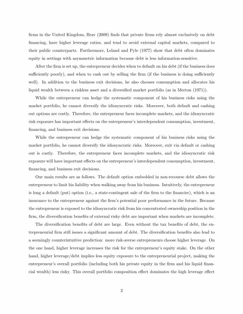
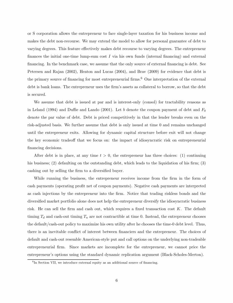
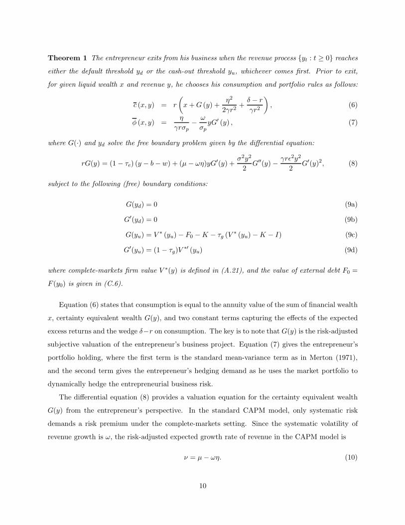
Idiosyncratic risk, leverage, and risk premium. We now turn to the impact of idiosyncratic

volatility on leverage and risk premium. Figure 3 shows its effect on leverage. In complete-markets

models, an increase in (idiosyncratic) volatility ǫ raises default risk, hence the market leverage

20

0 0.05 0.1 0.15 0.2 0.25 0.30.3

0.4

0.5

0.6

0.7

0.8

0.9

Idiosyncratc volatility ε

Coupon b

0 0.05 0.1 0.15 0.2 0.25 0.30.2

0.25

0.3

0.35

0.4

0.45

0.5

0.55

0.6

0.65

0.7

Private leverage L0

Idiosyncratc volatility ε

γ → 0

γ = 0.5

γ = 1

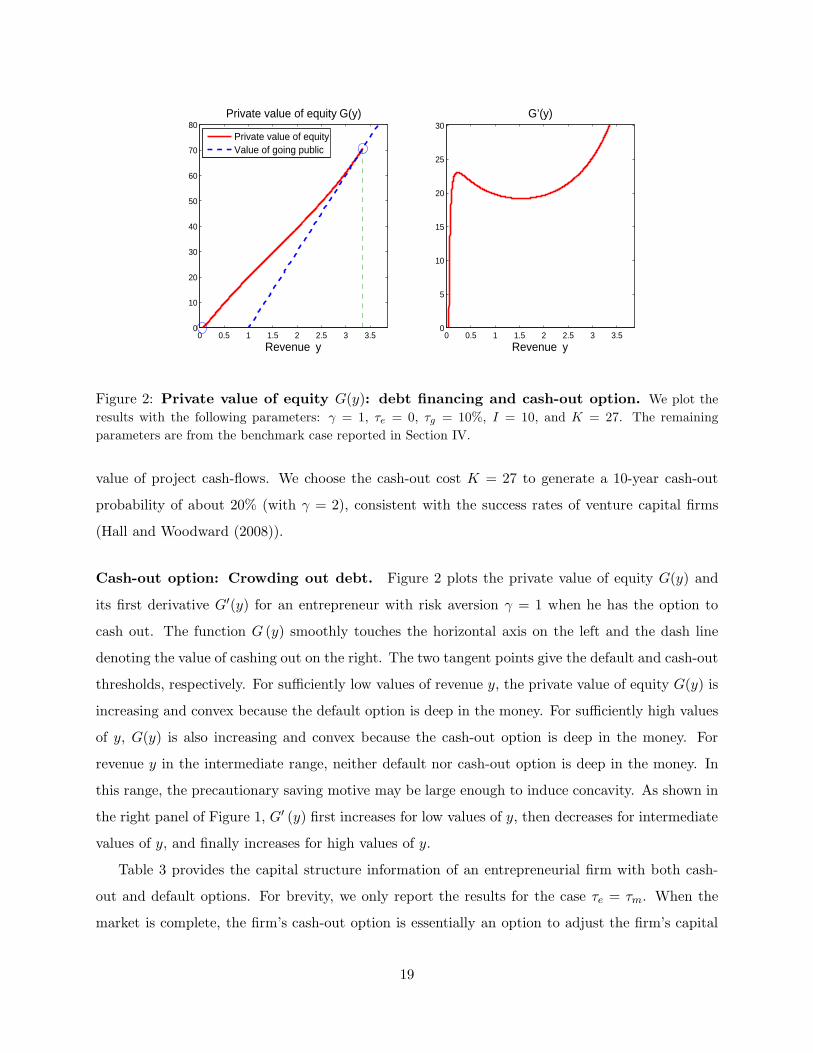
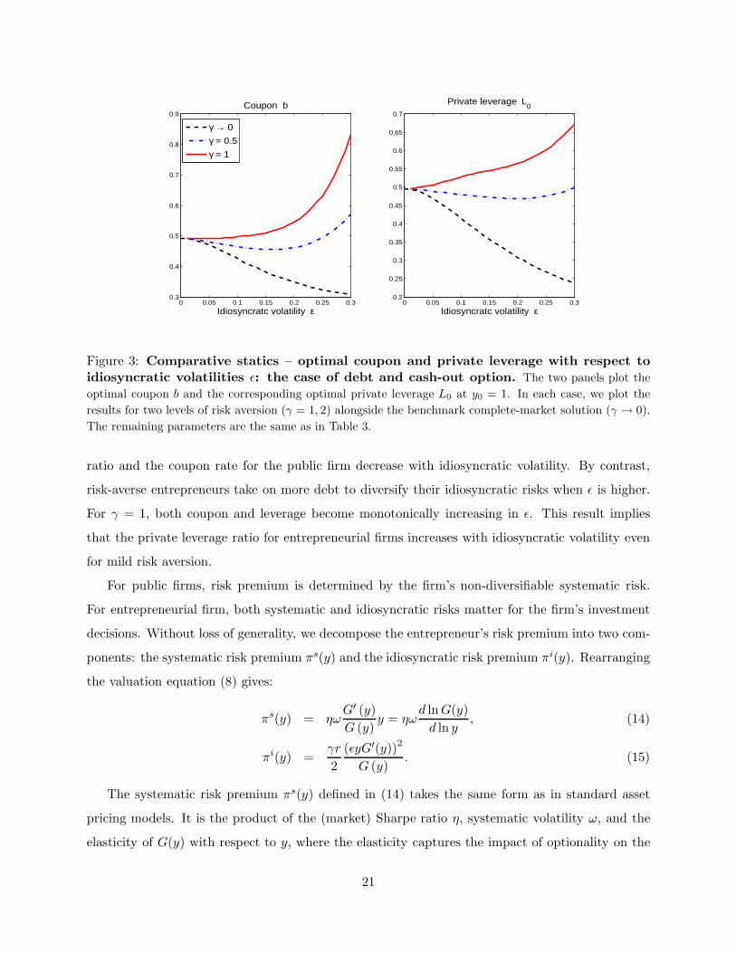
Figure 3: Comparative statics – optimal coupon and private leverage with respect toidiosyncratic volatilities ǫ: the case of debt and cash-out option. The two panels plot the

optimal coupon b and the corresponding optimal private leverage L0 at y0 = 1. In each case, we plot the

results for two levels of risk aversion (γ = 1, 2) alongside the benchmark complete-market solution (γ → 0).

The remaining parameters are the same as in Table 3.

ratio and the coupon rate for the public firm decrease with idiosyncratic volatility. By contrast,

risk-averse entrepreneurs take on more debt to diversify their idiosyncratic risks when ǫ is higher.

For γ = 1, both coupon and leverage become monotonically increasing in ǫ. This result implies

that the private leverage ratio for entrepreneurial firms increases with idiosyncratic volatility even

for mild risk aversion.

For public firms, risk premium is determined by the firm’s non-diversifiable systematic risk.

For entrepreneurial firm, both systematic and idiosyncratic risks matter for the firm’s investment

decisions. Without loss of generality, we decompose the entrepreneur’s risk premium into two com-

ponents: the systematic risk premium πs(y) and the idiosyncratic risk premium πi(y). Rearranging

the valuation equation (8) gives:

πs(y) = ηωG′ (y)

G (y)y = ηω

d lnG(y)

d ln y, (14)

πi(y) =γr

2

(ǫyG′(y))2

G (y). (15)

The systematic risk premium πs(y) defined in (14) takes the same form as in standard asset

pricing models. It is the product of the (market) Sharpe ratio η, systematic volatility ω, and the

elasticity of G(y) with respect to y, where the elasticity captures the impact of optionality on the

21

0 1 2 30

0.1

0.2

0.3

0.4Systematic risk premium πs(y)

Revenue y

γ = 4γ = 2

0 1 2 30

0.1

0.2

0.3

0.4Idiosyncratic risk premium πi(y)

Revenue y

γ = 4γ = 2

0 1 2 30

0.1

0.2

0.3

0.4Systematic risk premium πs(y)

Revenue y

ε = .25ε = .20

0 1 2 30

0.1

0.2

0.3

0.4Idiosyncratic risk premium πi(y)

Revenue y

ε = .25ε = .20

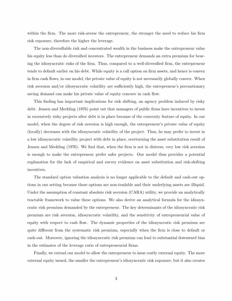
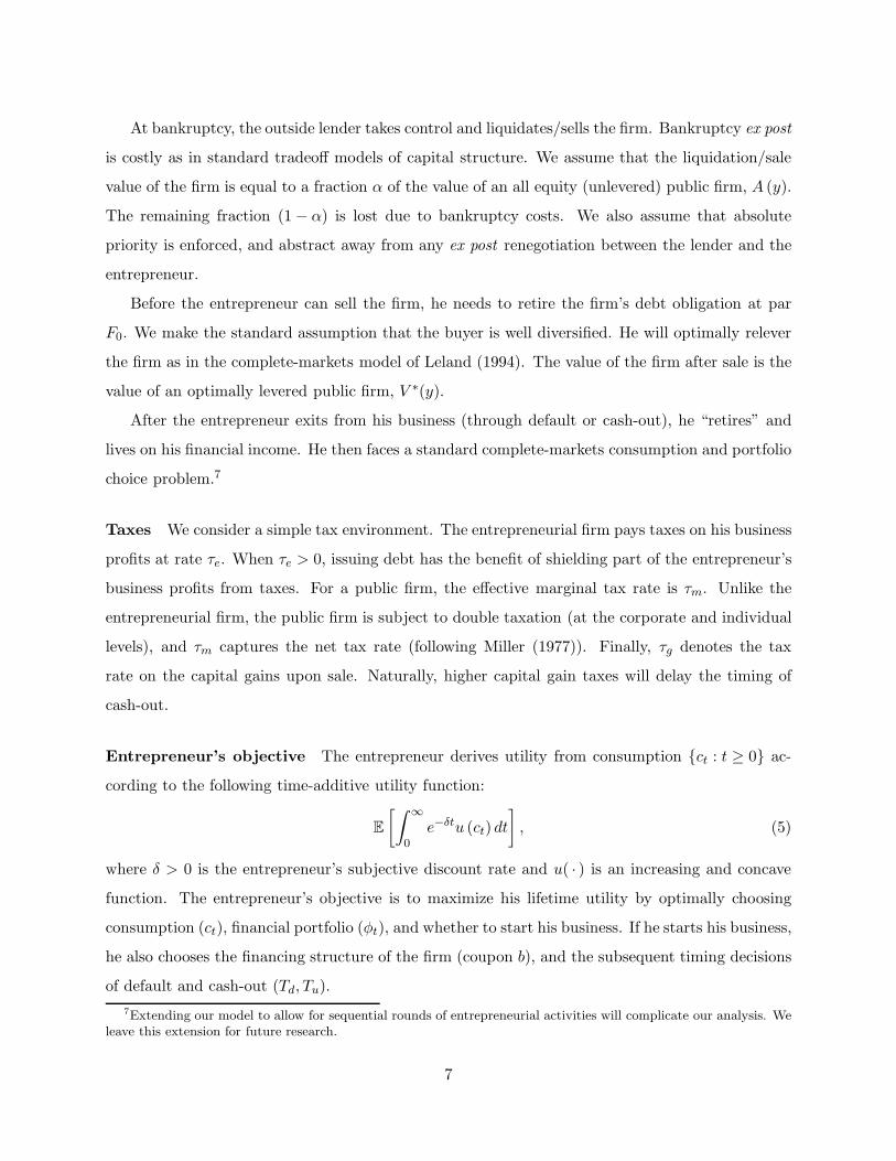
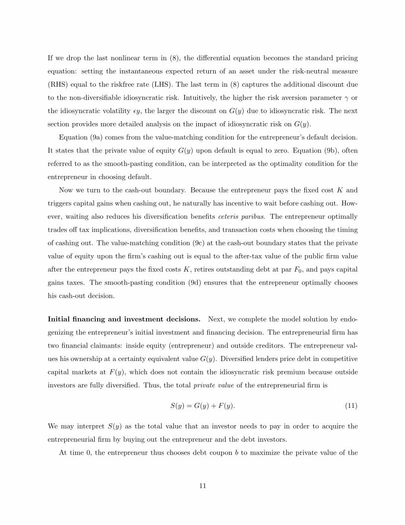
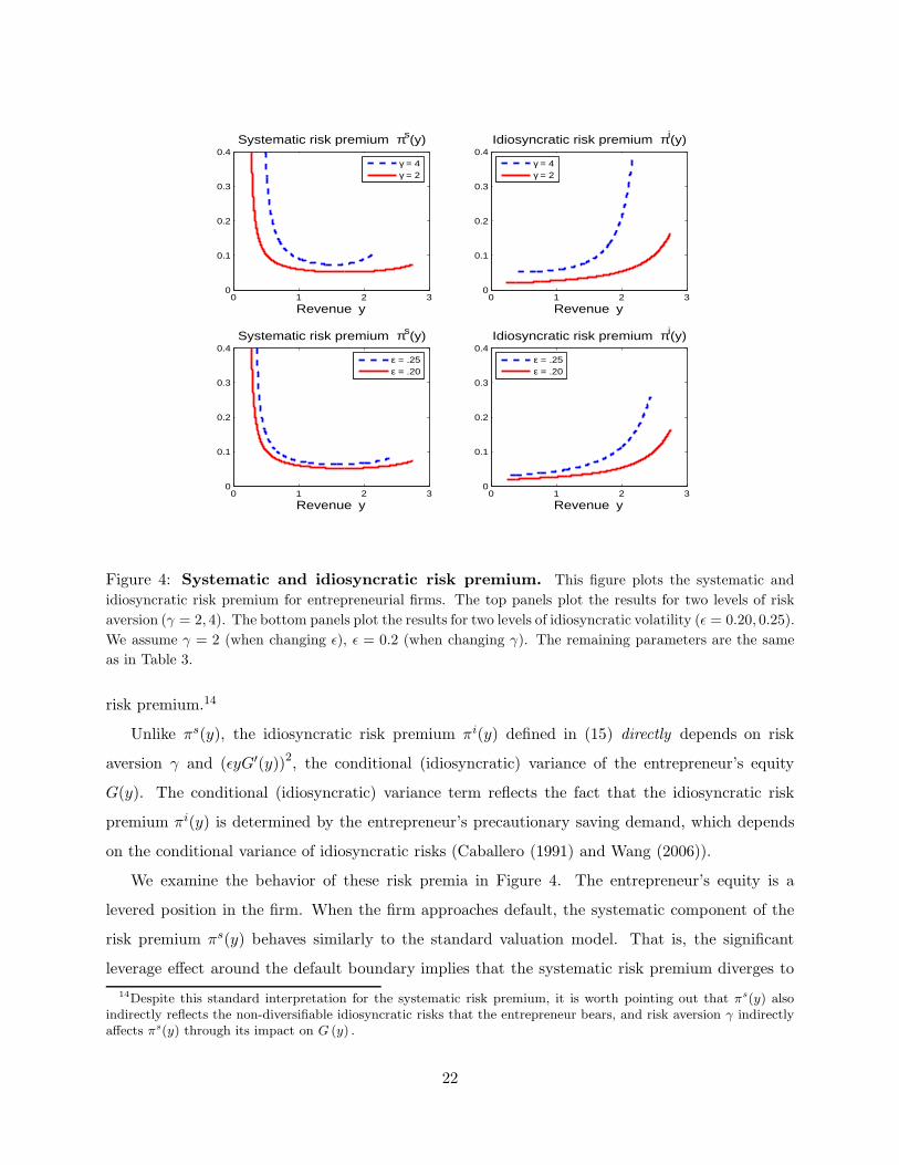
Figure 4: Systematic and idiosyncratic risk premium. This figure plots the systematic and

idiosyncratic risk premium for entrepreneurial firms. The top panels plot the results for two levels of risk

aversion (γ = 2, 4). The bottom panels plot the results for two levels of idiosyncratic volatility (ǫ = 0.20, 0.25).

We assume γ = 2 (when changing ǫ), ǫ = 0.2 (when changing γ). The remaining parameters are the same

as in Table 3.

risk premium.14

Unlike πs(y), the idiosyncratic risk premium πi(y) defined in (15) directly depends on risk

aversion γ and (ǫyG′(y))2, the conditional (idiosyncratic) variance of the entrepreneur’s equity

G(y). The conditional (idiosyncratic) variance term reflects the fact that the idiosyncratic risk

premium πi(y) is determined by the entrepreneur’s precautionary saving demand, which depends

on the conditional variance of idiosyncratic risks (Caballero (1991) and Wang (2006)).

We examine the behavior of these risk premia in Figure 4. The entrepreneur’s equity is a

levered position in the firm. When the firm approaches default, the systematic component of the

risk premium πs(y) behaves similarly to the standard valuation model. That is, the significant

leverage effect around the default boundary implies that the systematic risk premium diverges to

14Despite this standard interpretation for the systematic risk premium, it is worth pointing out that πs(y) alsoindirectly reflects the non-diversifiable idiosyncratic risks that the entrepreneur bears, and risk aversion γ indirectlyaffects πs(y) through its impact on G (y) .

22

infinity when y approaches yd. When the firm approaches the cash-out threshold, the cash-out

option makes the firm value more sensitive to cash flow shocks, which also tends to raise the

systematic risk premium.

The idiosyncratic risk premium πi(y) behaves quite differently. Figure 4 indicates that the

idiosyncratic risk premium is small when the firm is close to default, and it increases with y for most

values of y. The intuition is as follows. The numerator in (15) reflects the agent’s precautionary

saving demand, which depends on the conditional idiosyncratic variance of the changes in the

certainty equivalent value of equity G(y) and risk aversion γ. Both the conditional idiosyncratic

variance and G(y) increase with y. When y is large, the conditional idiosyncratic variance rises fast

relative to G(y), generating a large idiosyncratic risk premium.

6 Project choice: asset substitution versus risk sharing

Jensen and Meckling (1976) point out that there is an incentive problem associated with risky

debt: After debt is in place, managers have incentive to take on riskier projects to take advantage

of the option-type of payoff structure of equity. However, there is little empirical evidence in

support of such risk shifting behaviors.15 One possible explanation is that managerial risk aversion

can potentially dominate the risk shifting incentives. Our model provides a natural setting to

investigate these two competing effects quantitatively.

We consider the following project choice problem. Suppose the risk-averse entrepreneur can

choose among a continuum of mutually exclusive projects with different idiosyncratic volatilities ǫ

in the interval [ǫmin, ǫmax] after debt is in place. Let F0 be the market value of existing debt with

the coupon payment b. The entrepreneur then chooses idiosyncratic volatility ǫ+ ∈ [ǫmin, ǫmax]

to maximize his own utility. As shown in Section III, the entrepreneur effectively chooses ǫ+ to

maximize his private value of equity G(y0), taking the debt contract (b, F0) as given. Let this

maximized value be G+ (y0).

In a rational expectations equilibrium, the lender anticipates the entrepreneur’s ex post incentive

of choosing the level of idiosyncratic volatility ǫ+ to maximize G(y0), and prices the initial debt

contract accordingly in competitive capital markets. Therefore, the entrepreneur ex ante maximizes

the private value of the firm, S(y0) = G+(y0)+F0, taking the competitive market debt pricing into

account. We solve this joint investment and financing (fixed-point) problem.

15See Andrade and Kaplan (1998), Graham and Harvey (2001), and Rauh (2008), among others.

23

0.05 0.1 0.15 0.2 0.25 0.3 0.358

10

12

14

16

18

20

22

24

Idiosyncratc volatility ε

Private value of equity G(y0)

γ → 0: ε+ = 0.35, b* = 0.297

γ = 0.1: ε+ = 0.05, b* = 0.472

γ = 1.0: ε+ = 0.05, b* = 0.491

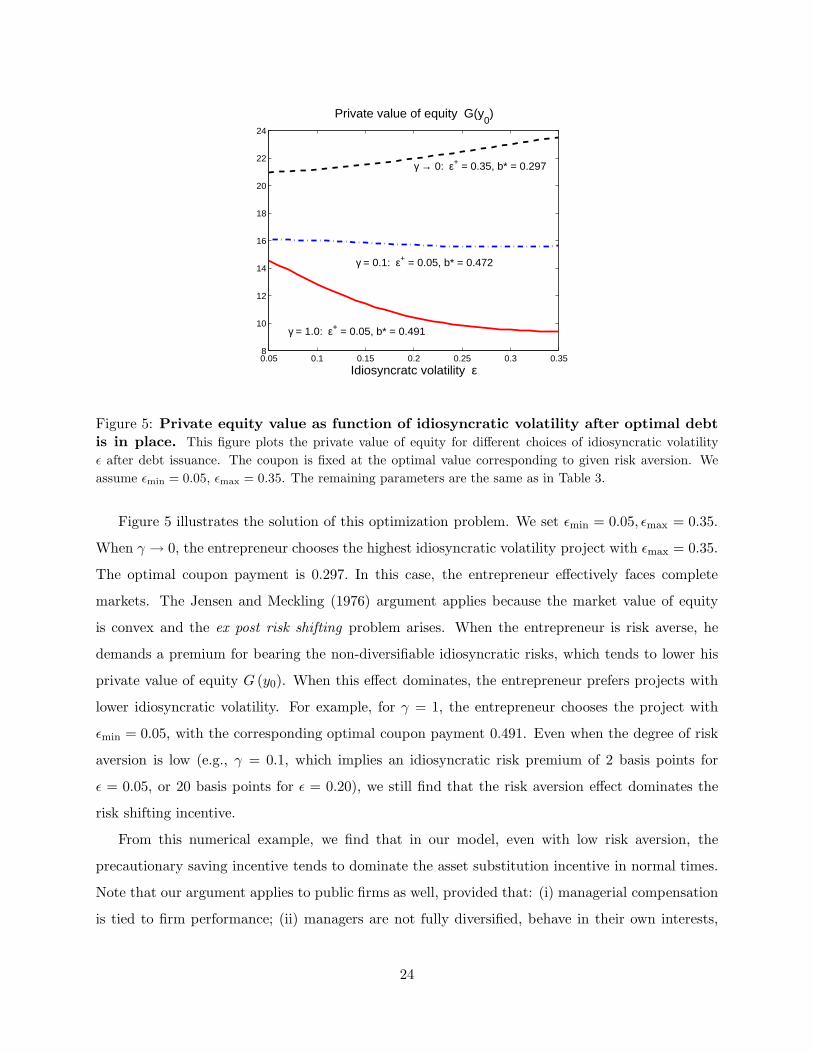
Figure 5: Private equity value as function of idiosyncratic volatility after optimal debtis in place. This figure plots the private value of equity for different choices of idiosyncratic volatility

ǫ after debt issuance. The coupon is fixed at the optimal value corresponding to given risk aversion. We

assume ǫmin = 0.05, ǫmax = 0.35. The remaining parameters are the same as in Table 3.

Figure 5 illustrates the solution of this optimization problem. We set ǫmin = 0.05, ǫmax = 0.35.

When γ → 0, the entrepreneur chooses the highest idiosyncratic volatility project with ǫmax = 0.35.

The optimal coupon payment is 0.297. In this case, the entrepreneur effectively faces complete

markets. The Jensen and Meckling (1976) argument applies because the market value of equity

is convex and the ex post risk shifting problem arises. When the entrepreneur is risk averse, he

demands a premium for bearing the non-diversifiable idiosyncratic risks, which tends to lower his

private value of equity G (y0). When this effect dominates, the entrepreneur prefers projects with

lower idiosyncratic volatility. For example, for γ = 1, the entrepreneur chooses the project with

ǫmin = 0.05, with the corresponding optimal coupon payment 0.491. Even when the degree of risk

aversion is low (e.g., γ = 0.1, which implies an idiosyncratic risk premium of 2 basis points for

ǫ = 0.05, or 20 basis points for ǫ = 0.20), we still find that the risk aversion effect dominates the

risk shifting incentive.

From this numerical example, we find that in our model, even with low risk aversion, the

precautionary saving incentive tends to dominate the asset substitution incentive in normal times.

Note that our argument applies to public firms as well, provided that: (i) managerial compensation

is tied to firm performance; (ii) managers are not fully diversified, behave in their own interests,

24

and are entrenched. Thus, the lack of empirical evidence supporting asset substitution may be

simply due to the non-diversifiable idiosyncratic risks faced by risk-averse decision makers.

7 External equity

While debt is the primary source of financing for most entrepreneurial (small-business) firms, high-

tech startups are often financed by venture capital, which often use external equity in various forms

as the primary source of financing. This financing choice particularly makes sense when the liquida-

tion value of firm’s assets is low (e.g., computer software firms), and incentive alignments are more

important. Hall and Woodward (2008) provide a quantitative analysis for the lack of diversification

of venture-capital-backed entrepreneurial firms. In this section, we extend the baseline model of

Section II by allowing the entrepreneur to issue external equity at t = 0, and study the effect of

external equity on the diversification benefits of risky debt.16

If it is costless to issue external equity, a risk-averse entrepreneur will want to sell the entire

firm to the VC right away. We motivate the costs of external equity through the agency problems

of Jensen and Meckling (1976). Intuitively, the more concentrated the entrepreneur’s ownership is,

the better incentive alignment (Berle and Means (1931) and Jensen and Meckling (1976)). Let ψ

denote the fraction of equity that the entrepreneur retains and hence 1 − ψ denote the fraction of

external equity. Consider the expected growth rate of revenue µ in equation (1). We capture the

incentive problem of ownership in reduced form by making µ an increasing and concave function

of the entrepreneur’s ownership ψ (i.e., µ′(ψ) > 0 and µ′′(ψ) < 0). Intuitively, the concavity

relation suggests that the incremental value from incentive alignment becomes lower as ownership

concentration rises, ceteris paribus.

More specifically, we model the growth rate µ as a quadratic function of the entrepreneur’s

ownership ψ, µ(ψ) = −0.02ψ2 + 0.04ψ + 0.03, with ψ ∈ [0, 1]. This functional form is chosen such

that the maximum expected growth rate is 5%, when the entrepreneur owns the entire firm (ψ = 1),

while the lowest growth rate is 3%, when the entire firm is sold (ψ = 0). The parameters for µ(ψ)

are chosen to keep the agency costs of external equity modest so as to highlight the substitution

effect of external equity.

After external debt (with coupon b) and equity (with share 1 − ψ of the firm ownership) are

16Initial equity issuance together with cashing out can be viewed as a two-step procedure to unload the en-trepreneur’s private holdings. Gradual sales of ownership, e.g., as DeMarzo and Urosevic (2006) consider for largeshareholders, is less applicable for private business owners due to the lack of liquidity, which we capture with thefixed cost K.

25

issued at t = 0, the entrepreneur’s optimal policies, including consumption/portfolio rule and

default/cash-out policies, are summarized in the following theorem.

Theorem 2 The entrepreneur exits from his business when the revenue process {yt : t ≥ 0} reaches

either the default threshold yd or the cash-out threshold yu, whichever occurs first. When the

entrepreneur runs his firm, he chooses his consumption and portfolio rules as follows:

c (x, y) = r

(

x+ ψG (y) +η2

2γr2+δ − r

γr2

)

, (16)

φ (x, y) =η

γrσp−ψω

σpyG′ (y) , (17)

where (G( · ), yd, yu) solves the free boundary problem given by the differential equation:

rG(y) = (1 − τe) (y − b− w) + νyG′(y) +σ2y2

2G′′(y) −

ψγrǫ2y2

2G′(y)2, (18)

subject to the following (free) boundary conditions:

G(yd) = 0 (19a)

G′(yd) = 0 (19b)

ψG(yu) = ψV ∗ (yu) − F0 −K − τg (ψV ∗ (yu) −K − (I − (1 − ψ)E0)) (19c)

ψG′(yu) = (1 − τg)ψV∗′ (yu) (19d)

where complete-markets firm value V ∗(y) is defined in (A.21), the value of external debt F0 = F (y0)

is given in (C.6), and the value of external equity E0 = E(y0) is given by (C.10).

Equation (18) shows how the partial ownership ψ affects the entrepreneur’s private value of

equity. A more concentrated inside equity position (higher ψ) raises the last nonlinear term, which

raises the idiosyncratic risk premium that the entrepreneur demands. The ownership ψ also affects

the boundary conditions at cash-out. The value-matching condition (19c) at the cash-out boundary

states that, upon cashing out, the entrepreneur’s ownership is worth fraction ψ of the after-tax value

of the public firm value net of (1) the amount required to retire outstanding debt at par F0, (2)

fixed costs K, and (3) capital gains taxes. The smooth-pasting condition (19d) also reflects the

effects of partial ownership.

Finally, at time t = 0, the entrepreneur chooses debt coupon b and initial ownership ψ to

maximize the private value of the firm S(y), which now has three parts: inside equity (entrepreneur’s

ownership), diversified outside equity, and outside debt:

S(y) = ψG(y) + (1 − ψ)E0(y) + F (y). (20)

26

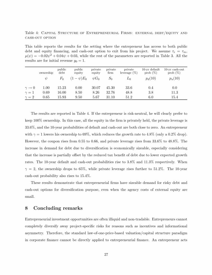
Table 4: Capital Structure of Entrepreneurial Firms: external debt/equity andcash-out option

This table reports the results for the setting where the entrepreneur has access to both publicdebt and equity financing, and cash-out option to exit from his project. We assume τe = τm,µ(ψ) = −0.02ψ2 + 0.04ψ + 0.03, while the rest of the parameters are reported in Table 3. All theresults are for initial revenue y0 = 1.

public public private private private 10-yr default 10-yr cash-outownership debt equity equity firm leverage (%) prob (%) prob (%)

ψ F0 (1 − ψ)E0 ψG0 S0 L0 pd(10) pu(10)

γ → 0 1.00 15.23 0.00 30.07 45.30 33.6 0.4 0.0γ = 1 0.69 16.00 8.50 8.26 32.76 48.8 3.8 11.3γ = 2 0.65 15.93 9.50 5.67 31.10 51.2 6.0 15.4

The results are reported in Table 4. If the entrepreneur is risk-neutral, he will clearly prefer to

keep 100% ownership. In this case, all the equity in the firm is privately held, the private leverage is

33.6%, and the 10-year probabilities of default and cash-out are both close to zero. An entrepreneur

with γ = 1 lowers his ownership to 69%, which reduces the growth rate to 4.8% (only a 0.2% drop).

However, the coupon rises from 0.55 to 0.66, and private leverage rises from 33.6% to 48.8%. The

increase in demand for debt due to diversification is economically sizeable, especially considering

that the increase is partially offset by the reduced tax benefit of debt due to lower expected growth

rates. The 10-year default and cash-out probabilities rise to 3.8% and 11.3% respectively. When

γ = 2, the ownership drops to 65%, while private leverage rises further to 51.2%. The 10-year

cash-out probability also rises to 15.4%.

These results demonstrate that entrepreneurial firms have sizeable demand for risky debt and

cash-out options for diversification purpose, even when the agency costs of external equity are

small.

8 Concluding remarks

Entrepreneurial investment opportunities are often illiquid and non-tradable. Entrepreneurs cannot

completely diversify away project-specific risks for reasons such as incentives and informational

asymmetry. Therefore, the standard law-of-one-price-based valuation/capital structure paradigm

in corporate finance cannot be directly applied to entrepreneurial finance. An entrepreneur acts

27

both as a producer making dynamic investment, financing, and exit decisions for his business

project, and as a household making consumption/saving and portfolio decisions. The dual roles of

the entrepreneur motivate us to develop a dynamic incomplete-markets model of entrepreneurial

finance that centers around the non-diversification feature of the entrepreneurial business.

We show that more risk-averse entrepreneurs use higher leverage for greater diversification ben-

efits and default earlier. This prediction holds not only in the baseline setting where the source

of external financing is risky debt, but is robust when we introduce additional channels of diver-

sification such as cash-out option and external equity. In addition to compensation for systematic

risks, the entrepreneur also demands sizable premium for bearing idiosyncratic risks, which increase

with his risk aversion, his equilibrium inside ownership, and the project’s idiosyncratic variance.

Ignoring this idiosyncratic risk premium can lead to a large upward bias when computing the pri-

vate value of entrepreneurial equity. Finally, even for low to moderate levels of risk aversion, the

idiosyncratic risk premium significantly weakens the risk shifting incentives (Jensen and Meckling

(1976)) for non-diversified managers.

Our paper also makes methodological contributions to financial valuation and decision making.

This paper extends the standard complete-markets Black-Scholes-Merton option pricing and real

options methodology to settings where investment opportunities are illiquid and not marked-to-

market, and decision makers are not diversified. Our framework can also be used to value the stock

options of non-diversified executives or to analyze how these executives make capital structure and

investment decisions. See Carpenter, Stanton, and Wallace (2008) for a recent study on the optimal

exercise policy for an executive stock option and implications for firm costs.

We have taken a standard optimization framework where the entrepreneur’s utility only depends

on his consumption. A significant fraction of entrepreneurs view the non-pecuniary benefits of

being their own bosses as a large component of rewards. It has also been documented that less

risk-averse (see Gentry and Hubbard (2004), De Nardi, Doctor, and Krane (2007)) and more

confident/optimistic individuals are more likely to self-select into entrepreneurship. We also do

not model the fundamental frictions causing markets to be incomplete and entrepreneurs to be

non-diversified. We view endogenous incomplete markets as a complementary perspective, which

can have fundamental implications such as promotion of entrepreneurship and contract design. We

leave these extensions for future research.

28

Appendix

A Market valuation and capital structure of a public firm

Well-diversified owners of a public firm face complete markets. Given the Sharpe ratio η of the

market portfolio and the riskfree rate r, there exists a unique stochastic discount factor (SDF)

(ξt : t ≥ 0) satisfying (see Duffie (2001)):

dξt = −rξtdt− ηξtdBt, ξ0 = 1. (A.1)

Using this SDF, we can derive the market value of the unlevered firm, A (y) , the market value of

equity, E (y) , and the market value of debt D (y) . The market value of the firm is equal to the

sum of equity value and debt value:

V (y) = E (y) +D (y) . (A.2)

Under the risk-neutral probability measure Q, we can rewrite the dynamics of the revenue (1)

as follows:

dyt = νytdt + ωytdBQt + ǫytdZt, (A.3)

where ν is the risk-adjusted drift defined by ν ≡ µ − ωη, and BQt is a standard Brownian motion

under Q satisfying dBQt = dBt + ηdt.

A.1 Valuation of an unlevered public firm

Throughout the appendix, we derive our results assuming that there is a flow operating cost w for

running the project. The operating cost w generates operating leverage and hence the option to

abandon the firm has positive value. The results reported in this paper are for the case w = 0.

Appendix D.2 provides results for the case w > 0.

We start with the after-tax unlevered firm value A (y), which satisfies the following differential

equation:

rA (y) = (1 − τm) (y −w) + νyA′ (y) +1

2σ2y2A′′ (y) . (A.4)

This is a second-order ordinary differential equation (ODE). We need two boundary conditions to

obtain a solution. One boundary condition describes the behavior of A (y) when y → ∞. This

condition rules out speculative bubbles. To ensure that A (y) is finite, we assume r > ν throughout

the paper. The other boundary condition is related to abandonment. As in the standard option

29

exercise models, the firm is abandoned whenever the cash flow process hits a threshold value ya for

the first time. At the threshold ya, the following value-matching condition is satisfied

A (ya) = 0, (A.5)

because we normalize the outside value to zero. For the abandonment threshold ya to be optimal,

the following smooth-pasting condition must also be satisfied:

A′ (ya) = 0. (A.6)

Solving equation (A.4) and using the no-bubble condition and boundary conditions (A.5)-(A.6), we

obtain

A (y) = (1 − τm)

[

(

y

r − ν−w

r

)

−

(

yar − ν

−w

r

)(

y

ya

)θ1]

, (A.7)

where the abandonment threshold ya is given in

ya =r − ν

r

θ1θ1 − 1

w, (A.8)

where

θ1 = −σ−2(

ν − σ2/2)

−

√

σ−4 (ν − σ2/2)2 + 2rσ−2 < 0. (A.9)

A.2 Valuation of a levered public firm

First, consider the market value of equity. Let yd be the corresponding default threshold. After

default, equity is worthless, in that E(y) = 0 for y ≤ yd. This gives us the value matching condition

E (yd) = 0. Before default, equity value E (y) satisfies the following differential equation:

rE (y) = (1 − τm) (y −w − b) + νyE′ (y) +1

2σ2y2E′′ (y) , y ≥ yd. (A.10)

When y → ∞, E (y) also satisfies a no-bubble condition. Solving this ODE and using the boundary

conditions, we obtain

E (y; yd) = (1 − τm)

[

(

y

r − ν−w + b

r

)

−

(

ydr − ν

−w + b

r

)(

y

yd

)θ1]

. (A.11)

Equation (A.11) shows that equity value is equal to the after-tax present value of profit flows

minus the present value of the perpetual coupon payments plus an option value to default. The

term (y/yd)θ1 may be interpreted as the price of an Arrow-Debreu security contingent on the event

of default. The optimal default threshold satisfies the smooth-pasting condition,

∂E (y)

∂y

∣

∣

∣

∣

y=yd

= 0, (A.12)

30

which gives

y∗d =r − ν

r

θ1θ1 − 1

(b+ w) . (A.13)

After debt is in place, there is a conflict between equityholders and debtholders. Equityholders

choose the default threshold yd to maximize equity value E(y; yd).

The market value of debt before default satisfies the following differential equation:

rD (y) = b+ νyD′ (y) +1

2σ2y2D′′ (y) , y ≥ yd. (A.14)

The value-matching condition is given by:

D (yd) = αA (yd) . (A.15)

We also imposes a no bubble condition when y → ∞. Solving the valuation equation, we have

D (y) =b

r−

[

b

r− αA (yd)

](

y

yd

)θ1

, (A.16)

For a given coupon rate b and default threshold yd, using equation (A.2), we may write the

market value of the levered firm value V (y; yd) as follows:

V (y; yd) = A (y) +τmb

r

[

1 −

(

y

yd

)θ1]

− (1 − α)A (yd)

(

y

yd

)θ1

, (A.17)

Equation (A.17) shows that the levered market value of the firm is equal to the after-tax unlevered

firm value plus the present value of tax shields minus bankruptcy costs.

While y∗d is chosen to maximize E(y), coupon b is chosen to maximize ex ante firm value V (y).

Substituting (A.13) into (A.17) and using the following first-order condition:

∂V (y0)

∂b= 0, (A.18)

we obtain the optimal coupon rate b∗ as a function of y0. We also verify that the second order

condition is satisfied.

Now consider the special case without operating cost (w = 0). First, from (A.7), the value of

an unlevered public firm becomes

A (y) = (1 − τm)

[

y

r − ν−

yar − ν

(

y

ya

)θ1]

, (A.19)

For a levered public firm, we have an explicit expression for the optimal coupon:

b∗ = y0r

r − ν

θ1 − 1

θ1

(

1 − θ1 −(1 − α) (1 − τm) θ1

τm

)1/θ1

. (A.20)

31

Substituting (A.13) and (A.20) into (A.17), we obtain the following expression for V ∗ (y), the firm

value when debt coupon is optimally chosen:

V ∗(y) =

[

1 − τm + τm

(

1 − θ1 −(1 − α) (1 − τm) θ1

τm

)1/θ1]

y

r − ν. (A.21)

Note that this firm value formula only applies at the moment of debt issuance and will equal to

firm value when the entrepreneur cashes out.

B Proof of Theorem 1 and 2

Theorem 1 is a special case of Theorem 2. Thus, we only prove the results in the general case where

the entrepreneur has partial ownership ψ of the firm.

After exit (via default or cashing out), the entrepreneur solves the standard complete-markets

consumption/portfolio choice problem (Merton (1971)). His wealth follows

dxt = (r (xt − φt) − ct) dt+ φt (µpdt+ σpdBt) . (B.1)

The entrepreneur’s value function Je (x) is given by the following explicit form:

Je (x) = −1

γrexp

[

−γr

(

x+η2

2γr2+δ − r

γr2

)]

. (B.2)

The consumption and portfolio rules17 are given by

c(x) = r

(

x+η2

2γr2+δ − r

γr2

)

, (B.3)

φ(x) =η

γrσp. (B.4)

Before exit, the entrepreneur’s financial wealth evolves as follows:

dxt = (r (xt − φt) + ψ (1 − τe) (y − b−w) − ct) dt+ φt (µpdt+ σpdBt) , 0 < t < min (Td, Tu) .

(B.5)

17An undesirable feature of CARA-utility models is that consumption and wealth could potentially turn negative.Cox and Huang (1989) provide analytical formulae for consumption under complete markets for CARA utility withnon-negativity constraints. In our incomplete-markets setting, imposing non-negativity constraints substantiallycomplicates the analysis. Intuitively, requiring consumption to be positive increases the entrepreneur’s demand forprecautionary saving because he will increase his saving today to avoid hitting the constraints in the future. Theinduced stronger precautionary saving demand will likely strengthen our results (such as diversification benefits ofoutside risky debt).

32

Using the principle of optimality, we claim that the entrepreneur’s value function Js (x, y)

satisfies the following HJB equation:

δJs(x, y) = maxc,φ

u(c) + (rx+ φ (µp − r) − c+ ψ (1 − τe) (y − b−w)) Jsx(x, y)

+µyJsy(x, y) +(σpφ)2

2Jsxx (x, y) +

σ2y2

2Jsyy(x, y) + φσpωyJ

sxy(x, y) . (B.6)

The first-order conditions (FOC) for consumption c and portfolio allocation φ are as follows:

u′ (c) = Jsx (x, y) (B.7)

φ =−Jsx (x, y)

Jsxx (x, y)

(

µp − r

σ2p

)

+−Jsxy (x, y)

Jsxx (x, y)

ωy

σp, (B.8)

We conjecture that Js(x, y) takes the following exponential form:

Js(x, y) = −1

γrexp

[

−γr

(

x+ ψG (y) +η2

2γr2+δ − r

γr2

)]

. (B.9)

As shown in Miao and Wang (2007), G(y) is the entrepreneur’s certainty equivalent wealth per

unit of the entrepreneur’s inside equity of the firm. Under this conjectured value function, it is

easy to show that the optimal consumption rule and the portfolio rule are given by (16) and (17),

respectively. Substituting these expressions back into the HJB equation (B.6) gives the differential

equation (18) for G (y).

We now turn to the boundary conditions. First, consider the lower default boundary. Since eq-

uity is worthless at default, the entrepreneur’s financial wealth x does not change immediately after

default. In addition, the entrepreneur’s value function should remain unchanged at the moment of

default. That is, the following value-matching condition holds at the default boundary yd(x):

Js(x, yd(x)) = Je(x). (B.10)

In general, the default boundary depends on the entrepreneur’s wealth level. Because the

default boundary is optimally chosen, the following smooth-pasting conditions at y = yd (x) must

be satisfied:18

∂Js (x, y)

∂x

∣

∣

∣

∣

y=yd(x)

=∂Je (x)

∂x

∣

∣

∣

∣

y=yd(x)

(B.11)

∂Js (x, y)

∂y

∣

∣

∣

∣

y=yd(x)

=∂Je (x)

∂y

∣

∣

∣

∣

y=yd(x)

(B.12)

18See Krylov (1980), Dumas (1991), and Dixit and Pindyck (1994) for details on the smooth-pasting conditions.

33

These two conditions equate the marginal value of wealth and the marginal value of revenue before

and after default.

At the instant of cashing out, the entrepreneur retires debt at par, pays fixed cost K, and sells

his firm for V ∗(y) given in (A.17). We assume that the shares owned by existing equity-holders are

converted 1 : 1 into the shares of the new firm. Then the entrepreneur pays capital gains taxes on

the sale. His wealth xTuimmediately after cashing out satisfies

xTu= xTu− + ψV ∗ (yTu

) − F0 −K − τg (ψV ∗ (yTu) −K − (I − (1 − ψ)E0)) . (B.13)

The entrepreneur’s value function at the payout boundary yu(x) satisfies the following value-

matching condition:

Js(x, yu(x)) = Je(x+ ψV ∗ (yu(x)) − F0 −K − τg (ψV ∗ (yu(x)) −K − (I − (1 − ψ)E0))). (B.14)

The entrepreneur’s optimality implies the following smooth-pasting conditions at y = yu (x):

∂Js (x, y)

∂x

∣

∣

∣

∣

y=yu(x)

=∂Je(x+ ψV ∗ (y) − F0 −K − τg (ψV ∗ (y) −K − (I − (1 − ψ)E0)))

∂x

∣

∣

∣

∣

y=yu(x)

(B.15)

∂Js (x, y)

∂y

∣

∣

∣

∣

y=yu(x)

=∂Je(x+ ψV ∗ (y) − F0 −K − τg (ψV ∗ (y) −K − (I − (1 − ψ)E0)))

∂y

∣

∣

∣

∣

y=yu(x)

(B.16)

Using the conjectured value function (B.9), we show that the default and cash-out boundaries

yd (x) and yu (x) are independent of wealth. We thus simply use yd and yu to denote the default and

cash-out thresholds, respectively. Using the value matching and smooth-pasting conditions (B.10)-

(B.12) at yd, we obtain (19a) and (19b). Similarly, using the value-matching and smooth-pasting

conditions (B.14)-(B.16) at yu, we have (19c) and (19d).

Finally, we characterize the entrepreneur’s investment and financing decision at t = 0. Let x

denote the entrepreneur’s endowment of financial wealth. If the entrepreneur chooses to start his

business, his time-0 financial wealth x0 immediately after financing is

x0 = x− (I − F0 − (1 − ψ)E0). (B.17)

At time zero, the entrepreneur chooses a coupon rate b and equity share ψ to solve the following

problem:

maxb,ψ

Js (x+ F0 + (1 − ψ)E0 − I, y0) , (B.18)

34

subject to the requirement that outside debt and equity are competitively priced, i.e., F0 = F (y0),

and E0 = E0 (y0). In Appendix C, we provide an explicit formulae for F (y) and E0 (y).

The entrepreneur will decide to launch the project if his value function from the project (under

the optimal capital structure) is higher than the value function without the project,

maxbJs (x+ F0 + (1 − ψ)E0 − I, y0) > Je (x) . (B.19)

C Market values of the entrepreneurial firm’s outside debt and

equity

When the entrepreneur neither defaults nor cashes out, the market value of his debt F (y) satisfies

the following ODE:

rF (y) = b+ νyF ′ (y) +1

2σ2y2F ′′ (y) , yd ≤ y ≤ yu. (C.1)

At the default trigger yd, debt recovers the fraction α of after-tax unlevered firm value, in that

F (yd) = αA (yd) . At the cash-out trigger yu, debt is retired and recovers its face value, in that

F (yu) = F0. Solving (C.1) subject to these boundary conditions gives

F (y) =b

r+

(

F0 −b

r

)

q(y) +

[

αA (yd) −b

r

]

q(y), (C.2)

where

q(y) =yθ1yθ2d − yθ2yθ1dyθ1u y

θ2d − yθ2u y

θ1d

, (C.3)

q(y) =yθ2yθ1u − yθ1yθ2u

yθ1u yθ2d − yθ2u y

θ1d

. (C.4)

Here, θ1 is given by (A.9) and

θ2 = −σ−2(

ν − σ2/2)

+

√

σ−4 (ν − σ2/2)2 + 2rσ−2 > 1. (C.5)

Equation (C.2) admits an intuitive interpretation. It states that debt value is equal to the present

value of coupon payments plus the changes in value when default occurs and when cash-out occurs.

Note that q(y0) can be interpreted as the present value of a dollar if cash-out occurs before default,

and q(y0) can be interpreted as the present value of a dollar if the entrepreneur goes bankrupt

before cash-out. Using F0 = F (y0), we have that the initial debt issuance is given by

F0 =b

r−

(

b

r− αA (yd)

)

q(y0)

1 − q(y0). (C.6)

35

Similarly, for the outside equity claim, we have the following valuation equation:

rE0 (y) = (1 − τe) (y − w − b) + νyF ′ (y) +1

2σ2y2F ′′ (y) , yd ≤ y ≤ yu, (C.7)

subject to the following boundary conditions:

E0 (yu) = V ∗ (yu) , (C.8)

E0 (yd) = 0. (C.9)

Solving the above valuation equation, we have that the value of outside equity E0(y) is given by

E0 (y) = (1 − τe)

(

y

r − ν−w + b

r

)

+

[

V ∗ (yu) − (1 − τe)

(

yur − ν

−w + b

r

)]

q(y)

− (1 − τe)

(

ydr − ν

−w + b

r

)

q(y). (C.10)

The initial outside equity issuance E0 is then given by E0 = E0 (y0).

D Capital gain taxes and operating leverage

First, we analyze the case where the capital gains tax is zero. Then, we extend the baseline model

of Section II to allow for operating leverage.

D.1 Effects of capital gain taxes

In the presence of capital gains taxes with τg = 0.10, the benefit from cash-out falls. Table 5

shows that the 10-year cash-out probability decreases, and the entrepreneur takes on more debt in

order to diversify idiosyncratic risks. However, the quantitative effects are small in our numerical

example. We may understand the intuition from the value-matching condition (9c). At the cash-

out threshold yu, when ψ = 1, the entrepreneur obtains less value (1 − τg)V∗ (yu), but enjoys tax

rebate τg (K + I). Thus, these two effects partially offset each other, making the effect of capital

gains taxes small. Clearly, if the cash-out value is sufficiently large relative to the cash-out and

investment costs, then the effect of the capital gains tax should be large.

D.2 Effects of operating leverage

How does operating leverage affect an entrepreneurial firm’s financial leverage? Intuitively, operat-

ing leverage increases financial distress risk, and thus should limit debt financing. Panel 3 of Table

6 confirms this intuition for the complete-markets case (the limiting case with γ → 0). As the

36

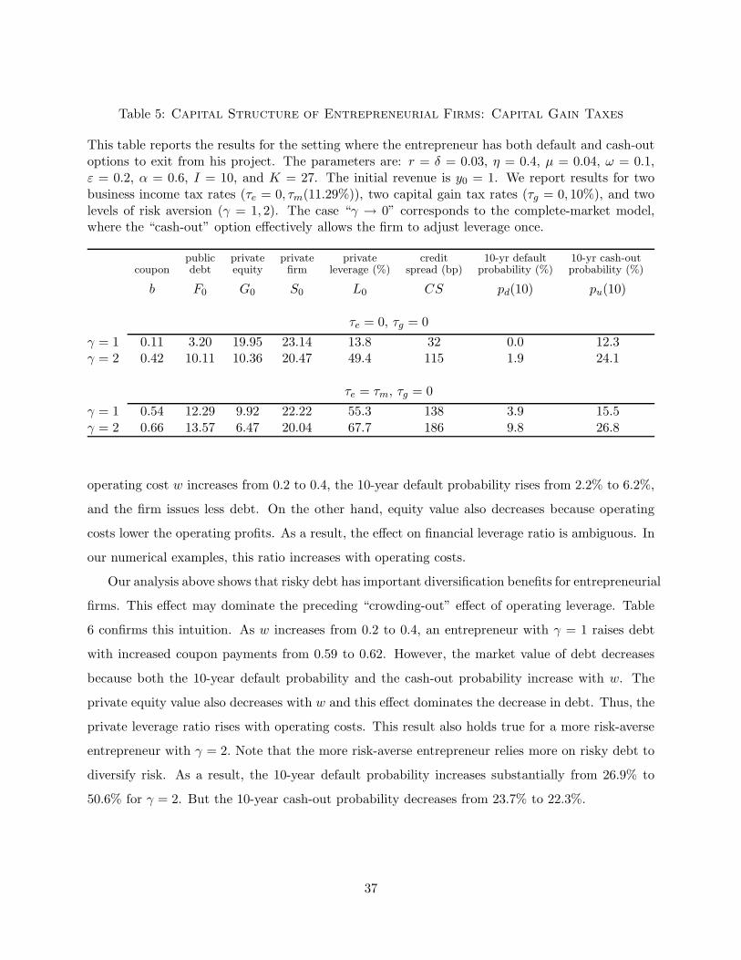
Table 5: Capital Structure of Entrepreneurial Firms: Capital Gain Taxes

This table reports the results for the setting where the entrepreneur has both default and cash-outoptions to exit from his project. The parameters are: r = δ = 0.03, η = 0.4, µ = 0.04, ω = 0.1,ε = 0.2, α = 0.6, I = 10, and K = 27. The initial revenue is y0 = 1. We report results for twobusiness income tax rates (τe = 0, τm(11.29%)), two capital gain tax rates (τg = 0, 10%), and twolevels of risk aversion (γ = 1, 2). The case “γ → 0” corresponds to the complete-market model,where the “cash-out” option effectively allows the firm to adjust leverage once.

public private private private credit 10-yr default 10-yr cash-outcoupon debt equity firm leverage (%) spread (bp) probability (%) probability (%)

b F0 G0 S0 L0 CS pd(10) pu(10)

τe = 0, τg = 0

γ = 1 0.11 3.20 19.95 23.14 13.8 32 0.0 12.3γ = 2 0.42 10.11 10.36 20.47 49.4 115 1.9 24.1

τe = τm, τg = 0

γ = 1 0.54 12.29 9.92 22.22 55.3 138 3.9 15.5γ = 2 0.66 13.57 6.47 20.04 67.7 186 9.8 26.8

operating cost w increases from 0.2 to 0.4, the 10-year default probability rises from 2.2% to 6.2%,

and the firm issues less debt. On the other hand, equity value also decreases because operating

costs lower the operating profits. As a result, the effect on financial leverage ratio is ambiguous. In

our numerical examples, this ratio increases with operating costs.

Our analysis above shows that risky debt has important diversification benefits for entrepreneurial

firms. This effect may dominate the preceding “crowding-out” effect of operating leverage. Table

6 confirms this intuition. As w increases from 0.2 to 0.4, an entrepreneur with γ = 1 raises debt

with increased coupon payments from 0.59 to 0.62. However, the market value of debt decreases

because both the 10-year default probability and the cash-out probability increase with w. The

private equity value also decreases with w and this effect dominates the decrease in debt. Thus, the

private leverage ratio rises with operating costs. This result also holds true for a more risk-averse

entrepreneur with γ = 2. Note that the more risk-averse entrepreneur relies more on risky debt to

diversify risk. As a result, the 10-year default probability increases substantially from 26.9% to

50.6% for γ = 2. But the 10-year cash-out probability decreases from 23.7% to 22.3%.

37

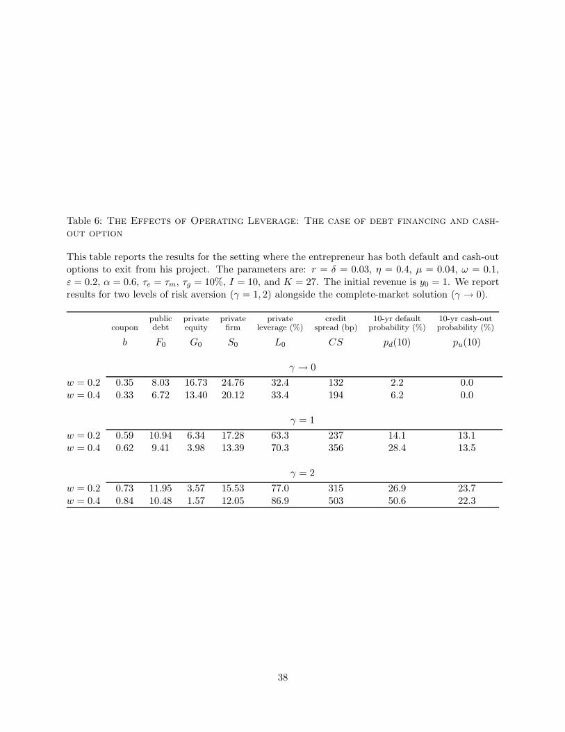
Table 6: The Effects of Operating Leverage: The case of debt financing and cash-out option

This table reports the results for the setting where the entrepreneur has both default and cash-outoptions to exit from his project. The parameters are: r = δ = 0.03, η = 0.4, µ = 0.04, ω = 0.1,ε = 0.2, α = 0.6, τe = τm, τg = 10%, I = 10, and K = 27. The initial revenue is y0 = 1. We reportresults for two levels of risk aversion (γ = 1, 2) alongside the complete-market solution (γ → 0).

public private private private credit 10-yr default 10-yr cash-outcoupon debt equity firm leverage (%) spread (bp) probability (%) probability (%)

b F0 G0 S0 L0 CS pd(10) pu(10)

γ → 0

w = 0.2 0.35 8.03 16.73 24.76 32.4 132 2.2 0.0w = 0.4 0.33 6.72 13.40 20.12 33.4 194 6.2 0.0

γ = 1

w = 0.2 0.59 10.94 6.34 17.28 63.3 237 14.1 13.1w = 0.4 0.62 9.41 3.98 13.39 70.3 356 28.4 13.5

γ = 2

w = 0.2 0.73 11.95 3.57 15.53 77.0 315 26.9 23.7w = 0.4 0.84 10.48 1.57 12.05 86.9 503 50.6 22.3

38

References

Abel, A. B., and J. C. Eberly, 1994, “A unified model of investment under uncertainty,” American

Economic Review, 84, 1369–1384.

Andrade, G., and S. N. Kaplan, 1998, “How Costly is Financial (Not Economic) Distress? Evidence

from Highly Leveraged Transactions That Became Distressed,” Journal of Finance, 53, 1443–

1493.

Attanasio, O. P., 1999, “Consumption,” In: Taylor, J.B., Woodford, M. (Eds.), Handbook of

Macroeconomics, vol. 1B. North-Holland, Amsterdam.

Berger, A. N., and G. F. Udell, 1998, “The economics of small business finance: The roles of

private equity and debt markets in the financial growth cycle,” Journal of Banking & Finance,

22, 613–673.

Berle, A. A., and G. C. Means, 1932, The Modern Corporation and Private Property, Harcourt,

Brace & World, New York.

Bhamra, H. S., L.-A. Kuehn, and I. A. Strebulaev, 2008, “The Levered Equity Risk Premium and

Credit Spreads: A Unified Framework,” Working paper.

Bitler, M. P., T. J. Moskowitz, and A. Vissing-Jrgensen, 2005, “Testing Agency Theory with

Entrepreneur Effort and Wealth,” Journal of Finance, 60, 539–576.

Black, F., and J. Cox, 1976, “Valuing Corporate Securities: Some Effects of Bond Indenture Pro-

visions,” Journal of Finance, 31, 351–367.

Black, F., and M. Scholes, 1973, “The Pricing of Options and Corporate Liabilities,” Journal of

Political Economy, 81, 637–659.

Brav, O., 2009, “Access to Capital, Capital Structure, and the Funding of the Firm,” Journal of

Finance, 64, 263–308.

Brennan, M., and E. S. Schwartz, 1985, “Evaluating natural resource investments,” Journal of

Business, 58, 135–157.

Caballero, R. J., 1991, “Earnings uncertainty and aggregate wealth accumulation,” American Eco-

nomic Review, 81, 859–871.

39

Carpenter, J. N., R. Stanton, and N. Wallace, 2008, “Optimal Exercise of Executive Stock Options

and Implications for Firm Cost,” Working paper.

Chen, H., 2008, “Macroeconomic Conditions and the Puzzles of Credit Spreads and Capital Struc-

ture,” Working Paper.

Cole, R. A., and J. D. Wolken, 1996, “Bank and Nonbank Competition for Small Business Credit:

Evidence from the 1987 and 1993 National Surveys of Small Business Finances,” Federal Reserve

Bulletin, pp. 983–995.

Cox, J. C., and C. Huang, 1989, “Optimum Consumption and Portfolio Policies When Asset Prices

Follow a Diffusion Process,” Journal of Economic Theory, 49, 33–83.

De Nardi, M., P. Doctor, and S. D. Krane, 2007, “Evidence on entrepreneurs in the United States:

data from the 19892004 survey of consumer finances,” Economic Perspectives, pp. 18–36.

Deaton, A., 1992, Understanding Consumption, Oxford University Press, Oxford.

DeMarzo, P. M., and B. Urosevic, 2006, “Ownership Dynamics and Asset Pricing with a Large

Shareholder,” Journal of Political Economy, 114, 774–815.

Dixit, A. K., and R. S. Pindyck, 1994, Investment Under Uncertainty, Princeton University Press,

Princeton, N.J.

Duffie, D., 2001, Dynamic Asset Pricing Theory, Princeton University Press, Princeton, 3rd edn.

Duffie, D., and D. Lando, 2001, “Term Structures of Credit Spreads with Incomplete Accounting

Information,” Econometrica, 69, 633–664.

Dumas, B., 1991, “Super contact and related optimality conditions,” Journal of Economic Dynam-

ics and Control, 4, 675–685.

Fischer, E. O., R. Heinkel, and J. Zechner, 1989, “Dynamic Capital Structure Choice: Theory and

Tests,” Journal of Finance, 44, 19–40.

Gentry, W. M., and R. G. Hubbard, 2004, “Entrepreneurship and Household Saving,” Advances in

Economic Analysis & Policy, 4, 1053–1053.

40

Goldstein, R., N. Ju, and H. Leland, 2001, “An EBIT-Based Model of Dynamic Capital Structure,”

Journal of Business, 74, 483–512.

Graham, J. R., and C. Harvey, 2001, “The Theory and Practice of Corporate Finance: Evidence

from the Field,” Journal of Financial Economics, 60, 187–243.

Hackbarth, D., C. A. Hennessy, and H. E. Leland, 2007, “Can the Trade-off Theory Explain Debt

Structure?,” Review of Financial Studies, 20, 1389–1428.

Hackbarth, D., J. Miao, and E. Morellec, 2006, “Capital Structure, Credit Risk, and Macroeconomic

Conditions,” Journal of Financial Economics, 82, 519–550.

Hall, R. E., 1978, “Stochastic Implications of the Life Cycle-Permanent Income Hypothesis: Theory

and Evidence,” Journal of Political Economy, 86, 971–987.

Hall, R. E., and S. E. Woodward, 2008, “The Burden of the Nondiversifiable Risk of Entrepreneur-

ship,” Working Paper, Stanford University.

Heaton, J. C., and D. J. Lucas, 2004, “Capital Structure, Hurdle Rates, and Portfolio Choice

Interactions in an Entrepreneurial Firm,” Working Paper, Northwestern University.

Jensen, M. C., and W. H. Meckling, 1976, “Theory of the Firm: Managerial Behavior, Agency

Costs and Ownership Structure,” Journal of Financial Economics, 3, 305–360.

Kimball, M., and N. Mankiw, 1989, “Precautionary saving and the timing of taxes,” Journal of

Political Economy, 97, 863–879.

Kimball, M. S., 1990, “Precautionary Saving in the Small and in the Large,” Econometrica, 58,

53–73.

Krylov, N., 1980, Controlled Diffusion Processes, Springer, Berlin.

Leland, H., 1994, “Corporate Debt Value, bond covenants, and Optimal Capital Structure,” Journal

of Finance, 49, 1213–1252.

Leland, H. E., 1968, “Saving and uncertainty: the precautionary demand for savings,” Quarterly

Journal of Economics, 82, 465–473.

41

Leland, H. E., and D. H. Pyle, 1977, “Informational Asymmetrics, Financial Structure, and Finan-

cial Intermediation,” Journal of Finance, 32, 371–387.

McDonald, R., and D. Siegel, 1986, “The value of waiting to invest,” Quarterly Journal of Eco-

nomics, 101, 707–728.

Merton, R. C., 1971, “Optimum Consumption and Portfolio Rules in a Continuous-Time Model,”

Journal of Economic Theory, 3, 373–413.

Merton, R. C., 1973a, “An Intertemporal Capital Asset Pricing Model,” Econometrica, 41, 867–887.

Merton, R. C., 1973b, “Theory of Rational Option Pricing,” Bell Journal of Economics and Man-

agement Science, 4, 141–183.

Miao, J., 2005, “Optimal Capital Structure and Industry Dynamics,” Journal of Finance, 60,

2621–2659.

Miao, J., and N. Wang, 2007, “Investment, Consumption and Hedging under Incomplete Markets,”

Journal of Financial Economics, 86, 608–642.

Miller, M. H., 1977, “Debt and Taxes,” Journal of Finance, 32, 261–275.

Moskowitz, T. J., and A. Vissing-Jorgensen, 2002, “The Returns to Entrepreneurial Investment: A

Private Equity Premium Puzzle?,” American Economic Review, 92, 745–778.

Myers, S. C., and N. S. Majluf, 1984, “Corporate Financing and Investment Decisions when Firms

Have Information That Investors do not Have,” Journal of Financial Economics, 13, 187–221.

Petersen, M. A., and R. G. Rajan, 1994, “The Benefits of Lending Relationships: Evidence from

Small Business Data,” Journal of Finance, 49, 3–37.

Rauh, J. D., 2008, “Risk Shifting versus Risk Management: Investment Policy in Corporate Pension

Plans,” Forthcoming, Review of Financial Studies.

Schumpeter, J., 1934, The Theory of Economic Development: An Inquiry into Profits Capital Credit

Interest and the Business Cycle, Cambridge, MA.

Strebulaev, I. A., 2007, “Do Tests of Capital Structure Theory Mean What They Say?,” Journal

of Finance, 62, 1747–1787.

42

Svensson, L., and I. Werner, 1993, “Nontradeal assets in incomplete markets: pricing and portfolio

choice,” European Economic Review, 37, 1149–1168.

Wang, N., 2006, “Generalizing the Permanent-Income Hypothesis: Revisiting Friedman’s Conjec-

ture on Consumption,” Journal of Monetary Economics, 53, 737–752.

43