1

Paper 2693-2018

Enterprise, Prepare for Analysis! Using SAS® Data Management to Prepare Data for Analysis

Bob Janka, Experis – Business Intelligence and Analytics

ABSTRACT

Data analysis teams often have few resources for many needs. Using SAS® Data Management, we can

integrate enterprise-level data from different sources, cleanse that data, and enrich it for analysis. These

steps reduce the workload for the analysis team, enabling them to focus on the actual analytics. This

paper highlights some uses of enterprise-level tools in SAS® Data Integration Studio and SAS

® Data

Quality in data preparation. Several of the techniques shown are also applicable to users of Base SAS®

(with the SAS® macro facility).

INTRODUCTION

Preparing data is an essential step in analytics. While most readers know Base SAS and SAS Macro, few are familiar with the capabilities inherent in the SAS® Data Management offering. On the other hand, many users of SAS® Data Management might not have backgrounds in analytics. This paper helps bridge the two worlds.

This paper starts with a brief overview of the products in the SAS® Data Management offering, then works through examples of a few common tasks in preparing data for analytics and how those work in SAS® Data Integration Studio.

The Data Management offering provides many capabilites. Full coverage of these exceeds the scope of this paper. Also, this paper focuses on repeatable analyses and does not cover any ad-hoc analyses.

Many of the examples are adapted from concepts discussed in the book, _Data Preparation for Analytics Using SAS®_ , authored by Gerhard Svolba, PhD. 2006. Although the example data and jobs are relatively small, the concepts do scale well to much larger volumes in Data Integration Studio. Each topic includes SAS code to create the input datasets. The author assumes that the reader knows or can learn how to create libnames and register tables in Data Integration Studio.

WHAT IS ENTERPRISE DATA MANAGEMENT?

The primary distinction of Enterprise Data Management is the use of one or more servers to periodically process data on large volumes, typically over a million records per time interval. Most organizations that use Enterprise Data Management have data warehouses that contain multiple datamarts. Examples of these are larger businesses, especially those that generate and store data for many thousands of transactions on a weekly, daily, or even hourly basis. Financial institutions, government entities, large retail companies, and many others all have these data volumes.

SAS® DATA MANAGEMENT

SAS® Data Management comprises 2 major tools to help organizations meet their Enterprise Data Management needs: SAS® Data Integration Studio and SAS® Data Management Studio. The first supports development of jobs to Extract, Transform, and Load (ETL) while the second supports development of jobs to manage data quality.

SAS® DATA INTEGRATION STUDIO

2

Data Integration Studio uses a visual flow, i.e. a graphical user interface (GUI) to build up the steps in each job. It has a wide variety of node types as shown in Table 1.

Access Analysis Archived

Change Data Capture Control Data

Data Quality Hadoop High-Performance Analytics

Output Publish SPD Server Dynamic Cluster

SQL

Table 1. Data Integration Studio node groups

Many of the examples in this paper have a source data node, a transformation node, and a target data node. The examples highlight specific changes to the properties of the transformation node. The displays show three terms: columns, rows, and tables, which most SAS programmers will recognize as variables, observations, and datasets respectively.

Data Integration Studio jobs create SAS code to execute the specified steps. These utilize Base SAS, SAS Macro, and any other SAS Foundation products included with the site license and installed.

This paper refers to two key macro variables, which Data Integration Studio automatically sets in each node: &_INPUT. and &_OUTPUT. In a couple of the examples, the code needs to specify the input and output data sets. By using these variables, user written code can let the node connections specify the actual LIBREF.DATASET values.

SAS® DATA MANAGEMENT STUDIO

Data Management Studio (formerly known as DataFlux Data Management Studio) also uses a visual flow, i.e. a graphical user interface (GUI) to build up the steps in Data Quality jobs. Data Management Studio jobs use a different language, i.e. the Expression Evaluation Language (EEL), instead of SAS. This also means that nodes process data one record at a time.

Data Management Studio covers several areas as described in Table 2. Further details about SAS® Data Management Studio appear in other papers.

Area Example Capabilities

Identification Analysis Determined semantic type of source data values (e.g. name, address, phone)

Locale Guessing Determine locale of source data such as phone number prefixes (e.g., +1 English in US or Can, +49 German in Germany, etc.)

Standardization Adjust input data to standard case, spellings, and/or abbreviations

Parsing Split text strings into constituent parts (e.g., address number,street,city,etc.)

Verification Compare data to external sources, such as the US Post Office address database

Enrichment Add extra information to records via lookup tables and/or joins

Matching Determine likely matches using “fuzzy logic”

Table 2. Data Management Studio areas

DATA PREPARATION FOR ANALYTICS

Analytics require good data preparation. A key assumption in this paper is that there are too few data scientists to handle all of the analysis, much less all of the work involved in analytics. A commonly mentioned statistic is that data scientists spend 80% of their time preparing the data and only about 20% of their time in the actual analyses. This is where other staff, such as data engineers, can help by using their skills in data management to collect and prepare the data into a format that enables analytics.

3

Repeatable analyses as covered in this paper can span a variety of techniques: linear regressions for numerical results, logistic regressions for yes/no analyses, time series, data mining, and many others. It is important for the data engineers to discuss the general techniques with their data scientists in order to better prepare the data for analyses.

For each of five common techniques, this paper briefly introduces the technique, then describes how to implement that technique using Data Integration Studio. These techniques include the following:

Replacing missing data – using the Standardize transformation

Binning or grouping data – using the Rank transformation

Aggregating data – using the Summary Statistics transformation

Deriving data – using the SQL Create Table transformation

Detecting missing data - using the User Written Code transformation

REPLACING MISSING DATA

Missing data can cause many analyses to fail or yield misleading results. A common technique is to replace any missing values with either a constant value, such as 0 or 1, or some computed value, such as the mean or median of the non-missing values. The mean is often used when assuming that the inherent distribution in the source data approximates the normal distribution.

In Data Integration Studio, you use the Standardize transformation. The example job is shown in Display 1.

Display 1. Job to replace missing data using the Standardize transformation.

The data used in this example comes from a small dataset created by this code segment:

data test;

input age @@;

cards; /* aka datalines */

12 60 . 24 . 50 48 34 .

;

run;

For this example, you specify the 1 variable, age, which you want to standardize in the VAR statement. You can see this in Display 2.

4

Display 2. Assign Columns page of Options tab in Standardize transformation.

Using the defaults, the Standardize transformation replaces any missing values in this variable with the mean of the other instances of this variable which have non-missing data. This transformation actually uses an internal SAS macro to run PROC STANDARD. The macro is too large to show in its entirety. See the actual code generated by Data Integration Studio via the macro in Output 1.

915 %Standard;

MPRINT(STANDARD): ODS listing;

MPRINT(STANDARD): options mprint;

MPRINT(STANDARD): proc standard data = DPFA.TEST () out =

DPFA.TEST__STANDARDIZE () replace ;

MPRINT(STANDARD): var AGE;

MPRINT(STANDARD): run;

NOTE: The data set DPFA.TEST__STANDARDIZE has 9 observations and 1

variables.

NOTE: PROCEDURE STANDARD used (Total process time):

real time 0.01 seconds

cpu time 0.00 seconds

916

Output 1. Generated code from SAS log in Standardize transformation

The generated code for PROC STANDARD specifies the default action of “replace”, which tells the PROC to replace missing values with the mean. In this case, PROC STANDARD computes a mean of 38. You can see the results in Output 2, where the previously missing values, which are highlighted, are replaced by the mean.

5

Output 2. View of data results from Standardize transformation.

BINNING OR GROUPING DATA

Another common technique requires binning or grouping data. Some statistical analyses may perform better with only a few categories in lieu of a large number. Binning helps us by grouping the numerical data into a small set of bins.

Data Integration Studio provides the Rank transformation to populate these bins. This transformation generates code using the RANK Procedure. The example takes a table of dates and values, then assigns each observation to one of ten groups. In effect, the code specifies how many groups and PROC RANK figures out the appropriate break values for each group. See the job diagram in Display 3 for details.

Display 3. Job diagram for Binning Data using Rank transformation.

The data for this job is copied from SASHELP as shown here:

data DPFA.air;

set SASHELP.air; /* installed with SAS/ETS */

run;

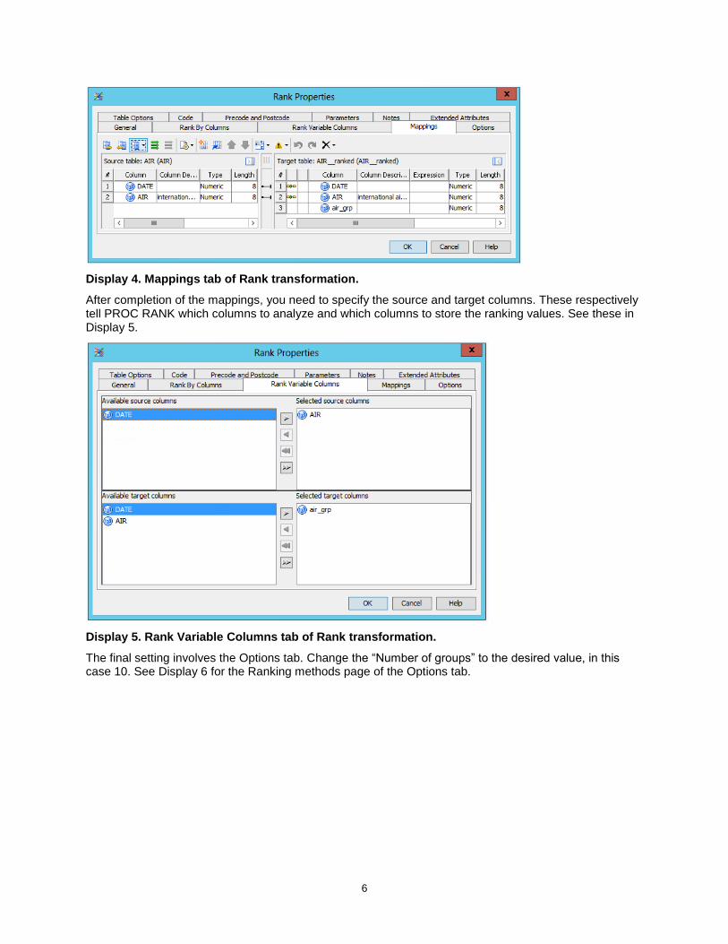
A key feature of this example is the addition of a new column, air_grp, to the target table in the Mappings tab, as shown in Display 4. First, map the two columns in the source table to corresponding columns in the target table. Then, add a new column, air_grp, to the target table which will receive the ranking value. Next, set the type to Numeric with a length of 8.

6

Display 4. Mappings tab of Rank transformation.

After completion of the mappings, you need to specify the source and target columns. These respectively tell PROC RANK which columns to analyze and which columns to store the ranking values. See these in Display 5.

Display 5. Rank Variable Columns tab of Rank transformation.

The final setting involves the Options tab. Change the “Number of groups” to the desired value, in this case 10. See Display 6 for the Ranking methods page of the Options tab.

7

Display 6. Ranking methods page of Options tab in Rank transformation

Finally, look at the generated code below. Note that the Rank transformation first runs PROC DATASETS to delete any previous copies of the target dataset. This clears the way for PROC RANK to produce its output and also helps rebuild the dataset in case you modified the mappings to specify any additional columns.

In the code tab, you would find the following generated code:

proc datasets lib = DPFA nolist nowarn memtype = (data view);

delete AIR__ranked;

quit;

proc rank data = DPFA.AIR

out = DPFA.AIR__ranked

Ties=MEAN

Groups=10;

var AIR;

ranks air_grp;

run;

Now look at the results in Output 3. Note that this only shows rows 13-20 of 144. You can see at least three groups (0, 1, or 2) in the ranking value column, air_grp.

Output 3. Partial view of data results from Rank transformation.

AGGREGATING DATA

The next technique, aggregating data, is very common. Sometimes, there are too many rows or observations in the source data for practical analysis. In other cases, a model may better fit the data if run at a higher level of aggregation than the source data.

Data Integration Studio provides the Summary Statistics transformation which uses the MEANS (or SUMMARY) Procedure in its code generation. This example generates six descriptive statistics for one analysis variable and groups those using a class variable. Display 7 shows the job diagram.

8

Display 7. Job diagram of Aggregating data using the Summary Statistics transformation.

The SAS code to create the LONG dataset is a little more involved for this example. First, load 10 rows with 1 id and 6 monthly values, then transpose those rows to 1 id, 1 month, and 1 value. Finally, set formats and names:

data DPFA.wide;

input CustID M1 M2 M3 M4 M5 M6 8.;

Cards;

1 52 54 58 47 38 22

2 22 24 30 28 31 30

3 100 120 110 115 100 95

4 43 43 43 . 42 41

5 20 29 35 39 28 44

6 16 24 18 25 30 24

7 80 70 60 50 60 70

8 90 95 80 100 100 90

9 47 47 47 47 47 47

10 50 52 0 50 0 52

;

run;

proc transpose data = DPFA.wide out = DPFA.long;

by custid;

run;

data DPFA.long;

set DPFA.long;

format month 8.;

rename col1 = usage;

month = compress(_name_,'m');

drop _name_;

run;

As shown previously in the Rank transformation, start with the mapping tab of the Summary Statistics transformation. You map the column containing the class variable, CustID, from the source table to the target table. Do not map any other columns in the source table. Then create new columns in the target table, one for each descriptive statistic you want in the output. Display 8 shows these columns.

9

Display 8. Mappings tab from Summary Statistics transformation.

Next, specify which columns to use for analysis in the VAR statement of PROC MEANS and which columns to use for classification or grouping in the CLASS statement. See Display 9 for these details.

Display 9. Assign Columns page of Options tab in Summary Statistics transformation.

Then, choose the descriptive statistics. You set these on Statistics, Basic page of the Options tab in the Summary Statistics transformation as shown in Display 10.

10

Display 10. Basic Statistics page of Options tab in Summary Statistics transformation.

One last setting involves a flag on the procedue statement. Since this job will run on a regular basis, you don’t need to capture any output generated by PROC MEANS. On Results page of the Options tab, as shown in Display 11, modify “Suppress all displayed output” to the value of NOPRINT.

Display 11. Results page of Options tab in Summary Statistics transformation.

Like the Standardize transformation discussed above, the Summary Statistics transformation uses an internal SAS macro to build the call to PROC MEANS, then executes it. See code for PROC MEANS in Output 4.

608 %MeansTable

MPRINT(MEANSTABLE): ODS listing;

MPRINT(MEANSTABLE): ;

MPRINT(MEANSTABLE): proc means data = DPFA.LONG () NOPRINT fw=12

printidvars nway MEAN SUM N STD MIN MAX ;

MPRINT(MEANSTABLE): ;

11

MPRINT(MEANSTABLE): class CustID ;

MPRINT(MEANSTABLE): ;

MPRINT(MEANSTABLE): ;

MPRINT(MEANSTABLE): output OUT = DPFA.LONG__smry_stats (drop = _type_

_freq_ _way_) MEAN ()= SUM ()= N ()= STD ()= MIN ()= MAX

()= / autoname autolabel ways inherit ;

MPRINT(MEANSTABLE): ;

MPRINT(MEANSTABLE): ;

MPRINT(MEANSTABLE): var Usage ;

MPRINT(MEANSTABLE): ;

MPRINT(MEANSTABLE): run;

NOTE: There were 60 observations read from the data set DPFA.LONG.

NOTE: The data set DPFA.LONG__SMRY_STATS has 10 observations and 7

variables.

NOTE: The PROCEDURE MEANS printed page 1.

NOTE: PROCEDURE MEANS used (Total process time):

real time 0.06 seconds

cpu time 0.04 seconds

609

Output 4. Generated code for PROC MEANS in Summary Statistics transformation.

The results in Output 6 show ten rows for each of the CustID values and the six corresponding statistics. Note that each CustId had about 6 values of Usage in the source data.

Output 5. View of data results from Summary Statistics transformation.

DERIVING DATA

For some analyses, you need to derive new variables to adjust the data. This is especially true if you need to compute the profit for sales data where you have the costs and sales prices for the individual items. A different analysis might require a shift of the data from a logarithm scale to a linear scale, which this example explores.

While there are several ways to do that in Data Integration Studio, this example uses the SQL Create Table transformation which use the SQL Procedure during its code generation. The job diagram is in Display 12.

12

Display 12. Job diagram for Deriving Data using SQL Create Table transformation

Create the source data:

data skewed;

input a @@;

cards;

1 0 -1 20 4 60 8 50 2 4 7 4 2 1

;

run;

First, choose the source table. Since the SQL Create Transformation allows multiple input tables, the Source tab is separate from the Mapping tab. See this in Display 13.

Display 13. Source tab for SQL Create Table transformation.

Second, specify the mappings in the Result tab as shown in Display 14. This is analagous to the Mappings tab in other transformations. A key difference in this example is that you map one source column to the 3 target columns: one copies the data from the original source column and the other two derive new values from the source data. One new value computes the log() of the source data while the other new value computes the fourth-root of the source data. Since the generated code uses PROC SQL, the computed value can use any expression that Base SAS and any other installed SAS products support. When entering the expressions, type the following and Data Integration Studio adjusts it:

Entered Column Expression (adjusted)

Type Length.

log(a+2) log_a log(SKEWED.a+2) Numeric 8.

(a+2)**(0.25) root4_a (SKEWED.a+2)**(0.25) Numeric 8.

The adjusted expressions explictly specify to PROC SQL which input table contains the source data.

Similar expressions can occur in almost any table mapping. Thus, you can add these derivations to other transformations and possibly eliminate a node dedicated to just the derived values.

13

Display 14. Result tab for SQL Create Table transformation.

Now, review the generated code, which has the 2 expressions highlighted in bold:

proc datasets lib = DPFA nolist nowarn memtype = (data view);

delete SKEWED__log_root__sql;

quit;

proc sql

;

create table DPFA.SKEWED__log_root__sql as

select

SKEWED.a length = 8,

log(SKEWED.a+2) as log_a length = 8,

(SKEWED.a+2)**(0.25) as root4_a length = 8

from

DPFA.SKEWED as SKEWED

;

quit;

Finally, review the data results in Output 6.

Output 6. View of data results from SQL Create Table transformation.

DETECTING MISSING DATA

14

Conceptually, this technique should occur earlier in the data preparation process, before the first technique of Replacing Missing Data. Since it uses an advanced feature of Data Integration Studio, the User Written Code transformation, we discuss it now.

This example invokes a macro that, for each specified variable, counts the number of missing values and sets a flag if the percentage exceeds a specified threshold. The job diagram in Display 15 shows 1 source table and 2 transformations and no target tables. This is because each transformation generates output instead of creating or updating tables.

As shown in the job diagram, Data Integration Studio allows you to connect 1 source table to several transformations. This lets you manage the table metadata once instead of several different places.

Display 15. Job Diagram for Detecting Missing Data using User Written Code transformation.

Copy the data for this job from SASHELP as shown here:

data DPFA.demographics;

set SASHELP.demographics; /* installed with SAS/GRAPH */

run;

This example shows one way to add a SAS Macro to a Data Integration job by including the macro definition just before its invocation. This approach works well for developing and troubleshooting macros.

However, after the developer has completed writing and testing the macro, the organization should add the macro to the SAS macro library for Data Integration and then just invoke the macro as shown further below. Because this example does not generate any target data, there are no changes to the Mappings tab.

Review the user written code here:

/*---- Start of User Written Code ----*/

%MACRO AlertNumericMissing (data=,vars=_NUMERIC_,alert=0.2);

/*

* Macro %AlertNumericMissing() adapted from the book,

* Gerhard Svolba, 2006. _Data Preparation for Analytics Using SAS®_.

* _Cary, NC: SAS Institute, Inc._

*/

PROC MEANS DATA = &data NMISS NOPRINT;

VAR &vars;

OUTPUT OUT = miss_value NMISS=;

RUN;

PROC TRANSPOSE DATA = miss_Value(DROP = _TYPE_)

OUT = miss_value_tp;

RUN;

DATA miss_value_tp;

15

SET miss_value_tp;

FORMAT Proportion_Missing 8.2;

RETAIN N;

IF _N_ = 1 THEN N = COL1;

Proportion_Missing = COL1/N;

Alert = (Proportion_Missing >= &alert);

RENAME _name_ = Variable

Col1 = NumberMissing;

IF _name_ = '_FREQ_' THEN DELETE;

RUN;

TITLE Alertlist for Numeric Missing Values;

TITLE2 Data = &data -- Alertlimit >= &alert;

PROC PRINT DATA = miss_value_tp (drop=_label_); /* SGF18: less output */

RUN;

TITLE;TITLE2;

%MEND;

%AlertNumericMissing( data = &_input., alert=0.5 );

/*---- End of User Written Code ----*/

Display 16 shows the tail portion of this code in the Code tab, which is the only properties tab you need to change for this job.

Display 16. Macro definition end and invocation in Code tab of User Written Code transformation.

After running this job interactively, view the results in Output 7. This shows that there are 197 rows and that two columns have percentage missing >= 0.5: PopPovertypct and PopPovertyYear.

16

Output 7. Output tab after running User Written Code transformation.

CONCLUSION

This paper shows several aspects of SAS Data Integration Studio, such as jobs, transformation nodes, and the many options and settings in those nodes. It also shows five examples of how you can implement common data preparation tasks in SAS Data Integration Studio. These include the following and their key transformations:

replacing missing data : Standardize transformation

binning data : Rank transformation

aggregating data : Summary Statistics transformation

deriving data : SQL Create Table transformation

counting missing values : User Written Code transformation

REFERENCES

Svolba, Gerhard. 2006. Data Preparation for Analysis Using SAS®. Cary, NC: SAS Institute, Inc.

ACKNOWLEDGMENTS

I thank the many people who have helped me during my career, especially two of my current colleagues for their insights and advice:

Chuck Kincaid

Brian Varney

RECOMMENDED READING

Proc SQL: Beyond the Basics Using SAS®

CONTACT INFORMATION

Your comments and questions are valued and encouraged. Contact the author at:

17

Bob Janka, MBA Experis – Business Intelligence and Analytics Bob.Janka@experis.com Bob.Janka@computer.org www.experis.us/analytics www.experis.us/clinical

SAS and all other SAS Institute Inc. product or service names are registered trademarks or trademarks of SAS Institute Inc. in the USA and other countries. ® indicates USA registration.

Other brand and product names are trademarks of their respective companies.