Embed Size (px)
Citation preview

1

ENTANGLEMENT IN THE RELATIVISTIC QUANTUM MECHANICS
A THESIS SUBMITTED TOTHE GRADUATE SCHOOL OF NATURAL AND APPLIED SCIENCES
OFMIDDLE EAST TECHNICAL UNIVERSITY
BY
ENDERALP YAKABOYLU
IN PARTIAL FULFILLMENT OF THE REQUIREMENTSFOR
THE DEGREE OF MASTER OF SCIENCEIN
PHYSICS
JANUARY 2010

Approval of the thesis:
ENTANGLEMENT IN THE RELATIVISTIC QUANTUM MECHANICS
submitted by ENDERALP YAKABOYLU in partial fulfillment of the requirements for thedegree of Master of Science in Physics Department, Middle East Technical University by,
Prof. Dr. Canan OzgenDean, Graduate School of Natural and Applied Sciences
Prof. Dr. Sinan BilikmenHead of Department, Physics
Assoc. Prof. Dr. Yusuf IpekogluSupervisor, Physics Department, METU
Prof. Dr. Namık Kemal PakCo-supervisor, Physics Department, METU
Examining Committee Members:
Prof. Dr. Abdullah VercinPhysics Dept., Ankara University
Assoc. Prof. Dr. Yusuf IpekogluPhysics Dept., METU
Prof. Dr. Namık Kemal PakPhysics Dept., METU
Assoc. Prof. Dr. Sadi TurgutPhysics Dept., METU
Assoc. Prof. Dr. Altug OzpineciPhysics Dept., METU
Date:15 January 2010

I hereby declare that all information in this document has been obtained and presentedin accordance with academic rules and ethical conduct. I also declare that, as requiredby these rules and conduct, I have fully cited and referenced all material and results thatare not original to this work.
Name, Last Name: ENDERALP YAKABOYLU
Signature :
iii
ABSTRACT
ENTANGLEMENT IN THE RELATIVISTIC QUANTUM MECHANICS
Yakaboylu, Enderalp
M.S., Department of Physics
Supervisor : Assoc. Prof. Dr. Yusuf Ipekoglu
Co-Supervisor : Prof. Dr. Namık Kemal Pak
January 2010, 44 pages
In this thesis, entanglement under fully relativistic settings are discussed. The thesis starts
with a brief review of the relativistic quantum mechanics. In order to describe the effects of
Lorentz transformations on the entangled states, quantum mechanics and special relativity are
merged by construction of the unitary irreducible representations of Poincare group on the
infinite dimensional Hilbert space of state vectors. In this framework, the issue of finding
the unitary irreducible representations of Poincare group is reduced to that of the little group.
Wigner rotation for the massive particles plays a crucial role due to its effect on the spin
polarization directions. Furthermore, the physical requirements for constructing the correct
relativistic spin operator is also studied. Then, the entanglement and Bell type inequalities are
reviewed. The special attention has been devoted to two historical papers, by EPR in 1935 and
by J.S. Bell in 1964. The main part of the thesis is based on the Lorentz transformation of the
Bell states and the Bell inequalities on these transformed states. It is shown that entanglement
is a Lorentz invariant quantity. That is, no inertial observer can see the entangled state as
a separable one. However, it was shown that the Bell inequality may be satisfied for the
Wigner angle dependent transformed entangled states. Since the Wigner rotation changes
the spin polarization direction with the increased velocity, initial dichotomous operators can
iv

satisfy the Bell inequality for those states. By choosing the dichotomous operators taking into
consideration the Wigner angle, it is always possible to show that Bell type inequalities can
be violated for the transformed entangled states.
Keywords: entanglement, Lorentz transformation, relativistic spin operator, Wigner rotation
v

OZ
GORELI KUANTUM MEKANIGINDE DOLANIKLIK
Yakaboylu, Enderalp
Yuksek Lisans, Fizik Bolumu
Tez Yoneticisi : Doc. Dr. Yusuf Ipekoglu
Ortak Tez Yoneticisi : Prof. Dr. Namık Kemal Pak
Ocak 2010, 44 sayfa
Bu tezde tamamıyla goreli rejimde dolanıklık problemi uzerinde calısılmıstır. Tez teorik
altyapı icin gereki olan goreli kuantum mekaniginin kısa bir ozeti ile baslamaktadır. Lorentz
donusumlerinin dolanık durumlardaki etkisini tanımlayabilmek icin Poincare grubunun son-
suz boyutlu Hilbert uzayında uniter indirgenemez gosterimlerinin insa edilmesi gerekmekte-
dir. Ozel gorelilik ile kuantum mekanigini birlestiren bu cercevede Poincare grubunun temsil-
lerinin bulunması problemi ”kucuk grup” duzeyine indirgenir. Bu grup kutleli parcacıklarda
Wigner donmesine sebep olur. Bu donme spin polarizasyon yonlerini etkiledigi icin buyuk
bir oneme sahiptir. Daha sonra da, bu tezde goreli spin operatoru icin fiziksel gerekliliklerin
ne oldugu calısılmıstır. Tez dolanıklık ve Bell tipi esitsizlikleri tanımlayarak devam etmek-
tedir. Ilki 1935’te A. Einstein, B. Podolsky ve N. Rosen (EPR) tarafından kaleme alınan ve
digeri 1964’te J.S. Bell tarafından yazılan iki tarihsel makaleye de ozel bir onem verilmistir.
Tezin temel bolumu ise, Bell durumlarının Lorentz donesumlerine ve bu donusen durum-
lar icin Bell esitsizliklerine ayrılmıstır. Bu tezde dolanıklıgın Lorentz donusumleri altında
degismedigi gosterilmistir. Yani, hic bir eylemsiz gozlemci bir dolanık durumu ayrılabilir
bir durum olarak goremez. Fakat, donusturulen durumların Bell esitsizligini ihlal etmesi
hem gozlemcinin hızına hem de parcacıkların hızına baglıdır. Wigner donmesi artan hızla
vi

beraber spin polarizasyonunu etkiledigi icin, baslangıctaki Bell operatorleri Wigner acısına
baglı dolanık durumlar icin Bell esitsizligini saglayabilirler. Wigner acısı dikkate alınarak
secilen Bell operatorleri ile, donusturulen durumlar icin Bell tipi esitsizliklerin her zaman
ihlal edilebilecegi gosterilmistir.
Anahtar Kelimeler: dolanıklık, Lorentz donusumleri, goreli spin operatoru, Wigner donmesi
vii

To my family and Ozge
viii

ACKNOWLEDGMENTS
I am thankful to my supervisor Assoc. Prof. Dr. Yusuf Ipekoglu and I would like to express
my deepest gratitude and thanks to co-supervisor Prof. Dr. Namık Kemal Pak for his valuable
ideas, advices and supervision.
I am also grateful to Assoc. Prof. Dr. B. Ozgur Sarıoglu, Assoc. Prof. Dr. Bayram Tekin,
and Assoc. Prof. Dr. Sadi Turgut for their constructive advice, criticism and willing to help
me all the time.
Finally, I would like to show my gratitude to M. Burak Sahinoglu and D. Olgu Devecioglu
for their supports, and I wish to express my warmest thanks to M. Fazıl Celik and A. Aytac
Emecen for their valuable discussion on the physics and philosophy.
ix

TABLE OF CONTENTS
ABSTRACT . . . . . . . . . . . . . . . . . . . . . . . . . . . . . . . . . . . . . . . . iv
OZ . . . . . . . . . . . . . . . . . . . . . . . . . . . . . . . . . . . . . . . . . . . . . vi
ACKNOWLEDGMENTS . . . . . . . . . . . . . . . . . . . . . . . . . . . . . . . . . ix
TABLE OF CONTENTS . . . . . . . . . . . . . . . . . . . . . . . . . . . . . . . . . x
LIST OF TABLES . . . . . . . . . . . . . . . . . . . . . . . . . . . . . . . . . . . . xii
LIST OF FIGURES . . . . . . . . . . . . . . . . . . . . . . . . . . . . . . . . . . . . xiii
CHAPTERS
1 INTRODUCTION . . . . . . . . . . . . . . . . . . . . . . . . . . . . . . . 1
2 RELATIVISTIC QUANTUM MECHANICS . . . . . . . . . . . . . . . . . 3
2.1 Quantum Mechanics . . . . . . . . . . . . . . . . . . . . . . . . . . 3
2.2 Poincare Algebra . . . . . . . . . . . . . . . . . . . . . . . . . . . 5
2.2.1 Casimir Operators . . . . . . . . . . . . . . . . . . . . . 8
2.3 Relativistic Spin and Position Operators . . . . . . . . . . . . . . . 9
2.4 Single Particle and Unitary Irreducible Representations of the PoincareGroup . . . . . . . . . . . . . . . . . . . . . . . . . . . . . . . . . 11
2.4.1 Single Particle . . . . . . . . . . . . . . . . . . . . . . . . 11
2.4.2 Unitary Irreducible Representations of the Poincare Group 12
2.4.3 Massive and Massless Particles . . . . . . . . . . . . . . . 15
2.4.4 Multi-particle Transformation Rule . . . . . . . . . . . . 16
2.4.5 Wigner Rotation . . . . . . . . . . . . . . . . . . . . . . 17
2.4.6 Lorentz Transformation of a Single Particle . . . . . . . . 18
3 ENTANGLEMENT . . . . . . . . . . . . . . . . . . . . . . . . . . . . . . . 21
3.1 Can Quantum Mechanical Description of Physical Reality Be Con-sidered Complete? . . . . . . . . . . . . . . . . . . . . . . . . . . . 21
3.2 On the Einstein-Poldolsky-Rosen paradox . . . . . . . . . . . . . . 23
x
3.3 Definition of Entanglement . . . . . . . . . . . . . . . . . . . . . . 27
3.3.1 Bipartite Entanglement . . . . . . . . . . . . . . . . . . . 27
3.3.2 von Neumann Entropy . . . . . . . . . . . . . . . . . . . 29
3.3.3 Bell States . . . . . . . . . . . . . . . . . . . . . . . . . . 29
3.4 CHSH Inequality . . . . . . . . . . . . . . . . . . . . . . . . . . . 30
4 LORENTZ TRANSFORMATION OF ENTANGLED STATES AND BELLINEQUALITY . . . . . . . . . . . . . . . . . . . . . . . . . . . . . . . . . 32
4.1 Transformation of Entangled States . . . . . . . . . . . . . . . . . . 32
4.2 Schmidt Decomposition and Its Covariance . . . . . . . . . . . . . . 35
4.3 Correlation Function and Bell Inequality . . . . . . . . . . . . . . . 38
5 CONCLUSION . . . . . . . . . . . . . . . . . . . . . . . . . . . . . . . . . 42
REFERENCES . . . . . . . . . . . . . . . . . . . . . . . . . . . . . . . . . . . . . . 44
xi

LIST OF TABLES
TABLES
Table 2.1 Various classes of four momentum and the corresponding little groups. . . . 16
xii

LIST OF FIGURES
FIGURES
Figure 2.1 Lab frame S , and the boosted frame S ′ . . . . . . . . . . . . . . . . . . . 18
Figure 3.1 Single particle configuration . . . . . . . . . . . . . . . . . . . . . . . . . 24
Figure 3.2 Singlet state configuration [12] . . . . . . . . . . . . . . . . . . . . . . . 25
Figure 3.3 Angles that violates the Bell inequality . . . . . . . . . . . . . . . . . . . 26
Figure 4.1 Zero momentum and boosted frame. . . . . . . . . . . . . . . . . . . . . . 33
Figure 4.2 CHSH values versus velocity of the particles and the boosted frame, β and
β′, respectively. . . . . . . . . . . . . . . . . . . . . . . . . . . . . . . . . . . . 39
xiii
CHAPTER 1
INTRODUCTION
Entanglement is one of the most amazing phenomena of the quantum mechanics. It is proba-
bly the most studied topic recently due to the fact that it is somehow related to a wide range of
research areas from quantum information processing to thermodynamics of the black holes.
It were Einstein, Podolsky and Rosen (EPR) and Schrodinger who first recognized a ”spooky”
feature of quantum mechanics [1], [2]. This feature implies the existence of global states
of composite systems which cannot be written as a product of the states of the individual
subsystems [3]. This feature shows that quantum mechanics has a non local character. In this
respect, this property seems to contradict to postulates of the special relativity.
The main aim of EPR was actually to discuss the ”completeness” of the quantum mechanics.
The underlying assumption of the paper was the locality condition; with this assumption the
quantum mechanics seemed to be an incomplete theory. However, J. S. Bell showed that this
non local property lies at the heart of the quantum mechanics [4].
Due to the contradiction one faces with the postulates of the special relativity in discussing
the issue of locality, to settle those issues one needs to address the same problem in different
inertial frames which move with relativistic speeds. The first article that discusses the entan-
glement in different inertial frames was that of P. M. Alsing and G. J. Milburn [5]. After this
paper, there were numerous studies discussing the Lorentz covariance of the entanglement
and Bell type inequalities.
In this thesis, we study the properties of entangled states and Bell inequalities under Lorentz
transformations. For this purpose we first introduced the theoretical background for the rela-
tivistic quantum mechanics. This part briefly summarizes the quantum mechanics and mainly
1

concentrates on the Poincare group and its unitary irreducible representations. Constructing
the representation of the Poincare group in the Hilbert space of the single particle states re-
duces to that of the little group. It is shown that Wigner rotation play crucial role for the
entangled states. Moreover in this part, we have discussed the physical requirements of the
spin operator in detail due to the fact that there are some ambiguities on what the correct
relativistic spin operator is. Then, in the third chapter, we have devoted a special attention on
the two historical papers [1] and [4] for defining the entanglement, and then we have given
a more formal definitions of entanglement and written the Bell type inequalities in a more
elegant way. The next chapter forms the main part of the thesis in which we have investigated
the Lorentz transformation of entangled states and discussed the CHS H inequality for the
transformed states. Finally, the last chapter is devoted to the summary of the conclusions.
2

CHAPTER 2
RELATIVISTIC QUANTUM MECHANICS
Any physical theory which claims to describe the nature fully at all scales and speeds must
obey the rules of both quantum mechanics and the special theory of relativity. This fundamen-
tal unification can be attained via fields or point particles. Although the main stream starts
from the field concept, both ways end up with probably the most ”beautiful” theory of the
physics, that is the quantum field theory. Due to the our specific problem, we have preferred
the second way by following the Weinberg’s well known book [6]. Therefore, we have to start
with quantum mechanics and Poincare algebra which includes all the aspects of the special
relativity.
2.1 Quantum Mechanics
Quantum mechanics can be briefly summarized as follows in the generalized version of Dirac.
1 Physical states are represented by rays in a kind of complex vector space, called Hilbert
space such that if |α〉 and |β〉 are state vectors, then so is a|α〉+b|β〉 for arbitrary complex
numbers a and b. If we define |φ〉 =∑
n an|αn〉 and |ψ〉 =∑
n bn|βn〉, then one can
introduce the inner product complex number in this space such that
〈φ|ψ〉 = 〈ψ|φ〉∗
〈φ|ψ〉 =∑n,m
a∗nbm〈αn|βm〉 (2.1)
〈φ|φ〉 ≥ 0 and vanishes if and only if |φ〉 = 0.
A ray is a set of normalized vectors 〈ψ|ψ〉 = 1 with |ψ〉 and |ψ′〉 belonging to the same
ray if |ψ′〉 = ζ |ψ〉, where ζ is an arbitrary complex number with |ζ | = 1. As a result, |ψ〉
3

and |ψ′〉 represent same physical state.
2 Observables are represented by Hermitian operators which are mappings |ψ〉 → A|ψ〉
of Hilbert space into itself, linear in the sense that
A(a|α〉 + b|β〉
)= aA|α〉 + bA|β〉, (2.2)
and satisfying the reality condition(〈α|
)(A|β〉
)=
(〈α|A†
)(|β〉
). (2.3)
If state vectors |ψ〉 are eigenvectors of an operator A, then state has a definite value for
this observable
A|ψn〉 = an|ψn〉. (2.4)
For the Hermitian operator A, an are real and 〈ψn|ψm〉 = δnm.
3 Measurement are described by a collection of measurement operators {Mm} where m
refers to outcomes measurement that may occur in the experiment and satisfying the
completeness relation such that ∑m
M†mMm = I. (2.5)
Just before the measurement, if the state is |ψ〉, then probability of getting the result m
just after the measurement is
p(m) = 〈ψ|M†mMm|ψ〉∑
m
p(m) = 1 (2.6)
and initial state collapses toMm|ψ〉√
p(m). (2.7)
Special case of the measurements defined here is the projective measurement. Any
observable can be written in spectral decomposition form
A =∑
m
amPm (2.8)
where am are the eigenvalues and Pm = |αm〉〈αm| are corresponding projectors and |αm〉
is the eigenstate of the observable A such that A|αm〉 = am|αm〉.
For the projective measurement, the result of the measurement is one of the eigenvalues
of the observable A with the probability
p(am) = |〈αm|ψ〉|2, (2.9)
and the collapsed state after the measurement is the corresponding eigenvector.
4
4 Total Hilbert space of multi partite system consisting of n subsystems is a tensor product
of the subsystem spaces
H =
n⊗l=1
Hl. (2.10)
In addition to these postulates, it must be defined that if a physical system is represented by
state vector |ψ〉 and |ψ〉′ in different but equivalent frames, then transformation between these
two frames must be performed by either a unitary and linear or anti-unitary and anti-linear
transformations due to the conservation of probability, which is proven by Wigner [7].
|ψ〉′ → |ψ〉 (2.11)
|ψ〉′ = U |ψ〉
2.2 Poincare Algebra
According to Einstein’s principle of relativity if xµ and x′µ are two sets of coordinates in
inertial frames S and S ′, then they are related as x′µ = Λµνxν + aµ. The physical requirement
relating these two sets are the invariance of the infinitesimal intervals:
ηµνdx′µdx′ν = ηµνdxµdxν (2.12)
where η = diagonal(+1,−1,−1,−1). This invariance of the interval imposes the following
constraints on the transformation coordinates
ηµνΛµαΛν
β = ηαβ. (2.13)
This transformation is called Poincare transformation or inhomogeneous Lorentz transforma-
tion. When aµ = 0 then this transformation reduces to homogeneous Lorentz transformation.
It can be easily shown that these transformations form a group, as briefly summarized below:
• Closure:
let x′ = Λ1x + a1 and x′′ = Λ2x′ + a2, then
x′′ = Λ2(Λ1x + a1) + a2
= Λ2Λ1x + Λ2a1 + a2 = Λ3x + a3.
As a result (Λ2, a2)(Λ1, a1) = (Λ2Λ1,Λ2a1 + a2).
5
• Identity:
I = (I, 0)
• Inverse:
(Λ2, a2)(Λ1, a1) = (Λ2Λ1,Λ2a1 + a2) = (I, 0)
⇒ Λ2 = Λ−11 and a2 = −Λ2a1 = −Λ−1
1 a1
As a result inverse of (Λ, a) is (Λ−1,−Λ−1a).
• Associativity:
(Λ2, a2)[(Λ1, a1)(Λ, a)] = [(Λ2, a2)(Λ1, a1)](Λ, a)
Furthermore, this group can be restricted further by the choice of sign of both the determinant
and the ”00” component of the Λ as the follows: take the determinant of both sides of (2.13),
and get
(DetΛ)2 = 1
which leads to DetΛ = 1 or DetΛ = −1. Next, considering the ”00” element of η00 in (2.13),
(Λ00)2 − (Λ0
i)2 = 1
which means that (Λ00)2 ≥ 1. The possible solutions are (Λ0
0) ≥ 1 or (Λ00) ≤ −1.
The Lorentz group that satisfies the DetΛ = 1 and (Λ00) ≥ 1 is called proper orthochronous
Lorentz group and any Lorentz transformation that can be obtained from identity must belong
to this group. Thus the study of the entire Lorentz group reduces to the study of its proper
orthochronous subgroup. Hereafter, we will deal only with inhomogeneous or homogenous
proper orthochronous Lorentz group.
The infinitesimal transformation for the inhomogeneous Lorentz group now can be written as
Λµν = δµν + ωµν, aµ = εµ
Then, one get from (2.13)
ηνµ = ηµν + ωµν + ωνµ + O(ω2)
which implies that ωµν = −ωνµ; note that ωµν = ηµρωρν.
6
This transformation can be represented by U(Λ, a)
U(Λ, a)xµU−1(Λ, a) = Λµνxν + aµ.
For an infinitesimal transformation U(Λ, a) can be parameterized as
U(1 + ω, ε) = 1 +i2ωµνMµν − iεµPµ + · · · (2.14)
Here, Mµν and Pµ are the generators of the homogeneous Lorentz transformations and trans-
lations respectively. Since ωµν is antisymmetric, Mµν can be taken antisymmetric also. One
can easily show that U(Λ, a) also form a group. Then, it follows
U(Λ, a)U(1 + ω, ε)U−1(Λ, a) = U(Λ(1 + ω)Λ−1,Λε − ΛωΛ−1a)
U(Λ, a)(1 +
i2ωµνMµν − iεµPµ
)U−1(Λ, a) = 1 +
i2
(ΛωΛ−1)µνMµν − i(Λε − ΛωΛ−1a)µPµ.
We can now read of the transformation rules of the generators of the Poincare group, from
this equation:
U(Λ, a)MρσU−1(Λ, a) = ΛµρΛν
σ(Mµν − aµPν + aνPµ)
U(Λ, a)PρU−1(Λ, a) = ΛµρPµ. (2.15)
For the infinitesimal transformations as Λµν = δ
µν + ω
µν , and using (2.14) we get
i[Mµν,Mρσ] = ηνρMµσ − ηµρMνσ − ησµMρν + ησνMρµ
i[Pµ,Mρσ] = ηµρPσ − ηµσPρ (2.16)
[Pµ, Pρ] = 0.
This is the Lie algebra of the Poincare group.
Let’s define P0 as Hamiltonian, Pi as three-momentum, Ki = M0i as boost three-vector, and
Ji = εi jkM jk as the total angular momentum three-vector. In terms of these, the Lie algebra
becomes
[Ji, P j] = iεi jkPk,
[Ji, J j] = iεi jkJk,
[Ji,K j] = iεi jkKk,
[Pi, P j] = [Ji, P0] = [Pi, P0] = 0,
[Ki,K j] = −iεi jkJk,
[Ki, P j] = −iδi jP0,
[Ki, P0] = −iPi.
7

As one can see from the commutator of [Ji, J j] = iεi jkJk, transformation generated by Ji forms
also a group which is the three dimensional rotation group, S O(3), and it is the subgroup of
the Poincare group. However the boost generators do not form a group and this is the reason
of the famous Thomas precession.
Poincare group is a connected Lie group, which means that each element of the group is
connected to the identity by a path within the group, but is not compact since the velocity can
not take the c value after boost transformations.
A well known theorem states that any non-compact Lie group has no finite dimensional uni-
tary representation. It has unitary representations in the infinite dimensional space.
As a result representations of the Poincare group on the state vectors in the infinite dimen-
sional Hilbert space is unitary:
|ψ〉′ = U(Λ, a)|ψ〉 (2.17)
and in order U(1 + ω, ε) given in (2.14) to be unitary, all the generators Mµν and Pµ must be
Hermitian.
2.2.1 Casimir Operators
A Casimir operator is an operator which commutes with any element of the corresponding Lie
algebra. Furthermore, if one finds all the independent Casimir operators for an algebra, then
the representation of this algebra in the space of eigenvectors of these Casimir operators will
be irreducible. In other words, classification of the irreducible representations of a Lie group
reduces to finding of a complete set of Casimir operators and calculating the eigenvalues of
these operators.
In [8], it is shown that Poincare group has two independent Casimir operators which are
c1 = P2 = PµPµ, (2.18)
c2 = W2 = WµWµ (2.19)
where Wµ = −12εµνρσMνρPσ is the Pauli-Lubanski Vector.
8
Components of the Pauli-Lubanski vector are
W0 = −12ε0i jkMi jPk
= J · P (2.20)
and
W i = −12εiνρσMνρPσ
= −12εi jk0M jkP0 −
12εiνρ jMνρP j
=12εi jkM jkP0 −
12εi0k jM0kP j −
12εik0 jMk0P j
= JiP0 + εik jM0kP j (2.21)
= JiP0 − εi jkP jKk.
In this thesis we concentrate on the entanglement in the massive particles. For a massive
particle, one can go to the rest frame where Pµ = (m, 0); then, in that frame
W0 = 0 (2.22)
W i = mS i (2.23)
where we defined the spin S i as the value of total angular momentum Ji in the rest frame.
Thus we get,
c1 = P2 = m2 (2.24)
c2 = W2 = −m2S2. (2.25)
From c2 one can obtain two very important results. First, S2 is Lorentz invariant which means
that spin-statistics is frame independent, and second, relativistic spin operator is related to the
Pauli-Lubanski vector.
As a result, for the massive case mass and spin are two fundamental invariants of the Poincare
group that do not change in all equivalent inertial frames.
2.3 Relativistic Spin and Position Operators
Before defining the spin and position operators the physical requirements about these opera-
tors can be given as,
9
1 First of all, the square of the three-spin operator must be Lorentz invariant, i.e, one can
not change the spin-statistics by applying Poincare transformation.
2 Due to the similar structure to the total angular momentum, S must be pseudovector
just like J. In other words S do not change sign under Parity transformation, and should
satisfy the usual commutation, like any three vector
[Ji, S j] = iεi jkS k.
3 Components of spin operator must satisfy the SU(2) algebra, i.e,
[S i, S j] = iεi jkS k
4 Spin can be measured simultaneously with momentum and position operator
[S,P] = [S,Q] = 0
5 Components of position operator must satisfy the canonical commutation relations
[Qi, P j] = iδi j
6 Position operator must be true vector. i.e, it must change sign under parity transforma-
tion and
[Ji,R j] = iεi jkRk.
It was shown in [9] that the spin operator that satisfies all these requirements is
S =Wm−
W0Pm(m + P0)
(2.26)
=P0Jm−
P ×Km−
P(P · J)(P0 + m)m
and the position operator is
Q = −P−10 K −
iP2P2
0
−P ×W
mP0(m + P0)(2.27)
= −12
(P−10 K + KP−1
0 ) −P × S
P0(m + P0)
which is the Newton-Wigner position operator. In reference [9], it is shown that these opera-
tors are unique.
10

2.4 Single Particle and Unitary Irreducible Representations of the Poincare
Group
A state vector of a free particle must transform according to an irreducible unitary represen-
tation of the Poincare group. Then one can determine completely the behavior of the free
particle in the four dimensional Minkowski space-time. In Poincare group, every irreducible
representation corresponds to an elementary particle. As a result particles are classified in
terms of their irreducible representation of Poincare group which may unified with the dis-
crete symmetries such as C,P,T as in the case of the Dirac particle.
2.4.1 Single Particle
In the previous section two Casimir invariants have been defined. Now we can define the
single free massive particle as an eigenstate of the complete set:
m2,S2, S z,P, P0 (2.28)
which is
|m, s, σ,p, p0〉 = |p, σ〉. (2.29)
The eigenvalues of these operator are defined as
m2|p, σ〉 = m2|p, σ〉, (2.30)
S2|p, σ〉 = s(s + 1)|p, σ〉, (2.31)
S z|p, σ〉 = σ|p, σ〉, (2.32)
P|p, σ〉 = p|p, σ〉, (2.33)
P0|p, σ〉 = ωp|p, σ〉 (2.34)
where ωp =√
m2 + p2 and the normalization of the single particle state is set to
〈p′, σ′|p, σ〉 = δσσ′δ(p′ − p). (2.35)
Before proceeding further, we would like to first introduce ladder operators for the spin- 12 for
future use. Since we know the algebra of the spin operators and the eigenstates of S2 and S z,
one can define the ladder operator in the usual manner:
S ± = S x ± iS y (2.36)
11

and
S ±|p, σ〉 =√
s(s + 1) − σ(σ ± 1)|p, σ ± 1〉. (2.37)
As a result one can define eigenstates of the S x and S y as
|p, σx = ±12〉 =
1√
2
(|p,
12〉 ± |p,−
12〉
), (2.38)
|p, σy = ±12〉 =
1√
2
(|p,
12〉 ± i|p,−
12〉
). (2.39)
Since the resolution of identity can be given as,
I =
∫d3p
∑σ
|p, σ〉〈p, σ| (2.40)
then, the spectral decomposition of S i in the basis of S z can be found as
S z =12
∫d3p
(|p,
12〉〈p,
12| − |p,−
12〉〈p,−
12|
), (2.41)
S x =12
∫d3p
(|p,
12〉〈p,−
12| + |p,−
12〉〈p,
12|
), (2.42)
S y =12
∫d3p
(−i|p,
12〉〈p,−
12| + i|p,−
12〉〈p,
12|
). (2.43)
As a result one can conclude that
{S i, S j} =δi j
2(2.44)
and using (2.3), one can obtain also
S iS j =δi j
2+ iεi jkS k. (2.45)
For practical purposes it is better to define the normalized spin operator, S Ni to satisfy
S Ni S N
j = δi j + iεi jkS Nk . (2.46)
2.4.2 Unitary Irreducible Representations of the Poincare Group
Let x′µ = Λµνxν+aµ then, in general the transformation is represented by the unitary operator
as
U(Λ, a) = U(I, a)U(Λ, 0)
on the Hilbert space. Under translation U(I, a), the state vector transforms as
U(I, a)|p, σ〉 = e−ipµaµ |p, σ〉. (2.47)
12
The homogeneous Lorentz transformation which is U(Λ, 0) = U(Λ), produces an eigenvector
of the four momentum with eigenvalue Λp as follows,
PµU(Λ)|p, σ〉 = U(Λ) U−1(Λ)PµU(Λ)︸ ︷︷ ︸Λ−1
ρµPρ
|p, σ〉
= Λ−1ρµU(Λ)Pρ|p, σ〉
= Λ−1ρµU(Λ)pρ|p, σ〉
= ΛµρpρU(Λ)|p, σ〉
= (Λp)µU(Λ)|p, σ〉.
This means that U(Λ)|p, σ〉 must be linear combination of |Λp, σ〉 ,i.e,
U(Λ)|p, σ〉 =∑σ′
Cσ′σ(Λ, p)|Λp, σ′〉. (2.48)
Consider pµ = Lµν(p)kν where kν is four momentum of particle in its rest frame and L some
Lorentz transformation connecting this frame an arbitrary one in which the particle is moving
with momentum p. Thus, it will depend on p. Transformation of the state is then,
|p, σ〉 = N(p)U(L(p))|k, σ〉 (2.49)
where N(p) is the normalization factor which must satisfy (2.35). The procedure for defining
N(p) is the following. First, it can be required that
〈k′, σ′|k, σ〉 = δσ′σδ(k′ − k).
Then
〈p′, σ′|p, σ〉 = |N(p)|2δσ′σδ(k′ − k).
It must also satisfy (2.35). Therefore
|N(p)|2δ(k′ − k) = δ(p′ − p)
To be able to find the |N(p)|2, it is necessary to define the relation between δ(k′ − k) and
δ(p′ − p). For this purpose, the Lorentz invariant integral for an arbitrary function f (p) with
the conditions p2 = m2 and p0 > 0 can be defined as∫d4 pδ(p2 − m2)θ(p0) f (p) (2.50)
13
where θ(p0) is the step function. Then, the equation can be simplified as∫d4 pδ(p2 − m2)θ(p0) f (p) =
∫d3pdp0δ(p02
− p2 − m2)θ(p0) f (p0,p)
=
∫d3pdp0 δ(p0 −
√p2 + m2) + δ(p0 +
√p2 + m2)
2√
p2 + m2θ(p0) f (p0,p)
=12
∫d3p
f (√
p2 + m2,p)√p2 + m2
.
In other words, ∫f (p)
d3p√p2 + m2
(2.51)
is a Lorentz invariant integral. From this result, one can also find the Lorentz invariant delta
function as ∫d3p′ f (p′)δ(p′ − p) =
∫f (p′)
(√p2 + m2δ(p′ − p)
)d3p′√p2 + m2
.
In this equation,√
p2 + m2δ(p′ − p) must be Lorentz invariant. Thus
p0δ(p′ − p) = k0δ(k′ − k) (2.52)
must hold. As a result, we can define
N(p) =
√k0
p0 . (2.53)
Then, (2.54) becomes
|p, σ〉 =
√k0
p0 U(L(p))|k, σ〉. (2.54)
If we apply the Lorentz transformation to the state |p, σ〉 expended in terms of |k, σ〉 as in
(2.54), we get
U(Λ)|p, σ〉 =
√k0
p0 U(Λ)U(L(p))|k, σ〉
=
√k0
p0 U(ΛL(p))|k, σ〉
=
√k0
p0 U(L(Λp))U(L−1(Λp))U(ΛL(p))|k, σ〉
=
√k0
p0 U(L(Λp))U(L−1(Λp)ΛL(p))|k, σ〉.
14

where we have inserted the identity, U(L(Λp))U(L−1(Λp)) = I in the third line. We next
define W = L−1(Λp)ΛL(p). One can obviously see that W does not change k, i.e, Wµνkν = kµ.
This is called the little group [10]. As a result the state transformation under W is
U(W)|k, σ〉 =∑σ′
Dσ′σ(W)|k, σ′〉 (2.55)
where D(W) is the little group representation of U(W) on the state. Using (2.55) in U(Λ)|p, σ〉
we get
U(Λ)|p, σ〉 =
√k0
p0 U(L(Λp))U(W)|k, σ〉
=
√k0
p0
∑σ′
Dσ′σ(W) U(L(Λp))|k, σ′〉︸ ︷︷ ︸|Λp, σ′〉√k0/(Λp)0
=
√(Λp)0
p0
∑σ′
Dσ′σ (W(Λ, p)) |Λp, σ′〉. (2.56)
Thus, to transform the state one should find the little group representations for the Lorentz
group. This means that finding the Cσ′σ is now reduced to finding the Dσ′σ. This method is
called method of induced representations.
2.4.3 Massive and Massless Particles
In this thesis, we are only interested in massive particles. Unitary representation of the Lorentz
group is determined by the little group of the massive particle. Since the W leaves invariant
the kµ, and in the Lorentz group, only three dimensional rotation can leave the kµ invari-
ant. As a result Dσ′σ is the unitary representation of the SO(3); which is exactly the spin-s
representation of the SU(2) and it can defined as:
Dsσ′σ(W) = 〈s, σ′|eiJ·nθW |s, σ〉
Ds=1/2(W) = 1 cosθW
2+ i(σ · n) sin
θW
2(2.57)
where θW is the Wigner angle.
However for the massless case, the group that leaves the kµ invariant is the ISO(2). This is the
group of Euclidean geometry, which includes rotations and translations in two dimensions.
For this case, the little group representation reduces to
Dσ′σ(W) = eiθWσδσ′σ. (2.58)
15

Table 2.1: Various classes of four momentum and the corresponding little groups.
Standard kµ Little Groupa) p2 = m2 > 0, p0 > 0 (m, 0, 0, 0) S O(3)b) p2 = m2 > 0, p0 < 0 (−m, 0, 0, 0) S O(3)c) p2 = 0, p0 > 0 (κ, 0, 0, κ) IS O(2)d) p2 = 0, p0 < 0 (−κ, 0, 0, κ) IS O(2)e) p2 = −κ2 < 0 (0, 0, 0, κ) S O(3)f) pµ = 0 (0, 0, 0, 0) S O(3, 1)
In the table (2.1), only a), c), and f) have physical meanings, and pµ = 0 case describes the
vacuum. Further information about the structure of the Poincare group can be found in [6].
2.4.4 Multi-particle Transformation Rule
First, multi-particle state can be defined as
|p1, σ1; p2, σ2; · · · 〉.
Therefore, one can transform the multi-particle state similar to one-particle state such that
U(Λ)|p1, σ1; p2, σ2; · · · 〉 =
√(Λp1)0(Λp2)0 · · ·
p01 p0
2 · · ·
∑σ′1σ
′2···
Dσ′1σ1 Dσ′2σ2 · · · |Λp1, σ′1; Λp2, σ
′2; · · · 〉
(2.59)
We now define the states with the help of creation operators
|p, σ〉 = a†(p, σ)|0〉 (2.60)
where |0〉 is the Lorentz invariant vacuum state. Then (2.59) can be written in terms of creation
operators as
U(Λ)a†(p1, σ1)a†(p2, σ2) · · · |0〉
=
√(Λp1)0(Λp2)0 · · ·
p01 p0
2 · · ·
∑σ′1σ
′2···
Dσ′1σ1 Dσ′2σ2 · · · a†(Λp1, σ
′1)a†(Λp2, σ
′2) · · · |0〉. (2.61)
Then form (2.61) one gets
U(Λ)a†(p, σ)U−1(Λ) =
√(Λp)0
p0
∑σ′
Dσ′σ (W(Λ, p)) a†(Λp, σ′). (2.62)
For the massive particle it is equivalent to
U(Λ)a†(p, σ)U−1(Λ) =
√(Λp)0
p0
∑σ′
Dsσ′σ (W(Λ, p)) a†(Λp, σ′). (2.63)
16
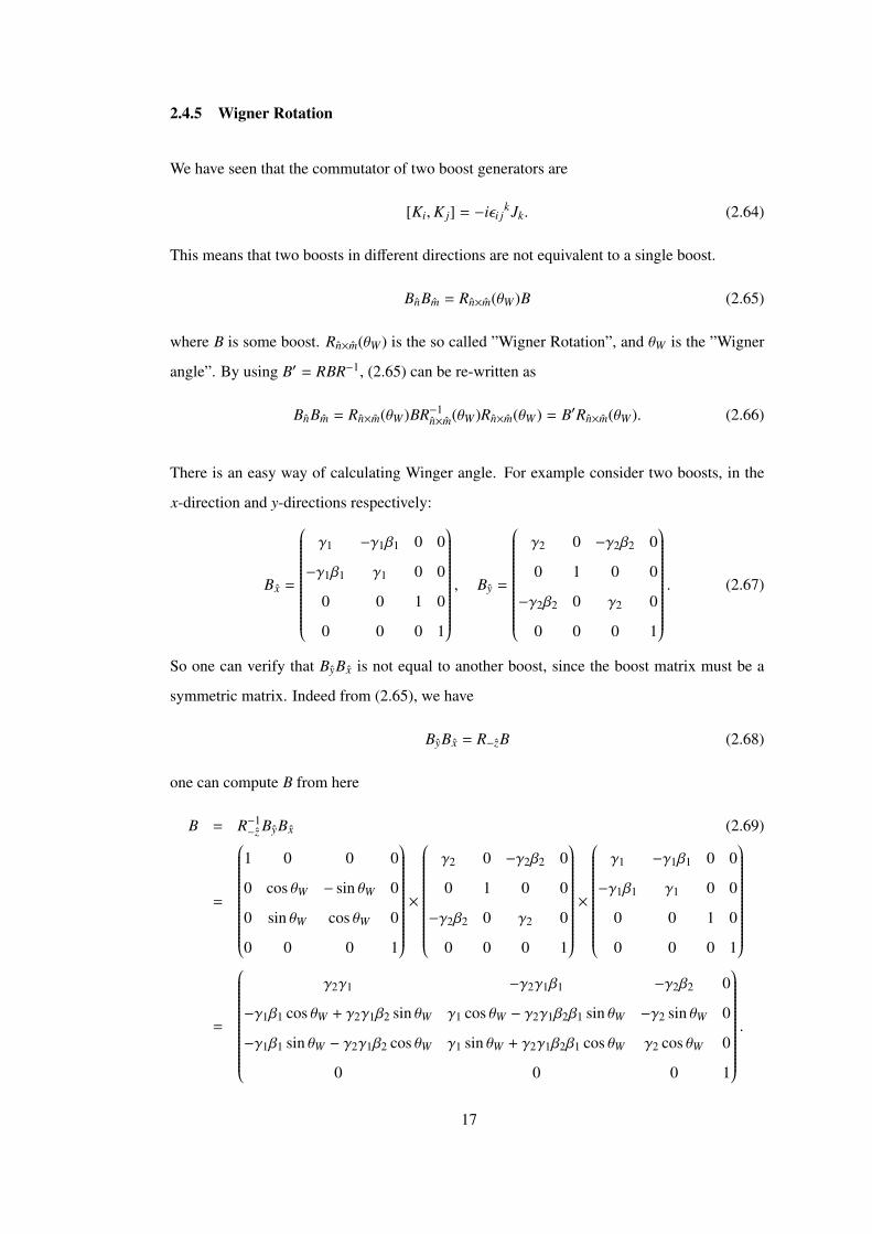
2.4.5 Wigner Rotation
We have seen that the commutator of two boost generators are
[Ki,K j] = −iεi jkJk. (2.64)
This means that two boosts in different directions are not equivalent to a single boost.
BnBm = Rn×m(θW)B (2.65)
where B is some boost. Rn×m(θW) is the so called ”Wigner Rotation”, and θW is the ”Wigner
angle”. By using B′ = RBR−1, (2.65) can be re-written as
BnBm = Rn×m(θW)BR−1n×m(θW)Rn×m(θW) = B′Rn×m(θW). (2.66)
There is an easy way of calculating Winger angle. For example consider two boosts, in the
x-direction and y-directions respectively:
Bx =
γ1 −γ1β1 0 0
−γ1β1 γ1 0 0
0 0 1 0
0 0 0 1
, By =
γ2 0 −γ2β2 0
0 1 0 0
−γ2β2 0 γ2 0
0 0 0 1
. (2.67)
So one can verify that ByBx is not equal to another boost, since the boost matrix must be a
symmetric matrix. Indeed from (2.65), we have
ByBx = R−zB (2.68)
one can compute B from here
B = R−1−z ByBx (2.69)
=
1 0 0 0
0 cos θW − sin θW 0
0 sin θW cos θW 0
0 0 0 1
×
γ2 0 −γ2β2 0
0 1 0 0
−γ2β2 0 γ2 0
0 0 0 1
×
γ1 −γ1β1 0 0
−γ1β1 γ1 0 0
0 0 1 0
0 0 0 1
=
γ2γ1 −γ2γ1β1 −γ2β2 0
−γ1β1 cos θW + γ2γ1β2 sin θW γ1 cos θW − γ2γ1β2β1 sin θW −γ2 sin θW 0
−γ1β1 sin θW − γ2γ1β2 cos θW γ1 sin θW + γ2γ1β2β1 cos θW γ2 cos θW 0
0 0 0 1
.
17

From symmetry properties of the boost matrix, we have−γ2 sin θW = γ1 cos θW−γ2γ1β2β1 sin θW ,
and finally
tan θW =−γ2γ1β2β1
γ2 + γ1(2.70)
is the Wigner angle.
2.4.6 Lorentz Transformation of a Single Particle
We have defined the Wigner rotation as W = L−1(Λp)ΛL(p). Here L(p) is the boost which
transforms the four-momentum kµ to some standard pµ. Since we take the kµ in the particle’s
rest frame, then the components of L(p) are obtained as [6],
Lik(p) = δik + (γ − 1) pi pk (2.71)
Li0(p) = L0
i(p) = pi
√γ2 − 1 (2.72)
L00(p) = γ where pi ≡
pi
|p|, γ =
√p2 + m2/m. (2.73)
To able to determine the Wigner angle, first it is necessary to specify our situation. We have
spin- 12 particle moving in the z-direction relative to the Lab frame, S and there is another
frame, S ′ which is boosted in in the x-direction relative to the S -frame as shown in the figure
(2.1). As a result L(p)z is
Figure 2.1: Lab frame S , and the boosted frame S ′
18

L(p)z =
γ 0 0√γ2 − 1
0 1 0 0
0 0 1 0√γ2 − 1 0 0 γ
(2.74)
where γ is the rapidity and the Λx is
Λx =
coshα sinhα 0 0
sinhα coshα 0 0
0 0 1 0
0 0 0 1
(2.75)
where coshα = γ′ and sinhα = −γ′β′.
Then the Wigner rotation is,
W = L−1(Λp)ΛL(p)
ΛL(p) = L(Λp)W (2.76)
more explicitly
ΛxL(p)z = L(Λp)W−y(θW)
ΛxL(p)zW−1−y (θW) = L(Λp). (2.77)
Then, we get
L(Λp) = ΛxL(p)zW−1−y (θW) = (2.78)
coshα sinhα 0 0
sinhα coshα 0 0
0 0 1 0
0 0 0 1
γ 0 0√γ2 − 1
0 1 0 0
0 0 1 0√γ2 − 1 0 0 γ
1 0 0 0
0 cos θW 0 sin θW
0 0 1 0
0 − sin θW 0 cos θW
=
γ coshα sinhα cos θW +√γ2 − 1 sin θW coshα 0 − sinhα sin θW +
√γ2 − 1 cos θW coshα
γ sinhα√γ2 − 1 sinhα sin θW + cos θW coshα 0 − coshα sin θW +
√γ2 − 1 cos θW sinhα
0 0 1 0√γ2 − 1 γ sin θW 0 γ cos θW
.
From symmetry, we have
γ sin θW = − coshα sin θW +
√γ2 − 1 cos θW sinhα.
19

Thus we can determine the Wigner angle in terms of α and γ as,
tan θW =sinhα
√γ2 − 1
γ + coshα=−γ′γβ′β
γ′ + γ. (2.79)
Finally, spin- 12 representation of W(θW) is
Ds=1/2(θW) = 1 cosθW
2+ i(σ · n) sin
θW
2(2.80)
= 1 cosθW
2− i(σy) sin
θW
2(2.81)
=
D1/2σ′= 1
2σ= 12
D1/2σ′= 1
2σ=− 12
D1/2σ′=− 1
2σ= 12
D1/2σ′=− 1
2σ=− 12
=
cos θW2 − sin θW
2
sin θW2 cos θW
2
(2.82)
where n is the direction of the rotation which is e × p, in our case it is x × z = −y.
One can find the spin-up state in the S ′-frame. Firstly, spin-up state can be constructed as
| ↑〉 = a†(p,12
)|0〉. (2.83)
We have previously found the transformation rule for the massive particle as
U(Λ)| ↑〉 = U(Λ)a†(p,12
)U−1(Λ)U(Λ)|0〉 = U(Λ)a†(p,12
)U−1(Λ)|0〉
=
√(Λp)0
p0
∑σ′
Dsσ′ 1
2(θW)a†(Λp, σ′)|0〉. (2.84)
Thus
U(Λ)|p,12〉 =
√(Λp)0
p0
(D1/2
12
12(θW)a†(Λp,
12
) + D1/2− 1
212(θW)a†(Λp,−
12
))|0〉
=
√(Λp)0
p0
(cos
θW
2|Λp,
12〉 + sin
θW
2|Λp,−
12〉
)(2.85)
where(Λp)0
p0 = γ′, θW = arctan(−γ′γβ′βγ′+γ ), and
Λp = m(−γ′γβ′ i + βγk
). (2.86)
20

CHAPTER 3
ENTANGLEMENT
Entanglement is the most distinctive feature of quantum mechanics that certainly differentiates
it from classical mechanics. Actually this amazing phenomenon is a manifestation of the non
local character of the quantum theory. It was first introduced by A. Einstein, B. Podolsky,
and N. Rosen as a thought experiment in a 1935 [1] to argue that quantum mechanics is not a
complete physical theory. In time due to the works triggered by EPR, this issue grew into a
new field of research activity. One of the milestones in this direction is the work of J.S. Bell
who has shown that a local theory can not describe all the aspects of quantum mechanics [4].
In this respect, entanglement must be discussed in the context of the question raised by EPR
and the solution proposed by J.S. Bell.
3.1 Can Quantum Mechanical Description of Physical Reality Be Considered
Complete?
Let’s briefly review this one of the most cited articles of human history. This article starts
with the discussion and definition of ”complete theory” and ”condition of reality”. They
define a complete theory as any physical theory must include all the elements of physical
reality, on the other hand the condition of reality is described as predicting physical quantity
in a certain way without disturbing the system. However in quantum mechanics, incompatible
observables can not be simultaneously measured. As a result, either the quantum mechanical
description of physical realty is not complete, or the values of the incompatible observables
can not be simultaneously real. If the quantum mechanics is a complete theory then second
argument is correct.
21
Consider two particles with a space-like separation. In quantum mechanics, one can define
the wave function of the composite system as
Ψ(x1, x2) =
∞∑n=1
ψn(x2)un(x1) (3.1)
where un(x1) is the wave function of the first particle which is the eigenfunction of some
operator A with the corresponding eigenvalue an, and ψn(x2) is wave function of the second
one. According to the measurement postulate of quantum mechanics, if the observable A is
measured on the first particle with the value ak, then after the measurement the wave function
of the first particle collapses to the uk(x1), and second one collapses to the ψk(x2).
Alternatively, this physical function can be expanded in terms of the eigenfunctions of some
different operator B, such that
Ψ(x1, x2) =
∞∑s=1
φs(x2)vs(x1). (3.2)
Then if the result of the measurement of B, is br and corresponding collapsed function is
vr(x1) for the first particle, then second particle automatically collapses to the φr(x2).
Furthermore, this process can be performed with the incompatible observables A and B. The
strange thing is that one can predict the physical values of A and B with certainty without
disturbing the second particle, via a single measurement on the joint system.
Here, we have started our discussing by accepting quantum mechanics as complete theory,
however we have ended up with the result that contradicts it.
Then one can conclude naturally that quantum mechanical description of physical reality can
not be considered complete. One resolution of the problem was based on the hidden variables.
Actually one of the most important aspect of that paper was the introduction of the entangled
states. It was shown that this paradox occurs only in entangled states, and this phenomenon
is known as ”entanglement”. It was originally called by Schrodinger ”Verschrankung” [2].
As one can see, the main assumption that lies in the background of EPR’s argument is the
locality condition.
22
3.2 On the Einstein-Poldolsky-Rosen paradox
In his analysis of the EPR problem, J.S. Bell uses the version of D. Bohm and Y. Aharonov
[11]. This entangled state is well known singlet state which is
|singlet〉 =1√
2(|s; ↑〉|s; ↓〉 − |s; ↓〉|s; ↑〉) . (3.3)
where s is the spin polarization direction.
In quantum mechanics, the correlation function for the singlet state is given by
C(a, b) = 〈singlet|σσσ1 · a σσσ2 · b|singlet〉 = −a · b. (3.4)
To prove this, let us first note that
σσσ1|singlet〉 = −σσσ2|singlet〉
then
〈σ1iaiσ2 jb j〉 = −aib j〈σ1iσ1 j〉
= −aib j〈δi j + iεi jkσ1k〉 = −a · b
where we used the fact that the expectation value of σ1k is zero in the singlet state.
Let’s introduce a hidden variable λ which can be anything such that the complicated measure-
ment processes are determined by this parameter and measurement direction. The result of
the measurement of σσσ1 · a on the first particle and σσσ2 · b on the second particle are
A(a, λ) = ±1 and B(b, λ) = ±1 (3.5)
respectively. The crucial point is that result on the first particle does not depend on b and vice
versa. Then the correlation for the singlet state is given by
C(a, b) =
∫dλρ(λ)A(a, λ)B(b, λ) (3.6)
where ρ(λ) is the probability distribution that depends on λ. This result has to match with the
quantum mechanical result. But it is shown that this is impossible.
Before showing the contradiction, first it is easy to show how hidden variable theory can work
on a single particle and on a singlet state.
23

For the single particle, let the hidden variable be a unit vector with uniform probability distri-
bution over the hemisphere λ · s > 0, and the result of the measurement becomes:
sign λ · a′ (3.7)
where unit vector a′ depends on a and s. ( This result does not say anything about when λ · a′,
however the probability of getting it is zero, P(λ · a′ = 0) = 0.) The expectation value for a
Figure 3.1: Single particle configuration
single particle in the spin polarization direction s, is then
〈σσσ · a〉 = 1P(λ · a′ > 0) − 1P(λ · a′ < 0) = 1 −2θ′
π(3.8)
where θ′ is the angle between a′ and λ as shown in the figure (3.1). Then, θ′ can be adjusted
such that
1 −2θ′
π= cos θ (3.9)
where θ is the angle between a and s. Thus we have reached the desired result as in the
quantum mechanics.
For the singlet state, it can be shown that
C(a, a) = C(a,−a) = −1 (3.10)
C(a, b) = 0 for a · b = 0.
To show this, let λ be a unit vector λ, with uniform probability distribution over all directions,
24
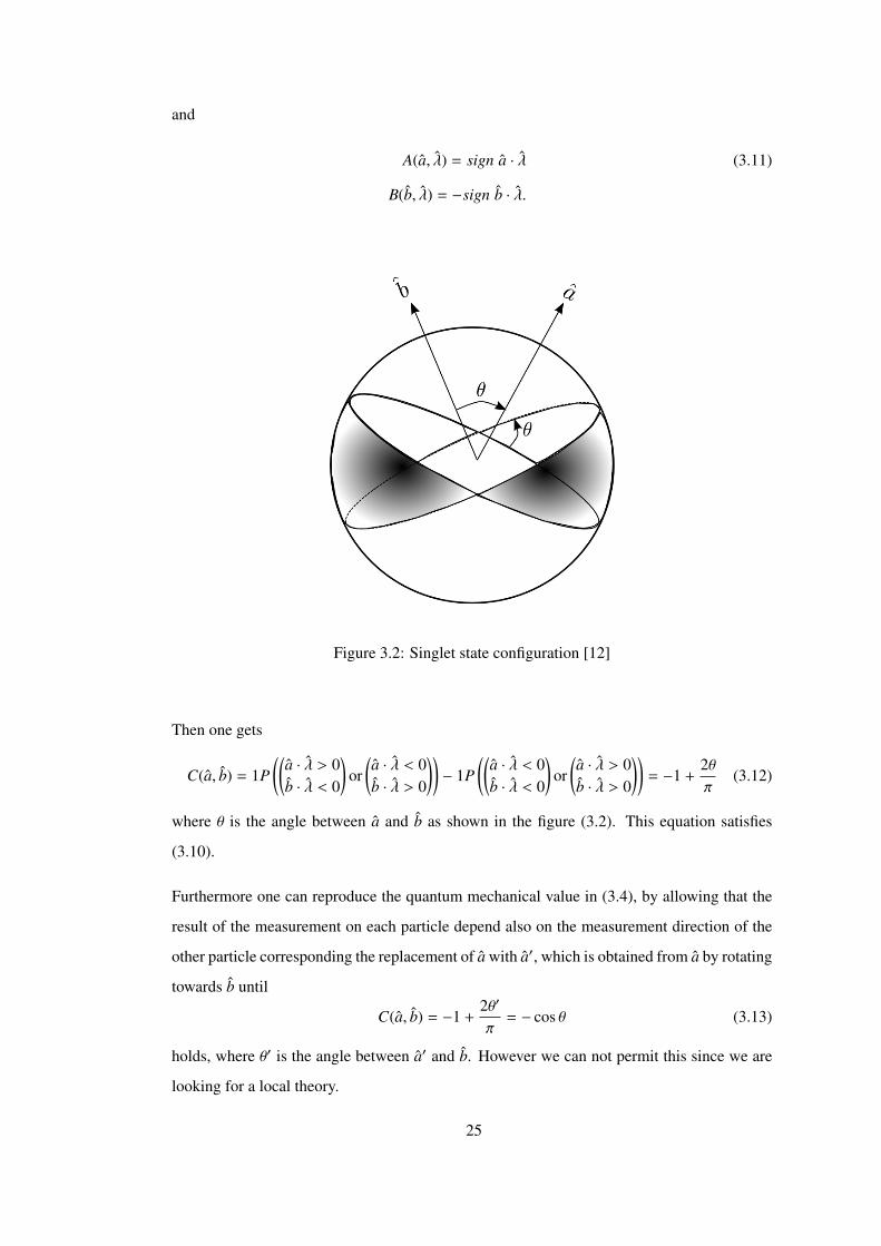
and
A(a, λ) = sign a · λ (3.11)
B(b, λ) = −sign b · λ.
Figure 3.2: Singlet state configuration [12]
Then one gets
C(a, b) = 1P((
a · λ > 0b · λ < 0
)or
(a · λ < 0b · λ > 0
))− 1P
((a · λ < 0b · λ < 0
)or
(a · λ > 0b · λ > 0
))= −1 +
2θπ
(3.12)
where θ is the angle between a and b as shown in the figure (3.2). This equation satisfies
(3.10).
Furthermore one can reproduce the quantum mechanical value in (3.4), by allowing that the
result of the measurement on each particle depend also on the measurement direction of the
other particle corresponding the replacement of a with a′, which is obtained from a by rotating
towards b until
C(a, b) = −1 +2θ′
π= − cos θ (3.13)
holds, where θ′ is the angle between a′ and b. However we can not permit this since we are
looking for a local theory.
25

Next we turn our attention to comparing the hidden variable theory and quantum mechanics.
To show the contradictions between the result of local hidden variable theory and the quantum
mechanics, we proceed as follows:
Since ρ is normalized, we have ∫dλρ(λ) = 1 (3.14)
and for the singlet state
A(a, λ) = −B(a, λ). (3.15)
Then (3.6) can be written as
C(a, b) = −
∫dλρ(λ)A(a, λ)A(b, λ). (3.16)
Next, we introduce another unit vector c, and consider
C(a, b) −C(a, c) = −
∫dλρ(λ)
(A(a, λ)A(b, λ) − A(a, λ)A(c, λ)
)(3.17)
=
∫dλρ(λ)A(a, λ)A(b, λ)
(A(b, λ)A(c, λ) − 1
)where we have used the fact that [A(b, λ)]2 = 1. Since A(a, λ) = ±1, this equation can be
written as
|C(a, b) −C(a, c)| ≤∫
dλρ(λ)(1 − A(b, λ)A(c, λ)
)(3.18)
then finally we get
1 + C(b, c) ≥ |C(a, b) −C(a, c)| (3.19)
This is the original form of famous Bell inequality. It is easy to show that for some special
Figure 3.3: Angles that violates the Bell inequality
directions this inequality can not be satisfied by the quantum mechanical result. The Bell
inequality (3.19) for the quantum mechanics becomes
1 − cos(θbc) ≥ | cos(θab) − cos(θac)|. (3.20)
26

One can easily see that this is not satisfied for the angles shown in figure (3.3).
As a result, introducing a variable to account for the measurement process does not correspond
to the right statistical behavior of quantum mechanics. However as in the case of (3.13), if
the measurement result of one of the entangled pair depends also on the measurement of the
other, then it meets the quantum mechanical criteria. Then this hidden variable must propagate
instantaneously, but such a theory can not be Lorentz invariant.
Thus, the question asked by EPR is solved by J. S. Bell and this solution has been verified by
A. Aspect in a series of experiments [13].
3.3 Definition of Entanglement
After the discussion on the two historically important papers, one can describe the entangle-
ment in terms of the postulates of quantum mechanics. According to Postulate 4, total Hilbert
space of the composite system is formed by tensor product of Hilbert spaces of subsystems.
In that total space, there are such states that can not be written as a tensor product of states
representing the subsystem.
Consider an n-partite composite system, and
|ψi〉 ∈ Hi where i = 1, 2, 3, · · · , n (3.21)
Then there are states in theH =⊗n
i=1Hi such that
|ψ〉 ,n⊗
i=1
|ψi〉. (3.22)
These states are called entangled states. Any state that is not entangled is called separable.
In this work, we only concentrate on bipartite states.
3.3.1 Bipartite Entanglement
Consider two quantum systems, the first one is owned by Alice, and the second one by Bob.
Alice’s system may be described by states in a Hilbert space HA of dimension N and Bob’s
oneHB of dimension M. The composite system of both parties is then described by the vectors
in the tensor-product form of the two spacesH = HA ⊗HB.
27

Let |ai〉 be a basis of Alice’s space and |b j〉 be basis of Bob’s space. Then in HA ⊗ HB we
have the set of all linear combinations of the states |ai〉 ⊗ |b j〉 to be used as bases. Thus any
state inHA ⊗HB can be written as
|ψ〉 =
N,M∑i, j=1
ci j|ai〉 ⊗ |b j〉 ∈ HA ⊗HB (3.23)
with a complex N × M matrix C = (ci j).
The measurement of observables can be defined in a similar way, if A is an observable on
Alice’s space and B on Bob’s space, the expectation value of A ⊗ B is defined as
〈ψ|(A ⊗ B)|ψ〉 =
N,M∑i, j=1
N,M∑i′, j′=1
c∗i jci′ j′〈ai|A|ai′〉〈b j|B|b j′〉. (3.24)
Now we can define separability and entanglement for these states. A pure state |ψ〉 ∈ H is
called a ”product state or separable” if one can find states |φA〉 ∈ HA and |φB〉 ∈ HB such that
|ψ〉 = |φA〉 ⊗ |φB〉 holds. Otherwise the state |ψ〉 is called entangled.
Physically, the definition of product state means that the state is uncorrelated. Thus a prod-
uct state can be prepared in a local way. In other word Alice produces the state |φA〉 and
Bob does independently |φB〉. If Alice measures any observable A and Bob measures B, the
measurement outcomes for Alice do not depend on the outcomes on Bob’s side.
In a pure state, it is easy to decide whether a given pure state is entangled or not. |ψ〉 is a
product state, if and only if the rank of the matrix C = (ci j) in (3.23) equals one. This is due
to the fact that a matrix C is of rank one, if and only if there exist two vectors a and b such
that ci j = aib j. So one can write
|ψ〉 =
∑i
ai|ai〉
⊗∑
j
b j|b j〉
(3.25)
which means that it is the product state. Another important tool for the description of en-
tanglement for bipartite systems only is the Schmidt decomposition, we turn our attention
next:
Let |ψ〉 =∑N,M
i, j=1 ci j|aib j〉 ∈ HA⊗HB be a vector in the tensor product space of the two Hilbert
spaces. Then there exists an orthonormal basis |i〉A of HA and an orthonormal basis |i〉B of
HB such that
|ψ〉 =
R∑i=1
λi|i〉A ⊗ |i〉B (3.26)
28
holds, with positive real coefficients λi. The λi’s are the square roots of eigenvalues of
matrix, CC† where C = (ci j), and are called the Schmidt coefficients. The number R =
min(dim(HA), dim(HB)) is called the Schmidt Rank/Number of |ψ〉. If R equals one then, the
state is product state, otherwise it is entangled. For an entangled state, if the absolute values
of all non vanishing Schmidt coefficients are the same, then it is called maximally entangled
state.
3.3.2 von Neumann Entropy
It is worth pointing out that from Schmidt form one can define the von Neumann entropy
which can be used as a measure of entanglement, as
S = −∑
j
|λ j|2 log2 |λ j|
2. (3.27)
From this definition, one can easily observe that if a given state is a product state which means
that the Schmidt rank is equal to one in the spectral decomposition, then the von Neumann
entropy is zero. However for an entangled state, the von Neumann entropy never vanishes.
Furthermore, for a maximally entangled state, the von Neumann entropy is
S = log2(R) (3.28)
where R > 1.
3.3.3 Bell States
An important set of entangled states are the Bell states, which are maximally entangled states.
|ψ+〉 =1√
2(|01〉 + |10〉) |φ+〉 =
1√
2(|00〉 + |11〉) (3.29)
|ψ−〉 =1√
2(|01〉 − |10〉) |φ−〉 =
1√
2(|00〉 − |11〉).
They form an orthonormal basis on the composite Hilbert space of bipartite system, in the
sense that any other state in this space can be produced from each of them by local operations.
Since the Bell states are already in the Schmidt form, one can find the von Neumann entropy
of these states by using (3.28) as
S = 1. (3.30)
29
3.4 CHSH Inequality
Bell inequality in (3.19) can be written in a more elegant way. For a bipartite system, consider
four dichotomous operators Q, R, S , and T which can take the values ±1. Let Q and R be
defined on the one system, S and T be on the other system, then with these four operator one
can write such an equation that
(Q + R)S + (Q − R)T = ±2 (3.31)
always holds. Average of this equation leads to an inequality
|〈(Q + R)S + (Q − R)T 〉| ≤ 2. (3.32)
It is the well known CHSH inequality [14]. This inequality states that any local theory must
satisfy it. However in quantum mechanics, expectation value of certain observables for the
entangled states violates this inequality as follows:
Consider the singlet state
|singlet〉 =1√
2(|s; ↑〉|s; ↓〉 − |s; ↓〉|s; ↑〉.) (3.33)
Since the singlet state is an entangled state in the spin degree of freedom, (3.32) can be written
in terms of correlation functions as
|C(a, b) + C(a′, b) + C(a′, b′) −C(a, b′)| ≤ 2 (3.34)
where a, b, a′, and b′ are the spin measurement directions. If one chooses the a, b, a′, and b′
as
a = (0, 0, 1)
b = (1/√
2, 0, 1/√
2)
a′ = (1, 0, 0)
b′ = (1/√
2, 0,−1/√
2)
then CHSH inequality for the singlet state gives
|C(a, b) + C(a′, b) + C(a′, b′) −C(a, b′)| = 2√
2. (3.35)
This is the verification of the non local character of quantum mechanics. CHSH inequality
is valid for the bipartite systems and any bipartite entangled state violates this inequality in
certain directions.
30

Furthermore one can find the upper limit of this inequality. Since these four operator are
dichotomous, square of these operators are equal to identity operator. As a result, one can
find
[(Q + R)S + (Q − R)T ]2 = 4I − [Q,R] ⊗ [S ,T ]. (3.36)
Then, taking the expectation value, and using the Schwarz’s Inequality, one can obtain
〈(Q + R)S + (Q − R)T 〉 ≤√
4 − 〈[Q,R] ⊗ [S ,T ]〉. (3.37)
This is the quantum generalization of Bell-type inequality [15]. One can find that upper
limit for the CHSH inequality is 2√
2. As a result, (3.35) is the maximum violation of the
inequality.
31

CHAPTER 4
LORENTZ TRANSFORMATION OF ENTANGLED STATES
AND BELL INEQUALITY
4.1 Transformation of Entangled States
In this thesis, we have only been interested in the transformation of the Bell states. Consider
a frame, S which observes the four momenta of the particles as p1 and p2, respectively. In
terms of the creation operators, these four states can be written in this frame as,
|Φ±〉 =1√
2
(a†(p1,
12
)a†(p2,12
) ± a†(p1,−12
)a†(p2,−12
))|0〉 (4.1)
|Ψ±〉 =1√
2
(a†(p1,
12
)a†(p2,−12
) ± a†(p1,−12
)a†(p2,12
))|0〉. (4.2)
For simplicity, it can be taken that these two particles identical and S frame can be chosen as
the zero momentum frame which means, p1 = −p2 = p = γβmz and also p01 = p0
2. Define
another frame S ′ which is boosted in the positive x direction relative to the S -frame.
We will now work out the transformation of these states to the frame S ′. First of all, we have
to determine the Wigner angles for both particles. For the first particle Ds=1/21 (θW) is given
by (2.82) and the Wigner angle, θW is in (2.79). For the second particle since L(p)−z in the
−z-direction, the Wigner rotation is about the +y-direction, but the angle is not changed, so
Ds=1/22 (θW) =
cos θW2 sin θW
2
− sin θW2 cos θW
2
. (4.3)
However transformed momenta are not the same. We will keep it as (Λ(−p)) and it is given
32
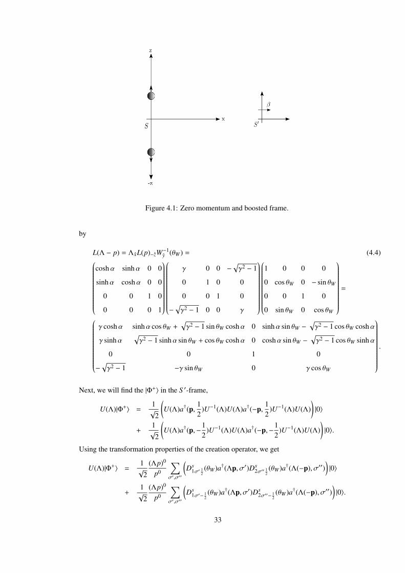
Figure 4.1: Zero momentum and boosted frame.
by
L(Λ − p) = ΛxL(p)−zW−1y (θW) = (4.4)
coshα sinhα 0 0
sinhα coshα 0 0
0 0 1 0
0 0 0 1
γ 0 0 −√γ2 − 1
0 1 0 0
0 0 1 0
−√γ2 − 1 0 0 γ
1 0 0 0
0 cos θW 0 − sin θW
0 0 1 0
0 sin θW 0 cos θW
=
γ coshα sinhα cos θW +√γ2 − 1 sin θW coshα 0 sinhα sin θW −
√γ2 − 1 cos θW coshα
γ sinhα√γ2 − 1 sinhα sin θW + cos θW coshα 0 coshα sin θW −
√γ2 − 1 cos θW sinhα
0 0 1 0
−√γ2 − 1 −γ sin θW 0 γ cos θW
.
Next, we will find the |Φ+〉 in the S ′-frame,
U(Λ)|Φ+〉 =1√
2
(U(Λ)a†(p,
12
)U−1(Λ)U(Λ)a†(−p,12
)U−1(Λ)U(Λ))|0〉
+1√
2
(U(Λ)a†(p,−
12
)U−1(Λ)U(Λ)a†(−p,−12
)U−1(Λ)U(Λ))|0〉.
Using the transformation properties of the creation operator, we get
U(Λ)|Φ+〉 =1√
2
(Λp)0
p0
∑σ′,σ′′
(Ds
1σ′ 12(θW)a†(Λp, σ′)Ds
2σ′′ 12(θW)a†(Λ(−p), σ′′)
)|0〉
+1√
2
(Λp)0
p0
∑σ′,σ′′
(Ds
1σ′− 12(θW)a†(Λp, σ′)Ds
2σ′′− 12(θW)a†(Λ(−p), σ′′)
)|0〉.
33

Now using the spin-s representation of rotations
U(Λ)|Φ+〉 =1√
2
(Λp)0
p0
(cos2 θW
2a†(Λp,
12
)a†(Λ(−p),12
) − cosθW
2sin
θW
2a†(Λp,
12
)a†(Λ(−p),−12
)
+ cosθW
2sin
θW
2a†(Λp,−
12
)a†(Λ(−p),12
) − sin2 θW
2a†(Λp,−
12
)a†(Λ(−p),−12
)
− sin2 θW
2a†(Λp,
12
)a†(Λ(−p),12
) − cosθW
2sin
θW
2a†(Λp,
12
)a†(Λ(−p),−12
)
+ cosθW
2sin
θW
2a†(Λp,−
12
)a†(Λ(−p),12
) + cos2 θW
2a†(Λp,−
12
)a†(Λ(−p),−12
))|0〉
one can obtain
U(Λ)|Φ+〉 =1√
2
(Λp)0
p0
(cos θWa†(Λp,
12
)a†(Λ(−p),12
) − sin θWa†(Λp,12
)a†(Λ(−p),−12
)
+ sin θWa†(Λp,−12
)a†(Λ(−p),12
) + cos θWa†(Λp,−12
)a†(Λ(−p),−12
))|0〉.
Finally, this can be written as
U(Λ)|Φ+〉 = cos θW |Φ+〉′ − sin θW |Ψ
−〉′. (4.5)
Similarly, one can find the transformation properties of the other Bell states as
U(Λ)|Φ−〉 = |Φ−〉′ (4.6)
U(Λ)|Ψ+〉 = |Ψ+〉′ (4.7)
U(Λ)|Ψ−〉 = sin θW |Φ+〉′ + cos θW |Ψ
−〉′ (4.8)
where θW = arctan(−γ′γβ′βγ′+γ ),
|Φ±〉′ =(Λp)0
p0
1√
2
(a†(Λp,
12
)a†(Λ(−p),12
) ± a†(Λp,−12
)a†(Λ(−p),−12
))|0〉 (4.9)
|Ψ±〉′ =(Λp)0
p0
1√
2
(a†(Λp,
12
)a†(Λ(−p),−12
) ± a†(Λp,−12
)a†(Λ(−p),12
))|0〉 (4.10)
and
Λ(±p) = m(−γ′γβ′ i ± βγk
),
(Λp)0
p0 = γ′. (4.11)
After these discussions it is obvious that entanglement is a Lorentz invariant property. No
inertial observer can see an entangled state as a product state.
This property can be proven in a general way starting from Schmidt form for bipartite states,
which is presented in the following section.
34

4.2 Schmidt Decomposition and Its Covariance
Consider two particles A and B. The total state vector of the composite system can be decom-
posed as
|ψ〉 =
R∑i=1
λi|i〉A ⊗ |i〉B (4.12)
where λi are the Schmidt coefficients, R = min(dim(HA), dim(HB)) is the Schmidt rank and
|i〉A and |i〉B are the orthonormal basis of the corresponding Hilbert spaces. These basis can
be normalized as
A〈i| j〉A = δ(p′A − pA)δi j (4.13)
B〈i| j〉B = δ(p′B − pB)δi j
where pA and pB momenta of the particles A and B, respectively. Therefore, the normalization
of the state vector of the composite system becomes
〈ψ|ψ〉 = δ(p′A − pA)δ(p′B − pB) (4.14)
with the condition∑
i |λi|2 = 1.
The orthonormal basis |i〉A and |i〉B can be expanded in terms of the single particle states as
the following
|i〉A =
sA∑n=−sA
A(i)n |pA, n〉 (4.15)
|i〉B =
sB∑m=−sB
B(i)m |pB,m〉
where sA and sB are the spins of the particles, respectively. As a result for this configuration,
R = min(sA, sB).
Since these basis should satisfy (4.13),
sA∑n=−sA
A∗( j)n A(i)
n δ(p′A − pA) = δ(p′A − pA)δi j (4.16)
sB∑m=−sB
B∗( j)m B(i)
m δ(p′B − pB) = δ(p′B − pB)δi j
must hold. Then, the Schmidt decomposition becomes
|ψ〉 =
R∑i=1
λi
sA∑n=−sA
sB∑m=−sB
A(i)n B(i)
m |pA, n〉 ⊗ |pB,m〉.
35

The single particle states can be written in terms of the creation operators as
|pA, n〉 = a†(pA, n)|0〉
|pB,m〉 = a†(pB,m)|0〉
where |0〉 is the Lorentz invariant vacuum state. Finally we get the Schmidt decomposition in
terms of the creation operators as
|ψ〉 =
R∑i=1
λi
sA∑n=−sA
sB∑m=−sB
A(i)n B(i)
m a†(pA, n)a†(pB,m)|0〉.
Now we can apply Lorentz transformation on our state ket by the unitary transformation U(Λ)
U(Λ)|ψ〉 =
R∑i=1
λi
sA∑n=−sA
sB∑m=−sB
A(i)n B(i)
m U(Λ)a†(pA, n)U−1(Λ)U(Λ)a†(pB,m)U−1(Λ)U(Λ)|0〉.
Using the transformation relations of the creation operators
U(Λ)a†(pA, n)U−1(Λ) =
√(ΛpA)0√(pA)0
sA∑n′=−sA
D(sA)n′n (WA)a†(ΛpA, n′)
U(Λ)a†(pB,m)U−1(Λ) =
√(ΛpB)0√(pB)0
sB∑m′=−sB
D(sB)m′m(WB)a†(ΛpB,m′)
and the Lorentz invariance of the vacuum, U(Λ)|0〉 = |0〉, we get
U(Λ)|ψ〉 =
R∑i=1
λi
sA∑n,n′=−sA
sB∑m,m′=−sB
A(i)n B(i)
m D(sA)n′n (WA)D(sB)
m′m(WB)
√(ΛpA)0√(pA)0
a†(ΛpA, n′)
√(ΛpB)0√(pB)0
a†(ΛpB,m′)|0〉
or
U(Λ)|ψ〉 =
R∑i=1
λi
sA∑n,n′=−sA
sB∑m,m′=−sB
A(i)n B(i)
m D(sA)n′n (WA)D(sB)
m′m(WB)|ΛpA, n′〉⊗|ΛpB,m′〉
√(ΛpA)0√(pA)0
√(ΛpB)0√(pB)0
.
Next we define
A(i)n′ =
sA∑n=−sA
D(sA)n′n (WA)A(i)
n
√(ΛpA)0√(pA)0
B(i)m′ =
sB∑m=−sB
D(sB)m′m(WB)B(i)
m
√(ΛpB)0√(pB)0
.
Then, the transformed state becomes
U(Λ)|ψ〉 =
R∑i=1
λi
sA∑n′=−sA
sB∑m′=−sB
A(i)n′ B
(i)m′ |ΛpA, n′〉 ⊗ |ΛpB,m′〉.
This expression can be re-written as
U(Λ)|ψ〉 = |ψ〉 =
R∑i=1
λi|i〉A ⊗ |i〉B
36
where
|i〉A =
sA∑n′=−sA
A(i)n′ |ΛpA, n′〉 =
sA∑n′=−sA
sA∑n=−sA
D(sA)n′n (WA)A(i)
n |ΛpA, n′〉
√(ΛpA)0√(pA)0
|i〉B =
sB∑m′=−sB
B(i)m′ |ΛpB,m′〉 =
sB∑m′=−sB
sB∑m=−sB
D(sB)m′m(WB)B(i)
m |ΛpB,m′〉
√(ΛpB)0√(pB)0
.
It is necessary now to check whether {|i〉} forms an orthonormal basis. For this, consider
A〈i| j〉A =
sA∑n′′=−sA
sA∑n′=−sA
A∗(i)n′′ A( j)n′ 〈Λp′A, n
′′|ΛpA, n′〉︸ ︷︷ ︸δn′n′′δ(Λp′A−ΛpA)=δn′n′′
(pA)0
(ΛpA)0δ(p′A−pA)
=
sA∑n′=−sA
A∗(i)n′ A( j)n′
(pA)0
(ΛpA)0 δ(p′A − pA)
=
sA∑n′=−sA
sA∑m=−sA
A∗(i)m D∗(sA)mn′ (WA)
sA∑m′=−sA
D(sA)n′m′(WA)A( j)
m′δ(p′A − pA)
=
sA∑m,m′=−sA
A∗(i)m A( j)m′δ(p
′A − pA)
sA∑n′=−sA
D∗(sA)mn′ (WA)D(sA)
n′m′(WA)︸ ︷︷ ︸δmm′
=
sA∑m=−sA
A∗(i)m A( j)m δ(p′A − pA). (4.17)
Using (4.16), we get 〈i| j〉 = δi jδ(p′A−pA). This means that the transformed state is still in the
Schmidt decomposition form with exactly the same Schmidt coefficients. This result proves
the Lorentz covariance of entanglement.
Also note that since the Schmidt coefficients do not change under Lorentz transformation, the
Von Nuemann entropy as a measure of entanglement do not increase or decrease, since
S = −∑
s
|λs|2 log2 |λs|
2. (4.18)
Therefore, the von Neumann entropy is a Lorentz invariant quantity. To illustrate the invari-
ance, consider the transformed state (4.5), it can be written in the Schmidt form as,
U(Λ)|Φ+〉 =
1√
2
{cos(θW)
√(Λp)0
p0 a†(Λp,12
) + sin(θW)
√(Λp)0
p0 a†(Λp,−12
)}⊗
√(Λp)0
p0 a†(Λ(−p),12
)
+1√
2
{cos(θW)
√(Λp)0
p0 a†(Λp,−12
) − sin(θW)
√(Λp)0
p0 a†(Λp,12
)}⊗
√(Λp)0
p0 a†(Λ(−p),−12
)
37
where the bases satisfies (4.16). Then the von Neumann entropy is
S = −
(12
log2(12
) +12
log2(12
))
= 1
which is agree with (3.30).
4.3 Correlation Function and Bell Inequality
Now we turn our attention to the calculation of the correlation function
C(a, b) = 〈SN1 · a,S
N2 · b〉 (4.19)
for the state (4.8). There is an easy way of calculating this correlation function by using the
properties of entangled states, which is
S 1Ni |Φ
+〉′ = S 2Ni |Φ
+〉′ (4.20)
S 1Ni |Ψ
−〉′ = −S 2Ni |Ψ
−〉′.
Then, the correlation function becomes
C(a, b) =
(cos θW〈Ψ
−|′ + sin θW〈Φ+|′
)SN
1 · a SN2 · b
(cos θW |Ψ
−〉′ + sin θW |Φ+〉′
)=
(cos2 θW〈Ψ
−|′S 1Ni aiS 2
Nj b j|Ψ
−〉′ + sin2 θW〈Φ+|′S 1
Ni aiS 2
Nj b j|Φ
+〉′)
+ cos θW sin θW(〈Ψ−|′S 1
Ni aiS 2
Nj b j|Φ
+〉′ + 〈Φ+|′S 1Ni aiS 2
Nj b j|Ψ
−〉′)
= − cos2 θW〈Ψ−|′S 1
Ni aiS 1
Nj b j|Ψ
−〉′ + sin2 θW〈Φ+|′S 1
Ni aiS 1
Nj b j|Φ
+〉′
+ cos θW sin θW(〈Ψ−|′S 1
Ni aiS 1
Nj b j|Φ
+〉′ − 〈Φ+|′S 1Ni aiS 1
Nj b j|Ψ
−〉′)
and using ( 2.46) we get
C(a, b) = aib j
(− cos2 θW〈Ψ
−|′(δi j + iεi jkS 1Nk )|Ψ−〉′ + sin2 θW〈Φ
+|′(δi j + iεi jkS 1Nk )|Φ+〉′
)+ aib j
(cos θW sin θW
(〈Ψ−|′(δi j + iεi jkS 1
Nk )|Φ+〉′ − 〈Φ+|′(δi j + iεi jkS 1
Nk )|Ψ−〉′
) )After carrying out the algebra, this reduces to
C(a, b) = −a · b cos(2θW) +i2
sin(2θW)(a × b) ·(〈Ψ−|′SN
1 |Φ+〉′ − 〈Φ+|′SN
1 |Ψ−〉′
). (4.21)
It can be re-written as
C(a, b) = −a · b cos(2θW) − (a × b) · =(〈Ψ−|′SN
1 |Φ+〉′
)sin(2θW). (4.22)
38

Figure 4.2: CHSH values versus velocity of the particles and the boosted frame, β and β′,respectively.
Now we are ready to test the locality condition by using CHSH inequality
CHS H = C(a, b) + C(a′, b) + C(a′, b′) −C(a, b′). (4.23)
One can choose the measurement directions as the following
a = (1/√
2,−1/√
2, 0)
a′ = (−1/√
2,−1/√
2, 0) (4.24)
b = (0, 1, 0)
b′ = (1, 0, 0)
39

corresponding to the case that they give maximum violation in the non relativistic limit. Then
one obtains the result of the CHS H as
CHS H = 2√
2 cos(2θW). (4.25)
Using (2.79), this result can be defined in terms of the particle velocity β and the velocity of
the boosted frame β′, as
CHS H = 2√
2
1 − β2 + 1 − β′2 + 2√
1 − β2√
1 − β′2 − β2β′2
1 − β2 + 1 − β′2 + 2√
1 − β2√
1 − β′2 + β2β′2
. (4.26)
From these two equivalent results, it can be deduced that in the non relativistic domain, β and
β′ → 0 as shown in the figure (4.2), there is no Wigner rotation, so it gives the maximum
violation. Again if the boost direction is parallel or anti-parallel to the direction of the particle
as seen by the zero momentum frame, then there is no rotation and we get the maximum vio-
lation as in [16]. However in the ultra relativistic limit β, β′ → 1, we again get the maximum
violation as in the [16], contrary to that of [17].
Actually, it is an illusion that the CHS H inequality is satisfied for certain values of β and
β′. Since the Wigner rotation that increases with the increased velocity changes the spin
polarization direction as observed from the zero momentum frame, it is natural that initial Bell
observables, (4.24) may satisfy the CHS H inequality at certain velocities. As a result one can
still find some directions that violates the CHS H inequality for the mentioned velocities that
satisfies the inequality for the initial directions (4.24). For example, when θW = π4 , (4.25) is
zero, so CHS H inequality is satisfied. However at this Wigner angle, if one re-defines the
measurement directions as the follows,
a = (0, 0, 1)
a′ = (1, 0, 0)
b = (−1/√
2, 0,−1/√
2)
b′ = (1/√
2, 0, 1/√
2)
then, the correlation function (4.22) turns into
C(a, b) = −(a × b) · =(〈Ψ−|′SN
1 |Φ+〉′
)(4.27)
and it is found that
CHS H = −2√
2. (4.28)
40

The resolution of this illusion can be done by introducing the Wigner angle dependent di-
chotomous operators. In other words, it is necessary to choose these operators by taking
into consideration the Wigner angle. Thus, one can always show that transformed state still
violates the Bell type inequalities in certain directions.
41
CHAPTER 5
CONCLUSION
In this thesis, we have investigated the entanglement problem in the context of relativistic
quantum mechanics. Entanglement lies at the heart of the quantum mechanics due to its non
local character. In this sense, studying its properties in the framework of special relativity
is crucial. For this purpose, we have first constructed the unitary irreducible representation
of Poincare group in the infinite dimensional Hilbert space. In this framework, the issue of
finding the unitary irreducible representations of Poincare group is reduced to that of the little
group. Namely in this formalism Poincare group reduces to the three dimensional rotation
group for the massive cases, entangled states in different but equivalent frames undergo a
Wigner rotation which changes its spin polarization direction.
On the other hand, since there are some ambiguities on the correct relativistic operator in the
literature, we have critically studied physical requirements on it. Spin statistics must be a
frame-independent property, and therefore square of the correct three-spin operator should be
a Lorentz invariant as implied by the second Casimir operator of Poincare group.
Specifically, we have analyzed the Bell states under Lorentz transformations. Although these
entangled states can mix, we have shown that the entanglement is a Lorentz invariant phenom-
ena. This invariance has been shown for any entangled bipartite system by starting from the
Schmidt decomposition. Then we have calculated the correlation function for the transformed
states. Using the correlation, we have constructed the CHS H inequality. At the first glance
, CHS H inequality seems to be satisfied for certain Wigner angles that depends on both the
velocity of the particle and velocity of the boosted frame relative to the zero momentum frame
of the entangled state. However, it is an illusion since changes in the velocities cause changes
in the Wigner angle that can affect the superposition of the entangled states which violate
42
the CHS H inequality in different directions. Thus, it is natural that the initial dichotomous
operators may satisfy the inequality for these entangled states. This confusing situation can
be solved radically by performing the EPR experiment with the Wigner angle dependent di-
chotomous operators. As a result, Lorentz transformed entangled states still violates the Bell
type inequalities in certain directions that may depend on the Wigner angle.
43

REFERENCES
[1] A. Einstein, B. Podolsky, and N. Rosen, Phys. Rev. 47, 777 (1935).
[2] E. Schrodinger, Die gegenwartige Situation in der Quantenmechanik, Naturwis-senschaften 23, 807; 23 823; 23 844 (1935); English translation by J. D. Trimmer, ThePresent Situation in Quantum Mechanics: A Translation of Schrodinger’s “Cat Paradox”Paper, Proceedings of the American Philosophical Society 124, 323 (1980).
[3] R. Horodecki, P. Horodecki, M. Horodecki, and K. Horodecki, Rev. Mod. Phys. 81, 2(2009).
[4] J. S. Bell, Physics 1, 195 (1964).
[5] P. M. Alsing and G. J. Milburn, Lorentz Invariance of Entanglement, arXiv:quant-ph/0203051v1
[6] S. Weinberg, The Quantum Theory of Fields I, (Cambridge University Press, N.Y. 1995).
[7] E. P. Wigner, Gruppentheorie und ihre Anwendung auf die Quantenmechanik der Atom-spekten, (Braunschweig, 1931; English translation, Academic Press, Inc, New York,1959).
[8] W. I. Fushchich, A. G. Nikitin, Symmetries of Equations of Quantum Mechanics, (NewYork, 1994).
[9] E.V. Stefanovich, Relativistic Quantum Dynamics, preprint arxiv:physics/0504062
[10] E. P. Wigner, Ann. Math. 40, 149 (1939).
[11] D. Bohm and Y. Aharonov, Phys. Rev. 108, 1070 (1957).
[12] A. Peres, Quantum Theory: Concepts and Methods (Kluwer, Dordrecht, 1993).
[13] A. Aspect, P. Grangier, and G. Roger, Phys. Rev. Lett. 47, 460 (1981); A. Aspect, J.Dalibard, and G. Roger, Phys. Rev. Lett. 49, 1804 (1982); A. Aspect, P. Grangier, andG. Roger, Phys. Rev. Lett. 49, 91 (1982).
[14] J. F. Clauser, M.A. Horne, A. Shimony and R. A. Holt, Phys. Rev. Lett. 23, 880-884(1969).
[15] B. S. Cirel’son, Lett. Math. Phys. 4, 93 (1980).
[16] P. Caban and J. Rembielin’ski, Phys. Rev. A 74, 042103 (2006).
[17] D. Ahn, H. J. Lee, Y. H. Moon, and S. W. Hwang, Phys. Rev. A 67, 012103 (2003).
44