EN/SUT/2014/Doc/1 - ECAStats: Online accessecastats.uneca.org/acsweb/Portals/0/Economic Statistics... · Web view2369 6678 804 5707 913 1867 967 8324 15002 5. TLS-prod 33 177 123

EN/SUT/2014/Doc/14

Chapter 13: Supply and use tables and input-output tables

13.1. Introduction1. This chapter provides the sequence of steps that are required to convert SUTs to Input-

Output (I-O) tables and use of I-O tables for economic analysis. The chapter also

presents simplified procedures for preparing I-O tables, I-O models and for carrying out

economic analysis with an example of a three-sector economy.

2. The input-output framework comprises, (i) supply table at basic prices with

transformation to purchasers’ prices, (ii) use table at purchasers’ prices, which is

subsequently transformed to basic prices, and (iii) symmetric I-O tables, which are built

up from the SUTs at basic prices. While the supply and use tables (SUTs) are product

by industry tables, the I-O tables are either product by product or industry by industry

tables. Both the SUTs and I-O tables provide the inter-industry dependencies and

relationship between producers and consumers. They, thus offer a most detailed picture

of the economy, which essentially involves (a) production - industries producing

products in the form of goods and services, (b) consumption – both intermediate

(purchases of goods and services by industries) and final (purchases of goods and

services by domestic final users comprising households, non-profit institutions serving

households (NPISHs) and general government (all levels of Government in the

economy)), (c) accumulation that involves gross fixed capital formation (GFCF) and

change in inventories, and (d) transactions with the rest of the world (exports and

imports).

3. SUTs are the basis for the construction of symmetric I-O tables. I-O tables cannot be

compiled without passing through the supply and use stage. Symmetric I-O tables are

the basis for input-output analysis. While SUTs are close to statistical sources and actual

observations, I-O tables serve in a better way analytical purposes for economic analysis.

4. The I-O table is derived from the use table at purchasers’ prices, which, as mentioned

earlier, is a product by industry table. The use table constructed is often rectangular

with more products than industries in general. However, for the I-O table, rows and

columns should both have either products or industries with individual row totals and

columns totals to be equal, which necessitates that the I-O tables are square and

symmetric. A simple three sector square SUTs at purchasers’ prices are presented in the

following two tables. These tables have been used in this chapter to demonstrate the

preparation of I-O tables and economic analysis.

13.2. Conversion of SUTs at purchasers’ prices to I-O tables

5. The various steps involved in transforming the SUTs at purchasers’ prices to I-O tables

at basic prices are:

(i) Making SUTs square1: Transformation of rectangular SUTs at purchasers prices to

square SUTs at purchasers’ prices, with products in rows representing the

characteristic products of industries shown in columns;

(ii) Converting the square SUTs at purchasers’ prices to square SUTs at basic prices;

(iii) Application of standard models for transformation of square SUTs at basic prices

to product by product or industry by industry symmetric I-O tables2.

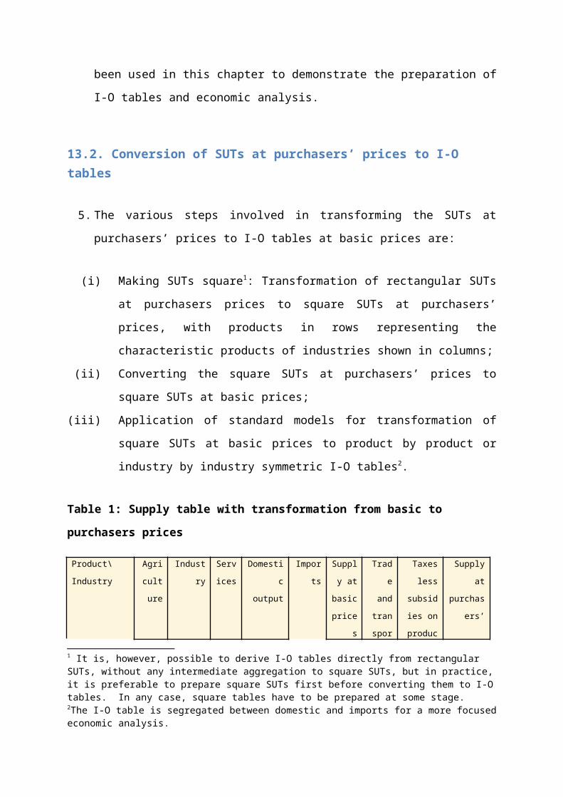
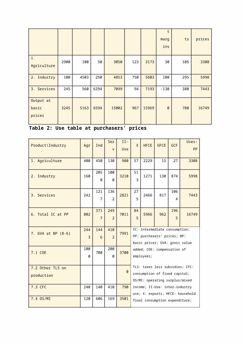
Table 1: Supply table with transformation from basic to purchasers prices

Product\IndustryAgric

ultureIndustry

Servi

ces

Domestic

outputImports

Supply

at basic

prices

Trade

and

transp

ort

margin

s

Taxes

less

subsidies

on

products

Supply at

purchasers

’ prices

1. Agriculture 2900 100 50 3050 123 3173 30 105 3308

2. Industry 100 4503 250 4853 750 5603 100 295 5998

1 It is, however, possible to derive I-O tables directly from rectangular SUTs, without any intermediate aggregation to square SUTs, but in practice, it is preferable to prepare square SUTs first before converting them to I-O tables. In any case, square tables have to be prepared at some stage.2The I-O table is segregated between domestic and imports for a more focused economic analysis.

3. Services 245 560 6294 7099 94 7193 -130 380 7443

Output at basic

prices3245 5163 6594 15002 967 15969 0 780 16749

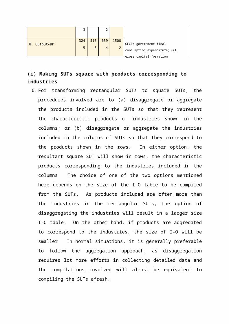
Table 2: Use table at purchasers’ prices

Product\Industry Agr Ind Serv II-Use X HFCE GFCE GCF Uses- PP

1. Agriculture 400 450 130 980 57 2229 15 27 3308

2. Industry 160 2050 1000 321051

31271 130 874 5998

3. Services 242 1217 1362 282127

52466 817 1064 7443

6. Total IC at PP 802 3717 2492 701184

55966 962 1965 16749

7. GVA at BP (8-6) 2443 1446 4102 7991 IC: intermediate consumption; PP: purchasers’

prices; BP: basic prices; GVA: gross value

added; COE: compensation of employees;

TLS: taxes less subsidies; CFC: consumption of

fixed capital; OS/MI: operating surplus/mixed

income; II-Use: inter-industry use; X: exports,

HFCE: household final consumption

expenditure; GFCE: government final

consumption expenditure; GCF: gross capital

formation

7.1 COE 1000 700 2000 3700

7.2 Other TLS on production 0

7.3 CFC 240 140 410 790

7.4 OS/MI 1203 606 1692 3501

8. Output-BP 3245 5163 6594 15002

(i) Making SUTs square with products corresponding to industries

6. For transforming rectangular SUTs to square SUTs, the procedures involved are to (a)

disaggregate or aggregate the products included in the SUTs so that they represent the

characteristic products of industries shown in the columns; or (b) disaggregate or

aggregate the industries included in the columns of SUTs so that they correspond to the

products shown in the rows. In either option, the resultant square SUT will show in

rows, the characteristic products corresponding to the industries included in the

columns. The choice of one of the two options mentioned here depends on the size of

the I-O table to be compiled from the SUTs. As products included are often more than

the industries in the rectangular SUTs, the option of disaggregating the industries will

result in a larger size I-O table. On the other hand, if products are aggregated to

correspond to the industries, the size of I-O will be smaller. In normal situations, it is

generally preferable to follow the aggregation approach, as disaggregation requires lot

more efforts in collecting detailed data and the compilations involved will almost be

equivalent to compiling the SUTs afresh.

7. For classifying industries in the SUTs, SNA recommends the use of International

Standard Industrial Classification (ISIC) for industries and Central Product

Classification (CPC) for products. Since the SUTs use the ISIC and CPC classifications

or country-specific classifications based on ISIC and CPC, it is possible to align the

products with industries in the SUTs, based on standard concordance tables available in

the UNSD website. Using these concordance tables, the square SUTs at purchasers’

prices can be prepared from the rectangular SUTs at purchasers’ prices, in which the

industry classification and the product classification are fully aligned with each other,

industries and products correspond to each other and the number of industries and the

number of products are the same.

(ii) Conversion of SUTs at purchasers’ prices to SUTs at basic prices

8. The next step involved in the long process of converting rectangular SUTs at

purchasers’ prices to symmetric I-O tables, is the transformation of square SUTs at

purchasers’ prices to square SUTs at basic prices3. For this purpose, it is necessary to

bring both the supply and the use tables to basic price valuations. It may be recalled

that the rectangular supply table at basic prices, initially compiled is already at basic

prices, as domestic output and imports, c.i.f. are at basic prices. Therefore, supply table

at basic prices is an integral part of the supply table at purchasers’ prices, since this

table includes a transformation of products from basic prices to purchasers’ prices by

adding the vectors of trade and transport margins (TTM), and taxes less subsidies (TLS)

on products. Thus, the square supply table at basic prices is readily available from the

square supply table at purchasers’ prices.

3It should be noted here that the intermediate and final uses calculated at basic prices are one step further removed from basic statistics and actual observations.

9. Thus, the task remains is only to compile a square use table at basic prices4 from the

square SUTs at purchasers’ prices. The cell values corresponding to the products

(quadrant I and quadrant II) in the use table at purchasers’ prices include values at basic

prices, trade margins, transport costs and taxes less subsidies on products in an

integrated manner. For the use table at basic prices, each of these components need to

be segregated from these cell values and placed in the respective rows of trade, transport

and taxes less subsidies on products. While the trade and transport rows already existing

in the use table will now include the total values segregated from the corresponding

cells in the same columns, a separate row needs to be introduced for taxes less subsidies

on products at the end of the product rows, as intermediate consumption of industries

would still need to be valued at purchasers’ prices.

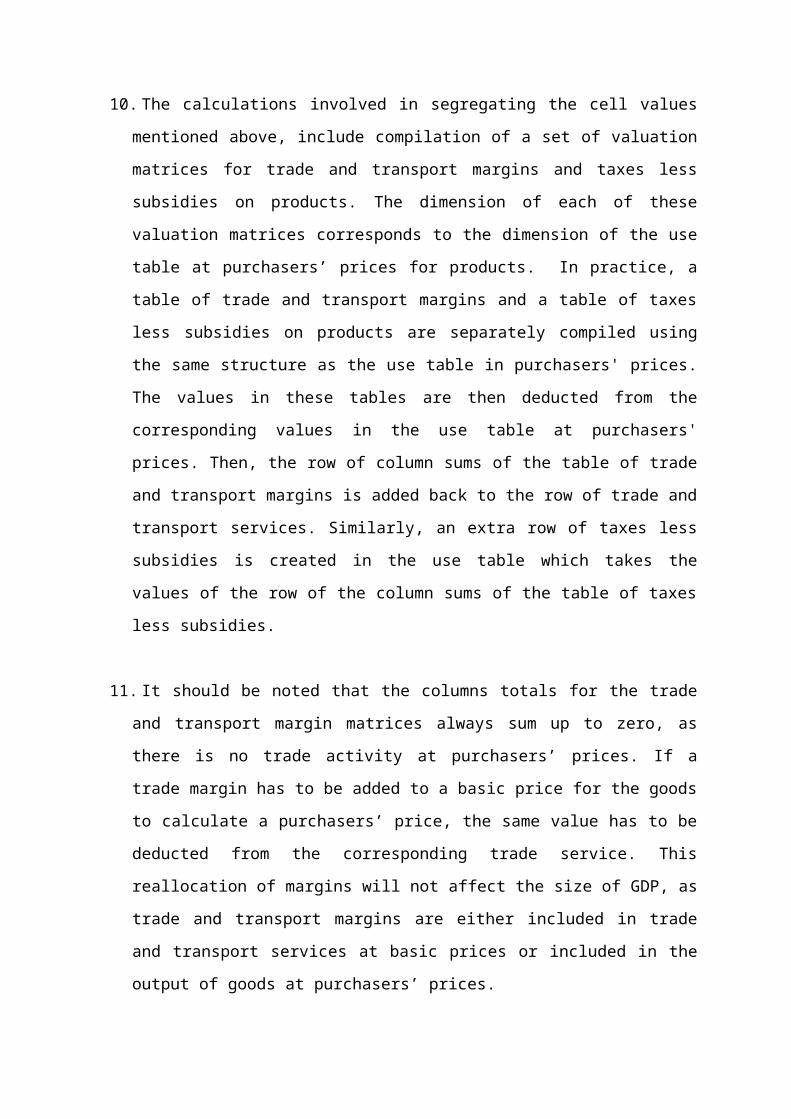
10. The calculations involved in segregating the cell values mentioned above, include

compilation of a set of valuation matrices for trade and transport margins and taxes less

subsidies on products. The dimension of each of these valuation matrices corresponds to

the dimension of the use table at purchasers’ prices for products. In practice, a table of

trade and transport margins and a table of taxes less subsidies on products are separately

compiled using the same structure as the use table in purchasers' prices. The values in

these tables are then deducted from the corresponding values in the use table at

purchasers' prices. Then, the row of column sums of the table of trade and transport

margins is added back to the row of trade and transport services. Similarly, an extra row

of taxes less subsidies is created in the use table which takes the values of the row of the

column sums of the table of taxes less subsidies.

11. It should be noted that the columns totals for the trade and transport margin matrices

always sum up to zero, as there is no trade activity at purchasers’ prices. If a trade

margin has to be added to a basic price for the goods to calculate a purchasers’ price, the

same value has to be deducted from the corresponding trade service. This reallocation of

margins will not affect the size of GDP, as trade and transport margins are either

included in trade and transport services at basic prices or included in the output of goods

at purchasers’ prices.

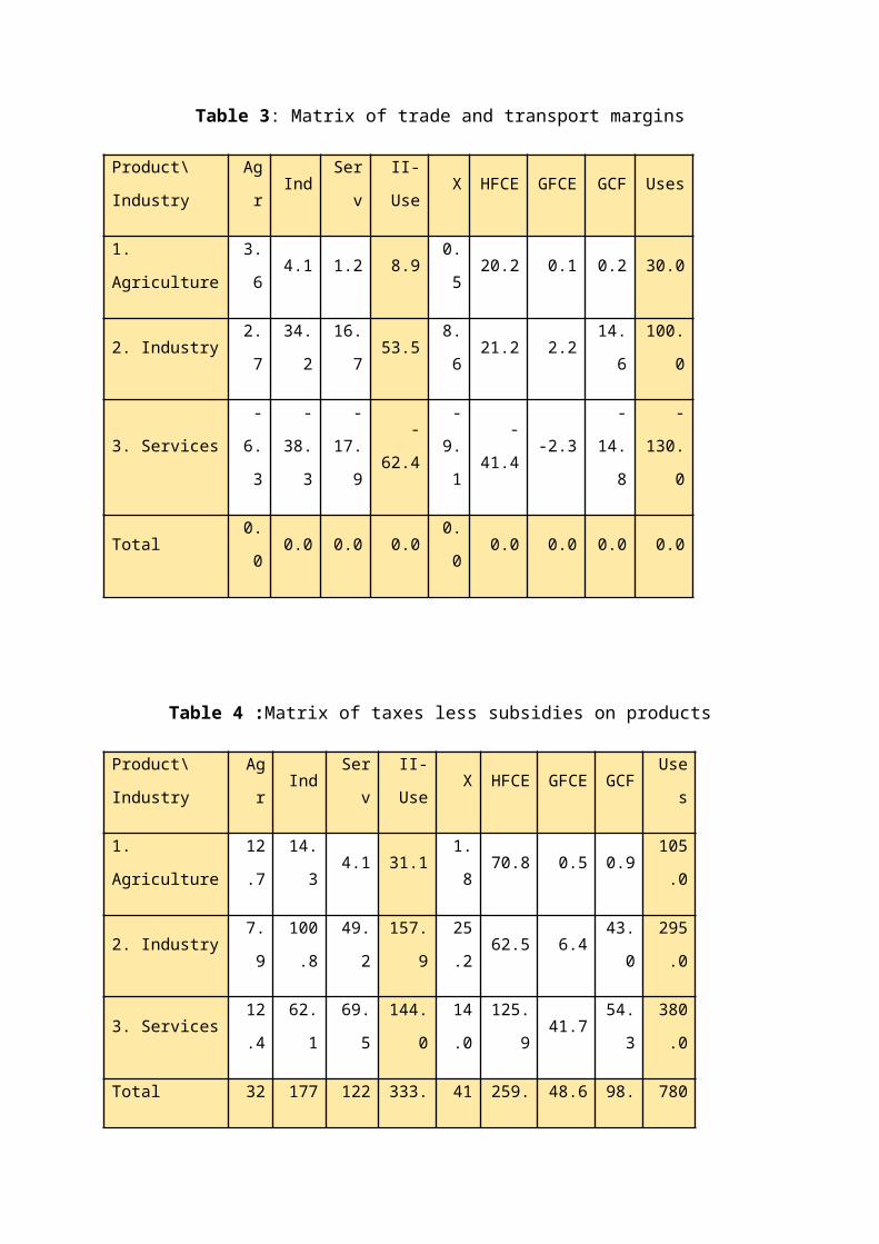
Table 3: Matrix of trade and transport margins

4The use tables at basic prices is defined as use table at purchasers' prices less trade margins, transport margins and net taxes on products.

Product\

IndustryAgr Ind Serv

II-

UseX HFCE GFCE GCF Uses

1. Agriculture 3.6 4.1 1.2 8.9 0.5 20.2 0.1 0.2 30.0

2. Industry 2.7 34.2 16.7 53.5 8.6 21.2 2.2 14.6 100.0

3. Services -6.3 -38.3 -17.9 -62.4 -9.1 -41.4 -2.3 -14.8 -130.0

Total 0.0 0.0 0.0 0.0 0.0 0.0 0.0 0.0 0.0

Table 4 :Matrix of taxes less subsidies on products

Product\


II-


1. Agriculture 12.7 14.3 4.1 31.1 1.8 70.8 0.5 0.9 105.0

2. Industry 7.9 100.8 49.2 157.925.

262.5 6.4 43.0 295.0

3. Services 12.4 62.1 69.5 144.014.

0125.9 41.7 54.3 380.0

Total 32.9 177.2 122.8 333.041.

1259.2 48.6 98.2 780.0

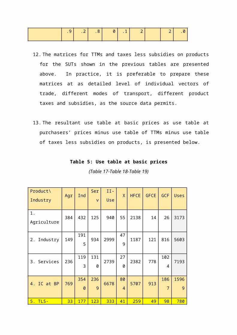
12. The matrices for TTMs and taxes less subsidies on products for the SUTs shown in the

previous tables are presented above. In practice, it is preferable to prepare these

matrices at as detailed level of individual vectors of trade, different modes of transport,

different product taxes and subsidies, as the source data permits.

13. The resultant use table at basic prices as use table at purchasers’ prices minus use table

of TTMs minus use table of taxes less subsidies on products, is presented below.

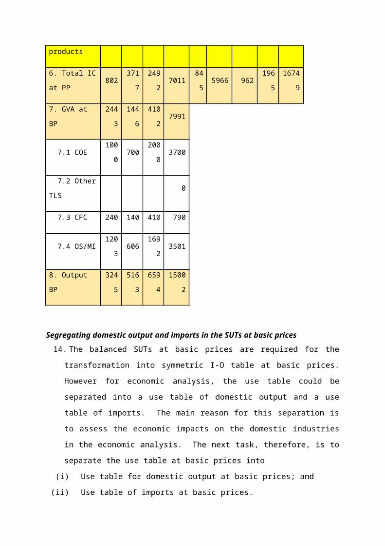
Table 5: Use table at basic prices

(Table 17-Table 18-Table 19)

Product\


II-


1. Agriculture 384 432 125 940 55 2138 14 26 3173

2. Industry 149191

5934 2999 479 1187 121 816 5603

3. Services 236119

31310 2739 270 2382 778 1024 7193

4. IC at BP 769354

02369 6678 804 5707 913 1867 15969

5. TLS-products 33 177 123 333 41 259 49 98 780

6. Total IC at PP 802371

72492 7011 845 5966 962 1965 16749

7. GVA at BP 2443144

64102 7991

7.1 COE 1000 700 2000 3700

7.2 Other TLS 0

7.3 CFC 240 140 410 790

7.4 OS/MI 1203 606 1692 3501

8. Output BP 3245516

36594 15002

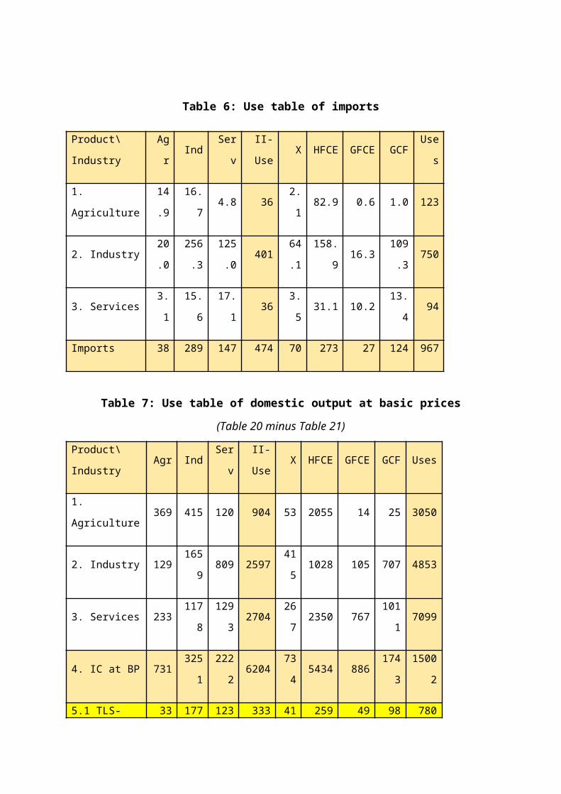
Segregating domestic output and imports in the SUTs at basic prices14. The balanced SUTs at basic prices are required for the transformation into symmetric I-

O table at basic prices. However for economic analysis, the use table could be separated

into a use table of domestic output and a use table of imports. The main reason for this

separation is to assess the economic impacts on the domestic industries in the economic

analysis. The next task, therefore, is to separate the use table at basic prices into

(i) Use table for domestic output at basic prices; and

(ii) Use table of imports at basic prices.

Table 6: Use table of imports

Product\


II-


1. Agriculture 14.9 16.7 4.8 36 2.1 82.9 0.6 1.0 123

2. Industry 20.0 256.3 125.0 40164.

1158.9 16.3 109.3 750

3. Services 3.1 15.6 17.1 36 3.5 31.1 10.2 13.4 94

Imports 38 289 147 474 70 273 27 124 967

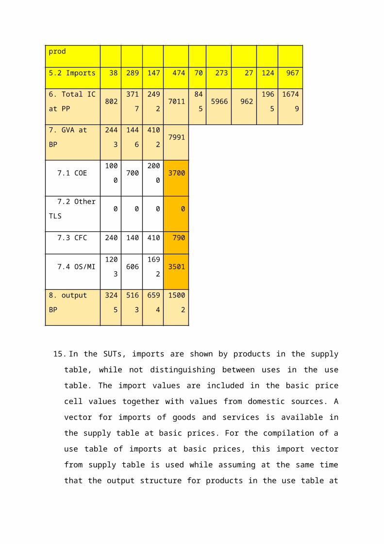
Table 7: Use table of domestic output at basic prices

(Table 20 minus Table 21)

Product\


II-


1. Agriculture 369 415 120 904 53 2055 14 25 3050

2. Industry 129165

9809 2597 415 1028 105 707 4853

3. Services 233117

81293 2704 267 2350 767 1011 7099

4. IC at BP 731325

12222 6204 734 5434 886 1743 15002

5.1 TLS-prod 33 177 123 333 41 259 49 98 780

5.2 Imports 38 289 147 474 70 273 27 124 967


72492 7011 845 5966 962 1965 16749

7. GVA at BP 2443144

64102 7991

7.1 COE 1000 700 2000 3700

7.2 Other TLS 0 0 0 0

7.3 CFC 240 140 410 790

7.4 OS/MI 1203 606 1692 3501

8. output BP 3245516

36594 15002

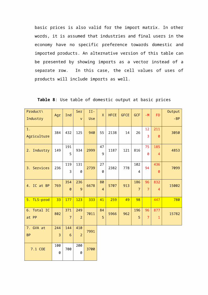
15. In the SUTs, imports are shown by products in the supply table, while not

distinguishing between uses in the use table. The import values are included in the basic

price cell values together with values from domestic sources. A vector for imports of

goods and services is available in the supply table at basic prices. For the compilation of

a use table of imports at basic prices, this import vector from supply table is used while

assuming at the same time that the output structure for products in the use table at basic

prices is also valid for the import matrix. In other words, it is assumed that industries

and final users in the economy have no specific preference towards domestic and

imported products. An alternative version of this table can be presented by showing

imports as a vector instead of a separate row. In this case, the cell values of uses of

products will include imports as well.

Table 8: Use table of domestic output at basic prices

Product\Industry Agr Ind ServII-

UseX HFCE GFCE GCF -M FD Output -BP

1. Agriculture 384 432 125 940 55 2138 14 26 123 2110 3050

2. Industry 149 191 934 2999 479 1187 121 816 750 1854 4853

5

3. Services 236119

31310 2739 270 2382 778

102

494 4360 7099

4. IC at BP 769354

02369 6678 804 5707 913

186

7967 8324 15002

5. TLS-prod 33 177 123 333 41 259 49 98 447 780


72492 7011 845 5966 962

196

5967 8771 15782

7. GVA at BP 2443144

64102 7991

7.1 COE 1000 700 2000 3700

7.2 Other TLS 0 0 0 0

7.3 CFC 240 140 410 790

7.4 OS/MI 1203 606 1692 3501

8. Output BP 3245516

36594 15002

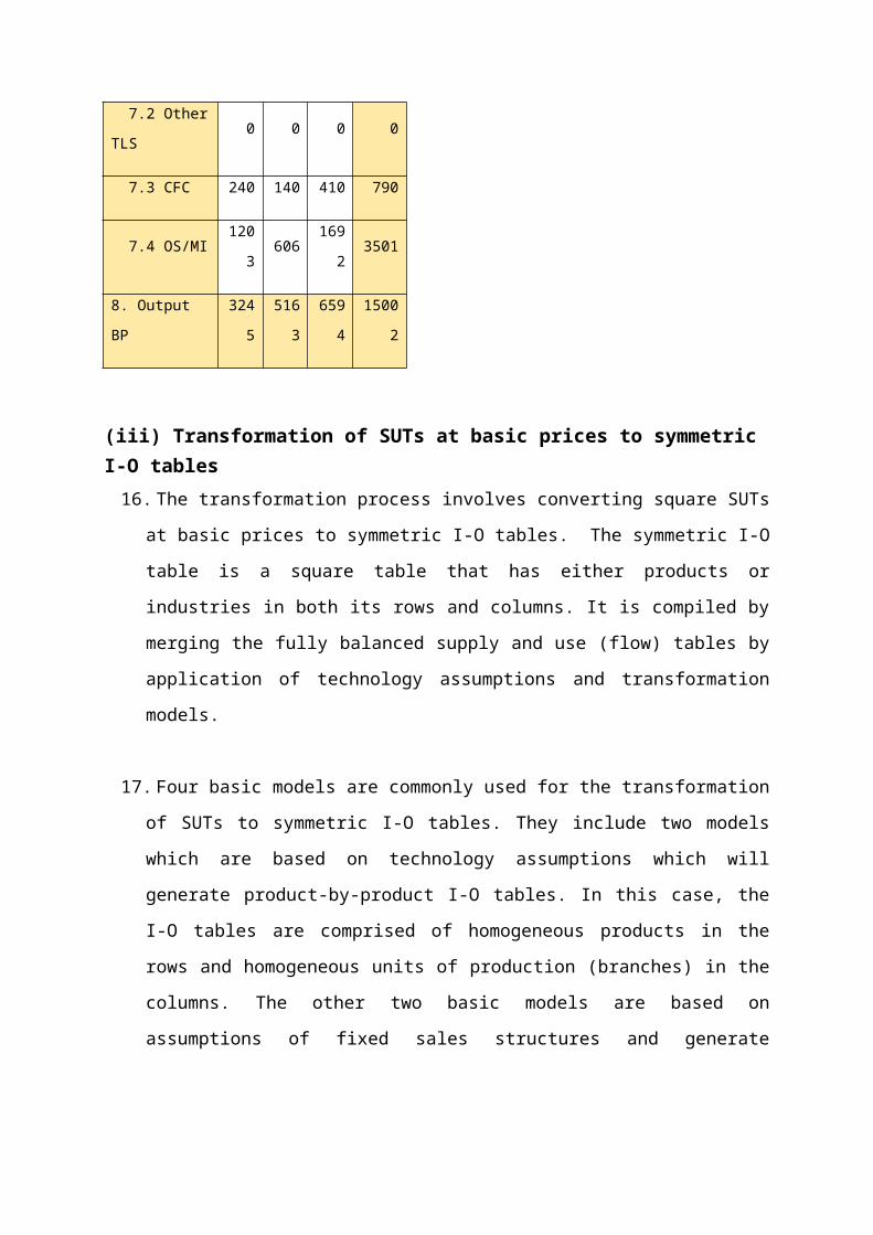
(iii) Transformation of SUTs at basic prices to symmetric I-O tables

16. The transformation process involves converting square SUTs at basic prices to

symmetric I-O tables. The symmetric I-O table is a square table that has either products

or industries in both its rows and columns. It is compiled by merging the fully balanced

supply and use (flow) tables by application of technology assumptions and

transformation models.

17. Four basic models are commonly used for the transformation of SUTs to symmetric I-O

tables. They include two models which are based on technology assumptions which will

generate product-by-product I-O tables. In this case, the I-O tables are comprised of

homogeneous products in the rows and homogeneous units of production (branches) in

the columns. The other two basic models are based on assumptions of fixed sales

structures and generate industry-by-industry I-O tables. The results are I-O tables with

products provided by industries in the rows and industries in the columns.

18. The reason that manipulation of SUTs is needed to produce an I-O table is the existence

of secondary products. There are three types of secondary production:

(a) Subsidiary products: those that are technologically unrelated to the primary product;

(b) By-products: products that are produced simultaneously with another product but

which can be regarded as secondary to that product;

(c) Joint products: products that are produced simultaneously with another product that

cannot be said to be secondary (for example beef and hides).

19. If there were the same number of industries as products, and if each industry only

produced one product5, the supply table for the domestic economy would be

unnecessary; the column totals for industries would be numerically equal to the row

totals for products and the inter-industry matrix would be square as originally compiled.

Product by product tables

20. In a product × product table both rows and columns represent the product group

sectors. If the secondary products of an industry group along-with the inputs are

transferred to the industry group where they are the principal products, the resulting

table is a product by product I-O table. There are two ways in which a product by

product matrix can be derived. These are:

(a) The industry technology assumption where each industry has its own specific means

of production irrespective of its product mix.

(b) The product technology assumption where each product is produced in its own

specific way irrespective of the industry where it is produced.

5Establishments are expected to produce single products while enterprises have secondary products.Ideally, statistical offices are expected to collect data from kind of activity units (KAUs), which typically produce single products, but in practice it is difficult to identify such units or for establishments to provide data for such units located within the establishments.

21. Under the industry technology assumption, the coefficients showing how manufactured

products are produced are assumed to depend on the industry they happen to be

produced in. It is assumed that the input structure of all products (both principal and

secondary) put out by a particular activity is the same, so the input structure associated

with a particular product may differ depending on which activity produces it. The

industry-technology assumption is always applied in conjunction with the "market share

hypothesis". It states that industries have fixed shares in the supply of products. This

combination of assumptions implies that the use of product i in the production of

product j is a weighted average of the use of product i by the various industries, the

weights being the shares of the industries in total supply of product j.

22. Under the product technology assumption, the coefficients showing how manufactured

products are produced are those of the manufacturing industry regardless of where they

are actually produced. It is assumed that there are specific input structures for particular

products, i.e. the input structure of a particular product is assumed to be the same

regardless of where (in which activity) it is produced.Usually product technology

assumption is followed for subsidiary products and industry technology assumption is

appropriate for joint products and by-products.

Industry by industry tables

23. In an industry × industry table, on the other hand, both rows and columns represent

industry group sectors comprising of a mix of different product groups. The row of a

sector in this table gives the supply of all products and secondary product (as a mix)

produced by the corresponding industry group for different intermediate and final uses.

Just as in the case of above matrix, there are two ways in which an industry by industry

matrix can be derived. These are:

(a) The fixed product sales structure where it is assumed the allocation of demand to

users depends on the product and not the industry from where it is sold.

(b) The fixed industry sales structure where it is assumed that users always demand the

same mix of products from an industry.

24. Thus, the four basic transformation models are based on the following assumptions:

1) Product technology assumption (Model A)

o Each product is produced in its own specific way, irrespective of the industry

where it is produced.

2) Industry technology assumption (Model B)

o Each industry has its own specific way of production, irrespective of its

product mix.

3) Fixed industry sales structure assumption (Model C)

o Each industry has its own specific sales structure, irrespective of its product

mix.

4) Fixed product sales structure assumption (Model D)

o Each product has its own specific sales structure, irrespective of the industry

where it is produced.

Options (1) and (3) may result in negative entries;

Options (2) and (4) do not contain any negative entries.

25. Both product by product and industry by industry tables could be compiled through the

matrix manipulations. While industry by industry I-O tables are close to statistical

sources and more heterogeneous in terms of input structures, product by product I-O

tables are believed to be more homogeneous in terms of cost structures. The choice of

empirical research for modelling and impact analysis, determines which type of I-O

tables should be compiled and used. All the four types of I-O tables serve different

analytical functions. For example, to ensure that price indices are strictly consistent, a

product by product table is preferred. For a link to labour market questions, an industry

by industry table may be more useful.

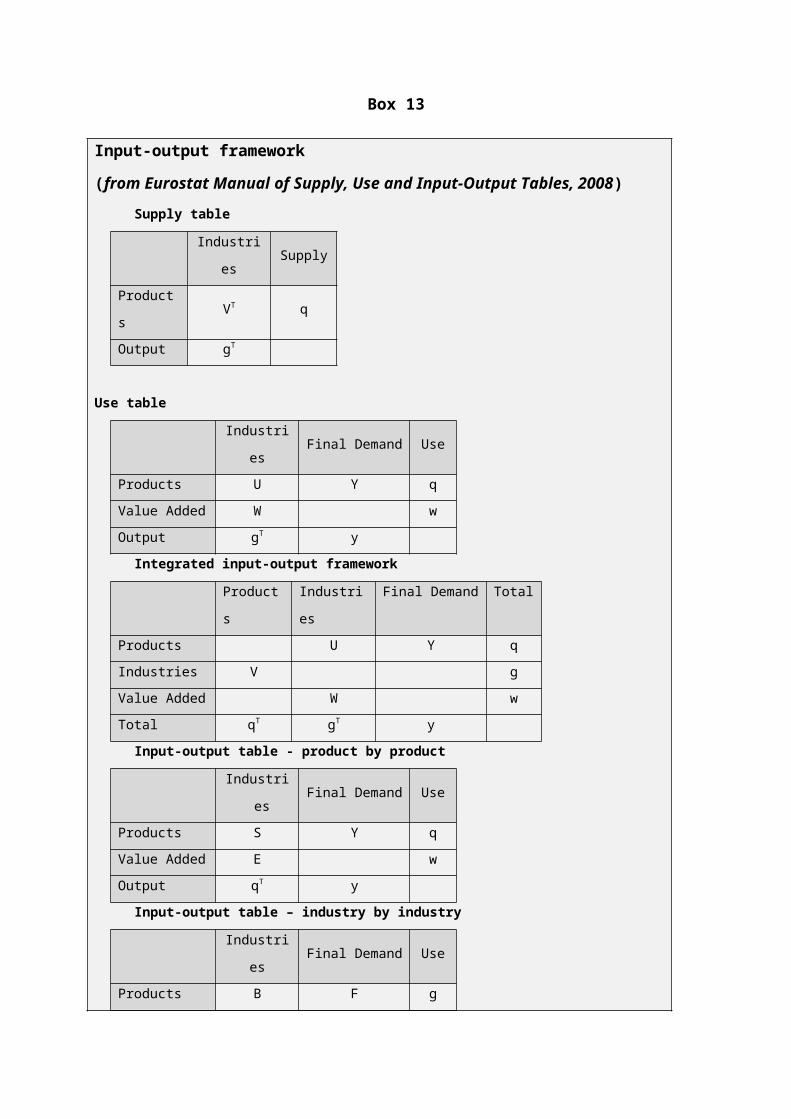
26. The following three boxes present the input-output framework, summary of

transformation models and an example with a simple 3-sector SUT for the SUT

described in Tables 16 and 22. The first two boxes are from the Eurostat Manual of

Supply, Use and Input-Output Tables, 2008.

Box 13

Input-output framework

(from Eurostat Manual of Supply, Use and Input-Output Tables, 2008) Supply table

Industries Supply

Products VT q

Output gT

Use table

Industries Final Demand Use

Products U Y q

Value Added W w

Output gT y

Integrated input-output framework

Products Industries Final Demand Total

Products U Y q

Industries V g

Value Added W w

Total qT gT y

Input-output table - product by product


Products S Y q

Value Added E w

Output qT y

Input-output table – industry by industry


Products B F g

Value Added W w

Output gT y

LEGEND

V = Make matrix - transpose of supply matrix (industry by product) y = Vector of final demand

VT = Supply matrix (product by industry) w = Vector of value added

U = Use matrix for intermediates (product by industry) I = Unit matrix

Y = Final demand matrix (product by category) q = Column vector of product

output

F = Final demand matrix (industry by category) qT = Row vector of product output

S = Matrix for intermediates (product by product) g = Column vector of industry

output

B = Matrix for intermediates (industry by industry) gT = Column vector of industry output

E = Value added matrix (components by homogenous branches)

W = Value added matrix (components by industry)

diag(q) = Diagonal matrix of product output

diag(g) = Diagonal matrix of industry output

INPUT COEFFICIENTS OF USE TABLE

Z = U * inv(diag(g)) Input requirements for products per unit of output of an industry (intermediates)

L = W * inv(diag(g)) Input requirements for value added per unit of output of an industry (primary input)

MARKET SHARE COEFFICIENTS OF SUPPLY TABLE

C = VT * inv(diag(g)) Product-mix matrix (share of each product in output of an industry)

D = V * inv(diag(q)) Market shares matrix (contribution of each industry to the output of a product)

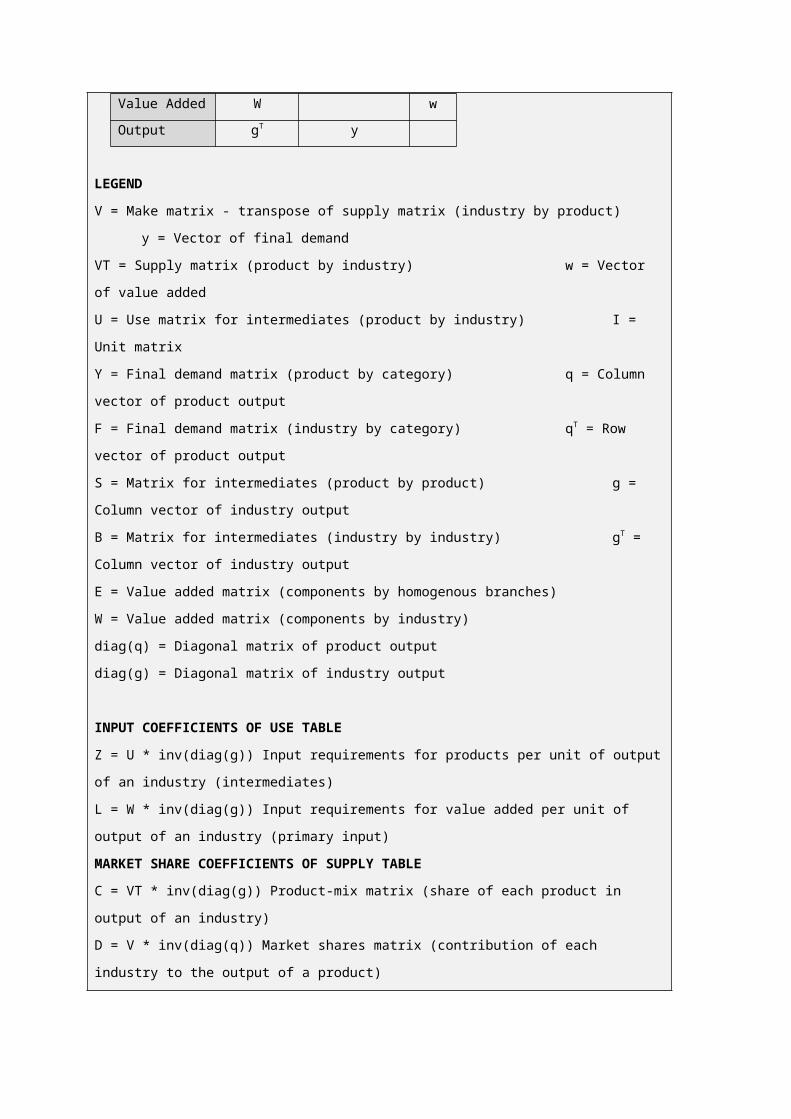
The main formulas of the four basic transformation models are summarised below.

Box 14

Summary of transformation models

MODEL A

Product

technology

Product-by-

product input-

output table

MODEL B

Industry technology

Product-by-product

input-output table

MODEL C

Fixed industry sales

structure

Industry-by-industry

input-output table

MODEL D

Fixed product sales

structure

Industry-by-industry

input-output table

Transformation

matrix

T = inv(V’) *

diag(q)

T = inv[diag(g)] *

V T = diag(g) * inv(V’) T = V * inv[diag(q)]

Input coefficients

A = U * T *

inv[diag(q)]

A = U * T *

inv[diag (q)]

A = T * U * inv[diag

(g)]

A = T * U * inv[diag

(g)]

Intermediates S = U * T S = U * T B = T * U B = T * U

Value added E = W * T E = W * T W = W W = W

Final demand Y = Y Y = Y F = T * Y F = T * Y

Output q = inv(I - A) * y q = inv(I - A) * y g = inv(I - A) * y g = inv(I - A) * y

27. From this tabulation it becomes clear that the four basic models have the following

features:

Product-by-product I-O tables are compiled by post-multiplying the use matrix and

value added matrix with a transformation matrix reflecting either product technology

or industry technology. Here, the final demand quadrant does not undergo any

transformation as their values are already in terms of products.

Industry-by-industry I-O tables can be derived from the supply and use system by pre-

multiplying the use matrix and final use matrix with a transformation matrix reflecting

either the fixed industry sales structure or fixed product sales structure. Here, the

value added quadrant does not undergo any transformation as their values are already

in terms of industries.

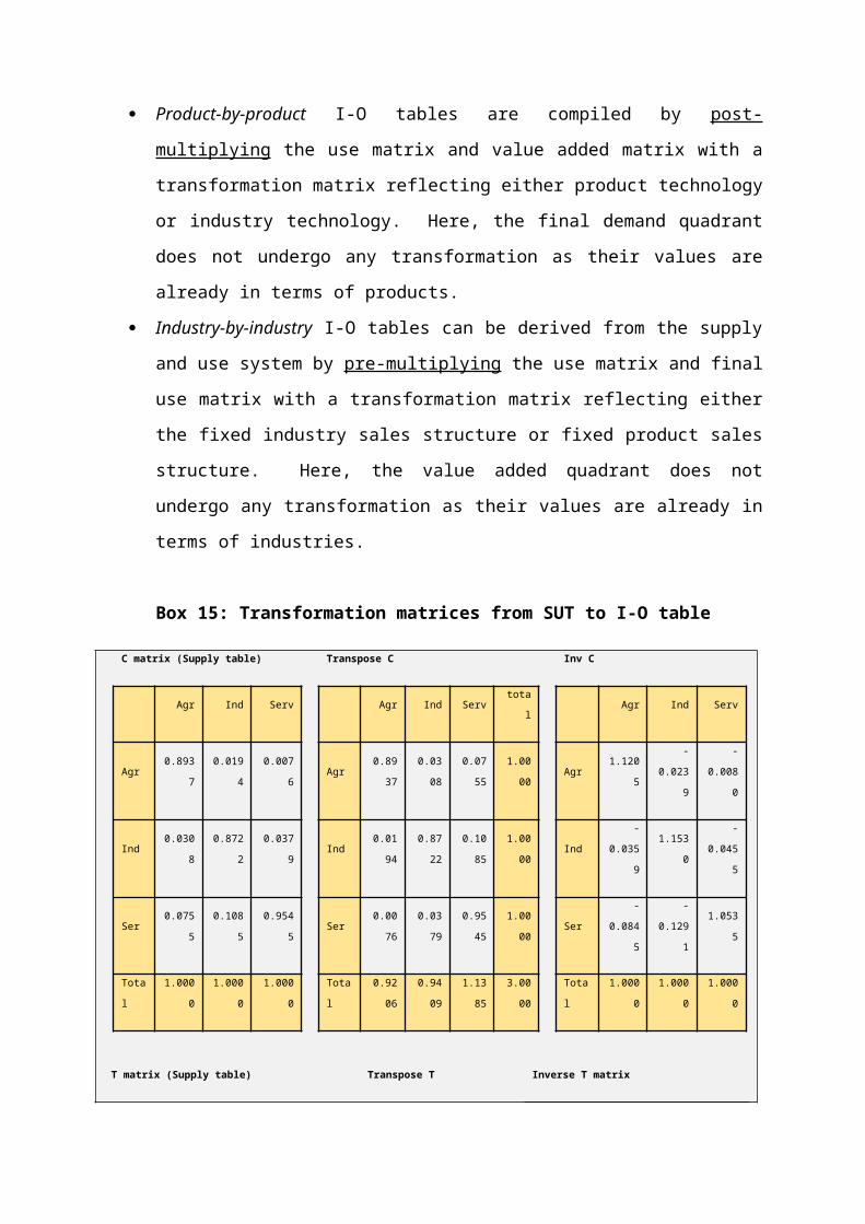
Box 15: Transformation matrices from SUT to I-O table

C matrix (Supply table) Transpose C Inv C

Agr Ind Serv Agr Ind Serv total Agr Ind Serv

Agr 0.8937 0.0194 0.0076 Agr 0.8937 0.0308 0.0755 1.0000 Agr 1.1205 -0.0239 -0.0080

Ind 0.0308 0.8722 0.0379 Ind 0.0194 0.8722 0.1085 1.0000 Ind -0.0359 1.1530 -0.0455

Ser 0.0755 0.1085 0.9545 Ser 0.0076 0.0379 0.9545 1.0000 Ser -0.0845 -0.1291 1.0535

Total 1.0000 1.0000 1.0000 Total 0.9206 0.9409 1.1385 3.0000 Total 1.0000 1.0000 1.0000

T matrix (Supply table) Transpose T Inverse T matrix

Agr Ind Serv total Agr Ind Serv Agr Ind Serv total

Agr 0.9508 0.0328 0.0164 1.0000 Agr 0.9508 0.0206 0.0345 Agr 1.0531 -0.0357 -0.0174 1.0000

Ind 0.0206 0.9279 0.0515 1.0000 Ind 0.0328 0.9279 0.0789 Ind -0.0212 1.0838 -0.0626 1.0000

Ser 0.0345 0.0789 0.8866 1.0000 Ser 0.0164 0.0515 0.8866 Ser -0.0391 -0.0950 1.1341 1.0000

Total 1.0059 1.0396 0.9545 3.0000 Total 1.0000 1.0000 1.0000 Total 0.9928 0.9530 1.0542 3.0000

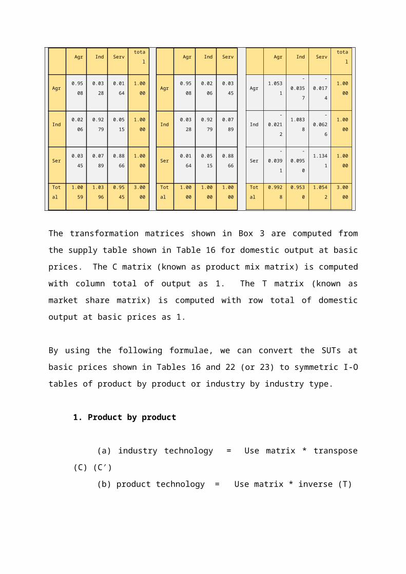
The transformation matrices shown in Box 3 are computed from the supply table shown in

Table 16 for domestic output at basic prices. The C matrix (known as product mix matrix) is

computed with column total of output as 1. The T matrix (known as market share matrix) is

computed with row total of domestic output at basic prices as 1.

By using the following formulae, we can convert the SUTs at basic prices shown in Tables 16

and 22 (or 23) to symmetric I-O tables of product by product or industry by industry type.

1. Product by product

(a) industry technology = Use matrix * transpose (C) (C′)

(b) product technology = Use matrix * inverse (T)

In both cases, there will be no change in the final demand vectors from the use table

of product by industry at basic prices, as these are already in terms of products.

2. Industry by industry

(a) fixed product sales structure = Transpose (T) (T′) * Use matrix

(b) fixed industry sales structure = Inverse (C) * Use matrix

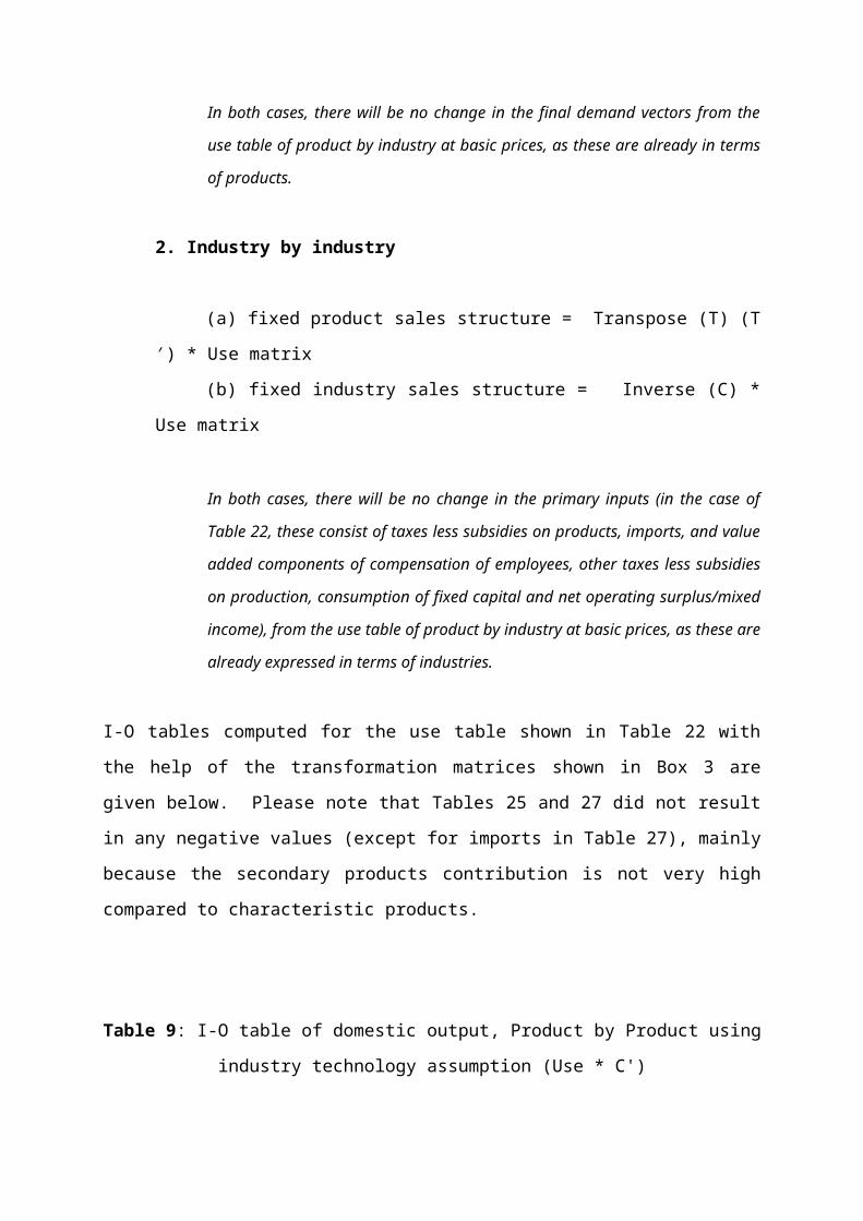
In both cases, there will be no change in the primary inputs (in the case of Table 22,

these consist of taxes less subsidies on products, imports, and value added

components of compensation of employees, other taxes less subsidies on production,

consumption of fixed capital and net operating surplus/mixed income), from the use

table of product by industry at basic prices, as these are already expressed in terms of

industries.

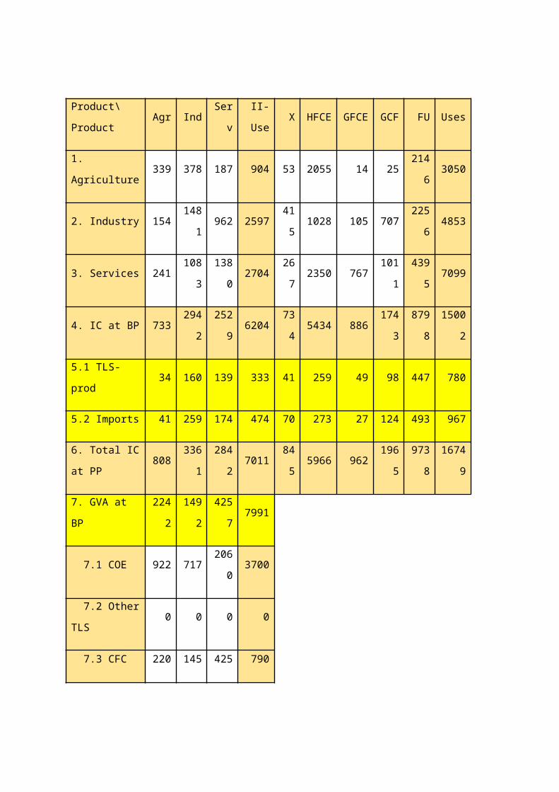
I-O tables computed for the use table shown in Table 22 with the help of the transformation

matrices shown in Box 3 are given below. Please note that Tables 25 and 27 did not result in

any negative values (except for imports in Table 27), mainly because the secondary products

contribution is not very high compared to characteristic products.

Table 9: I-O table of domestic output, Product by Product using industry technology

assumption (Use * C')

Product\Product Agr Ind ServII-

UseX HFCE GFCE GCF FU Uses

1. Agriculture 339 378 187 904 53 2055 14 25214

63050

2. Industry 154 1481 962 259741

51028 105 707

225

64853

3. Services 241 1083 1380 270426

72350 767 1011

439

57099

4. IC at BP 733 2942 2529 620473

45434 886 1743

879

815002

5.1 TLS-prod 34 160 139 333 41 259 49 98 447 780

5.2 Imports 41 259 174 474 70 273 27 124 493 967

6. Total IC at

PP808 3361 2842 7011

84

55966 962 1965

973

816749

7. GVA at BP 2242 1492 4257 7991

7.1 COE 922 717 2060 3700

7.2 Other TLS 0 0 0 0

7.3 CFC 220 145 425 790

7.4 OS/MI 1100 630 1772 3501

8. Output - BP 3050 4853 7099 15002

Table 10: I-O table of domestic output, Product by Product using product technology

assumption (Use * T-1)



1. Agriculture 375 425 104 904 53 2055 14 25 3050

2. Industry 70 1716 812 2597 415 1028 105 707 4853

3. Services 170 1145 1389 2704 267 2350 767 1011 7099

4. IC at BP 614 3286 2304 6204 734 5434 886 1743 15002

5.1 TLS-prod 26 179 128 333 41 259 49 98 780

5.2 Imports 28 298 148 474 70 273 27 124 967

6. Total IC at PP 668 3763 2580 7011 845 5966 962 1965 16749

7. GVA at BP (8-6)238

21090 4519 7991

7.1 COE 960 533 2207 3700

7.2 Other TLS 0 0 0 0

7.3 CFC 234 104 452 790

7.4 OS/MI118

8453 1860 3501

8. output BP305

04853 7099 15002

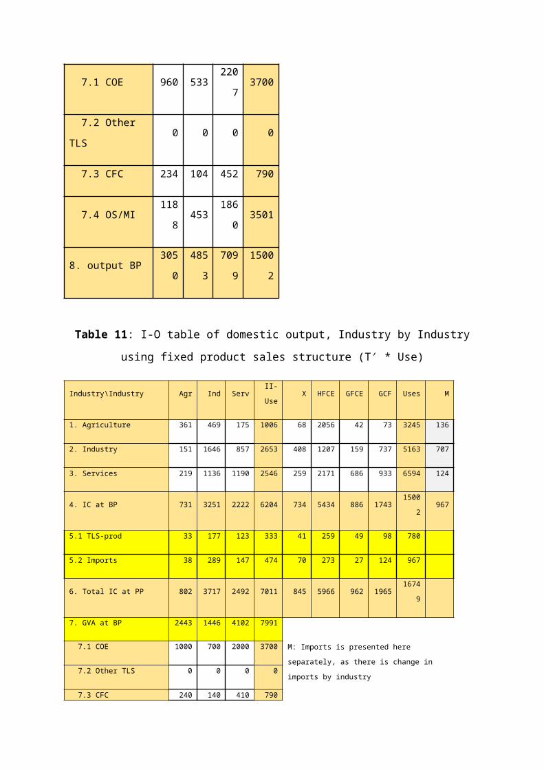
Table 11: I-O table of domestic output, Industry by Industry using fixed product sales

structure (T′ * Use)

Industry\Industry Agr Ind ServII-

UseX HFCE

GFC

EGCF Uses M

1. Agriculture 361 469 175 1006 68 2056 42 73 3245 136

2. Industry 151 1646 857 2653 408 1207 159 737 5163 707

3. Services 219 1136 1190 2546 259 2171 686 933 6594 124

4. IC at BP 731 3251 2222 6204 734 5434 886 1743 15002 967

5.1 TLS-prod 33 177 123 333 41 259 49 98 780

5.2 Imports 38 289 147 474 70 273 27 124 967

6. Total IC at PP 802 3717 2492 7011 845 5966 962 1965 16749

7. GVA at BP 2443 1446 4102 7991

M: Imports is presented here separately, as there is

change in imports by industry 7.1 COE 1000 700 2000 3700

7.2 Other TLS 0 0 0 0

7.3 CFC 240 140 410 790

7.4 OS/MI 1203 606 1692 3501

8. Output BP 3245 5163 6594 15002

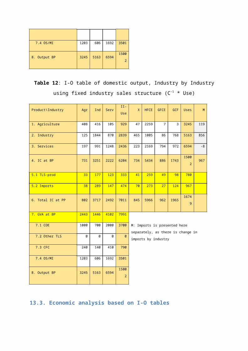
Table 12: I-O table of domestic output, Industry by Industry using fixed industry sales

structure (C-1 * Use)


UseX HFCE

GFC

EGCF Uses M

1. Agriculture 408 416 105 929 47 2259 7 3 3245 119

2. Industry 125 1844 870 2839 465 1005 86 768 5163 856

3. Services 197 991 1248 2436 223 2169 794 972 6594 -8

4. IC at BP 731 3251 2222 6204 734 5434 886 1743 15002 967

5.1 TLS-prod 33 177 123 333 41 259 49 98 780

5.2 Imports 38 289 147 474 70 273 27 124 967

6. Total IC at PP 802 3717 2492 7011 845 5966 962 1965 16749

7. GVA at BP 2443 1446 4102 7991

7.1 COE 1000 700 2000 3700

M: Imports is presented here separately, as there is

change in imports by industry

7.2 Other TLS 0 0 0 0

7.3 CFC 240 140 410 790

7.4 OS/MI 1203 606 1692 3501

8. Output BP 3245 5163 6594 15002

13.3. Economic analysis based on I-O tables

28. For economic analysis, illustration given in this chapter is based on Table 24, which is

product by product with industry technology assumption. Analysis can be done with

any other three I-O tables6 following same sequence of steps given in this Section. The

text for the conceptual part of this Section has mainly been drawn from the Eurostat

Manual of Supply, Use and Input-Output Tables (Eurostat, 2008)7.

29. The researchers, businesses and government policy makers would like to understand the

inter-industry linkages, linkages between final uses and output and impact of policy

decisions in the economy in terms of employment, income and taxes it generates and

also what capital and imports it needs to grow. The impact analysis can be in terms of

how other industries depend on the industry under study or how this industry impacts on

other industries. An I-O model enables these impact analyses as this model in its

simplest form is a full articulation of inter-industry analysis and facilitates impact

analysis8.

(a) I-O Models

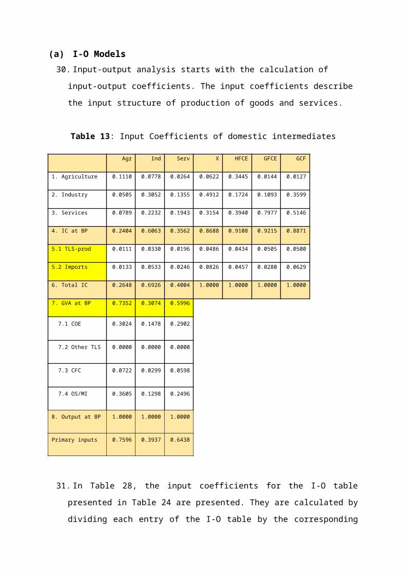
30. Input-output analysis starts with the calculation of input-output coefficients. The input

coefficients describe the input structure of production of goods and services.

Table 13: Input Coefficients of domestic intermediates6After correcting for negative entries, if any.7 The objective of the Eurostat Manual is to provide guidance for national accountants who are engaged to establish an input-output framework for their economy according to international standards.8The Input-output analysis was founded by Wassily Leontief in the thirties of this century.

Agr Ind Serv X HFCE GFCE GCF

1. Agriculture 0.1110 0.0778 0.0264 0.0622 0.3445 0.0144 0.0127

2. Industry 0.0505 0.3052 0.1355 0.4912 0.1724 0.1093 0.3599

3. Services 0.0789 0.2232 0.1943 0.3154 0.3940 0.7977 0.5146

4. IC at BP 0.2404 0.6063 0.3562 0.8688 0.9108 0.9215 0.8871

5.1 TLS-prod 0.0111 0.0330 0.0196 0.0486 0.0434 0.0505 0.0500

5.2 Imports 0.0133 0.0533 0.0246 0.0826 0.0457 0.0280 0.0629

6. Total IC 0.2648 0.6926 0.4004 1.0000 1.0000 1.0000 1.0000

7. GVA at BP 0.7352 0.3074 0.5996

7.1 COE 0.3024 0.1478 0.2902

7.2 Other TLS 0.0000 0.0000 0.0000

7.3 CFC 0.0722 0.0299 0.0598

7.4 OS/MI 0.3605 0.1298 0.2496

8. Output at BP 1.0000 1.0000 1.0000

Primary inputs 0.7596 0.3937 0.6438

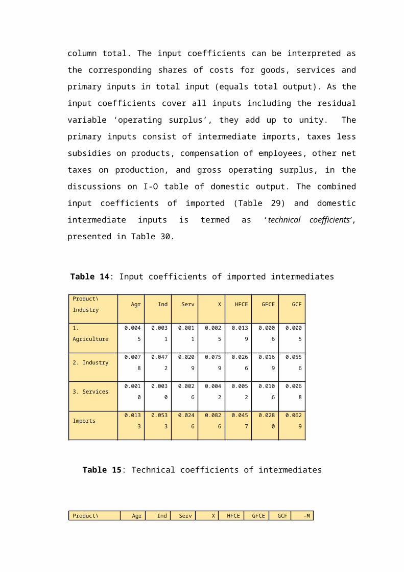
31. In Table 28, the input coefficients for the I-O table presented in Table 24 are presented.

They are calculated by dividing each entry of the I-O table by the corresponding column

total. The input coefficients can be interpreted as the corresponding shares of costs for

goods, services and primary inputs in total input (equals total output). As the input

coefficients cover all inputs including the residual variable ‘operating surplus’, they add

up to unity. The primary inputs consist of intermediate imports, taxes less subsidies on

products, compensation of employees, other net taxes on production, and gross

operating surplus, in the discussions on I-O table of domestic output. The combined

input coefficients of imported (Table 29) and domestic intermediate inputs is termed as

‘technical coefficients’, presented in Table 30.

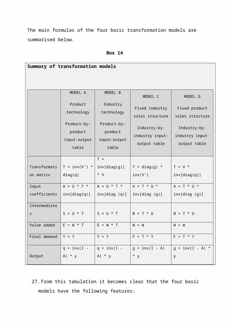
Table 14: Input coefficients of imported intermediates

Product\Industry Agr Ind Serv X HFCE GFCE GCF

1. Agriculture 0.0045 0.0031 0.0011 0.0025 0.0139 0.0006 0.0005

2. Industry 0.0078 0.0472 0.0209 0.0759 0.0266 0.0169 0.0556

3. Services 0.0010 0.0030 0.0026 0.0042 0.0052 0.0106 0.0068

Imports 0.0133 0.0533 0.0246 0.0826 0.0457 0.0280 0.0629

Table 15: Technical coefficients of intermediates

Product\Industry Agr Ind Serv X HFCE GFCE GCF -M

1. Agriculture 0.1155 0.0810 0.0274 0.0647 0.3584 0.0150 0.0132 0.1272

2. Industry 0.0583 0.3524 0.1564 0.5671 0.1990 0.1262 0.4155 0.7756

3. Services 0.0800 0.2262 0.1969 0.3196 0.3992 0.8083 0.5214 0.0972

4. IC at BP 0.2537 0.6595 0.3808 0.9514 0.9566 0.9495 0.9500 1.0000

5.1 TLS-prod 0.0111 0.0330 0.0196 0.0486 0.0434 0.0505 0.0500

6. Total IC at PP 0.2648 0.6926 0.4004 1.0000 1.0000 1.0000 1.0000 1.0000

7. GVA at BP 0.7352 0.3074 0.5996

7.1 COE 0.3024 0.1478 0.2902

7.2 Other TLS 0.0000 0.0000 0.0000

7.3 CFC 0.0722 0.0299 0.0598

7.4 OS/MI 0.3605 0.1298 0.2496

8. Output BP 1.0000 1.0000 1.0000

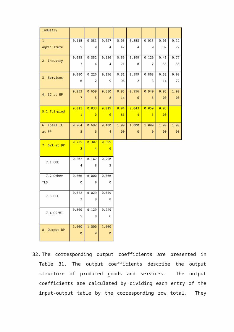
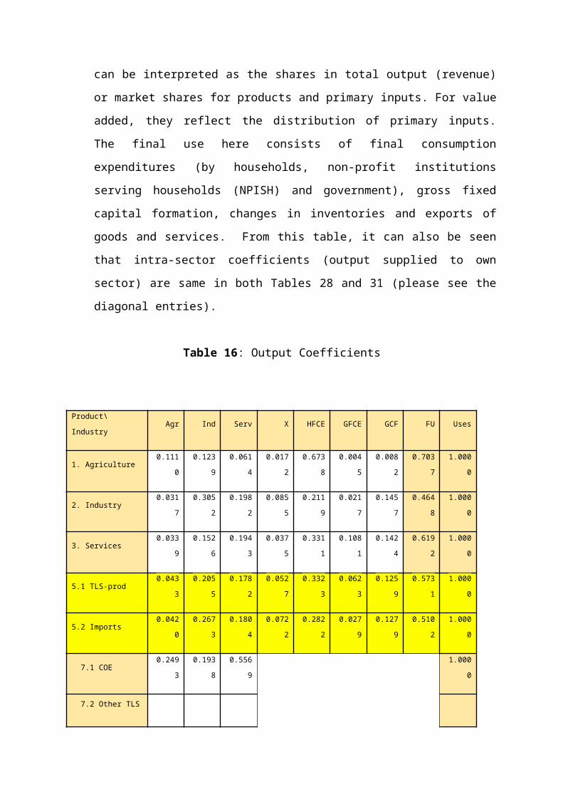
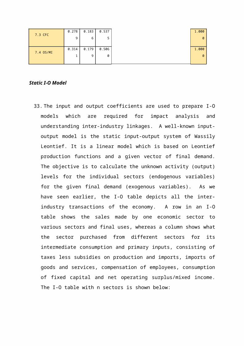
32. The corresponding output coefficients are presented in Table 31. The output coefficients

describe the output structure of produced goods and services. The output coefficients

are calculated by dividing each entry of the input-output table by the corresponding row

total. They can be interpreted as the shares in total output (revenue) or market shares

for products and primary inputs. For value added, they reflect the distribution of

primary inputs. The final use here consists of final consumption expenditures (by

households, non-profit institutions serving households (NPISH) and government), gross

fixed capital formation, changes in inventories and exports of goods and services. From

this table, it can also be seen that intra-sector coefficients (output supplied to own

sector) are same in both Tables 28 and 31 (please see the diagonal entries).

Table 16: Output Coefficients

Product\Industry Agr Ind Serv X HFCE GFCE GCF FU Uses

1. Agriculture 0.1110 0.1239 0.0614 0.0172 0.6738 0.0045 0.0082 0.7037 1.0000

2. Industry 0.0317 0.3052 0.1982 0.0855 0.2119 0.0217 0.1457 0.4648 1.0000

3. Services 0.0339 0.1526 0.1943 0.0375 0.3311 0.1081 0.1424 0.6192 1.0000

5.1 TLS-prod 0.0433 0.2055 0.1782 0.0527 0.3323 0.0623 0.1259 0.5731 1.0000

5.2 Imports 0.0420 0.2673 0.1804 0.0722 0.2822 0.0279 0.1279 0.5102 1.0000

7.1 COE 0.2493 0.1938 0.5569 1.0000

7.2 Other TLS

7.3 CFC 0.2789 0.1836 0.5375 1.0000

7.4 OS/MI 0.3141 0.1799 0.5060 1.0000

Static I-O Model

33. The input and output coefficients are used to prepare I-O models which are required for

impact analysis and understanding inter-industry linkages. A well-known input-output

model is the static input-output system of Wassily Leontief. It is a linear model which is

based on Leontief production functions and a given vector of final demand. The

objective is to calculate the unknown activity (output) levels for the individual sectors

(endogenous variables) for the given final demand (exogenous variables). As we have

seen earlier, the I-O table depicts all the inter-industry transactions of the economy. A

row in an I-O table shows the sales made by one economic sector to various sectors and

final uses, whereas a column shows what the sector purchased from different sectors for

its intermediate consumption and primary inputs, consisting of taxes less subsidies on

production and imports, imports of goods and services, compensation of employees,

consumption of fixed capital and net operating surplus/mixed income. The I-O table

with n sectors is shown below:

Intermediate uses Final uses Gross

output123......j.....n Consumptionexpenditure capital

formation

Exports

1 x 11 x 12 ....xiJ....x1n c1 f1 e1 X1

2 x 21 x 22 ....x2j....x 2n c2 f2 e2 X2

. ............................... . . . .

. .............................. . . . .

i x i1 x i2.......x ij......x

in

ci f i ei Xi

. . ............................. . . . .

n x n1 x n2......xnj.....x

nn

cn fn en Xn

Primary

inputs

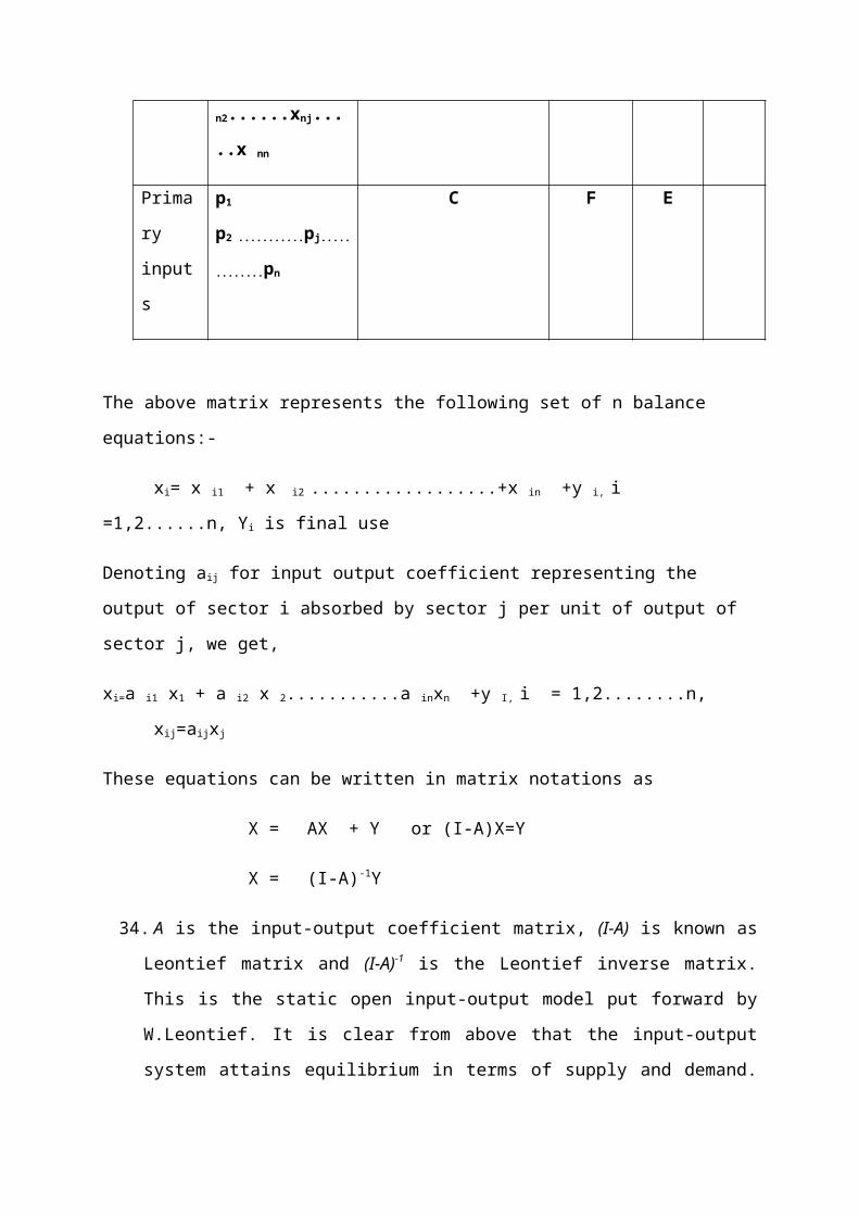
p1 p2 ...........pj.............pn C F E

The above matrix represents the following set of n balance equations:-

xi= x i1 + x i2 ..................+x in +y i, i =1,2......n, Yi is final use

Denoting aij for input output coefficient representing the output of sector i absorbed by sector j

per unit of output of sector j, we get,

xi=a i1 x1 + a i2 x 2...........a inxn +y I, i = 1,2........n, xij=aijxj

These equations can be written in matrix notations as

X = AX + Y or (I-A)X=Y

X = (I-A)-1Y

34. A is the input-output coefficient matrix, (I-A) is known as Leontief matrix and (I-A)-1 is

the Leontief inverse matrix. This is the static open input-output model put forward by

W.Leontief. It is clear from above that the input-output system attains equilibrium in

terms of supply and demand. Thus, the input-output analysis is an economic application

of general equilibrium theory, having the coefficient matrix A, known from earlier I-O

tables and for a given final demand vector y, the model determines the output level x for

the economy.

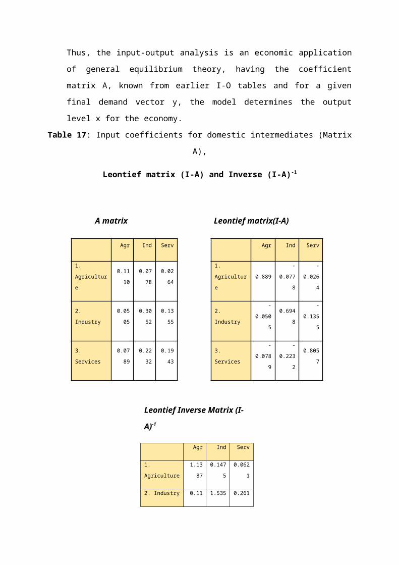
Table 17: Input coefficients for domestic intermediates (Matrix A),

Leontief matrix (I-A) and Inverse (I-A)-1

A matrix Leontief matrix(I-A)

Agr Ind Serv Agr Ind Serv

1. Agriculture 0.1110 0.0778 0.0264 1. Agriculture 0.889 -0.0778 -0.0264

2. Industry 0.0505 0.3052 0.1355 2. Industry -0.0505 0.6948 -0.1355

3. Services 0.0789 0.2232 0.1943 3. Services -0.0789 -0.2232 0.8057

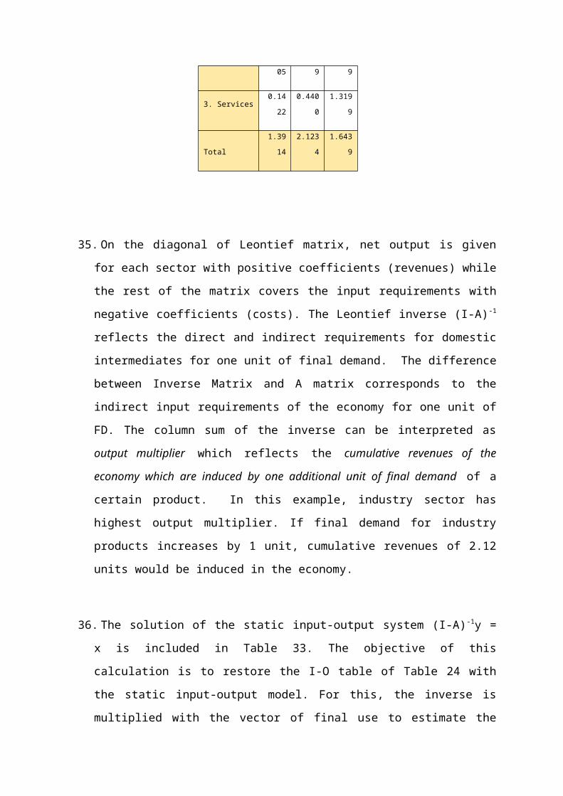
Leontief Inverse Matrix (I-A)-1

Agr Ind Serv

1. Agriculture 1.1387 0.1475 0.0621

2. Industry 0.1105 1.5359 0.2619

3. Services 0.1422 0.4400 1.3199

Total 1.3914 2.1234 1.6439

35. On the diagonal of Leontief matrix, net output is given for each sector with positive

coefficients (revenues) while the rest of the matrix covers the input requirements with

negative coefficients (costs). The Leontief inverse (I-A)-1 reflects the direct and indirect

requirements for domestic intermediates for one unit of final demand. The difference

between Inverse Matrix and A matrix corresponds to the indirect input requirements of

the economy for one unit of FD. The column sum of the inverse can be interpreted as

output multiplier which reflects the cumulative revenues of the economy which are

induced by one additional unit of final demand of a certain product. In this example,

industry sector has highest output multiplier. If final demand for industry products

increases by 1 unit, cumulative revenues of 2.12 units would be induced in the

economy.

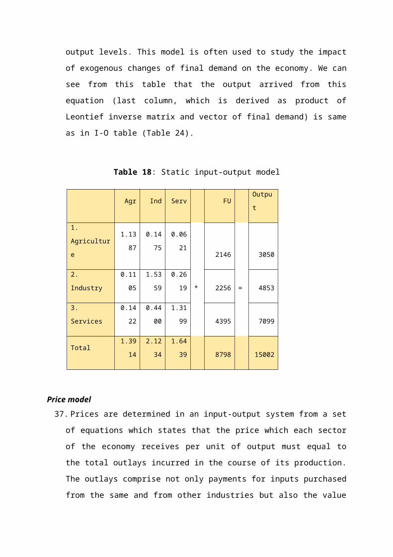
36. The solution of the static input-output system (I-A)-1y = x is included in Table 33. The

objective of this calculation is to restore the I-O table of Table 24 with the static input-

output model. For this, the inverse is multiplied with the vector of final use to estimate

the output levels. This model is often used to study the impact of exogenous changes of

final demand on the economy. We can see from this table that the output arrived from

this equation (last column, which is derived as product of Leontief inverse matrix and

vector of final demand) is same as in I-O table (Table 24).

Table 18: Static input-output model

Agr Ind Serv FU Output

1. Agriculture 1.138 0.1475 0.0621 2146 3050

7

2. Industry0.110

51.5359 0.2619

* 2256 = 4853

3. Services0.142

20.4400 1.3199

4395 7099

Total1.391

42.1234 1.6439

8798 15002

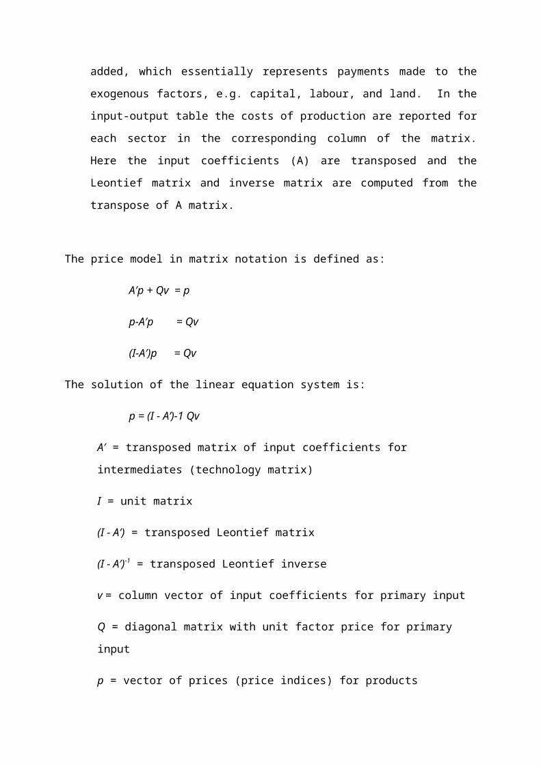
Price model37. Prices are determined in an input-output system from a set of equations which states that

the price which each sector of the economy receives per unit of output must equal to the

total outlays incurred in the course of its production. The outlays comprise not only

payments for inputs purchased from the same and from other industries but also the

value added, which essentially represents payments made to the exogenous factors, e.g.

capital, labour, and land. In the input-output table the costs of production are reported

for each sector in the corresponding column of the matrix. Here the input coefficients

(A) are transposed and the Leontief matrix and inverse matrix are computed from the

transpose of A matrix.

The price model in matrix notation is defined as:

A′p + Qv = p

p-A′p = Qv

(I-A′)p = Qv

The solution of the linear equation system is:

p = (I - A’)-1 Qv

A′ = transposed matrix of input coefficients for intermediates (technology matrix)

I = unit matrix

(I - A′) = transposed Leontief matrix

(I - A′)-1 = transposed Leontief inverse

v = column vector of input coefficients for primary input

Q = diagonal matrix with unit factor price for primary input

p = vector of prices (price indices) for products

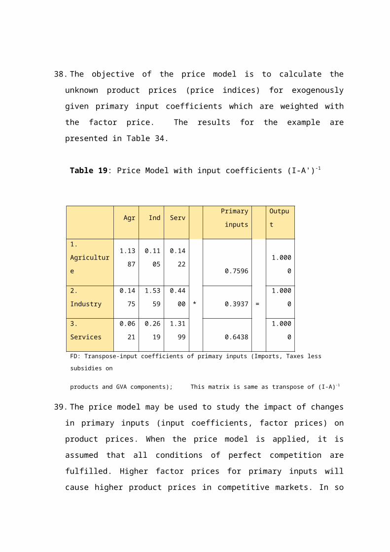
38. The objective of the price model is to calculate the unknown product prices (price

indices) for exogenously given primary input coefficients which are weighted with the

factor price. The results for the example are presented in Table 34.

Table 19: Price Model with input coefficients (I-A')-1

Agr Ind Serv Primary inputs Output

1. Agriculture1.138

70.1105

0.142

2 0.7596 1.0000

2. Industry0.147

51.5359

0.440

0 * 0.3937 = 1.0000

3. Services0.062

10.2619

1.319

9 0.6438 1.0000

FD: Transpose-input coefficients of primary inputs (Imports, Taxes less subsidies on

products and GVA components); This matrix is same as transpose of (I-A)-1

39. The price model may be used to study the impact of changes in primary inputs (input

coefficients, factor prices) on product prices. When the price model is applied, it is

assumed that all conditions of perfect competition are fulfilled. Higher factor prices for

primary inputs will cause higher product prices in competitive markets. In so far, the

approach is able to simulate the effects of a cost push type of inflation. For example, the

price model could be used to study the impact of an increase of the tax on gasoline on

other product prices.

Central model of input-output analysis40. In addition to studying the impact of final demand on output (quantity model) and value

added changes on prices (price model), I-O models can be extended to evaluate the

direct and indirect impact of economic policies on other economic variables such as

labour, capital, energy and emissions (joint product). The following extension of the

input-output equation system offers multiple approaches for analysis:

Z = B (I - A)-1Y Central equation system of input-output analysis

B = matrix of input coefficients for specific variable in economic analysis

(intermediates, labour, capital, energy, emissions, etc.)

I = unit matrix

A = matrix of input coefficients for intermediates

Y = diagonal matrix for final demand

Z = matrix with results for direct and indirect requirements (intermediates, labour,

capital, energy, emissions, etc.)

41. Matrix B includes the input coefficients of the variable under investigation

(intermediates, labour, capital, energy, emissions, etc.). The diagonal matrix Y denotes

exogenous final demand for goods and services. The matrix Z incorporates the results

for the direct and indirect requirements (intermediates, labour, capital, energy) or joint

products (emissions) for the produced goods and services. In essence, this approach

would allow assessing the total (direct and indirect) primary energy requirements or

carbon dioxide emissions for the production of a vehicle which can be observed at all

stages of production. Corresponding calculations of the labour and capital content of

products are also feasible. Direct contributions of final demand (for example direct

emissions of carbon dioxide by private households) must be added as column vector to

the results of matrix Z.

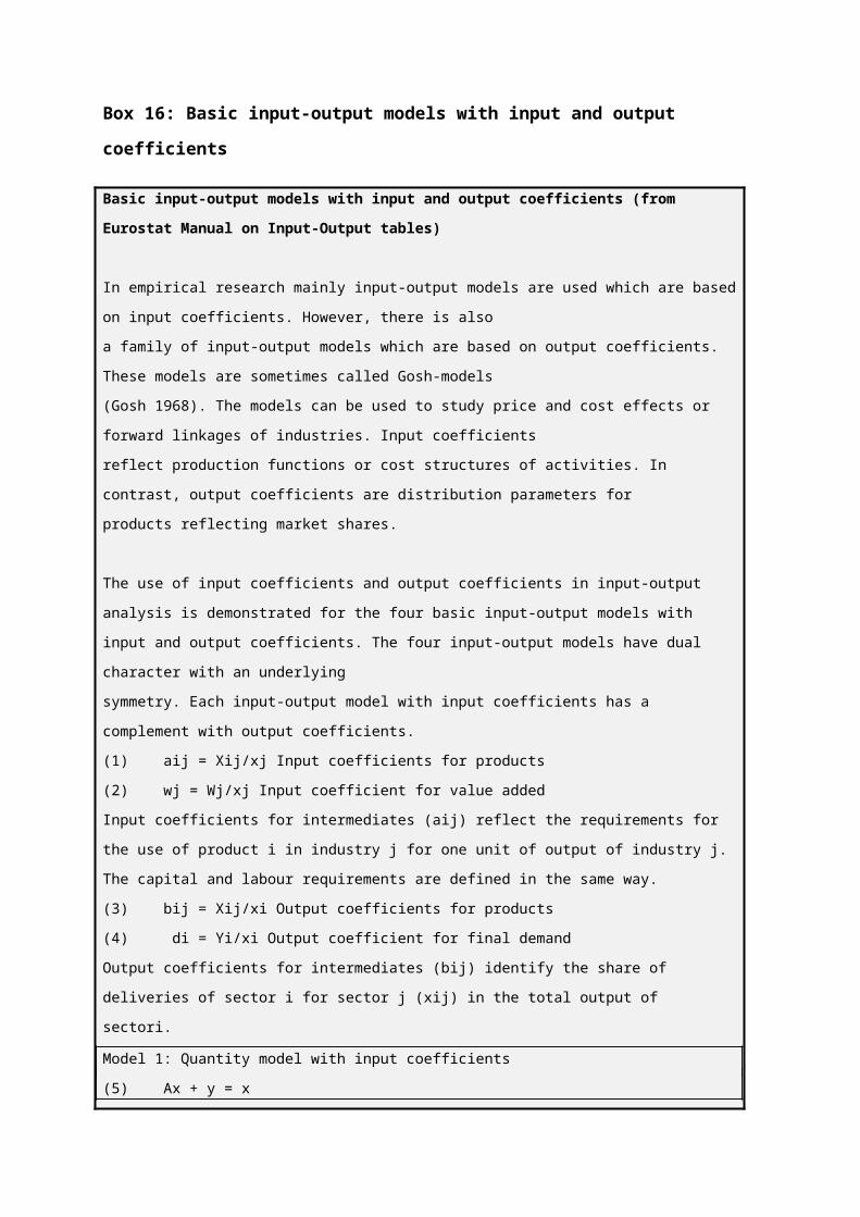
Box 16: Basic input-output models with input and output coefficients

Basic input-output models with input and output coefficients (from Eurostat Manual on Input-Output

tables)

In empirical research mainly input-output models are used which are based on input coefficients. However,

there is also

a family of input-output models which are based on output coefficients. These models are sometimes called

Gosh-models

(Gosh 1968). The models can be used to study price and cost effects or forward linkages of industries. Input

coefficients

reflect production functions or cost structures of activities. In contrast, output coefficients are distribution

parameters for

products reflecting market shares.

The use of input coefficients and output coefficients in input-output analysis is demonstrated for the four

basic input-output models with input and output coefficients. The four input-output models have dual

character with an underlying

symmetry. Each input-output model with input coefficients has a complement with output coefficients.

(1) aij = Xij/xj Input coefficients for products

(2) wj = Wj/xj Input coefficient for value added

Input coefficients for intermediates (aij) reflect the requirements for the use of product i in industry j for one

unit of output of industry j. The capital and labour requirements are defined in the same way.

(3) bij = Xij/xi Output coefficients for products

(4) di = Yi/xi Output coefficient for final demand

Output coefficients for intermediates (bij) identify the share of deliveries of sector i for sector j (xij) in the

total output of

sectori.

Model 1: Quantity model with input coefficients

(5) Ax + y = x

(6) (I - A)x = y

(7) x = (I - A)-1 y

A = Matrix of input coefficients for intermediates with A = aij for i,j = 1, 2, ..., m.

I = Unit matrix

x = Column vector of output for sectors 1 to m with x1, x2, …,xm.

y = Column vector of exogenous final demand by product with y1, y2, …,ym.

-----------------------------------------------------------------------------------------------------------------------------------

Model 2: Price model with input coefficients

(8) A’p + w = p

(9) (I - A’)p = w

(10) p = (I - A’)-1 w

A’ = Transposed matrix of input coefficients for intermediates with A = aij for i,j = 1, 2, ..., m.

I = Unit matrix

x = Column vector of unit product price indexes for sectors 1 to m with p1, p2, …, pm.

w = Column vector of exogenous input coefficients for value added w1, w2, …,wm.

-----------------------------------------------------------------------------------------------------------------------------------

Model 3: Price model with output coefficients

(11) Bp + d = p

(12) (I - B)p = d

(13) p = (I - B)-1 d

B = Matrix of output coefficients for intermediates with B = aij for i,j = 1, 2, ..., m.

I = Unit matrix

p = Column vector of unit product price indexes for sectors 1 to m with p1, p2, …, pm.

d = Column vector of exogenous output coefficients for final demand by product with d1, d2, …, dm

-----------------------------------------------------------------------------------------------------------------------------------

Model 4: Quantity model with output coefficients

(14) B’x + z = x

(15) (I - B’)x = z

(16) x = (I - B’)-1 z

B’ = Transposed matrix of output coefficients for intermediates with A = aij for i,j = 1, 2, ..., m.

I = Unit matrix

x = Column vector of product output for sectors 1 to m with x1, x2, …,xm.

z = Column vector of exogenous value added by sector with z1, z2, …,zm.

The dual character of the four input-output models is presented in Box below. It remains to be seen in

empirical research if input coefficients or output coefficients are more stable in time and behave according to

expectations. However, there are good reasons why input-output models with output coefficients are rarely

used in empirical research: they lack a proper microeconomic foundation. Input-output models with input

coefficients are well established in economic analysis. Such models reflect the cost structure of industries

and input structure of final demand components.

Box 17: Four basic models of input-output analysis

Four basic models of input-output analysis

Input-Output Table

Product\Product Agr Ind ServII-

UseX HFCE GFCE GCF FU Uses

1. Agriculture 339 378 187 904 53 2055 14 25 2146 3050

2. Industry 154 1481 962 2597 415 1028 105 707 2256 4853

3. Services 241 1083 1380 2704 267 2350 767101

14395 7099

GVA/Primary

input* 2317 1911 4570 8798 111 532 76 222 940 1747

Total input 3050 4853 7099 15002

* consists of imports and taxes less subsidies on products, besides GVA

Input Coefficients

Product\Product Agr Ind Serv

1. Agriculture 0.1110 0.0778 0.0264

2. Industry 0.0505 0.3052 0.1355

3. Services 0.0789 0.2232 0.1943

GVA/Primary

input*0.7596 0.3937 0.6438

Total input 1.0000 1.0000 1.0000

Output Coefficients

Agr Ind Serv FU Output

1.

Agriculture0.1110

0.123

90.0614

0.703

7 1.000

2. Industry 0.03170.305

20.1982

0.464

8 1.000

3. Services 0.03390.152

60.1943

0.619

2 1.000

A matrix (from input coefficients) Inverse Matrix ((I-A)-1)


1.

Agriculture 0.1110 0.0778 0.0264 1. Agriculture 1.1387 0.1475 0.0621

2. Industry 0.0505 0.3052 0.1355 2. Industry 0.1105 1.5359 0.2619

3. Services 0.0789 0.2232 0.1943 3. Services 0.1422 0.4400 1.3199

B matrix (from output coefficients) Inverse Matrix ((I-B)-1)


1. Agriculture 0.1110 0.1239 0.0614 1. Agriculture 1.1387 0.2348 0.1445

2. Industry 0.0317 0.3052 0.1982 2. Industry 0.0694 1.5359 0.3832

3. Services 0.0339 0.1526 0.1943 3. Services 0.0611 0.3008 1.3199

Box 18 (Contd.)

Model 1: Quantity model with input coefficients(I-A)-1

Agr Ind Serv

*

FU

=

Output

1. Agriculture 1.1387 0.1475 0.0621 2146 3050

2. Industry 0.1105 1.5359 0.2619 2256 4853

3. Services 0.1422 0.4400 1.3199 4395 7099

Total 1.3914 2.1234 1.6439 8798 15002

Model 2: Price model with input coefficients(I-A′)-1

Agr Ind Serv Primary inputs Output

1. Agriculture 1.1387 0.1105 0.1422 0.7596 1.0000

2. Industry 0.1475 1.5359 0.4400 * 0.3937 = 1.0000

3. Services 0.0621 0.2619 1.3199 0.6438 1.0000

Model 3: Price model with output coefficients(I-B)-1

Agr Ind Serv

*

FU

=

Output

1. Agriculture 1.1387 0.2348 0.1445 0.7037 1.0000

2. Industry 0.0694 1.5359 0.3832 0.4648 1.0000

3. Services 0.0611 0.3008 1.3199 0.6192 1.0000

Model 4: Quantity model with output coefficients(I-B′)-1

Agr Ind Serv

*

Primay inputs

=

Output

1. Agriculture 1.1387 0.0694

0.061

1 2317 3050

2. Industry 0.2348 1.5359

0.300

8 1911 4853

3. Services 0.1445 0.3832

1.319

9 4570 7099

Multipliers42. If the final demand of a particular product increases, there will be an increase in the

output of that product, as production increases to meet the increase in demand. This is

known as direct effect. However, as producers need to increase their output, they would

also need more inputs, therefore, there will also be an increase in demand for inputs

from their suppliers. This process goes on over the entire supply chain. This is known

as indirect effect. The most frequently used types of multipliers in input-output analysis

are those that estimate the effects of the exogenous changes of final demand

(consumption, investment, exports) on outputs of the sectors in the economy and value

added.

43. An output multiplier for a sector j is defined as the total value of production in all

sectors of the economy that is necessary at all stages of production in order to produce

one unit of product j for final demand. The output multiplier in Table 33 corresponds to

the column sum of the Leontief inverse. The inverse coefficients indicate how many

commodities i must be produced in order to satisfy one unit of final demand for goods

and services j. By including the interdependencies between all activities it is therefore

possible to determine the total outputs, i.e. directly and indirectly required to satisfy a

given final demand. The output multiplier depicts the cumulative revenues of the

economy which are induced by one additional unit of final demand of a certain

commodity. Due to this additional unit the output (production) multipliers are equal to 1

or above 1. The higher the multipliers, the larger are the effects on the input-output

system of the economy. In this example, industry has highest output multiplier of

2.1234.

44. An additional unit of final demand of this product group induces the highest production

effect on the economy. Services have an output multiplier of 1.6439 followed by

agriculture at 1.3914. The economy in this example being diversified and has high

input coefficient of intermediate consumption (many inputs from domestic sources) for

industry (69.26%), this sector shows high output multiplier. In the industry product

group, the high inverse coefficient (Table 35) is caused by total requirements of 0.4400

from ‘services’, and own inter-dependency of 1.5359 that are responsible for the high

total direct and indirect effects. The total amount of 1.5359 of self-dependency of this

product group is the sum of (i) additional final demand of 1 unit, (ii) of the direct input

requirements of 0.3052 and (iii) of the indirect effects of 0.2307 contributed by all

product groups in order to satisfy the additional unit of final demand for industry. The

output multiplier (cumulative revenues) represents for each industry’s one unit of final

demand, the direct and indirect requirements for domestic intermediates.

Inter-industry Linkage Analysis45. In the framework of input-output analysis, production by a particular sector has two

kinds of effects on other sectors in the economy. If a sector j increases its output, more

inputs (purchases) are required including more intermediates from other sectors. The

term ‘backward linkage’ is used to indicate the interconnection of a particular sector to

other sectors from which it purchases inputs (demand side). On the other hand,

increased output of sector j indicates that additional amounts of products are available to

be used as inputs by other sectors. There will be increased supplies from sector j for

sectors which use product j in their production (supply side). The term ‘forward linkage’

is used to indicate this interconnection of a particular sector to those to which it sells its

output. In this example, Industry also has strong forward linkages (1.9885).

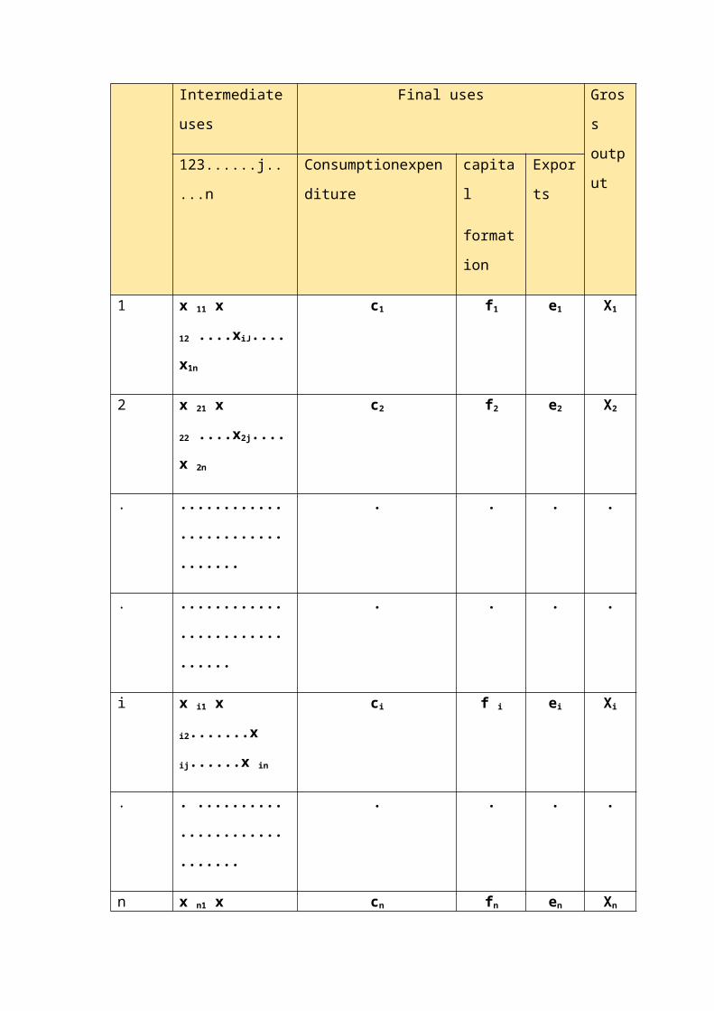
Table 20: Backward and Forward linkages

Backward linkages Forward linkages

input coefficients (A) Output coefficients (B)

Agr Ind Serv Agr Ind Serv Total

1. Agriculture 0.1110 0.0778 0.0264 1. Agriculture 0.1110 0.1239 0.0614 0.2963

2. Industry 0.0505 0.3052 0.1355 2. Industry 0.0317 0.3052 0.1982 0.5352

3. Services 0.0789 0.2232 0.1943 3. Services 0.0339 0.1526 0.1943 0.3808

Products 0.2404 0.6063 0.3562

Leontief matrix (I-A) Leontief matrix (I-B)

1. Agriculture 0.8890 -0.0778 -0.0264 1. Agriculture 0.8890 -0.1239 -0.0614 0.7037

2. Industry -0.0505 0.6948 -0.1355 2. Industry -0.0317 0.6948 -0.1982 0.4648

3. Services -0.0789 -0.2232 0.8057 3. Services -0.0339 -0.1526 0.8057 0.6192

Products 0.7596 0.3937 0.6438

Leontief inverse matrix (I-A)-1 Leontief inverse matrix (I-B)-1

1. Agriculture 1.1387 0.1475 0.0621 1. Agriculture 1.1387 0.2348 0.1445 1.5180

2. Industry 0.1105 1.5359 0.2619 2. Industry 0.0694 1.5359 0.3832 1.9885

3. Services 0.1422 0.4400 1.3199 3. Services 0.0611 0.3008 1.3199 1.6817

Products 1.3914 2.1234 1.6439

46. In its simplest form, the strength of the backward linkage of a sector j is given by the

column sum of the direct input coefficients. A more useful and comprehensive measure

is provided by the column sums of the inverse, which reflects the direct and indirect

effects. From Table 35, the sector industry has the most profound backward linkages (bj

= 2.1234). Backward linkages are demand-oriented. The sector industry requires inputs

from many other sectors. Thus, strong backward linkages must be expected for this

sector. Forward linkages are supply oriented. The sector industry supplies goods to all

other sectors. This sector is expected to have strong forward linkages (many clients). In

the case of agriculture, the forward linkages (1.5180) are higher than backward linkages

(1.3914).

Links between the three quadrants of I-O table47. The I-O table has three quadrants which represent (ii) inter-industry supplies/inputs, (ii)

final demand and (iii) primary inputs. With the help of I-O models, it is possible to

establish links between:

final demand and domestic output in which entire domestic output is expressed in

terms of final demand categories by sectors. This means the intermediate supplies part

of sectoral domestic outputs are transferred to final demand categories. Therefore, the

sum of final demand categories adds upto domestic output. The difference between the

table on total domestic production attributed to final demand (both direct and indirect)

and final demand (direct) represents the indirect effect.

Primary inputs and domestic output, in which the entire domestic output is ascribed to

primary inputs. In other words, this means all the intermediate goods and services are

transferred to primary inputs. Here, the sum of primary inputs equals the domestic

output.

Primary inputs and final demand, in which the final demand by product (sectors) and

by category (consumption expenditure, capital formation and exports) are expressed in

terms of primary inputs. The sum of primary inputs equals the domestic part of final

demand.

Link between final demand and industrial output levels48. The direct link between final demand and industrial output describes the deliveries of

finished goods and services to the various final demand categories. It does not take into

account the intermediate outputs, i.e. raw materials and semi-finished goods which are

required to produce finished goods. These intermediates represent the indirect links

between final demand and output levels. The direct and indirect link can be identified

by multiplying the Leontief Inverse with the matrix of final demand categories ((I-A)-1 *

Y). The resulting matrix shows the industrial output levels directly and indirectly

necessary to meet the final demand requirements. In other words, it indicates the total

importance of each category of final demand for the production of different product

groups. In this compilation, all intermediate consumption part of the domestic output is

transferred to the final demand by using Leontief Inverse. Table 36 shows the direct and

indirect final demand requirements in percentage terms for the domestic output and the

actual distribution in value terms of final demand vectors in the domestic output in

different formats.

Table 21: Total industrial production attributed to final demand

X HFCE GFCE GCF FU Output

FINAL DEMAND (Y)

1. Agriculture 53 2055 14 25 2146 3050

2. Industry 415 1028 105 707 2256 4853

3. Services 267 2350 767 1011 4395 7099

Total 734 5434 886 1743 8798 15002

Shares in domestic production (Direct production attributed to final demand)

1. Agriculture 1.72 67.38 0.45 0.82 70.37

2. Industry 8.55 21.19 2.17 14.57 46.48

3. Services 3.75 33.11 10.81 14.24 61.92

Total 4.89 36.22 5.91 11.62 58.64

OUTPUT (domestic output in FD) = (I-A)-1 * Y

1. Agriculture 138 2638 79 195 3050

2. Industry 713 2422 364 1354 4853

3. Services 542 3847 1061 1649 7099

total 1393 8907 1504 3198 15002

Dependencies of domestic production on final demand (%) (Direct and indirect production

attributed to final use)

1. Agriculture 4.51 86.49 2.59 6.41 100.00

2. Industry 14.69 49.91 7.50 27.89 100.00

3. Services 7.63 54.19 14.95 23.23 100.00

total 9.28 59.37 10.03 21.32 100.00

Intermediate inputs transferred to final demand (indirect production attributed to final use)

1. Agriculture 2.79 19.11 2.13 5.59 29.63

2. Industry 6.14 28.72 5.34 13.32 53.52

3. Services 3.88 21.08 4.14 8.99 38.08

total 4.39 23.15 4.12 9.70 41.36

49. This table shows total (direct and indirect) production (15002) that is attributed to final

demand (8798) in value terms and in percentages illustrating the total (direct and

indirect) dependency of product groups on final demand. The last column represents

total output of product groups. This is caused by the fact that all intermediate outputs

are “transferred” to final demand because of the use of the Leontief Inverse. In this

example, direct share of industry (46.48%) is lower than the indirect share (53.52%), as

the intermediate consumption indirectly attributed to final use of industrial products is

much higher.

Link between domestic output and primary inputs50. The input structure of product groups is composed of intermediate inputs and primary

inputs. But intermediate inputs must also be produced before they are delivered to the

next stage of production. In the corresponding production process not only raw

materials are used but also primary inputs are needed. Therefore, it is possible to ascribe

all intermediate goods and services to the primary inputs required. The interrelation

between primary inputs and one unit of production induced by final demand can be

disclosed by multiplying the primary input coefficients with the Leontief Inverse. The

resulting matrix depicts how many primary inputs are directly and indirectly used within

the whole production process in order to satisfy one unit of final demand for goods and

services j. Due to the fact that the intermediate inputs are “converted” into primary

inputs, the total input coefficients for primary inputs per unit of production add up to

one.

Table 22: Total industrial production attributed to primary inputs

Direct & indirect primary inputs for one unit of final demand (primary input coefficients *

Leontief inverse)

Agr Ind Serv

Taxes less subsidies on products (TLS) 0.0190 0.0610 0.0352

Imported goods and services (M) 0.0245 0.0946 0.0472

Compensation of employees 0.4020 0.3993 0.4406

Other taxes less subsidies on production 0.0000 0.0000 0.0000

Consumption of fixed capital 0.0941 0.0829 0.0913

Net operating surplus 0.4604 0.3623 0.3858

Gross value added at basic prices 0.9564 0.8444 0.9176

Primary inputs (M+TLS+GVA) 1.0000 1.0000 1.0000

Direct primary inputs for one unit of final demand (from matrix A)









Indirect primary inputs for one unit of final demand









51. This table shows that compensation of employees in industries have an input coefficient

of 0.1478, but the coefficient when indirect inputs (intermediate consumption part

transferred to compensation of employees, which in this case is 0.2515) are added, the

input coefficient becomes 0.3933. This also means that of the total output, as much as

0.3993 is accounted by compensation of employees either directly or indirectly.

Links between primary inputs and final demand52. The multipliers in Table 37 allow assessing the primary input content of final demand

by product and by category. The results are presented in Table 38 for the primary input

content of final demand by product and in Table 39 for the primary input content of

final demand by category.

Table 23: Primary input content of final demand by product

(Table 37 * FD row in Table 38)

Direct & indirect primary inputs for one unit of final demand (primary input coefficients *

Leontief inverse)

Agriculture Industry Services Total

Final Demand (Transpose of FD,

Table-9) 2146 2256 4395 8798

Direct and indirect primary inputs for one unit of final demand

Taxes less subsidies on products (TLS) 41 138 155 333

Imported goods and services (M) 53 213 208 474

Compensation of employees 863 901 1937 3700

Other taxes less subsidies on

production 0 0 0 0

Consumption of fixed capital 202 187 401 790

Net operating surplus 988 817 1696 3501

GVA at basic prices 2053 1905 4033 7991

Primary inputs (M+TLS+GVA) 2146 2256 4395 8798

Direct primary inputs for one unit of final demand

Taxes less subsidies on products

(TLS) 24 74 86 184




production 0 0 0 0





Indirect primary inputs for one unit of final demand


(TLS) 17 63 69 149




production 0 0 0 0





Final demand vector is the transpose of final demand vector shown in I-O Table (Table 24);

Other entries are computed as FD (row 1) * Table 37

By categories53. The multipliers for primary inputs [B (I-A)-1] (B is input coefficients for primary inputs)

are multiplied with a matrix of final demand by category to assess the direct and indirect

primary input requirements for the various categories of final demand (consumption,

investment, exports). In Table 39, the entire final demand of domestic output is

transferred to primary inputs, showing the direct and indirect contribution of each of the

primary inputs in each of the final demand components. In the I-O table, there is no

link between final demand components and the value added components. From Table

39, it is possible to see that household consumption of 5434 has an indirect component

of 2272 of compensation of employees. Exports too indirectly account for 304 of

compensation of employees out of 734.

Table 24: Primary input content of final demand by category

X HFCE GFCE GCF FU

Final demand 734 5434 886 1743 8798

domestic production = B*(I-A)-1*Y

Agriculture 85 583 65 171 904

Industry 298 1394 259 647 2597

Services 275 1496 294 638 2704

DOMESTIC 658 3473 618 1455 6204

Primary input of final demand = B*(I-A)-1*Y


(TLS) 36 185 34 79 333

Imported goods and services (M) 53 259 47 115 474

Supply = B*(I-A)-1*Y

Total 747 3916 698 1650 7011

Income = B*(I-A)-1*Y

Compensation of employees 304 2272 386 738 3700


production0 0 0 0

0

Consumption of fixed capital 64 493 80 153 790

Net operating surplus 277 2225 341 658 3501

GVA at basic prices 645 4991 806 1549 7991

Primary inputs (M+TLS+GVA) 734 5434 886 1743 8798

B: input coefficients (Table 28); (I-A)-1*Y is the total output represented by FD (Table 36)

(b) Examples for multiplier and impact analysis

54. The above economic analyses are based on linkages within the input-output table. But

the modelling approaches presented for diagnostic purposes can also be applied for

impact analysis. In that case exogenous variables will be combined with the Leontief

Inverse of the input-output model assuming the stability of coefficients for the change to

be analysed. The following few examples demonstrate the effects of a change in final

demand or primary inputs on the input-output system in the economy.

(i) Based on quantity modelsImpact on domestic output by increasing the gross capital formation of ‘industry’

55. From Table 24, we can see that of the total uses of ‘industry’ sector output of 4853, 707

goes to gross capital formation. Suppose we increase this GCF by 100%, i.e. 707 and

want to see the impact on the domestic output of the economy. The output can be

estimated by the I-O model (I-A)-1*y. The impact analysis is demonstrated in Table 40.

From this table, it is seen that increase of 707 in GCF from ‘industry’ induces total

production of 1501 of which direct production effect is 707 and indirect production

effect is 794. This includes 379 in ‘industry’, 104 in ‘agriculture’ and 311 in ‘services’.

Table 25: Direct and indirect effects on domestic production induced by 100%

increase in GCF from ‘Industry’ sector

Agr Ind Serv

*

FD*

=

Output Indirect effect

1. Agriculture 1.1387 0.1475 0.0621 0 104 104

2. Industry 0.1105 1.5359 0.2619 707 1086 379

3. Services 0.1422 0.4400 1.3199 0 311 311

Total 1.3914 2.1234 1.6439 707 1501 794

*FD here is increase in GCF of industry, and this is also the direct effect. The inter-industry figures are

Leontief inverse.

Impact on domestic output by increasing HFCE of ‘services’

56. Another example is increase in HFCE in respect of ‘services’. From Table 24, it can be

seen that as much as 2350 of 7099 of output of ‘services’ is HFCE. Suppose we raise

this consumption expenditure by 10% and would like to see the total impact on

domestic output on account of this increase. Table 41 shows that direct increase is 235

but this will induce an indirect effect of 151 on the domestic output. This increase can

be seen in all sectors, but the maximum indirect effect is in ‘services’ (75), and

‘industry’ (62). This implies other sectors too require to raise their output levels to meet

the induced demand of 10% extra HFCE of ‘services’, due to inter-industry linkages.

Table 26: Direct and indirect effects on domestic production induced by 10%

increase in HFCE of ‘services’

Agr Ind Serv

*

FU

=

Output Indirect effect

1. Agriculture 1.13870.147

50.0621

0 15 15

2. Industry 0.11051.535

90.2619

0 62 62

3. Services 0.14220.440

01.3199

235 310 75

Total 1.39142.123

41.6439 235 386

151

*FD here is increase in CE of ‘other services’, and this is also the direct effect. The inter-industry

figures are Leontief inverse.

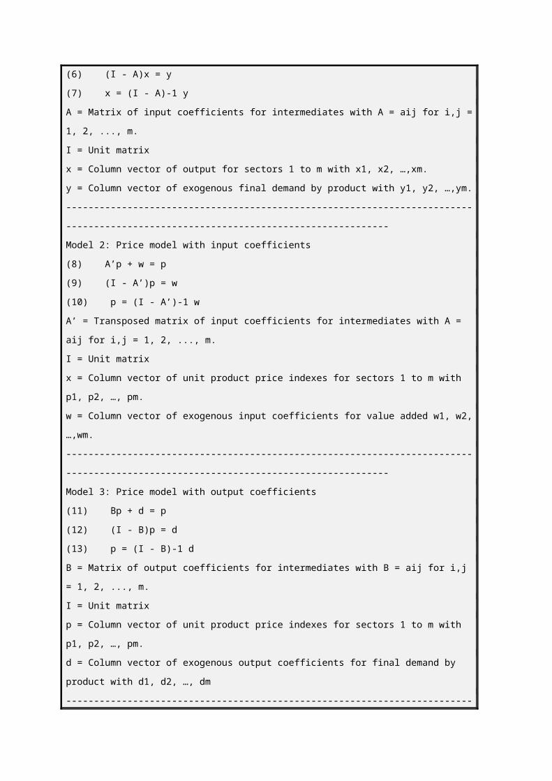
(ii) Based on price modelsPrice increases of primary inputs induce inflation

57. Price increases of primary inputs (imports, capital, and labour) threaten the price

stability in many countries. In the following calculation it is assumed that the prices of

all primary inputs increase in agriculture, forestry & fishing and industry. In Table 42,

the impact on product prices has been calculated with the price model of input-output

analysis. One fundamental feature of the price model is the assumption that firms have

the market power to fully reflect rising costs of primary inputs in their product prices.

Table 27: Price increase of 10% in primary inputs of agriculture and industry

Agr Ind Serv

input

coefficient

for primary

inputs

Price

Index

new input

coefficient for

primary inputs

Price

Index

1. Agriculture 1.1387 0.1105 0.1422 0.7596 1.0000 0.8356 1.09085

2. Industry 0.1475 1.5359 0.4400 0.3937 1.0000 0.4331 1.07168

3. Services 0.0621 0.2619 1.3199 0.6438 1.0000 0.6438 1.01503

The inter-industry matrix is transpose of Leontief inverse and the column of input coefficient for primary

inputs is the transpose of input coefficients for primary inputs from the input coefficient matrix

Table 28: Impact of 10% price increases in primary inputs of Agriculture and Industry

Old HFCE New HFCE Growth rate

1. Agriculture 2055 2242 9.1

2. Industry 1028 1102 7.2

3. Services 2350 2386 1.5

Total 5434 5730 5.4

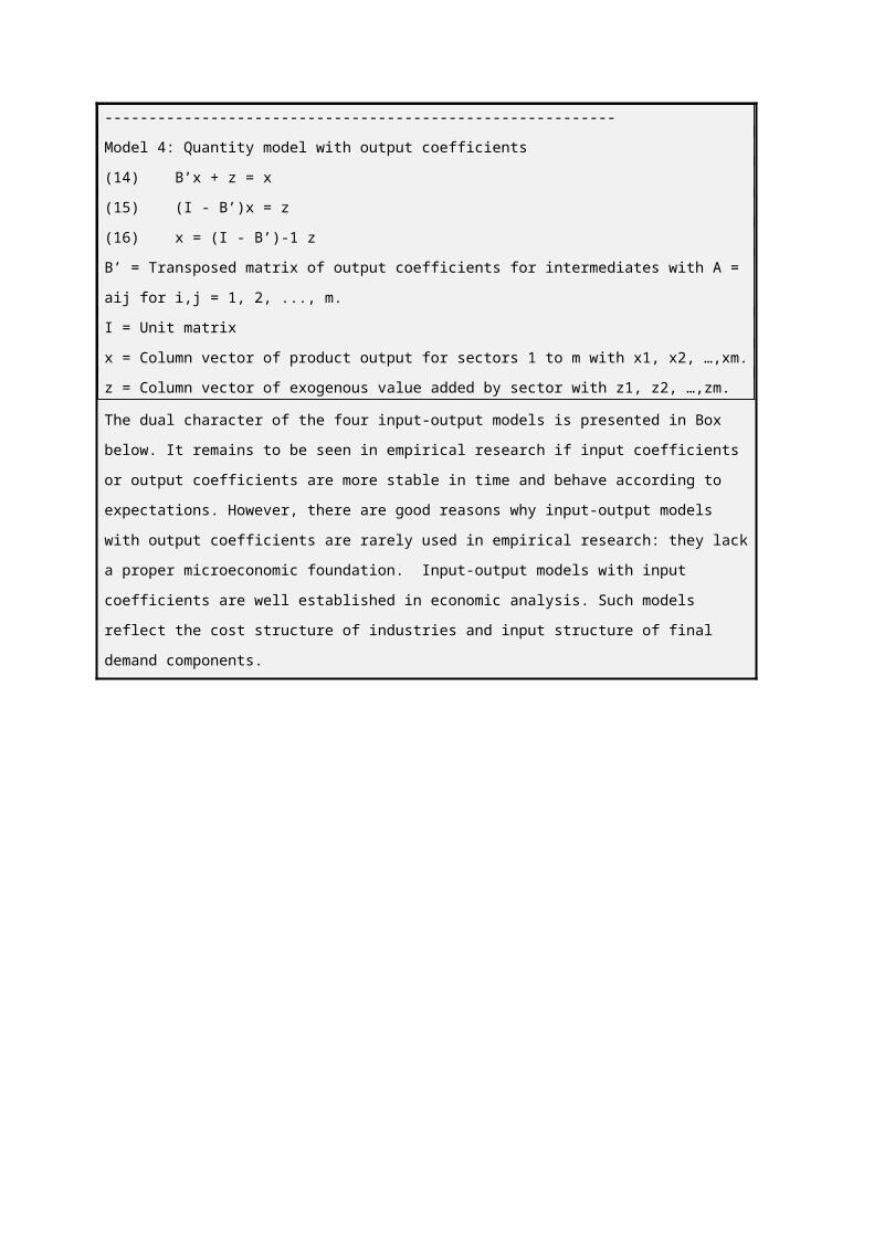
58. If prices for primary inputs in agriculture and industry increase by 10 %, it is expected

that the prices of agriculture and industry goods will increase by 9.1 %, and 7.2%

respectively. Prices of services will go up by 1.5%. Taking the consumption

expenditure of households as the weighting diagram for CPI, the overall price rise will

be 5.4%.

(c) Input-output models with endogenous final demand

59. In the usual form of the standard demand-side input-output model, the final demand

elements are considered exogenous. However, private consumption and investment in

many respects depend on income. The basic idea of introducing more endogenous

variables is to separate the components of final demand into autonomous and variable

elements. For the remaining components of final demand (government consumption,

exports) it does not seem to be feasible to treat them in a corresponding way as

endogenous variables.

60. In the previous analysis, private consumption and consequently household activities are

exogenous. A more refined income multiplier analysis for wages tries to include the

household sector as an endogenous activity. The income earned by private households is

spent to a large extent for private consumption. This induces higher incomes, which

again induces more private consumption.

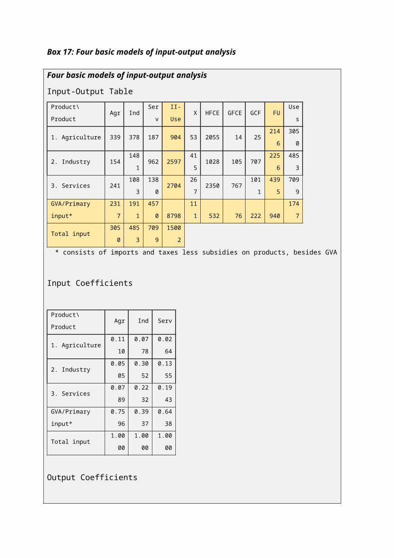
Table 29: Income multiplier for wages with endogenous private consumption

Agriculture Industry Service HFCE

INPUT COEFFICIENTS (A)

1. Agriculture 0.1110 0.0778 0.0264 0.5554

2. Industry 0.0505 0.3052 0.1355 0.2779

3. Services 0.0789 0.2232 0.1943 0.6352

7.1 COE 0.3024 0.1478 0.2902 0.0000

(I-A)

1. Agriculture 0.8890 -0.0778 -0.0264 -0.5554

2. Industry -0.0505 0.6948 -0.1355 -0.2779

3. Services -0.0789 -0.2232 0.8057 -0.6352

7.1 COE -0.3024 -0.1478 -0.2902 1.0000

Inverse (I-A)-1

1. Agriculture 1.8814 0.8853 0.8761 1.84763

2. Industry 0.7924 2.2132 1.0093 1.69644

3. Services 1.2252 1.5157 2.5069 2.69429

7.1 COE 1.0417 1.0347 1.1417 2.59147

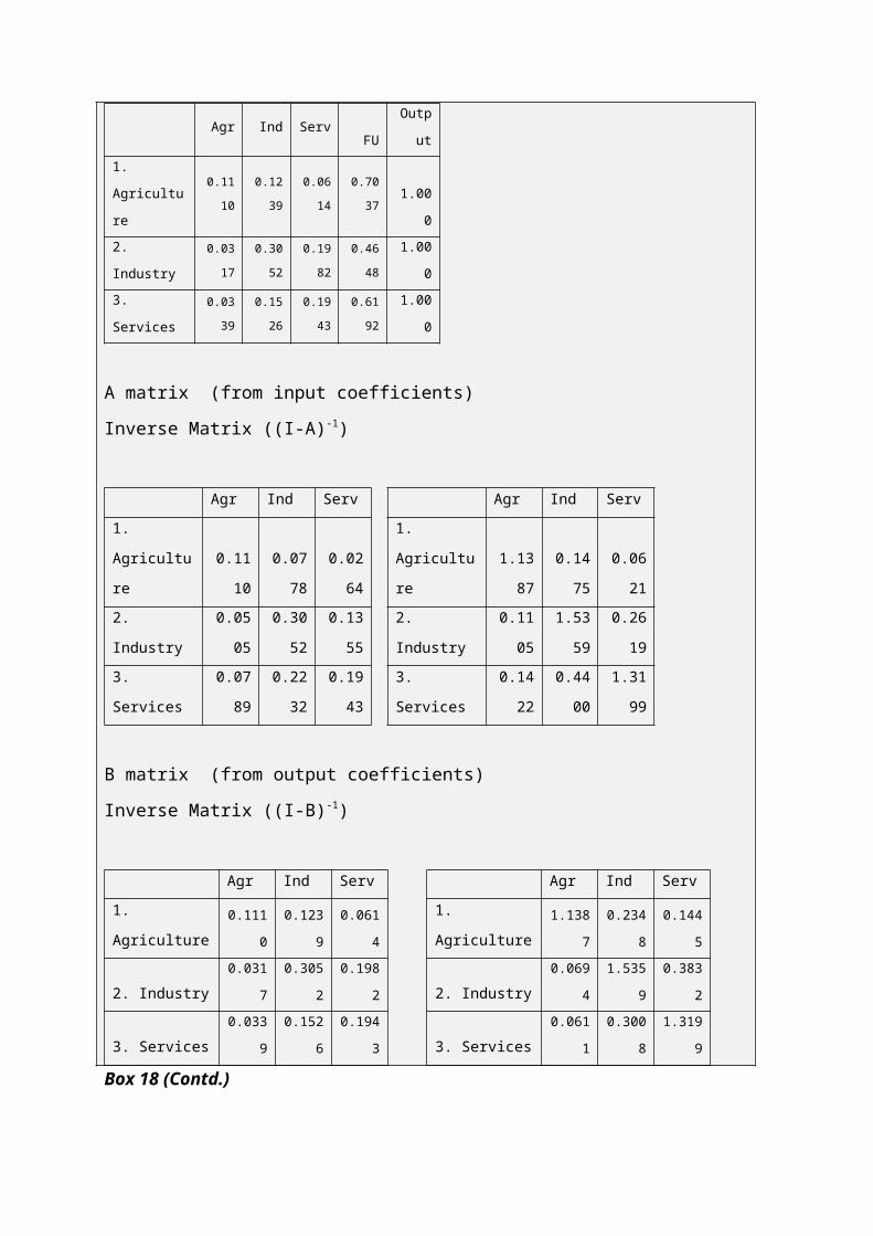
Table 30: Quantity model with endogenous private consumption

Agr. Ind. Service HFCE

*

FD

=

Output

1. Agriculture 1.8814 0.8853 0.8761 1.84763 91 3050

2. Industry 0.7924 2.2132 1.0093 1.69644 1227 4853

3. Services 1.2252 1.5157 2.5069 2.69429 2045 7099

7.1 COE 1.0417 1.0347 1.1417 2.59147 0 3700

61. The above tables present the I-O model with HFCE and compensation of employees as

endogenous variables.The wage multiplier with exogenous private consumption for

agriculture was 0.4020 (see Table 37). If private consumption and wages and salaries

are treated as endogenous variables, the wage multiplier rises to 1.0417, in the last row

of Table 45. The high multiplier in this case as compared to the multipliers when HFCE

was treated as exogenous variable is due to very high proportion of HFCE and

compensation of employees in final demand.

References

EUROSTAT 2008. Eurostat Manual of Supply, Use and Input-Output Tables. Luxembourg

United Nations,1999. Handbook of Input-Output Tables: Compilation and Analysis, Studies in Methods, Series F, Number 74, New York

Documents

EN/SUT/2014/Doc/1 - ECAStats: Online accessecastats.uneca.org/acsweb/Portals/0/Economic Statistics... · Web view2369 6678 804 5707 913 1867 967 8324 15002 5. TLS-prod 33 177 123