Ensemble Approaches for Regression: a

Survey

Joao M. Moreira a,∗, Carlos Soares b,c, Alıpio M. Jorge b,c andJorge Freire de Sousa a

aFaculty of Engineering, University of Porto, Rua Dr. Roberto Frias, s/n4200-465 Porto PORTUGAL

bFaculty of Economics, University of Porto, Rua Dr. Roberto Frias, s/n4200-464 Porto PORTUGAL

cLIAAD, INESC Porto L.A., R. de Ceuta, 118, 6, 4050-190, Porto PORTUGAL

Abstract

This paper discusses approaches from different research areas to ensemble regression.The goal of ensemble regression is to combine several models in order to improvethe prediction accuracy on learning problems with a numerical target variable. Theprocess of ensemble learning for regression can be divided into three phases: thegeneration phase, in which a set of candidate models is induced, the pruning phase,to select of a subset of those models and the integration phase, in which the outputof the models is combined to generate a prediction. We discuss different approachesto each of these phases, categorizing them in terms of relevant characteristics andrelating contributions from different fields. Given that previous surveys have focusedon classification, we expect that this work will provide a useful overview of existingwork on ensemble regression and enable the identification of interesting lines forfurther research.

Key words: ensembles, regression, supervised learning

1 Introduction

Ensemble learning typically refers to methods that generate several modelswhich are combined to make a prediction, either in classification or regression

∗ Tel.: +351225081639; fax: +351225081538Email address: jmoreira@fe.up.pt (Joao M. Moreira).

Preprint submitted to Elsevier 19 December 2007

problems. This approach has been the object of a significant amount of re-search in recent years and good results have been reported (e.g., [1–3]). Theadvantage of ensembles with respect to single models has been reported interms of increased robustness and accuracy [4].

Most work on ensemble learning focuses on classification problems. However,techniques that are successful for classification are often not directly appli-cable for regression. Therefore, although both are related, ensemble learningapproaches have been developed somehow independently. Therefore, existingsurveys on ensemble methods for classification [5,6] are not suitable to providean overview of existing approaches for regression.

This paper surveys existing approaches to ensemble learning for regression.The relevance of this paper is strengthened by the fact that ensemble learningis an object of research in different communities, including pattern recog-nition, machine learning, statistics and neural networks. These communitieshave different conferences and journals and often use different terminology andnotation, which makes it quite hard for a researcher to be aware of all contri-butions that are relevant to his/her own work. Therefore, besides attemptingto provide a thorough account of the work in the area, we also organize thoseapproaches independently of the research area they were originally proposedin. Hopefully, this organization will enable the identification of opportunitiesfor further research and facilitate the classification of new approaches.

In the next section, we provide a general discussion of the process of ensem-ble learning. This discussion will lay out the basis according to which theremaining sections of the paper will be presented: ensemble generation (Sect.3), ensemble pruning (Sect. 4) and ensemble integration (Sect. 5). Sect. 6concludes the paper with a summary.

2 Ensemble Learning for Regression

In this section we provide a more accurate definition of ensemble learningand provide terminology. Additionally, we present a general description of theprocess of ensemble learning and describe a taxonomy of different approaches,both of which define the structure of the rest of the paper. Next we discussthe experimental setup for ensemble learning. Finally, we analyze the errordecompositon of ensemble learning methods for regression.

2

2.1 Definition

First of all we need to define clearly what ensemble learning is, and to define ataxonomy of methods. As far as we know, there is no widely accepted definitionof ensemble learning. Some of the existing definitions are partial in the sensethat they focus just on the classification problem or on part of the ensemblelearning process [7]. For these reasons we propose the following definition:

Definition 1 Ensemble learning is a process that uses a set of models, eachof them obtained by applying a learning process to a given problem. This setof models (ensemble) is integrated in some way to obtain the final prediction.

This definition has important characteristics. In the first place, contrary tothe informal definition given at the beginning of the paper, this one coversnot only ensembles in supervised learning (both classification and regressionproblems), but also in unsupervised learning, namely the emerging researcharea of ensembles of clusters [8].

Additionally, it clearly separates ensemble and divide-and-conquer approaches.This last family of approaches split the input space in several sub-regionsand train separately each model in each one of the sub-regions. With thisapproach the initial problem is converted in the resolution of several simplersub-problems.

Finally, it does not separate the combination and selection approaches as itis usually done. According to this definition, selection is a special case ofcombination where the weights are all zero except for one of them (to bediscussed in Sect. 5).

More formally, an ensemble F is composed of a set of predictors of a functionf denoted as fi.

F = {fi, i = 1, ..., k}. (1)

The resulting ensemble predictor is denoted as ff .

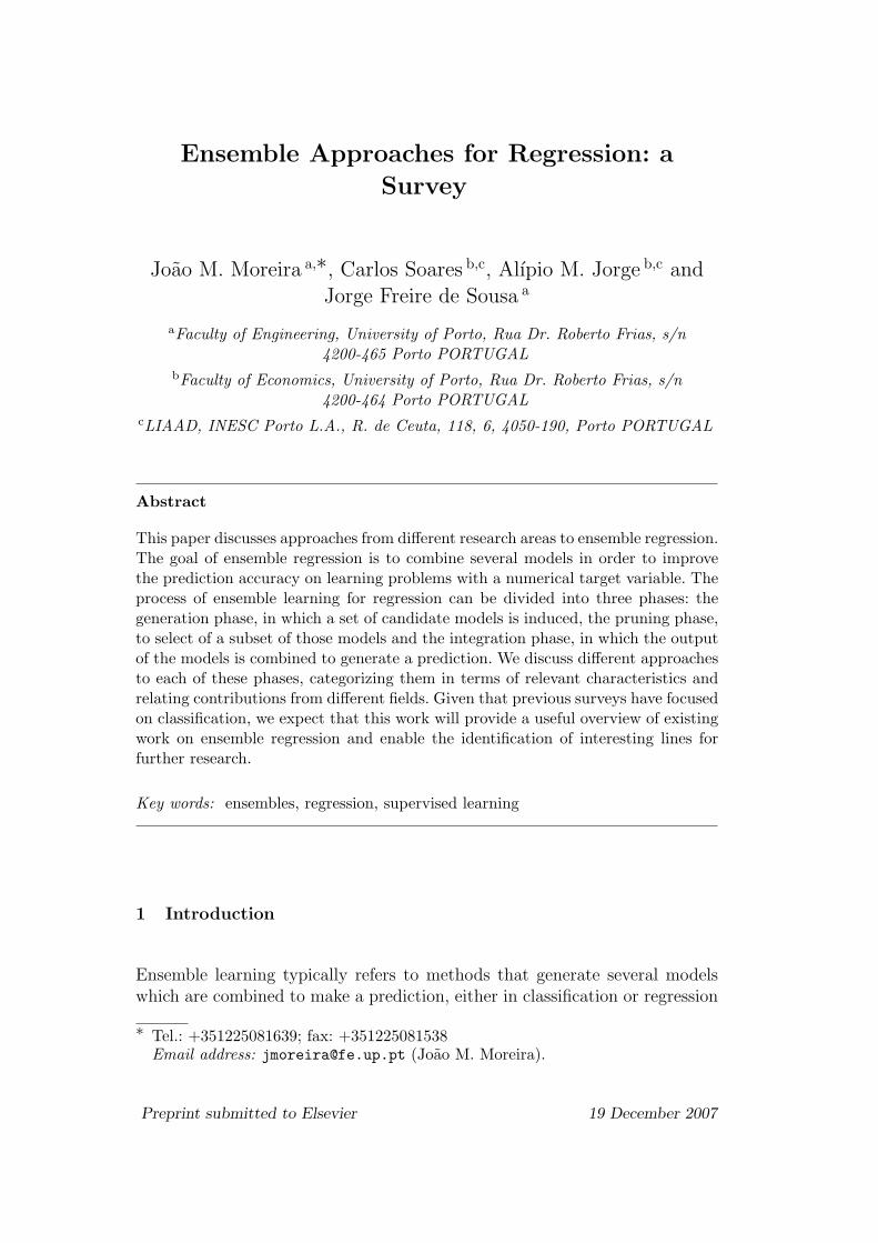
2.1.1 The Ensemble Learning Process

The ensemble process can be divided into three steps [9] (Fig. 1), usuallyreferred as the overproduce-and-choose approach. The first step is ensemblegeneration, which consists of generating a set of models. It often happensthat, during the first step, a number of redundant models are generated. Inthe ensemble pruning step, the ensemble is pruned by eliminating some of themodels generated earlier. Finally, in the ensemble integration step, a strategy

3

to combine the base models is defined. This strategy is then used to obtainthe prediction of the ensemble for new cases, based on the predictions of thebase models.

Generation Pruning Integration

Fig. 1. Ensemble learning model

Our characterization of the ensemble learning process is slightly more detailedthan the one presented by Rooney et al. [10]. For those authors, ensemblelearning consists on the solution of two problems: (1) how to generate theensemble of models? (ensemble generation); and (2) how to integrate the pre-dictions of the models from the ensemble in order to obtain the final ensembleprediction? (ensemble integration). This last approach (without the pruningstep), is named direct, and can be seen as a particular case of the modelpresented in Fig. 1, named overproduce-and-choose.

Ensemble pruning has been reported, at least in some cases, to reduce the sizeof the ensembles obtained without degrading the accuracy. Pruning has alsobeen added to direct methods successfully increasing the accuracy [11,12]. Asubject to be discussed further in Sect. 4.

2.1.2 Taxonomy and Terminology

Concerning the categorization of the different approaches to ensemble learning,we will follow mainly the taxonomy presented by the same authors [10]. Theydivide ensemble generation approaches into homogeneous , if all the modelswere generated using the same induction algorithm, and heterogeneous , oth-erwise.

Ensemble integration methods, are classified by some authors [10,13] as com-bination (also called fusion) or as selection. The former approach combinesthe predictions of the models from the ensemble in order to obtain the finalensemble prediction. The latter approach selects from the ensemble the mostpromising model(s) and the prediction of the ensemble is based on the se-lected model(s) only. Here, we use, instead, the classification of constant vs.non-constant weighting functions given by Merz [14]. In the first case, thepredictions of the base models are always combined in the same way. In thesecond case, the way the predictions are combined can be different for differentinput values.

As mentioned earlier, research on ensemble learning is carried out in differentcommunities. Therefore, different terms are sometimes used for the same con-cept. In Table 1 we list several groups of synonyms, extended from a previouslist by Kuncheva [5]. The first column contains the most frequently used termsin this paper.

4

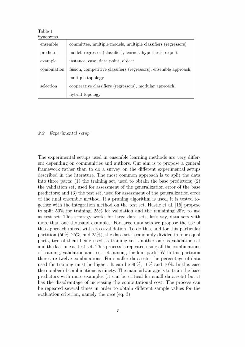
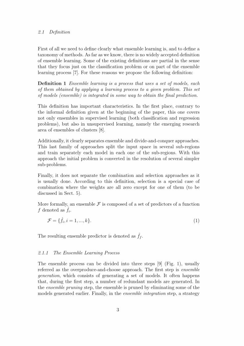
Table 1Synonyms

ensemble committee, multiple models, multiple classifiers (regressors)

predictor model, regressor (classifier), learner, hypothesis, expert

example instance, case, data point, object

combination fusion, competitive classifiers (regressors), ensemble approach,

multiple topology

selection cooperative classifiers (regressors), modular approach,

hybrid topology

2.2 Experimental setup

The experimental setups used in ensemble learning methods are very differ-ent depending on communities and authors. Our aim is to propose a generalframework rather than to do a survey on the different experimental setupsdescribed in the literature. The most common approach is to split the datainto three parts: (1) the training set, used to obtain the base predictors; (2)the validation set, used for assessment of the generalization error of the basepredictors; and (3) the test set, used for assessment of the generalization errorof the final ensemble method. If a pruning algorithm is used, it is tested to-gether with the integration method on the test set. Hastie et al. [15] proposeto split 50% for training, 25% for validation and the remaining 25% to useas test set. This strategy works for large data sets, let’s say, data sets withmore than one thousand examples. For large data sets we propose the use ofthis approach mixed with cross-validation. To do this, and for this particularpartition (50%, 25%, and 25%), the data set is randomly divided in four equalparts, two of them being used as training set, another one as validation setand the last one as test set. This process is repeated using all the combinationsof training, validation and test sets among the four parts. With this partitionthere are twelve combinations. For smaller data sets, the percentage of dataused for training must be higher. It can be 80%, 10% and 10%. In this casethe number of combinations is ninety. The main advantage is to train the basepredictors with more examples (it can be critical for small data sets) but ithas the disadvantage of increasing the computational cost. The process canbe repeated several times in order to obtain different sample values for theevaluation criterion, namely the mse (eq. 3).

5

2.3 Regression

In this paper we assume a typical regression problem. Data consists of a set ofn examples of the form {(x1, f (x1)) , . . . , (xn, f (xn))}. The goal is to inducea function f from the data, where

f : X → <, where, f(x) = f(x),∀x ∈ X, (2)

where f represents the unknown true function. The algorithm used to obtainthe f function is called induction algorithm or learner. The f function is calledmodel or predictor. The usual goal for regression is to minimize a squared errorloss function, namely the mean squared error (mse),

mse =1

n

n∑

i

(f(xi)− f(xi))2. (3)

2.4 Understanding the generalization error of ensembles

To accomplish the task of ensemble generation, it is necessary to know thecharacteristics that the ensemble should have. Empirically, it is stated byseveral authors that a good ensemble is the one with accurate predictors andmaking errors in different parts of the input space. For the regression problemit is possible to decompose the generalization error in different components,which can guide the process to optimize the ensemble generation.

Here, the functions are represented, when appropriate, without the input vari-ables, just for the sake of simplicity. For example, instead of f(x) we use f .We closely follow Brown [16].

Understanding the ensemble generalization error enables us to know whichcharacteristics should the ensemble members have in order to reduce the over-all generalization error. The generalization error decomposition for regressionis straightforward. What follows is about the decomposition of the mse (eq.3). Despite the fact that the majority of the works were presented in the con-text of neural network ensembles, the results presented in this section are notdependent of the induction algorithm used.

Geman et al. present the bias/variance decomposition for a single neural net-work [17]:

E{[f − E(f)]2} = [E(f)− E(f)]2 + E{[f − E(f)]2}. (4)

The first term on the right hand side is called the bias and represents the

6

distance between the expected value of the estimator f and the unknown pop-ulation average. The second term, the variance component, measures how thepredictions vary with respect to the average prediction. This can be rewrittenas:

mse(f) = bias(f)2 + var(f). (5)

Krogh & Vedelsby describe the ambiguity decomposition, for an ensemble ofk neural networks [18]. Assuming that ff (x) =

∑ki=1[αi× fi(x)] (see Sect. 5.1)

where∑k

i=1(αi) = 1 and αi ≥ 0, i = 1, ..., k, they show that the error for asingle example is:

(ff − f)2 =k∑

i=1

[αi × (fi − f)2]−k∑

i=1

[αi × (fi − ff )2]. (6)

This expression shows explicitly that the ensemble generalization error is lessthan or equal to the generalization error of a randomly selected single predic-tor. This is true because the ambiguity component (the second term on theright) is always non negative. Another important result of this decompositionis that it is possible to reduce the ensemble generalization error by increasingthe ambiguity without increasing the bias. The ambiguity term measures thedisagreement among the base predictors on a given input x (omitted in theformulae just for the sake of simplicity, as previously referred). Two full proofsof the ambiguity decomposition [18] are presented in [16].

Later, Ueda & Nakano presented the bias/variance/covariance decompositionof the generalization error of ensemble estimators [19]. In this decompositionit is assumed that ff (x) = 1

k×∑k

i=1[fi(x)]:

E[(ff − f)2] = bias2+

1

k× var + (1− 1

k)× covar, (7)

where

bias =1

k×

k∑

i=1

[Ei(fi)− f ], (8)

var =1

k×

k∑

i=1

{Ei{[fi − Ei(fi)]2}}, (9)

covar =1

k × (k − 1)×

k∑

i=1

k∑

j=1,j 6=i

Ei,j{[fi − Ei(fi)][fj − Ej(fj)]} . (10)

7

The indexes i, j of the expectation mean that the expression is true for par-ticular training sets, respectively, Li and Lj.

Brown provides a good discussion on the relation between ambiguity and co-variance [16]. An important result obtained from the study of this relation isthe confirmation that it is not possible to maximize the ensemble ambiguitywithout affecting the ensemble bias component as well, i.e., it is not possi-ble to maximize the ambiguity component and minimize the bias componentsimultaneously.

The discussion of the present section is usually referred in the context ofensemble diversity, i.e., the study on the degree of disagreement between thebase predictors. Many of the above statements are related to the well knownstatistical problem of point estimation. This discussion is also related with themulti-collinearity problem that will be discussed in Sect. 5.

3 Ensemble generation

The goal of ensemble generation is to generate a set of models, F = {fi, i =1, ..., k}. If the models are generated using the same induction algorithm theensemble is called homogeneous, otherwise it is called heterogeneous.

Homogeneous ensemble generation is the best covered area of ensemble learn-ing in the literature. See, for example, the state of the art surveys from Di-etterich [7], or Brown et al. [20]. In this section we mainly follow the former[7]. In homogeneous ensembles, the models are generated using the same algo-rithm. Thus, as explained in the following sections, diversity can be achievedby manipulating the data (Section 3.1) or by the model generation process(Section 3.2).

Heterogeneous ensembles are obtained when more than one learning algorithmis used. This approach is expected to obtain models with higher diversity [21].The problem is the lack of control on the diversity of the ensemble duringthe generation phase. In homogeneous ensembles, diversity can be systemati-cally controlled during their generation, as will be discussed in the followingsections. Conversely, when using several algorithms, it may not be so easy tocontrol the differences between the generated models. This difficulty can besolved by the use of the overproduce-and-choose approach. Using this approachthe diversity is guaranteed in the pruning phase [22]. Another approach, com-monly followed, combines the two approaches, by using different inductionalgorithms mixed with the use of different parameter sets [23,10] (Sect. 3.2.1).Some authors claim that the use of heterogeneous ensembles improves theperformance of homogeneous ensemble generation. Note that heterogeneous

8

ensembles can use homogeneous ensemble models as base learners.

3.1 Data manipulation

Data can be manipulated in three different ways: subsampling from the train-ing set, manipulating the input features and manipulating the output targets.

3.1.1 Subsampling from the training set

These methods have in common that the models are obtained using differentsubsamples from the training set. This approach generally assumes that thealgorithm is unstable, i.e., small changes in the training set imply importantchanges in the result. Decision trees, neural networks, rule learning algorithmsand MARS are well known unstable algorithms [24,7]. However, some of themethods based on subsampling (e.g., bagging and boosting) have been suc-cessfully applied to algorithms usually regarded as stable, such as SupportVector Machines (SVM) [25].

One of the most popular of such methods is bagging [26]. It uses randomlygenerated training sets to obtain an ensemble of predictors. If the originaltraining set L has m examples, bagging (bootstrap aggregating) generates amodel by sampling uniformly m examples with replacement (some examplesappear several times while others do not appear at all). Both Breiman [26]and Domingos [27] give insights on why does bagging work.

Based on [28], Freund & Schapire present the AdaBoost (ADAptive BOOST-ing) algorithm, the most popular boosting algorithm [29]. The main idea isthat it is possible to convert a weak learning algorithm into one that achievesarbitrarily high accuracy. A weak learning algorithm is one that performsslightly better than random prediction. This conversion is done by combiningthe estimations of several predictors. Like in bagging [26], the examples arerandomly selected with replacement but, in AdaBoost, each example has adifferent probability of being selected. Initially, this probability is equal for allthe examples, but in the following iterations examples with more inaccuratepredictions have higher probability of being selected. In each new iterationthere are more ’difficult examples’ in the training set. Despite boosting hasbeen originally developed for classification, several algorithms have been pro-posed for regression but none has emerged as being the appropriate one [30].

Parmanto et al. describe the cross-validated committees technique for neuralnetworks ensemble generation using υ-fold cross validation [31]. The main ideais to use as ensemble the models obtained by the use of the υ training sets onthe cross validation process.

9

3.1.2 Manipulating the input features

In this approach, different training sets are obtained by changing the repre-sentation of the examples. A new training set j is generated by replacing theoriginal representation {(xi, f (xi)) into a new one {(x′i, f (xi)) . There are twotypes of approaches. The first one is feature selection, i.e., x′i ⊂ xi. In the sec-ond approach, the representation is obtained by applying some transformationto the original attributes, i.e., x′i = g (xi).

A simple feature selection approach is the random subspace method, consistingof a random selection [32]. The models in the ensemble are independentlyconstructed using a randomly selected feature subset. Originally, decision treeswere used as base learners and the ensemble was called decision forests [32].The final prediction is the combination of the predictions of all the trees inthe forest.

Alternatively, iterative search methods can be used to select the different fea-ture subsets. Opitz uses a genetic algorithm approach that continuously gen-erates new subsets starting from a random feature selection [33]. The authoruses neural networks for the classification problem. He reports better resultsusing this approach than using the popular bagging and AdaBoost methods.In [34] the search method is a wrapper like hill-climbing strategy. The criteriaused to select the feature subsets are the minimization of the individual errorand the maximization of ambiguity (Sect. 2.4).

A feature selection approach can also be used to generate ensembles for al-gorithms that are stable with respect to the training set but unstable w.r.t.the set of features, namely the nearest neighbors induction algorithm. In [35]the feature subset selection is done using adaptive sampling in order to re-duce the risk of discarding discriminating information. Compared to randomfeature selection, this approach reduces diversity between base predictors butincreases their accuracy.

A simple transformation approach is input smearing [36]. It aims to increasethe diversity of the ensemble by adding Gaussian noise to the inputs. Thegoal is to improve the results of bagging. Each input value x is changed intoa smeared value x′ using:

x′ = x + p ∗N(0, σX) (11)

where p is an input parameter of the input smearing algorithm and σX isthe sample standard deviation of X, using the training set data. In this case,the examples are changed, but the training set keeps the same number ofexamples. In this work just the numeric input variables are smeared even ifthe nominal ones could also be smeared using a different strategy. Results

10

compare favorably to bagging. A similar approach called BEN - BootstrapEnsemble with Noise, was previously presented by Raviv & Intrator [37].

Rodriguez et al. [3] present a method that combines selection and transfor-mation, called rotation forests. The original set of features is divided into kdisjoint subsets to increase the chance of obtaining higher diversity. Then, foreach subset, a principal component analysis (PCA) approach is used to projectthe examples into a set of new features, consisting of linear combinations ofthe original ones. Using decision trees as base learners, this strategy assuresdiversity, (decision trees are sensitive to the rotation of the axis) and accuracy(PCA concentrates in a few features most of the information contained in thedata). The authors claim that rotation forests outperform bagging, AdaBoostand random forests (to be discussed further away in Sect. 3.2.2). However, theadaptation of rotation forests for regression does not seem to be straightfor-ward.

3.1.3 Manipulating the output targets

The manipulation of the output targets can also be used to generate differenttraining sets. However, not much research follows this approach and most ofit focus on classification.

An exception is the work of Breiman, called output smearing [38]. The basicidea is to add Gaussian noise to the target variable of the training set, inthe same way as it is done for input features in the input smearing method(Sect. 3.1.2). Using this approach it is possible to generate as many models asdesired. Although it was originally proposed using CART trees as base models,it can be used with other base algorithms. The comparison between outputsmearing and bagging shows a consistent generalization error reduction, evenif not outstanding.

An alternative approach consists of the following steps. First it generates amodel using the original data. Second, it generates a model that estimatesthe error of the predictions of the first model and generates an ensemble thatcombines the prediction of the previous model with the correction of the cur-rent one. Finally, it iteratively generates models that predict the error of thecurrent ensemble and then updates the ensemble with the new model. Thetraining set used to generate the new model in each iteration is obtained byreplacing the output targets with the errors of the current ensemble. This ap-proach was proposed by Breiman, using bagging as the base algorithm andwas called iterated bagging [39]. Iterated bagging reduces generalization errorwhen compared with bagging, mainly due to the bias reduction during theiteration process.

11

3.2 Model generation manipulation

As an alternative to manipulating the training set, it is possible to change themodel generation process. This can be done by using different parameter sets,by manipulating the induction algorithm or by manipulating the resultingmodel.

3.2.1 Manipulating the parameter sets

Each induction algorithm is sensitive to the values of the input parameters.The degree of sensitivity of the induction algorithm is different for differentinput parameters. To maximize the diversity of the models generated, oneshould focus on the parameters which the algorithm is most sensitive to.

Neural network ensemble approaches quite often use different initial weightsto obtain different models. This is done because the resulting models varysignificantly with different initial weights [40]. Several authors, like Rosen, forexample, use randomly generated seeds (initial weights) to obtain differentmodels [41], while other authors mix this strategy with the use of differentnumber of layers and hidden units [42,43].

The k-nearest neighbors ensemble proposed by Yankov et al. [44] has justtwo members. They differ on the number of nearest neighbors used. They areboth sub-optimal. One of them because the number of nearest neighbors istoo small, and the other because it is too large. The purpose is to increasediversity (see Sect. 5.2.1).

3.2.2 Manipulating the induction algorithm

Diversity can be also attained by changing the way induction is done. There-fore, the same learning algorithm may have different results on the same data.Two main categories of approaches for this can be identified: Sequential andparallel. In sequential approaches, the induction of a model is influenced onlyby the previous ones. In parallel approaches it is possible to have more ex-tensive collaboration: (1) each process takes into account the overall qualityof the ensemble and (2) information about the models is exchanged betweenprocesses.

Rosen [41] generates ensembles of neural networks by sequentially trainingnetworks, adding a decorrelation penalty to the error function, to increasediversity. Using this approach, the training of each network tries to minimizea function that has a covariance component, thus decreasing the generalizationerror of the ensemble, as stated in [19]. This was the first approach using the

12

decomposition of the generalization error made by Ueda & Nakano [19] (Sect.2.4) to guide the ensemble generation process. Another sequential method togenerate ensembles of neural networks is called SECA (Stepwise EnsembleConstruction Algorithm) [30]. It uses bagging to obtain the training set foreach neural network. The neural networks are trained sequentially. The processstops when adding another neural network to the current ensemble increasesthe generalization error.

The Cooperative Neural Network Ensembles (CNNE) method [45] also uses asequential approach. In this work, the ensemble begins with two neural net-works and then, iteratively, CNNE tries to minimize the ensemble error firstlyby training the existing networks, then by adding a hidden node to an existingneural network, and finally by adding a new neural network. Like in Rosen’sapproach, the error function includes a term representing the correlation be-tween the models in the ensemble. Therefore, to maximize the diversity, all themodels already generated are trained again at each iteration of the process.The authors test their method not only on classification datasets but also onone regression data set, with promising results.

Tsang et al. [46] propose an adaptation of the CVM (Core Vector Machines)algorithm [47] that maximizes the diversity of the models in the ensemble byguaranteeing that they are orthogonal. This is achieved by adding constraintsto the quadratic programming problem that is solved by the CVM algorithm.This approach can be related to AdaBoost because higher weights are givento instances which are incorrectly classified in previous iterations.

Note that the sequential approaches mentioned above add a penalty term tothe error function of the learning algorithm. This sort of added penalty hasbeen also used in the parallel method Ensemble Learning via Negative Cor-relation (ELNC) to generate neural networks that are learned simultaneouslyso that the overall quality of the ensemble is taken into account [48].

Parallel approaches that exchange information during the process typicallyintegrate the learning algorithm with an evolutionary framework. Opitz &Shavlik [49] present the ADDEMUP (Accurate anD Diverse Ensemble-Makergiving United Predictions) method to generate ensembles of neural networks.In this approach, the fitness metric for each network weights the accuracyof the network and the diversity of this network within the ensemble. Thebias/variance decomposition presented by Krogh & Vedelsby [18] is used. Ge-netic operators of mutation and crossover are used to generate new modelsfrom previous ones. The new networks are trained emphasizing misclassifiedexamples. The best networks are selected and the process is repeated untila stopping criterion is met. This approach can be used on other inductionalgorithms. A similar approach is the Evolutionary Ensembles with NegativeCorrelation Learning (EENCL) method, which combines the ELNC method

13

with an evolutionary programming framework [1]. In this case, the only geneticoperator used is mutation, which randomly changes the weights of an exist-ing neural network. The EENCL has two advantages in common with otherparallel approaches. First, the models are trained simultaneously, emphasizingspecialization and cooperation among individuals. Second the neural networkensemble generation is done according to the integration method used, i.e., thelearning models and the ensemble integration are part of the same process,allowing possible interactions between them. Additionally, the ensemble sizeis obtained automatically in the EENCL method.

A parallel approach in which each learning process does not take into ac-count the quality of the others but in which there is exchange of informationabout the models is given by the cooperative coevolution of artificial neuralnetwork ensembles method [4]. It also uses an evolutionary approach to gener-ate ensembles of neural networks. It combines a mutation operator that affectsthe weights of the networks, as in EENCL, with another which affects theirstructure, as in ADDEMUP. As in EENCL, the generation and integration ofmodels are also part of the same process. The diversity of the models in theensemble is encouraged in two ways: (1) by using a coevolution approach, inwhich sub-populations of models evolve independently; and (2) by the use ofa multiobjective evaluation fitness measure, combining network and ensemblefitness. Multiobjective is a quite well known research area in the operationalresearch community. The authors use a multiobjective algorithm based on theconcept of Pareto optimality. Other groups of objectives (measures) besidesthe cooperation ones are: objectives of performance, regularization, diversityand ensemble objectives. The authors do a study on the sensitivity of the algo-rithm to changes in the set of objectives. The results are interesting but theycannot be generalized to the regression problem, since authors just studiedthe classification one. This approach can be used for regression but with adifferent set of objectives.

Finally we mention two other parallel techniques. In the first one the learn-ing algorithm generates the ensemble directly. Lin & Li formulate an infiniteensemble based on the SVM (Support Vector Machines) algorithm [50]. Themain idea is to create a kernel that embodies all the possible models in thehypothesis space. The SVM algorithm is then used to generate a linear com-bination of all those models, which is, in fact, an ensemble of an infinite set ofmodels. They propose the stump kernel that represents the space of decisionstumps.

Breiman’s random forests method [2] uses an algorithm for induction of de-cision trees which is also modified to incorporate some randomness: the splitused at each node takes into account a randomly selected feature subset. Thesubset considered in one node is independent of the subset considered in theprevious one. This strategy based on the manipulation of the learning algo-

14

rithm is combined with subsampling, since the ensemble is generated usingthe bagging approach (Sect. 3.1). The strength of the method is the combineduse of boostrap sampling and random feature selection.

3.2.3 Manipulating the model

Given a learning process that produces one single model M , it can potentiallybe transformed into an ensemble approach by producing a set of models Mi

from the original model M . Jorge & Azevedo have proposed a post-baggingapproach for classification [51] that takes a set of classification associationrules (CAR’s), produced by a single learning process, and obtains n modelsby repeatedly sampling the set of rules. Predictions are obtained by a largecommittee of classifiers constructed as described above. Experimental resultson 12 datasets show a consistent, although slight, advantage over the single-ton learning process. The same authors also propose an approach with somesimilarities to boosting [52]. Here, the rules in the original model M are itera-tively reassessed, filtered and reordered according to their performance on thetraining set. Again, experimental results show minor but consistent improve-ment over using the original model, and also show a reduction on the biascomponent of the error. Both approaches replicate the original model withoutrelearning and obtain very homogeneous ensembles with a kind of jittering ef-fect around the original model. Model manipulation has only been applied inthe realm of classification association rules, a highly modular representation.Applying to other kinds of models, such as decision trees or neural networks,does not seem trivial. It could be, however, easily tried with regression rules.

3.3 A discussion on ensemble generation

Two relevant issues arise from the discussion above. The first is how can theuser decide which method to use on a given problem. The second, which ismore interesting from a researcher’s point of view, is what are the promisinglines for future work.

In general, existing results indicate that ensemble methods are competitivewhen compared to individual models. For instance, random forests are consis-tently among the best three models in the benchmark study by Meyer et al.[53], which included many different algorithms.

However, there is little knowledge about the strengths and weaknesses of eachmethod, given that the results reported in different papers are not comparablebecause of the use of different experimental setups [45,4].

It is possible to distinguish the most interesting/promising methods for some

15

of the most commonly used induction algorithms. For decision trees, bagging[26] by its consistency and simplicity, and random forest [2] by its accuracy,are the most appealing ensemble methods. Despite obtaining good results onclassification problems, the rotation forests method [3] has not been adaptedfor regression yet.

For neural networks, methods based on negative correlation are particularlyappealing, due to their theoretical foundations [16] and good empirical results.EENCL is certainly an influent and well studied method on neural networkensembles [1]. Islam et al. [45] and Garcia-Pedrajas et al. [4] also presentinteresting methods.

One important line of work is the adaptation of the methods described here toother algorithms, namely support vector regression and k-nearest neighbors.Although some attempts have been made, there is still much work to be done.

Additionally, we note that most research focuses on one specific approach tobuild the ensemble (e.g., subsampling from the training set or manipulatingthe induction algorithm). Further investigation is necessary on the gains thatcan be achieved by combining several approaches.

4 Ensemble pruning

Ensemble pruning consists of eliminating models from the ensemble, with theaim of improving its predictive ability or reducing costs. In the overproduceand choose approach it is the choice step. In the direct approach, ensemblepruning, is also used to reduce computational costs and, if possible, to increaseprediction accuracy [11,54]. Bakker & Heskes claim that clustering models(later described in Sect. 4.5) summarizes the information on the ensembles,thus giving new insights on the data [54]. Ensemble pruning can also be usedto avoid the multi-collinearity problem [42,43] (to be discussed in Sect. 5).

The ensemble pruning process has many common aspects with feature se-lection, namely, the search algorithms that can be used. In this section, theensemble pruning methods are classified and presented according to the usedsearch algorithm: exponential, randomized and sequential; plus the rankedpruning and the clustering algorithms. It finishes with a discussion on ensem-ble pruning, where experiments comparing some of the algorithms describedalong the paper are presented.

16

4.1 Exponential pruning algorithms

When selecting a subset of k models from a pool of K models, the searchingspace has 2K − 1 non-empty subsets. The search of the optimal subset is aNP-complete problem [55]. According to Martınez-Munoz & Suarez it becomesintractable for values of K > 30 [12]. Perrone & Cooper suggest this approachfor small values of K [42].

Aksela presents seven pruning algorithms for classification [56]. One of themcan also be used for regression. It calculates the correlation of the errors foreach pair of predictors in the pool and then it selects the subset with minimalmean pairwise correlation. This method implies the calculus of the referredmetric for each possible subset.

4.2 Randomized pruning algorithms

Partridge & Yates describe the use of a genetic algorithm for ensemble pruningbut with poor results [57].

Zhou et al. state that it can be better to use just part of the models from anensemble than to use all of them [11]. Their work on neural network ensem-bles, called GASEN (Genetic Algorithm based Selective ENsemble) starts bythe assignment of a random weight to each one of the base models. Then itemploys a genetic algorithm to evolve those weights in order to characterizethe contribution of the corresponding model to the ensemble. Finally it selectsthe networks whose weights are bigger than a predefined threshold. Empiricalresults on ten regression problems show that GASEN outperforms bagging andboosting both in terms of bias and variance. Results on classification are notso promising. Following this work, Zhou & Tang successfully applied GASENto build ensembles of decision trees [58].

Ruta & Gabrys use three randomized algorithms to search for the best subsetof models [59]: genetic algorithms, tabu search and population-based incre-mental learning. The main result of the experiments on three classificationdata sets, using a pool of K = 15, was that the three algorithms obtainedmost of best selectors when compared against exhaustive search. These re-sults may have been conditioned by the small size of the pool.

17

4.3 Sequential pruning algorithms

The sequential pruning algorithms iteratively change one solution by addingor removing models. Three types of search algorithms are used:

• Forward: if the search begins with an empty ensemble and adds models tothe ensemble in each iteration;

• Backward: if the search begins with all the models in the ensemble andeliminates models from the ensemble in each iteration;

• Forward-backward: if the selection can have both forward and backwardsteps.

4.3.1 Forward selection

Forward selection starts with an empty ensemble and iteratively adds modelswith the aim of decreasing the expected prediction error.

Coelho & Von Zuben describe two forward selection algorithms called Cw/oE- constructive without exploration, and CwE - constructive with exploration[60]. However, to use a more conventional categorization, the algorithms willbe renamed Forward Sequential Selection with Ranking (FSSwR) and ForwardSequential Selection (FSS), respectively. The FSSwR ranks all the candidateswith respect to its performance on a validation set. Then, it selects the can-didate at the top until the performance of the ensemble decreases. In the FSSalgorithm, each time a new candidate is added to the ensemble, all candidatesare tested and it is selected the one that leads to the maximal improvement ofthe ensemble performance. When no model in the pool improves the ensem-ble performance, the selection stops. This approach is also used in [9]. Thesealgorithms were firstly described for ensemble pruning by Perrone & Cooper[42].

Partridge & Yates present another forward selection algorithm similar to theFSS [57]. The main difference is that the criterion for the inclusion of a newmodel is a diversity measure. The model with higher diversity than the onesalready selected is also included in the ensemble. The ensemble size is an inputparameter of the algorithm.

Another similar approach is presented in [61]. At each iteration it tests all themodels not yet selected, and selects the one that reduces most the ensemblegeneralization error on the training set. Experiments to reduce ensembles gen-erated using bagging are promising even if overfitting could be expected sincethe minimization of the generalization error is done on the training set.

18

4.3.2 Backward selection

Backward selection starts with all the models in the ensemble and iterativelyremoves models with the aim of decreasing the expected prediction error.

Coelho & Von Zuben describe two backward selection algorithms called Pw/oE- pruning without exploration, and PwE - pruning with exploration [60]. Likefor the forward selection methods, they will be renamed Backward SequentialSelection with Ranking (BSSwR) and Backward Sequential Selection (BSS),respectively. In the first one, the candidates are previously ranked according totheir performance in a validation set (like in FSSwR). The worst is removed.If the ensemble performance improves, the selection process continues. Oth-erwise, it stops. BSS is related to FSS in the same way BSSwR is related toFSSwR, i.e., it works like FSS but using backward selection instead of forwardselection.

4.3.3 Mixed forward-backward selection

In the forward and backward algorithms described by Coelho & Von Zuben,namely the FSSwR, FSS, BSSwR and BSS, the stopping criterion assumes thatthe evaluation function is monotonic [60]. However, in practice, this cannotbe guaranteed. The use of mixed forward and backward steps aims to avoidthe situations where the fast improvement at the initial iterations does notallow to explore solutions with slower initial improvements but with betterfinal results.

Moreira et al. describe an algorithm that begins by randomly selecting a pre-defined number of k models [62]. At each iteration one forward step and onebackward step are given. The forward step is equivalent to the process used byFSS, i.e., it selects the model from the pool that most improves the accuracyof the ensemble. At this step, the ensemble has k +1 models. The second stepselects the k models with higher ensemble accuracy, i.e, in practice, one of thek +1 models is removed from the ensemble. The process stops when the samemodel is selected in both steps.

Margineantu & Dietterich present an algorithm called reduce-error pruningwith back fitting [63]. This algorithm is similar to the FSS in the two firstiterations. After the second iteration, i.e., when adding the third candidateand the following ones, a back fitting step is given. Consider C1, C2 and C3

as the included candidates. Firstly it removes C1 from the ensemble and teststhe addition of each of the remaining candidates Ci(i > 3) to the ensemble. Itrepeats this step for C2 and C3. It chooses the best of the tested sets. Then itexecutes further iterations until a pre-defined number of iterations is reached.

19

4.4 Ranked pruning algorithms

The ranked pruning algorithms sort the models according to a certain criterionand generate an ensemble containing the top k models in the ranking. Thevalue of k is either given or determined on the basis of a given criterion,namely, a threshold, a minimum, a maximum, etc.

Partridge & Yates rank the models according to the accuracy [57]. Then, the kmost accurate models are selected. As expected, results are not good becausethere is no guarantee of diversity. Kotsiantis & Pintelas use a similar approach[64]. For each model a t-test is done for comparison of the accuracy with themost accurate model. Tests are carried out using randomly selected 20% of thetraining set. If the p-value of the t-test is lower than 5%, the model is rejected.The use of heterogeneous ensembles is the only guarantee of diversity. Rooneyet al. use a metric that tries to balance accuracy and diversity [10].

Perrone & Cooper describe an algorithm that removes similar models from thepool [42]. It uses the correlation matrix of the predictions and a pre-definedthreshold to identify them.

4.5 Clustering algorithms

The main idea of clustering is to group the models in several clusters andchoose representative models (one or more) from each cluster.

Lazarevic uses the prediction vectors made by all the models in the pool [65].The k-means clustering algorithm is used over these vectors to obtain clustersof similar models. Then, for each cluster, the algorithms are ranked accordingto their accuracy and, beginning by the least accurate, the models are removed(unless their disagreement with the remaining ones overcomes a pre specifiedthreshold) until the ensemble accuracy on the validation set starts decreasing.The number of clusters (k) is an input parameter of this approach, i.e., inpractice this value must be tested by running the algorithm for different kvalues or, like in Lazarevic’s case, an algorithm is used to obtain a default k[65]. The experimental results reported are not conclusive.

Coelho & Von Zuben [60] use the ARIA - Adaptive Radius Immune Algorithm,for clustering. This algorithm does not require a pre specified k parameter.Just the most accurate model from each cluster is selected.

20

4.6 A Discussion on ensemble pruning

Partridge & Yates compare three of the approaches previously described [57]:(1) Ranked according to the accuracy; (2) FSS using a diversity measure; and(3) a genetic algorithm. The results are not conclusive because just one dataset is used. The FSS using a diversity measure gives the best result. However,as pointed out by the authors, the genetic algorithm result, even if not verypromising, can not be interpreted as being less adapted for ensemble pruning.The result can be explained by the particular choices used for this experiment.Ranked according to the accuracy gives the worst result, as expected.

Roli et al. compare several pruning algorithms using one data set with threedifferent pools of models [9]. In one case, the ensemble is homogeneous (theyuse 15 neural networks trained using different parameter sets), in the othertwo cases they use heterogeneous ensembles. The algorithms tested are: FSSselecting the best model in the first iteration and selecting randomly a modelfor the first iteration, BSS, tabu search, Giacinto & Roli’s clustering algorithm[66], and some others. The tabu search and the FSS selecting the best modelin the first iteration give good results for the three different pools of models.

Coelho & Von Zuben also use just one data set to compare FSSwR, FSS,BSSwR, BSS and the clustering algorithm using ARIA [60]. Each one of thesealgorithms are tested with different integration approaches. Results for eachone of the tested ensemble pruning algorithms give similar results, but for dif-ferent integration methods. Ensembles obtained using the clustering algorithmand BSS have higher diversity.

The ordered bagging algorithm by Martınez-Munoz & Suarez is compared withFSS using, also, just one data set [12]. The main advantage of ordered baggingis the meaningfully lower computational cost. The differences in accuracy arenot meaningful.

Ruta & Gabrys compare a genetic algorithm, a population-based incremen-tal learning algorithm and tabu search on three classification data sets [59].Globally, differences are not meaningful between the three approaches. Theauthors used a pool of fifteen models, not allowing to explore the differencesbetween the three methods.

All of these benchmark studies discussed are for ensemble classification. Itseems that more sophisticated algorithms like the tabu search, genetic algo-rithms, population based incremental learning, FSS, BSS or clustering algo-rithms are able to give better results, as expected. All of them use a very smallnumber of data sets, limiting the generalization of the results.

21

5 Ensemble integration

Now that we have described the process of ensemble generation, we move tothe next step: how to combine the strengths of the models in one ensemble toobtain one single answer, i.e., ensemble integration.

For regression problems, ensemble integration is done using a linear combina-tion of the predictions. This can be stated as

ff (x) =k∑

i=1

[hi(x) ∗ fi(x)], (12)

where hi(x) are the weighting functions.

Merz divides the integration approaches in constant and non-constant weight-ing functions [14]. In the first case, the hi(x) are constants (in this case αi willbe used instead of hi(x) in eq. 12); while in the second one, the weights varyaccording to the input values x.

When combining predictions, a possible problem is the existence of multi-collinearity between the predictions of the ensemble models. As a consequenceof the multi-collinearity problem, the confidence intervals for the αi coefficientswill be wide, i.e., the estimators of the coefficients will have high variance [14].This happens because to obtain the αi’s we must determine the inverse of alinearly dependent matrix.

A common approach is to handle multi-collinearity in the ensemble generation(Sect. 3) or in the ensemble pruning (Sect. 4) phases. If the principles referredin Sect. 2.4, namely the accuracy and diversity ones are assured, then it ispossible, if not to avoid completely, at least ameliorate this problem.

This section follows Merz classification. It finishes with a discussion on ensem-ble integration methods.

5.1 Constant weighting functions

Constant weighting integration functions always use the same set of coeffi-cients, independently of the input for prediction. They are summarized in Fig.2. Some methods use the test data to obtain the αi weights of the integrationfunction (eq. 12).

Next, we describe the main constant weighting functions following closely Merz[14].

22

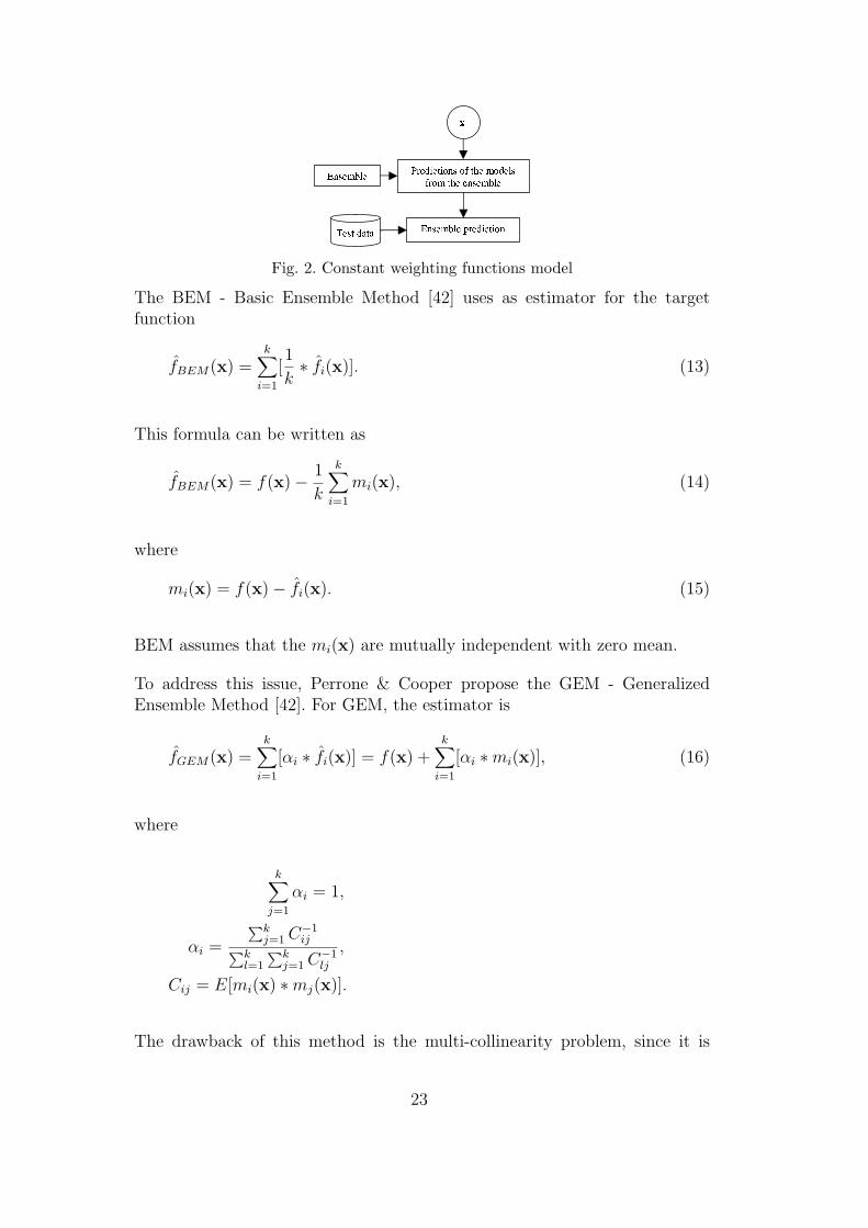
Fig. 2. Constant weighting functions model

The BEM - Basic Ensemble Method [42] uses as estimator for the targetfunction

fBEM(x) =k∑

i=1

[1

k∗ fi(x)]. (13)

This formula can be written as

fBEM(x) = f(x)− 1

k

k∑

i=1

mi(x), (14)

where

mi(x) = f(x)− fi(x). (15)

BEM assumes that the mi(x) are mutually independent with zero mean.

To address this issue, Perrone & Cooper propose the GEM - GeneralizedEnsemble Method [42]. For GEM, the estimator is

fGEM(x) =k∑

i=1

[αi ∗ fi(x)] = f(x) +k∑

i=1

[αi ∗mi(x)], (16)

where

k∑

j=1

αi = 1,

αi =

∑kj=1 C−1

ij∑kl=1

∑kj=1 C−1

lj

,

Cij = E[mi(x) ∗mj(x)].

The drawback of this method is the multi-collinearity problem, since it is

23

necessary to calculate the inverse matrix C−1. The multi-collinearity problemcan be avoided by pruning the ensemble [42] (Sect. 4).

The well known linear regression (LR) model is another possible combinationmethod. The predictor is the same as in GEM case but without the constraint∑k

j=1 αi = 1.

The use of a constant in the LR formula is not relevant in practice (the stan-dard linear regression formulation uses it) because E[fi(x)] ' E[f(x)] [67]. Itwould be necessary if predictors were meaningfully biased.

All the methods discussed so far suffer from the multi-collinearity problemwith the exception of BEM. Next we discuss methods that avoid this problem.

Caruana et al. embed the ensemble integration phase in the ensemble selectionone [22]. By selecting with replacement the models from the pool to include inthe ensemble, and using the simple average as the weighting function, the αi

coefficients are implicitly calculated as the number of times that each model isselected over the total number of models in the ensemble (including repeatedmodels).

Breiman presents the stacked regression [68] method based on the well knownstacked generalization framework [69] firstly presented for the classificationproblem. Given a L learning set with M examples, the goal is to obtain theαi coefficients that minimize

M∑

j=1

[f(xj)−k∑

i=1

αi ∗ fi(xj)]2. (17)

To do so, the learning set used to obtain the αi coefficients will be the same oneused to train the fi estimators, over-fitting the data. This problem is solvedby using υ-fold cross-validation,

M∑

j=1

[f(xj)−k∑

i=1

αi ∗ fi

(−υ)(xj)]

2. (18)

The second problem is the possible existence of multi-collinearity between thefi predictors. Breiman presents several approaches to obtain the αi coefficientsbut concludes that a method that gives consistently good results is the mini-mization of the above equation under the constraints αi ≥ 0, i = 1, ..., k [68].One of the methods tried by Breiman to obtain the αi coefficients is ridgeregression, a regression technique for solving badly conditioned problems. butresults were not promising [68]. An important result of Breiman is the empir-ical observation that, in most of the cases, many of the αi weights are zero.

24

This result supports the use of ensemble pruning as a second step after theensemble generation (Sect. 4).

Merz & Pazzani use principal component regression to avoid the multi-collinearityproblem [70]. The PCR* method obtains the principal components (PC) and,then, it selects the number of PCs to use. Once the PCs are ordered as afunction of the variation they can explain, the search of the number of PCs touse is much simplified. The choice of the correct number of PCs is importantto avoid under-fitting or over-fitting.

Evolutionary algorithms have also been used to obtain the αi coefficients [71].The used approach is globally better than BEM and GEM on twenty fiveclassification data sets. Compared to BEM wins nineteen, draws one and loosesfive. Compared to GEM wins seventeen, draws one and looses seven. Theseresults were obtained by direct comparison, i.e., without statistical validity.

The main study comparing constant weighting functions is presented by Merz[14]. The functions used are: GEM, BEM, LR, LRC (the LR formula with aconstant term), gradient descent, EG, EG+

− (the last three methods are gradi-ent descent procedures discussed by Kivinen & Warmuth [72]), ridge regres-sion, constrained regression (Merz [14] uses the bounded variable least squaresmethod from [73]), stacked constrained regression (with ten partitions) andPCR*. Two of the three experiments reported by Merz are summarized next.The first experiment used an ensemble of twelve models on eight regressiondata sets: six of the models were generated using MARS [74] and the othersix using the neural network back-propagation algorithm. The three globallybest functions were CR, EG and PCR*. The second experiment tests howthe functions perform with many correlated models. The author uses neuralnetwork ensembles of size ten and fifty. Just three data sets were used. ThePCR* function presents more robust results. See [14] to get details on theexperiments and their results.

5.2 Non-constant weighting functions

The non-constant weighting functions use different coefficients according tothe input for prediction. They can be static (defined at learning time) ordynamic (defined at prediction time). The static ones can use two differentapproaches: (1) to assign models to predefined regions, this is the divide-and-conquer approach already discussed in Sect. 3.1.1; or (2) to define theareas of expertise for each model, also called static selection [13], i. e., foreach predictor from the ensemble it is defined the input subspace where thepredictor is expert. In the dynamic approach the hi(x) weights from eq. 12are obtained on the fly based on the performances of the base predictors on

25

data similar to x obtained from the training set.

5.2.1 The approach by areas of expertise

The work on meta decision trees [75] for classification induces meta decisiontrees using as variables meta-attributes that are previously calculated for eachexample. The target variable of the meta tree is the classifier to recommend. Inpractice, the meta decision tree, instead of predicting, recommends a predictor.Despite this work has been developed for classification, it could be easilyadapted for regression by an appropriate choice of the meta attributes.

Yankov et al. use support vector machines with the gaussian kernel to selectthe predictor to use from an ensemble with two models [44].

5.2.2 The dynamic approach

In the dynamic approach, the predictor(s) selection is done on the fly, i.e.,given the input vector for the prediction task, it chooses the expected bestpredictor(s) to accomplish this task. While in the approach by areas of exper-tise these areas are previously defined, in the dynamic approach the areas aredefined on the fly. Selection can be seen as a kind of pruning on the fly. Themost usual way to select the predictor(s) is by evaluating their performanceson similar data from the training set, for a chosen performance metric. Oftenthe similar data is obtained by the use of the k-nearest neighbors with theEuclidean distance [76]. Puuronen et al. [77] use the more advanced weightedk-nearest neighbor.

Rooney et al. [10] adapt for regression the dynamic integration methods orig-inally presented by Puuronen et al. [77] for classification. Dynamic selection(DS) selects the predictor with less cumulative error on the k-nearest neighborsset. Dynamic weighting (DW) assigns a weight to each base model accordingto its localized performance on the k-nearest neighbors set [10] and the finalprediction is based on the weighted average of the predictions of the relatedmodels. Dynamic weighting with selection (DWS) is similar to DW but thepredictors with cumulative error in the upper half of the error interval arediscarded. From the three methods tested the DWS one using just the subsetof the most accurate predictors for the final prediction gets the best results.

Wang et al. use weights hi(x) (see eq. 12) inversely proportional to fi(x)expected error [78]. This approach is similar to the variance based weightingpresented in [79].

Figure 3 summarizes the dynamic approach. Given an input vector x, firstly itselects similar data. Then, according to the performance of the models on this

26

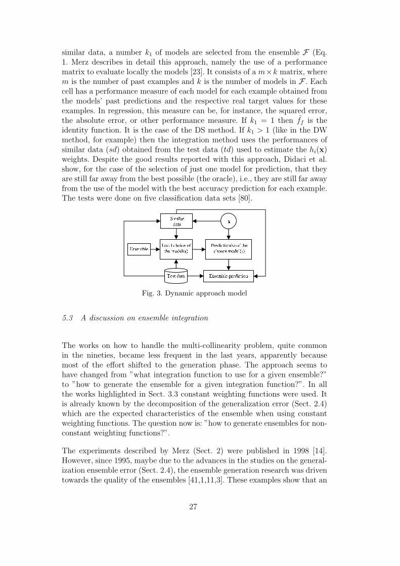
similar data, a number k1 of models are selected from the ensemble F (Eq.1. Merz describes in detail this approach, namely the use of a performancematrix to evaluate locally the models [23]. It consists of a m×k matrix, wherem is the number of past examples and k is the number of models in F . Eachcell has a performance measure of each model for each example obtained fromthe models’ past predictions and the respective real target values for theseexamples. In regression, this measure can be, for instance, the squared error,the absolute error, or other performance measure. If k1 = 1 then ff is theidentity function. It is the case of the DS method. If k1 > 1 (like in the DWmethod, for example) then the integration method uses the performances ofsimilar data (sd) obtained from the test data (td) used to estimate the hi(x)weights. Despite the good results reported with this approach, Didaci et al.show, for the case of the selection of just one model for prediction, that theyare still far away from the best possible (the oracle), i.e., they are still far awayfrom the use of the model with the best accuracy prediction for each example.The tests were done on five classification data sets [80].

Fig. 3. Dynamic approach model

5.3 A discussion on ensemble integration

The works on how to handle the multi-collinearity problem, quite commonin the nineties, became less frequent in the last years, apparently becausemost of the effort shifted to the generation phase. The approach seems tohave changed from ”what integration function to use for a given ensemble?”to ”how to generate the ensemble for a given integration function?”. In allthe works highlighted in Sect. 3.3 constant weighting functions were used. Itis already known by the decomposition of the generalization error (Sect. 2.4)which are the expected characteristics of the ensemble when using constantweighting functions. The question now is: ”how to generate ensembles for non-constant weighting functions?”.

The experiments described by Merz (Sect. 2) were published in 1998 [14].However, since 1995, maybe due to the advances in the studies on the general-ization ensemble error (Sect. 2.4), the ensemble generation research was driventowards the quality of the ensembles [41,1,11,3]. These examples show that an

27

important part of the problems at the integration phase can be solved by ajoint design of the generation, pruning (when appropriate) and the integrationphases.

The main disadvantage of constant weighting functions is that the αi weights,being equal for all the input space, can, at least theoretically, be less adequatefor some parts of the input space. This is the main argument for using non-constant weighting functions [81]. This argument can be particularly true fortime changing phenomena [78].

Ensemble integration approaches can also be classified as selection or combi-nation ones [13]. In the selection approach the final prediction is obtained byusing just one predictor, while in the combination one the final prediction isobtained by combining predictions of two or more models. Kuncheva presentsan hybrid approach between the selection and the combination ones [13]. Ituses paired t-hypothesis test to verify if there is one predictor meaningfullybetter than the others. If positive, it uses the best predictor, if not it uses acombination approach.

An approach that can be explored and seems to be promising is to combinedifferent ensemble integration methods. The method wMetaComb [82] uses aweighted average to combine stacked regression (described in Sect. 5.1) andthe DWS dynamic method (Sect. 5.2.2). The weights are determined basedon the error performance of both methods (see [82] for details). Tests on 30regression data sets never looses against stacked regression (it wins 5 anddraws the remaining 25) and looses 3 against DWS (it wins 13 and draws 14).

6 Conclusions

The use of ensemble methods has as main advantages the increase in accuracyand robustness, when compared to the use of a single model. This makes en-semble methods particularly suited for applications where small improvementsof the predictions have important impact.

For ensemble learning, as for other research areas, methods for regressionand for classification have different solutions, at least partially. This paper isfocused in the regression problem, less referred in the literature. The methodsfor ensemble learning have, typically, three phases: generation, pruning (notalways) and integration.

The generation phase aims to obtain an ensemble of models. It can be classi-fied as homogeneous or as heterogeneous. This classification depends on theinduction algorithms used. If just one is used, the ensemble is classified as

28

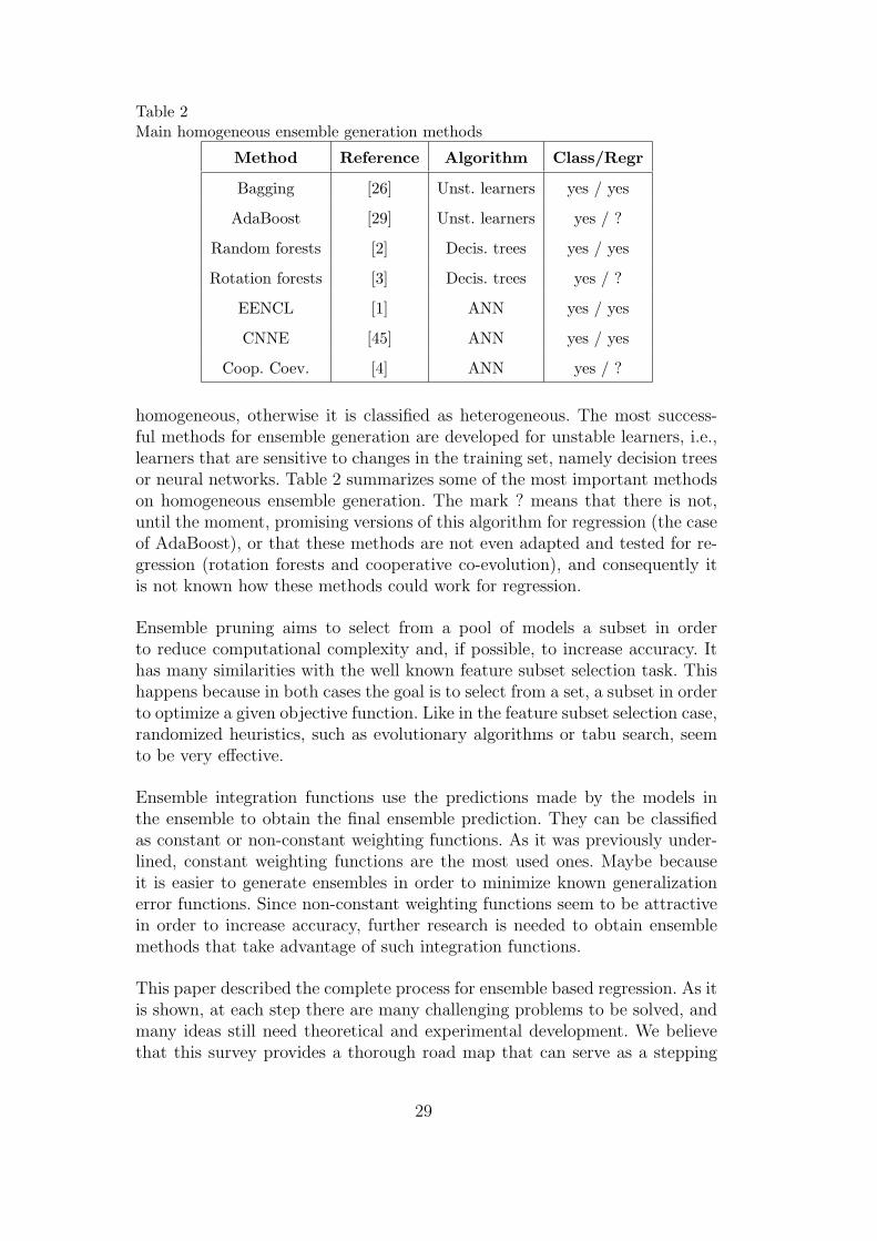
Table 2Main homogeneous ensemble generation methods

Method Reference Algorithm Class/Regr

Bagging [26] Unst. learners yes / yes

AdaBoost [29] Unst. learners yes / ?

Random forests [2] Decis. trees yes / yes

Rotation forests [3] Decis. trees yes / ?

EENCL [1] ANN yes / yes

CNNE [45] ANN yes / yes

Coop. Coev. [4] ANN yes / ?

homogeneous, otherwise it is classified as heterogeneous. The most success-ful methods for ensemble generation are developed for unstable learners, i.e.,learners that are sensitive to changes in the training set, namely decision treesor neural networks. Table 2 summarizes some of the most important methodson homogeneous ensemble generation. The mark ? means that there is not,until the moment, promising versions of this algorithm for regression (the caseof AdaBoost), or that these methods are not even adapted and tested for re-gression (rotation forests and cooperative co-evolution), and consequently itis not known how these methods could work for regression.

Ensemble pruning aims to select from a pool of models a subset in orderto reduce computational complexity and, if possible, to increase accuracy. Ithas many similarities with the well known feature subset selection task. Thishappens because in both cases the goal is to select from a set, a subset in orderto optimize a given objective function. Like in the feature subset selection case,randomized heuristics, such as evolutionary algorithms or tabu search, seemto be very effective.

Ensemble integration functions use the predictions made by the models inthe ensemble to obtain the final ensemble prediction. They can be classifiedas constant or non-constant weighting functions. As it was previously under-lined, constant weighting functions are the most used ones. Maybe becauseit is easier to generate ensembles in order to minimize known generalizationerror functions. Since non-constant weighting functions seem to be attractivein order to increase accuracy, further research is needed to obtain ensemblemethods that take advantage of such integration functions.

This paper described the complete process for ensemble based regression. As itis shown, at each step there are many challenging problems to be solved, andmany ideas still need theoretical and experimental development. We believethat this survey provides a thorough road map that can serve as a stepping

29

stone to new ideas for research.

Acknowledgements

This work was partially supported by FCT (POCT/TRA/61001/2004) andFEDER e Programa de Financiamento Plurianual de Unidades de I&D.

References

[1] Yong Liu, Xin Yao, and Tetsuya Higuchi, “Evolutionary ensembleswith negative correlation learning”, IEEE Transactions on EvolutionaryComputation, vol. 4, no. 4, pp. 380–387, 2000.

[2] Leo Breiman, “Random forests”, Machine Learning, vol. 45, pp. 5–32, 2001.

[3] Juan J. Rodrıguez, Ludmila I. Kuncheva, and Carlos J. Alonso, “Rotationforest: a new classifier ensemble”, IEEE Transactions on Pattern Analysis andMachine Intelligence, vol. 28, no. 10, pp. 1619–1630, 2006.

[4] Nicolas Garcıa-Pedrajas, Cesar Hervas-Martınez, and Domingo Ortiz-Boyer,“Cooperative coevolution of artificial neural network ensembles for patternclassification”, IEEE Transactions on Evolutionary Computation, vol. 9, no.3, pp. 271–302, 2005.

[5] Ludmila I. Kuncheva, Combining pattern classifiers, Wiley, 2004.

[6] Romesh Ranawana and Vasile Palade, “Multi-classifier systems: review and aroadmap for developers”, International Journal of Hybrid Intelligent Systems,vol. 3, no. 1, pp. 35–61, 2006.

[7] Thomas G. Dietterich, “Machine-learning research: four current directions”, AImagazine, vol. 18, no. 4, pp. 97–136, 1997.

[8] Alexander Strehl and Joydeep Ghosh, “Cluster ensembles - a knowledge reuseframework for combining multiple partitions”, Journal of Machine LearningResearch, vol. 3, pp. 583–617, 2003.

[9] Fabio Roli, Giorgio Giacinto, and Gianni Vernazza, “Methods for designingmultiple classifier systems”, in International Workshop on Multiple ClassifierSystems. 2001, vol. LNCS 2096, pp. 78–87, Springer.

[10] Niall Rooney, David Patterson, Sarab Anand, and Alexey Tsymbal, “Dynamicintegration of regression models”, in International Workshop on MultipleClassifier Systems. 2004, vol. LNCS 3181, pp. 164–173, Springer.

[11] Zhi-Hua Zhou, Jianxin Wu, and Wei Tang, “Ensembling neural networks: manycould be better than all”, Artificial Intelligence, vol. 137, pp. 239–263, 2002.

30

[12] Gonzalo Martınez-Munoz and Alberto Suarez, “Pruning in ordered baggingensembles”, in International Conference on Machine Learning, 2006, pp. 609–616.

[13] Ludmila I. Kuncheva, “Switching between selection and fusion in combiningclassifiers: an experiment”, IEEE Transactions on Systems, Man, andCybernetics-Part B, vol. 32, no. 2, pp. 146–156, 2002.

[14] Cristopher J. Merz, Classification and regression by combining models, Phdthesis, University of California - U.S.A., 1998.

[15] Trevor Hastie, Robert Tibshirani, and Jerome H. Friedman, The elements ofstatistical learning: data mining, inference, and prediction, Springer series instatistics. Springer, 2001.

[16] Gavin Brown, Diversity in neural network ensembles, Phd thesis, University ofBirmingham - United Kingdom, 2004.

[17] Stuart Geman, Elie Bienenstock, and Rene Doursat, “Neural networks and thebias/variance dilemma”, Neural Computation, vol. 4, no. 1, pp. 1–58, 1992.

[18] Anders Krogh and Jesper Vedelsby, “Neural network ensembles, crossvalidation, and active learning”, Advances in Neural Information ProcessingSystems, vol. 7, pp. 231–238, 1995.

[19] Naonori Ueda and Ryohei Nakano, “Generalization error of ensembleestimators”, in IEEE International Conference on Neural Networks, 1996,vol. 1, pp. 90–95.

[20] Gavin Brown, Jeremy L. Wyatt, Rachel Harris, and Xin Yao, “Diversitycreation methods: a survey and categorisation”, Information Fusion, vol. 6,pp. 5–20, 2005.

[21] Geoffrey I. Webb and Zijian Zheng, “Multistrategy ensemble learning: reducingerror by combining ensemble learning techniques”, IEEE Transactions onKnowledge and Data Engineering, vol. 16, no. 8, pp. 980–991, 2004.

[22] Rich Caruana, Alexandru Niculescu-Mozil, Geoff Crew, and Alex Ksikes,“Ensemble selection from libraries of models”, in International Conference onMachine Learning, 2004.

[23] Cristopher J. Merz, “Dynamical selection of learning algorithms”, inInternational Workshop on Artificial Intelligence and Statistics, D. Fisher andH.-J. Lenz, Eds. 1996, vol. Learning from Data: Artificial Intelligence andStatistics V, Springer-Verlag.

[24] Leo Breiman, “Heuristics of instability and stabilization in model selection”,Annals of Statistics, vol. 24, no. 6, pp. 2350–2383, 1996.

[25] Hyun-Chul Kim, Shaoning Pang, Hong-Mo Je, Daijin Kim, and Sung-YangBang, “Constructing support vector machine ensemble”, Pattern Recognition,vol. 36, no. 12, pp. 2757–2767, 2003.

31

[26] Leo Breiman, “Bagging predictors”, Machine Learning, vol. 26, pp. 123–140,1996.

[27] Pedro Domingos, “Why does bagging work? a bayesian account and itsimplications”, in International Conference on Knowledge Discovery and DataMining. 1997, pp. 155–158, AAAI Press.

[28] R. Schapire, “The strength of weak learnability”, Machine learning, vol. 5, no.2, pp. 197–227, 1990.

[29] Y. Freund and R. Schapire, “Experiments with a new boosting algorithm”, inInternational Conference on Machine Learning, 1996, pp. 148–156.

[30] P.M. Granitto, P.F. Verdes, and H.A. Ceccatto, “Neural network ensembles:evaluation of aggregation algorithms”, Artificial Intelligence, vol. 163, no. 2,pp. 139–162, 2005.

[31] Bambang Parmanto, Paul W. Munro, and Howard R. Doyle, “Reducingvariance of committee prediction with resampling techniques”, ConnectionScience, vol. 8, no. 3, 4, pp. 405–425, 1996.

[32] Tin Kam Ho, “The random subspace method for constructing decision forests”,IEEE Transactions on Pattern Analysis and Machine Intelligence, vol. 20, no.8, pp. 832–844, 1998.

[33] David W. Opitz, “Feature selection for ensembles”, in 16th National Conferenceon Artificial Intelligence, Orlando - U.S.A., 1999, pp. 379–384, AAAI Press.

[34] Gabriele Zenobi and Padraig Cunningham, “Using diversity in preparingensembles of classifiers based on different feature subsets to minimizegeneralization error”, in European Conference on Machine Learning. 2001, vol.LNCS 2167, pp. 576–587, Springer.

[35] Carlotta Domeniconi and Bojun Yan, “Nearest neighbor ensemble”, inInternational Conference on Pattern Recognition, 2004, vol. 1, pp. 228–231.

[36] Eibe Frank and Bernhard Pfahringer, “Improving on bagging with inputsmearing”, in Pacific-Asia Conference on Knowledge Discovery and DataMining. 2006, pp. 97–106, Springer.

[37] Yuval Raviv and Nathan Intrator, “Bootstrapping with noise: an effectiveregularization technique”, Connection Science, vol. 8, no. 3, 4, pp. 355–372,1996.

[38] Leo Breiman, “Randomizing outputs to increase prediction accuracy”, MachineLearning, vol. 40, no. 3, pp. 229–242, 2000.

[39] Leo Breiman, “Using iterated bagging to debias regressions”, Machine Learning,vol. 45, no. 3, pp. 261–277, 2001.

[40] John F. Kolen and Jordan B. Pollack, “Back propagation is sensitive to initialconditions”, Tech. Report TR 90-JK-BPSIC, The Ohio State University, 1990.

32

[41] Bruce E. Rosen, “Ensemble learning using decorrelated neural networks”,Connection Science, vol. 8, no. 3, 4, pp. 373–383, 1996.

[42] Michael P. Perrone and Leon N. Cooper, “When networks disagree: ensemblemethods for hybrid neural networks”, in Neural Networks for Speech and ImageProcessing, R.J. Mammone, Ed. Chapman-Hall, 1993.

[43] Sherif Hashem, Optimal linear combinations of neural networks, Phd thesis,Purdue University, 1993.

[44] Dragomir Yankov, Dennis DeCoste, and Eamonn Keogh, “Ensembles of nearestneighbor forecasts”, in European Conference on Machine Learning. 2006, vol.LNAI 4212, pp. 545–556, Springer.

[45] Md. Monirul Islam, Xin Yao, and Kazuyuki Murase, “A constructive algorithmfor training cooperative neural network ensembles”, IEEE Transactions onNeural Networks, vol. 14, no. 4, pp. 820–834, 2003.

[46] Ivor W. Tsang, Andras Kocsor, and James T. Kwok, “Diversified svm ensemblesfor large data sets”, in European Conference on Machine Learning. 2006, vol.LNAI 4212, pp. 792–800, Springer.

[47] Ivor W. Tsang, James T. Kwok, and Kimo T. Lai, “Core vector regressionfor very large regression problems”, in International Conference on MachineLearning, 2005, pp. 912–919.

[48] Y. Liu and X. Yao, “Ensemble learning via negative correlation”, NeuralNetworks, vol. 12, pp. 1399–1404, 1999.

[49] David W. Opitz and Jude W. Shavlik, “Generating accurate and diversemembers of a neural-network ensemble”, Advances in Neural InformationProcessing Systems, vol. 8, pp. 535–541, 1996.

[50] Hsuan-Tien Lin and Ling Li, “Infinite ensemble learning with support vectormachines”, in European Conference on Machine Learning. 2005, vol. LNAI3720, pp. 242–254, Springer.

[51] Alıpio M. Jorge and Paulo J. Azevedo, “An experiment with associationrules and classification: post-bagging and conviction”, in Discovery science,Singapore, 2005, vol. LNCS 3735, pp. 137–149, Springer.

[52] Paulo J. Azevedo and Alıpio Mario Jorge, “Iterative reordering of rules forbuilding ensembles without relearning”, in 10th International Conference onDicovery Science. 2007, vol. LNCS 4755, pp. 56–67, Springer.

[53] David Meyer, Friedrich Leisch, and Kurt Hornik, “The support vector machineunder test”, Neurocomputing, vol. 55, no. 1-2, pp. 169–186, 2003.

[54] Bart Bakker and Tom Heskes, “Clustering ensembles of neural network models”,Neural Networks, vol. 16, no. 2, pp. 261–269, 2003.

[55] Christino Tamon and Jie Xiang, “On the boosting pruning problem”, inEuropean Conference on Machine Learning. 2000, vol. LNCS 1810, pp. 404–412, Springer.

33

[56] Matti Aksela, “Comparison of classifier selection methods for improvingcommittee performance”, in International Workshop on Multiple ClassifierSystems. 2003, vol. LNCS 2709, pp. 84–93, Springer.

[57] D. Partridge and W. B. Yates, “Engineering multiversion neural-ney systems”,Neural Computation, vol. 8, no. 4, pp. 869–893, 1996.

[58] Zhi-Hua Zhou and Wei Tang, “Selective ensemble of decision trees”, inInternational Conference on Rough Sets, Fuzzy Sets, Data Mining, andGranular Computing. 2003, vol. LNAI 2639, pp. 476–483, Springer.

[59] Dymitr Ruta and Bogdan Gabrys, “Application of the evolutionary algorithmsfor classifier selection in multiple classifier systems with majority voting”, inInternational Workshop on Multiple Classifier Systems. 2001, vol. LNCS 2096,pp. 399–408, Springer.

[60] Guilherme P. Coelho and Fernando J. Von Zuben, “The influence of the poolof candidates on the performance of selection and combination techniques inensembles”, in International Joint Conference on Neural Networks, 2006, pp.10588–10595.

[61] Daniel Hernandez-Lobato, Gonzalo Martınez-Munoz, and Alberto Suarez,“Pruning in ordered regression bagging ensembles”.

[62] Joao M. Moreira, Jorge Freire Sousa, Alıpio M. Jorge, and Carlos Soares, “Anensemble regression approach for bus trip time prediction”, in Meeting of theEURO Working Group on Transportation, 2006, pp. 317–321.

[63] Dragos D. Margineantu and Thomas G. Dietterich, “Pruning adaptiveboosting”, in International Conference on Machine Learning, 1997, pp. 211–218.

[64] S.B. Kotsiantis and P.E. Pintelas, “Selective averaging of regression models”,Annals of Mathematics, Computing & Teleinformatics, vol. 1, no. 3, pp. 65–74,2005.

[65] Aleksandar Lazarevic, “Effective pruning of neural network classifierensembles”, in International Joint Conference on Neural Networks, 2001, pp.796–801.

[66] Giorgio Giacinto and Fabio Roli, “Design of effective neural network ensemblesfor image classification purposes”, Image and Vision Computing, vol. 19, no. 9,pp. 699–707, 2001.

[67] Michael LeBlanc and Robert Tibshirani, “Combining estimates in regressionand classification”, Journal of the American Statistical Association, vol. 91, pp.1641–1650, 1996.

[68] Leo Breiman, “Stacked regressions”, Machine Learning, vol. 24, pp. 49–64,1996.

[69] David H. Wolpert, “Stacked generalization”, Neural Networks, vol. 5, no. 2,pp. 241–259, 1992.

34

[70] Cristopher J. Merz and Michael J. Pazzani, “A principal components approachto combining regression estimates”, Machine Learning, vol. 36, pp. 9–32, 1999.

[71] Domingo Ortiz-Boyer, Cesar Hervas-Martınez, and Nicolas Garcıa-Pedrajas,“Cixl2: A crossover operator for evolutionary algorithms based on populationfeatures”, Journal of Artificial Intelligence Research, vol. 24, pp. 1–48, 2005.

[72] Jyrki Kivinen and Manfred K. Warmuth, “Exponentiated gradient versusgradient descent for linear predictors”, Information and Computation, vol. 132,no. 1, pp. 1–63, 1997.

[73] P. Stark and R. Parker, “Bounded-variable least squares: an algorithm andapplications”, Computational Statistics, vol. 10, no. 2, pp. 129–141, 1995.

[74] J.H. Friedman, “Multivariate adaptive regression splines”, The Annals ofStatistics, vol. 19, no. 1, pp. 1–141, 1991.

[75] Ljupco Todorovski and Saso Dzeroski, “Combining classifiers with metadecision trees”, Machine Learning, vol. 50, no. 3, pp. 223–249, 2003.

[76] Kevin Woods, “Combination of multiple classifiers using local accuracyestimates”, IEEE Transactions on Pattern Analysis and Machine Intelligence,vol. 19, no. 4, pp. 405–410, 1997.

[77] Seppo Puuronen, Vagan Terziyan, and Alexey Tsymbal, “A dynamic integrationalgorithm for an ensemble of classifiers”, in International Symposium onMethodologies for Intelligent Systems. 1999, vol. LNCS 1609, pp. 592–600,Springer.

[78] Haixun Wang, Wei Fan, Philip S. Yu, and Jiawei Han, “Mining concept-driftingdata streams using ensemble classifiers”, in ACM International Conference onKnowledge Discovery and Data Mining, 2003.

[79] Volker Tresp and Michiaki Taniguchi, “Combining estimators using non-constant weighting functions”, Advances in Neural Information ProcessingSystems, vol. 7, pp. 419–426, 1995.

[80] Luca Didaci, Giorgio Giacinto, Fabio Roli, and Gian Luca Marcialis, “A studyon the performances of dynamic classifier selection based on local accuracyestimation”, Pattern Recognition, vol. 38, no. 11, pp. 2188–2191, 2005.

[81] Antanas Verikas, Arunas Lipnickas, Kerstin Malmqvist, Marija Becauskiene,and Adas Gelzinis, “Soft combining of neural classifiers: a comparative study”,Pattern Recognition Letters, vol. 20, no. 4, pp. 429–444, 1999.

[82] Niall Rooney and David Patterson, “A weighted combination of stacking anddynamic integration”, Pattern Recognition, vol. 40, no. 4, pp. 1385–1388, 2007.

35