Origin of the initial mass function

Lecture 7 supplementary slidesDaniel Price

Initial Mass Function

masses of 0.3–0.6M!. In summary, according to the best avail-able data, the brown dwarf fractions in Taurus and IC 348 arelower than in the Trapezium, but by a smaller factor (1.4–1.8)than that reported in earlier studies.

5.1.2. Stars

In logarithmic units where the Salpeter slope is 1.35, theIMFs for IC 348 and the Trapezium cluster rise from highmasses down to a solar mass, rise more slowly down to amaximum at 0.1–0.2 M!, and then decline into the substellarregime (Luhman et al. 2003b; Muench et al. 2002, 2003;Slesnick et al. 2004). In comparison, the IMF for Taurus risesquickly to a peak near 0.8 M! and steadily declines to lowermasses (Briceno et al. 2002; Luhman et al. 2003a; Fig. 13).The distinctive shapes of the IMFs in IC 348 and Taurus arereflected in the distributions of spectral types, which shouldcomprise good observational proxies of the IMFs (Luhmanet al. 2003b; Fig. 12). These significant differences betweenTaurus and the other two clusters remain, regardless of the de-gree of incompleteness in the Taurus IMF at 0.3–0.6 M!.

At stellar masses, Kroupa et al. (2003) found that the IMFfor unresolved systems from their standard model was nearlyidentical to the IMF for Taurus from Luhman et al. (2003a) andthe IMF for Orion from Muench et al. (2002). As a result, theyconcluded that these IMFs for Taurus and Orion ‘‘can beconsidered very similar if not identical’’ and ‘‘only in the sub-stellar mass regime may the observations indicate different

mass functions.’’ However, this is clearly not the case. As de-scribed above, the IMF for Taurus differs significantly from thatof IC 348, which in turn closely matches the IMF for the Tra-pezium at stellar masses (Muench et al. 2002, 2003; Slesnicket al. 2004). This difference between Taurus and IC 348 hasbeen shown to be highly statistically significant (Luhman et al.2003b). As an additional illustration of the obvious differencesin the IMFs between Taurus and the two other clusters, theTrapezium IMF from Muench et al. (2002) is shown with themass functions of Taurus and IC 348 in Figure 13. The distinctnature of the IMF in Taurus is also evident in the distribution ofspectral types in Figure 12, as pointed out by Luhman et al.(2003b).

5.2. Model Predictions for the IMF

A simple theoretical explanation for the above variations inthe IMF was offered along with the data by Briceno et al.(2002) and Luhman et al. (2003b). These authors suggestedthat the lower brown dwarf fraction and higher peak mass inTaurus relative to the Trapezium could reflect differences in thetypical Jeans masses of the two regions. Other possible sourcesfor these variations are investigated in this section.

5.2.1. Ejection

Kroupa & Bouvier (2003b) simulated the brown dwarffractions in the Trapezium and Taurus under the assumptionthat the brown dwarfs form through ejection with the same one-dimensional velocity dispersion, !ej, in each region. This modelpredicted that ejected brown dwarfs remain in the Trapeziumfor !ej < 6 km s"1 and escape a D # 1$ field in Taurus for!ej > 1:5 km s"1. At !ej % 2 km s"1, the simulated brown dwarffractions in the Trapezium and in 1$ Taurus fields agreed withthe measurements available at that time. As a result, Kroupa &Bouvier (2003b) suggested that the lower brown dwarf fractionin the Taurus aggregates relative to the Trapezium may be dueto the formation of brown dwarfs via ejection and that a dis-tributed population of predominantly single brown dwarfs mayexist outside of the fields surveyed in Taurus. To account for a‘‘disconcerting discrepancy’’ between the brown dwarf frac-tions in star-forming regions (%0.25) and the galactic field(%1), Kroupa & Bouvier (2003b) also examined a variationof this model in which the ejection process is not identical inall regions. In this scenario, brown dwarfs and stars form inroughly equal numbers in Taurus, but most of the brown dwarfsescape to sufficient distances that they are missed by currentsurveys. Meanwhile, brown dwarfs are produced at a quarter ofthe rate of stars in the Trapezium, most of which are retained inthe cluster and thus counted in observations. This model wouldindicate that the brown dwarfs in the field are predominantlyformed in low-density regions like Taurus. In search of furthersupport for the ejection model for brown dwarf formation,Kroupa & Bouvier (2003b) and Kroupa et al. (2003) contendedthat brown dwarfs do not share the same general formationhistory of stars because their binary properties are not a naturalextension of those of low-mass stars.

Two aspects of these hypotheses from Kroupa & Bouvier(2003b) and Kroupa et al. (2003) warrant discussion. First,Kroupa & Bouvier (2003b) referred to a deficiency of browndwarfs in star-forming regions relative to the field, but thisdeficiency is not supported by the available data. They quotedbrown dwarf fractions of 0.25 and 1 for star-forming regionsand the field, referencing the various studies of the Trapeziumand the analysis of field data by Chabrier (2002). However, acomparison of substellar mass functions of young clusters and

Fig. 13.—IMFs for extinction-limited samples (AV & 4) in fields 1 and 2 inTaurus (this work, top) and in a 160 ; 140 field in IC 348 (Luhman et al. 2003b,middle). These samples are unbiased in mass for M=M! ' 0:02 and 0.03,respectively, except for possible incompleteness at M=M! # 0:3 0:6 inTaurus (x 3.4). For comparison, an IMF derived from luminosity functionmodeling of the Trapezium cluster in Orion is also shown (Muench et al.2002, bottom). In the units of this diagram, the Salpeter slope is 1.35.

BROWN DWARFS AND IMF IN TAURUS 1229No. 2, 2004 Luhman (2004)

Carpenter, 2000), in the Pleiades (Hambly et al., 1999),and in the cluster M35 (Barrado y Navascues et al.,2001).

The most popular approach to approximating the IMFempirically is to use a multiple-component power law ofthe form of Eq. (8) with the following parameters(Scalo, 1998; Kroupa, 2002):

!"m #!! 0.26 m"0.3 for 0.01$m#0.08

0.035 m"1.3 for 0.08$m#0.5

0.019 m"2.3 for 0.5$m#% .(11)

This representation of the IMF is statistically cor-rected for binary and multiple stellar systems too closeto be resolved, but too far apart to be detected spectro-scopically. Neglecting these systems overestimates themasses of stars, as well as reducing inferred stellar den-sities. These mass overestimates influence the derivedstellar mass distribution, underestimating the number oflow-mass stars. The IMF may steepen further towardshigh stellar masses and a fourth component could be

defined with !(m)!0.019m"2.7 for m$1.0, thus arrivingat the IMF proposed by Kroupa, Tout, and Gilmore(1993). In Eq. (11), the exponents for masses m#0.5 arevery uncertain due to the difficulty of detecting and de-termining the masses of very young low-mass stars. Theexponent for 0.08$m#0.5 could vary between "0.7 and"1.8, and the value in the substellar regime is even lesscertain.

There are some indications that the slope of the massspectrum obtained from field stars may be slightly shal-lower than the one obtained from observing stellar clus-ters (Scalo, 1998). The reason for this difference is un-known. It is somehow surprising, given the fact mostfield stars appear to come from dissolved clusters (Ad-ams and Myers, 2001). It is possible that the field starIMF is inaccurate because of incorrect assumptionsabout past star formation rates and age dependences forthe stellar scale height. Both issues are either known orirrelevant for the IMF derived from cluster surveys. Onthe other hand, the cluster surveys could have failed toinclude low-mass stars due to extinction or crowding. Ithas also been claimed that the IMF may vary betweendifferent stellar clusters (Scalo, 1998), as the measuredexponent & in each mass interval exhibits considerablescatter when comparing different star-forming regions.This is illustrated in Fig. 6, which is again taken fromKroupa (2002). This scatter, however, may be entirelydue to effects related to the dynamical evolution of stel-lar clusters (Kroupa, 2001).

Despite these differences in detail, all IMF determina-tions share the same basic features, and it appears rea-sonable to say that the basic shape of the IMF is a uni-versal property common to all star-forming regions inthe present-day Galaxy, perhaps with some intrinsicscatter. There still may be some dependency on the me-tallicity of the star-forming gas, but changes in the IMFdo not seem to be gross even in that case. There is nocompelling evidence for qualitatively different behaviorsuch as truncation at the low- or high-mass end.

III. HISTORICAL DEVELOPMENT

Stars form from gravitational contraction of gas anddust in molecular clouds. A first estimate of the stabilityof such a system against gravitational collapse can bemade by simply considering its energy balance. For in-stability to occur, gravitational attraction must overcomethe combined action of all dispersive or resistive forces.In the simplest case, the absolute value of the potentialenergy of a system in virial equilibrium is exactly twicethe total kinetic energy, Epot%2 Ekin!0. If Epot%2 Ekin#0 the system collapses, while for Epot%2 Ekin$0 it ex-pands. This estimate can easily be extended by includingthe surface terms and additional physical forces (see fur-ther discussion in Sec. II.D). In particular, taking mag-netic fields into account may become important for de-scribing interstellar clouds (Chandrasekhar and Fermi,1953b; see also McKee et al., 1993, for a more recentdiscussion). In the presence of turbulence, the total ki-

FIG. 5. (Color in online edition) The measured stellar massfunction ! as a function of logarithmic mass log10 m in theOrion nebular cluster (upper circles), the Pleiades (trianglesconnected by line), and the cluster M35 (lower circles). Noneof the mass functions is corrected for unresolved multiple stel-lar systems. The average initial stellar mass function derivedfrom Galactic field stars in the solar neighborhood is shown asa line with the associated uncertainty range indicated by thehatched area. From Kroupa, 2002.

137M.-M. Mac Low and R. S. Klessen: Control of star formation by supersonic turbulence

Rev. Mod. Phys., Vol. 76, No. 1, January 2004

Kroupa (2002)

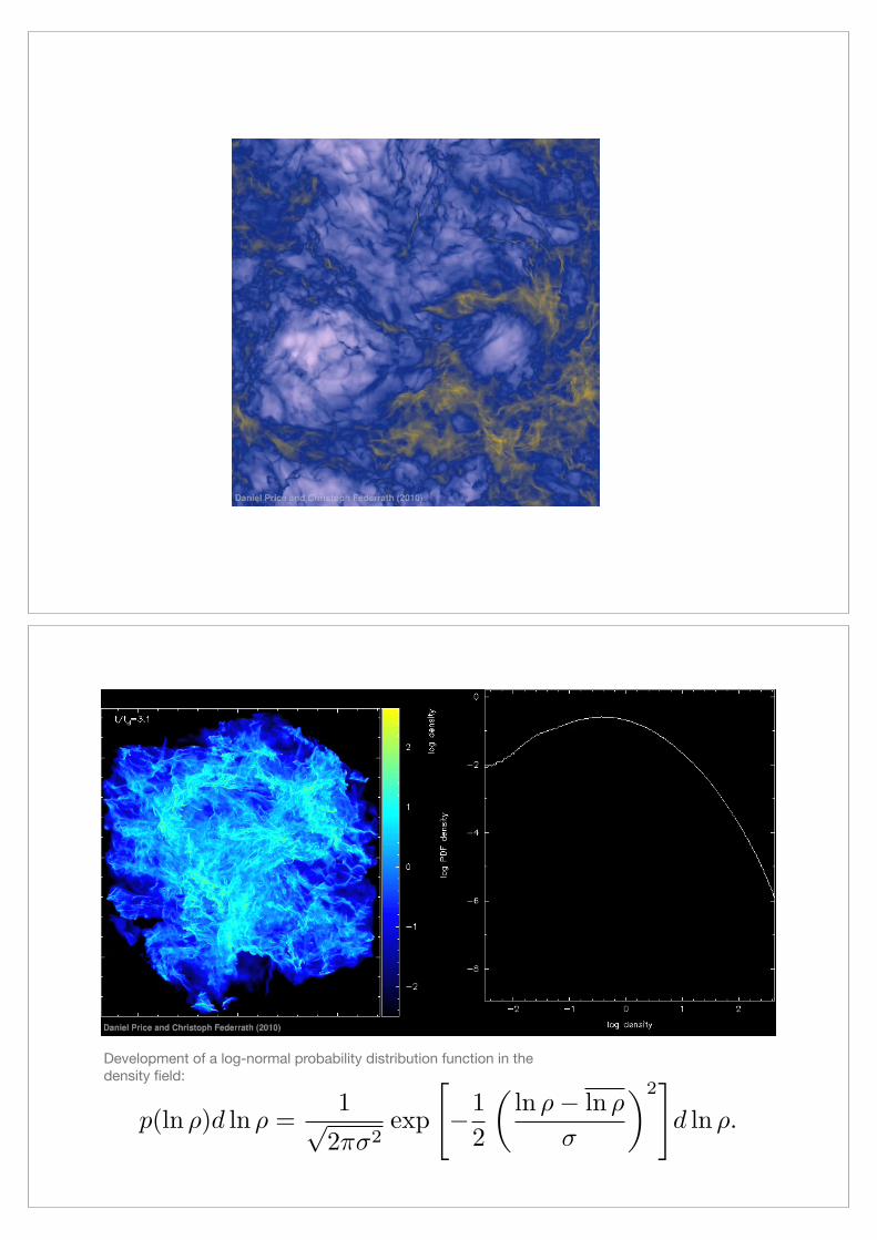
Development of a log-normal probability distribution function in the density field:

p(ln ρ)d ln ρ =1√

2πσ2exp

�−1

2

�ln ρ− ln ρ

σ

�2�d ln ρ.

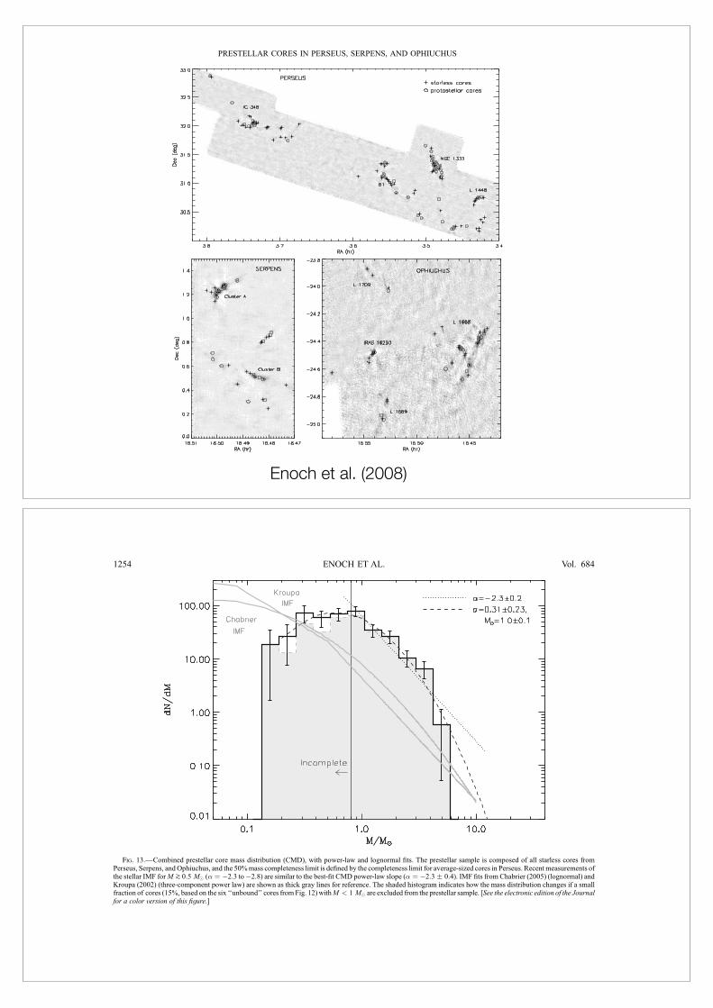
level, and positions are determined using a surface-brightness-weighted centroid, as described in Paper III. The Bolocam mapsof Perseus, Serpens, and Ophiuchus are shown in Figure 3, withthe positions of starless and protostellar cores indicated. Theaverage 1 ! rms is 15 mJy beam!1 in Perseus, 10 mJy beam!1 inSerpens, and 25 mJy beam!1 in Ophiuchus.

General core statistics, including the number of starless (NSL)and protostellar (NPS) cores in each cloud, as well as the ratioNSL /NPS , are given in Table 3. Note that the number of starlessand protostellar cores are approximately equal in each cloud(NSL /NPS " 1:2 in Perseus, 0.8 in Serpens, and 1.4 inOphiuchus),a fact that will be important for our discussion of the starless corelifetime in x 6. The last column of Table 3 gives the number ofindividual 1.1 mm cores that are associated with more than one

Fig. 3.—Bolocam maps of Perseus, Serpens, and Ophiuchus, with the positions of starless and protostellar cores indicated. Identified cores have peak flux densities of atleast 5 !, where ! is the local rms noise level (on average! " 15 mJy beam!1 in Perseus, 10mJy beam!1 in Serpens, and 25 mJy beam!1 in Ophiuchus). Note that due to thelarge scales, individual structures are difficult to see. Regions of the maps with no detected sources have been trimmed for this figure. Starless and protostellar cores clustertogether throughout each cloud, with both populations tending to congregate along filamentary cloud structures. There are a few exceptional regions, however, which aredominated by either starless or protostellar cores (e.g., the B1 ridge, Serpens cluster A). [See the electronic edition of the Journal for a color version of this figure.]

TABLE 3

Statistics of 1.1 mm Cores in the Three Clouds

Cloud Ntotala NSL

b NPSc NSL /NPS NPS (Multiple)d

Perseus ................ 122 67 55 1.2 13

Serpens ................ 35 15 20 0.8 11Ophiuchus ........... 43 26 17 1.5 3

a Total number of identified 1.1 mm cores.b Number of starless 1.1 mm cores, i.e., cores that do not have a protostar

candidate located within 1:0 ; "1 mm of the core position.c Number of protostellar cores.d Number of protostellar cores that are associated with more than one can-

didate cold protostar (each within 1:0 ; "1 mm of the core position).

PRESTELLAR CORES IN PERSEUS, SERPENS, AND OPHIUCHUS 1245

Enoch et al. (2008)

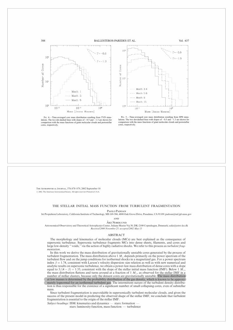
also taking into account formal fitting errors. We fit a lognormaldistribution toM > 0:3 M!, finding a best-fit width ! " 0:30#0:03 and characteristic massM0 " 1:0 # 0:1 M!. Although thelognormal function is quite a good fit ("2 " 0:5), the reliabilityof the turnover in the prestellar CMD is highly questionablegiven that the completeness limit in Perseus coincides closelywith the turnover mass. The prestellar CMD can also be fit by abroken power law with # " $4:3 # 1:1 for M > 2:5 M! and# " $1:7 # 0:3 for M < 2:5 M!, although the uncertaintiesare large.

Given that source detection is based on peak intensity, wemaybe incomplete to sources with very large sizes and low surfacedensity even in the higher mass bins (M > 0:8 M!). Complete-ness varies with size similarly to M / R2; thus the fraction of(possibly) missed sources should decrease with increasingmass.11

The effect of missing such low-surface-brightness cores, if theyexist and could be considered prestellar, would be to flatten theCMD slightly (i.e., the true slope would be steeper than the ob-served slope). Instrumental selection effects are discussed furtherin Paper I.

To be completely consistent, we should exclude the ‘‘unbound’’cores from Figure 12 (those with Mdust /Mvir < 0:5) from ourprestellar CMD. This represents 6 out of the 40 cores that havemeasured virial masses in Perseus, all 6 of which have Mdust <1 M!. We do not have virial masses for cores in Serpens orOphiuchus, but we can randomly remove a similar fraction ofsources withM < 1 M! from each cloud sample (2 sources from

Serpens, 4 from Ophiuchus, and an additional 4 from Perseus).The shaded histogram in Figure 13 indicates how the mass dis-tribution is altered when these 16 ‘‘unbound’’ cores are excludedfrom the sample. Our derived CMD slope is not affected, as nearlyall of the starless cores below the ‘‘gravitationally bound’’ line inFigure 12 have masses below our completeness limit, and evenat low masses the CMD is not significantly changed.There may also be some concern over the use of a single dust

temperature TD " 10 K for all cores. To test the validity of thisassumption, we use the kinetic temperatures (TK ) derived fromthe GBT NH3 survey of Perseus (Rosolowsky et al. 2008;S. Schnee et al. 2008, in preparation) to compute core masses,assuming that the dust and gas are well coupled (i.e., TD " TK).Figure 14 shows the CMD of prestellar cores in Perseus, both fora single TD " 10 K and for masses calculated using the NH3 ki-netic temperatures for each core. There is some change to theshape of the CMD at intermediate masses, but the best-fittingslope for M > 0:8 M! (# " $2:3) is unchanged. In fact, thedeviation from a power law is smaller when using the kinetictemperatures than when using TD " 10 K ( "2 " 1:3 and 2.5,respectively).The median TK of prestellar cores in Perseus is 10.8 K, quite

close to our adopted TD " 10 K, and the small overall shift inmasses (a factor of 1.1) corresponding to an 0.8 K temperaturedifference would not affect the derived CMD slope. The dis-persion in kinetic temperatures in Perseus is#2.4 K, or#0.4M!for a 1 M! core, and the tail of the distribution extends to TK >15 K (S. Schnee et al. 2008, in preparation). We do not havetemperature information for cores in Serpens or Ophiuchus; ifthe median temperature were to vary from cloud to cloud by

11 UnlessM / R2 intrinsically for starless cores, in which case a constant in-completeness fraction would apply over all mass bins.

Fig. 13.—Combined prestellar core mass distribution (CMD), with power-law and lognormal fits. The prestellar sample is composed of all starless cores fromPerseus, Serpens, and Ophiuchus, and the 50%mass completeness limit is defined by the completeness limit for average-sized cores in Perseus. Recent measurements ofthe stellar IMF forM k0:5 M! (# " $2:3 to$2.8) are similar to the best-fit CMD power-law slope (# " $2:3 # 0:4). IMF fits from Chabrier (2005) (lognormal) andKroupa (2002) (three-component power law) are shown as thick gray lines for reference. The shaded histogram indicates how the mass distribution changes if a smallfraction of cores (15%, based on the six ‘‘unbound’’ cores fromFig. 12) withM < 1 M! are excluded from the prestellar sample. [See the electronic edition of the Journalfor a color version of this figure.]

ENOCH ET AL.1254 Vol. 684

shocklets in high-rms Mach flows produce strongly localizeddensity enhancements, and consequently give rise to high degreesof fragmentation even on scales much smaller than the turbulentdriving scale.

To quantify that further, in Figures 4 and 5 we present the coremass spectra resulting from the TVD and SPH models, respec-tively. The total mass in the computational box for all the modelshas been renormalized to 64 Jeans masses.5 The CMD clearlyvaries withMs. In particular, the total number of cores, as well asthe peak value of the histogram, increases with Ms. To illustratethis result more clearly, we show in Figure 6a the total number ofcores and in Figure 6b the maximum value reached by the his-tograms as a function ofMs. In this figure, filled and open squarescorrespond to the SPH and TVD models, respectively. The solidlines in each panel are least-squares fits. As a consequence ofmass conservation (recall that each TVD and SPH simulationhas the same total mass), the typical core mass shrinks as thenumber of cores increases. This result is shown in Figure 7,where we plot in Figure 7a the mass of the most massive coreand in Figure 7b the mass at which the histogram peaks, in bothcases as a function of Ms.

A point of concern is whether our results depend on the res-olution of the simulations. In Figure 8 we show the CMD re-sulting from the two high-resolution (HR) simulations. Recallthat the HR-TVD runs have 5123 pixels, while the HR-SPH runshave 9,938,375 particles. This means that the (spatial) resolutionis 8 times larger in the TVD-HR case, while the mass resolutionin the SPH-HR case is almost 50 times larger. From this figurewe

stress that the shape of the CMD is, indeed, not a power-lawfunction, but somethingmore like a lognormal function, for whichthe slope varies from zero at the maximum of the distribution tolarge negative values.Recall at this point that, since the clump-finding algorithm

in the SPH runs has been used with a smaller density threshold,the typical core mass in the SPHmodels exceeds that in the TVDcase. However, the general trend of increasing number of coresand decreasing core mass with increasing rms Mach number isindependent of both the numerical method used and the detailsof the clump-finding scheme.

4. DISCUSSION

In this section we examine the implications of the resultspresented in x 3 in the context of previous work on the CMD andits relationship with the stellar IMF. We find that the CMD is nota power law and has a shape that depends on the rms Machnumber. This fact contradicts previous results stating that, in themagnetic case, the CMD follows a power law whose slope de-pends on the power index of the kinetic energy spectrum (PN02).As has been mentioned, our simulations do not include magneticfields, which is an important difference from the work of PN02.However, this fact is not the reason for the differences betweenthe shape of the CMD reported in x 3 and the power law theyobtain. Indeed, it can be shown that an analysis similar to the oneperformed by PN02, but for the nonmagnetic case, also leads to apower law in which the rms Mach number of the flow does notenter into the functional form ofN (m)d logm. It only determinesthe normalization factor, which, in turn, implies that larger Ms

leads to a larger number of cores. Although this fact is consistentwith our numerical results (see x 3), our results show that theactual shape of the CMD does vary with Ms.We identify the main reason why the model by PN02 does not

include the dependence of the shape of the CMD onMs as whatwe hinted before: density fluctuations (cores) in a purely tur-bulent fluid are built up by a statistical superposition of shocks.

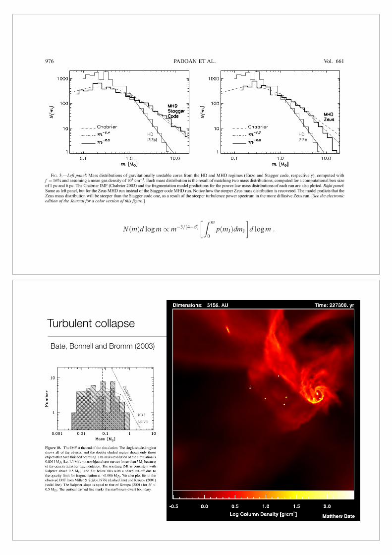
Fig. 4.—Time-averaged core mass distribution resulting from TVD simu-lations. The two dot-dashed lines with slopes of !0.5 and !1.3 are shown forcomparison with the mass functions of giant molecular clouds and protostellarcores, respectively.

Fig. 5.—Time-averaged core mass distribution resulting from SPH simu-lations. The two dot-dashed lines with slopes of !0.5 and !1.3 are shown forcomparison with the mass functions of giant molecular clouds and protostellarcores, respectively.

5 Even though we do not take the self-gravity of the gas into account, we givethe total mass in units of the Jeans mass. Other choices of the mass unit arepossible and fully equivalent. The reason for quoting the mass in Jeans masses isto allow for direct comparison with recent numerical works, (e.g., Klessen 2001;Gammie et al. 2003; Tilley& Pudritz 2004; Li et al. 2004), as well as with a futurecontribution of the analysis in the self-gravitating case. Note that we adopt a cubicdefinition of the Jeans mass,MJ " !k3. This differs from the spherical definition,MJ " 4"/3!(k/2)3, by a factor of #2.

BALLESTEROS-PAREDES ET AL.388 Vol. 637

THE STELLAR INITIAL MASS FUNCTION FROM TURBULENT FRAGMENTATION

Paolo PadoanJet Propulsion Laboratory, California Institute of Technology,MS 169-506, 4800 OakGrove Drive, Pasadena, CA 91109; padoan@ted.jpl.nasa.gov

and

Ake NordlundAstronomical Observatory and Theoretical Astrophysics Center, JulianeMaries Vej 30, DK-2100 Copenhagen, Denmark; aake@astro.ku.dk

Received 2000 November 25; accepted 2002May 15

ABSTRACT

The morphology and kinematics of molecular clouds (MCs) are best explained as the consequence ofsupersonic turbulence. Supersonic turbulence fragments MCs into dense sheets, filaments, and cores andlarge low-density ‘‘ voids,’’ via the action of highly radiative shocks. We refer to this process as turbulent frag-mentation.

In this work we derive the mass distribution of gravitationally unstable cores generated by the process ofturbulent fragmentation. The mass distribution above 1M! depends primarily on the power spectrum of theturbulent flow and on the jump conditions for isothermal shocks in a magnetized gas. For a power spectrumindex ! " 1:74, consistent with Larson’s velocity dispersion–size relation as well as with new numerical andanalytic results on supersonic turbulence, we obtain a power-lawmass distribution of dense cores with a slopeequal to 3=#4$ !% " 1:33, consistent with the slope of the stellar initial mass function (IMF). Below 1 M!,the mass distribution flattens and turns around at a fraction of 1 M!, as observed for the stellar IMF in anumber of stellar clusters, because only the densest cores are gravitationally unstable. The mass distributionat low masses is determined by the probability distribution of the gas density, which is known to be approxi-mately lognormal for an isothermal turbulent gas. The intermittent nature of the turbulent density distribu-tion is thus responsible for the existence of a significant number of small collapsing cores, even of substellarmass.

Since turbulent fragmentation is unavoidable in supersonically turbulent molecular clouds, and given thesuccess of the present model in predicting the observed shape of the stellar IMF, we conclude that turbulentfragmentation is essential to the origin of the stellar IMF.Subject headings: ISM: kinematics and dynamics — stars: formation —

stars: luminosity function, mass function — turbulence

1. INTRODUCTION

The process of star formation, particularly the origin ofthe stellar initial mass function (IMF), is a fundamentalproblem in astrophysics. Photometric properties and chemi-cal evolution of galaxies depend on their stellar content. Theprocess of galaxy formation cannot be described independ-ently of the process of star formation, since galaxies arepartly made of stars. Stars are also an important energysource for the interstellar medium (ISM) of galaxies.

Stars are formed in molecular clouds (MCs), which havebeen the focus of the research on star formation for morethan two decades. Currently, there is no generally acceptedtheory of star formation capable of predicting the star for-mation rate and the stellar IMF based on the physical prop-erties of MCs. This is hardly surprising, since turbulentmotions are ubiquitously observed in MCs, and the physicsof turbulence is poorly understood, because of the greatmathematical complexity of the fluid equations. Magneticfield, self-gravity, and high Mach numbers further increasethe complexity.

The steady growth of computer performance has nowmade large three-dimensional numerical simulations ofsupersonic magnetohydrodynamic (MHD) turbulence fea-sible (Padoan & Nordlund 1997, 1999; Stone, Ostriker, &Gammie 1998; Mac Low et al. 1998; Padoan, Zweibel, &Nordlund 2000; Klessen, Heitsch, & Mac Low 2000; MacLow & Ossenkopf 2000; Ostriker, Stone, & Gammie 2001;

Heitsch, Mac Low, & Klessen 2001; Padoan et al. 2001a,2001b). Comparisons of numerical experiments with obser-vational data have shown that supersonic turbulence canexplain the morphology and kinematics of MCs, and theformation of dense cores, provided that the motions are alsosuper-Alfvenic (Padoan, Jones, & Nordlund 1997a; Padoanet al. 1998, 1999, 2001a, 2001b; Padoan & Nordlund 1997,1999; Padoan, Rosolowsky, & Goodman 2001c). We referto this process of formation of dense cores inMCs by super-sonic turbulence as turbulent fragmentation. Since proto-stars evolve from the collapse of gravitationally unstablecores in MCs, even the stellar IMF could then be the resultof turbulent fragmentation, with the power-law shape of theIMF ultimately being the consequence of the self-similarnature of turbulence.

In this paper we do not use these increasingly sophisti-cated numerical simulations directly but instead develop ananalytic model. The assumptions of the model are inspiredby the qualitative properties of the numerical model, but thecurrent work does not depend on any particular set ofnumerical models or results.

Previous analytic models by Larson (1992), Henriksen(1986, 1991), and Elmegreen (1997, 1999, 2000b) havederived the stellar IMF on the basis of the self-similar struc-ture of MCs. Larson, assuming one-dimensional accretion,predicted a rather steep IMF slope, equal to the MC fractaldimension, while Henriksen found the IMF slope to dependon both the MC fractal dimension and the relation between

The Astrophysical Journal, 576:870–879, 2002 September 10# 2002. The American Astronomical Society. All rights reserved. Printed in U.S.A.

870

Once the physical size and mean density of the system arechosen, the CLUMPFIND algorithm depends only on two pa-rameters: (1) the spacing of the discrete density levels, f, and(2) the minimum density above which cores are selected, !min. Inprinciple, there is no need to define a minimum density, but inpractice it speeds up the algorithm. We have verified that results(including the total mass in cores) do not change significantly forvalues of !min below themean gas density, so we scan the densityfield only above the mean density. Notice that only half of thevolume, but most of the mass, is found above the mean density,because according to the lognormal pdf, most of the mass ispacked in a small volume fraction.

The parameter f may be chosen according to a physical modelproviding the value of the smallest density fluctuation that couldcollapse separately from its contracting background. However,given the difficulty of predicting the outcome of the gravitationalfragmentation, we prefer to simply search for a convergence of themass distribution with decreasing values of f. Luckily, the con-vergence is typically obtained already at a value of f ! 16%,meaning that differences between the mass distributions withf " 8% and 16% are generally insignificant. The cores are there-fore well defined, and in most cases they correspond to densityfluctuations, relative to the surrounding gas, even much largerthan f.

In the right panel of Figure 2, themass distributions above 1M#are plotted for themain four experiments, scaled to a mean densityof 104 cm$3, a box size of 6 pc, and a CLUMPFIND densityresolution f " 8%. Overplotted on the corresponding power-lawsection of eachmass distribution, the dashed lines show the powerlaw derived from the power-spectrum slope and the shock-jumpconditions of each simulation, according to the turbulent frag-mentation model, x " 3/(4$ " ) in the MHD regime and x "3/(5$ 2" ) in the HD regime. The general trend is recoveredwell, despite deviations to be expected because these mass dis-tributions are from single snapshots, not time averages.

The left panel of Figure 3 shows the mass distributions of theHD and MHD regimes (Enzo and Stagger code, respectively),computed with f " 16% and assuming a mean gas density of104 cm$3. Each mass distribution is the result of matching twomass distributions, computed for a computational box size of

1 pc and 6 pc. The 6 pc case makes it possible to sample massesin the range 1Y10 M# and hence to probe the effect of the tur-bulence power spectrum and shock-jump conditions on the massdistribution, but suffers from incompleteness for stars below 1M#.The 1 pc case samples well the turnover region and hence definesthe peak mass for that mean density and rms Mach number, butdoes not yield intermediate- and high-mass stars. The right panelof Figure 3 is equivalent to the left panel, but uses the MHD Zeusrun instead of the Stagger code run.The numerical mass distributions reproduce the sharp dif-

ference between the HD and MHD regimes predicted by theturbulent fragmentation model. The steeper mass distribution ex-pected from the Zeus run comparedwith the Stagger code run, dueto the steeper Zeus turbulence power spectrum, is also recovered.The slopes predicted by the turbulent fragmentation model areoverplotted in each figure. Furthermore, theMHD regime yields amass distribution of gravitationally unstable cores practicallyindistinguishable from Chabrier’s stellar IMF (Chabrier 2003),both in the Zeus and in the Stagger code runs. Finally, the Staggercode HD run also yields a mass distribution consistent with themodel prediction (see, e.g., the right panel of Fig. 2). The re-lation between the mass distribution and the power spectrumand shock-jump conditions is therefore successfully tested withthree different codes at very high numerical resolution. As dis-cussed below, the model predictions for the HD regime are alsoqualitatively confirmed with a fourth code (the total variation di-minishing [TVD] code) at lower resolution.To verify the convergence of the CLUMPFIND algorithm

with respect to the density resolution expressed by the parameter f,we plot in Figure 4 the mass distributions of the MHD regime,assuming a mean gas density of 104 cm$3 and a 6 pc size. Theleft panel is from the Stagger codeMHD run, and the right panelis from the ZeusMHD run. For this convergence study, we havecomputed together the mass distributions of unstable cores se-lected from three different snapshots.With these larger samples,statistical deviations are reduced, resulting in a more sensitivetest of convergence. Between f " 32% and f " 8%, there is atendency to fragment the largest cores and create a larger num-ber of small cores. However, the differences between f " 8%and f " 2% are rather small. Furthermore, the slope of the mass

Fig. 3.—Left panel: Mass distributions of gravitationally unstable cores from the HD and MHD regimes (Enzo and Stagger code, respectively), computed withf " 16% and assuming a mean gas density of 104 cm$3. Each mass distribution is the result of matching two mass distributions, computed for a computational box sizeof 1 pc and 6 pc. The Chabrier IMF (Chabrier 2003) and the fragmentation model predictions for the power-law mass distributions of each run are also plotted. Right panel:Same as left panel, but for the Zeus MHD run instead of the Stagger code MHD run. Notice how the steeper Zeus mass distribution is recovered. The model predicts that theZeus mass distribution will be steeper than the Stagger code one, as a result of the steeper turbulence power spectrum in the more diffusive Zeus run. [See the electronicedition of the Journal for a color version of this figure.]

PADOAN ET AL.976 Vol. 661

respect toMach numbers and average gas density) but inter-preted at di!erent scales L1 and L2 > L1. The total mass inthe ‘‘ large-scale ’’ experiment is obviously !L2=L1"3 largerthan in the ‘‘ small-scale ’’ experiment. The cores in thelarge-scale experiment would be equal in number but heav-ier by the ratio !L2=L1"3 than cores in the small-scale experi-ment. On the other hand, the total number of cores in thesmall-scale experiment is !L2=L1"3 larger than in the large-scale experiment if the same total mass is used in the twocases [i.e., if cores from a number !L2=L1"3 of small-scaleexperiments are counted together]. The result is therefore atotal number of cores that depends on scale as

N / L#3 ; !17"

in agreement with Elmegreen’s (1997) result.When the Mach number dependence on scale is taken

into account, the result is that the larger scales contributerelatively less massive cores because of the scaling relation(14). We assume that the number of cores per scale L stillscales as L#3. Combining the relations (14) and (17) weobtain

N!m"d logm / m#3=!4#!"d logm : !18"

If the spectral index is consistent with the observed velocitydispersion–size Larson relation (Larson 1981) and with ournumerical and analytical results (Boldyrev et al. 2002), then! $ 1:74 and the mass distribution is

N!m"d logm / m#1:33d logm ; !19"

which is almost identical to the Salpeter stellar IMF (Sal-peter 1955).

6. THE MASS DISTRIBUTION OFCOLLAPSING CORES

The mass distribution of dense cores has been computedassuming that the preshock density is n0 and the postshockdensityMAn0, whereMA is scale dependent. Amore precisecomputation should include the e!ect of the probability dis-tribution of the value of MA at each scale, or the overalle!ect of the statistics of the turbulent velocity field, which isthe generation of a lognormal PDF of mass density (see x 4).This is necessary to compute the fraction of dense cores thatare gravitationally unstable and collapse into protostars,since dense cores can be significantly denser than their aver-age density predicted by the scaling laws. While most of thelarge cores will be dense enough to collapse, the probabilitythat small cores are dense enough to collapse is determinedby the PDF of mass density. Because of the intermittentnature of the lognormal PDF, even very small (substellar)cores have a finite chance to be dense enough to collapse.

We write the thermal Jeans mass as

mJ $ mJ; 0n

n0

! "#1=2

; !20"

where

mJ; 0 $ 1:2 M%T

10 K

! "3=2! n01000 cm#3

"#1=2

!21"

is the Jeans mass at the mean density n0. The distribution ofthe Jeans mass is obtained from the PDF of density assum-

ing constant temperature as in Padoan et al. (1997b):

p!mJ"d lnmJ $1######

2"p

#=2

mJ

mJ; 0

! "#2

& exp # 1

2

lnmJ # A

#=2

! "2" #

d lnmJ ; !22"

wheremJ is in solar masses and

A $ lnm2J; 0 # ln n0 : !23"

The fraction of cores of mass m with gravitational energy inexcess of their thermal energy is given by the integral ofp!mJ" from 0 tom. The mass distribution of collapsing coresis therefore

N!m"d logm / m#3=!4#!"Z m

0p!mJ"dmJ

$ %d logm : !24"

The mass distribution is plotted in Figure 1, for ! $ 1:8.In the top panel the mass distribution is computed for threedi!erent values of the largest turbulent scale L0, assumingLarson-type relations (Larson 1981) to rescale n0 and MA; 0

according to the value of L0. The mass distribution is apower law, determined by the power spectrum of turbu-lence, for masses larger than approximately 1 M%. Atsmaller masses the mass distribution flattens, reaches a max-imum at a fraction of 1 M%, and then decreases withdecreasing stellar mass. Collapsing substellar masses arefound, thanks to the intermittent density distribution in theturbulent flow. The middle and bottom panels of Figure 1show the dependence of the mass distribution on the rmsMach number of the flow and on the average gas density,respectively.

The magnetic critical mass is derived in the next section.We have not used it here to obtain the mass distribution ofcollapsing cores because the thermal Jeans mass is a morestrict condition for collapse. The magnetic critical massdepends on the core morphology in relation to the fieldgeometry and on the magnetic field strength that correlateswith the gas density with a very large scatter (see below). Itis possible therefore that magnetic pressure support againstthe gravitational collapse a!ects the shape of the mass distri-bution but only as a secondary e!ect.

7. THE STELLAR IMF

Observations show that the stellar IMF is a power lawabove 1–2 M%, with exponent around the Salpeter valuex $ 1:35, roughly independent of environment (Elmegreen1998, 2001); gradually flattens at smaller masses; and peaksat approximately 0.2–0.6M% (Hillenbrand 1997; Bouvier etal. 1998; Luhman 1999, 2000; Luhman & Rieke 1999; Luh-man et al. 2000). The shape of the IMF below 1–2 M%, andparticularly the relative abundance of brown dwarfs, maydepend on the physical environment (Luhman 2000).

The scalings discussed above result in a mass distributionof dense cores consistent with the stellar IMF for masseslarger than 1M%, without invoking a sampling rate propor-tional to the free-fall time, or ‘‘ competition for mass ’’ as inElmegreen (1997, 1999). Two conclusions are possible:either there are e!ects in addition to those considered byElmegreen and they all happen to cancel each other, or elseadditional e!ects are not important in the first place. In the

874 PADOAN & NORDLUND Vol. 576

Bate, Bonnell and Bromm (2003)

Turbulent collapse

2003MNRAS.339..577B

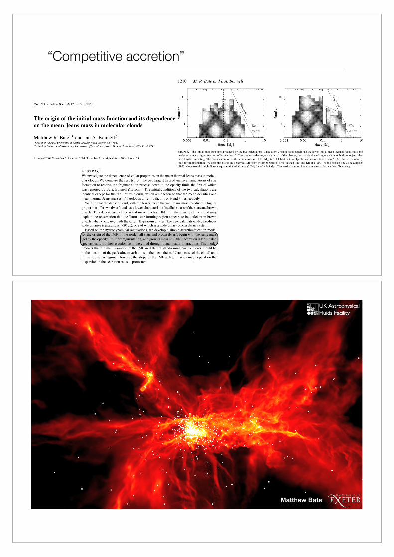
“Competitive accretion”

2005MNRAS.356.1201B

2005MNRAS.356.1201B

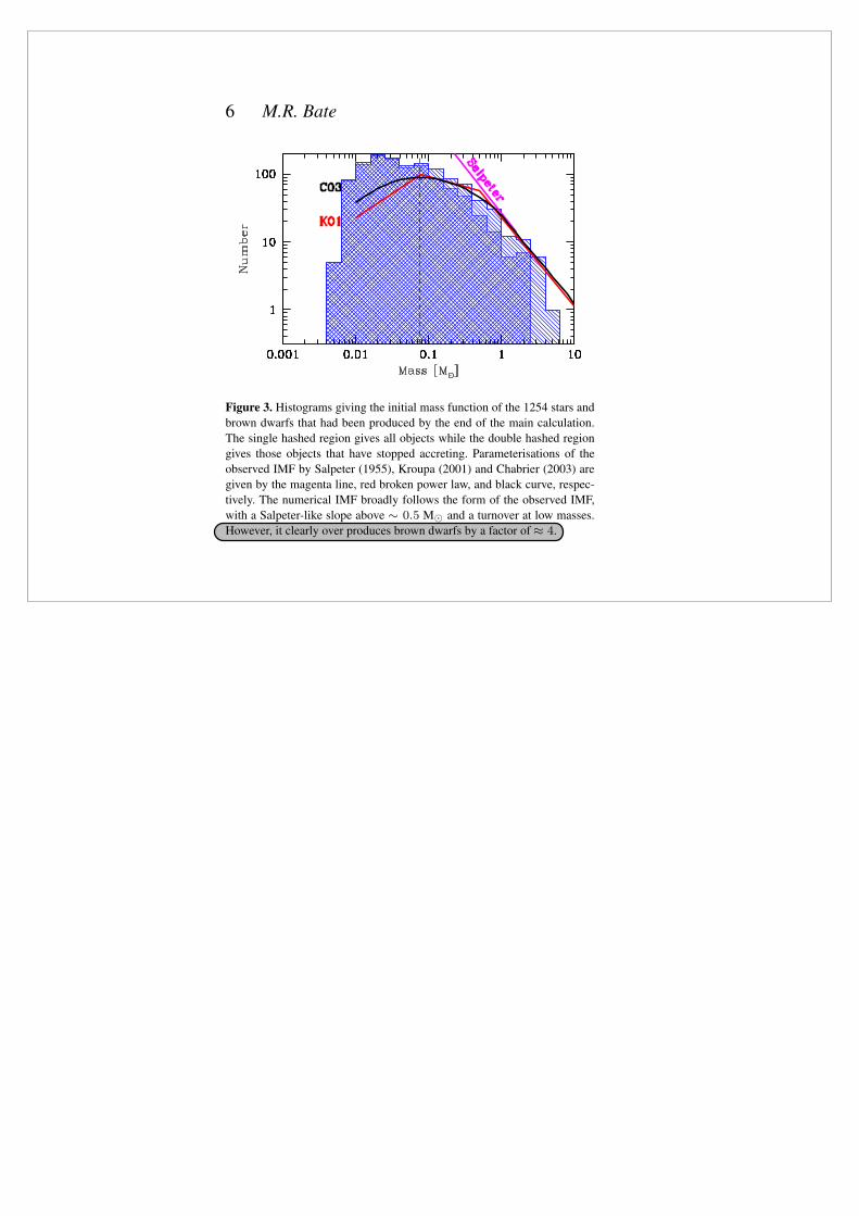
6 M.R. Bate

Figure 3. Histograms giving the initial mass function of the 1254 stars and

brown dwarfs that had been produced by the end of the main calculation.

The single hashed region gives all objects while the double hashed region

gives those objects that have stopped accreting. Parameterisations of the

observed IMF by Salpeter (1955), Kroupa (2001) and Chabrier (2003) are

given by the magenta line, red broken power law, and black curve, respec-

tively. The numerical IMF broadly follows the form of the observed IMF,

with a Salpeter-like slope above ∼ 0.5 M⊙ and a turnover at low masses.

However, it clearly over produces brown dwarfs by a factor of≈ 4.

BBB2003, BB2005, B2005. Figure 1 shows snapshots of column

density from the main calculation illustrating the global evolu-

tion. The initial turbulent velocity field generates structures with

those that are strongly self-gravitating collapsing to form stellar

groups and clusters. The main difference from the earlier calcula-

tions is that with such a large cloud at least 5 sub-clusters contain-

ing dozens to hundreds of objects form (t ≈ 1.10 − 1.20tff ), and

then merge together to form a single dense stellar cluster by the end

of the calculation. Such hierarchical build-up of a stellar cluster was

previously highlighted in the lower-resolution simulation of a 1000

M⊙ cloud performed by Bonnell et al. (2003). The evolution of

the cloud and the formation and merger of the sub-clusters is best

viewed in a animation. Animations of the main calculation can be

downloaded from http://www.astro.ex.ac.uk/people/mbate/Cluster/

in both the colour scheme of Figure 1 and as a 3-D red-cyan movie.

Unfortunately, the resolved circumstellar discs and binary systems

are not visible on the scale of Figure 1, however, with well over

100 multiple systems it is impossible to display these in a paper.

In Figure 2 we display the global evolution of the re-run calcula-

tion. There are no substantial differences on large-scales between

the two calculations, with the exception of the different pattern of

ejected objects visible at t = 1.00tff (c.f. the two panels in Fig-

ures 1 and 2). Since the dynamics of individual stellar systems is

chaotic, even changing the sink particle parameters on very small

scales affects the outcomes of dynamical interactions. In the fol-

lowing subsections of the paper, we examine the statistical proper-

ties of the stellar systems.

3.1 The initial mass function

The initial mass function produced by the end of the main calcu-

lation is shown in Figure 3 and is compared with the parameter-

isations of the observed IMF given by Chabrier (2003), Kroupa

(2001), and Salpeter (1955). The IMFs obtained from BBB2003

and B2005 were, within the statistical uncertainties, consistent

with the observed IMF. However, the IMF from the main calcu-

lation reported on here is much more accurately determined and is

clearly not consistent with the observed IMF. The computed IMF

has a similar overall form to the observed IMF, with a reasonable

Salpeter-type slope at the high-mass end, a flattening below a solar-

mass, and an eventual turn over. However, it significantly over pro-

duces brown dwarfs. The calculation produces 459 stars and 795

brown dwarfs (masses < 0.075 M⊙). Even taking into account that

46 of the brown dwarfs are still accreting when the calculation is

stopped and may eventually reach stellar masses, the ratio of brown

dwarfs to stars is at least 3:2 whereas recent observations suggest

that the IMF produces more stars than brown dwarfs (Greissl et al.

2007; Andersen et al. 2008). Andersen et al. (2008) find that the ra-

tio of stars with masses 0.08−1.0 M⊙ to brown dwarfs with masses

0.03− 0.08 M⊙ is N(0.08− 1.0)/N(0.03− 0.08) ≈ 5± 2. For

the main calculation, this ratio is 408/326 = 1.25. Although the

IMF below 0.03 M⊙ is not yet well constrained observationally the

number of objects seems to be decreasing for lower masses. Thus,

it is unlikely that the true ratio of brown dwarfs to stars exceeds

1:3. The main calculation, therefore, over produces brown dwarfs

relative to stars by a factor of≈ 4 compared with the observed IMF.

3.1.1 The dependence of the IMF on numerical approximationsand missing physics

There are several potential causes of brown dwarf over production

that may be divided into two categories: numerical effects or ne-

glected physical processes. Arguably, the main numerical approx-

imation made in the calculations is that of sink particles. High-

density gas is replaced by a sink particle whenever the maximum

density exceeds 10−10g cm

−3and the gas within a radius of 5

AU is accreted onto the sink particle producing a gravitating point

mass containing a few Jupiter masses of material. These sink parti-

cles then interact with each other ballistically, which, for example,

might plausibly artificially enhance ejections and the production of

low-mass objects.

In order to investigate the effect of the sink particle approxi-

mation on the results, we re-ran part of the main calculation with

smaller sink particles (accretion radii of 0.5 AU) and without grav-

itational softening between sink particles (they were allowed to

merge if them came within 4 R⊙ of each other). This calculation

was only followed to 1.038 tff due to its much more time consum-

ing nature. The small accretion radius calculation produced 258

stars and brown dwarfs in the same time period that the main cal-

culation produced 221 objects. Because the calculations are chaotic

identical results should not be expected. The main question to an-

swer is whether or not the results are statistically different.

In Figures 4 and 5 we compare the IMFs produced by the main

calculation and the smaller sink particle calculation at the same

time. The smaller sink particle calculation produces twice as many

objects with masses less than 10 Jupiter masses than the main cal-

culation, but overall the two IMFs are very similar. A K-S test run

on the two distributions shows that they have a 13% probability

of being drawn from the same underlying IMF (i.e. they are sta-

tistically indistinguishable). Removing objects with less than 10

Jupiter-masses from the K-S test results in a 38% probability of

the two distributions being drawn from the same underlying IMF.

We conclude that variations in the sink particle accretion radii and

gravitational softening may have an effect on the production of ex-

tremely low-mass objects. However, changes to the sink particle

parameters do not significantly alter the overall results and, thus,

the use of sink particles is probably not responsible for the signifi-

cant over production of brown dwarfs.

It seems most likely that the over production of brown dwarfs

c� 0000 RAS, MNRAS 000, 000–000