EnMAP Field Guides - gfz-potsdam.degfzpublic.gfz-potsdam.de/pubman/item/escidoc:1381850/component/... · Instruments for LAI measurements with this method are the SunSCAN of Delta-T

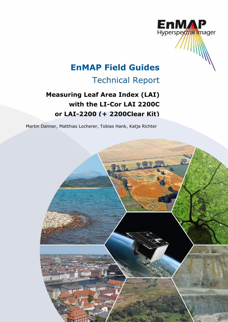
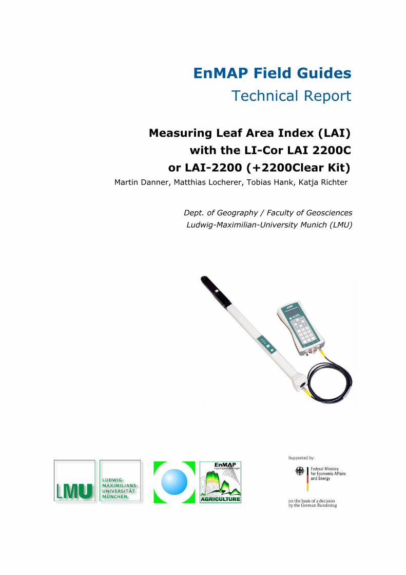
Measuring Leaf Area Index (LAI)

with the LI-Cor LAI 2200C

or LAI-2200 (+ 2200Clear Kit)

EnMAP Field Guides

Technical Report

Martin Danner, Matthias Locherer, Tobias Hank, Katja Richter

Recommended citation:

Danner, M.; Locherer, M.; Hank, T.; Richter, K. (2015): Measuring Leaf Area Index

(LAI) with the LI-Cor LAI 2200C or LAI-2200 (+2200Clear Kit) –

Theory, Measurement, Problems, Interpretation. EnMAP Field Guide Technical Report, GFZ Data Services. DOI: http://doi.org/10.2312/enmap.2015.009

Imprint

EnMAP Consortium

GFZ Data Services

Telegrafenberg

D-14473 Potsdam

Published in Potsdam, Germany

October 2015

http://doi.org/10.2312/enmap.2015.009

http://doi.org/

http://doi.org/10.2312/enmap.2015.009

https://creativecommons.org/licenses/by-sa/4.0/

Measuring Leaf Area Index (LAI)

with the LI-Cor LAI 2200C

EnMAP Field Guides

Technical Report

or LAI-2200 (+2200Clear Kit)

Martin Danner, Matthias Locherer, Tobias Hank, Katja Richter

Dept. of Geography / Faculty of Geosciences

Ludwig-Maximilian-University Munich (LMU)

Table of contents

Table of contents ..................................................................................................................................

List of Figures ........................................................................................................................................

List of Tables..........................................................................................................................................

1 Introduction .................................................................................................................................... 1

1.1 Definitions ............................................................................................................................... 1

1.2 Areas of Application ................................................................................................................ 1

1.3 Measurement and Devices ...................................................................................................... 1

2 Data Collection ............................................................................................................................... 2

2.1 Theory: Measurement Principle .............................................................................................. 2

2.2 Technical Accomplishment ...................................................................................................... 3

2.2.1 LAI Setup .......................................................................................................................... 3

2.2.2 Getting started ................................................................................................................ 5

2.2.3 Technical settings ............................................................................................................ 5

2.2.4 Measurement .................................................................................................................. 8

2.3 Sampling Strategy .................................................................................................................... 9

2.4 Sources of Errors and Uncertainties ...................................................................................... 15

3 Data Elaboration ........................................................................................................................... 15

3.1 Required Software ................................................................................................................. 15

3.2 Data Output & Correction Methods ...................................................................................... 16

4 References .................................................................................................................................... 19

5 Appendix ....................................................................................................................................... 20

List of Figures

Figure 2-1: Schematic composition of the LI-Cor PCA LAI-2200 sensor (LI-Cor, 2009). ........................ 3

Figure 2-2: The Control Panel on a LI-Cor LAI-2200’s sensor arm. ....................................................... 4

Figure 2-3: Operating procedure of LAI measurements for densely grown row crops (LI-Cor, 2009).

.......................................................................................................................................... 12

Figure 2-4: Operating procedure of LAI measurements for sparsely grown row crops (LI-Cor, 2009).

.......................................................................................................................................... 13

List of Tables

Table 2-1: Selectable parameters to be indicated on the console’s display (LI-Cor, 2009)................. 5

Table 2-2: Amount of B readings to be taken, in dependence of the SEL/LAI ratio (LI-Cor, 2009). .. 10

Table 2-3: Distance factors for an estimation of the minimum distance to leaves, depending on the

View Cap in use (LI-Cor, 2009). ......................................................................................... 11

Table 3-1: Selection of generated output files after computation of the LAI is done (LI-Cor, 2009) 16

EnMAP Field Guides: LI-Cor LAI - doi:10.2312/enmap.2015.009 1

1 Introduction

1.1 Definitions

Leaf area index, LAI, is one of the most important parameters for canopy architecture. According to a

common definition it quantifies the one-sided area of leaf surface per unit of horizontal ground area

(Watson, 1947). Difficulties arise, however, when trying to apply this definition to needles or other

non-flat leafs. A more accurate description is given by Chen & Black (1992), characterizing the LAI as

half of the area of completely evolved leafs per unit of horizontal ground area, thus making it

independent of geometrical leaf attributes. As a dimensionless factor, this parameter describes the

overall leaf area of a canopy with vertical extent to the corresponding size of ground, e.g. m² per m².

1.2 Areas of Application

The leaf area index is of upmost importance for eco-physiology in many ways: in modelling, it serves

as a scaling factor, controlling processes like photosynthesis and evapotranspiration (Weiss et al.,

2004; Bréda, 2003). Acting as transition zone between plant and atmosphere, most processes of gas

and water exchange as well as the interception of rain water, take place on the surface of leaves

(Bréda, 2003). By extinction of incident radiation, variations in the LAI influence the micro climate

within and above the canopy (Welles, 1990). Combining the leaf area parameter with information

about the distribution of leaf angles, it is possible to model the amount of absorbed photosynthetically

active radiation APAR. In the course of a ground data campaign, measurements of the LAI play a crucial

role for the calibration and validation of remote sensing data.

1.3 Measurement and Devices

There is a general distinction between direct and indirect methods. Direct methods are mostly based

on a specific relation between leaf surface areas per norm area. Classed as a planimetrical approach,

the accuracy of this method makes it ideal for the calibration and validation of other methods (Bréda,

2003). The gravimetric procedures deserve additional recognition: dry mass and leaf area of a single

leaf are determined and then their ratio is assigned to any amount of foliage (Daughtry, 1990). Since

both layouts require laboratory treatment, a destructive procedure in the field is inevitable. Overall,

direct methods are more precise, but also time consuming and hence a suboptimal choice for long

term studies. In addition, already analyzed plant material will be missing in each consequent

observation, distorting LAI values more and more during the course of the campaign (Jonckheere,

2004).

Making use of indirect methods, LAI can be determined in situ without withdrawal of biomass.

Information about foliage density and extent are derived by measurements of reflected or transmitted

radiation either within or beneath the canopy. Despite the fact that sources of errors do occur

inevitably when a parameter is not measured directly, these indirect methods have become popular

and scientifically accepted due to their speed and straightforwardness. A possible way to deduce the


LAI from indirect measurements is the usage of models treating the canopy as a homogeneous turbid

medium. They dilute irradiation accordant to an extinction coefficient k, i.e. inversion of the Beer-

Lambert extinction by Monsi & Saeki (1953).

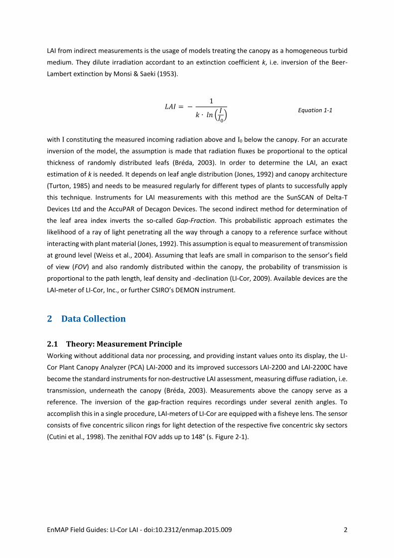
𝐿𝐴𝐼 = − 1

𝑘 ∙ 𝑙𝑛 (𝐼𝐼0

)

Equation 1-1

with I constituting the measured incoming radiation above and I0 below the canopy. For an accurate

inversion of the model, the assumption is made that radiation fluxes be proportional to the optical

thickness of randomly distributed leafs (Bréda, 2003). In order to determine the LAI, an exact

estimation of k is needed. It depends on leaf angle distribution (Jones, 1992) and canopy architecture

(Turton, 1985) and needs to be measured regularly for different types of plants to successfully apply

this technique. Instruments for LAI measurements with this method are the SunSCAN of Delta-T

Devices Ltd and the AccuPAR of Decagon Devices. The second indirect method for determination of

the leaf area index inverts the so-called Gap-Fraction. This probabilistic approach estimates the

likelihood of a ray of light penetrating all the way through a canopy to a reference surface without

interacting with plant material (Jones, 1992). This assumption is equal to measurement of transmission

at ground level (Weiss et al., 2004). Assuming that leafs are small in comparison to the sensor’s field

of view (FOV) and also randomly distributed within the canopy, the probability of transmission is

proportional to the path length, leaf density and -declination (LI-Cor, 2009). Available devices are the

LAI-meter of LI-Cor, Inc., or further CSIRO’s DEMON instrument.

2 Data Collection

2.1 Theory: Measurement Principle

Working without additional data nor processing, and providing instant values onto its display, the LI-

Cor Plant Canopy Analyzer (PCA) LAI-2000 and its improved successors LAI-2200 and LAI-2200C have

become the standard instruments for non-destructive LAI assessment, measuring diffuse radiation, i.e.

transmission, underneath the canopy (Bréda, 2003). Measurements above the canopy serve as a

reference. The inversion of the gap-fraction requires recordings under several zenith angles. To

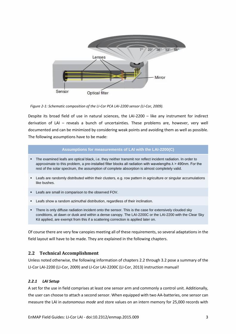
accomplish this in a single procedure, LAI-meters of LI-Cor are equipped with a fisheye lens. The sensor

consists of five concentric silicon rings for light detection of the respective five concentric sky sectors

(Cutini et al., 1998). The zenithal FOV adds up to 148° (s. Figure 2-1).


Figure 2-1: Schematic composition of the LI-Cor PCA LAI-2200 sensor (LI-Cor, 2009).

Despite its broad field of use in natural sciences, the LAI-2200 – like any instrument for indirect

derivation of LAI – reveals a bunch of uncertainties. These problems are, however, very well

documented and can be minimized by considering weak points and avoiding them as well as possible.

The following assumptions have to be made:

Assumptions for measurements of LAI with the LAI-2200(C)

The examined leafs are optical black, i.e. they neither transmit nor reflect incident radiation. In order to

approximate to this problem, a pre-installed filter blocks all radiation with wavelengths λ > 490nm. For the

rest of the solar spectrum, the assumption of complete absorption is almost completely valid.

Leafs are randomly distributed within their clusters, e.g. row pattern in agriculture or singular accumulations

like bushes.

Leafs are small in comparison to the observed FOV.

Leafs show a random azimuthal distribution, regardless of their inclination.

There is only diffuse radiation incident onto the sensor. This is the case for extensively clouded sky

conditions, at dawn or dusk and within a dense canopy. The LAI-2200C or the LAI-2200 with the Clear Sky

Kit applied, are exempt from this if a scattering correction is applied later on.

Of course there are very few canopies meeting all of these requirements, so several adaptations in the

field layout will have to be made. They are explained in the following chapters.

2.2 Technical Accomplishment

Unless noted otherwise, the following information of chapters 2.2 through 3.2 pose a summary of the

LI-Cor LAI-2200 (LI-Cor, 2009) and LI-Cor LAI-2200C (LI-Cor, 2013) instruction manual!

2.2.1 LAI Setup

A set for the use in field comprises at least one sensor arm and commonly a control unit. Additionally,

the user can choose to attach a second sensor. When equipped with two AA-batteries, one sensor can

measure the LAI in autonomous mode and store values on an intern memory for 25,000 records with


a maximum operation time of 8 hours. For the attached mode, no batteries are needed in the sensor

arm. The console, however, needs to be powered by 4 AA-batteries, providing electricity for up to 80

hours with one sensor attached and in use. Storage of the console is managed by a 128MB SD-card.

Note: Do not exchange the intern SD-card by any other memory than one

distributed by LI-Cor, Inc.!

Console and sensor arms as well as different View Caps for restriction of the azimuthal FOV, USB data

cables, optical data cables for the connection between console and arms, and a lens cleaning set, are

all to be stored in the LI-Cor case for field use.

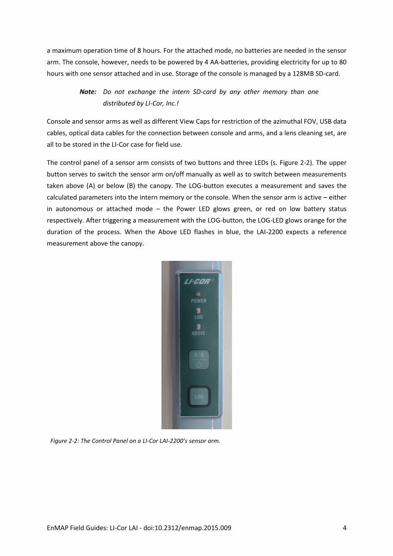
The control panel of a sensor arm consists of two buttons and three LEDs (s. Figure 2-2). The upper

button serves to switch the sensor arm on/off manually as well as to switch between measurements

taken above (A) or below (B) the canopy. The LOG-button executes a measurement and saves the

calculated parameters into the intern memory or the console. When the sensor arm is active – either

in autonomous or attached mode – the Power LED glows green, or red on low battery status

respectively. After triggering a measurement with the LOG-button, the LOG-LED glows orange for the

duration of the process. When the Above LED flashes in blue, the LAI-2200 expects a reference

measurement above the canopy.

Figure 2-2: The Control Panel on a LI-Cor LAI-2200’s sensor arm.


2.2.2 Getting started

Correct placement and treatment of important components

(1) If desired, connect one or two sensor arm(s) to the console at linkage X or/and Y. The connectors

labelled ‘1’ and ‘2’ are for optional LI-Cor Biosciences Quantum sensors (LI-190 or LI-191),

pyranometers (LI-200) or photometric sensors (LI-219) for measurements of photosynthetically active

radiation. They will not be discussed in this field guide.

(2) Remove the protective View Cap from the sensor and, if necessary, replace it by a narrowed one for

your individual sampling strategy (s. 2.3). Before you do so, you can check the lens for dirt and clean it

safely with distilled water and a cloth.

“Note: Be very careful not to scratch the MgF2 coating on the lens. Avoid cleaning the lens with paper

products, and never wipe the lens while it is dry. Damage to the lens is not covered under warranty.”

(LI-Cor, 2009)

(3) For measurements in the field, it may be convenient to attach the snap hook to your pants’ belt or bail.

(4) Once the setup is ready, press the Power button on the console and apply all necessary settings

relevant for your field project.

2.2.3 Technical settings

In the console menu you will be able to view and edit different kinds of settings. For some projects the

pre-defined parameters will work fine, but the more precise you choose variables and methods, the

better your results will be. Depending on the methodological approach in the field, you can choose to

change (a) the display mode, (b) technical parameters, (c) the way radiance measurements are to be

taken and (d) the way a LAI file is computed out of the radiance measurements.

a) Display mode

When switched on, the console indicates four parameters on the display. Navigate through these

parameters with the ↑↓ arrows and change them by pressing ← or →.

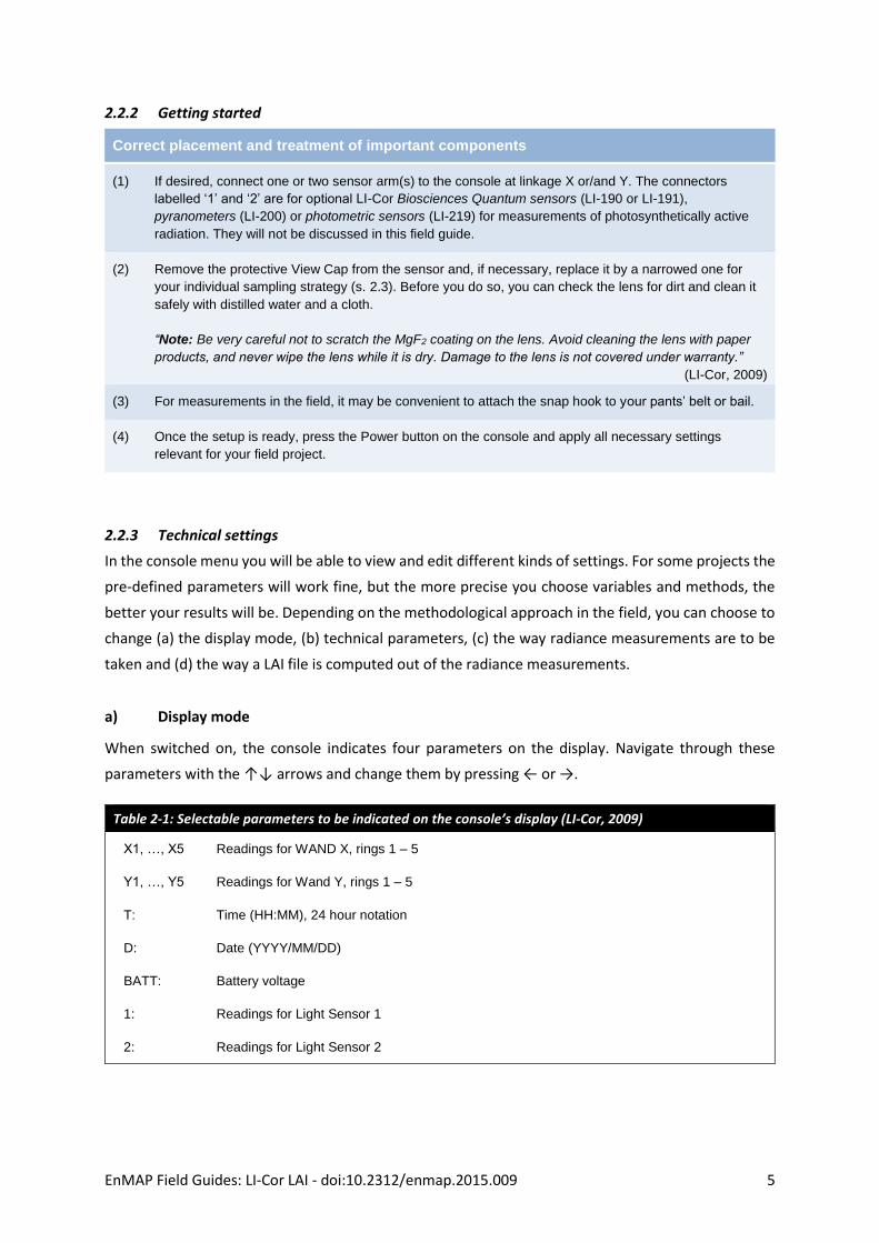
Table 2-1: Selectable parameters to be indicated on the console’s display (LI-Cor, 2009)

X1, …, X5 Readings for WAND X, rings 1 – 5

Y1, …, Y5 Readings for Wand Y, rings 1 – 5

T: Time (HH:MM), 24 hour notation

D: Date (YYYY/MM/DD)

BATT: Battery voltage

1: Readings for Light Sensor 1

2: Readings for Light Sensor 2


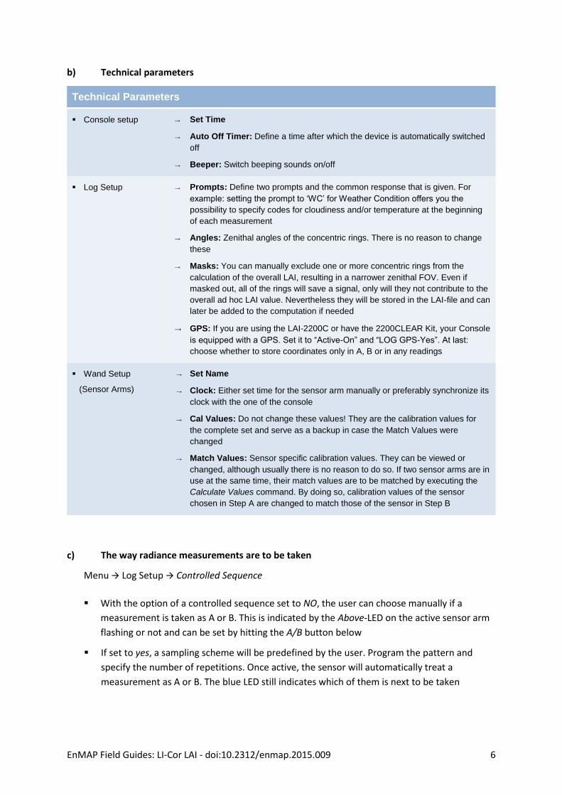
b) Technical parameters

Technical Parameters

Console setup → Set Time

→ Auto Off Timer: Define a time after which the device is automatically switched

off

→ Beeper: Switch beeping sounds on/off

Log Setup → Prompts: Define two prompts and the common response that is given. For

example: setting the prompt to ‘WC’ for Weather Condition offers you the

possibility to specify codes for cloudiness and/or temperature at the beginning

of each measurement

→ Angles: Zenithal angles of the concentric rings. There is no reason to change

these

→ Masks: You can manually exclude one or more concentric rings from the

calculation of the overall LAI, resulting in a narrower zenithal FOV. Even if

masked out, all of the rings will save a signal, only will they not contribute to the

overall ad hoc LAI value. Nevertheless they will be stored in the LAI-file and can

later be added to the computation if needed

→ GPS: If you are using the LAI-2200C or have the 2200CLEAR Kit, your Console

is equipped with a GPS. Set it to “Active-On” and “LOG GPS-Yes”. At last:

choose whether to store coordinates only in A, B or in any readings

Wand Setup

(Sensor Arms)

→ Set Name

→ Clock: Either set time for the sensor arm manually or preferably synchronize its

clock with the one of the console

→ Cal Values: Do not change these values! They are the calibration values for

the complete set and serve as a backup in case the Match Values were

changed

→ Match Values: Sensor specific calibration values. They can be viewed or

changed, although usually there is no reason to do so. If two sensor arms are in

use at the same time, their match values are to be matched by executing the

Calculate Values command. By doing so, calibration values of the sensor

chosen in Step A are changed to match those of the sensor in Step B

c) The way radiance measurements are to be taken

Menu Log Setup Controlled Sequence

With the option of a controlled sequence set to NO, the user can choose manually if a

measurement is taken as A or B. This is indicated by the Above-LED on the active sensor arm

flashing or not and can be set by hitting the A/B button below

If set to yes, a sampling scheme will be predefined by the user. Program the pattern and

specify the number of repetitions. Once active, the sensor will automatically treat a

measurement as A or B. The blue LED still indicates which of them is next to be taken


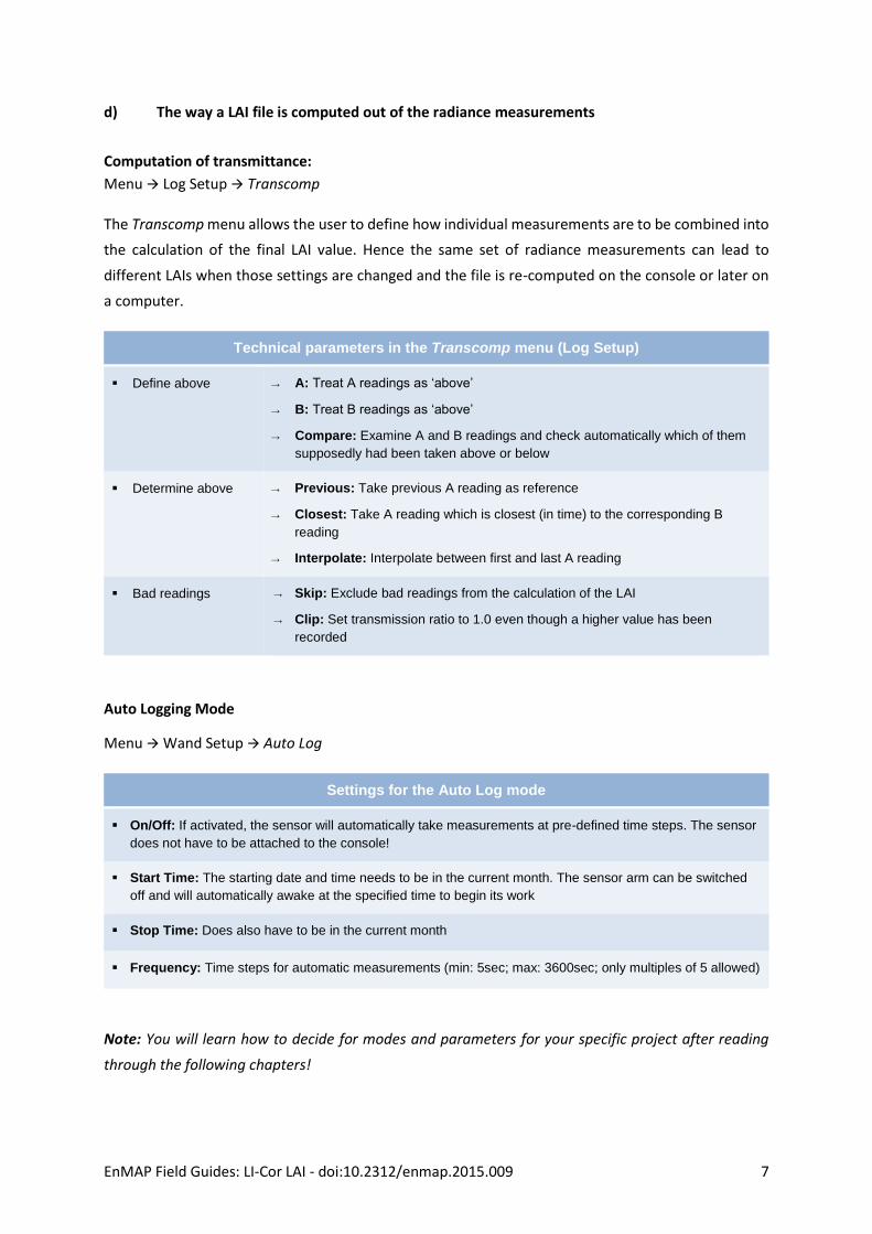
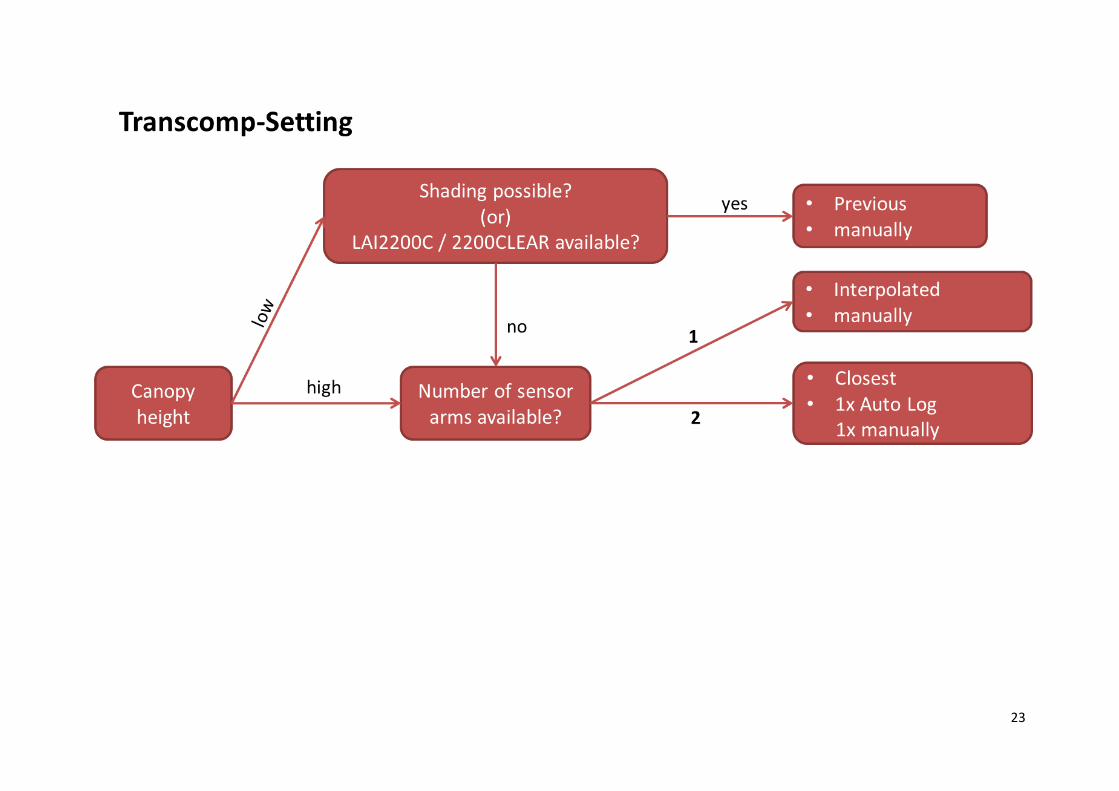
d) The way a LAI file is computed out of the radiance measurements

Computation of transmittance:

Menu Log Setup Transcomp

The Transcomp menu allows the user to define how individual measurements are to be combined into

the calculation of the final LAI value. Hence the same set of radiance measurements can lead to

different LAIs when those settings are changed and the file is re-computed on the console or later on

a computer.

Technical parameters in the Transcomp menu (Log Setup)

Define above → A: Treat A readings as ‘above’

→ B: Treat B readings as ‘above’

→ Compare: Examine A and B readings and check automatically which of them

supposedly had been taken above or below

Determine above → Previous: Take previous A reading as reference

→ Closest: Take A reading which is closest (in time) to the corresponding B

reading

→ Interpolate: Interpolate between first and last A reading

Bad readings

→ Skip: Exclude bad readings from the calculation of the LAI

→ Clip: Set transmission ratio to 1.0 even though a higher value has been

recorded

Auto Logging Mode

Menu Wand Setup Auto Log

Settings for the Auto Log mode

On/Off: If activated, the sensor will automatically take measurements at pre-defined time steps. The sensor

does not have to be attached to the console!

Start Time: The starting date and time needs to be in the current month. The sensor arm can be switched

off and will automatically awake at the specified time to begin its work

Stop Time: Does also have to be in the current month

Frequency: Time steps for automatic measurements (min: 5sec; max: 3600sec; only multiples of 5 allowed)

Note: You will learn how to decide for modes and parameters for your specific project after reading

through the following chapters!


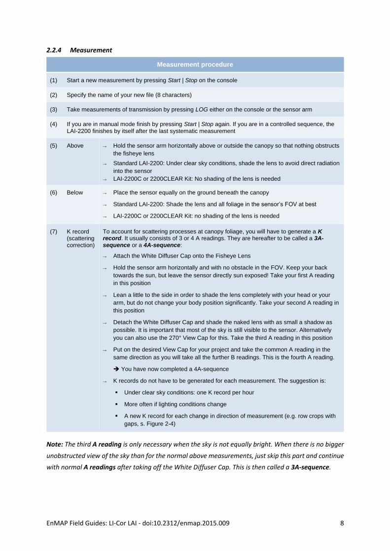
2.2.4 Measurement

Measurement procedure

(1) Start a new measurement by pressing Start | Stop on the console

(2) Specify the name of your new file (8 characters)

(3) Take measurements of transmission by pressing LOG either on the console or the sensor arm

(4) If you are in manual mode finish by pressing Start | Stop again. If you are in a controlled sequence, the

LAI-2200 finishes by itself after the last systematic measurement

(5) Above → Hold the sensor arm horizontally above or outside the canopy so that nothing obstructs

the fisheye lens

→ Standard LAI-2200: Under clear sky conditions, shade the lens to avoid direct radiation

into the sensor

→ LAI-2200C or 2200CLEAR Kit: No shading of the lens is needed

(6) Below → Place the sensor equally on the ground beneath the canopy

→ Standard LAI-2200: Shade the lens and all foliage in the sensor’s FOV at best

→ LAI-2200C or 2200CLEAR Kit: no shading of the lens is needed

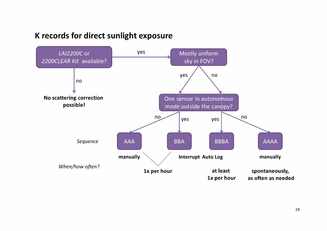
(7) K record (scattering correction)

To account for scattering processes at canopy foliage, you will have to generate a K record. It usually consists of 3 or 4 A readings. They are hereafter to be called a 3A-sequence or a 4A-sequence:

→ Attach the White Diffuser Cap onto the Fisheye Lens

→ Hold the sensor arm horizontally and with no obstacle in the FOV. Keep your back

towards the sun, but leave the sensor directly sun exposed! Take your first A reading

in this position

→ Lean a little to the side in order to shade the lens completely with your head or your

arm, but do not change your body position significantly. Take your second A reading in

this position

→ Detach the White Diffuser Cap and shade the naked lens with as small a shadow as

possible. It is important that most of the sky is still visible to the sensor. Alternatively

you can also use the 270° View Cap for this. Take the third A reading in this position

→ Put on the desired View Cap for your project and take the common A reading in the

same direction as you will take all the further B readings. This is the fourth A reading.

You have now completed a 4A-sequence

→ K records do not have to be generated for each measurement. The suggestion is:

Under clear sky conditions: one K record per hour

More often if lighting conditions change

A new K record for each change in direction of measurement (e.g. row crops with

gaps, s. Figure 2-4)

Note: The third A reading is only necessary when the sky is not equally bright. When there is no bigger

unobstructed view of the sky than for the normal above measurements, just skip this part and continue

with normal A readings after taking off the White Diffuser Cap. This is then called a 3A-sequence.


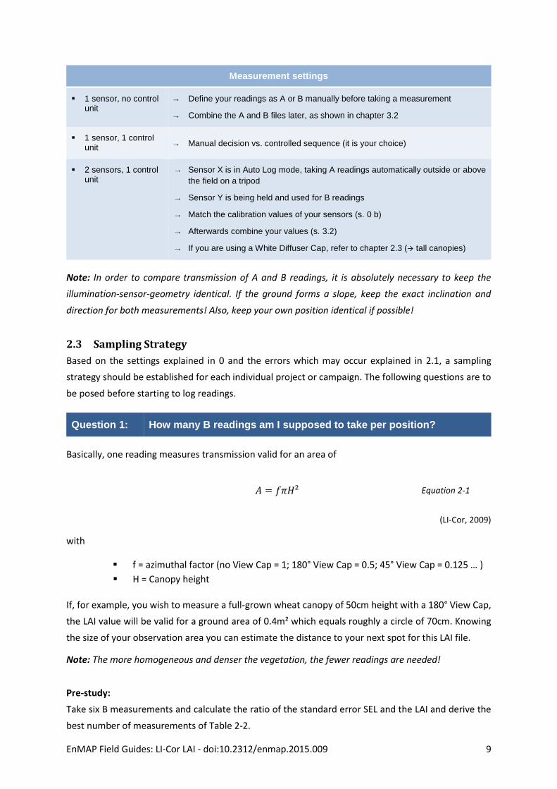
Measurement settings

1 sensor, no control unit

→ Define your readings as A or B manually before taking a measurement

→ Combine the A and B files later, as shown in chapter 3.2

1 sensor, 1 control unit

→ Manual decision vs. controlled sequence (it is your choice)

2 sensors, 1 control unit

→ Sensor X is in Auto Log mode, taking A readings automatically outside or above

the field on a tripod

→ Sensor Y is being held and used for B readings

→ Match the calibration values of your sensors (s. 0 b)

→ Afterwards combine your values (s. 3.2)

→ If you are using a White Diffuser Cap, refer to chapter 2.3 ( tall canopies)

Note: In order to compare transmission of A and B readings, it is absolutely necessary to keep the

illumination-sensor-geometry identical. If the ground forms a slope, keep the exact inclination and

direction for both measurements! Also, keep your own position identical if possible!

2.3 Sampling Strategy

Based on the settings explained in 0 and the errors which may occur explained in 2.1, a sampling

strategy should be established for each individual project or campaign. The following questions are to

be posed before starting to log readings.

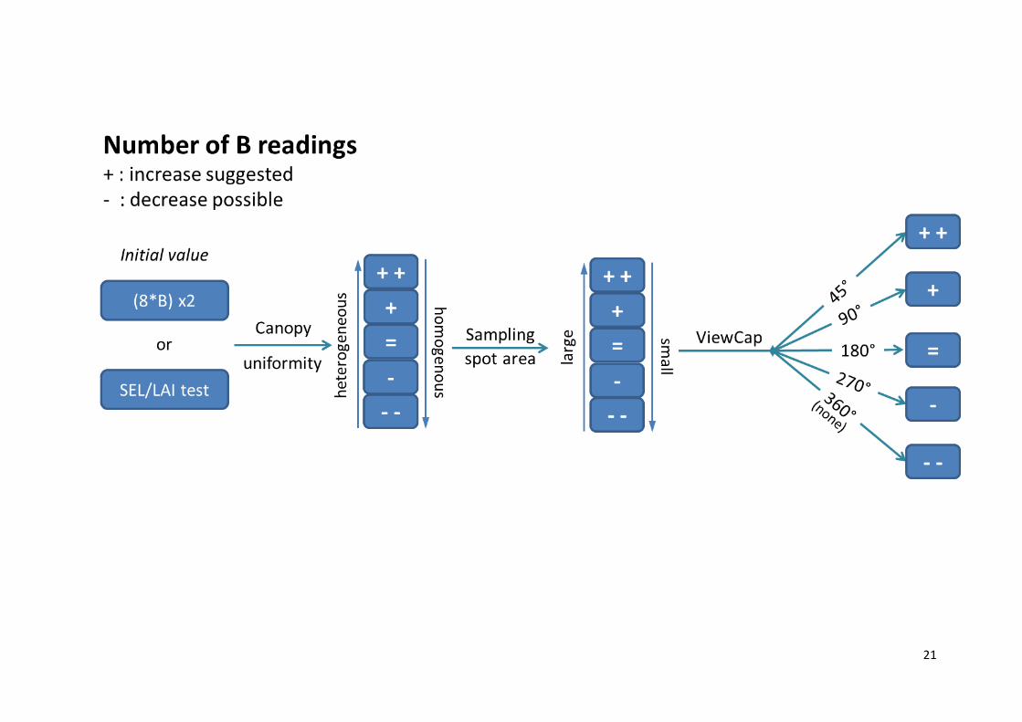
Question 1: How many B readings am I supposed to take per position?

Basically, one reading measures transmission valid for an area of

𝐴 = 𝑓𝜋𝐻² Equation 2-1

(LI-Cor, 2009)

with

f = azimuthal factor (no View Cap = 1; 180° View Cap = 0.5; 45° View Cap = 0.125 … )

H = Canopy height

If, for example, you wish to measure a full-grown wheat canopy of 50cm height with a 180° View Cap,

the LAI value will be valid for a ground area of 0.4m² which equals roughly a circle of 70cm. Knowing

the size of your observation area you can estimate the distance to your next spot for this LAI file.

Note: The more homogeneous and denser the vegetation, the fewer readings are needed!

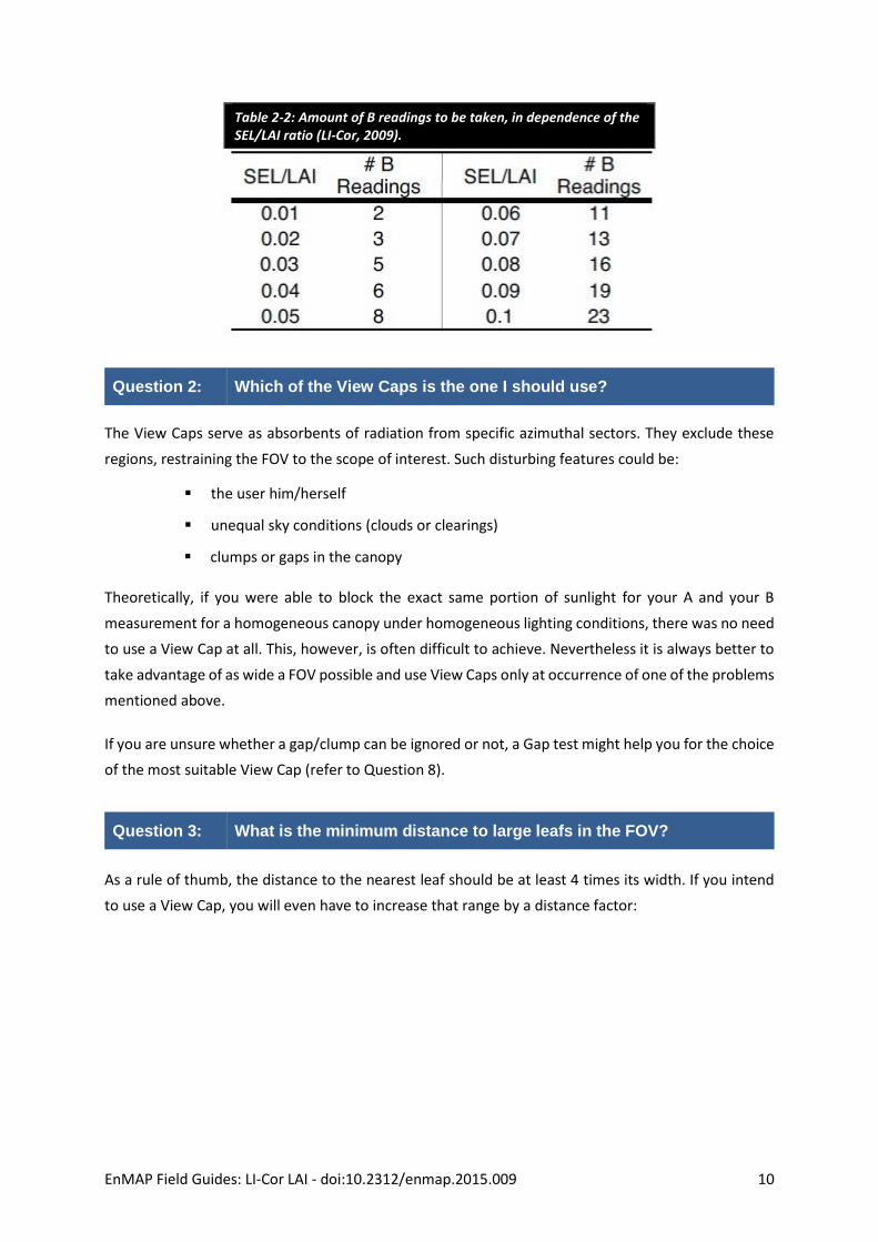
Pre-study:

Take six B measurements and calculate the ratio of the standard error SEL and the LAI and derive the

best number of measurements of Table 2-2.


Table 2-2: Amount of B readings to be taken, in dependence of the SEL/LAI ratio (LI-Cor, 2009).

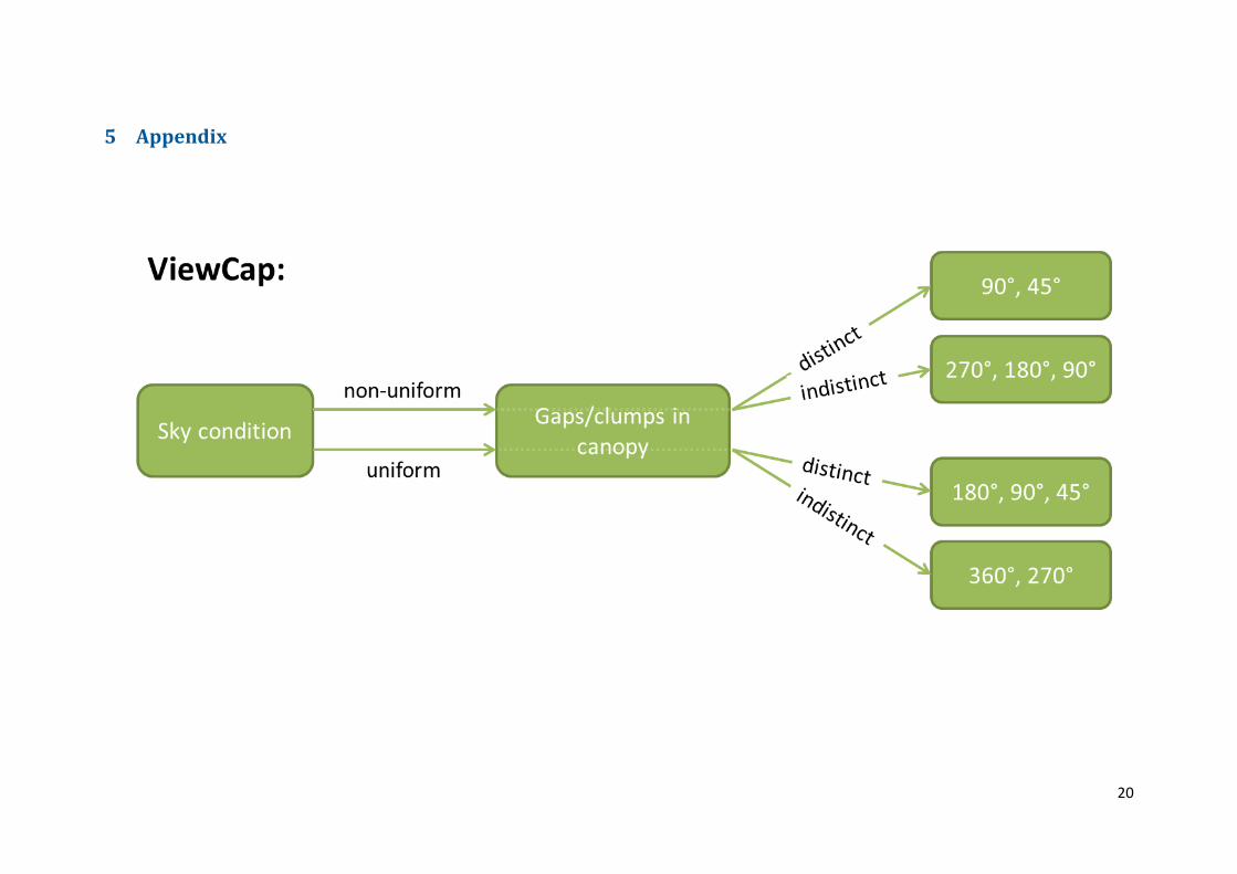
Question 2: Which of the View Caps is the one I should use?

The View Caps serve as absorbents of radiation from specific azimuthal sectors. They exclude these

regions, restraining the FOV to the scope of interest. Such disturbing features could be:

the user him/herself

unequal sky conditions (clouds or clearings)

clumps or gaps in the canopy

Theoretically, if you were able to block the exact same portion of sunlight for your A and your B

measurement for a homogeneous canopy under homogeneous lighting conditions, there was no need

to use a View Cap at all. This, however, is often difficult to achieve. Nevertheless it is always better to

take advantage of as wide a FOV possible and use View Caps only at occurrence of one of the problems

mentioned above.

If you are unsure whether a gap/clump can be ignored or not, a Gap test might help you for the choice

of the most suitable View Cap (refer to Question 8).

Question 3: What is the minimum distance to large leafs in the FOV?

As a rule of thumb, the distance to the nearest leaf should be at least 4 times its width. If you intend

to use a View Cap, you will even have to increase that range by a distance factor:


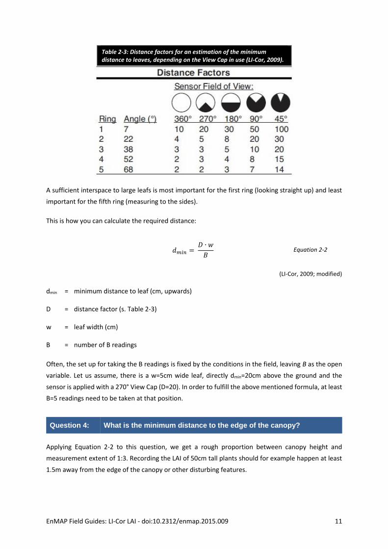
Table 2-3: Distance factors for an estimation of the minimum distance to leaves, depending on the View Cap in use (LI-Cor, 2009).

A sufficient interspace to large leafs is most important for the first ring (looking straight up) and least

important for the fifth ring (measuring to the sides).

This is how you can calculate the required distance:

𝑑𝑚𝑖𝑛 = 𝐷 ∙ 𝑤

𝐵 Equation 2-2

(LI-Cor, 2009; modified)

dmin = minimum distance to leaf (cm, upwards)

D = distance factor (s. Table 2-3)

w = leaf width (cm)

B = number of B readings

Often, the set up for taking the B readings is fixed by the conditions in the field, leaving B as the open

variable. Let us assume, there is a w=5cm wide leaf, directly dmin=20cm above the ground and the

sensor is applied with a 270° View Cap (D=20). In order to fulfill the above mentioned formula, at least

B=5 readings need to be taken at that position.

Question 4: What is the minimum distance to the edge of the canopy?

Applying Equation 2-2 to this question, we get a rough proportion between canopy height and

measurement extent of 1:3. Recording the LAI of 50cm tall plants should for example happen at least

1.5m away from the edge of the canopy or other disturbing features.


Question 5: What do I do if measurements at complete sun exposure are inevitable and I do not own a LAI2200C or 2200CLEAR Kit?

There is a general underestimation of the LAI when the fisheye lens is exposed to the sun or faces sunlit

leaves in the FOV. If the canopy is dense and homogeneous, you will not face big problems for your B

readings. Concerning sparse or inhomogeneous canopies with no possibility to shade the lens, here is

one way how to deal with this impractical situation:

Deriving a Sun-factor to deal with direct sunlight

(1) Go out to the field and take all required measurements for all of your transects or spots

(2) When sun is low and there is only diffuse sunlight left, revisit your site and repeat the measurements of one representative ‘average’ transect or spot

(3) Compare the two datasets and calculate a Sun-factor which you later apply to the original data, e.g. with

the software FV2200.

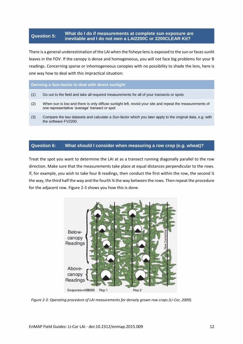
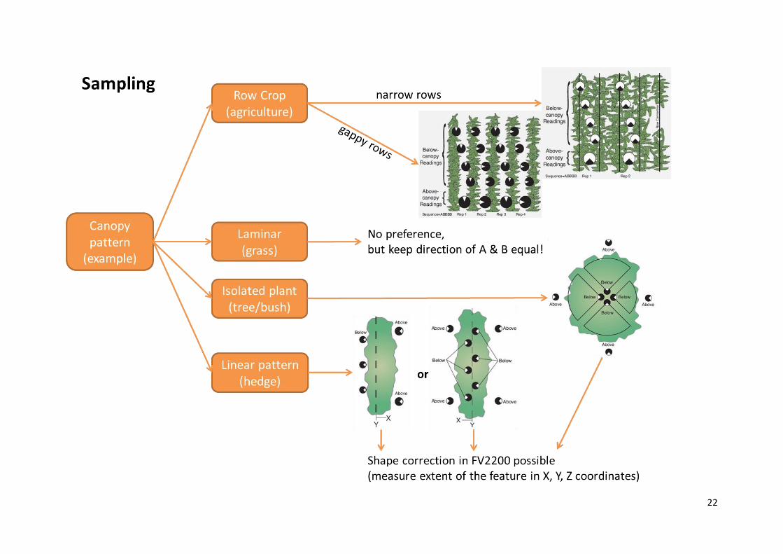
Question 6: What should I consider when measuring a row crop (e.g. wheat)?

Treat the spot you want to determine the LAI at as a transect running diagonally parallel to the row

direction. Make sure that the measurements take place at equal distances perpendicular to the rows.

If, for example, you wish to take four B readings, then conduct the first within the row, the second ¼

the way, the third half the way and the fourth ¾ the way between the rows. Then repeat the procedure

for the adjacent row. Figure 2-3 shows you how this is done.

Figure 2-3: Operating procedure of LAI measurements for densely grown row crops (LI-Cor, 2009).


If gaps between rows are relatively small, you can use wide View Caps. If they are considerably large,

take the 45° View Cap and take one series parallel to the row direction and one in 90° angle to the first

one (s. Figure 2-4). After all: the larger the gaps, the more repetitions are recommended.

Figure 2-4: Operating procedure of LAI measurements for sparsely grown row crops (LI-Cor, 2009).

Question 7: What should I consider when measuring tall canopies (e.g. maize)?

The major difficulty of measuring tall canopies is to get proper A readings. If it is possible to keep the

sensor horizontal and lighting conditions stay diffuse (dawn, homogeneous cloud cover, …) the sensor

can be held above the user’s head to stand out of the canopy. Problems occur, however, when plants

have grown too tall or when shading the lens is necessary to avoid direct sunlight. Mainly, there are

two ways to deal with this complicacy:

Two-Sensor mode

One sensor arm is detached from the console to operate in autonomous mode. It is placed aside the

canopy in exactly the same orientation as the second sensor arm connected to the console in attached

mode. Set the first sensor to Auto Log mode and let it record A readings in determined intervals while

taking B readings with the other sensor. Later, the two data sources need to be merged and LAI files

recomputed (s. 3.2).

LAI2200C or 2200CLEAR Kit: If you have a White Diffuser Cap available, the autonomously measuring

sensor needs to take K records for scattering corrections from time to time (s. 2.2.4). For the FV2200

software to distinguish between real A readings and a 3A or 4A sequence, the latters are ‘disguised’ as


B readings and are therefore called 2BA or 3BA respectively. Proceed as follows (intervals need to be

set at least to 30 seconds):

Measuring tall canopies with two sensors

(1) Wait for an Auto Log

(2) Press the A/B button to change to B readings

(3) Exchange the currently used View Cap with the White Diffuser Cap

(4) Let the sun shine directly onto the sensor and hit LOG (1st B)

(5) Shade the sun and hit LOG again (2nd B)

(6) If you wish to simulate a 4A-sequence (heterogeneous sky conditions): put on the 270° View Cap or shade the sensor with as little shadow as possible and hit LOG (3rd B)

(7) Reassemble the original View Cap and press A/B to switch to A readings again (blue LED). The next automatically taken A measurement will finish the BB(B)A sequence.

Note: It is important to stick to one way of collecting readings for K records. Either you go for 3A/4A or

for 2BA/3BA. 3A or 4A sequences need to be surrounded by B readings. 2BA/3BA readings need to be

surrounded by A readings!

One-sensor mode

When using only one sensor, you may wish to take an A reading at a suitable spot and then plunge into

the tall canopy for a larger number of B readings. Since lighting conditions change during that time

period, the LAI needs to be computed based on reliable reference data of the current irradiation. To

achieve this, set Transcomp – Determine Above to Interpolate. Take an A reading at the beginning,

preferably outside the canopy. Take a set of B readings and finish it with another A reading at the end

of your transect. The console will then chronologically linearly interpolate between both reference

measurements and assign these values to the B records.

Question 8: How do I have to deal with large gaps?

High transmission values in gaps will generally decrease the LAI due to the mathematical computation

method of that parameter (i.e. averaging a logarithm). Therefore, individual low LAI measurements

will depress the overall index excessively. Intentional avoidance of gappy spots on the other hand equal

a subjective selection which leads to an incorrect representation of that place. When a gap is

unavoidably part of the sampling transect, make sure to use a narrow View Cap to decrease the weight

of low LAI values, but measure it nonetheless.

Other than that you can skirt around this error source by computing the effective LAIs (LAIeff) which is

the product of the measured LAIs and the inherent Apparent Clumping Factor ACF. LAIeff can only be

compared with other LAIeff values though.


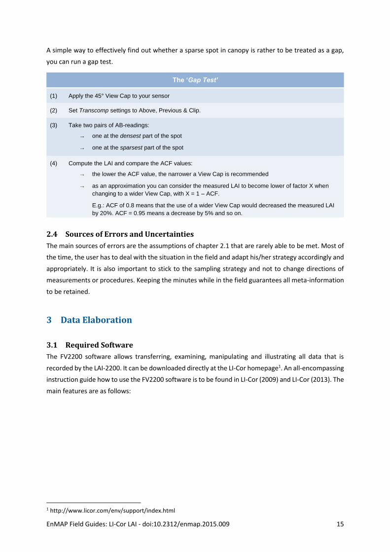
A simple way to effectively find out whether a sparse spot in canopy is rather to be treated as a gap,

you can run a gap test.

The ‘Gap Test’

(1) Apply the 45° View Cap to your sensor

(2) Set Transcomp settings to Above, Previous & Clip.

(3) Take two pairs of AB-readings:

→ one at the densest part of the spot

→ one at the sparsest part of the spot

(4) Compute the LAI and compare the ACF values:

→ the lower the ACF value, the narrower a View Cap is recommended

→ as an approximation you can consider the measured LAI to become lower of factor X when

changing to a wider View Cap, with X = 1 – ACF.

E.g.: ACF of 0.8 means that the use of a wider View Cap would decreased the measured LAI

by 20%. ACF = 0.95 means a decrease by 5% and so on.

2.4 Sources of Errors and Uncertainties

The main sources of errors are the assumptions of chapter 2.1 that are rarely able to be met. Most of

the time, the user has to deal with the situation in the field and adapt his/her strategy accordingly and

appropriately. It is also important to stick to the sampling strategy and not to change directions of

measurements or procedures. Keeping the minutes while in the field guarantees all meta-information

to be retained.

3 Data Elaboration

3.1 Required Software

The FV2200 software allows transferring, examining, manipulating and illustrating all data that is

recorded by the LAI-2200. It can be downloaded directly at the LI-Cor homepage1. An all-encompassing

instruction guide how to use the FV2200 software is to be found in LI-Cor (2009) and LI-Cor (2013). The

main features are as follows:

1 http://www.licor.com/env/support/index.html


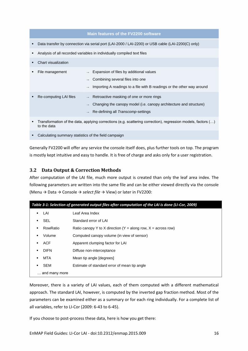
Main features of the FV2200 software

Data transfer by connection via serial port (LAI-2000 / LAI-2200) or USB cable (LAI-2200(C) only)

Analysis of all recorded variables in individually compiled text files

Chart visualization

File management → Expansion of files by additional values

→ Combining several files into one

→ Importing A readings to a file with B readings or the other way around

Re-computing LAI files → Retroactive masking of one or more rings

→ Changing the canopy model (i.e. canopy architecture and structure)

→ Re-defining all Transcomp-settings

Transformation of the data, applying corrections (e,g. scattering correction), regression models, factors (…) to the data

Calculating summary statistics of the field campaign

Generally FV2200 will offer any service the console itself does, plus further tools on top. The program

is mostly kept intuitive and easy to handle. It is free of charge and asks only for a user registration.

3.2 Data Output & Correction Methods

After computation of the LAI file, much more output is created than only the leaf area index. The

following parameters are written into the same file and can be either viewed directly via the console

(Menu Data Console select file View) or later in FV2200:

Table 3-1: Selection of generated output files after computation of the LAI is done (LI-Cor, 2009)

LAI Leaf Area Index

SEL Standard error of LAI

RowRatio Ratio canopy Y to X direction (Y = along row, X = across row)

Volume Computed canopy volume (in view of sensor)

ACF Apparent clumping factor for LAI

DIFN Diffuse non-interceptance

MTA Mean tip angle [degrees]

SEM Estimate of standard error of mean tip angle

… and many more

Moreover, there is a variety of LAI values, each of them computed with a different mathematical

approach. The standard LAI, however, is computed by the inverted gap fraction method. Most of the

parameters can be examined either as a summary or for each ring individually. For a complete list of

all variables, refer to LI-Cor (2009: 6-43 to 6-45).

If you choose to post-process these data, here is how you get there:


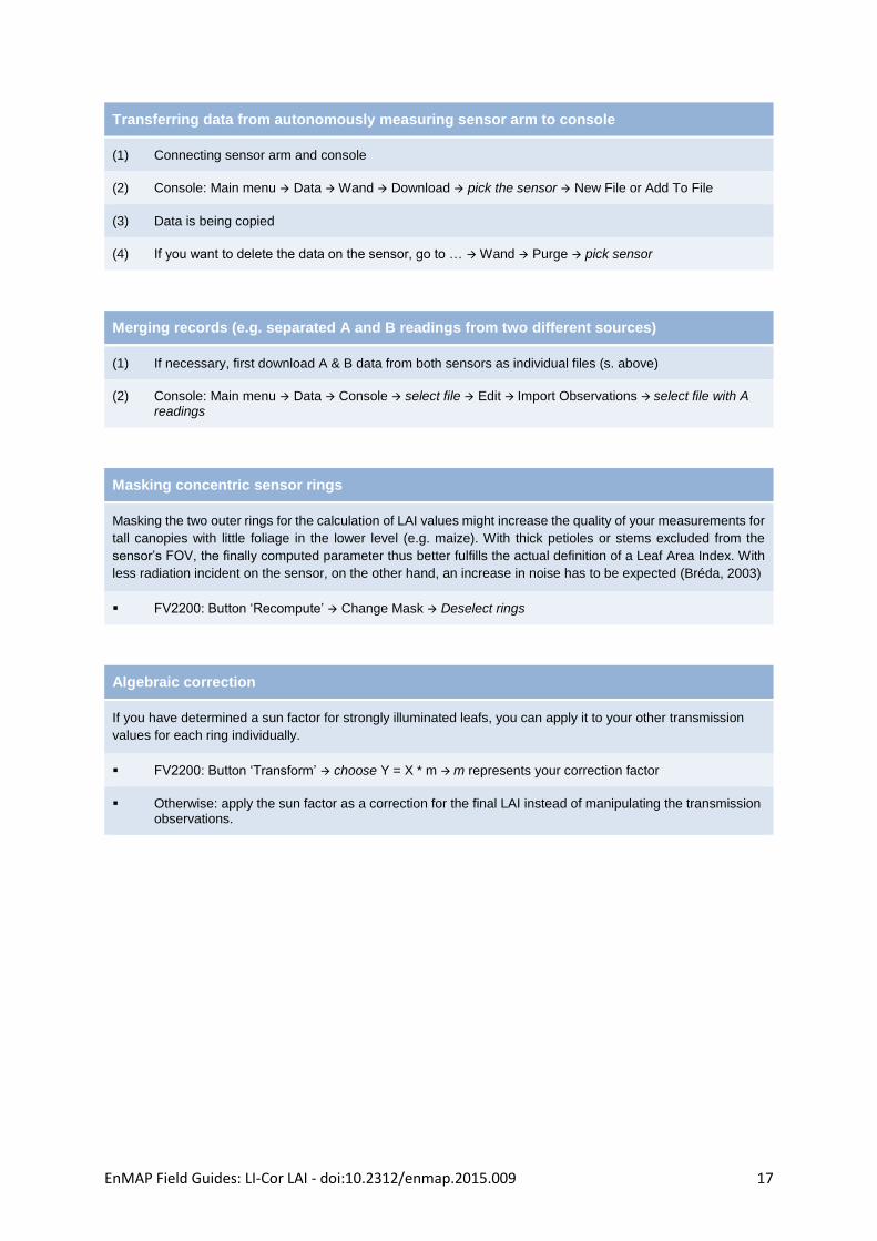
Transferring data from autonomously measuring sensor arm to console

(1) Connecting sensor arm and console

(2) Console: Main menu Data Wand Download pick the sensor New File or Add To File

(3) Data is being copied

(4) If you want to delete the data on the sensor, go to … Wand Purge pick sensor

Merging records (e.g. separated A and B readings from two different sources)

(1) If necessary, first download A & B data from both sensors as individual files (s. above)

(2) Console: Main menu Data Console select file Edit Import Observations select file with A readings

Masking concentric sensor rings

Masking the two outer rings for the calculation of LAI values might increase the quality of your measurements for

tall canopies with little foliage in the lower level (e.g. maize). With thick petioles or stems excluded from the

sensor’s FOV, the finally computed parameter thus better fulfills the actual definition of a Leaf Area Index. With

less radiation incident on the sensor, on the other hand, an increase in noise has to be expected (Bréda, 2003)

FV2200: Button ‘Recompute’ Change Mask Deselect rings

Algebraic correction

If you have determined a sun factor for strongly illuminated leafs, you can apply it to your other transmission

values for each ring individually.

FV2200: Button ‘Transform’ choose Y = X * m m represents your correction factor

Otherwise: apply the sun factor as a correction for the final LAI instead of manipulating the transmission observations.


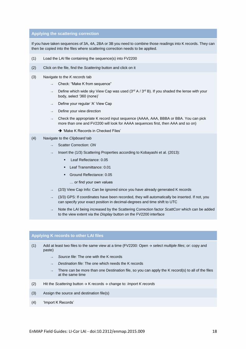
Applying the scattering correction

If you have taken sequences of 3A, 4A, 2BA or 3B you need to combine those readings into K records. They can

then be copied into the files where scattering correction needs to be applied.

(1) Load the LAI file containing the sequence(s) into FV2200

(2) Click on the file, find the Scattering button and click on it

(3) Navigate to the K records tab

→ Check: “Make K from sequence”

→ Define which wide sky View Cap was used (3rd A / 3rd B). If you shaded the lense with your

body, select ‘360 (none)’

→ Define your regular ‘A’ View Cap

→ Define your view direction

→ Check the appropriate K record input sequence (AAAA, AAA, BBBA or BBA. You can pick

more than one and FV2200 will look for AAAA sequences first, then AAA and so on)

‘Make K Records in Checked Files’

(4) Navigate to the Clipboard tab

→ Scatter Correction: ON

→ Insert the (1/3) Scattering Properties according to Kobayashi et al. (2013):

Leaf Reflectance: 0.05

Leaf Transmittance: 0.01

Ground Reflectance: 0.05

… or find your own values

→ (2/3) View Cap Info: Can be ignored since you have already generated K records

→ (3/3) GPS: If coordinates have been recorded, they will automatically be inserted. If not, you

can specify your exact position in decimal-degrees and time shift to UTC

→ Note the LAI being increased by the Scattering Correction factor ScattCorr which can be added

to the view extent via the Display button on the FV2200 interface

Applying K records to other LAI files

(1) Add at least two files to the same view at a time (FV2200: Open select multiple files; or: copy and

paste)

→ Source file: The one with the K records

→ Destination file: The one which needs the K records

→ There can be more than one Destination file, so you can apply the K record(s) to all of the files at the same time

(2) Hit the Scattering button K records change to: Import K records

(3) Assign the source and destination file(s)

(4) ‘Import K Records’


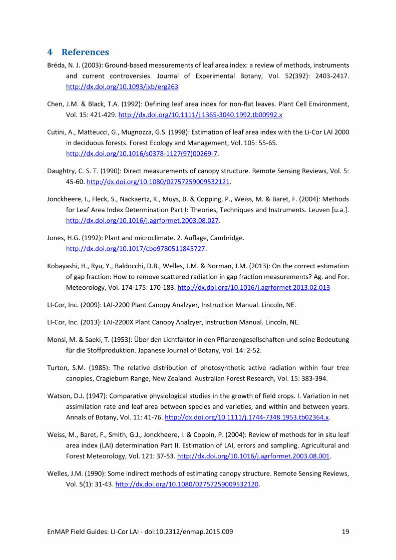
4 References

Bréda, N. J. (2003): Ground-based measurements of leaf area index: a review of methods, instruments

and current controversies. Journal of Experimental Botany, Vol. 52(392): 2403-2417.

http://dx.doi.org/10.1093/jxb/erg263

Chen, J.M. & Black, T.A. (1992): Defining leaf area index for non-flat leaves. Plant Cell Environment,

Vol. 15: 421-429. http://dx.doi.org/10.1111/j.1365-3040.1992.tb00992.x

Cutini, A., Matteucci, G., Mugnozza, G.S. (1998): Estimation of leaf area index with the Li-Cor LAI 2000

in deciduous forests. Forest Ecology and Management, Vol. 105: 55-65.

http://dx.doi.org/10.1016/s0378-1127(97)00269-7.

Daughtry, C. S. T. (1990): Direct measurements of canopy structure. Remote Sensing Reviews, Vol. 5:

45-60. http://dx.doi.org/10.1080/02757259009532121.

Jonckheere, I., Fleck, S., Nackaertz, K., Muys, B. & Copping, P., Weiss, M. & Baret, F. (2004): Methods

for Leaf Area Index Determination Part I: Theories, Techniques and Instruments. Leuven [u.a.].

http://dx.doi.org/10.1016/j.agrformet.2003.08.027.

Jones, H.G. (1992): Plant and microclimate. 2. Auflage, Cambridge.

http://dx.doi.org/10.1017/cbo9780511845727.

Kobayashi, H., Ryu, Y., Baldocchi, D.B., Welles, J.M. & Norman, J.M. (2013): On the correct estimation

of gap fraction: How to remove scattered radiation in gap fraction measurements? Ag. and For.

Meteorology, Vol. 174-175: 170-183. http://dx.doi.org/10.1016/j.agrformet.2013.02.013

LI-Cor, Inc. (2009): LAI-2200 Plant Canopy Analzyer, Instruction Manual. Lincoln, NE.

LI-Cor, Inc. (2013): LAI-2200X Plant Canopy Analzyer, Instruction Manual. Lincoln, NE.

Monsi, M. & Saeki, T. (1953): Über den Lichtfaktor in den Pflanzengesellschaften und seine Bedeutung

für die Stoffproduktion. Japanese Journal of Botany, Vol. 14: 2-52.

Turton, S.M. (1985): The relative distribution of photosynthetic active radiation within four tree

canopies, Cragieburn Range, New Zealand. Australian Forest Research, Vol. 15: 383-394.

Watson, D.J. (1947): Comparative physiological studies in the growth of field crops. I. Variation in net

assimilation rate and leaf area between species and varieties, and within and between years.

Annals of Botany, Vol. 11: 41-76. http://dx.doi.org/10.1111/j.1744-7348.1953.tb02364.x.

Weiss, M., Baret, F., Smith, G.J., Jonckheere, I. & Coppin, P. (2004): Review of methods for in situ leaf

area index (LAI) determination Part II. Estimation of LAI, errors and sampling. Agricultural and

Forest Meteorology, Vol. 121: 37-53. http://dx.doi.org/10.1016/j.agrformet.2003.08.001.

Welles, J.M. (1990): Some indirect methods of estimating canopy structure. Remote Sensing Reviews,

Vol. 5(1): 31-43. http://dx.doi.org/10.1080/02757259009532120.

http://dx.doi.org/10.1093/jxb/erg263

http://dx.doi.org/10.1111/j.1365-3040.1992.tb00992.x

http://dx.doi.org/10.1016/s0378-1127(97)00269-7

http://dx.doi.org/10.1080/02757259009532121

http://dx.doi.org/10.1016/j.agrformet.2003.08.027

http://dx.doi.org/10.1017/cbo9780511845727


http://dx.doi.org/10.1111/j.1744-7348.1953.tb02364.x


http://dx.doi.org/10.1080/02757259009532120

20

5 Appendix

21

22

23

24

Documents

EnMAP Field Guides - gfz-potsdam.degfzpublic.gfz-potsdam.de/pubman/item/escidoc:1381850/component/... · Instruments for LAI measurements with this method are the SunSCAN of Delta-T