Automatica 42 (2006) 1011–1016www.elsevier.com/locate/automatica

Brief paper

Enlarging the terminal region of nonlinear model predictive controlusing the support vector machine method�

C.J. Onga,∗, D. Suia, E.G. Gilbertb

aDepartment of Mechanical Engineering, Singapore-MIT Alliance, National University of Singapore, SingaporebDepartment of Aerospace Engineering, University of Michigan, Ann Arbor, MI, USA

Received 16 September 2004; received in revised form 16 January 2006; accepted 8 February 2006

Abstract

In this paper, receding horizon model predictive control (RHMPC) of nonlinear systems subject to input and state constraints is considered.We propose to estimate the terminal region and the terminal cost off-line using support vector machine learning. The proposed approachexploits the freedom in the choices of the terminal region and terminal cost needed for asymptotic stability. The resulting terminal regions arelarge and, hence provide for large domains of attraction of the RHMPC. The promise of the method is demonstrated with two examples.� 2006 Elsevier Ltd. All rights reserved.

Keywords: Nonlinear model predictive control; Support vector machine; Constraints; Stability; Terminal conditions

1. Introduction

We consider the receding horizon model predictive control(RHMPC) approach for a nonlinear discrete-time constraineddynamic system:

x(t + 1) = f (x(t), u(t)), u(t) ∈ U, x(t) ∈ X ∀t �0,

(1)

where x(t) and u(t) are the state and control variables and X ⊂Rn and U ⊂ Rm are the corresponding constraint sets. Manyapproaches to RHMPC for such a system have been proposed(see for example, Allgöwer & Zheng, 2000; Mayne, Rawlings,Rao, & Scokaert, 2000; and others). Set-theoretic approaches(Chen & Allgöwer, 1998; Magni, Nicolao, Magnani, &Scattolini, 2001; Mayne & Michalska, 1990; Michalska &Mayne, 1993 and others) use a terminal constraint set Xf and a

� This paper was not presented at any IFAC meeting. This paper wasrecommended for publication in revised form by Associate Editor MartinGuay under the direction of Editor Frank Allgower.

∗ Corresponding author.E-mail addresses: mpeongcj@nus.edu.sg (C.J. Ong),

suidan@nus.edu.sg (D. Sui), elmerg@umich.edu (E.G. Gilbert).

0005-1098/$ - see front matter � 2006 Elsevier Ltd. All rights reserved.doi:10.1016/j.automatica.2006.02.023

terminal cost F to increase the domain of attraction and mini-mize online computational effort. These methods typically relyon properties of the linearized system for the characterizationsof Xf and F and prove, under reasonable assumptions, theasymptotic stability of the origin under RHMPC. With limitedassumptions on the properties of f, the domains of attractionfor such methods are naturally small. Unlike the set-theoreticapproach, this paper shows the use of approximating functionsin RHMPC by characterizing Xf and F using support vectormachine (SVM) learning. The resulting Xf and hence the do-mains of attraction are much larger. When X is compact, thisapproach also results in lower online computational effort asshorter horizons can be used. The use of approximating func-tion in model predictive control (MPC) is not new. Parisini andZoppoli (1995) apply neural networks to directly approximatethe closed-loop MPC control law, without the use of Xf andF. Such an approach requires accurate approximation to ensureclosed-loop stability. Our approach exploits the flexibility in thechoices of Xf and F and is less demanding in terms of the ap-proximating accuracy. We demonstrate the effectiveness of theapproach on two low-dimensional systems (n�4). For higher-dimensional systems, the online computations are expected toincrease reasonably although the off-line computations becomeincreasingly demanding with n.

1012 C.J. Ong et al. / Automatica 42 (2006) 1011–1016

Standard notation is adopted: int(D) is the interior of D ⊂Rn, x · y is the inner product of x, y ∈ Rn, ‖x‖2 = x · x and‖(x, u)‖ is the norm on the combined vector [xTuT] ∈ Rn+m

for x ∈ Rn, u ∈ Rm.

2. Preliminaries

The RHMPC of (1) is based on the solution, at each time t,of the following finite horizon (FH) optimal control problemover u = {u(0|t), u(1|t), . . . , u(N − 1|t)}

min J (x, u) =N−1∑i=0

�(x(i|t), u(i|t)) + F(x(N |t)) (2)

s.t. x(i + 1|t) = f (x(i|t), u(i|t)), i = 0, . . . , N − 1, (3)

x(0|t) = x(t) := x, (4)

u(i|t) ∈ U, x(i|t) ∈ X, i = 0, . . . , N − 1, (5)

x(N |t) ∈ Xf , (6)

where � is the stage cost, Xf is the terminal set and F is theterminal cost. Let XN := {x : (3)–(6) are satisfied.}, the set ofstates steerable to Xf in N steps or less. Suppose the systemsatisfy the following assumption: (A0) f : Rn × Rm → Rn iscontinuous, f (0, 0) = 0, X ⊂ Rn, U ⊂ Rm are compact andcontain the origin in their respective interiors, � : X × U → R

and F : Xf → R are continuous and non-negative, �(0, 0)=0,FH has a solution for all x ∈ XN .

The use of Xf and F in RHMPC is associated with a localfeedback law u = �f (x) and

x(t + 1) = f (x(t), �f (x(t))), t �0. (7)

Specifically, if �f (x) ∈ U∀x ∈ Xf , f (x, �f (x)) ∈ Xf ∀x ∈Xf , �f (0) = 0 and F is a Lyapunov function on Xf that guar-antees the stability of x(t) = 0 for (7), then the global stabilityof RHMPC is achieved (Mayne et al., 2000). In satisfying theseconditions, there is much freedom in the choices of �f , Xf

and F. For example, it is common (Cannon, Kouvaritakis, &Deshmukh, 2003; Chen, Balance, & O’Reilly, 2001) to chooseu = kx for a fixed k based on various considerations andF(x) = xTPx to be a Lyapunov function related to the lin-earization of (7) at x(t) = 0. Then, Xf is chosen to be

XP = {x : xTPx��}, (8)

where � > 0 is chosen small so that F remains a Lyapunovfunction on all of XP . The resulting smallness of XP impliesa limited size of XN . Consequently, N has to be large so thatXN occupies a good portion of X, a choice that implies higheronline computational cost.

In our approach �f (x) is chosen so that (7) has a stableequilibrium, x(t) = 0, and Xf is its corresponding maximalconstraint-admissible domain of attraction,

Xf := {x(0)|x(t) ∈ X, �f (x(t)) ∈ U, t �0, x(t) → 0}, (9)

and F : Xf → R is the related infinite horizon cost,

F(x) =∞∑t=0

�(x(t), �f (x(t))), ∀x ∈ Xf . (10)

Consider the following assumptions:

(A1) �f : Rn → Rm is continuous and �f (0) = 0.(A2) x = 0 is an exponentially stable equilibrium of (7).(A3) ∃ a c > 0 s.t. �(x, u)�c‖(x, u)‖, ∀x ∈ X, u ∈ U .(A4) ∃ a c > 0 s.t. �(x, u)� c‖(x, u)‖ in a neighborhood of

(x, u) = 0.

The above assumptions are sufficient to ensure stability ofthe RHMPC system. This and other results are stated in the nexttheorem. The proof of them are extensions of the assumptionsof the well-known stability conditions of Mayne et al. (2000)and are hence omitted.

Theorem 2.1. Suppose assumptions (A0)–(A4) are satisfied.Then the following results hold. (i) Xf ⊂ X, 0 ∈ int (Xf ). (ii)�f (x) ∈ U∀x ∈ Xf . (iii) Xf is positively invariant for (7). (iv)F(x) is defined for all x ∈ Xf , F(0) = 0 and F(x) > 0 ∀x ∈Xf \{0} (v) F(f (x, �f (x)) − F(x) = −�(x, �f (x))∀x ∈ Xf .Finally, suppose system (1) is subject to RHMPC with Xf andF defined by (9) and (10), respectively. Then the equilibriumx(t) ≡ 0 is asymptotically stable in the sense that x(t) → 0for all x(0) ∈ XN , i.e., XN is the domain of attraction for theclosed-loop RHMPC system.

Our approach to the characterizations of Xf and F isachieved through SVM learning, motivated by the freedom inthe choices of F and Xf . As defined in (9), Xf is the max-imal constraint-admissible invariant set for a specific �f (x).Other invariant sets of �f (x) exist and are subsets of Xf .There are also many choices of F. Our choice is FR(x), anapproximation to F (x) := (1 + �)F (x) for some � > 0. Letthe error in approximation be ε(x) := F (x) − FR(x) andx+ := f (x, �f (x)). Suppose

0�ε(x)���(x, �f (x)) ∀x ∈ Xf . (11)

Then,

FR(x+) − FR(x) = (1 + �)(F (x+) − F(x)) − ε(x+) + ε(x)

= − (1 + �)�(x, �f (x)) − ε(x+) + ε(x)

� − (1 + �)�(x, �f (x)) + ��(x, �f (x))

= − �(x, �f (x)).

Thus,

FR(x+) − FR(x)� − �(x, �f (x)), ∀x ∈ Xf . (12)

With the above, it is easy (Mayne et al., 2000) to show thefollowing theorem.

Theorem 2.2. Suppose assumptions (A0)–(A4) are satisfied,Xf is replaced by any invariant set that is a subset of Xf andF(x) is replaced by FR(x) in the RHMPC approach with con-dition (11) holding, then the closed-loop RHMPC is asymptot-ically stable in the sense as defined in Theorem 2.1.

C.J. Ong et al. / Automatica 42 (2006) 1011–1016 1013

3. Characterization of Xf

Our characterization of Xf follows the approach describedin Ong, Keerthi, Gilbert, and Zhang (2004). It considers system(7) with �f (x)=Kx where K is determined from some system-atic procedure. The characterization of Xf takes the form of ascalar function, O(x) such that Xf := {x : O(x)�0} closelyapproximates Xf . To do so, (7) is solved numerically for manyinitial points x(0) = xi ∈ X and for each xi , the condition ofxi ∈ Xf is determined. Two point sets, one containing pointsin Xf and the other containing points in X\Xf , are collected.These sets form the training data in a two-class support vectorclassification (SVC) problem. The resulting decision functionis O(x). Like most SVC applications, many points are collectedfor the training process but O(x) is defined by a small portion(10–20%) of these points. Obviously, if the training data arepoorly chosen, it is not reasonable to expect Xf to be closeto Xf . A careful collection of these training points is madepossible by (i) knowing the characterization of the boundaryof Xf using a modified theory based on Praprost and Loparo(1996) and (ii) an adaptive procedure for iteratively selectingnew points for training the SVC to improve accuracy and effi-ciency.

For every xi ∈ Xf (xi ∈ X\Xf ), an additional variable yi =+1 (yi =−1) is introduced. Let I+={i : yi =+1} and I−={i :yi=−1}. Our formulation of SVC finds a separating hyperplanein a high (possible infinite) dimensional Hilbert space H in theform of O(x) := w · �(x) + b = 0 with w ∈ H and b ∈ R bysolving the following problem:

minw,b,�

1

2w · w + C

∑i

�i (13)

s.t. w · �(xi) + b�1 − �i ∀i ∈ I+, (14)

w · �(xi) + b� − 1 ∀i ∈ I−, �i �0. (15)

Here function � : Rn → H maps x into H, �i is a slackvariable and C is a trade-off parameter. The choices of � andC are discussed later. Unlike standard formulation, the aboverestricts the use of �i to points in Xf only and not for xi ∈X\Xf . Hence, it allows O(x) to classify safe points as unsafebut not the other way. The optimization problem (13)–(15) isconvex and is typically solved via its dual formulation. Let� be the Lagrange multiplier vector for the first two sets ofconstraints in (14) and (15). Its Wolfe dual (Fletcher, 1987) is

min�

1

2

∑i

∑j

�i�j yiyj�(xi) · �(xj ) −∑

i

�i (16)

s.t.∑

�iyi = 0, (17)

C��i �0∀i ∈ I+, �i �0 ∀i ∈ I−. (18)

The solution of (16)–(18) can be found by modifying standardsolvers of SVC.

When the SVM learning process is completed, the functionO(x) is given by O(x)=O(x)−�=∑

i �∗i yi �(xi)·�(x)+b−�

where �∗ is the optimal � for the solution of (16)–(18) and� is a constant determined from validation data (a subset ofthe data not used for training O(x)) so as to enforce the strictnegativity of O(x) for unsafe data. It is easy to see that O(x)

is determined by the non-zero �∗i , each corresponds to one xi

known as a support vector. As the set of support vectors is asmall fraction of the training data, online computation of O(x)

can be quite efficient.The inner product �(x) · �(xi) can be evaluated easily de-

pending on the choice of the kernel function �. Various kernelfunctions are available and a common choice is the Gaussiankernel:

�(x) · �(xi) = ‖x − xi‖2

2�2

for some � > 0. The values of � and C affect the approximatingcapability of SVC and their correct values can be determinedfrom the cross-validation process (Scholköpf & Smola, 2002;Vapnik, 1995).

4. Characterization of F

Like SVC, support vector regression (SVR) (Scholköpf& Smola, 2002; Shevade, Keerthi, Bhattacharyya & Murthy,2000) finds a regression function FR : Xf → R thatapproximates F represented by a group of points yi :=F (xi), i = 1, . . . , m. With (A2), the computation of yi via (10)can be achieved over a finite number of terms if �(x, u) isthe standard linear quadratic (LQ) cost. Let XP of (8) be theLyapunov set of the linearized system and Ni be the shortest tsuch that x(t) ∈ XP for x(0) = xi under (7). The value of yi

from (10) is

yi = (1 + �)

⎛⎝ Ni∑

t=0

�(x(t), Kx(t)) + x(Ni)TPx(Ni)

⎞⎠ . (19)

The SVR formulation differs from the standard as (11) is im-posed exactly, rather than approximately as a penalty term. Itconstructs FR(x) = w · �(x) + b from the data set {xi, yi}m1where w, �(x) ∈ H have the same meanings as in Section 3.The values of w and b are obtained from the following convexoptimization problem:

minw,b

1

2w · w (20)

s.t. 0� yi − w · �(xi) − b�ci, i = 1, . . . , m, (21)

with ci := ��(xi, Kxi). Unlike standard SVR, no slack vari-ables are used for the satisfaction of (21) because of (11). Theoptimization problem is converted to its dual for its numeri-cal solution. Suppose �, � ∈ Rm are the vectors of Lagrangemultipliers of the two sets of inequalities of (21), respectively.

1014 C.J. Ong et al. / Automatica 42 (2006) 1011–1016

Wolfe’s dual (Fletcher, 1987) is:

min�,�

1

2

m∑i

m∑j

(�i − �i )(�j − �j )�(xi)�(xj )

−m∑i

(�i − �i )yi +m∑i

�ici

s.t.m∑i

(�i − �i ) = 0, �i �0, �i �0, i = 1, . . . , m.

Modifications to numerical algorithm for SVR allow the aboveconvex optimization problem to be computed. Suppose �∗

i and�i

∗are the solutions of the dual problem above. The expression

of FR : Xf → R is

FR(x) =m∑i

(�∗i − �i

∗)�(xi) · �(x) + b. (22)

Following (A3), the satisfaction of (11) is easy when ‖x‖ islarge. The accuracy of approximation is only needed when ‖x‖is small. It is therefore important to choose a sufficiently richcollection of xi for the training of FR(x) near the origin. Againthis problem can be simplified if �(x, u) is the standard LQ costand XP ⊂ Xf is the Lyapunov set of (8). In this case, FR canbe chosen as a composite function with FR(x) = (1 + �)xTPx

when x ∈ XP and FR(x) is given by (22) when x ∈ Xf \XP .

5. Enforcing feasibility

While FR(x) can tolerate reasonable inaccuracy to F (x), theapproximation of Xf by Xf introduces a possible difficulty:FH can become infeasible because Xf is not positively invari-ant. When Xf is a reasonable approximation of Xf , such aproblem rarely occurs. To guarantee feasibility, we exploit theavailability of XP (8) for the case where � is the standard LQcost using a modified FH, FHM. FHM optimizes over the sameu space with the following changes: F is replaced with FR in(2), (6) is removed and replaced by the following constraints:

x(i + 1|t) = f (x(i|t), Kx(i|t)), i = N, . . . , N + N , (23)

Kx(i|t) ∈ U, i = N, . . . , N + N , (24)

x(i|t) ∈ Xf , i = N, . . . , N + N − 1, (25)

x(N + N |t) ∈ XP . (26)

Since XP is positively invariant, feasibility of FHM at time t+1follows from the existence of optimal u at time t. The benefit ofa large Xf is realized only if N is sufficiently large. Let T (x) :=min{k : x(k) ∈ XP , x(0) = x, x(i + 1) = f (x(i), Kx(i))}and NT = max{T (x) : x ∈ Xf }. Under (A0) and (A2), NT

is finite. Also, it is easy to see that XN remains unchangedfor any N �NT . Our approach uses a N that is determinedoffline, found during the SVC training process by choosingN := maxi=1,...,mNi where Ni is given by (19). Two results

related to FHM in RHMPC are given. The proof can be foundin the Appendix.

Theorem 5.1. (i) Suppose assumptions (A0)–(A4) aresatisfied,Xf ⊃ XP where XP is an invariant set, N > 0 and FR(x) issuch that (11) holds, then the closed-loop RHMPC using FHMis asymptotically stable in the sense as defined in Theorem 2.1for all x ∈ XN , the state steerable to Xf in N steps of less(ii) Suppose the conditions of (i) hold with N �NT and Xf

approaches Xf in the Hausdorff sense, then XN approachesXN in the Hausdorff sense.

6. Numerical examples

We illustrate our approach with two examples using a P4machine with a 1.8 GHz processor. The nonlinear optimizationroutine used for the solutions of FH and FHM is based on thealgorithm provided for in the Matlab optimization toolbox. Thechoice of � in FR is 0.05.

Example 6.1. (Chen & Allgöwer, 1998) is the discrete-timeimplementation of the continuous-time system x1 =x2 +u(+(1 − )x1), x2 = x1 + u( − 4(1 − )x2) with sampling periodof 0.1 s. The equilibrium point x = 0 is unstable when u = 0and the linearized system is stabilizable for any ∈ (0, 1). Wefollow the settings in Chen and Allgöwer (1998) where U ={u :|u|�2.0}, =0.5, �(x, u)=xTQx +uTRu, Q=0.5I, R =1.0and K = [2.118, 2.118]. In addition, X = {x : ||x||1 �4.0} isadded to denote the region of interest.

To determine O(x), a total of 1047 points are generated butonly 150 are selected, via the adaptive procedure, for training.The overall tuning/training exercise takes 30 s and terminateswith O(x) being determined by 36 support vectors, b=5.6795and � = 0.328. The optimal kernel width is � = 0.3. Similarly,the terminal cost FR is obtained according to the proceduredescribed in Section 4. A total of 2530 points are generated withonly 350 selected for training. The total time needed is 30 min.

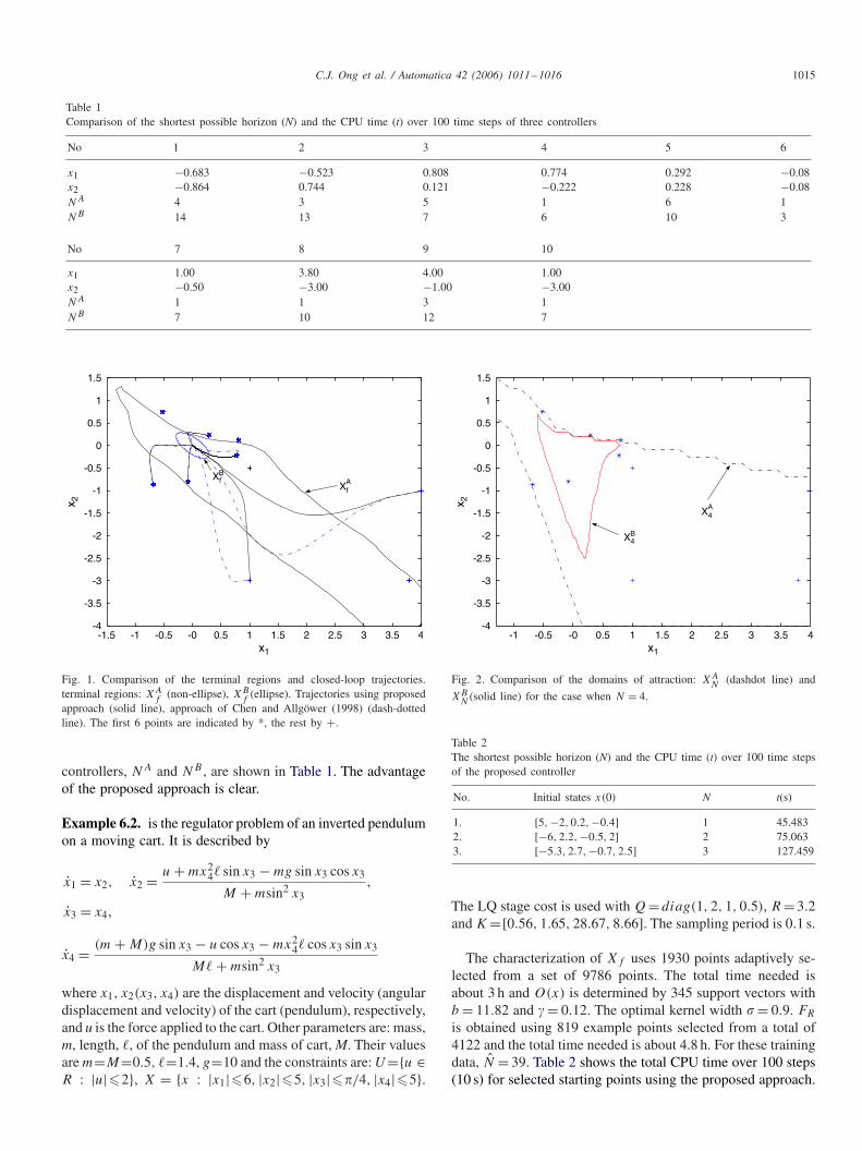
Let superscripts A and B denote, respectively, the results ofour approach with FHM (controller A) and those by the methodof Chen and Allgöwer (1998) (controller B). Fig. 1 shows theterminal regions of the two methods, XA

f = {x : O(x)�0} and

XBf ={x ∈ R2|xTPx�0.7} with P =[16.5911.59; 11.5916.59].

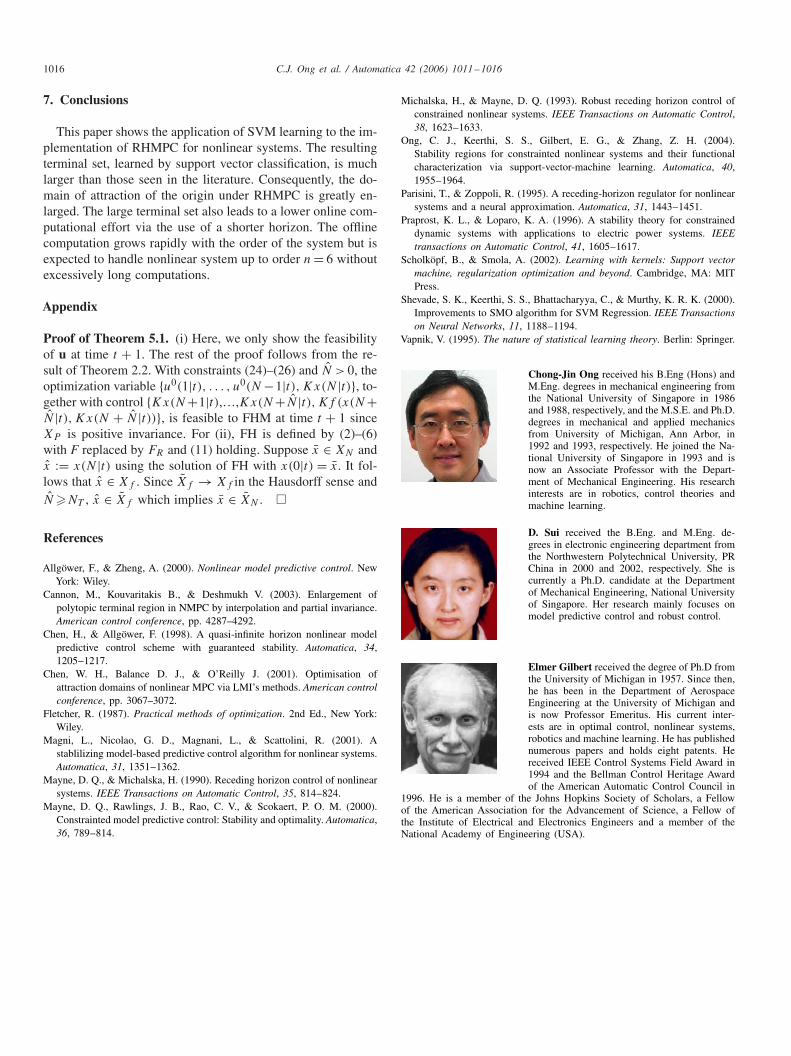
Ten initial points are used in the experiment with the first sixtaken from Chen and Allgöwer (1998) and the rest being new.The locations of these points are indicated in Fig. 1 and Table 1.For each point, 100 steps (10 s) of RHMPC is performed withN =48. To prevent clutter, Fig. 1 shows trajectories of 4 pointsusing both methods. One significant advantage of the large Xf

is the corresponding large domain of attraction, XN (XN inTheorem 5.1). Fig. 2 shows the domains for controllers A, Bwith N = 4 and the set of initial points. All but two points arein XA

4 while only one point is in XB4 . In practice, large Xf

usually means that a short horizon can be used for any givenregion of interest. For an indication of the effect of the sizeof Xf , the respective shortest horizon length needed for both

C.J. Ong et al. / Automatica 42 (2006) 1011–1016 1015

Table 1Comparison of the shortest possible horizon (N) and the CPU time (t) over 100 time steps of three controllers

No 1 2 3 4 5 6

x1 −0.683 −0.523 0.808 0.774 0.292 −0.08x2 −0.864 0.744 0.121 −0.222 0.228 −0.08NA 4 3 5 1 6 1NB 14 13 7 6 10 3

No 7 8 9 10

x1 1.00 3.80 4.00 1.00x2 −0.50 −3.00 −1.00 −3.00NA 1 1 3 1NB 7 10 12 7

-1.5 -1 -0.5 -0 0.5 1 1.5 2 2.5 3 3.5 4-4

-3.5

-3

-2.5

-2

-1.5

-1

-0.5

0

0.5

1

1.5

x1

x 2

XfA

XfB

Fig. 1. Comparison of the terminal regions and closed-loop trajectories.terminal regions: XA

f(non-ellipse), XB

f(ellipse). Trajectories using proposed

approach (solid line), approach of Chen and Allgöwer (1998) (dash-dottedline). The first 6 points are indicated by *, the rest by +.

controllers, NA and NB , are shown in Table 1. The advantageof the proposed approach is clear.

Example 6.2. is the regulator problem of an inverted pendulumon a moving cart. It is described by

x1 = x2, x2 = u + mx24� sin x3 − mg sin x3 cos x3

M + msin2 x3,

x3 = x4,

x4 = (m + M)g sin x3 − u cos x3 − mx24� cos x3 sin x3

M� + msin2 x3

where x1, x2(x3, x4) are the displacement and velocity (angulardisplacement and velocity) of the cart (pendulum), respectively,and u is the force applied to the cart. Other parameters are: mass,m, length, �, of the pendulum and mass of cart, M. Their valuesare m=M=0.5, �=1.4, g=10 and the constraints are: U={u ∈R : |u|�2}, X = {x : |x1|�6, |x2|�5, |x3|�/4, |x4|�5}.

-1 -0.5 -0 0.5 1 1.5 2 2.5 3 3.5 4-4

-3.5

-3

-2.5

-2

-1.5

-1

-0.5

0

0.5

1

1.5

x1

x 2

X4A

X4B

Fig. 2. Comparison of the domains of attraction: XAN

(dashdot line) and

XBN

(solid line) for the case when N = 4.

Table 2The shortest possible horizon (N) and the CPU time (t) over 100 time stepsof the proposed controller

No. Initial states x(0) N t(s)

1. [5, −2, 0.2, −0.4] 1 45.4832. [−6, 2.2, −0.5, 2] 2 75.0633. [−5.3, 2.7, −0.7, 2.5] 3 127.459

The LQ stage cost is used with Q=diag(1, 2, 1, 0.5), R = 3.2and K =[0.56, 1.65, 28.67, 8.66]. The sampling period is 0.1 s.

The characterization of Xf uses 1930 points adaptively se-lected from a set of 9786 points. The total time needed isabout 3 h and O(x) is determined by 345 support vectors withb = 11.82 and � = 0.12. The optimal kernel width � = 0.9. FR

is obtained using 819 example points selected from a total of4122 and the total time needed is about 4.8 h. For these trainingdata, N = 39. Table 2 shows the total CPU time over 100 steps(10 s) for selected starting points using the proposed approach.

1016 C.J. Ong et al. / Automatica 42 (2006) 1011–1016

7. Conclusions

This paper shows the application of SVM learning to the im-plementation of RHMPC for nonlinear systems. The resultingterminal set, learned by support vector classification, is muchlarger than those seen in the literature. Consequently, the do-main of attraction of the origin under RHMPC is greatly en-larged. The large terminal set also leads to a lower online com-putational effort via the use of a shorter horizon. The offlinecomputation grows rapidly with the order of the system but isexpected to handle nonlinear system up to order n = 6 withoutexcessively long computations.

Appendix

Proof of Theorem 5.1. (i) Here, we only show the feasibilityof u at time t + 1. The rest of the proof follows from the re-sult of Theorem 2.2. With constraints (24)–(26) and N > 0, theoptimization variable {u0(1|t), . . . , u0(N −1|t), Kx(N |t)}, to-gether with control {Kx(N +1|t),…,Kx(N +N |t), Kf (x(N +N |t), Kx(N + N |t))}, is feasible to FHM at time t + 1 sinceXP is positive invariance. For (ii), FH is defined by (2)–(6)with F replaced by FR and (11) holding. Suppose x ∈ XN andx := x(N |t) using the solution of FH with x(0|t) = x. It fol-lows that x ∈ Xf . Since Xf → Xf in the Hausdorff sense andN �NT , x ∈ Xf which implies x ∈ XN . �

References

Allgöwer, F., & Zheng, A. (2000). Nonlinear model predictive control. NewYork: Wiley.

Cannon, M., Kouvaritakis B., & Deshmukh V. (2003). Enlargement ofpolytopic terminal region in NMPC by interpolation and partial invariance.American control conference, pp. 4287–4292.

Chen, H., & Allgöwer, F. (1998). A quasi-infinite horizon nonlinear modelpredictive control scheme with guaranteed stability. Automatica, 34,1205–1217.

Chen, W. H., Balance D. J., & O’Reilly J. (2001). Optimisation ofattraction domains of nonlinear MPC via LMI’s methods. American controlconference, pp. 3067–3072.

Fletcher, R. (1987). Practical methods of optimization. 2nd Ed., New York:Wiley.

Magni, L., Nicolao, G. D., Magnani, L., & Scattolini, R. (2001). Astablilizing model-based predictive control algorithm for nonlinear systems.Automatica, 31, 1351–1362.

Mayne, D. Q., & Michalska, H. (1990). Receding horizon control of nonlinearsystems. IEEE Transactions on Automatic Control, 35, 814–824.

Mayne, D. Q., Rawlings, J. B., Rao, C. V., & Scokaert, P. O. M. (2000).Constrainted model predictive control: Stability and optimality. Automatica,36, 789–814.

Michalska, H., & Mayne, D. Q. (1993). Robust receding horizon control ofconstrained nonlinear systems. IEEE Transactions on Automatic Control,38, 1623–1633.

Ong, C. J., Keerthi, S. S., Gilbert, E. G., & Zhang, Z. H. (2004).Stability regions for constrainted nonlinear systems and their functionalcharacterization via support-vector-machine learning. Automatica, 40,1955–1964.

Parisini, T., & Zoppoli, R. (1995). A receding-horizon regulator for nonlinearsystems and a neural approximation. Automatica, 31, 1443–1451.

Praprost, K. L., & Loparo, K. A. (1996). A stability theory for constraineddynamic systems with applications to electric power systems. IEEEtransactions on Automatic Control, 41, 1605–1617.

Scholköpf, B., & Smola, A. (2002). Learning with kernels: Support vectormachine, regularization optimization and beyond. Cambridge, MA: MITPress.

Shevade, S. K., Keerthi, S. S., Bhattacharyya, C., & Murthy, K. R. K. (2000).Improvements to SMO algorithm for SVM Regression. IEEE Transactionson Neural Networks, 11, 1188–1194.

Vapnik, V. (1995). The nature of statistical learning theory. Berlin: Springer.

Chong-Jin Ong received his B.Eng (Hons) andM.Eng. degrees in mechanical engineering fromthe National University of Singapore in 1986and 1988, respectively, and the M.S.E. and Ph.D.degrees in mechanical and applied mechanicsfrom University of Michigan, Ann Arbor, in1992 and 1993, respectively. He joined the Na-tional University of Singapore in 1993 and isnow an Associate Professor with the Depart-ment of Mechanical Engineering. His researchinterests are in robotics, control theories andmachine learning.

D. Sui received the B.Eng. and M.Eng. de-grees in electronic engineering department fromthe Northwestern Polytechnical University, PRChina in 2000 and 2002, respectively. She iscurrently a Ph.D. candidate at the Departmentof Mechanical Engineering, National Universityof Singapore. Her research mainly focuses onmodel predictive control and robust control.

Elmer Gilbert received the degree of Ph.D fromthe University of Michigan in 1957. Since then,he has been in the Department of AerospaceEngineering at the University of Michigan andis now Professor Emeritus. His current inter-ests are in optimal control, nonlinear systems,robotics and machine learning. He has publishednumerous papers and holds eight patents. Hereceived IEEE Control Systems Field Award in1994 and the Bellman Control Heritage Awardof the American Automatic Control Council in

1996. He is a member of the Johns Hopkins Society of Scholars, a Fellowof the American Association for the Advancement of Science, a Fellow ofthe Institute of Electrical and Electronics Engineers and a member of theNational Academy of Engineering (USA).