Enhancing Data Processing on Clouds

with Hadoop/HBase

by

Chen Zhang

A thesis

presented to the University of Waterloo

in fulfilment of the

thesis requirement for the degree of

Doctor of Philosophy

in

Computer Science

Waterloo, Ontario, Canada, 2011

c©Chen Zhang 2011

AUTHOR’S DECLARATION

I hereby declare that I am the sole author of this thesis. This is a true copy of the

thesis, including any required final revisions, as accepted by my examiners.

I understand that my thesis may be made electronically available to the public.

Chen Zhang

iii

Abstract

In the current information age, large amounts of data are being generated and

accumulated rapidly in various industrial and scientific domains. This imposes

important demands on data processing capabilities that can extract sensible

and valuable information from the large amount of data in a timely manner.

Hadoop, the open source implementation of Google’s data processing framework

(MapReduce, Google File System and BigTable), is becoming increasingly pop-

ular and being used to solve data processing problems in various application

scenarios. However, being originally designed for handling very large data sets

that can be divided easily in parts to be processed independently with limited

inter-task communication, Hadoop lacks applicability to a wider usage case. As a

result, many projects are under way to enhance Hadoop for different application

needs, such as data warehouse applications, machine learning and data mining

applications, etc. This thesis is one such research effort in this direction. The

goal of the thesis research is to design novel tools and techniques to extend and

enhance the large-scale data processing capability of Hadoop/HBase on clouds,

and to evaluate their effectiveness in performance tests on prototype implementa-

tions. Two main research contributions are described. The first contribution is a

light-weight computational workflow system called "CloudWF" for Hadoop. The

second contribution is a client library called "HBaseSI" supporting transactional

snapshot isolation (SI) in HBase, Hadoop’s database component.

CloudWF addresses the problem of automating the execution of scientific

v

workflows composed of both MapReduce and legacy applications on clouds

with Hadoop/HBase. CloudWF is the first computational workflow system built

directly using Hadoop/HBase. It uses novel methods in handling workflow di-

rected acyclic graph decomposition, storing and querying dependencies in HBase

sparse tables, transparent file staging, and decentralized workflow execution

management relying on the MapReduce framework for task scheduling and fault

tolerance.

HBaseSI addresses the problem of maintaining strong transactional data

consistency in HBase tables. This is the first SI mechanism developed for HBase.

HBaseSI uses novel methods in handling distributed transactional management

autonomously by individual clients. These methods greatly simplify the design

of HBaseSI and can be generalized to other column-oriented stores with similar

architecture as HBase. As a result of the simplicity in design, HBaseSI adds low

overhead to HBase performance and directly inherits many desirable properties

of HBase. HBaseSI is non-intrusive to existing HBase installations and user data,

and is designed to work with a large cloud in terms of data size and the number

of nodes in the cloud.

vi

Acknowledgements

I would like to thank my supervisor, Professor Hans De Sterck, for the inspirational

instructions and guidance as well as the superb diligence, kindness and patience

in his involvement of my PhD research.

I would like to thank my PhD Committee members for giving me valuable

advice and suggestions. Professor Ashraf Aboulnaga’s course on cloud computing

inspired my work on transactional snapshot isolation on HBase. He also provided

great advice on the paper about the Hadoop case study in solving a scientific

computing problem. Professor Kenneth Salem, who is an expert on snapshot

isolation, provided excellent suggestions on my research on the "HBaseSI" project

as well as insightful comments on the "CloudBATCH" project. He also arranged

three public seminars for me to present my work to faculty members and students

in the David R. Cheriton School of Computer Science. Both of them offered

extremely helpful feedback and critique during my proposal defence and arranged

meetings.

I would like to thank the many excellent collaborators and fellow students,

without whom my graduate studies would not have been the same. I also want

to give thanks to the University of Waterloo Faculty of Mathematics, David R.

Cheriton School of Computer Science, SHARCNET and Cybera for providing

generous support for my research work.

Finally, I would like to thank my wife, who has been supporting me whole-

heartedly in numerous ways, for her tolerance and love.

vii

Dedicated to my wife,

Jing Wu,

for her love.

ix

Table of Contents

Author’s Declaration iii

Abstract v

Acknowledgements vii

Dedication ix

Table of Contents xi

List of Tables xv

List of Figures xvii

1 Introduction 1

1.1 Thesis Statement . . . . . . . . . . . . . . . . . . . . . . . . . . . . . . . 3

1.2 Thesis Organization . . . . . . . . . . . . . . . . . . . . . . . . . . . . . 5

1.3 Publications Related to Thesis Work . . . . . . . . . . . . . . . . . . . 6

1.3.1 Main Contributions . . . . . . . . . . . . . . . . . . . . . . . . . 6

1.3.2 Other Contributions . . . . . . . . . . . . . . . . . . . . . . . . 7

2 Background 9

2.1 Grids and Clouds . . . . . . . . . . . . . . . . . . . . . . . . . . . . . . . 9

2.2 Google’s Cloud Software Framework . . . . . . . . . . . . . . . . . . 12

xi

2.3 Hadoop . . . . . . . . . . . . . . . . . . . . . . . . . . . . . . . . . . . . . 13

2.4 HBase . . . . . . . . . . . . . . . . . . . . . . . . . . . . . . . . . . . . . . 14

3 Preliminary and Supportive Work 19

3.1 Research Overview . . . . . . . . . . . . . . . . . . . . . . . . . . . . . . 19

3.2 Preliminary Work . . . . . . . . . . . . . . . . . . . . . . . . . . . . . . . 22

3.2.1 GridBASE . . . . . . . . . . . . . . . . . . . . . . . . . . . . . . . 22

3.2.2 Hadoop Case Studty . . . . . . . . . . . . . . . . . . . . . . . . 25

3.3 Supportive Work . . . . . . . . . . . . . . . . . . . . . . . . . . . . . . . 30

3.3.1 CloudBATCH . . . . . . . . . . . . . . . . . . . . . . . . . . . . . 30

4 CloudWF 37

4.1 Introduction . . . . . . . . . . . . . . . . . . . . . . . . . . . . . . . . . . 38

4.2 CloudWF . . . . . . . . . . . . . . . . . . . . . . . . . . . . . . . . . . . . 43

4.2.1 Expressing Workflows . . . . . . . . . . . . . . . . . . . . . . . 45

4.2.2 Storing Workflows in HBase Tables . . . . . . . . . . . . . . . 48

4.2.3 Staging Files Transparently with HDFS . . . . . . . . . . . . 51

4.2.4 Executing Workflows . . . . . . . . . . . . . . . . . . . . . . . . 53

4.2.5 Optimization: Virtual Start and End Blocks . . . . . . . . . . 54

4.3 Example Scientific Workflow Application Scenario . . . . . . . . . . 55

4.4 Related Work . . . . . . . . . . . . . . . . . . . . . . . . . . . . . . . . . 55

4.4.1 Dataflow and Workflow Systems for Hadoop . . . . . . . . . 56

4.4.2 Legacy Workflow Systems . . . . . . . . . . . . . . . . . . . . . 57

4.4.3 The Pegasus Workflow System . . . . . . . . . . . . . . . . . . 59

4.5 Conclusions and Future Work . . . . . . . . . . . . . . . . . . . . . . . 62

5 Snapshot Isolation for Column Stores on Clouds 65

5.1 Introduction . . . . . . . . . . . . . . . . . . . . . . . . . . . . . . . . . . 65

5.2 Background . . . . . . . . . . . . . . . . . . . . . . . . . . . . . . . . . . 68

5.2.1 Snapshot Isolation . . . . . . . . . . . . . . . . . . . . . . . . . 68

xii

5.2.2 HBase . . . . . . . . . . . . . . . . . . . . . . . . . . . . . . . . . 70

5.3 HBaseSI . . . . . . . . . . . . . . . . . . . . . . . . . . . . . . . . . . . . . 72

5.3.1 System Design . . . . . . . . . . . . . . . . . . . . . . . . . . . . 72

5.3.2 Protocol Walkthrough by Example . . . . . . . . . . . . . . . 82

5.3.3 Read Optimization . . . . . . . . . . . . . . . . . . . . . . . . . 85

5.3.4 Handling Stragglers . . . . . . . . . . . . . . . . . . . . . . . . 88

5.3.5 SI Proof . . . . . . . . . . . . . . . . . . . . . . . . . . . . . . . . 90

5.3.6 Discussion . . . . . . . . . . . . . . . . . . . . . . . . . . . . . . 94

5.4 Performance Evaluation on Amazon EC2 . . . . . . . . . . . . . . . . 98

5.5 Related Work . . . . . . . . . . . . . . . . . . . . . . . . . . . . . . . . . 115

5.6 Conclusions and Future Work . . . . . . . . . . . . . . . . . . . . . . . 118

6 Conclusions and Future Research 121

6.1 Wireless Sensor Networks and Clouds . . . . . . . . . . . . . . . . . . 123

6.2 Mobile Cloud . . . . . . . . . . . . . . . . . . . . . . . . . . . . . . . . . 124

Bibliography 125

xiii

List of Tables

2.1 An example HBase table taken from the HBase website (slightly

modified). A column is specified by the concatenation of a column

family name and a column qualifier. For example, in the first

column, "anchor" is the name of a column family and "cnnsi.com"

is a column qualifier. The symbols "ts8" and "ts9" denote timestamps. 16

5.1 W counter table. W stands for "HBase write timestamp". . . . . . . 73

5.2 R counter table. R stands for "commit request ID". . . . . . . . . . . 73

5.3 C counter table. C stands for "commit timestamp". . . . . . . . . . . 73

5.4 CommitRequestQueue table. . . . . . . . . . . . . . . . . . . . . . . . . 74

5.5 CommitQueue table. . . . . . . . . . . . . . . . . . . . . . . . . . . . . . 75

5.6 Committed table. . . . . . . . . . . . . . . . . . . . . . . . . . . . . . . . 75

5.7 Shop table. . . . . . . . . . . . . . . . . . . . . . . . . . . . . . . . . . . . 83

5.8 Committed table. . . . . . . . . . . . . . . . . . . . . . . . . . . . . . . . 83

5.9 CommitRequestQueue table. . . . . . . . . . . . . . . . . . . . . . . . . 85

5.10 CommitQueue table. . . . . . . . . . . . . . . . . . . . . . . . . . . . . . 85

5.11 Committed table. . . . . . . . . . . . . . . . . . . . . . . . . . . . . . . . 85

5.12 Version table. For example, the most recently read version of

the data item stored in user data location DataLocation1 was

committed by the transaction with commit timestamp C17. . . . . 86

5.13 Committed table. . . . . . . . . . . . . . . . . . . . . . . . . . . . . . . . 90

xv

5.14 Test to show that the Version table is not needed for reading

data items that are written only once. The time recorded in each

column is the time of scanning the table using bare-bones HBase

scan. . . . . . . . . . . . . . . . . . . . . . . . . . . . . . . . . . . . . . . . 105

5.15 Test to show that the Version table is effective to reduce the scan

range in the Committed table. The time recorded in each column

is the total time of running a transaction containing one read

operation using HBaseSI. . . . . . . . . . . . . . . . . . . . . . . . . . 105

xvi

List of Figures

3.1 GridBase design overview. . . . . . . . . . . . . . . . . . . . . . . . . . 23

3.2 Single microscope image with about two dozen cells on a grey

background. Some interior structure can be discerned in every

cell (including the cell membrane, the dark grey cytoplasm, and

the lighter cell nucleus with dark nucleoli inside). Cells that are

close to division appear as bright, nearly circular objects. In a

typical experiment images are captured concurrently for 600 of

these "fields". For each field we acquire about 900 images over a

total duration of 48 hours, resulting in 260 GB of acquired data

per experiment. The data processing task consists of segmenting

each image and tracking all cells individually in time. The cloud

application is designed to handle concurrent processing of many

of these experiments and storing all input and output data in a

structured way. . . . . . . . . . . . . . . . . . . . . . . . . . . . . . . . . 27

3.3 System design overview for the Hadoop case study project. . . . . 28

3.4 SGE Hadoop Integration (taken from online blog post by Oracle). 33

3.5 CloudBATCH architecture overview. . . . . . . . . . . . . . . . . . . . 35

4.1 Breaking up the components of two workflows into independent

blocks and connectors. The HBase tables store the dependencies

between components implicitly. . . . . . . . . . . . . . . . . . . . . . . 42

xvii

4.2 CloudWF system overview. . . . . . . . . . . . . . . . . . . . . . . . . . 44

4.3 First example workflow and XML file (legacy blocks). . . . . . . . . 47

4.4 Second example workflow and XML file (MapReduce blocks). . . . 48

4.5 HBase tables for the example workflow of Figure 2.2. . . . . . . . . 49

4.6 Virtual start and virtual end blocks. . . . . . . . . . . . . . . . . . . . 55

4.7 Pegasus system overview (taken from [38]). . . . . . . . . . . . . . . 60

5.1 Illustration of SI. . . . . . . . . . . . . . . . . . . . . . . . . . . . . . . . 68

5.2 An example SI scenario. . . . . . . . . . . . . . . . . . . . . . . . . . . 70

5.3 Test 1, performance of the timestamp issuing mechanism through

counter tables. . . . . . . . . . . . . . . . . . . . . . . . . . . . . . . . . 100

5.4 Test 2, performance of the start timestamp issuing mechanism. . . 102

5.5 Test 3, comparative performance of executing transactions with SI

against bare-bones HBase without SI. . . . . . . . . . . . . . . . . . . 103

5.6 Test 4, time to traverse a resultset against a varying number of

rows to scan. . . . . . . . . . . . . . . . . . . . . . . . . . . . . . . . . . 105

5.7 Test 5, general performance (total throughput) of executing trans-

actions with SI under different workloads. . . . . . . . . . . . . . . . 107

5.8 Test 5, comparative throughput between SI and estimated success-

ful HBase transactions under the "95/5 mix". . . . . . . . . . . . . . 108

5.9 Test 5, comparative throughput between SI and estimated success-

ful HBase transactions under the "80/20 mix". . . . . . . . . . . . . 108

5.10 Test 5, comparative throughput between SI and estimated success-

ful HBase transactions under "50/50 mix". . . . . . . . . . . . . . . . 109

5.11 Test 5, successful transaction ratio under different types of work-

loads. . . . . . . . . . . . . . . . . . . . . . . . . . . . . . . . . . . . . . . 109

5.12 Test 5, percentage of failing transactions that fail due to the strag-

gler handling mechanism with 0 and 200 milliseconds as timeout

thresholds respectively. . . . . . . . . . . . . . . . . . . . . . . . . . . . 111

xviii

5.13 Test 5, "95/5 mix" wait time in both CommitRequestQueue and

CommitQueue. . . . . . . . . . . . . . . . . . . . . . . . . . . . . . . . . 112

5.14 Test 5, "80/20 mix" wait time in both CommitRequestQueue and

CommitQueue. . . . . . . . . . . . . . . . . . . . . . . . . . . . . . . . . 112

5.15 Test 5, "50/50 mix" wait time in both CommitRequestQueue and

CommitQueue. . . . . . . . . . . . . . . . . . . . . . . . . . . . . . . . . 112

5.16 Test 6, throughput seen at each client under a varying failure ratio.113

5.17 Test 6, average duration of successful transactions under a varying

failure ratio. . . . . . . . . . . . . . . . . . . . . . . . . . . . . . . . . . . 113

5.18 Coefficient of Variance (COV) calculated from data collected in

Test 5. . . . . . . . . . . . . . . . . . . . . . . . . . . . . . . . . . . . . . . 114

5.19 Coefficient of Variance (COV) of Amazon EC2 performance report-

ed in [40]. . . . . . . . . . . . . . . . . . . . . . . . . . . . . . . . . . . 115

xix

Chapter 1

Introduction

Nowadays, large amounts of data are being generated daily from various sources:

web posts on social network sites like Facebook, transactional data at Amazon

and Walmart, data generated by search engines like Google, astronomy and

weather data gathered by NASA, drug testing data at pharmaceutical companies,

etc. These data are also called "Big Data" in some contexts. Big Data are either

structured data that can be stored in relational databases, or unstructured data

that may include audio, video, images, web pages, and many other forms. A

common trait associated with these data is the large scale in terms of data size

and the ever-increasing demand for new techniques to process and make sense

of the data in a timely and scalable1 manner.

The immense data processing scale has posed challenging requirements on

existing distributed programming paradigms and execution environments, and

on the underlying hardware infrastructure, particularly concerning easy pro-

grammability, scalability, fault tolerance and on-demand resource availability.

Under this background, Google was a pioneer in designing a software framework

1In this thesis, two aspects of scalability are of importance: 1. scalability in terms of automati-

cally handling hardware failures that occur with increased frequency for larger systems; and 2.

scalability in terms of performance as problem sizes and cloud sizes increase.

1

[12, 18, 4] for processing large-scale data sets in a scalable and fault tolerant way.

Amazon revolutionarily commercialized an economical way for companies and

the general public to acquire on-demand computing resources through renting

virtual machine instances based on a pay-per-use model [15]. The resources

provided in this way are now referred to as "public clouds". The resources in

traditional clusters and grids belonging to the same organization are referred to

as "private clouds" if the resources are used in similar on-demand and expandable

ways like public clouds. A resource pool consisting of a combination of public

cloud and private cloud resources is called a "hybrid cloud". The term "cloud

computing" is used to refer to this new way of doing computation over cloud

resources.

Hadoop [34], the open source implementation of Google’s system, is a pop-

ular open source cloud computing framework that has shown to perform well

in various usage scenarios (e.g., see [32]). Its MapReduce framework offers

transparent distribution of compute tasks and data with optimized data locality

and task level fault tolerance; its Hadoop Distributed File System (HDFS) offers

a single global interface to access data from anywhere with data replication for

fault tolerance; and its HBase [21] sparse data store allows to manage structured

data on top of HDFS.

Similar to Google’s original system, Hadoop is designed for the processing

of very large data sets that can be divided easily in parts that can be processed

independently with limited inter-task communication over homogeneous com-

puting environment. As Hadoop becomes popular, people find that Hadoop can

also be extended or enhanced to solve a wide spectrum of problems beyond

the original type of computing problems it was designed for. As a result, many

related projects are created to cater to different application needs. For example,

"Hive" [6] is a data warehouse infrastructure that provides data summarization

and ad hoc querying; "Pig" [23] is a high-level dataflow language and execution

2

framework for parallel computation; and "Mahout" [28] is a scalable machine

learning and data mining library, etc.

Among these efforts in enhancing Hadoop, some research problems remain

open for further investigation. For example, there exists no out-of-the-box

support for database transactions involving multiple data rows in HBase sparse

tables; there exist no well-established cloud environment computational workflow

systems on top of Hadoop to easily build and run computational workflows

composed of MapReduce and existing legacy programs; Hadoop is incompatible

with existing cluster batch job queuing systems and lacks support for user access

control, accounting, and legacy batch job processing facilities comparable to

existing cluster job queuing systems, etc.

In this thesis, we focus on research questions pertaining to enhancing software

frameworks for cloud computing. More specifically, we design novel tools and

techniques to extend and enhance the large-scale data processing capability of

Hadoop/HBase on clouds, and to evaluate their effectiveness in performance

tests on prototype implementations.

1.1 Thesis Statement

This thesis addresses the problem of enhancing large-scale data processing on

clouds with Hadoop/HBase in handling computational workflows and maintain-

ing strong transactional data consistency. The two major contributions we report

on in this thesis are as follows.

1. A light-weight computational workflow system, called "CloudWF", is pre-

sented, automating the execution of scientific workflow jobs on clouds

with Hadoop/HBase. CloudWF tackles the problem of easily building and

running computational workflows composed of MapReduce and existing

legacy programs. It is the first workflow management system that is built

3

entirely on top of Hadoop/HBase and targeted to take advantage of the

new Hadoop/HBase architecture for scalability, fault tolerance and ease of

use.

2. A client library, called "HBaseSI", is presented, supporting multi-row dis-

tributed transactions with global strong snapshot isolation (SI) on HBase.

HBaseSI tackles the problem of maintaining strong transactional data con-

sistency in HBase tables under concurrent access in a shared environment.

It is the first snapshot isolation solution for HBase, and it is built entirely

on bare-bones HBase instead of implementing an extra middleware layer

atop.

CloudWF (presented in [46]) is the first workflow management system closely

integrated with Hadoop/HBase that allows the user to build and run compu-

tational workflows composed of both MapReduce and legacy applications on

clouds. The novelties in the design of CloudWF are: 1. A new way to describe

workflow components as self-contained and independent building blocks, separat-

ing executable blocks from connectors; this facilitates easier storage, dependency

handling, file staging, and distribution; 2. A new method to store workflow

component information as well as workflow graph structure (dependencies) in

HBase sparse tables with an efficient way to query and reconstruct dependencies

at run time; 3. A new method to automate file staging between workflow blocks

transparently; 4. A new method to manage multiple workflow instance execu-

tions using a single workflow engine (composed of a set of global HBase tables

and several decentralized distributed system components), while other workflow

systems normally feature one workflow engine process per workflow executed,

which makes load balancing and execution coordination more difficult [39].

HBaseSI is the first distributed transactional system with global SI for HBase.

Our initial version of HBaseSI provided weak SI [48]; the new version presented

in [49] is significantly improved and provides strong SI. Our work on SI for HBase

4

was published independently and at the same time as Google’s Percolator system

for supporting transactions with SI in BigTable. While HBaseSI shares some

important design ideas with Percolator, there are also significant differences (e.g.,

Percolator is intrusive to user data tables, uses data locks and complicated strag-

gler handling mechanisms, may have blocking reads, etc.). Also, Percolator relies

on the "single-row transaction" functionality specific to BigTable, and therefore

cannot be directly implemented on HBase. The major novelties in HBaseSI are: 1.

Non-intrusive to both server configuration and client data - no modifications are

required; 2. A new method in handling distributed transaction commits without

using a central commit engine or traditional distributed coordination methods

such as consensus-based protocols, explicit atomic broadcast, and transactional

data locks. Instead, transactions make commit decisions autonomously; 3. A new

method to guarantee non-blocking start of transactions with fresh and consistent

snapshots as well as strict global commit ordering, relying on a novel distributed

queuing mechanism implemented by standard HBase tables; 4. A new method

to handle straggling and failed transactions without the need for any roll back/-

forward procedures. The approaches followed in HBaseSI can also be applied

to other column-oriented data stores that feature similar data organization as

HBase.

1.2 Thesis Organization

The remaining chapters of the thesis are organized as follows.

Chapter 2 introduces some necessary background information. We will talk

about grids and clouds, key components in Google’s large-scale data processing

framework, Hadoop and HBase.

Chapter 3 describes the preliminary and supportive work I did in the early

stages of my PhD research. This motivates the two main contributions of the

thesis. A brief overview is given of the research projects I have done during my

5

PhD study, showing how they are related as well as their relevance to the main

theme of the thesis. Some details are provided for some of the preliminary and

supportive work.

Chapter 4 describes the CloudWF system for building and running computa-

tional workflows. The design and implementation of the system are described in

detail, and the advantages of the new design over existing systems are discussed.

Chapter 5 describes the HBaseSI system for achieving transactional snapshot

isolation on Hadoop clouds. The detailed system design and implementation

are described as well as a complete protocol walkthrough under an example

application scenario, and performance evaluations using Amazon EC2.

Chapter 6 gives conclusions and describes future research directions.

1.3 Publications Related to Thesis Work

1.3.1 Main Contributions

The publications below are related to the two main contributions of the thesis:

CloudWF and HBaseSI. The conference paper in CloudCom2009 describes the

design and implementation of the CloudWF system (See Chapter 4). The journal

paper describes the significantly improved HBaseSI system with strong SI whereas

the conference paper published in Grid2010 describes the initial HBaseSI system

with weak SI (See Chapter 5).

Journal Publications

1. Chen Zhang and Hans De Sterck. HBaseSI: A Solution for Multi-row

Distributed Transactions with Global Strong Snapshot Isolation on Clouds.

Special Issue: New Directions in Cloud and Grid Computing, Scalable

Computing: Practice and Experience, Vol. 12, No. 2, 2011.

6

Conference Publications

1. CloudCom2009: Chen Zhang and Hans De Sterck. CloudWF: A Computa-

tional Workflow System for Clouds Based on Hadoop. The First Internation-

al Conference on Cloud Computing, Dec 1-4, 2009, Beijing, China. (27%

acceptance)

2. Grid2010: Chen Zhang and Hans De Sterck. Supporting Multi-row Dis-

tributed Transactions with Global Snapshot Isolation Using Bare-bones

HBase. The 11th ACM/IEEE International Conference on Grid Computing,

Oct 25-29, 2010, Brussels, Belgium. (23% acceptance)

1.3.2 Other Contributions

The following publications are related to preliminary and supportive work I have

done during my PhD (See Chapter 3). The journal paper in RNA, the conference

paper in BLSC2007 and the book chapter are results of my involvement in the

research on GridBASE, a light-weight grid computing framework, at the early

stage of my PhD study. At that time, cloud computing was still at its very infancy

while grid computing prevailed. The paper in HPCS2009 describes one of the

first few research attempts at the time it was published to apply Hadoop in

solving scientific computing problems with customized input formats. The paper

published in CloudCom2010 describes supportive work on CloudBATCH, a system

attempting to enable Hadoop with the capability to manage traditional batch job

submissions in clusters.

Journal Publications

1. Ryan Kennedy, Manuel E. Lladser, Zhiyuan Wu, Chen Zhang, Michael Yarus,

Hans De Sterck, and Rob Knight. Natural and Artificial RNAs Occupy the

Same Restricted Region of Sequence Space. RNA, 16:280-289, 2010.

7

Conference and Workshop Publications

1. CloudCom2010: Chen Zhang and Hans De Sterck. CloudBATCH: A Batch

Job Queuing System on Clouds with Hadoop and HBase. The Second IEEE

International Conference on Cloud Computing Technology and Science,

Nov 30 - Dec 3, 2010, Indianapolis, Indiana, USA. (25% acceptance)

2. HPCS2009: Chen Zhang, Ashraf Aboulnaga, Hans De Sterck, Haig Djam-

bazian, and Rob Sladek. Case Study of Scientific Data Processing on a

Cloud Using Hadoop. High Performance Computing Symposium, June

14-17, 2009. Kingston, Ontario, Canada.

3. BLSC2007: Hans De Sterck, Chen Zhang, and Aleks Papo. Database-driven

Grid Computing with GridBASE. The 2007 IEEE International Symposium

on Bioinformatics and Life Science Computing. May 21-23, 2007. Niagara

Falls, Ontario, Canada.

Book Chapter

1. Hans De Sterck, Alex Papo, Chen Zhang, Micah Hamady, and Rob Knight.

Database-driven Grid Computing and Distributed Web Applications: A

Comparison. In "Grids for Bioinformatics and Computational Biology".

Wiley, December 2007. ISBN: 978-0-471-78409-8.

8

Chapter 2

Background

2.1 Grids and Clouds

Grid computing is an abstract concept of orchestrating heterogeneous computing

resources across virtual organizations (VO’s) [17] to solve problems that are

normally computation-intensive and/or data-intensive and cannot be solved

efficiently on a single computer. Grid computing has the objective to provide

an ideal combination of high performance, high reliability and ease of program-

ming. While the grid computing idea was attractive for certain applications and

substantial effort has been dedicated to working out this concept by various

research groups around the world, it has also turned out that the idea was not

easy to realize in practice. Among the stumbling blocks encountered we could

mention security and privacy concerns, lack of hardware or software compati-

bility between heterogeneous computing resources, and the general inertia of

legacy computing environments against change. In fact, the intrinsic difficulties

of optimizing the use of heterogeneous resources and dealing with different

administrative domains within and across VO’s have made it complicated and

difficult to adopt the technology outside of research and educational institutions.

9

Additionally, grids are normally shared by many users at the same time by us-

ing existing queuing systems instead of granting dedicated usage on a per user

basis. This introduces extra complexity in resource discovery, reservation and

monitoring, which further makes the wide adoption of grids difficult. There thus

remained a clear need for transparent, user-friendly and efficient distributed

computing systems with a reasonable degree of scalability and fault tolerance for

various usage scenarios.

Cloud computing is closely related to grid computing. While grid computing

has a heavy academic flavor, cloud computing has been developed more in

a commercial context. The term "cloud computing" is currently most closely

associated with the "public cloud" concept pioneered by Amazon [15]. With

Amazon’s pay-per-use resource renting model, it becomes very easy for companies

and the general public to get an expandable pool of computing resources on

demand under their full control for dedicated usage without the need to purchase

or maintain actual hardware. The resources in public clouds can be configured

exactly according to users’ needs using virtualization technologies. It is also

potentially beneficial to resource providers like Amazon to gain profit by renting

out idling cycles of their own compute farms.

Although cloud computing concepts are closely related to the general ideas

and goals of grid computing, there are some specific characteristics that make

cloud computing promising as a paradigm for transparently scalable distributed

computing. In particular, two important properties that many cloud systems

share are the following:

1. Clouds can provide a homogeneous operating environment (for instance,

identical operating system (OS) and libraries on all cloud nodes, possibly

via virtualization).

2. Clouds can provide full control over dedicated resources on-demand (in

many cases, the cloud is set up such that the application has full control

10

over exactly the right amount of dedicated resources, and more dedicated

resources may be added as the needs of the application grow).

While these two properties lead to systems that are less general than what is

normally considered in the grid computing context, they significantly simplify

the technical implementation of cloud computing solutions, possibly to the level

where feasible, easily deployable technical solutions can be worked out. The fact

that cloud computing solutions, after only a short time, have already become

commercially viable would point in that direction. Indeed, the first property above

removes the complexity of dealing with versions of application code that can be

executed in a large variety of software operating environments, and the second

property removes the complexity of dealing with resource discovery, security

protocol negotiations, etc., which are the characteristics of shared environments

with heterogeneous resources.

Cloud computing is thus a promising paradigm for transparently scalable

distributed computing and is now receiving more and more attention in both the

commercial and academic arenas. Cloud resource services provide on-demand

hardware availability for dedicated usage. Cloud computing software frameworks

manage cloud resources and provide scalable and fault tolerant computing

utilities with globally uniform and hardware-transparent user interfaces.

While public cloud service providers allow users to rent computing resources

on-demand for dedicated usage, one may argue that the aspects of cloud comput-

ing most important for scalable distributed computing with large datasets were

actually rather pioneered in Google’s "private cloud" systems: Google used its

own resources as "private clouds" and developed a cloud computing framework

for doing large-scale data processing on its private clouds. Google’s "private

clouds" share important properties of Amazon’s "public clouds", including a

homogeneous environment and dedicated usage with on-demand increase in

resources, but on top of that, Google’s systems also provide a cloud computing

11

framework that facilitates very large-scale distributed data processing. In fact,

compared to existing cluster and grid resource management systems whose task

is to orchestrate computing resources for distributed computing job executions,

Google’s software framework provides not only the basic resource management

functionality but also a software stack composed of several key components that

make scalable and fault tolerant data processing of very large data sets easy to

program and manage.

2.2 Google’s Cloud Software Framework

There has been a lot of research and development on cloud computing software

frameworks at Google. One of the core components among those developments

is Google’s MapReduce software framework which has proven to be an efficient

and powerful data processing solution as demonstrated by Google’s success in

handling gigantic amounts of data. Google’s MapReduce framework (in the broad

sense) is composed of the following three major components:

1. MapReduce [12], a scalable and reliable programming model and execution

environment for processing large data sets.

2. Google File System (GFS) [18], a scalable and reliable distributed file

system for large data sets.

3. BigTable [4], a scalable and reliable distributed storage system for sparse

structured data.

Google’s MapReduce system is tailored to specific applications running on

its internal compute farms. GFS can deal efficiently with large input files that

are normally written once and read many times. MapReduce handles large

processing jobs that can be parallelized easily: the input normally consists of a

very long sequence of atomic input records that can be processed independently,

12

at least in the first phase. Results can then be collected (reduced) in a second

processing phase, with key-value pair communication between the two phases.

MapReduce features a simple but expressive programming paradigm, which hides

parallelism and fault-tolerance. The large input files can be divided automatically

into smaller file splits that are processed on different compute nodes, normally

by dividing files at the boundaries of GFS data blocks that are stored on different

compute nodes. These file splits are normally distributed over all the compute

nodes, and MapReduce attempts to move computation to the nodes where the

data records reside. Scalability is obtained by the ability to use more resources

as demand increases, and reliability is obtained by fault-tolerance mechanisms

based on replication and redundant execution.

Note that Google’s MapReduce system achieves its high performance by

treating compute nodes as homogeneous and taking full control over all the

compute nodes for dedicated usage, which is a suitable assumption for its own

compute farms but not necessarily for the general computing communities that

have been using distributed heterogeneous resources in clusters and grids under

shared usage.

2.3 Hadoop

Hadoop [34] is the open source implementation of important parts of Google’s da-

ta processing systems. Corresponding to Google’s systems, Hadoop also contained

three major components when it was created:

1. Hadoop’s MapReduce: corresponding to Google’s MapReduce programming

paradigm and execution environment.

2. Hadoop’s Distributed File System (HDFS): corresponding to Google File

System.

13

3. The HBase storage system for sparse structured data: corresponding to

Google’s BigTable.

The MapReduce model is designed to process large-scale input data that is

divisible into a long sequence of atomic input records that each can be pro-

cessed independently. Hadoop’s MapReduce provides a suitable platform to run

MapReduce applications because it hides all the details about splitting input data,

reserving compute nodes, scheduling computation with data locality concerns on

available compute nodes, and gathering the final result data. Users only need

to write their program using the MapReduce API provided by Hadoop, put their

input data into HDFS and simply execute a command to run their application

automatically in parallel on the compute nodes with fault tolerance handled

transparently by the MapReduce environment. Hadoop’s HDFS is a flat-structure

distributed file system. It is visible to all cloud nodes and provides a uniform

global view for file paths in a traditional hierarchical structure. File contents are

not stored hierarchically, but are divided into low level data chunks and stored

in datanodes with replication. Data chunk pointers for files are linked to their

corresponding datanode locations at namenode. HBase is the database compo-

nent of Hadoop. Any metadata information such as descriptions or comments for

jobs can be easily stored and queried in HBase. Hadoop is used extensively by

companies like Yahoo, Facebook, etc., and is proven to scale and perform well

[32], like the original implementation by Google.

2.4 HBase

HBase [21] is a column-oriented store implemented as the open source version

of Google’s BigTable system. Column-oriented data stores (column stores) are

gaining attention in both academia and industry because of their architectural

support for extensive data scalability as well as data access efficiency and fault

14

tolerance on clouds. Data in typical column stores such as Google’s BigTable

system are organized internally as nested key-value pairs and presented externally

to users as sparse tables. Each row in the sparse tables corresponds to a set of

nested key-value pairs indexed by the same top level key (called "row key").

The second level key is called "column family" and the third level key is called

"column qualifier". Each column in a row corresponds to the data value (stored

as an uninterpreted array of bytes) indexed by the combination of a second and

third level key. Scalability is achieved by transparently range-partitioning data

based on row keys into partitions of equal total size following a shared-nothing

architecture. These data partitions are dispatched to be hosted at distributed

servers. As the size of data grows, more data partitions are created. In theory,

if the number of hosting servers scales, the data hosting capacity of the column

store scales. Concerning data access, at each data hosting server, data are

physically stored in units of columns or locality groups formed by a set of co-

related columns rather than on a per row basis. Column stores derive their name

from this property. This makes scanning a particular set of columns less expensive

since the data in other columns need not be scanned. Persistent distributed data

storage systems (for example, with file replication on disk) are normally used to

store all the data for fault tolerance purposes.

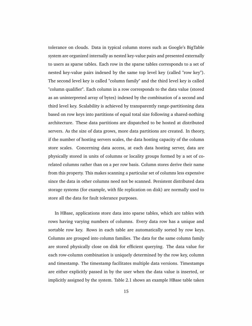
In HBase, applications store data into sparse tables, which are tables with

rows having varying numbers of columns. Every data row has a unique and

sortable row key. Rows in each table are automatically sorted by row keys.

Columns are grouped into column families. The data for the same column family

are stored physically close on disk for efficient querying. The data value for

each row-column combination is uniquely determined by the row key, column

and timestamp. The timestamp facilitates multiple data versions. Timestamps

are either explicitly passed in by the user when the data value is inserted, or

implicitly assigned by the system. Table 2.1 shows an example HBase table taken

15

Table 2.1: An example HBase table taken from the HBase website (slightly

modified). A column is specified by the concatenation of a column family name

and a column qualifier. For example, in the first column, "anchor" is the name

of a column family and "cnnsi.com" is a column qualifier. The symbols "ts8" and

"ts9" denote timestamps.

Row Key anchor: cnnsi.com anchor: my.look.ca

com.cnn ts9: cnn ts9: cnn.com

ts8: bbc.com

from the HBase website (slightly modified). The table contains one row with

row key "com.cnn" and columns "anchor: cnnsi.com" and "anchor:my.look.ca"

grouped by column family "anchor:". Each HBase row-column pair, for example,

row "com.cnn" and column "anchor:my.look.ca", is assigned a timestamp (a Java

Long type number).

HBase employs a master-slave topology. Tables are split horizontally for

distributed storage into row-wise "regions". The regions are stored on slave

machines called "region servers". Each region server hosts distinct row regions

with region data stored in persistent storage (HDFS). A pool of multiple masters

is supported eliminating a single point of failure. When a region server fails, its

data can be recovered from HDFS and be hosted by a new replacement region

server. The scalability of HBase is attributed to the shared-nothing architecture

of data regions hosted by distributed region servers. However, there could still be

bottlenecks in the system in the case when a single region server gets overloaded

by too many requests on the same data region. In fact, at each region server, all

the read/write requests to a particular row in a table region are serialized.

Currently, only simple queries using row keys and timestamps are supported in

HBase, with no SQL or join queries. It is also possible to scan and iterate through

a set of columns row by row within a row range. However inadequate the query

16

capability may seem, if the tables are formulated properly, some efficient problem-

specific search methods can be developed, especially for data with graph-like

structures such as directed acyclic graphs for workflows, which is the topic of

Chapter 4.

17

Chapter 3

Preliminary and Supportive Work

3.1 Research Overview

The PhD research project reported on in this thesis started in September 2006.

At that time, cloud computing was just emerging as a concept and the term "grid

computing" was still used more commonly. The author’s first research project was

on the "GridBASE" system [11]. GridBASE is a previously developed database-

driven light-weight distributed job execution system for running task-farmable

applications on clusters/grids. The core concept behind GridBASE is to use

computing power on-demand in a similar way to how electricity is provided in

a power grid, treating every node in the system as homogeneous. The author

refined GridBASE’s coding in terms of modularity and portability to use other

database systems rather than Oracle alone, and demonstrated its applicability

in [11] and [10]. The application of GridBASE to RNA folding, a real-world

large-scale bioinformatics application, resulted in a journal paper [25]. This

project raised the author’s interest in cloud computing which shares a similar

philosophy of using resources on-demand. The next step was to investigate

Google’s MapReduce framework and its at that time newly-developed open

19

source implementation - Hadoop.

The initial Hadoop project [45] was a case study on live cell image process-

ing. It tackled the problem of executing legacy applications (MATLAB) with

non-standard Hadoop input formats (i.e. image files instead of textual inputs)

through the Hadoop MapReduce framework. The legacy applications were exe-

cuted by Map-only MapReduce program wrappers scheduled through Hadoop

based on program execution and file staging metadata maintained in HBase. This

research was one of the earliest efforts to apply Hadoop to large-scale scientific

data processing, since early Hadoop applications were focused on server side

computations such as web indexing, etc. The method to execute MATLAB applica-

tions in a MapReduce environment in this case study is also used in later projects

to execute general legacy applications/scripts that can be invoked through simple

commandline execution.

Through the previous study, the author discovered the need for a Hadoop-

based data processing framework that is backward compatible with legacy appli-

cations and easy to use for scientists lacking programming skills. This motivated

the design of CloudWF [46], a light-weight computational workflow system to

handle workflow jobs composed of multiple MapReduce/legacy applications,

which is the subject of Chapter 4. With CloudWF, workflows can be easily con-

structed using a simple workflow description method to stitch together existing

commandline invocations and scripts. This is the first workflow management sys-

tem targeted to take advantage of the Hadoop/HBase architecture for scalability,

fault tolerance and ease of use. Firstly, CloudWF does not require any centralized

workflow engine process to control the execution flow of each workflow instance.

Instead, it uses a novel way to store the workflow graph structure into HBase

sparse tables for efficient querying and workflow dependency management. In

addition, to easily farm out workflows to cloud compute nodes, CloudWF splits

each workflow instance into independently executable blocks (for program exe-

20

cution) and connectors (for file staging and event notification). Compared with

other computational workflow systems that require one workflow execution con-

troller process per workflow instance executed, CloudWF makes load balancing,

execution coordination and fault tolerance easier.

Through developing CloudWF, it was noticed that some distributed compo-

nents need to concurrently update data stored in shared tables in HBase at the

risk of generating inconsistent data. However, there wasn’t any simple transac-

tional data management system available for HBase to handle this issue. This

led the author to the design of HBaseSI, a non-intrusive client library supporting

multi-row distributed transactions with global strong snapshot isolation (SI) on

HBase, which is the subject of Chapter 5. HBaseSI is the first SI solution for

HBase, and it functions on top of bare-bones HBase rather than implementing

and deploying an extra middleware layer over HBase. It requires no changes to

server configuration and no extra programs to be deployed. Unlike traditional

ways of handling distributed transactions, HBaseSI allows clients to make commit

decisions autonomously through the client library based on transaction metadata

stored in a separate set of system tables, avoiding the need to modify existing

user tables as well as the overhead of using complicated consensus-based pro-

tocols, explicit atomic broadcast, or transactional locks on data for distributed

synchronization and concurrency control. In this way, an easy-to-employ solu-

tion is provided that is non-intrusive to server configuration and client data. A

novel distributed queuing mechanism implemented by standard HBase tables

was employed to guarantee consistent and fresh global snapshots as well as strict

global commit ordering. Consequently, the system supports non-blocking start

of transactions with fresh data snapshots and non-blocking reads. Furthermore,

HBaseSI allows transactions to perform writes to user data tables without wait-

ing till commit time, and it employs a simple and effective straggler handling

mechanism. The approach adopted for HBaseSI can be widely applied to other

21

column stores that feature similar data organization as HBase. The initial version

of the SI system was published in [48], and a significantly improved version in

[49]. It is worth noting that Google researchers published independently and at

the same time the Percolator system [36] for supporting multi-row distributed

transactions with SI on BigTable. While the systems share some important design

ideas, there are also significant differences. Additionally, Percolator relies on the

"single-row transaction" functionality specific to BigTable, and therefore cannot

directly be implemented for HBase.

Having worked extensively with Hadoop, the author found it practically

difficult to operate a Hadoop cluster on existing cluster systems because Hadoop’s

concept is incompatible with cluster batch job queuing systems. Given this,

the author designed the CloudBATCH system [47] to use Hadoop/HBase as

a cluster management system in lieu of batch job queuing systems to accept

both MapReduce and legacy batch job submissions, removing the complexity

and overhead of making the two kinds of systems compatible. CloudBATCH

provides a nice alternative to easily configure a set of resources to cater for both

MapReduce and legacy application needs.

The main contributions of this thesis, CloudWF and HBaseSI, are presented

in Chapters 4 and 5, respectively, and some details on the preliminary and

supportive work for the thesis are given in the remainder of this chapter.

3.2 Preliminary Work

3.2.1 GridBASE

As continuation of a predecessor project called TaskSpaces [9], a new grid

computing system was developed by De Sterck and collaborators, called GridBASE

[11]. The purpose of GridBASE was to make it easy to grid-enable a certain

class of (task-farmable) applications. GridBASE was designed as a lightweight

22

and portable grid computing solution. Industry-strength database technology

played a key role in the design of the framework. The general idea was to use

a database server as a central node for task and data control. More specifically,

the database was used as a reliable and remotely accessible component both

for storing and organizing the configuration information of the grid, and for

managing information related to the grid users and the jobs and tasks they submit

for execution. Users are only concerned with submitting jobs and getting results

through a simple interface that hides the heterogeneity of the grid. Scheduling

and load-balancing are taken care of automatically by the database component

which acts as a superqueue. In this way, decentralization in space and time is

achieved.

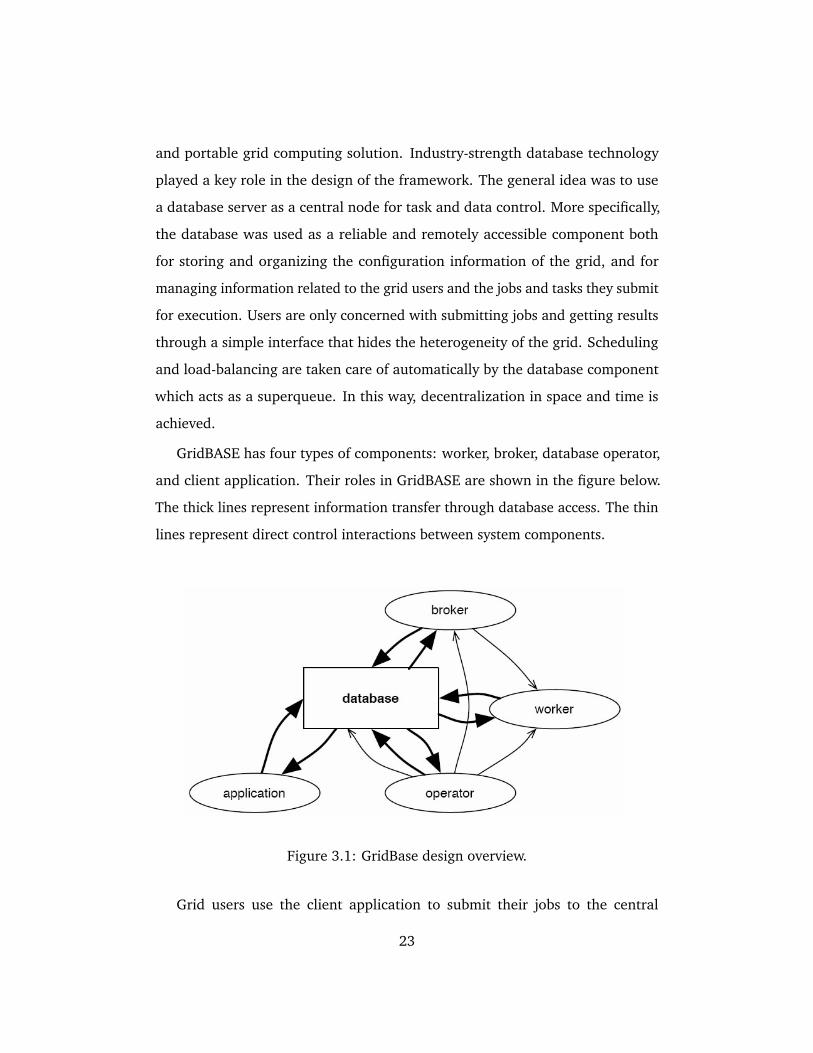
GridBASE has four types of components: worker, broker, database operator,

and client application. Their roles in GridBASE are shown in the figure below.

The thick lines represent information transfer through database access. The thin

lines represent direct control interactions between system components.

Figure 3.1: GridBase design overview.

Grid users use the client application to submit their jobs to the central

23

database. Each job is composed of tasks and their program files and input

data. Workers register with the database when they are available. Brokers period-

ically query the database and match available tasks with available workers. After

matching, brokers notify the workers that have been assigned to tasks. Workers

then download tasks from the database, execute them, and upon task completion

place the results back into the database. The "operator" role is conceptually

responsible for providing computing resources and assuring system availability

and maintenance.

GridBASE is generally suitable for users requiring the execution of big jobs

that can be decomposed into independent sub-tasks. These types of applications

are also referred to as task-farmable applications. Application code can be written

in any language, and simple workflow support is provided. In our prototype

implementation we experimented with code delivery and input and output file

delivery via the database component. Some usage scenarios are bioinformatics

problem solving, multi-tier web server hosting, web-based applications requiring

a high throughput front end and an easy-to-deploy backend, etc. The original

prototype of GridBASE was built by a former student of the research group.

The author contributed to the later phases of the GridBASE project, fixing some

system defects, rewriting part of the system and better encapsulating the database

operations of GridBASE into more extensible structures. One conference paper

[11] and one book chapter [10] were published about GridBASE.

GridBASE was a distributed computing framework that already tried to ac-

complish several goals that cloud computing environments typically target, such

as on-demand scalability, reliability, user transparency and ease of use. We used

GridBASE for distributing RNA folding tasks over a collection of clusters, and for

organizing the tasks and their input and output in collaboration with researchers

from the University of Colorado, Boulder. The results have been published in the

journal RNA [25].

24

3.2.2 Hadoop Case Studty

The GridBASE project was completed at the end of 2008. By that time, cloud

computing was starting to emerge as a promising new paradigm. As a logical

next step, we decided to explore cloud computing for scientific applications.

We performed a case study of scientific data processing using Hadoop and

published a conference paper [45]. The purpose was to explore the use of

Hadoop-based cloud computing for scientific data processing problems. At that

time, it was one of the few research efforts in the direction of applying Hadoop

to problems other than what it was designed for. We used Hadoop to develop a

simple user application that allows processing of scientific data (live cell image

files) with MATLAB on cloud nodes. The scientific data processing problem

considered in this case study is simple: the workload is divisible, without the

need for communication between tasks. There is only one processing phase,

and thus there is no need to use the "reduce" phase of Hadoop’s MapReduce.

Nevertheless, our solution relies on many of the other features offered by the

cloud concept and Hadoop, including scalability, reliability, fault-tolerance, easy

deployability, etc. At the same time, we developed a small extension to Hadoop’s

MapReduce which allows it to easily handle various input formats for scientific

data processing applications. Our approach can be generalized easily to more

complicated scientific data processing jobs (such as jobs with input data stored

in a relational database, jobs that require a reduce phase after the map phase,

scientific workflows, etc.).

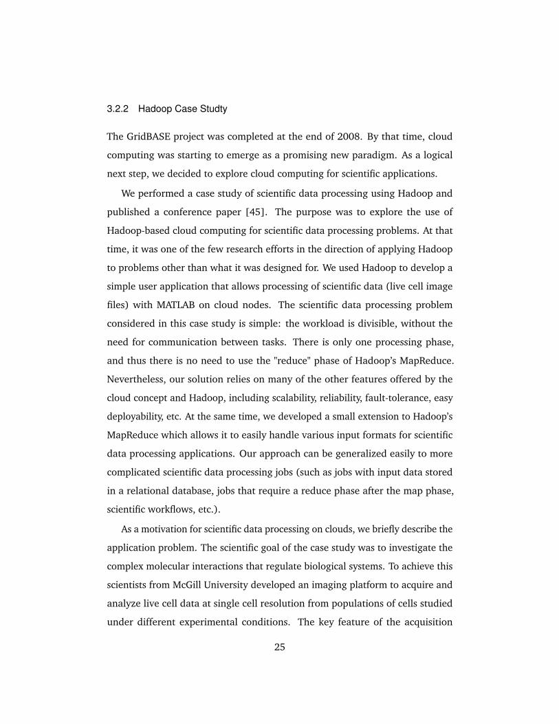
As a motivation for scientific data processing on clouds, we briefly describe the

application problem. The scientific goal of the case study was to investigate the

complex molecular interactions that regulate biological systems. To achieve this

scientists from McGill University developed an imaging platform to acquire and

analyze live cell data at single cell resolution from populations of cells studied

under different experimental conditions. The key feature of the acquisition

25

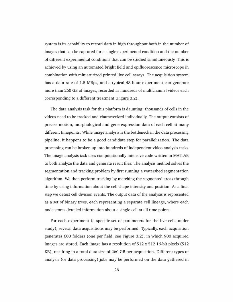
system is its capability to record data in high throughput both in the number of

images that can be captured for a single experimental condition and the number

of different experimental conditions that can be studied simultaneously. This is

achieved by using an automated bright field and epifluorescence microscope in

combination with miniaturized printed live cell assays. The acquisition system

has a data rate of 1.5 MBps, and a typical 48 hour experiment can generate

more than 260 GB of images, recorded as hundreds of multichannel videos each

corresponding to a different treatment (Figure 3.2).

The data analysis task for this platform is daunting: thousands of cells in the

videos need to be tracked and characterized individually. The output consists of

precise motion, morphological and gene expression data of each cell at many

different timepoints. While image analysis is the bottleneck in the data processing

pipeline, it happens to be a good candidate step for parallelization. The data

processing can be broken up into hundreds of independent video analysis tasks.

The image analysis task uses computationally intensive code written in MATLAB

to both analyze the data and generate result files. The analysis method solves the

segmentation and tracking problem by first running a watershed segmentation

algorithm. We then perform tracking by matching the segmented areas through

time by using information about the cell shape intensity and position. As a final

step we detect cell division events. The output data of the analysis is represented

as a set of binary trees, each representing a separate cell lineage, where each

node stores detailed information about a single cell at all time points.

For each experiment (a specific set of parameters for the live cells under

study), several data acquisitions may be performed. Typically, each acquisition

generates 600 folders (one per field, see Figure 3.2), in which 900 acquired

images are stored. Each image has a resolution of 512 x 512 16-bit pixels (512

KB), resulting in a total data size of 260 GB per acquisition. Different types of

analysis (or data processing) jobs may be performed on the data gathered in

26

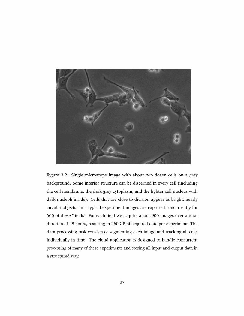
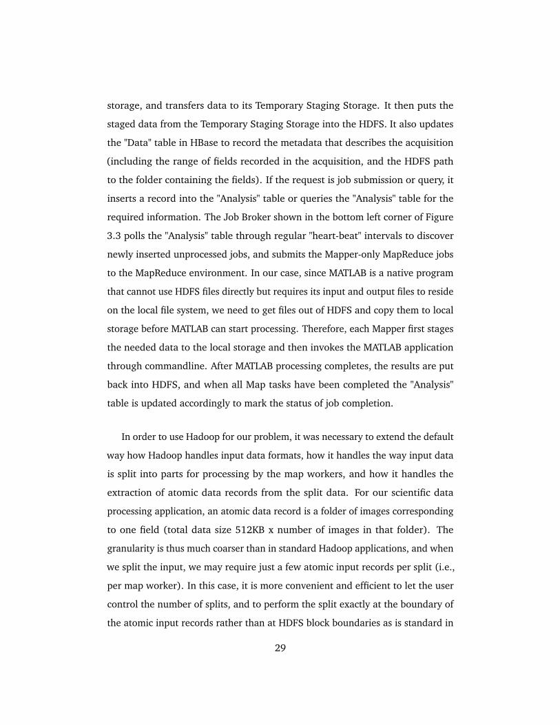
Figure 3.2: Single microscope image with about two dozen cells on a grey

background. Some interior structure can be discerned in every cell (including

the cell membrane, the dark grey cytoplasm, and the lighter cell nucleus with

dark nucleoli inside). Cells that are close to division appear as bright, nearly

circular objects. In a typical experiment images are captured concurrently for

600 of these "fields". For each field we acquire about 900 images over a total

duration of 48 hours, resulting in 260 GB of acquired data per experiment. The

data processing task consists of segmenting each image and tracking all cells

individually in time. The cloud application is designed to handle concurrent

processing of many of these experiments and storing all input and output data in

a structured way.

27

each acquisition. Analysis jobs are normally performed using MATLAB programs,

and the analysis can be parallelized easily, since each field can be processed

independently.

Client Storage

MapReduce JobTracker

HBase Master

DFS Namenode

Matlab

Local Storage

Master

Client Input

Parser

Temporary Staging Storage

Cloud Frontend

Input Results

Input Results

Client Interface

Client

Cloud Job Broker

MapReduce TaskTracker

HBase Region Server

DFS Datanode

Matlab

Local Storage

Slave

MapReduce TaskTracker

HBase Region Server

DFS Datanode

Matlab

Local Storage

Slave

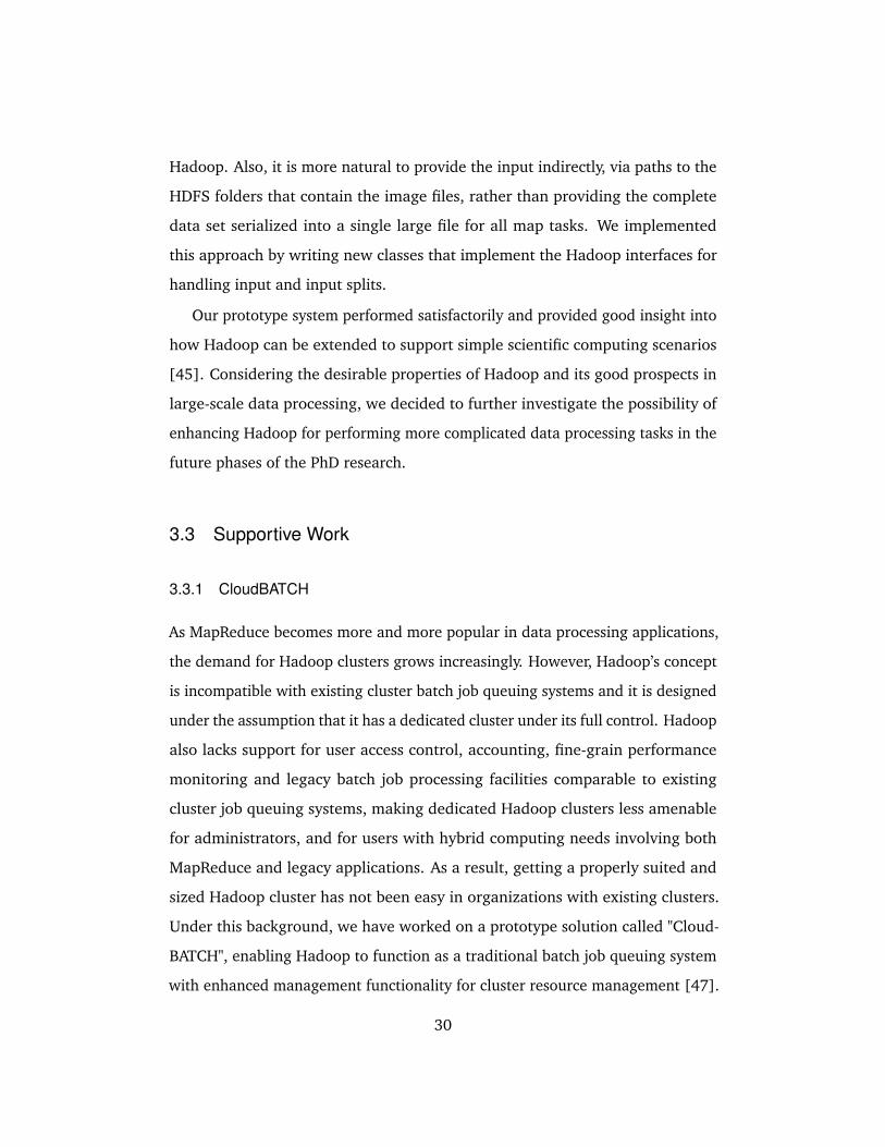
Figure 3.3: System design overview for the Hadoop case study project.

Figure 3.3 shows the design of our Hadoop-based system for processing

the data gathered in the live cell experiments. Our system puts all essential

functionality inside a cloud, while leaving only a simple Client at the experiment

side for user interaction. In the cloud, we use HDFS to store data, we use two

HBase tables, called "Data" and "Analysis", to store metadata for data and for

analysis jobs, respectively, and we use the MapReduce environment to schedule

computation. Each row in the "Data" table represents a piece of experiment data

with the path in HDFS and the data descriptions; each row in the "Analysis"

table represents an analysis job submission with its completion status. The Client

can issue three types of simple requests to the cloud application (via the Cloud

Frontend): a request for transferring experiment data (an acquisition) into the

cloud’s HDFS, a request for performing an analysis job on a certain acquisition

using a certain analysis program, and a request for querying/viewing analysis

results. The Cloud Frontend processes Client requests. When it receives a data

transfer request, it starts a Secure Copy (scp) connection to the Client’s local

28

storage, and transfers data to its Temporary Staging Storage. It then puts the

staged data from the Temporary Staging Storage into the HDFS. It also updates

the "Data" table in HBase to record the metadata that describes the acquisition

(including the range of fields recorded in the acquisition, and the HDFS path

to the folder containing the fields). If the request is job submission or query, it

inserts a record into the "Analysis" table or queries the "Analysis" table for the

required information. The Job Broker shown in the bottom left corner of Figure

3.3 polls the "Analysis" table through regular "heart-beat" intervals to discover

newly inserted unprocessed jobs, and submits the Mapper-only MapReduce jobs

to the MapReduce environment. In our case, since MATLAB is a native program

that cannot use HDFS files directly but requires its input and output files to reside

on the local file system, we need to get files out of HDFS and copy them to local

storage before MATLAB can start processing. Therefore, each Mapper first stages

the needed data to the local storage and then invokes the MATLAB application

through commandline. After MATLAB processing completes, the results are put

back into HDFS, and when all Map tasks have been completed the "Analysis"

table is updated accordingly to mark the status of job completion.

In order to use Hadoop for our problem, it was necessary to extend the default

way how Hadoop handles input data formats, how it handles the way input data

is split into parts for processing by the map workers, and how it handles the

extraction of atomic data records from the split data. For our scientific data

processing application, an atomic data record is a folder of images corresponding

to one field (total data size 512KB x number of images in that folder). The

granularity is thus much coarser than in standard Hadoop applications, and when

we split the input, we may require just a few atomic input records per split (i.e.,

per map worker). In this case, it is more convenient and efficient to let the user

control the number of splits, and to perform the split exactly at the boundary of

the atomic input records rather than at HDFS block boundaries as is standard in

29

Hadoop. Also, it is more natural to provide the input indirectly, via paths to the

HDFS folders that contain the image files, rather than providing the complete

data set serialized into a single large file for all map tasks. We implemented

this approach by writing new classes that implement the Hadoop interfaces for

handling input and input splits.

Our prototype system performed satisfactorily and provided good insight into

how Hadoop can be extended to support simple scientific computing scenarios

[45]. Considering the desirable properties of Hadoop and its good prospects in

large-scale data processing, we decided to further investigate the possibility of

enhancing Hadoop for performing more complicated data processing tasks in the

future phases of the PhD research.

3.3 Supportive Work

3.3.1 CloudBATCH

As MapReduce becomes more and more popular in data processing applications,

the demand for Hadoop clusters grows increasingly. However, Hadoop’s concept

is incompatible with existing cluster batch job queuing systems and it is designed

under the assumption that it has a dedicated cluster under its full control. Hadoop

also lacks support for user access control, accounting, fine-grain performance

monitoring and legacy batch job processing facilities comparable to existing

cluster job queuing systems, making dedicated Hadoop clusters less amenable

for administrators, and for users with hybrid computing needs involving both

MapReduce and legacy applications. As a result, getting a properly suited and

sized Hadoop cluster has not been easy in organizations with existing clusters.

Under this background, we have worked on a prototype solution called "Cloud-

BATCH", enabling Hadoop to function as a traditional batch job queuing system

with enhanced management functionality for cluster resource management [47].

30

With CloudBATCH, a complete shift to Hadoop for managing an entire cluster to

cater for hybrid computing needs becomes feasible.

There are two existing solutions to compare CloudBATCH with, each repre-

senting a typical research direction to solve Hadoop’s incompatibility issue with

legacy cluster management systems. One is Hadoop on Demand (HOD) [20],

which extends Hadoop to make it compatible with legacy systems, and the other

is Sun Grid Engine (SGE) with Hadoop integration [35], which adapts a legacy

job queuing system to make it compatible with Hadoop. However, neither of

these existing solutions are natural or elegant.

HOD is added to Hadoop for dynamically creating and using Hadoop clusters

through existing queuing systems. The idea is to make use of the existing

cluster queuing system to schedule multiple jobs that each run a Hadoop daemon

on a compute node. These running daemons together create an on-demand

Hadoop cluster. After the Hadoop cluster is set up, user-submitted MapReduce

applications can be executed. A simple walkthrough of the process for creating a

Hadoop cluster and executing user-submitted MapReduce jobs through HOD is

as follows:

1. User requests from cluster resource management system a number of nodes

on reserve and submits a job called RingMaster to be started on one of the

reserved nodes. MapReduce jobs to be executed on Hadoop cluster are

submitted as well.

2. Nodes are obtained and RingMaster is started on one of the reserved nodes.

3. RingMaster starts one process called HodRing on each of the reserved

nodes.

4. HodRing brings up on-demand Hadoop daemons (namenode, jobtracker,

tasktracker, etc.) according to the specifications maintained by RingMaster

in configuration files.

31

5. The MapReduce jobs that were originally submitted by the user are executed

on the on-demand cluster.

6. Upon completion of the MapReduce jobs, the Hadoop cluster gets torn

down and resources are released.

As seen from the above walkthrough of an HOD process, data locality of the

external HDFS is not exploited because the reservation and allocation of cluster

nodes does not take into account where the data to be processed are stored,

violating an important design principle and reducing the advantage of the MapRe-

duce framework. Another problem with HOD is that the HodRing processes are

started through ssh by RingMaster, and the cluster resource management system

is unable to track resource usage and to perform thorough cleanup when the

cluster is torn down.

SGE with Hadoop Integration is released by Oracle, enabling SGE to work

with Hadoop without requiring a separate dedicated Hadoop cluster. The core

design idea is similar to HOD in that it also tries to start an on-demand Hadoop

cluster by running Hadoop daemons through the cluster resource management

system on a set of reserved compute nodes. The difference with HOD is that SGE

takes into account data locality when scheduling tasktrackers and supports better

resource usage monitoring and cleanup because tasktrackers are directly started

by SGE as opposed to be started by HodRing in HOD. The main problem, apart

from locking users down to using SGE, lies in its mechanism of exploiting data

locality and the non-exclusive usage of compute nodes.

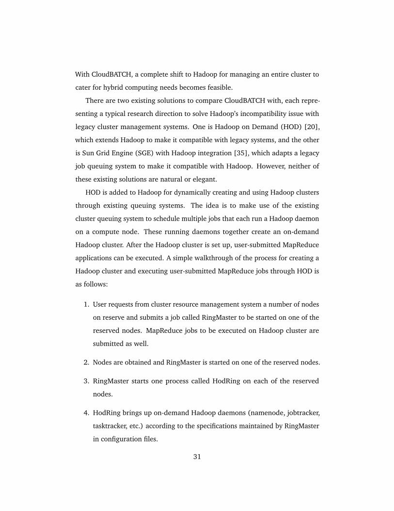
Figure 3.4 illustrates how SGE with Hadoop integration works:

1. A process called Job Submission Verifier (JSV) talks to the namenode of an

external HDFS to obtain a data locality mapping from the user submitted

MapReduce program’s HDFS paths to data node locations in blocks and

racks. Note that the "Load Sensors" are responsible for reporting on the

32

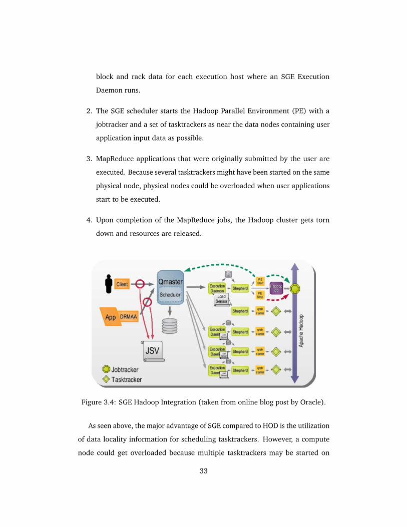
block and rack data for each execution host where an SGE Execution

Daemon runs.

2. The SGE scheduler starts the Hadoop Parallel Environment (PE) with a

jobtracker and a set of tasktrackers as near the data nodes containing user

application input data as possible.

3. MapReduce applications that were originally submitted by the user are

executed. Because several tasktrackers might have been started on the same

physical node, physical nodes could be overloaded when user applications

start to be executed.

4. Upon completion of the MapReduce jobs, the Hadoop cluster gets torn

down and resources are released.

Figure 3.4: SGE Hadoop Integration (taken from online blog post by Oracle).

As seen above, the major advantage of SGE compared to HOD is the utilization

of data locality information for scheduling tasktrackers. However, a compute

node could get overloaded because multiple tasktrackers may be started on

33

the same node for data locality concerns to execute tasks. In other words,

performance isolation is sacrificed for data locality. This type of problem was

reported by users in their real-world applications. In this case, an unpredictable

number of Hadoop speculative tasks [44] may be started on the other idling

nodes where data do not reside, incurring extra overhead in data staging and

waste of resources for executing the otherwise unnecessary duplicated tasks. The

unbalanced mingled execution of normal and speculative tasks may further mix

up Hadoop schedulers built in with the dynamically created Hadoop cluster which

are unaware of the higher level scheduling decisions made by SGE, harming

performance in unpredictable ways. Even if the default Hadoop speculative task

functionality is turned off, the potential danger of overloading a node persists,

which could further contribute to unbalanced executions of Map tasks that result

in wasting cluster resources as explained below. SGE also has an exclusive host

access facility. But if this facility is required, then the data locality exploitation

mechanism would be much less useful because normally a data node would

potentially host data blocks needed by several user applications while only one

of them can benefit from data locality in the case with exclusive host access.

Most importantly, both HOD and SGE suffer from the same major problem

intrinsic to the idea of creating a Hadoop cluster on-the-fly for each user MapRe-

duce application request. The problem is a possible significant waste of resources

in the Reduce phase, where nodes might be idling when the number of Reduce

tasks to be executed is much smaller than the number of Map tasks that were

executed in the first stage. This is because each of the on-demand clusters is

privately tailored to a single user MapReduce application submission and the size

of the Hadoop cluster is fixed at node reservation time. If the user MapReduce

application requires far more Map tasks than Reduce tasks and the number of

nodes are reserved matching the Map tasks (which is usually what users would

request), many of the machines in the on-demand Hadoop cluster will be idling

34

when the much smaller number of Reduce tasks are running at the end. The

waste of resources could also occur in the case of having unbalanced executions

of Map tasks, in which case a portion of Map tasks get finished ahead of time

and wait for the others to finish before being able to enter the Reduce phase.

On a dedicated Hadoop cluster, all these effects are smoothed out because it

typically processes multiple MapReduce jobs from multiple users at the same

time, resulting in much higher efficiency.

JobBroker j

JobBroker i

Monitor

Submit Wrapper Execute Job

Checkstatus

Client

Serial Job

MapReduce Job

Hbase Tables

Pool of MapReduce Worker Nodes

Submit WrapperExecute Job

A

Wrapper

Wrapper

Jobx

……

Wrappern ……

poll poll

Joby

Job Table User Table Queue Table

User

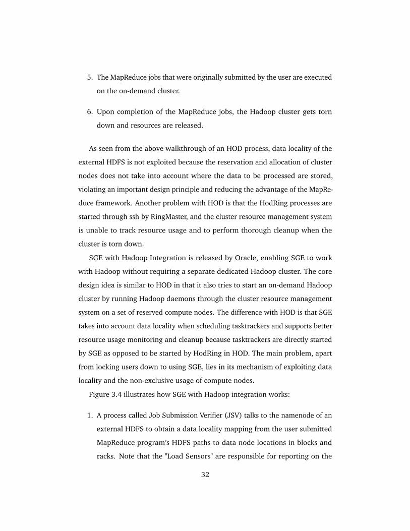
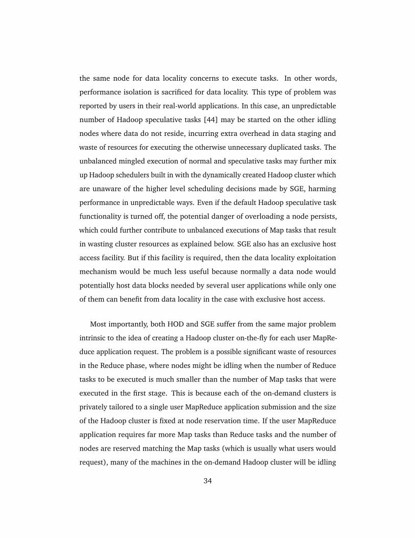
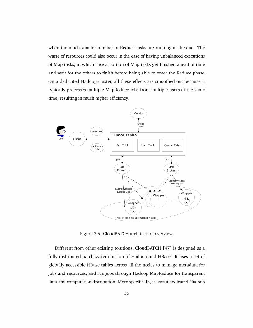
Figure 3.5: CloudBATCH architecture overview.

Different from other existing solutions, CloudBATCH [47] is designed as a

fully distributed batch system on top of Hadoop and HBase. It uses a set of

globally accessible HBase tables across all the nodes to manage metadata for

jobs and resources, and run jobs through Hadoop MapReduce for transparent

data and computation distribution. More specifically, it uses a dedicated Hadoop

35

cluster to avoid the efficiency problems identified above, it enables simple legacy

applications by a commandline approach, and it adds basic user access control

and accounting. Figure 3.5 shows the architecture overview of the CloudBATCH

system. CloudBATCH has several distributed components: Clients, Job Brokers,

Wrappers and Monitors. The general sequence of job submission and execution

using CloudBATCH is as follows: Users use Clients to submit jobs to the system.

Job information with proper job status is put into HBase tables by the Client.

In the meantime, a number of Job Brokers are polling for the HBase tables to

find jobs ready for execution. If a job is ready, a Wrapper containing the job is

submitted to Hadoop MapReduce by the Job Broker. The Wrapper is responsible

for executing the job through commandline invocation and monitoring the exe-

cution status of the job as well as updating relevant records concerning job and

resource information in HBase tables. The Wrapper is also responsible for enforc-

ing some job policies such as execution time limit. Monitors are responsible for

detecting and handling failures after Wrappers are submitted to Hadoop. Since

CloudBATCH is not a focus of this thesis, the interested reader is referred to [47]

for further details, and we suffice here with the above discussion illustrating the

difficulties of integrating MapReduce and legacy applications and outlining some

possible approaches.

36

Chapter 4

CloudWF

This chapter describes CloudWF, the first lightweight computational workflow

system naturally integrated with the Hadoop MapReduce environment for build-

ing and running computational workflows composed of both MapReduce and

existing legacy programs on Hadoop clouds. It directly inherits several desirable

properties from Hadoop, such as fault tolerance and scalability in terms of data

size. The major novelty of the CloudWF design lies in several aspects: a simple

workflow description method that encodes workflow blocks and block-to-block

dependencies separately as standalone executable components, making it easy to

reuse existing workflow components and perform runtime workflow structure

change; a file relaying mechanism through the use of HDFS, achieving automatic

and transparent file staging between connected workflow blocks; a new workflow

storage method that uses HBase to store workflow information for efficient work-

flow block dependency reconstruction at runtime, enabling multiple workflow

instances to be executed concurrently with no need for a director per workflow

instance which incurs less resource utilization per workflow instance execution.

37

4.1 Introduction

Due to the scalability, fault tolerance, transparency and easy deployability in-

herent in the cloud computing concept, Hadoop has proven highly successful in

the context of the processing of very large data sets that can be divided easily

in parts that can be processed with limited inter-task communication. However,

Hadoop does not support workflow jobs and there exist no well-established

computational workflow systems on top of Hadoop for automatic execution of

complex workflows with large data sets in a cloud environment.

Computational workflows are essential in scientific application scenarios. The

main purpose of computational workflows is to streamline and automate complex

computational processes that require multiple interdependent computing steps

and data staging in between. In general, computational workflows are directed

graphs where the nodes represent computational components and the edges

represent the temporal order of component executions as well as the data that

flow between components. The particular type of computational workflow we

target is described as follows:

1. Each workflow is represented as a directed acyclic graph (DAG). Nodes

in a DAG are called "blocks"; edges are called "connectors". Each block

represents a single executable program. Each connector represents either

the data staging between the connected blocks or just the temporal order

of block executions (dependencies).

2. The executable program in each block is either a Hadoop MapReduce

program or an existing legacy program (programs not built by using the

Hadoop MapReduce API) such as a FORTRAN or MATLAB program, invoked

by a commandline command or script.

3. A block can only become active and start execution once, not before all

38

the block’s incoming connectors finish execution. This is different from

dataflow applications where every block is scheduled to start running at

the beginning and stays active at all times, waiting for input data. In this

thesis, we distinguish dataflows from workflows by this trait.

Many scientific workflow systems on clusters and grids exist for various usage

needs such as the systems described in [27, 29, 30, 13], see also the review paper

[43]. With the advent of cloud computing, those existing systems still work well

according to their design if clouds are used in the same way as clusters and grids

[24]. However, it is not easy to deploy those systems on top of newly developed

cloud computing frameworks such as Hadoop and make them work well. This

is because the new cloud computing frameworks and the existing systems are

designed with different emphasis under different backgrounds. The new cloud

computing frameworks emphasize massive scalability and fault tolerance. As a

result, they normally employ simplifications in resource management and job

scheduling policies, such as providing users with dedicated and homogeneous

resources within a single Virtual Organization (VO) [17], providing a distributed

file system to remove the need for manual file transfer between cloud compute

nodes with various protocols (such as ftp, sftp, etc.), and hiding away as many

details of the underlying resources as possible (such as machine locations and

configurations) so that complex resource discovery and reservation due to re-

source heterogeneity are no longer necessary. Indeed, faced by peta-scale data

processing needs with easy-to-access machines at very large scales (for example,

machines provided by Amazon [15]), the paramount issue now is how to simply

run data processing jobs worry-free. On the contrary, the existing systems are de-

signed for use on clusters and grids, and emphasize orchestrating heterogeneous

resources that are each of limited scale with various hardware and software

configurations. As a result, the workflow execution mechanisms of the existing

systems need to be designed to handle the complexity and heterogeneity of the

39

resources, requiring a lot of detailed information about the underlying computing

environments for resource management and job scheduling to obtain optimized

performance on workflow executions, which would become further complicated

in large-scale systems where managing dynamic resource information in real-time

for each participating node is very difficult. Clouds provide better solutions for

these issues. Additionally, for example, the systems described in [27, 29, 30] all

need a workflow execution director role for every running workflow instance

for managing the resource mapping and execution sequence of workflow com-

ponents, which means extra resources are needed for running the director. The

directors may become performance bottlenecks especially when handling many

concurrent and large-scale workflow executions. Most importantly, existing work-

flow solutions do not easily handle Hadoop MapReduce jobs since the required

Hadoop clusters are not compatible with the queuing systems that most existing

workflow solutions are designed around.

Currently, there exist no well-established cloud environment computational

workflow systems on top of Hadoop to easily build and run computational

workflows composed of MapReduce and existing legacy programs (See Section

4.4). Our research was motivated by the lack of workflow systems in Hadoop

concerning the type of workflow applications we target, and the need for such a

system for automating large-scale data processing tasks in various fields, such

as bioinformatics, space weather simulation, phone-log processing, etc. Our

CloudWF system was designed with the following target use case in mind: A

group of scientists collaborating in a research lab frequently runs workflows of

existing scientific applications (divisible or MapReducible workloads) with large

data volumes. What CloudWF wants to achieve is to provide scientists who set

up a private cloud on their lab cluster or use public cloud resources, with an easy

way to build and execute workflows transparently on their cloud.

CloudWF is a lightweight computational workflow system for clouds based

40

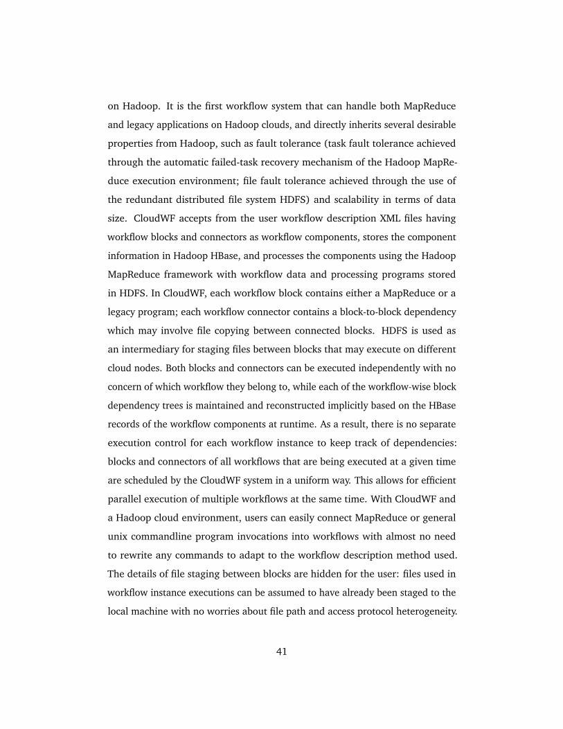
on Hadoop. It is the first workflow system that can handle both MapReduce

and legacy applications on Hadoop clouds, and directly inherits several desirable

properties from Hadoop, such as fault tolerance (task fault tolerance achieved

through the automatic failed-task recovery mechanism of the Hadoop MapRe-

duce execution environment; file fault tolerance achieved through the use of

the redundant distributed file system HDFS) and scalability in terms of data

size. CloudWF accepts from the user workflow description XML files having

workflow blocks and connectors as workflow components, stores the component

information in Hadoop HBase, and processes the components using the Hadoop

MapReduce framework with workflow data and processing programs stored

in HDFS. In CloudWF, each workflow block contains either a MapReduce or a

legacy program; each workflow connector contains a block-to-block dependency

which may involve file copying between connected blocks. HDFS is used as

an intermediary for staging files between blocks that may execute on different

cloud nodes. Both blocks and connectors can be executed independently with no

concern of which workflow they belong to, while each of the workflow-wise block

dependency trees is maintained and reconstructed implicitly based on the HBase

records of the workflow components at runtime. As a result, there is no separate

execution control for each workflow instance to keep track of dependencies:

blocks and connectors of all workflows that are being executed at a given time

are scheduled by the CloudWF system in a uniform way. This allows for efficient

parallel execution of multiple workflows at the same time. With CloudWF and

a Hadoop cloud environment, users can easily connect MapReduce or general

unix commandline program invocations into workflows with almost no need

to rewrite any commands to adapt to the workflow description method used.

The details of file staging between blocks are hidden for the user: files used in

workflow instance executions can be assumed to have already been staged to the

local machine with no worries about file path and access protocol heterogeneity.

41

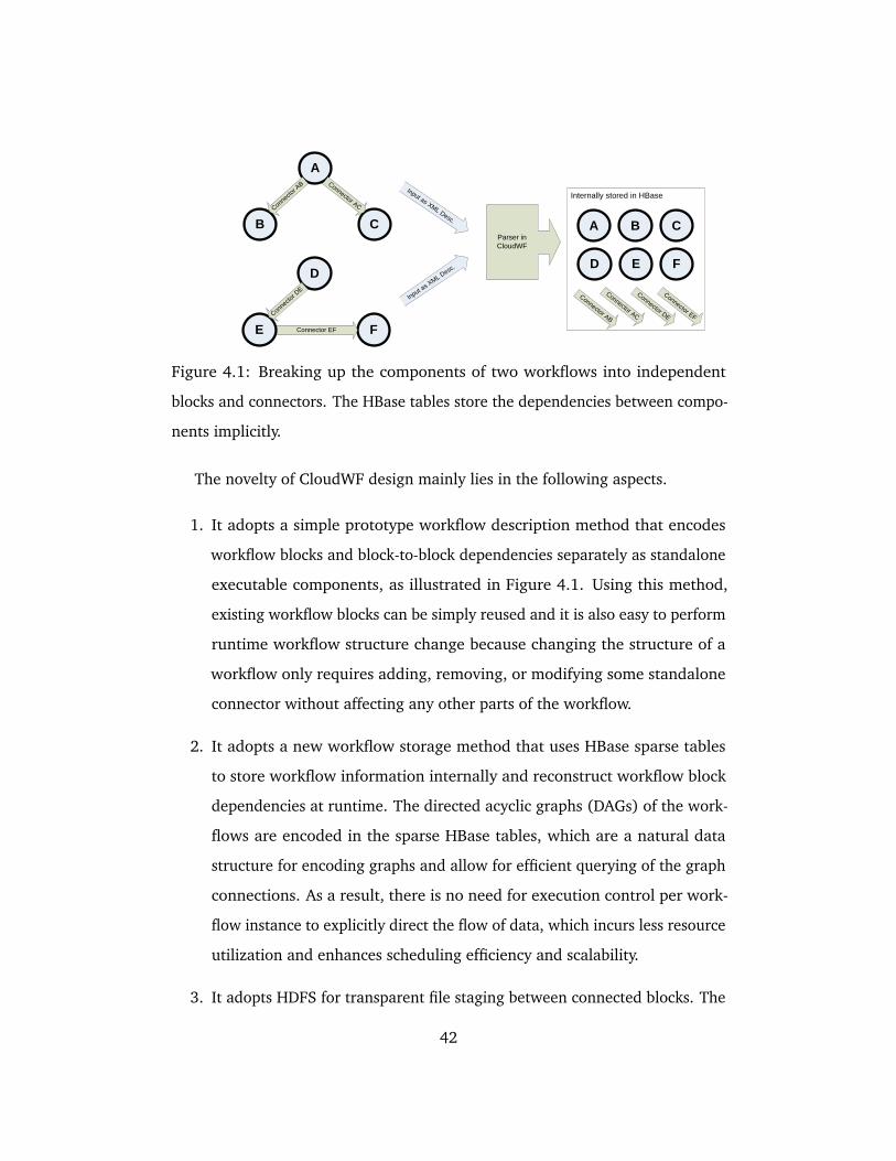
A

C

Connector AC

BConn

ector

AB

D

FConnector EFECon

necto

r DE

Parser in CloudWF

Input as XML Desc.

Input as X

ML Desc

. FED

CBA

Connector EF

Connector DE

Connector AC

Connector AB

Internally stored in HBase

Figure 4.1: Breaking up the components of two workflows into independent

blocks and connectors. The HBase tables store the dependencies between compo-

nents implicitly.

The novelty of CloudWF design mainly lies in the following aspects.

1. It adopts a simple prototype workflow description method that encodes

workflow blocks and block-to-block dependencies separately as standalone

executable components, as illustrated in Figure 4.1. Using this method,

existing workflow blocks can be simply reused and it is also easy to perform

runtime workflow structure change because changing the structure of a

workflow only requires adding, removing, or modifying some standalone

connector without affecting any other parts of the workflow.

2. It adopts a new workflow storage method that uses HBase sparse tables

to store workflow information internally and reconstruct workflow block

dependencies at runtime. The directed acyclic graphs (DAGs) of the work-

flows are encoded in the sparse HBase tables, which are a natural data

structure for encoding graphs and allow for efficient querying of the graph

connections. As a result, there is no need for execution control per work-

flow instance to explicitly direct the flow of data, which incurs less resource

utilization and enhances scheduling efficiency and scalability.

3. It adopts HDFS for transparent file staging between connected blocks. The

42

CloudWF system handles file relaying and re-naming in the background,

isolated from users. Because of employing HDFS, users and the workflow

system have a globally accessible file repository. Using HDFS to store and

relay files is convenient and reduces the complexity of handling files in a

distributed environment: the uniformity of the cloud environment allows

for simple file handling solutions.

4. It uses Hadoop’s MapReduce framework for simple scheduling and task

level fault tolerance. This avoids conflicting schedules as described in

[39] and allows for a seamless integration of both MapReduce and legacy

applications: MapReduce applications can naturally run on Hadoop while

legacy applications can be simply executed by Map-only MapReduce jobs

with the Mappers calling the legacy applications through commandline

invocation.

The remaining sections of this chapter are organized as follows. Section 4.2

describes the design and implementation of the CloudWF system in detail. Section

4.3 briefly describes an application usage scenario, followed by a discussion of

related work in Section 4.4. Section 4.5 gives conclusions and describes future

work.

4.2 CloudWF

As shown in Figure 4.2, CloudWF puts all essential functionalities inside a cloud,

while leaving the user with a very simple interface for submitting workflow XML

description files for specification of workflows, and commands to start workflows

and monitor their execution. The user also has to place any input and program

files into the user area of the cloud HDFS, and can retrieve workflow output from

the HDFS as well. (Note that the HDFS is divided into two parts, a system part

that is used by CloudWF to relay files between workflow blocks, and a user part

43

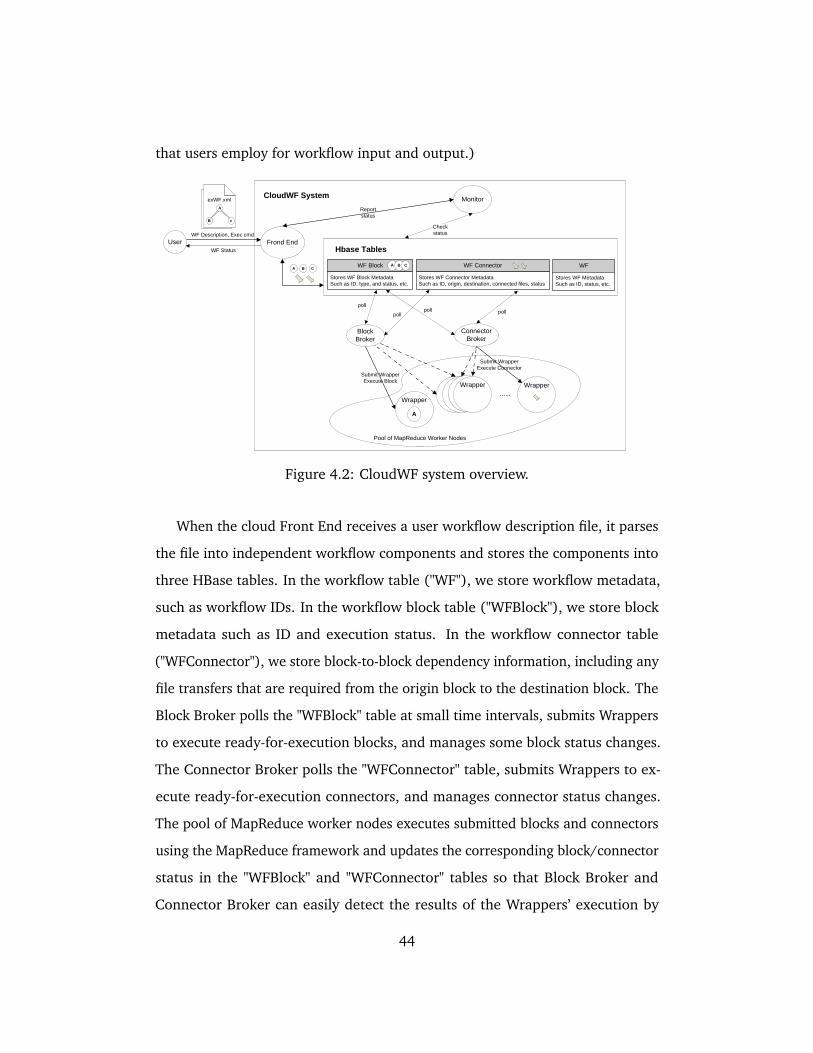
that users employ for workflow input and output.)

CloudWF System

Connector Broker

User

Block Broker

Monitor

WF Description, Exec cmd

WF Connector

Stores WF Connector MetadataSuch as ID, origin, destination, connected files, status

WF

Stores WF MetadataSuch as ID, status, etc.

WF Block

Stores WF Block MetadataSuch as ID, type, and status, etc.

Submit Wrapper Execute Block

Checkstatus

Frond EndWF Status

exWF.xml

A

zB

exWF.xmlA

cB

A B CA B C

Hbase Tables

Report status

Pool of MapReduce Worker Nodes

Submit WrapperExecute Connector

A

Wrapper

Wrapper

A ……

Wrapper……

poll

pollpoll poll

Figure 4.2: CloudWF system overview.

When the cloud Front End receives a user workflow description file, it parses

the file into independent workflow components and stores the components into

three HBase tables. In the workflow table ("WF"), we store workflow metadata,

such as workflow IDs. In the workflow block table ("WFBlock"), we store block

metadata such as ID and execution status. In the workflow connector table

("WFConnector"), we store block-to-block dependency information, including any

file transfers that are required from the origin block to the destination block. The

Block Broker polls the "WFBlock" table at small time intervals, submits Wrappers

to execute ready-for-execution blocks, and manages some block status changes.

The Connector Broker polls the "WFConnector" table, submits Wrappers to ex-

ecute ready-for-execution connectors, and manages connector status changes.

The pool of MapReduce worker nodes executes submitted blocks and connectors

using the MapReduce framework and updates the corresponding block/connector

status in the "WFBlock" and "WFConnector" tables so that Block Broker and

Connector Broker can easily detect the results of the Wrappers’ execution by

44

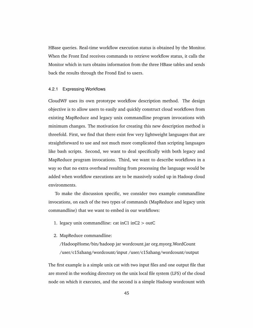
HBase queries. Real-time workflow execution status is obtained by the Monitor.

When the Front End receives commands to retrieve workflow status, it calls the

Monitor which in turn obtains information from the three HBase tables and sends

back the results through the Frond End to users.

4.2.1 Expressing Workflows

CloudWF uses its own prototype workflow description method. The design

objective is to allow users to easily and quickly construct cloud workflows from

existing MapReduce and legacy unix commandline program invocations with

minimum changes. The motivation for creating this new description method is

threefold. First, we find that there exist few very lightweight languages that are

straightforward to use and not much more complicated than scripting languages

like bash scripts. Second, we want to deal specifically with both legacy and

MapReduce program invocations. Third, we want to describe workflows in a

way so that no extra overhead resulting from processing the language would be

added when workflow executions are to be massively scaled up in Hadoop cloud

environments.

To make the discussion specific, we consider two example commandline

invocations, on each of the two types of commands (MapReduce and legacy unix

commandline) that we want to embed in our workflows:

1. legacy unix commandline: cat inC1 inC2 > outC

2. MapReduce commandline:

/HadoopHome/bin/hadoop jar wordcount.jar org.myorg.WordCount

/user/c15zhang/wordcount/input /user/c15zhang/wordcount/output

The first example is a simple unix cat with two input files and one output file that

are stored in the working directory on the unix local file system (LFS) of the cloud

node on which it executes, and the second is a simple Hadoop wordcount with

45

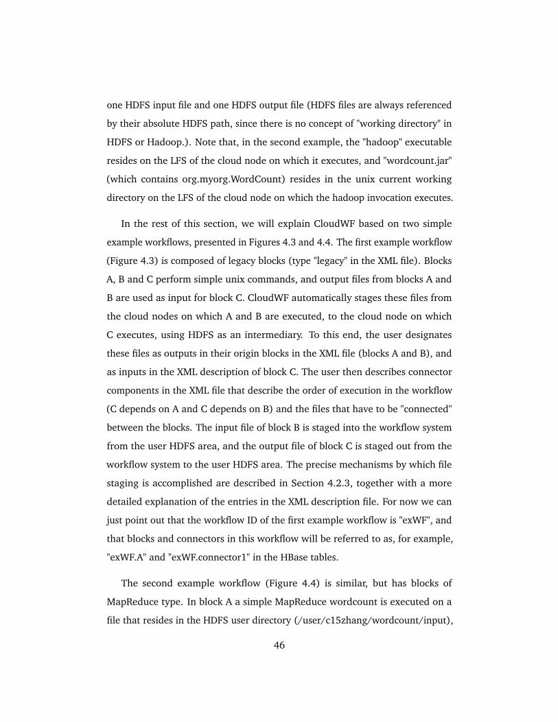
one HDFS input file and one HDFS output file (HDFS files are always referenced

by their absolute HDFS path, since there is no concept of "working directory" in

HDFS or Hadoop.). Note that, in the second example, the "hadoop" executable

resides on the LFS of the cloud node on which it executes, and "wordcount.jar"

(which contains org.myorg.WordCount) resides in the unix current working

directory on the LFS of the cloud node on which the hadoop invocation executes.

In the rest of this section, we will explain CloudWF based on two simple

example workflows, presented in Figures 4.3 and 4.4. The first example workflow

(Figure 4.3) is composed of legacy blocks (type "legacy" in the XML file). Blocks

A, B and C perform simple unix commands, and output files from blocks A and

B are used as input for block C. CloudWF automatically stages these files from

the cloud nodes on which A and B are executed, to the cloud node on which

C executes, using HDFS as an intermediary. To this end, the user designates

these files as outputs in their origin blocks in the XML file (blocks A and B), and

as inputs in the XML description of block C. The user then describes connector

components in the XML file that describe the order of execution in the workflow

(C depends on A and C depends on B) and the files that have to be "connected"

between the blocks. The input file of block B is staged into the workflow system

from the user HDFS area, and the output file of block C is staged out from the

workflow system to the user HDFS area. The precise mechanisms by which file

staging is accomplished are described in Section 4.2.3, together with a more

detailed explanation of the entries in the XML description file. For now we can

just point out that the workflow ID of the first example workflow is "exWF", and

that blocks and connectors in this workflow will be referred to as, for example,

"exWF.A" and "exWF.connector1" in the HBase tables.

The second example workflow (Figure 4.4) is similar, but has blocks of

MapReduce type. In block A a simple MapReduce wordcount is executed on a

file that resides in the HDFS user directory (/user/c15zhang/wordcount/input),

46

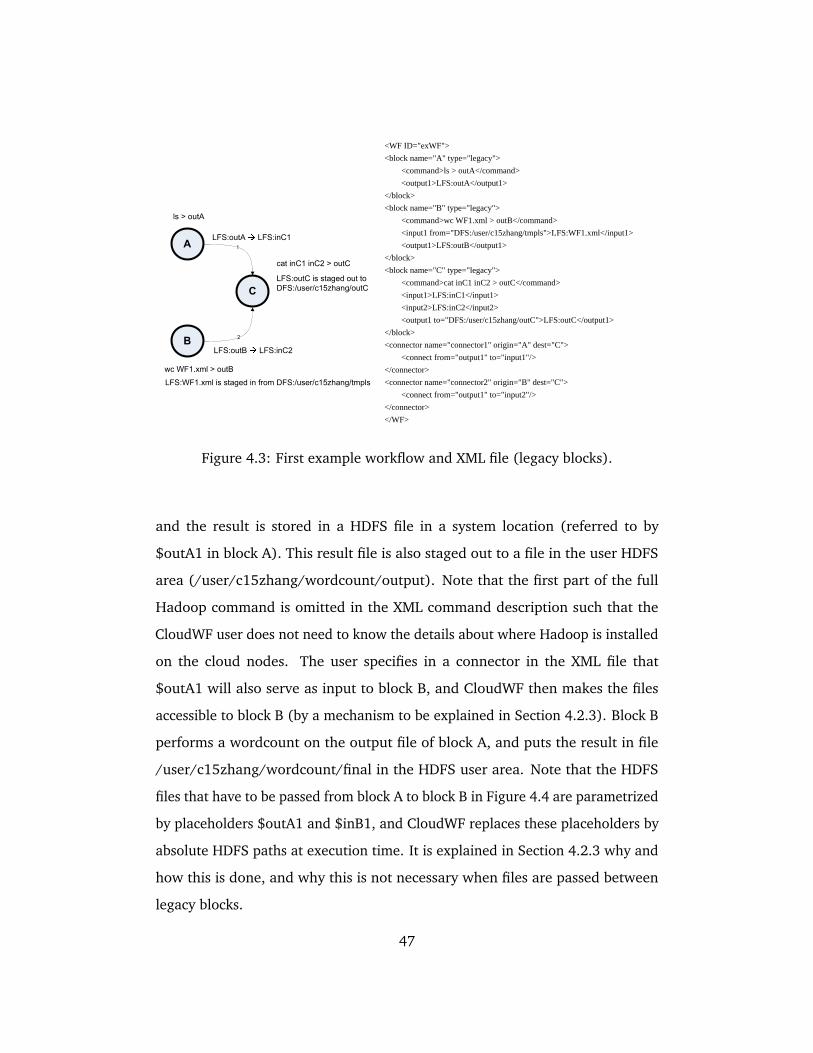
C

A 1

ls > outA

LFS:WF1.xml is staged in from DFS:/user/c15zhang/tmpls

B2

wc WF1.xml > outB

cat inC1 inC2 > outC

LFS:outA LFS:inC1

LFS:outB LFS:inC2

LFS:outC is staged out to

DFS:/user/c15zhang/outC

<WF ID="exWF">

<block name="A" type="legacy">

<command>ls > outA</command>

<output1>LFS:outA</output1>

</block>

<block name="B" type="legacy">

<command>wc WF1.xml > outB</command>

<input1 from="DFS:/user/c15zhang/tmpls">LFS:WF1.xml</input1>

<output1>LFS:outB</output1>

</block>

<block name="C" type="legacy">

<command>cat inC1 inC2 > outC</command>

<input1>LFS:inC1</input1>

<input2>LFS:inC2</input2>

<output1 to="DFS:/user/c15zhang/outC">LFS:outC</output1>

</block>

<connector name="connector1" origin="A" dest="C">

<connect from="output1" to="input1"/>

</connector>

<connector name="connector2" origin="B" dest="C">

<connect from="output1" to="input2"/>

</connector>

</WF>

Figure 4.3: First example workflow and XML file (legacy blocks).

and the result is stored in a HDFS file in a system location (referred to by

$outA1 in block A). This result file is also staged out to a file in the user HDFS

area (/user/c15zhang/wordcount/output). Note that the first part of the full

Hadoop command is omitted in the XML command description such that the

CloudWF user does not need to know the details about where Hadoop is installed

on the cloud nodes. The user specifies in a connector in the XML file that

$outA1 will also serve as input to block B, and CloudWF then makes the files

accessible to block B (by a mechanism to be explained in Section 4.2.3). Block B

performs a wordcount on the output file of block A, and puts the result in file

/user/c15zhang/wordcount/final in the HDFS user area. Note that the HDFS

files that have to be passed from block A to block B in Figure 4.4 are parametrized

by placeholders $outA1 and $inB1, and CloudWF replaces these placeholders by

absolute HDFS paths at execution time. It is explained in Section 4.2.3 why and

how this is done, and why this is not necessary when files are passed between

legacy blocks.

47

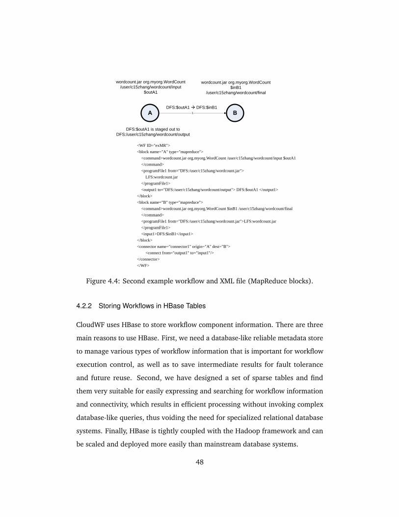
1

wordcount.jar org.myorg.WordCount /user/c15zhang/wordcount/input

$outA1

wordcount.jar org.myorg.WordCount $inB1

/user/c15zhang/wordcount/final

DFS:$outA1 DFS:$inB1

DFS:$outA1 is staged out to DFS:/user/c15zhang/wordcount/output

<WF ID="exMR">

<block name="A" type="mapreduce">

<command>wordcount.jar org.myorg.WordCount /user/c15zhang/wordcount/input $outA1

</command>

<programFile1 from="DFS:/user/c15zhang/wordcount.jar">

LFS:wordcount.jar

</programFile1>

<output1 to="DFS:/user/c15zhang/wordcount/output"> DFS:$outA1 </output1>

</block>

<block name="B" type="mapreduce">

<command>wordcount.jar org.myorg.WordCount $inB1 /user/c15zhang/wordcount/final

</command>

<programFile1 from="DFS:/user/c15zhang/wordcount.jar">LFS:wordcount.jar

</programFile1>

<input1>DFS:$inB1</input1>

</block>

<connector name="connector1" origin="A" dest="B">

<connect from="output1" to="input1"/>

</connector>

</WF>

Figure 4.4: Second example workflow and XML file (MapReduce blocks).

4.2.2 Storing Workflows in HBase Tables

CloudWF uses HBase to store workflow component information. There are three

main reasons to use HBase. First, we need a database-like reliable metadata store

to manage various types of workflow information that is important for workflow

execution control, as well as to save intermediate results for fault tolerance

and future reuse. Second, we have designed a set of sparse tables and find

them very suitable for easily expressing and searching for workflow information

and connectivity, which results in efficient processing without invoking complex

database-like queries, thus voiding the need for specialized relational database

systems. Finally, HBase is tightly coupled with the Hadoop framework and can

be scaled and deployed more easily than mainstream database systems.

48

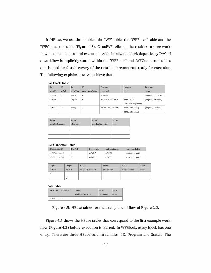
In HBase, we use three tables: the "WF" table, the "WFBlock" table and the

"WFConnector" table (Figure 4.5). CloudWF relies on these tables to store work-

flow metadata and control execution. Additionally, the block dependency DAG of

a workflow is implicitly stored within the "WFBlock" and "WFConnector" tables

and is used for fast discovery of the next block/connector ready for execution.

The following explains how we achieve that.

WFBlock Table ID:

blockID

ID:

exWF

ID:

blockType

ID:

dependencyCount

Program:

command

Program:

input

Program:

output

exWF.A Y legacy 0 ls > outA (output1,LFS:outA)

exWF.B Y Legacy 0 wc WF1.xml > outB (input1,DFS:

/user/c15zhang/tmpls)

(output1,LFS: outB)

exWF.C Y legacy 2 cat inC1 inC2 > outC (input1,LFS:inC1)

(input2,LFS:inC2)

(output1,LFS:outC)

Status:

readyForExecution

Status:

inExecution

Status:

readyForConnectors

Status:

done

WFConnector Table ID:connectorID ID:exWF Link:origin Link:destination Link:fromToList

exWF.connector1 Y exWF.A exWF.C (output1, input1)

exWF.connector2 Y exWF.B exWF.C (output1, input2)

Origin:

exWF.A

Origin:

exWF.B

Status:

readyForExecution

Status:

inExecution

Status:

readyForBlock

Status:

done

Y

Y

WF Table ID:WFID ID:exWF Status:

readyForExecution

Status:

inExecution

Status:

done

exWF Y

Figure 4.5: HBase tables for the example workflow of Figure 2.2.

Figure 4.5 shows the HBase tables that correspond to the first example work-

flow (Figure 4.3) before execution is started. In WFBlock, every block has one

entry. There are three HBase column families: ID, Program and Status. The

49

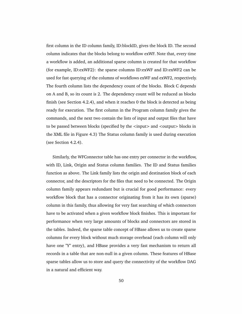
first column in the ID column family, ID:blockID, gives the block ID. The second

column indicates that the blocks belong to workflow exWF. Note that, every time

a workflow is added, an additional sparse column is created for that workflow

(for example, ID:exWF2): the sparse columns ID:exWF and ID:exWF2 can be

used for fast querying of the columns of workflows exWF and exWF2, respectively.

The fourth column lists the dependency count of the blocks. Block C depends

on A and B, so its count is 2. The dependency count will be reduced as blocks

finish (see Section 4.2.4), and when it reaches 0 the block is detected as being

ready for execution. The first column in the Program column family gives the

commands, and the next two contain the lists of input and output files that have

to be passed between blocks (specified by the <input> and <output> blocks in

the XML file in Figure 4.3) The Status column family is used during execution

(see Section 4.2.4).

Similarly, the WFConnector table has one entry per connector in the workflow,

with ID, Link, Origin and Status column families. The ID and Status families

function as above. The Link family lists the origin and destination block of each

connector, and the descriptors for the files that need to be connected. The Origin

column family appears redundant but is crucial for good performance: every

workflow block that has a connector originating from it has its own (sparse)

column in this family, thus allowing for very fast searching of which connectors

have to be activated when a given workflow block finishes. This is important for

performance when very large amounts of blocks and connectors are stored in

the tables. Indeed, the sparse table concept of HBase allows us to create sparse

columns for every block without much storage overhead (each column will only

have one "Y" entry), and HBase provides a very fast mechanism to return all

records in a table that are non-null in a given column. These features of HBase

sparse tables allow us to store and query the connectivity of the workflow DAG

in a natural and efficient way.

50

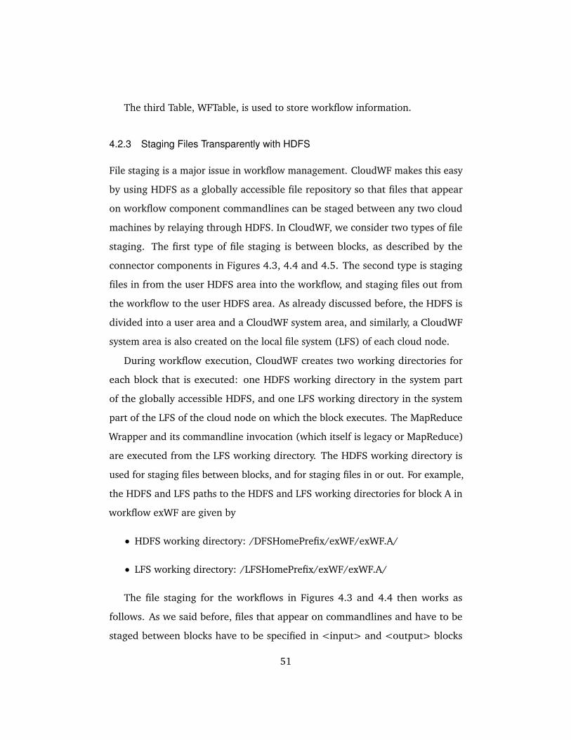
The third Table, WFTable, is used to store workflow information.

4.2.3 Staging Files Transparently with HDFS

File staging is a major issue in workflow management. CloudWF makes this easy

by using HDFS as a globally accessible file repository so that files that appear

on workflow component commandlines can be staged between any two cloud

machines by relaying through HDFS. In CloudWF, we consider two types of file

staging. The first type of file staging is between blocks, as described by the

connector components in Figures 4.3, 4.4 and 4.5. The second type is staging

files in from the user HDFS area into the workflow, and staging files out from

the workflow to the user HDFS area. As already discussed before, the HDFS is

divided into a user area and a CloudWF system area, and similarly, a CloudWF

system area is also created on the local file system (LFS) of each cloud node.

During workflow execution, CloudWF creates two working directories for

each block that is executed: one HDFS working directory in the system part

of the globally accessible HDFS, and one LFS working directory in the system

part of the LFS of the cloud node on which the block executes. The MapReduce

Wrapper and its commandline invocation (which itself is legacy or MapReduce)

are executed from the LFS working directory. The HDFS working directory is

used for staging files between blocks, and for staging files in or out. For example,

the HDFS and LFS paths to the HDFS and LFS working directories for block A in

workflow exWF are given by

• HDFS working directory: /DFSHomePrefix/exWF/exWF.A/

• LFS working directory: /LFSHomePrefix/exWF/exWF.A/

The file staging for the workflows in Figures 4.3 and 4.4 then works as

follows. As we said before, files that appear on commandlines and have to be

staged between blocks have to be specified in <input> and <output> blocks

51

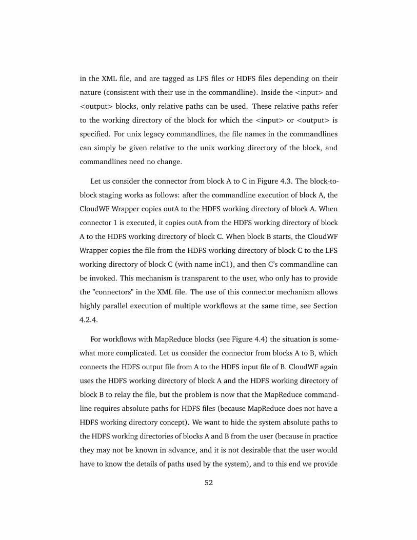
in the XML file, and are tagged as LFS files or HDFS files depending on their

nature (consistent with their use in the commandline). Inside the <input> and

<output> blocks, only relative paths can be used. These relative paths refer

to the working directory of the block for which the <input> or <output> is

specified. For unix legacy commandlines, the file names in the commandlines

can simply be given relative to the unix working directory of the block, and

commandlines need no change.

Let us consider the connector from block A to C in Figure 4.3. The block-to-

block staging works as follows: after the commandline execution of block A, the

CloudWF Wrapper copies outA to the HDFS working directory of block A. When

connector 1 is executed, it copies outA from the HDFS working directory of block

A to the HDFS working directory of block C. When block B starts, the CloudWF

Wrapper copies the file from the HDFS working directory of block C to the LFS

working directory of block C (with name inC1), and then C’s commandline can

be invoked. This mechanism is transparent to the user, who only has to provide

the "connectors" in the XML file. The use of this connector mechanism allows

highly parallel execution of multiple workflows at the same time, see Section

4.2.4.

For workflows with MapReduce blocks (see Figure 4.4) the situation is some-

what more complicated. Let us consider the connector from blocks A to B, which

connects the HDFS output file from A to the HDFS input file of B. CloudWF again

uses the HDFS working directory of block A and the HDFS working directory of

block B to relay the file, but the problem is now that the MapReduce command-

line requires absolute paths for HDFS files (because MapReduce does not have a

HDFS working directory concept). We want to hide the system absolute paths to

the HDFS working directories of blocks A and B from the user (because in practice

they may not be known in advance, and it is not desirable that the user would

have to know the details of paths used by the system), and to this end we provide

52

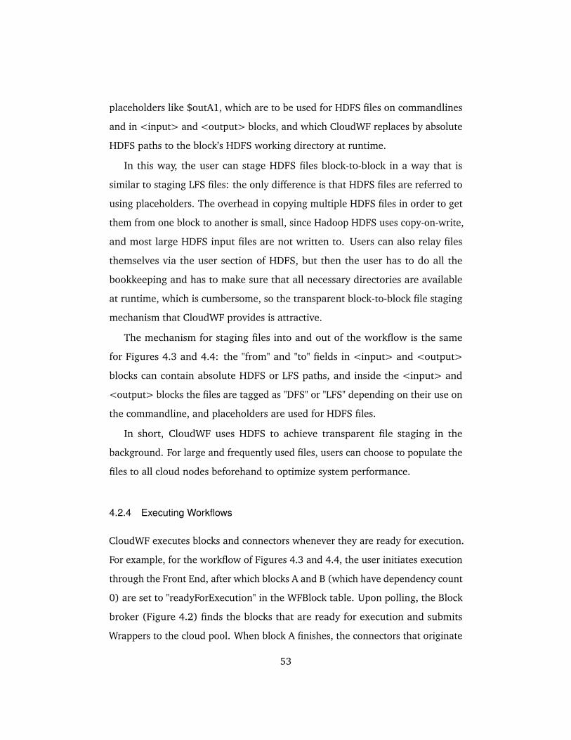
placeholders like $outA1, which are to be used for HDFS files on commandlines

and in <input> and <output> blocks, and which CloudWF replaces by absolute

HDFS paths to the block’s HDFS working directory at runtime.

In this way, the user can stage HDFS files block-to-block in a way that is

similar to staging LFS files: the only difference is that HDFS files are referred to

using placeholders. The overhead in copying multiple HDFS files in order to get

them from one block to another is small, since Hadoop HDFS uses copy-on-write,

and most large HDFS input files are not written to. Users can also relay files

themselves via the user section of HDFS, but then the user has to do all the

bookkeeping and has to make sure that all necessary directories are available

at runtime, which is cumbersome, so the transparent block-to-block file staging

mechanism that CloudWF provides is attractive.

The mechanism for staging files into and out of the workflow is the same

for Figures 4.3 and 4.4: the "from" and "to" fields in <input> and <output>

blocks can contain absolute HDFS or LFS paths, and inside the <input> and

<output> blocks the files are tagged as "DFS" or "LFS" depending on their use on

the commandline, and placeholders are used for HDFS files.

In short, CloudWF uses HDFS to achieve transparent file staging in the

background. For large and frequently used files, users can choose to populate the

files to all cloud nodes beforehand to optimize system performance.

4.2.4 Executing Workflows

CloudWF executes blocks and connectors whenever they are ready for execution.

For example, for the workflow of Figures 4.3 and 4.4, the user initiates execution

through the Front End, after which blocks A and B (which have dependency count

0) are set to "readyForExecution" in the WFBlock table. Upon polling, the Block

broker (Figure 4.2) finds the blocks that are ready for execution and submits

Wrappers to the cloud pool. When block A finishes, the connectors that originate

53

from A (obtained by a fast query of WFConnector) are set as "readyForExecution",

and are then picked up by the Connection broker and submitted for execution.

Upon completion of the connector from A to C, the dependency count of C

is decreased by one. When both connectors have executed, C then becomes

ready for execution. If any Wrapper fails, it is restarted by the MapReduce

framework automatically for six times by default. If all retries fail, the task (block

or connector) fails and thus the entire workflow fails. If the Wrapper is alive and

the submitted component execution fails, the Wrapper detects this failure and

restarts the failed component command once. If the command fails again, the

Wrapper marks the component status to fail and thus the entire workflow fails.

In the future, more advanced failure handling mechanisms will be introduced to

better cope with workflow failures.

4.2.5 Optimization: Virtual Start and End Blocks

In the prototype system, users need to explicitly start all the workflow start

blocks to kickstart the workflow execution, and the system needs to check if

all the workflow end blocks are finished to determine whether the workflow

execution is successfully completed. This is especially inefficient for workflows

with many start blocks or many end blocks. To enable easy start of workflow

execution and easy detection of successfully completed workflow execution, we

introduce virtual start and end blocks (Figure 4.6), blocks that are inserted by

the system automatically in the background to each workflow instance at the

start of execution. With virtual start blocks, starting a workflow execution can be

as easy as starting one block (the virtual start block). Likewise, detecting the end

of a workflow execution can be achieved easily by looking at the status of only

one block (the virtual end block) no matter how complex a workflow is.

54

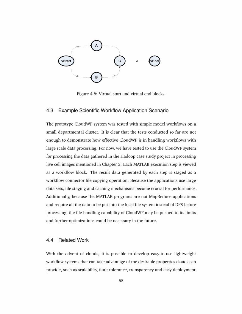
vStart C vEnd

Av1

v2

1

v3

B2

Figure 4.6: Virtual start and virtual end blocks.

4.3 Example Scientific Workflow Application Scenario

The prototype CloudWF system was tested with simple model workflows on a

small departmental cluster. It is clear that the tests conducted so far are not

enough to demonstrate how effective CloudWF is in handling workflows with

large scale data processing. For now, we have tested to use the CloudWF system

for processing the data gathered in the Hadoop case study project in processing

live cell images mentioned in Chapter 3. Each MATLAB execution step is viewed

as a workflow block. The result data generated by each step is staged as a

workflow connector file copying operation. Because the applications use large

data sets, file staging and caching mechanisms become crucial for performance.

Additionally, because the MATLAB programs are not MapReduce applications

and require all the data to be put into the local file system instead of DFS before

processing, the file handling capability of CloudWF may be pushed to its limits

and further optimizations could be necessary in the future.

4.4 Related Work

With the advent of clouds, it is possible to develop easy-to-use lightweight

workflow systems that can take advantage of the desirable properties clouds can

provide, such as scalability, fault tolerance, transparency and easy deployment.

55

Our CloudWF system tries to achieve this goal and it is the first workflow system

that can easily handle both MapReduce and legacy application executions on

Hadoop clouds.

4.4.1 Dataflow and Workflow Systems for Hadoop

At the time of writing, there exist two dataflow systems on clouds, Cascading [3]

and Pig [23], and one workflow system, Yahoo! Oozie [33], is under development.

Cascading is a dataflow system and is intended for expert programmers to build

dataflows using the provided API as monolithic programs (each dataflow instance

gets executed separately). This makes it complicated for users to reuse existing

programs directly and it is not easy to parallelize the execution of multiple

dataflows with varying length of execution (each dataflow instance needs its own

scheduler). In other words, Cascading is not intended for application users who

are not programming specialists since it does not provide a simple way to build

and run workflows by composing existing MapReduce or legacy programs without

extra programming. Pig is a platform for analyzing large data sets that provides

a high-level language called Pig Latin [31] for expressing data analysis programs.

With Pig, users can chain up data analysis jobs into dataflows. However, Pig is

not a workflow platform to work on arbitrary datasets that are not structured

into relations. In essence, Pig is designed to mimic the behavior of a relational

database in which data are organized into relations and flows of operations on

relations will output relations as well. If the data source and intermediate result

data are mostly relational and need SQL-type operations all along the dataflow,

then Pig may be a suitable platform, provided that all the relational data are

written and stored in Pig-recognized formats, and all the original SQL queries (if

they exist) or data manipulation commands are re-written using Pig Latin syntax.

Apparently, Pig is not suitable for the type of workflows we target because we

need a system that is more general and non-intrusive for cloud-enabling existing

56

legacy and MapReduce programs without any modification to those programs

and without any restriction on the type or format of data those programs are

using. Yahoo! Oozie is intended to be a comprehensive workflow management

and coordination system for Hadoop to support many different job types that

can run on clouds, such as MapReduce, Pig, Hadoop Streaming [41], HDFS, etc.

It was started at almost the same time as our computational workflow system

and became inactive shortly afterward. Its design is similar to existing workflow

systems on grids, with the exception that jobs are run on Hadoop and the job

files are put in HDFS. It hard-codes dependency in each workflow block (making

it difficult to do isolated modifications to a block and avoid implications on other

parts of the workflow) and mainly targets MapReduce-type applications (one

needs to write extra action executors to support arbitrary types of applications),

making compatibility with existing legacy programs more difficult. However, if

Oozie sees more development action in the future, it may become relevant to

what our system tries to achieve.

4.4.2 Legacy Workflow Systems

Additionally, in terms of general workflow organization, our system is novel

compared to existing major computational workflow systems in several aspects.

For ease of discussion, we re-state some of the novelties of CloudWF besides

the seamless integration with Hadoop as follows: first, it encodes workflow

blocks and block-to-block dependencies separately as standalone executable

components which enables decentralized workflow execution management, in

a way that is naturally suitable for cloud environments; second, it employs a

new way to store workflow dependencies in HBase sparse tables such that they

become efficiently searchable and enables multiple workflow instances to be

executed concurrently with no need for a separate director to drive through

each workflow instance execution; third, it uses HDFS for staging files between

57

workflow blocks transparently such that users do not need to be concerned about

specific file transfer protocols or file naming conflicts. File renaming can also be

handled automatically if applications have particular requirements on a certain

naming convention.

There are several major computational workflow systems, such as Condor

DAGMan [16], Kepler [27], and Pegasus [38], each targeted to certain usage

scenarios but none closely integrated with Hadoop for running MapReduce-type

applications.

Condor DAGMan is a workflow engine designed to manage workflows com-

posed of Condor [37] jobs. A DAGMan process is started as a normal compute job

submitted to Condor (one DAGMan process per workflow instance). Workflows

are coded as workflow description files using DAGMan’s own syntax. After an

instance of DAGMan is started, it reads a workflow description file and submits

jobs to Condor according to the block ordering determined by the workflow

dependency read from the workflow description file. It monitors the log files

for each block submission and determines based on the return values of the

finished blocks whether or not to submit the next available jobs according to the

dependency.

Kepler [27] is a GUI-based workflow composition and execution environment,

focusing on the automation of workflow Actor executions controlled by Directors.

A Kepler workflow is composed of a set of connected Actors. An Actor is an

independent functional unit, such as a program, a file transfer manager (i.e.,

a program specialized in transferring files, such as a scp file manager taking

inputs composed of a source and destination string and user password), etc. Each

Actor has a number of input/output ports. Ports belonging to different Actors

are connected by Channels. A Channel is just a GUI line drawn to connect the

ports, representing the data flow or event notification sequence. Each workflow

instance execution is controlled by one Director. The Directors are not responsible

58

for file transfers or resource mapping; such tasks are off-loaded to specialized

Actors such as file transfer Actors and grid job submission Actors. Remote

job execution on clusters and grids are done just as if by hand (explicit user

credentials and submission commands must be coded in the job submission

Actor). Furthermore, one cannot run arbitrary Actors on clusters/grids unless all

the required files of the Actors are wrapped in submission scripts acceptable for

the target clusters/grids batch job queuing system.

CloudWF is different from DAGMan and Kepler in several aspects. First, in

CloudWF, there is no need for separate director roles for each workflow instance

execution, saving valuable compute resources. Second, CloudWF stores workflow

dependencies in HBase sparse tables for efficient queries and easy workflow exe-

cution management. Third, CloudWF supports transparent and protocol neutral

file staging between blocks. Finally, CloudWF seamlessly supports both MapRe-

duce and legacy applications, while executing MapReduce jobs with DAGMan

and Kepler is not straightforward.

4.4.3 The Pegasus Workflow System

Pegasus [38] is a grid workflow system that has some conceptual similarity to

CloudWF. Therefore, we now give a more detailed comparison to Pegasus.

Pegasus is a system that allows users to write resource independent (no actual

physical file paths are included) workflow description files (called DAX - Directed

Acyclic graph workflow XML), and then automatically transforms the DAX into

DAGMan description files and submits DAGMan jobs to Condor which executes

the workflows. Figure 4.7 shows the architecture of Pegasus. Pegasus uses

Abstract Workflows, which contain resource neutral bindings for files. In other

words, no physical file paths are used in the abstract workflows but only abstract

file names. There is a central data registry containing information about the

mappings of each file to different physical paths at different compute nodes.

59

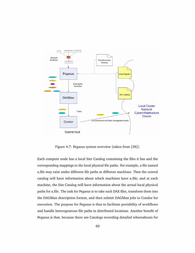
Figure 4.7: Pegasus system overview (taken from [38]).

Each compute node has a local Site Catalog containing the files it has and the

corresponding mappings to the local physical file paths. For example, a file named

a.file may exist under different file paths at different machines. Then the central

catalog will have information about which machines have a.file, and at each

machine, the Site Catalog will have information about the actual local physical

paths for a.file. The task for Pegasus is to take such DAX files, transform them into

the DAGMan description format, and then submit DAGMan jobs to Condor for

execution. The purpose for Pegasus is thus to facilitate portability of workflows

and handle heterogeneous file paths in distributed locations. Another benefit of

Pegasus is that, because there are Catologs recording detailed whereabouts for

60

all files, if a host already contains a certain file, that file can be re-used and there

is no need to stage that file multiple times when used by multiple workflows

at that host. However, users need to take care of properly naming the files and

keeping track of file changes at all replicas, which may become cumbersome.

Pegasus is somewhat similar to CloudWF in its file staging approach. Recall

that Pegasus converts abstract workflow description files to condor DAGMan files

for execution. During the conversion, Pegasus inserts data stage-in and stage-out

processes as additional separate blocks for each original workflow block if files

are to be staged. As a result, a block in the original abstract workflow may

be converted to a group of blocks containing several input staging blocks, an

executable block, and several output staging blocks. For input staging blocks, the

file catalog will be queried using the logical file identifiers and the corresponding

physical files will be staged to the local compute node. For output staging blocks,

files will be staged back to the compute node where the block’s corresponding

DAGMan job is submitted for execution and relayed to subsequent blocks as

their inputs via intermediate file storage locations when necessary. CloudWF

also uses a file relaying mechanism to stage outputs of preceding blocks to their

subsequent blocks as inputs. A difference is that Pegasus uses the local storage

of the compute node where the DAGMan job is submitted as the basis to relay

files, whereas CloudWF uses HDFS as a globally viewable and accessible file

repository to relay files. Both of the two systems can transparently relay files

between connected blocks alleviating users from the burden of hardcoding any

file staging operations by actual physical file paths combined with specific file

transfer protocols.

Pegasus is different from CloudWF in several aspects. Pegasus does not work

with Hadoop by default, whereas CloudWF naturally integrates with Hadoop

MapReduce and is oriented towards workflows composed of both legacy and

MapReduce applications. Pegasus uses DAGMan which requires an extra exe-

61

cution monitoring process per workflow instance incurring extra resource use

and the complexities concerning the scalability and fault tolerance of those mon-

itoring processes, whereas CloudWF uses a novel way to efficiently store and

manage workflow dependencies using HBase sparse tables such that there is

no need for an extra workflow director role per workflow instance to manage

the workflow execution graph. Furthermore, modifying a Pegasus workflow

would cause the entire workflow to be re-compiled and the condor submission

files to be re-generated before the new workflow can be executed, whereas the

method to treat workflow blocks and connectors as independent executables

in CloudWF makes it potentially easy to modify any block/connector without

affecting other blocks/connectors in the same workflow, even at runtime. Finally,

Pegasus requires many other heavy-weight grid tools (e.g. globus services, gridftp

on each file hosting site, condor, and many Pegasus components) to be deployed

whereas CloudWF only requires Hadoop and HBase.

4.5 Conclusions and Future Work

CloudWF is a computational workflow system specifically targeted at cloud

environments where Hadoop is installed. It uses Hadoop components for job

execution, file staging and workflow information storage. The novelty of the

system lies in several aspects: its new workflow description method that separates

out workflow component dependencies as standalone executable components

such that there is no need for execution control per workflow instance to explicitly

direct the flow of data, which improves resource utilization and enhances efficient

scheduling; the directed acyclic graphs (DAGs) of the workflows are encoded in

sparse HBase tables, which are a natural data structure for encoding graphs and

allow for efficient querying of the graph connections; using HDFS to conveniently

store and relay files reduces the complexity of handling files in a distributed

environment – the uniformity of the cloud environment allows for simple file

62

handling solutions that are fully transparent to the user.

The current prototype CloudWF system can support building and running

simple workflows composed of both MapReduce and legacy applications. Con-

cerning future work, several other advanced features are planned to be built to

further improve the prototype CloudWF system, namely:

1. Reusing workflow/block templates and nested workflows.

2. Execution steering with conditional branching and loops.

3. Runtime interactive workow change with instance clones.

CloudWF can also be extended to cloud computing frameworks other than

Hadoop, as long as there is a distributed file system providing a global view and

a metadata store like HBase supporting sparse tables.

63

Chapter 5

Snapshot Isolation for Column Stores

on Clouds

This chapter presents the "HBaseSI" client library, which provides global strong

snapshot isolation (SI) for multi-row distributed transactions in HBase. This is the

first SI mechanism developed for HBase. HBaseSI uses novel methods in handling

distributed transactional management autonomously by individual clients. These

methods greatly simplify the design of HBaseSI and can be generalized to other

column-oriented stores with similar architecture as HBase. As a result of the

simplicity in design, HBaseSI adds low overhead to HBase performance and

directly inherits many desirable properties of HBase. HBaseSI is non-intrusive to

existing HBase installations and user data, and is designed to work with a large

cloud in terms of data size and the number of nodes in the cloud.

5.1 Introduction

Column stores provide database-like table views, and it would be desirable if

distributed transactions can be supported on them so that applications that used

65

to be built around traditional database management systems (DBMS) can make

use of cloud column stores for transactional data processing, with improved scala-

bility. Indeed, many applications, such as a large number of collaborative Web 2.0

applications, would benefit from transactional multi-row access to the underlying

data stores [1]. In fact, those modern applications pose high requirements on

scalability and fault tolerance and there are currently no existing DBMS solutions

(even parallel database systems) to fully cater to those requirements due to the

overhead of managing distributed transactions and the fact that it is impossible

for DBMSs to guarantee transactional properties in the presence of various kinds

of failures without limiting system scalability and availability [1, 5, 22]. Unfortu-

nately, no out-of-the-box support for transactions involving multiple data rows

exists in column stores. This is mainly because multi-row transactions in column

stores are intrinsically distributed transactions [16] and traditional approaches,

such as standard 2-phase commit protocols [2], consensus-based commits [26],

atomic broadcast [14], and explicit data locking [7], would suffer from similar

problems as in existing distributed DBMS solutions if they are directly applied to

column stores.

This chapter presents a novel light-weight transaction system with global

strong snapshot isolation on top of HBase (which is a representative open source

column store modeled after Google’s BigTable system), without using traditional

methods of handling distributed transactions. A preliminary version of our system,

providing weak SI for HBase, was presented in [48]. The solution presented in

this chapter is called "HBaseSI". HBaseSI recycles some of the design principles

of the initial system from [48] but uses a different, more efficient solution for

handling distributed synchronization, with added support for global strong (and

not weak) SI and an efficient failure handling mechanism. Our work in [48]

described the first ever SI system for column-stores. Independently and at the

same time, the Google Percolator system was presented in [36]. Percolator

66

provides global strong SI for Google’s column store system, BigTable. Percolator

shares many design principles with our SI system, but there are also many

important differences in design goals. Several other research efforts have been

made to investigate solutions for supporting multi-row distributed transactions

on HBase (see Section 5.5). However, none of those solutions provide transaction

support with global snapshot isolation.

HBaseSI targets the same type of OLTP (Online Transaction Processing) work-

loads as HBase, taking advantage of HBase’s random data access performance. It

is implemented as a client library and does not require any extra programs to be

deployed or running in addition to existing HBase servers. In addition, HBaseSI

is non-intrusive to existing user data that have already been stored in HBase

since it does not require modifications to existing user data tables. Therefore,

it is very easy for current HBase users to employ the system for transactions on

their existing data. In HBaseSI, transactional management metadata are written

by each transaction to a separate set of HBase tables. There is no central "commit

engine" that decides which of the transactions that are ready to commit can

actually commit; instead, the transaction processes decide autonomously, in a dis-

tributed fashion, whether they can commit or have to fail, using the information

stored in the additional metadata HBase tables. As a result, little performance

overhead pertaining to distributed synchronization is added by the transactional

management logic. Many of HBase’s desirable properties are directly inherited

as well, such as fault tolerance, access transparency and high throughput. In

its current design, HBase does not target scalability in terms of the number of

transactions per unit of time.

The main contributions of HBaseSI are: 1. HBaseSI is the first distributed

transactional system with global SI for HBase. The system design can be applied

to other column stores similar to HBase, which means a broader set of applications

can use column stores, namely, the ones that need to use transactional SI;

67

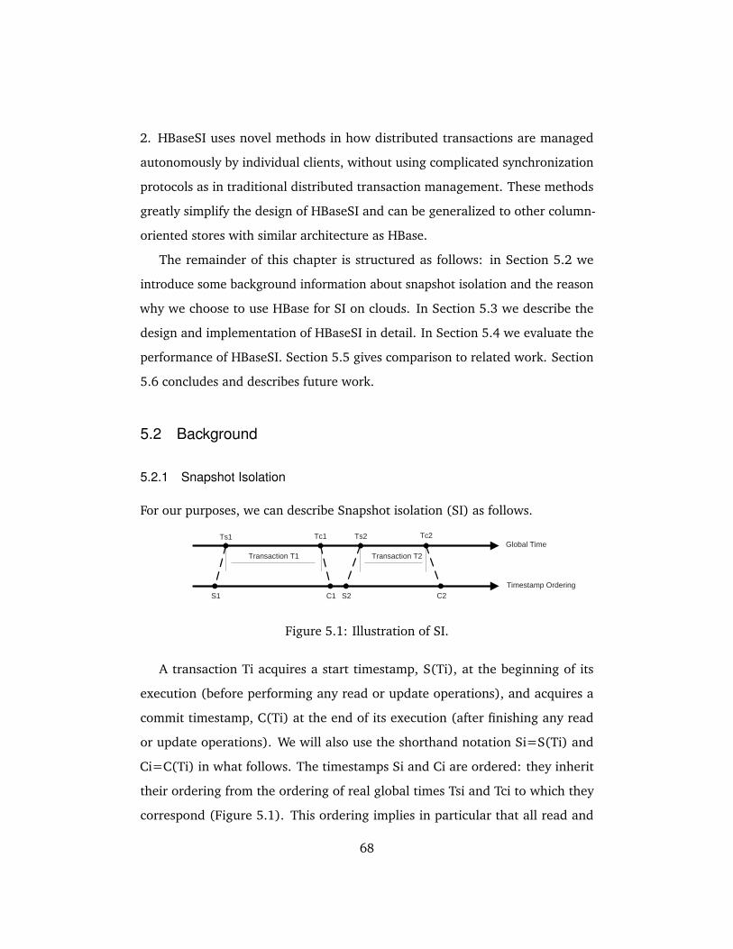
2. HBaseSI uses novel methods in how distributed transactions are managed

autonomously by individual clients, without using complicated synchronization

protocols as in traditional distributed transaction management. These methods

greatly simplify the design of HBaseSI and can be generalized to other column-

oriented stores with similar architecture as HBase.

The remainder of this chapter is structured as follows: in Section 5.2 we

introduce some background information about snapshot isolation and the reason

why we choose to use HBase for SI on clouds. In Section 5.3 we describe the

design and implementation of HBaseSI in detail. In Section 5.4 we evaluate the

performance of HBaseSI. Section 5.5 gives comparison to related work. Section

5.6 concludes and describes future work.

5.2 Background

5.2.1 Snapshot Isolation

For our purposes, we can describe Snapshot isolation (SI) as follows.

S1 C1 S2 C2Timestamp Ordering

Global TimeTs1 Tc1 Ts2 Tc2

Transaction T1 Transaction T2

Figure 5.1: Illustration of SI.

A transaction Ti acquires a start timestamp, S(Ti), at the beginning of its

execution (before performing any read or update operations), and acquires a

commit timestamp, C(Ti) at the end of its execution (after finishing any read

or update operations). We will also use the shorthand notation Si=S(Ti) and

Ci=C(Ti) in what follows. The timestamps Si and Ci are ordered: they inherit

their ordering from the ordering of real global times Tsi and Tci to which they

correspond (Figure 5.1). This ordering implies in particular that all read and

68

write operations of Ti happen (in real, global time) after the time corresponding

to Si, and all write operations of Ti happen (in real, global time) before the time

corresponding to Ci. Transactions Ti and Tj are called concurrent if their lifespan

intervals (Si,Ci) and (Sj,Cj) overlap. A transaction Ti that commits successfully is

called a successful or committed transaction.

Global Strong SI can then be described as follows. A transaction history H

satisfies global strong SI, if its (successful) transactions satisfy the following two

conditions: 1. Read operations in any transaction Ti see the database in the

state after the last commit before Si. In other words, all updates made by the

committed transaction Tj which has the last Cj <= Si are visible to Ti. However,

read operations in transaction Ti that read data items that have previously been

written by transaction Ti itself, see the data values that were last written by Ti; 2.

Concurrent transactions have disjoint writesets.

We add the qualifier "global" when we define strong SI because we want to

investigate Snapshot Isolation for a distributed system in this chapter, and want

to stress that the definition above applies to the global system. Additionally, the

above definition does not regulate the behavior when two concurrent transactions

with overlapping writesets both try to commit. In many occasions, a rule called

the "first-committer-wins" rule [19] is employed, which will cause the failure of

the transaction that is second in attempting to commit. To illustrate this rule,

let’s look at an example set of transactions as shown in Figure 5.2. T1 and

T2 must have disjoint writesets in order to both commit successfully. If they

have overlapping writesets, only T1 will successfully commit and T2 will abort,

because T1 attempts to commit before T2.

The strong notion of SI as defined above is different from the original def-

inition of SI [19], which allows Si to be chosen corresponding to any time in

the past before the first read or update operation in transaction Ti. This relaxed

version of SI is also called weak SI in [8]. To illustrate this difference, we assume

69

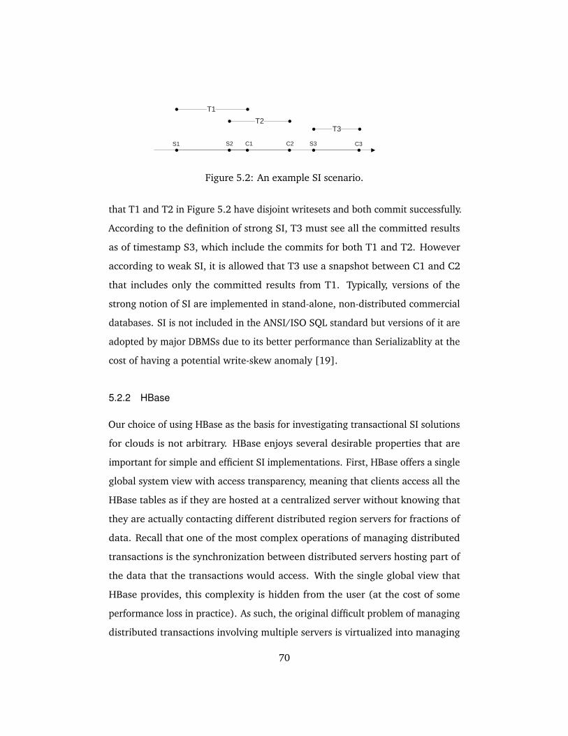
T1T2

T3

S1 C1S2 C2 S3 C3

Figure 5.2: An example SI scenario.

that T1 and T2 in Figure 5.2 have disjoint writesets and both commit successfully.

According to the definition of strong SI, T3 must see all the committed results

as of timestamp S3, which include the commits for both T1 and T2. However

according to weak SI, it is allowed that T3 use a snapshot between C1 and C2

that includes only the committed results from T1. Typically, versions of the

strong notion of SI are implemented in stand-alone, non-distributed commercial

databases. SI is not included in the ANSI/ISO SQL standard but versions of it are

adopted by major DBMSs due to its better performance than Serializablity at the

cost of having a potential write-skew anomaly [19].

5.2.2 HBase

Our choice of using HBase as the basis for investigating transactional SI solutions

for clouds is not arbitrary. HBase enjoys several desirable properties that are

important for simple and efficient SI implementations. First, HBase offers a single

global system view with access transparency, meaning that clients access all the

HBase tables as if they are hosted at a centralized server without knowing that

they are actually contacting different distributed region servers for fractions of

data. Recall that one of the most complex operations of managing distributed

transactions is the synchronization between distributed servers hosting part of

the data that the transactions would access. With the single global view that

HBase provides, this complexity is hidden from the user (at the cost of some

performance loss in practice). As such, the original difficult problem of managing

distributed transactions involving multiple servers is virtualized into managing

70

shared data access at a centralized server, significantly reducing the complexity of

transactional protocol implementation. This significantly reduces the complexity

of transactional protocol implementation. Second, HBase provides multi-version

data support distinguished by the timestamp the data item is written with. In

other words, snapshots of data identified by write timestamps are naturally kept

in HBase. This feature can directly facilitate the SI protocol implementation.

Third, HBase guarantees single atomic row operations (reads/writes) with strong

data consistency in the global table view. This means that a data item, once

successfully written, is guaranteed to show a consistent value seen globally by

all clients. This is a very important property for transactions to rely on for data

consistency. Imagine if HBase were to support only eventual data consistency in

its global table view: it would then be impossible to make clear guarantees on

the availability of any data items.

Note that HBase does not guarantee that two messages sent in a certain order

(for example, messages sent in the form of calling the insertRow method to add

a row into a global system table) will be delivered in the same order (in the form

of rows appearing in the global table), no matter whether the message sending

order is determined by real time or a centralized timestamp. More specifically, it

is possible that, if a client calls the method to insert row1 before another client

calls the method to insert row2 into the same global table, row2 appears in the

global table first. In fact, any row could take arbitrarily long to appear and it may

even never appear, with atomicity guaranteed. This is also why in the HBaseSI

protocol, we cannot solely rely on the order of data row appearance to order

arrival of transactional information in the tables.

71

5.3 HBaseSI

5.3.1 System Design

A major design goal of HBaseSI is to provide transactional SI for HBase with

minimum add-ons to existing HBase installations and administration. It may

also be an advantage if it is possible for HBase users with existing data tables

to employ HBaseSI with minimum effort. To this end, HBaseSI is implemented

as a client library in Java with no extra programs to be deployed. Applications

that need to do transactions use the client library to interact with HBase instead

of using the standard HBase API. Each transaction writes its own transactional

metadata (e.g. transaction ID, commit timestamp, commit request, etc.) to a

set of global system HBase tables (separate from existing user data tables), and

queries those tables to obtain information about other transactions. Based on the

information obtained, and by accessing this information with atomic read/write

operations provided by HBase, a transaction can autonomously decide to commit

or abort. From a user’s point of view, using HBaseSI requires no modification

to any existing data tables and only requires switching to a new client API with

semantics similar to the HBase API. From a system administrator’s point of view,

using HBaseSI incurs no change to the existing HBase administration.

HBaseSI employs several HBase tables in addition to the user’s data tables.

These additional system tables are three Counter tables (Tables 5.1, 5.2 and 5.3)

for providing globally unique counters, a CommitRequestQueue table (Table 5.4)

that acts as a queue for transactions that are submitting requests to commit, a

CommitQueue table (Table 5.5) that acts as a queue for transactions that have

been cleared to commit, and a Committed table (Table 5.6) that keeps track of

successfully committed transactions and their writesets.

The Counter tables are intended to serve as a set of centralized locations for

issuing globally unique IDs that may be used as well-ordered counters. Each

72

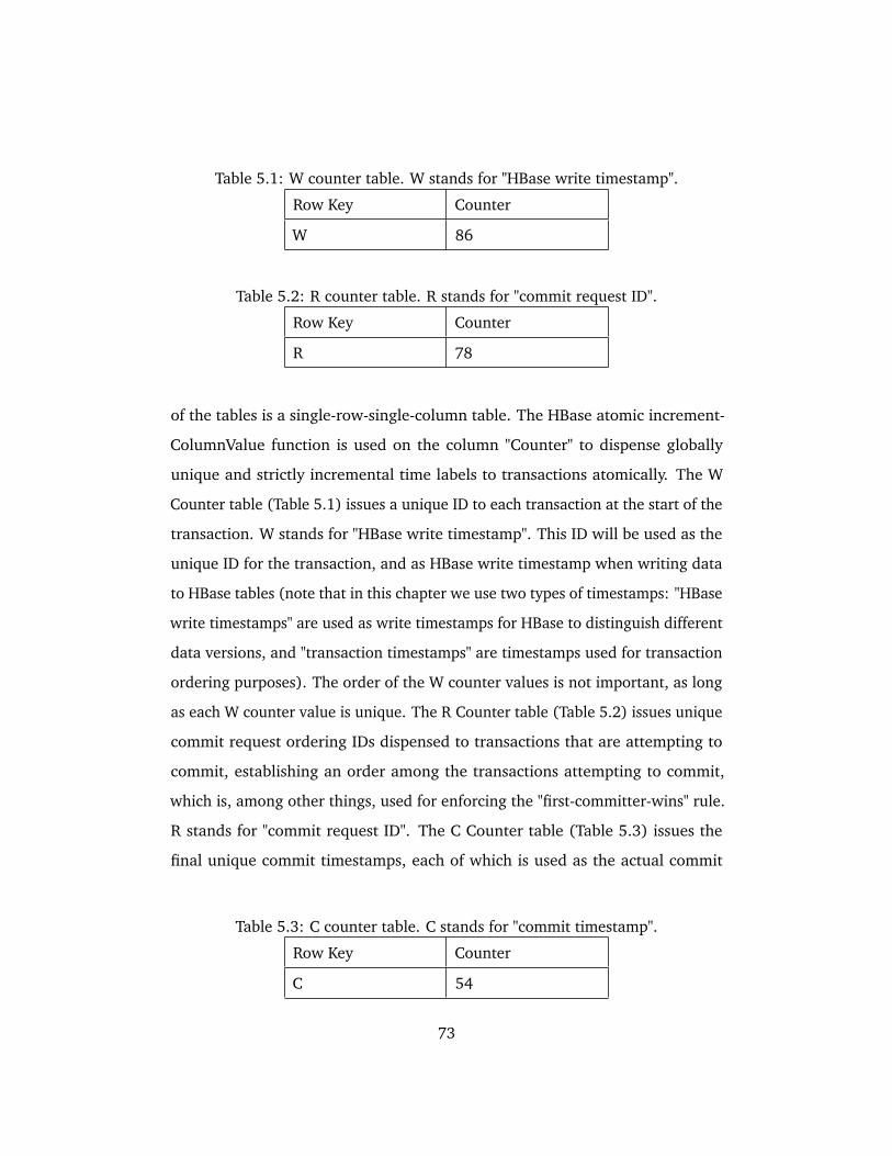
Table 5.1: W counter table. W stands for "HBase write timestamp".

Row Key Counter

W 86

Table 5.2: R counter table. R stands for "commit request ID".

Row Key Counter

R 78

of the tables is a single-row-single-column table. The HBase atomic increment-

ColumnValue function is used on the column "Counter" to dispense globally

unique and strictly incremental time labels to transactions atomically. The W

Counter table (Table 5.1) issues a unique ID to each transaction at the start of the

transaction. W stands for "HBase write timestamp". This ID will be used as the

unique ID for the transaction, and as HBase write timestamp when writing data

to HBase tables (note that in this chapter we use two types of timestamps: "HBase

write timestamps" are used as write timestamps for HBase to distinguish different

data versions, and "transaction timestamps" are timestamps used for transaction

ordering purposes). The order of the W counter values is not important, as long

as each W counter value is unique. The R Counter table (Table 5.2) issues unique

commit request ordering IDs dispensed to transactions that are attempting to

commit, establishing an order among the transactions attempting to commit,

which is, among other things, used for enforcing the "first-committer-wins" rule.

R stands for "commit request ID". The C Counter table (Table 5.3) issues the

final unique commit timestamps, each of which is used as the actual commit

Table 5.3: C counter table. C stands for "commit timestamp".

Row Key Counter

C 54

73

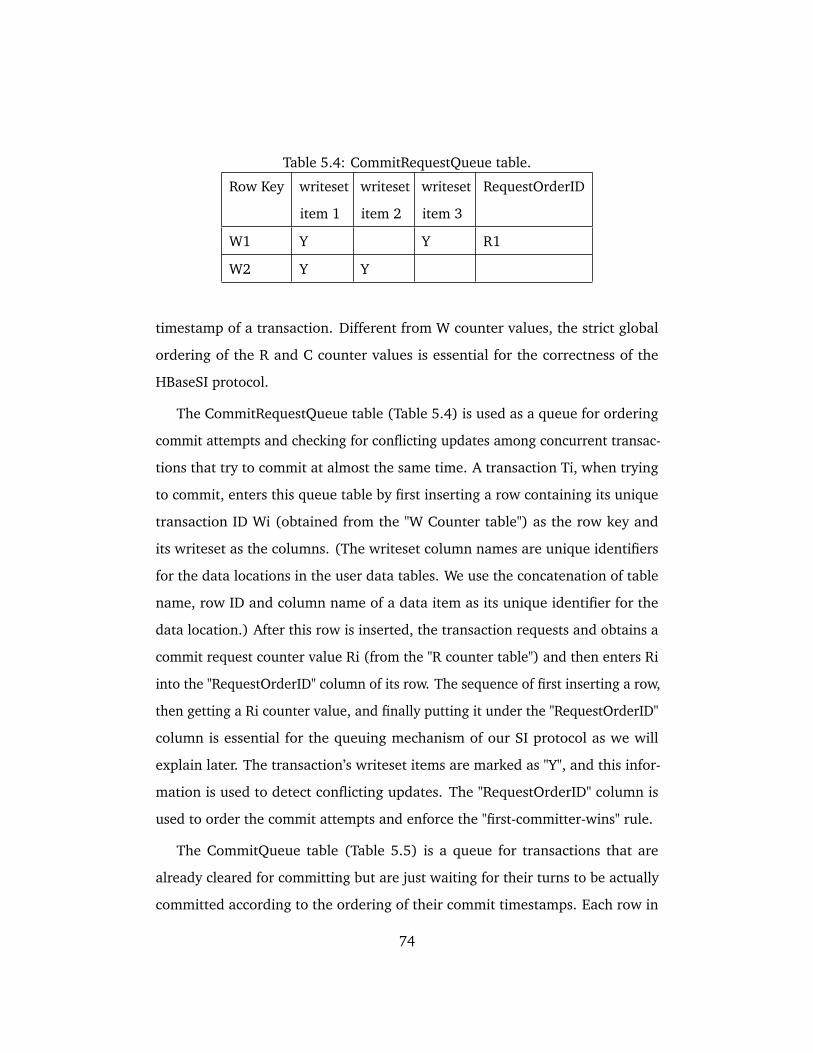
Table 5.4: CommitRequestQueue table.

Row Key writeset

item 1

writeset

item 2

writeset

item 3

RequestOrderID

W1 Y Y R1

W2 Y Y

timestamp of a transaction. Different from W counter values, the strict global

ordering of the R and C counter values is essential for the correctness of the

HBaseSI protocol.

The CommitRequestQueue table (Table 5.4) is used as a queue for ordering

commit attempts and checking for conflicting updates among concurrent transac-

tions that try to commit at almost the same time. A transaction Ti, when trying

to commit, enters this queue table by first inserting a row containing its unique

transaction ID Wi (obtained from the "W Counter table") as the row key and

its writeset as the columns. (The writeset column names are unique identifiers

for the data locations in the user data tables. We use the concatenation of table

name, row ID and column name of a data item as its unique identifier for the

data location.) After this row is inserted, the transaction requests and obtains a

commit request counter value Ri (from the "R counter table") and then enters Ri

into the "RequestOrderID" column of its row. The sequence of first inserting a row,

then getting a Ri counter value, and finally putting it under the "RequestOrderID"

column is essential for the queuing mechanism of our SI protocol as we will

explain later. The transaction’s writeset items are marked as "Y", and this infor-

mation is used to detect conflicting updates. The "RequestOrderID" column is

used to order the commit attempts and enforce the "first-committer-wins" rule.

The CommitQueue table (Table 5.5) is a queue for transactions that are

already cleared for committing but are just waiting for their turns to be actually

committed according to the ordering of their commit timestamps. Each row in

74

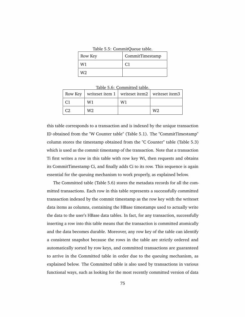
Table 5.5: CommitQueue table.

Row Key CommitTimestamp

W1 C1

W2

Table 5.6: Committed table.Row Key writeset item 1 writeset item2 writeset item3

C1 W1 W1

C2 W2 W2

this table corresponds to a transaction and is indexed by the unique transaction

ID obtained from the "W Counter table" (Table 5.1). The "CommitTimestamp"

column stores the timestamp obtained from the "C Counter" table (Table 5.3)

which is used as the commit timestamp of the transaction. Note that a transaction

Ti first writes a row in this table with row key Wi, then requests and obtains

its CommitTimestamp Ci, and finally adds Ci to its row. This sequence is again

essential for the queuing mechanism to work properly, as explained below.

The Committed table (Table 5.6) stores the metadata records for all the com-

mitted transactions. Each row in this table represents a successfully committed

transaction indexed by the commit timestamp as the row key with the writeset

data items as columns, containing the HBase timestamps used to actually write

the data to the user’s HBase data tables. In fact, for any transaction, successfully

inserting a row into this table means that the transaction is committed atomically

and the data becomes durable. Moreover, any row key of the table can identify

a consistent snapshot because the rows in the table are strictly ordered and

automatically sorted by row keys, and committed transactions are guaranteed

to arrive in the Committed table in order due to the queuing mechanism, as

explained below. The Committed table is also used by transactions in various

functional ways, such as looking for the most recently committed version of data

75

when reading, and checking for writeset conflicts at commit time against previ-

ously committed records. Note that HBase’s sparse column nature is crucial here

for efficiency: the table can contain many columns, but each column typically

contains only few elements, and can be scanned efficiently.

In HBaseSI, each transaction sees a consistent snapshot of all the data in

HBase user tables, identified by the start timestamp of the transaction. When a

transaction Ti starts, it first gets its start timestamp by reading the last row of the

Committed table at the time it starts, and uses the row key of that row Cj as the

start timestamp. So we have Si=Cj, and Ti will see all data committed by Tj, and

any transaction committed before Tj. Transaction Ti also obtains a unique ID Wi

from the "W Counter" table as its transaction ID. Then it performs reads/writes

based on the snapshot identified by the start timestamp. Data being read/written

are first saved in in-memory readset/writeset data structures so that repeated

reads can be efficiently served from memory, except for the first read/write of

a certain data item. In this way, it is guaranteed that the transaction reads its

own writes at all times. Writes are applied to the user data tables immediately

(speculatively) using the transaction ID Wi as the unique timestamp to write to

HBase (recall that a timestamp can be specified when writing data to HBase). At

commit time, the transaction puts itself into the CommitRequest table, may wait

for its turn if there are any conflicting commit attempts, then checks for conflicts

with committed transactions, and finally enters the CommitQueue table if it is

cleared to commit. It then waits for all the other concurrent transactions in the

CommitQueue table with smaller commit timestamp Ci to commit, and finally

commits by atomically inserting a simple record row into the Committed table to

make its writes durable. The pseudocode of the protocol is provided in Listing

5.1.

It is important to understand in detail how HBaseSI handles distributed syn-

chronization among concurrent transactions concerning the global ordering of

76

transaction commit requests and commits. HBaseSI makes use of distributed

queues to manage transaction commits and to guarantee the "first-committer-

wins" rule, instead of using other traditional methods such as data locks or

consensus-based protocols. The benefit is simplicity in design and implementa-

tion. HBaseSI makes use of two queues, implemented as two HBase tables. One

is the CommitRequestQueue (Table 5.4); the other is the CommitQueue (Table

5.5). The protocol to ensure a correct sequence of entering and exiting a queue

is the same for the two queues and therefore we explain the protocol using one

queue, the CommitRequestQueue, as an example. Recall that when a transaction

Ti makes a request to start the commit process, it first inserts a row indexed

by its unique transaction ID Wi (obtained from the "W Counter table"), then

gets a commit request counter value Ri and puts it under the "RequestOrderID"

column of its row. The Ri value determines the order of Ti in the queue. This

sequence of operations is of essential importance to guarantee that no concurrent

transaction will leave the queue out of order, as we explain now. After transaction

Ti inserts counter value Ri into its row in the CommitRequestQueue table, it

reads all records in the table once. It then waits until all rows of transactions

Tj it has read obtain Rj values in the table. This is essential to allow the queue

to function based on the order of the R counter values: Ti is guaranteed to see

any transaction Tj still in the queue that may have Rj<Ri, even if Rj appears

in the table after Ri. This is so because Ti reads the table after it has obtained

Ri, and any Tj still in the queue that may have Rj<Ri is guaranteed to have its

row in the table at that time, because it inserted its row before requesting Rj.

Ti will not proceed to the commit process until all Tj with Rj<Ri have left the

queue, guaranteeing that transactions are processed in order and establishing

the "first-committer-wins" rule. Based on the strict sequence of transactions

entering the queue table, the protocol to ensure the ordering of exiting the queue

is shown in Listing 5.1: pseudocode line 49 to 69. The pseudocode contains

77

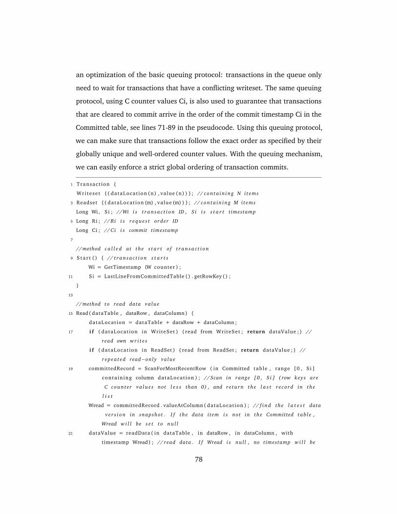
an optimization of the basic queuing protocol: transactions in the queue only

need to wait for transactions that have a conflicting writeset. The same queuing

protocol, using C counter values Ci, is also used to guarantee that transactions

that are cleared to commit arrive in the order of the commit timestamp Ci in the

Committed table, see lines 71-89 in the pseudocode. Using this queuing protocol,

we can make sure that transactions follow the exact order as specified by their

globally unique and well-ordered counter values. With the queuing mechanism,

we can easily enforce a strict global ordering of transaction commits.

1 Transac t ion

Wr i te se t ( dataLocat ion (n) , value (n) ) ; // con ta in ing N i t ems

3 Readset ( dataLocat ion (m) , value (m) ) ; // con ta in ing M i t ems

Long Wi , S i ; //Wi i s t r a n s a c t i o n ID , S i i s s t a r t t imestamp

5 Long Ri ; // Ri i s r e q u e s t order ID

Long Ci ; // Ci i s commit timestamp

7

// method c a l l e d at the s t a r t o f t r a n s a c t i o n

9 S t a r t () // t r a n s a c t i o n s t a r t s

Wi = GetTimestamp (W counter ) ;

11 Si = LastLineFromCommittedTable () . getRowKey () ;

13

// method to read data va lue

15 Read( dataTable , dataRow , dataColumn )

dataLocat ion = dataTable + dataRow + dataColumn ;

17 i f ( dataLocat ion in Wri teSet ) read from WriteSet ; return dataValue ; //

read own w r i t e s

i f ( dataLocat ion in ReadSet ) read from ReadSet ; return dataValue ; //

r ep ea t ed read−only va lue

19 committedRecord = ScanForMostRecentRow ( in Committed tab le , range [0 , S i ]

conta in ing column dataLocat ion ) ; // Scan in range [0 , S i ] ( row keys are

C count e r v a l u e s not l e s s than 0) , and r e tu rn the l a s t r e c o rd in the

l i s t

Wread = committedRecord . valueAtColumn ( dataLocat ion ) ; // f i n d the l a t e s t data

v e r s i o n in snapshot . I f the data i tem i s not in the Committed tab l e ,

Wread w i l l be s e t to n u l l

21 dataValue = readData ( in dataTable , in dataRow , in dataColumn , with

timestamp Wread) ; // read data . I f Wread i s nu l l , no timestamp w i l l be

78

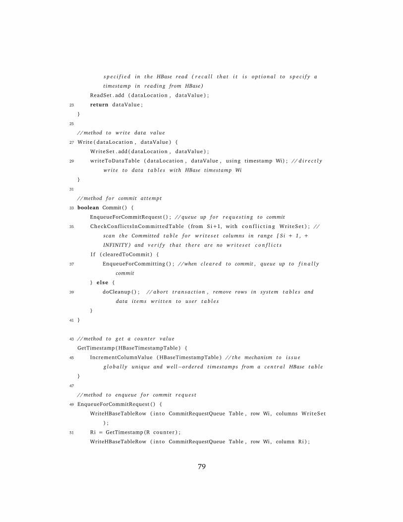
s p e c i f i e d in the HBase read ( r e c a l l t ha t i t i s o p t i o n a l to s p e c i f y a

timestamp in read ing from HBase )

ReadSet . add ( dataLocat ion , dataValue ) ;

23 return dataValue ;

25

// method to w r i t e data va lue

27 Write ( dataLocat ion , dataValue )

Wri teSet . add( dataLocat ion , dataValue ) ;

29 writeToDataTable ( dataLocat ion , dataValue , us ing timestamp Wi) ; // d i r e c t l y

w r i t e to data t a b l e s with HBase timestamp Wi

31

// method f o r commit at tempt

33 boolean Commit ()

EnqueueForCommitRequest () ; // queue up f o r r e q u e s t i n g to commit

35 CheckConf l ic ts InCommittedTable ( from Si +1, with c o n f l i c t i n g Wri teSet ) ; //

scan the Committed t a b l e f o r w r i t e s e t columns in range [ S i + 1 , +

INFINITY ) and v e r i f y tha t t h e r e are no w r i t e s e t c o n f l i c t s

I f ( clearedToCommit )

37 EnqueueForCommitting () ; //when c l e a r e d to commit , queue up to f i n a l l y

commit

else

39 doCleanup () ; // abor t t r a n s a c t i o n , remove rows in sys tem t a b l e s and

data i t ems w r i t t e n to u s e r t a b l e s

41

43 // method to g e t a coun t e r va lue

GetTimestamp ( HBaseTimestampTable )

45 IncrementColumnValue ( HBaseTimestampTable ) // the mechanism to i s s u e

g l o b a l l y unique and wel l−ordered t imestamps from a c e n t r a l HBase t a b l e

47

// method to enqueue f o r commit r e q u e s t

49 EnqueueForCommitRequest ()

WriteHBaseTableRow ( in to CommitRequestQueue Table , row Wi , columns WriteSet

) ;

51 Ri = GetTimestamp (R counter ) ;

WriteHBaseTableRow ( in to CommitRequestQueue Table , row Wi , column Ri ) ;

79

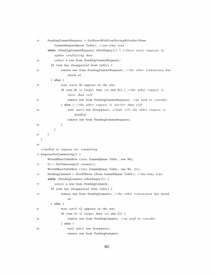
53 PendingCommitRequests = GetRowsWithConf l ic t ingWriteSet (From

CommitRequestQueue Table ) ; // one−t ime scan

while ( PendingCommitRequests . isNotEmpty () ) // t h e r e e x i s t r e q u e s t s to

update c o n f l i c t i n g data

55 s e l e c t a row from PendingCommitRequests ;

i f (row has disappeared from t a b l e )

57 remove row from PendingCommitRequests ; // the o the r t r a n s a c t i o n has

moved on

else

59 wait u n t i l Ri appears in the row ;

i f (row . Ri i s l a r g e r than i t s own Ri ) // the o the r r e q u e s t i s

l a t e r than s e l f

61 remove row from PendingCommitRequests ; //no need to c o n s i d e r

else // the o the r r e q u e s t i s e a r l i e r than s e l f

63 wait u n t i l row disappears ; // wait t i l l the o the r r e q u e s t i s

handled

remove row from PendingCommitRequests ;

65

67

69

// method to enqueue f o r committ ing

71 EnqueueForCommitting ()

WriteHBaseTableRow ( in to CommitQueue Table , row Wi) ;

73 Ci = GetTimestamp (C counter ) ;

WriteHBaseTableRow ( in to CommitQueue Table , row Wi , Ci ) ;

75 PendingCommits = GetAllRows (From CommitQueue Table ) ; // one−t ime scan

while ( PendingCommits . isNotEmpty () )

77 s e l e c t a row from PendingCommits ;

i f (row has disappeared from t a b l e )

79 remove row from PendingCommits ; // the o the r t r a n s a c t i o n has moved

on

else

81 wait u n t i l Ci appears in the row ;

i f (row . Ci i s l a r g e r than i t s own Ci )

83 remove row from PendingCommits ; //no need to c o n s i d e r

else

85 wait u n t i l row disappears ;

remove row from PendingCommits ;

80

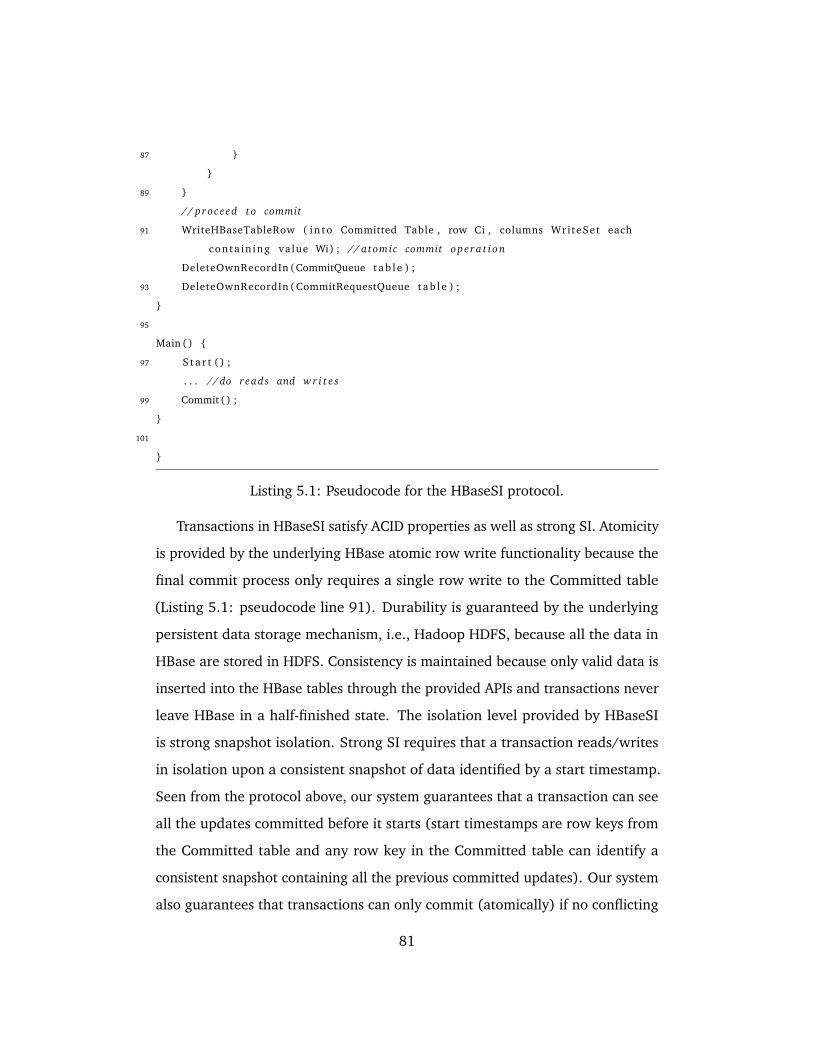
87

89

// proceed to commit

91 WriteHBaseTableRow ( in to Committed Table , row Ci , columns WriteSet each

conta in ing value Wi) ; // atomic commit ope ra t i on

DeleteOwnRecordIn (CommitQueue t a b l e ) ;

93 DeleteOwnRecordIn ( CommitRequestQueue t a b l e ) ;

95

Main ()

97 S t a r t () ;

. . . //do reads and w r i t e s

99 Commit () ;

101

Listing 5.1: Pseudocode for the HBaseSI protocol.

Transactions in HBaseSI satisfy ACID properties as well as strong SI. Atomicity

is provided by the underlying HBase atomic row write functionality because the

final commit process only requires a single row write to the Committed table

(Listing 5.1: pseudocode line 91). Durability is guaranteed by the underlying

persistent data storage mechanism, i.e., Hadoop HDFS, because all the data in

HBase are stored in HDFS. Consistency is maintained because only valid data is

inserted into the HBase tables through the provided APIs and transactions never

leave HBase in a half-finished state. The isolation level provided by HBaseSI

is strong snapshot isolation. Strong SI requires that a transaction reads/writes

in isolation upon a consistent snapshot of data identified by a start timestamp.

Seen from the protocol above, our system guarantees that a transaction can see

all the updates committed before it starts (start timestamps are row keys from

the Committed table and any row key in the Committed table can identify a

consistent snapshot containing all the previous committed updates). Our system

also guarantees that transactions can only commit (atomically) if no conflicting

81

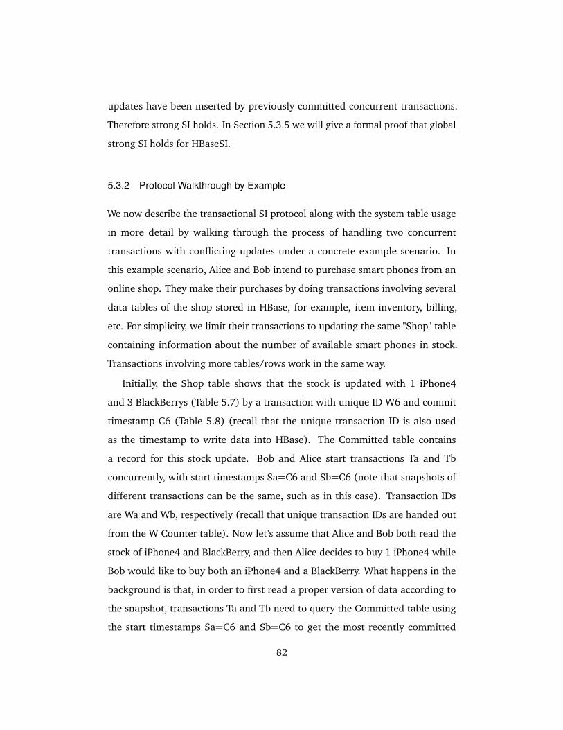
updates have been inserted by previously committed concurrent transactions.

Therefore strong SI holds. In Section 5.3.5 we will give a formal proof that global

strong SI holds for HBaseSI.

5.3.2 Protocol Walkthrough by Example

We now describe the transactional SI protocol along with the system table usage

in more detail by walking through the process of handling two concurrent

transactions with conflicting updates under a concrete example scenario. In

this example scenario, Alice and Bob intend to purchase smart phones from an

online shop. They make their purchases by doing transactions involving several

data tables of the shop stored in HBase, for example, item inventory, billing,

etc. For simplicity, we limit their transactions to updating the same "Shop" table

containing information about the number of available smart phones in stock.

Transactions involving more tables/rows work in the same way.

Initially, the Shop table shows that the stock is updated with 1 iPhone4

and 3 BlackBerrys (Table 5.7) by a transaction with unique ID W6 and commit

timestamp C6 (Table 5.8) (recall that the unique transaction ID is also used

as the timestamp to write data into HBase). The Committed table contains

a record for this stock update. Bob and Alice start transactions Ta and Tb

concurrently, with start timestamps Sa=C6 and Sb=C6 (note that snapshots of

different transactions can be the same, such as in this case). Transaction IDs

are Wa and Wb, respectively (recall that unique transaction IDs are handed out

from the W Counter table). Now let’s assume that Alice and Bob both read the

stock of iPhone4 and BlackBerry, and then Alice decides to buy 1 iPhone4 while

Bob would like to buy both an iPhone4 and a BlackBerry. What happens in the

background is that, in order to first read a proper version of data according to

the snapshot, transactions Ta and Tb need to query the Committed table using

the start timestamps Sa=C6 and Sb=C6 to get the most recently committed

82

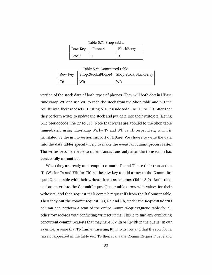
Table 5.7: Shop table.

Row Key iPhone4 BlackBerry

Stock 1 3

Table 5.8: Committed table.Row Key Shop:Stock:iPhone4 Shop:Stock:BlackBerry

C6 W6 W6

version of the stock data of both types of phones. They will both obtain HBase

timestamp W6 and use W6 to read the stock from the Shop table and put the

results into their readsets. (Listing 5.1: pseudocode line 15 to 23) After that

they perform writes to update the stock and put data into their writesets (Listing

5.1: pseudocode line 27 to 31). Note that writes are applied to the Shop table

immediately using timestamp Wa by Ta and Wb by Tb respectively, which is

facilitated by the multi-version support of HBase. We choose to write the data

into the data tables speculatively to make the eventual commit process faster.

The writes become visible to other transactions only after the transaction has

successfully committed.

When they are ready to attempt to commit, Ta and Tb use their transaction

ID (Wa for Ta and Wb for Tb) as the row key to add a row to the CommitRe-

questQueue table with their writeset items as columns (Table 5.9). Both trans-

actions enter into the CommitRequestQueue table a row with values for their

writesets, and then request their commit request ID from the R Counter table.

Then they put the commit request IDs, Ra and Rb, under the RequestOrderID

column and perform a scan of the entire CommitRequestQueue table for all

other row records with conflicting writeset items. This is to find any conflicting

concurrent commit requests that may have Rj<Ra or Rj<Rb in the queue. In our

example, assume that Tb finishes inserting Rb into its row and that the row for Ta

has not appeared in the table yet. Tb then scans the CommitRequestQueue and

83

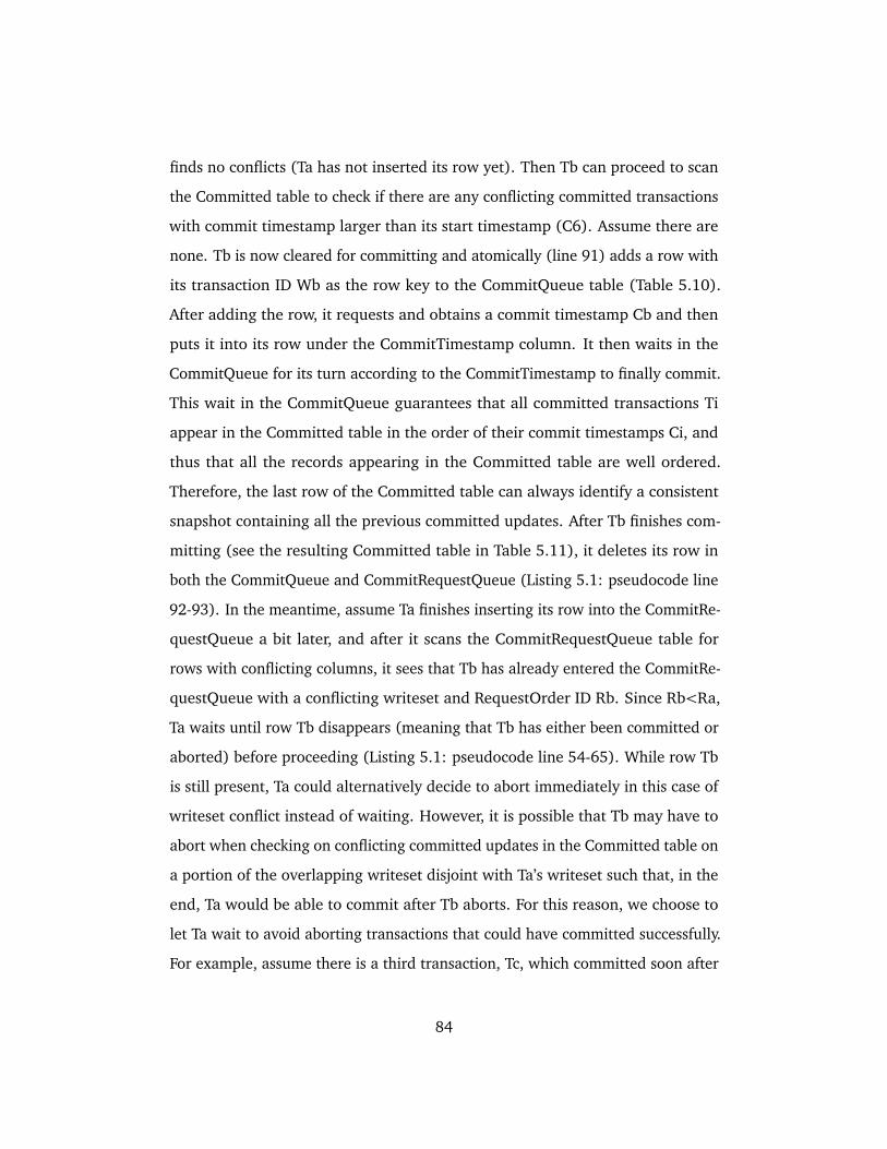
finds no conflicts (Ta has not inserted its row yet). Then Tb can proceed to scan

the Committed table to check if there are any conflicting committed transactions

with commit timestamp larger than its start timestamp (C6). Assume there are

none. Tb is now cleared for committing and atomically (line 91) adds a row with

its transaction ID Wb as the row key to the CommitQueue table (Table 5.10).

After adding the row, it requests and obtains a commit timestamp Cb and then

puts it into its row under the CommitTimestamp column. It then waits in the

CommitQueue for its turn according to the CommitTimestamp to finally commit.

This wait in the CommitQueue guarantees that all committed transactions Ti

appear in the Committed table in the order of their commit timestamps Ci, and

thus that all the records appearing in the Committed table are well ordered.

Therefore, the last row of the Committed table can always identify a consistent

snapshot containing all the previous committed updates. After Tb finishes com-

mitting (see the resulting Committed table in Table 5.11), it deletes its row in

both the CommitQueue and CommitRequestQueue (Listing 5.1: pseudocode line

92-93). In the meantime, assume Ta finishes inserting its row into the CommitRe-

questQueue a bit later, and after it scans the CommitRequestQueue table for

rows with conflicting columns, it sees that Tb has already entered the CommitRe-

questQueue with a conflicting writeset and RequestOrder ID Rb. Since Rb<Ra,

Ta waits until row Tb disappears (meaning that Tb has either been committed or

aborted) before proceeding (Listing 5.1: pseudocode line 54-65). While row Tb

is still present, Ta could alternatively decide to abort immediately in this case of

writeset conflict instead of waiting. However, it is possible that Tb may have to

abort when checking on conflicting committed updates in the Committed table on

a portion of the overlapping writeset disjoint with Ta’s writeset such that, in the

end, Ta would be able to commit after Tb aborts. For this reason, we choose to

let Ta wait to avoid aborting transactions that could have committed successfully.

For example, assume there is a third transaction, Tc, which committed soon after

84

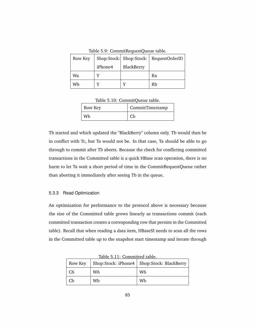
Table 5.9: CommitRequestQueue table.

Row Key Shop:Stock:

iPhone4

Shop:Stock:

BlackBerry

RequestOrderID

Wa Y Ra

Wb Y Y Rb

Table 5.10: CommitQueue table.

Row Key CommitTimestamp

Wb Cb

Tb started and which updated the "BlackBerry" column only. Tb would then be

in conflict with Tc, but Ta would not be. In that case, Ta should be able to go

through to commit after Tb aborts. Because the check for conflicting committed

transactions in the Committed table is a quick HBase scan operation, there is no

harm to let Ta wait a short period of time in the CommitRequestQueue rather

than aborting it immediately after seeing Tb in the queue.

5.3.3 Read Optimization

An optimization for performance to the protocol above is necessary because

the size of the Committed table grows linearly as transactions commit (each

committed transaction creates a corresponding row that persists in the Committed

table). Recall that when reading a data item, HBaseSI needs to scan all the rows

in the Committed table up to the snapshot start timestamp and iterate through

Table 5.11: Committed table.Row Key Shop:Stock: iPhone4 Shop:Stock: BlackBerry

C6 W6 W6

Cb Wb Wb

85

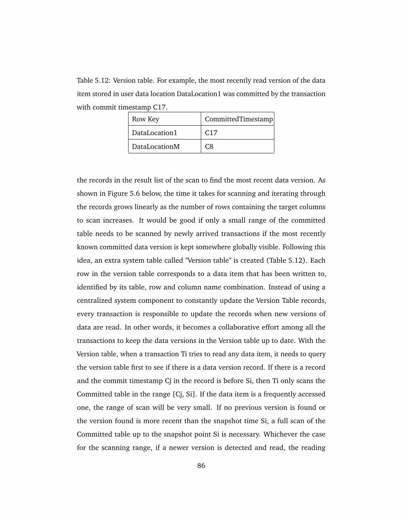
Table 5.12: Version table. For example, the most recently read version of the data

item stored in user data location DataLocation1 was committed by the transaction

with commit timestamp C17.

Row Key CommittedTimestamp

DataLocation1 C17

DataLocationM C8

the records in the result list of the scan to find the most recent data version. As

shown in Figure 5.6 below, the time it takes for scanning and iterating through

the records grows linearly as the number of rows containing the target columns

to scan increases. It would be good if only a small range of the committed

table needs to be scanned by newly arrived transactions if the most recently

known committed data version is kept somewhere globally visible. Following this

idea, an extra system table called "Version table" is created (Table 5.12). Each

row in the version table corresponds to a data item that has been written to,

identified by its table, row and column name combination. Instead of using a

centralized system component to constantly update the Version Table records,

every transaction is responsible to update the records when new versions of

data are read. In other words, it becomes a collaborative effort among all the

transactions to keep the data versions in the Version table up to date. With the

Version table, when a transaction Ti tries to read any data item, it needs to query

the version table first to see if there is a data version record. If there is a record

and the commit timestamp Cj in the record is before Si, then Ti only scans the

Committed table in the range [Cj, Si]. If the data item is a frequently accessed

one, the range of scan will be very small. If no previous version is found or

the version found is more recent than the snapshot time Si, a full scan of the

Committed table up to the snapshot point Si is necessary. Whichever the case

for the scanning range, if a newer version is detected and read, the reading

86

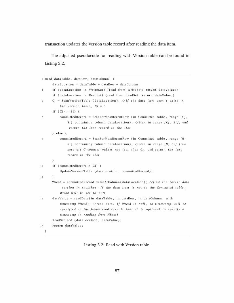
transaction updates the Version table record after reading the data item.

The adjusted pseudocode for reading with Version table can be found in

Listing 5.2.

1 Read( dataTable , dataRow , dataColumn )

dataLocat ion = dataTable + dataRow + dataColumn ;

3 i f ( dataLocat ion in Wri teSet ) read from WriteSet ; return dataValue ;

i f ( dataLocat ion in ReadSet ) read from ReadSet ; return dataValue ;

5 Cj = ScanVers ionTable ( dataLocat ion ) ; // i f the data i tem doen ’ t e x i s t in

the Ve r s i on tab l e , Cj = 0

i f ( Cj <= Si )

7 committedRecord = ScanForMostRecentRow ( in Committed tab le , range [ Cj ,

S i ] conta in ing column dataLocat ion ) ; // Scan in range [ Cj , S i ] , and

r e tu rn the l a s t r e c o rd in the l i s t

else

9 committedRecord = ScanForMostRecentRow ( in Committed tab le , range [0 ,

S i ] conta in ing column dataLocat ion ) ; // Scan in range [0 , S i ] ( row

keys are C count e r v a l u e s not l e s s than 0) , and r e tu rn the l a s t

r e c o rd in the l i s t

11 i f ( committedRecord > Cj )

UpdateVersionTable ( dataLocat ion , committedRecord ) ;

13

Wread = committedRecord . valueAtColumn ( dataLocat ion ) ; // f i n d the l a t e s t data

v e r s i o n in snapshot . I f the data i tem i s not in the Committed tab l e ,

Wread w i l l be s e t to n u l l

15 dataValue = readData ( in dataTable , in dataRow , in dataColumn , with

timestamp Wread) ; // read data . I f Wread i s nu l l , no timestamp w i l l be

s p e c i f i e d in the HBase read ( r e c a l l t ha t i t i s o p t i o n a l to s p e c i f y a

timestamp in read ing from HBase )

ReadSet . add ( dataLocat ion , dataValue ) ;

17 return dataValue ;

Listing 5.2: Read with Version table.

87

5.3.4 Handling Stragglers

In the protocol above, a transaction needs to wait in two queues, the CommitRe-

questQueue and the CommitQueue. Due to many possible failure conditions,

transactions could stay in waiting forever if one or more of the previously sub-

mitted transactions get stuck in the commit process and never delete their

corresponding rows in the above two queue tables. We call those transactions

that do not terminate properly in a timely manner "stragglers". Detecting and

handling such stragglers is difficult due to the large variety of possible failures.

Also, false positives can be problematic (treating some slow transactions as dead

whereas they may come back to an active state at some undetermined time in

the future). Measures must be taken to not only prevent such stragglers from

hampering the other active transactions, but also to avoid any potential data

inconsistency issues caused by re-appearing transactions that had been deemed

to be dead.

HBaseSI handles stragglers by adding a timeout mechanism to the waiting

transactions. More specifically, the waiting transactions can kill and remove

straggling/failed transactions from the CommitRequestQueue or CommitQueue

based on the clock of the waiting transaction if a preconfigured timeout threshold

is reached. A problem associated with this method is that a straggler may come

back to life and try to resume the rest of its commit process after its records in

either queues are removed, which could cause data inconsistencies and incorrect

SI handling. The solution to this problem is to use the HBase atomic CheckAndPut

method on two rows at once in the Committed table when doing the final commit

rather than only using a simple atomic row write operation on one row. The

difference between CheckAndPut and simple row write is that the former method

guarantees an atomic chain of two operations involving checking a row and

writing to a possibly different row in the same HBase table, whereas the latter

method only guarantees atomicity for a single row write operation. To use

88

the CheckAndPut method, we first add an extra row called "timeout" in the

Committed table (Table 5.13). When it starts, each transaction first marks the

column named after its unique transaction ID Wi (obtained from the W Counter

table) in the "timeout" row as "N", meaning that the transaction is not in timeout

by default (a non-empty initial value "N" must be set because the CheckAndPut

method does not work with empty column values). Later, in the commit process,

if a transaction is deemed a straggler, other transactions will put a "Y" under the

column named after the unique transaction ID of the straggler in the "timeout"

row, and then delete the corresponding records of the straggler in both the

CommitRequestQueue and the CommitQueue. (Note that the sequence of first

marking the straggler in the Committed table and only then deleting rows in the

two queues is essential to the correctness of the SI mechanism). When a healthy

transaction commits, it performs an atomic CheckAndPut: it checks for "N" in the

"timeout" row, and if the check is successful, it puts its row into the Committed

table. If the value under its corresponding column is still marked as "N", it can

indeed successfully insert its row into the Committed table; otherwise it knows it

has been marked as a straggler and should abort by deleting its records in both

the CommitRequestQueue and the CommitQueue tables, if those records still

exist. In this way, HBaseSI can make sure that no transaction can commit once

it is marked as a straggler. There is no problem if after a transaction commits

successfully by inserting a row into the Committed table, it fails to delete the

corresponding rows in the queues on time; those records will be removed by

waiting transactions after the timeout and SI is not compromised. Note that

for garbage cleaning purposes, after a transaction successfully commits, it can

remove the corresponding column value in the row "timeout".

89

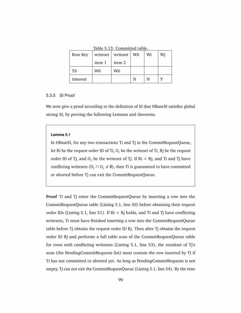
Table 5.13: Committed table.Row Key writeset

item 1

writeset

item 2

W6 Wi Wj

T6 W6 W6

timeout N N Y

5.3.5 SI Proof

We now give a proof according to the definition of SI that HBaseSI satisfies global

strong SI, by proving the following Lemmas and theorems.

Lemma 5.1

In HBaseSI, for any two transactions Ti and Tj in the CommitRequestQueue,

let Ri be the request order ID of Ti, Ωi be the writeset of Ti, Rj be the request

order ID of Tj, and Ω j be the writeset of Tj. If Ri < Rj, and Ti and Tj have

conflicting writesets (Ωi ∩ Ω j 6= ;), then Ti is guaranteed to have committed

or aborted before Tj can exit the CommitRequestQueue.

Proof Ti and Tj enter the CommitRequestQueue by inserting a row into the

CommitRequestQueue table (Listing 5.1, line 50) before obtaining their request

order IDs (Listing 5.1, line 51). If Ri < Rj holds, and Ti and Tj have conflicting

writesets, Ti must have finished inserting a row into the CommitRequestQueue

table before Tj obtains the request order ID Rj. Then after Tj obtains the request

order ID Rj and performs a full table scan of the CommitRequestQueue table

for rows with conflicting writesets (Listing 5.1, line 53), the resultset of Tj’s

scan (the PendingCommitRequests list) must contain the row inserted by Ti if

Ti has not committed or aborted yet. As long as PendingCommitRequests is not

empty, Tj can not exit the CommitRequestQueue (Listing 5.1, line 54). By the time

90

PendingCommitRequests is empty such that Tj can exit the CommitRequestQueue,

Ti is guaranteed to have committed or aborted because only in those two cases

will the row corresponding to Ti be deleted from the CommitRequestQueue

(having Ti’s row deleted from the CommitRequestQueue table because of the

straggler handling mechanism also means Ti has aborted). Therefore, the Lemma

holds.

Lemma 5.2

In HBaseSI, for any two transactions Ti and Tj in the CommitQueue, let Ci

be the commit timestamp of Ti and Cj be the commit timestamp of Tj. If Ci

< Cj, then Ti is guaranteed to have committed or aborted before Tj can exit

the CommitQueue.

Proof Ti and Tj enter the CommitQueue by inserting a row into the Com-

mitQueue table (Listing 5.1, line 72) before obtaining their commit timestamps

(Listing 5.1, line 73). If Ci < Cj holds, Ti must have finished inserting a row

into the CommitQueue table before Tj obtains the commit timestamp Cj. Then

after Tj obtains the commit timestamp Cj and performs a full table scan of the

CommitQueue table (Listing 5.1, line 75), the resultset of Tj’s scan (the Pend-

ingCommits list) must contain the row inserted by Ti if Ti has not committed

or aborted yet. As long as PendingCommits is not empty, Tj can not exit the

CommitQueue (Listing 5.1, line 76). By the time PendingCommits is empty such

that Tj can exit the CommitQueue, Ti is guaranteed to have committed or aborted

because only in those two cases will the row corresponding to Ti be deleted

from the CommitQueue (and having Ti’s row deleted from the CommitQueue

table because of the straggler handling mechanism also means Ti has aborted).

Therefore, the Lemma holds.

91

Lemma 5.3

In HBaseSI,

Part A: for any two transactions Ti and Tj, let Si be the start timestamp

of Ti and Cj be the commit timestamp of Tj. Then all updates made by the

committed transaction Tj which has the last Cj <= Si, as well as updates

made by committed transactions with commit timestamps smaller than Cj,

are visible to Ti when Ti starts;

Part B: all data items that have previously been written by transaction Ti

itself are visible to Ti.

Proof Part A: Let Ty be the transaction committed with commit timestamp Cy

which is the largest row key when Ti starts. Then Si = Cy. This means, Ty has

left the CommitQueue and committed by inserting a row into the Committed

table. We now prove by contradiction that all previously committed transactions

are also visible. Let Tx be some committed transaction with commit timestamp

Cx <= Si but assume the updates committed by Tx are not visible to Ti when Ti

starts. In other words, at the time Ti starts, the Committed table does not contain

a row with row key Cx. This would mean that Tx, with a commit timestamp Cx

< Cy (commit timestamps are unique according to the label issuing mechanism

of HBaseSI), has not yet committed. This contradicts Lemma 5.2. Therefore, Part

A holds.

Part B: All data items that have previously been written by transaction Ti itself

are stored in the writeset of Ti (Listing 5.1, line 28). The writeset of Ti is always

accessed first by read operations and will return the desired data value if the

data item is in the writeset (Listing 5.1, line 17). Therefore, Part B holds.

92

Lemma 5.4

In HBaseSI, for any two transactions Ti and Tj that are committed, let Si be

the start timestamp of Ti, Ci be the commit timestamp of Ti, Sj be the start

timestamp of Tj, and Cj be the commit timestamp of Tj. Then if (Si, Ci] ∩

(Sj, Cj] 6= ;, the writesets of Ti and Tj are guaranteed to be disjoint.

Proof We prove by contradiction as follows. Assume that Ti and Tj have conflict-

ing writesets and are both committed. Let Ri be the request order ID of Ti, and Rj

be the request order ID of Tj. Without loss of generality, let Ri < Rj (request order

IDs are unique and strictly ordered). According to Lemma 5.1, Ti is guaranteed

to have committed before Tj can exit the CommitRequestQueue. Then we have

Sj < Ci < Cj. Here, Sj < Ci must hold because otherwise (Si, Ci] ∩ (Sj, Cj] = ;,

and commit timestamps are unique and strictly ordered so that Ci < Cj holds.

After Ti commits, Tj may exit the CommitRequestQueue and performs a scan of

the Committed table in row range (Sj, ∞) (Listing 5.1, line 35). The resultset

must contain row Ci with writeset conflicting with Tj. Tj is then forced to abort

instead of being able to commit, which contradicts our assumption. Therefore,

the lemma holds.

Theorem 5.5

If Lemmas 5.3 and 5.4 are true, then HBaseSI satisfies global strong SI.

Proof We prove global strong SI according to the definition given in Section

5.2.1. For all the committed transactions in the transaction history, according to

Lemma 5.3, read operations in any transaction Ti see the data tables in the state

after the last commit before Si and can see the writes of Ti itself; according to

93

Lemma 5.4, concurrent transactions have disjoint writesets. Therefore, HBaseSI

satisfies global strong SI.

Theorem 5.6

The Version table optimization and straggler handling mechanism do not

affect the global strong SI guarantee of HBaseSI.

Proof The Version table optimization does not affect the upper bound of the scan

range (the upper bound equals the start timestamp Si of Ti, see Listing 5.2, line 7

and 9) in the Committed table for reads, nor does it affect the sequence of reading

from writeset first when reading a data item (Listing 5.2, line 3). Therefore,

Lemma 5.3 still holds. This optimization only concerns reads. Therefore, Lemma

5.4 still holds. According to Theorem 5.5, global strong SI still holds for HBaseSI.

The straggler handling mechanism deletes rows from the CommitRequestQueue

and CommitQueue table only after the "timeout" row has been marked in the

columns of the Committed table corresponding to the straggling transactions. The

atomicity of the HBase row write and checkAndPut operations guarantees that

once a row in the Committed table has received a "timeout" mark, the straggling

transaction cannot commit anymore, but can only abort. Therefore, Lemmas

5.1 and 5.2 still hold, and as a result, Lemmas 5.3 and 5.4 hold. According to

Theorem 5.5, global strong SI still holds for HBaseSI.

5.3.6 Discussion

In the previous sections, the detailed protocol of HBaseSI was elaborated with

an example scenario where Alice and Bob purchase smartphones. The Version

table optimization and straggler handling mechanism improve the efficiency

and robustness of the protocol. In this section, some further issues about the

94

HBaseSI design and usage are discussed. First, there is no roll back or roll

forward mechanism in HBaseSI and there is no explicit transaction log either.

It is interesting to ponder on how HBaseSI supports ACID transactions, even

in the face of failures, without those traditional mechanisms used in DBMSs.

In fact, this can all be attributed to two very important HBase properties. The

first one is that HBase stores many versions of data and allows reads/writes

of data using a specific timestamp. This HBase property makes it possible for

every concurrent transaction to write preliminary versions of data but only the

successfully committed transactions get to publish the write timestamps they

used in the Committed table for future reads. In other words, no roll back

is necessary because uncommitted data won’t be used in any case. The other

property is the atomicity of the HBase row write and CheckAndPut methods.

Using these atomic methods, HBase guarantees that once a row is inserted into

the Committed table successfully, it becomes durable and is guaranteed to survive

failures (media failure is handled by HDFS which stores data replicated across

distributed locations).

Second, we discuss some design choices that affect performance such as

scalability and disk usage. HBaseSI inherits many of the desirable properties of

HBase because it is only a client library and imposes little overhead concerning

system deployment. However, users need to be aware that in order to achieve

several design goals, HBaseSI sacrifices some performance. For example, four

important goals HBaseSI tries to achieve are: 1. global strong SI across table

boundaries; 2. non-intrusive to user data tables; 3. non-blocking start of transac-

tions with snapshots that are as fresh as possible (strong SI), and non-blocking

reads; 4. strict "first-committer-wins" rule without lost transactions (transactions

only abort when there is no chance they will be able to commit successfully).

In order to achieve goal 2, HBaseSI is designed to use a separate set of system

HBase tables for maintaining transactional metadata for all user tables instead

95

of creating extra columns in each separate user table, which inevitably creates

potential performance bottlenecks at the small number of global system tables.

HBaseSI is therefore not designed to provide scalability in terms of the number

of transactions per unit time, but its target is to provide scalability in terms of

cloud size and user data size. HBaseSI makes the final commit process as short as

possible and allows writes to insert preliminary data into the user data tables as

the transaction proceeds rather than waiting till the commit time to apply all the

updates (note that when a transaction aborts, it should remove its written items

from user tables), avoiding possible large waiting latency incurred by transactions

with large writesets to be applied at commit time. In essence, HBaseSI trades disk

space for high throughput in transaction commits. Additionally, it is important

that the number of data versions HBase table locations can hold is set sufficiently

high. For example, for data items that are likely to be updated concurrently by

many clients, the number of versions allowed should be set to some larger value

than default so that all the concurrent client writes can succeed. Furthermore,

since multiple versions of old committed data may accumulate (the uncommitted

data are already cleared by transactions when they abort), a dedicated garbage

cleaning mechanism should be created for optimizing disk usage, with a policy on

maximum transaction duration (such a policy is important to guarantee that the

data that gets garbage-cleaned is not needed by any long-running transactions in

their snapshots taken some time ago).

Third, we discuss the efficiency of having transactions wait in queues when

committing. Recall that in the HBaseSI protocol, update transactions first wait in

the CommitRequestQueue for the purpose of establishing an order in committing

transactions and guaranteeing the "first-committer-wins" rule, and then wait

in the CommitQueue after they are cleared for committing for the purpose of

guaranteeing a correct global sequence of commits so that each row in the

Committed table can identify a consistent snapshot of the data tables. This allows

96

new transactions to immediately obtain a start timestamp and start reading (non-

blocking reads). Note that the first wait is only for transactions with conflicting

writesets, but the second wait results in sequential processing of all concurrent

transactions, no matter whether the writesets are in conflict or not. Although

these two waits are essential for the commit queuing mechanism to work so that

global strong SI can be achieved, it may sometimes be more efficient to relax the

second wait to the extent that a transaction only waits for other transactions that

use the same set of user tables. This would require transactions to declare in

advance which groups of tables they use. This relaxation is reasonable in real-

world applications. More specifically, for example, online e-commerce sites need

to worry about the data consistency for a certain product in stock accessed by

concurrent buyers through the same online portal (which means calling the same

transactional routine concurrently). Those transactions shouldn’t be waiting for

the ones updating employee records or salaries in the back end. HBaseSI can be

very easily adapted to such extended usage scenarios to make transactions more

efficient in terms of minimizing unnecessary wait times in the CommitQueue. The

decision of whether to use the extended scheme would be at the users’ discretion.

Also, in this case users cannot be allowed to write to tables outside the set they

have declared. The benefit of using the extended scheme is a possible boost

in performance, especially in the face of a large number of concurrent update

requests.

Finally, we discuss the cost of adopting HBaseSI and the easiness of reverting

back to non-SI default HBase. Normally, once one starts to use HBaseSI, all the

read/write operations must be performed through the HBaseSI API rather than

the default HBase API. Otherwise, the most recently updated data versions will

not be maintained and used. Only through the HBaseSI API can a transaction

find the correct timestamp used in writing the most up-to-date data, or make its

committed updates accessible. This is because the timestamps used by HBaseSI

97

could be smaller than the default timestamps HBase uses when no explicit

timestamps are specified for reads/writes. However, it is very easy to write a

small tool to help restore the user data tables back to a state that users can use

their data tables in the default HBase manner. The tool only needs to write

the latest version of committed data to all the user data tables once, without

specifying timestamps (so that the HBase default timestamps are used). The tool

should also delete all the tables used by HBaseSI storing transactional metadata

to make sure that no transactions could use the outdated transactional metadata

leading to errors. The next time users want to use HBaseSI again, they can simply

re-initialize the HBase tables for holding transactional metadata and start using

HBaseSI without any required changes to existing user data.

5.4 Performance Evaluation on Amazon EC2

The general purpose of this performance evaluation section is to quantify the cost

of adopting the HBaseSI protocol in handling concurrent transactions. Therefore

tests are performed on each critical step of the HBaseSI protocol, with comparison

to the performance of bare-bones HBase when possible. Additionally, because

HBaseSI is the first system that achieves global strong SI on HBase, there are no

other similar systems to compare with for some of the properties. As a result, for

those properties, the tests serve the purpose of showing the users the expected

behavior of the system. Furthermore, as mentioned in Section 5.3 above, HBaseSI

uses a set of global system tables that facilitate non-blocking reads and a strict

"first-committer-wins" rule, but may become performance bottlenecks if accessed

by many concurrent transactions. The test results are thus expected to reflect the

system performance under varying loads.

We use 20 Amazon machines in total to perform the tests and we are aware

that performance variations may be observed in Amazon instances [40]. The

test results may be affected by this to some extent but should be sufficient for

98

proof-of-concept purposes. A high memory 64-bit linux instance with 15 GB

memory, 8 EC2 Compute Units (4 virtual cores with 2 EC2 Compute Units each)

and high I/O performance is used to host the Hadoop namenode, jobtracker

and the HBase master system component. Up to 19 other high CPU 64-bit linux

instances with 7 GB of memory, 20 EC2 Compute Units (8 virtual cores with 2.5

EC2 Compute Units each) and high I/O performance are used to host Hadoop

datanodes, HBase regionservers and run client transactions. The reason to choose

a high memory instance to be the master server is because of the observation that

under heavy loads from many concurrent clients, the mostly consumed resource

at the server is memory. For instances running client transactions, however, the

mostly consumed resource is CPU cycles, which is why the other 19 instances are

chosen to be high CPU instances so that multiple client transactions can be run

on each one of them. All these machines are in the same Amazon availability

zone so that the network conditions for each instance are assumed to be similar.

In the tests, each machine instance runs a single client program issuing

transactions if the total number of clients is less than 19. If the total number of

clients is more than 19, an equal number of concurrent clients are run at each

machine instance. For example, each machine instance can run 1, 2, or more

clients with the total number of transactions being 19, 38, etc. At each client,

transactions are issued consecutively one after another. In other words, a new

transaction will only be issued when the previous one has finished executing,

having either committed or aborted. Each transaction is executed for 3 times

and the performance measure for the corresponding transaction is calculated as

the average of the measures obtained from the 3 runs. We do this to average

out the short-term performance variance of the Amazon EC2, which is further

discussed at the end of this section. Additionally, we perform all the different

tests (described below) in a single large batch on the same virtual cluster, in

order to minimize the potential effects of long term performance variance (e.g.,

99

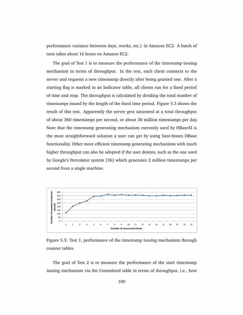
performance variance between days, weeks, etc.) in Amazon EC2. A batch of

tests takes about 16 hours on Amazon EC2.

The goal of Test 1 is to measure the performance of the timestamp issuing

mechanism in terms of throughput. In the test, each client connects to the

server and requests a new timestamp directly after being granted one. After a

starting flag is marked in an Indicator table, all clients run for a fixed period

of time and stop. The throughput is calculated by dividing the total number of

timestamps issued by the length of the fixed time period. Figure 5.3 shows the

result of this test. Apparently the server gets saturated at a total throughput

of about 360 timestamps per second, or about 30 million timestamps per day.

Note that the timestamp generating mechanism currently used by HBaseSI is

the most straightforward solution a user can get by using bare-bones HBase

functionality. Other more efficient timestamp generating mechanisms with much

higher throughput can also be adopted if the user desires, such as the one used

by Google’s Percolator system [36] which generates 2 million timestamps per

second from a single machine.

Figure 5.3: Test 1, performance of the timestamp issuing mechanism through

counter tables.

The goal of Test 2 is to measure the performance of the start timestamp

issuing mechanism via the Committed table in terms of throughput, i.e., how

100

many transactions can be allowed to start per second (in order for a transaction

to start, a start timestamp must be issued first) with an increasing number of

concurrent clients. Recall that the mechanism to obtain a start timestamp is

different from getting a unique counter value from one of the counter tables.

Instead, a transaction needs to read the last row of the Committed table at

the time it starts and use the row key as its start timestamp. In this test, the

clients all connect to the server first and then wait for a signal in the Indicator

table to start at the same time. During the test, a program is run at the EC2

instance running the HBase server inserting a new row to the Committed table

continuously, mimicking the real-world scenario where the Committed table

keeps growing in size because of newly committed transaction records. The

throughput is calculated in the same way as Test 1. Figure 5.4 shows the result

for Test 2. The throughput stabilizes at about 420 timestamps per second due to

server saturation, slightly higher than the result obtained from Test 1. The higher

performance is expected because in Test 1 an atomic function call to increment

a common column value is issued each time a counter value is to be obtained

by each concurrent client, potentially causing a blocking write conflict at the

HBase server, while in Test 2, only scanning the last row of the Committed table

is necessary. The performance is thus satisfactory to the extent that the start

timestamp mechanism is not the limiting bottleneck for starting new transactions

even if the mechanism requires that every transaction should read from the

Committed table at starting time.

The goal of Test 3 is to study the comparative performance of transactions

with SI that contain a set of read/write operations, against executions of the same

number of read/write operations with bare-bones HBase, for varying numbers

of operations per transaction. In the test, we run 1 client only, vary the number

of operations per transaction and measure the time spent on each read/write

operation. Additionally, in order to control the performance overhead associated

101

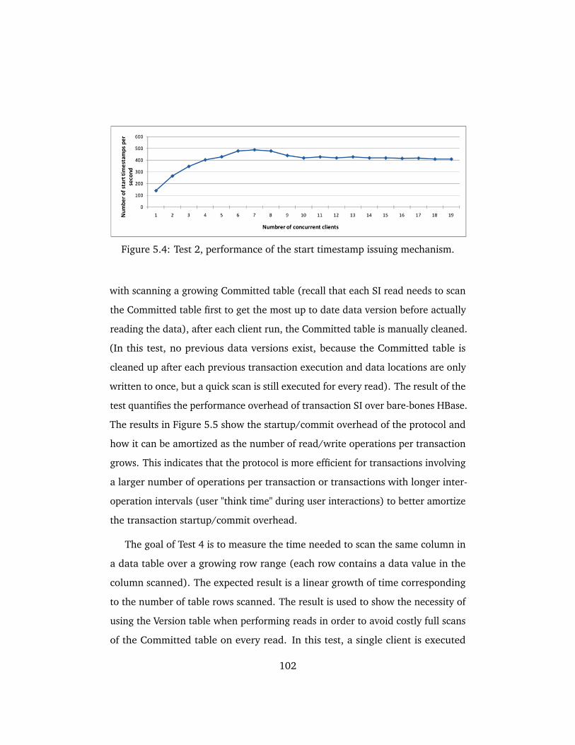
Figure 5.4: Test 2, performance of the start timestamp issuing mechanism.

with scanning a growing Committed table (recall that each SI read needs to scan

the Committed table first to get the most up to date data version before actually

reading the data), after each client run, the Committed table is manually cleaned.

(In this test, no previous data versions exist, because the Committed table is

cleaned up after each previous transaction execution and data locations are only

written to once, but a quick scan is still executed for every read). The result of the

test quantifies the performance overhead of transaction SI over bare-bones HBase.

The results in Figure 5.5 show the startup/commit overhead of the protocol and

how it can be amortized as the number of read/write operations per transaction

grows. This indicates that the protocol is more efficient for transactions involving

a larger number of operations per transaction or transactions with longer inter-

operation intervals (user "think time" during user interactions) to better amortize

the transaction startup/commit overhead.

The goal of Test 4 is to measure the time needed to scan the same column in

a data table over a growing row range (each row contains a data value in the

column scanned). The expected result is a linear growth of time corresponding

to the number of table rows scanned. The result is used to show the necessity of

using the Version table when performing reads in order to avoid costly full scans

of the Committed table on every read. In this test, a single client is executed

102

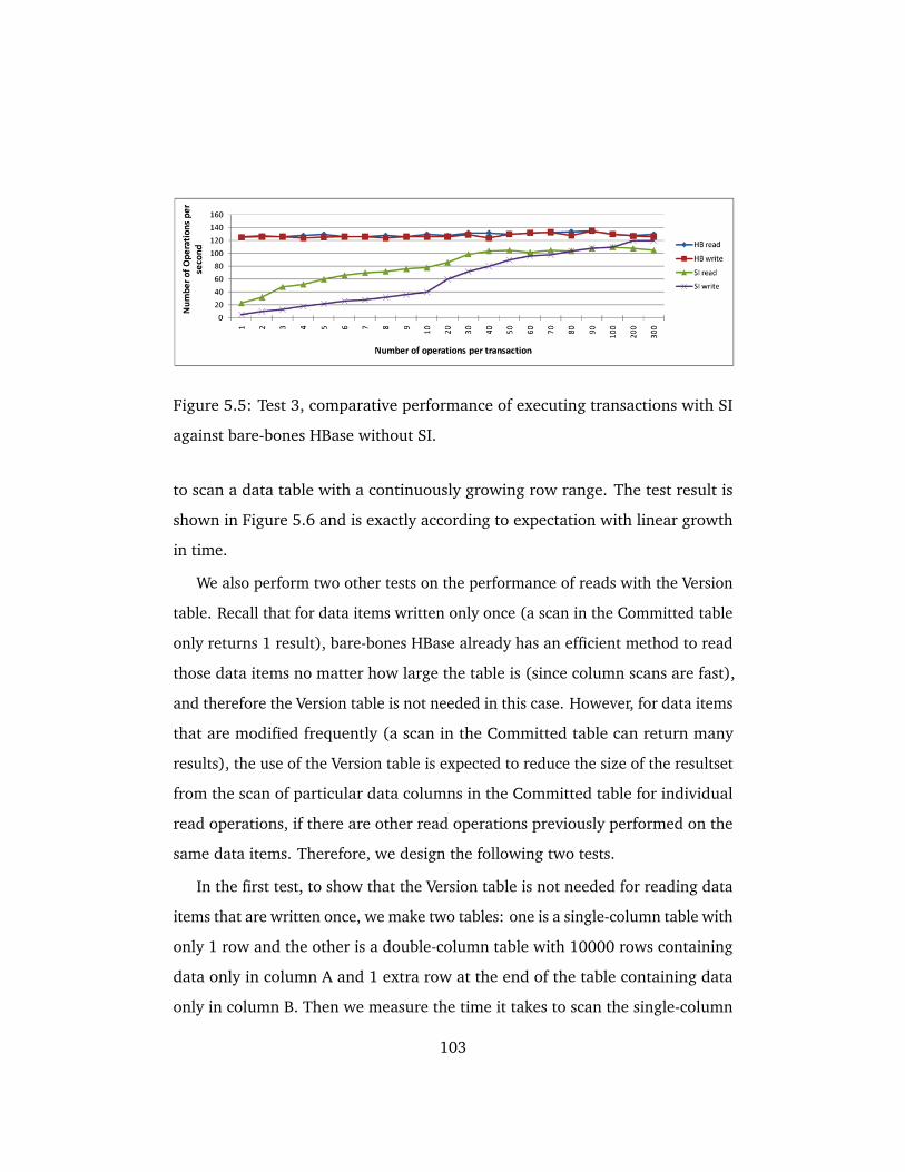
Figure 5.5: Test 3, comparative performance of executing transactions with SI

against bare-bones HBase without SI.

to scan a data table with a continuously growing row range. The test result is

shown in Figure 5.6 and is exactly according to expectation with linear growth

in time.

We also perform two other tests on the performance of reads with the Version

table. Recall that for data items written only once (a scan in the Committed table

only returns 1 result), bare-bones HBase already has an efficient method to read

those data items no matter how large the table is (since column scans are fast),

and therefore the Version table is not needed in this case. However, for data items

that are modified frequently (a scan in the Committed table can return many

results), the use of the Version table is expected to reduce the size of the resultset

from the scan of particular data columns in the Committed table for individual

read operations, if there are other read operations previously performed on the

same data items. Therefore, we design the following two tests.

In the first test, to show that the Version table is not needed for reading data

items that are written once, we make two tables: one is a single-column table with

only 1 row and the other is a double-column table with 10000 rows containing

data only in column A and 1 extra row at the end of the table containing data

only in column B. Then we measure the time it takes to scan the single-column

103

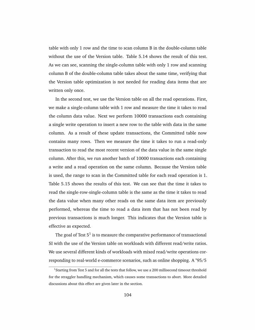
table with only 1 row and the time to scan column B in the double-column table

without the use of the Version table. Table 5.14 shows the result of this test.

As we can see, scanning the single-column table with only 1 row and scanning

column B of the double-column table takes about the same time, verifying that

the Version table optimization is not needed for reading data items that are

written only once.

In the second test, we use the Version table on all the read operations. First,

we make a single-column table with 1 row and measure the time it takes to read

the column data value. Next we perform 10000 transactions each containing

a single write operation to insert a new row to the table with data in the same

column. As a result of these update transactions, the Committed table now

contains many rows. Then we measure the time it takes to run a read-only

transaction to read the most recent version of the data value in the same single

column. After this, we run another batch of 10000 transactions each containing

a write and a read operation on the same column. Because the Version table

is used, the range to scan in the Committed table for each read operation is 1.

Table 5.15 shows the results of this test. We can see that the time it takes to

read the single-row-single-column table is the same as the time it takes to read

the data value when many other reads on the same data item are previously

performed, whereas the time to read a data item that has not been read by

previous transactions is much longer. This indicates that the Version table is

effective as expected.

The goal of Test 51 is to measure the comparative performance of transactional

SI with the use of the Version table on workloads with different read/write ratios.

We use several different kinds of workloads with mixed read/write operations cor-

responding to real-world e-commerce scenarios, such as online shopping. A "95/5

1Starting from Test 5 and for all the tests that follow, we use a 200 millisecond timeout threshold

for the straggler handling mechanism, which causes some transactions to abort. More detailed

discussions about this effect are given later in the section.

104

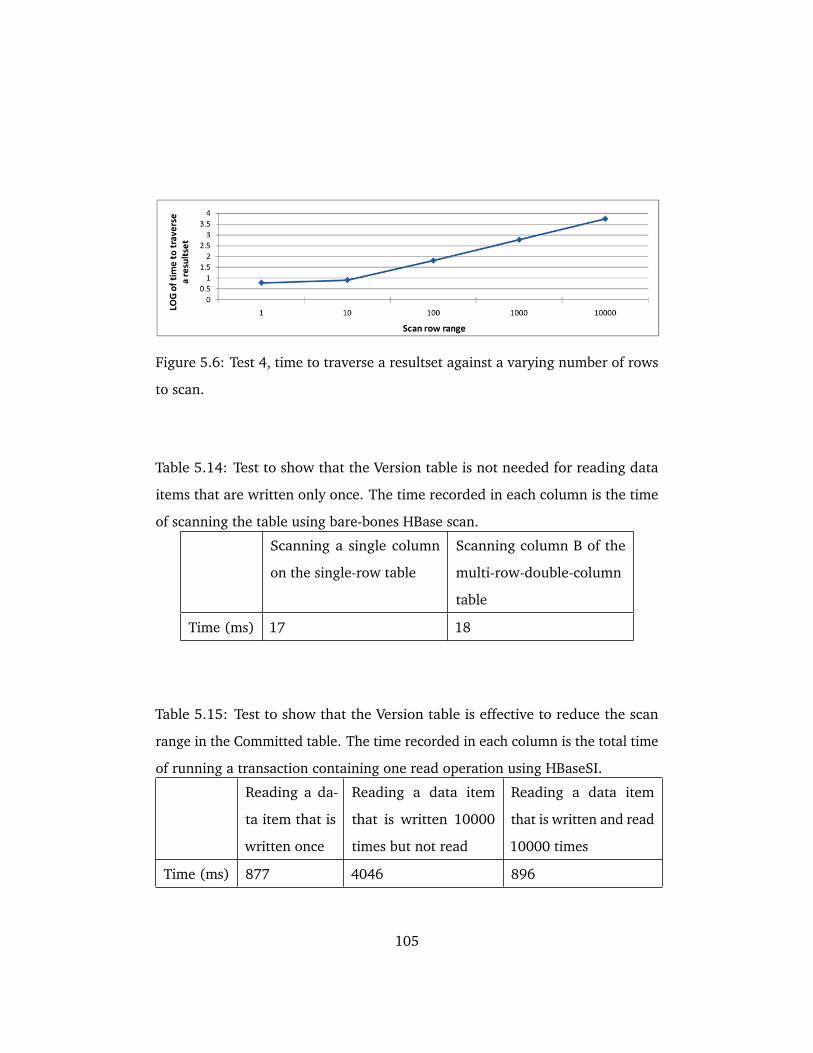
Figure 5.6: Test 4, time to traverse a resultset against a varying number of rows

to scan.

Table 5.14: Test to show that the Version table is not needed for reading data

items that are written only once. The time recorded in each column is the time

of scanning the table using bare-bones HBase scan.

Scanning a single column

on the single-row table

Scanning column B of the

multi-row-double-column

table

Time (ms) 17 18

Table 5.15: Test to show that the Version table is effective to reduce the scan

range in the Committed table. The time recorded in each column is the total time

of running a transaction containing one read operation using HBaseSI.

Reading a da-

ta item that is

written once

Reading a data item

that is written 10000

times but not read

Reading a data item

that is written and read

10000 times

Time (ms) 877 4046 896

105

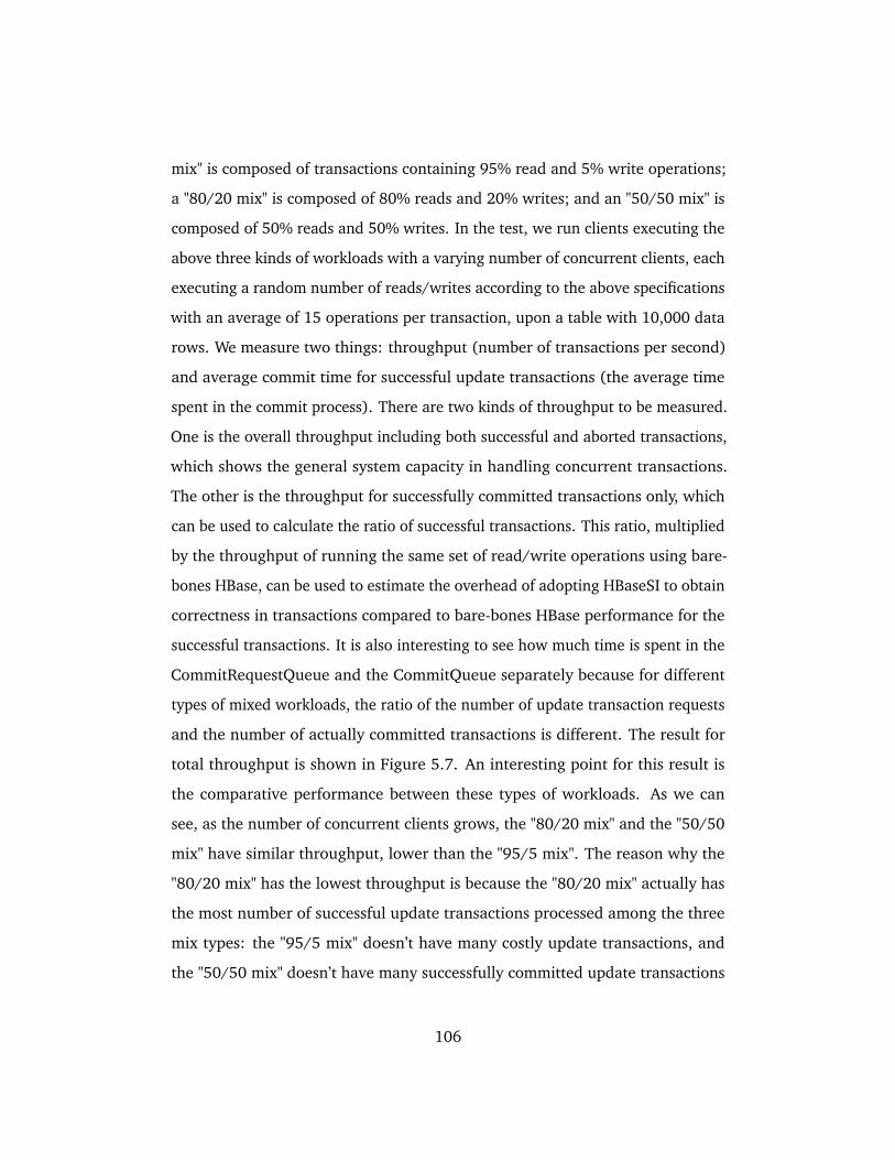
mix" is composed of transactions containing 95% read and 5% write operations;

a "80/20 mix" is composed of 80% reads and 20% writes; and an "50/50 mix" is

composed of 50% reads and 50% writes. In the test, we run clients executing the

above three kinds of workloads with a varying number of concurrent clients, each

executing a random number of reads/writes according to the above specifications

with an average of 15 operations per transaction, upon a table with 10,000 data

rows. We measure two things: throughput (number of transactions per second)

and average commit time for successful update transactions (the average time

spent in the commit process). There are two kinds of throughput to be measured.

One is the overall throughput including both successful and aborted transactions,

which shows the general system capacity in handling concurrent transactions.

The other is the throughput for successfully committed transactions only, which

can be used to calculate the ratio of successful transactions. This ratio, multiplied

by the throughput of running the same set of read/write operations using bare-

bones HBase, can be used to estimate the overhead of adopting HBaseSI to obtain

correctness in transactions compared to bare-bones HBase performance for the

successful transactions. It is also interesting to see how much time is spent in the

CommitRequestQueue and the CommitQueue separately because for different

types of mixed workloads, the ratio of the number of update transaction requests

and the number of actually committed transactions is different. The result for

total throughput is shown in Figure 5.7. An interesting point for this result is

the comparative performance between these types of workloads. As we can

see, as the number of concurrent clients grows, the "80/20 mix" and the "50/50

mix" have similar throughput, lower than the "95/5 mix". The reason why the

"80/20 mix" has the lowest throughput is because the "80/20 mix" actually has

the most number of successful update transactions processed among the three

mix types: the "95/5 mix" doesn’t have many costly update transactions, and

the "50/50 mix" doesn’t have many successfully committed update transactions

106

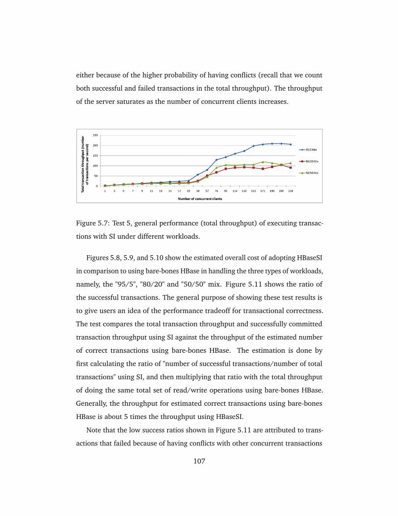
either because of the higher probability of having conflicts (recall that we count

both successful and failed transactions in the total throughput). The throughput

of the server saturates as the number of concurrent clients increases.

Figure 5.7: Test 5, general performance (total throughput) of executing transac-

tions with SI under different workloads.

Figures 5.8, 5.9, and 5.10 show the estimated overall cost of adopting HBaseSI

in comparison to using bare-bones HBase in handling the three types of workloads,

namely, the "95/5", "80/20" and "50/50" mix. Figure 5.11 shows the ratio of

the successful transactions. The general purpose of showing these test results is

to give users an idea of the performance tradeoff for transactional correctness.

The test compares the total transaction throughput and successfully committed

transaction throughput using SI against the throughput of the estimated number

of correct transactions using bare-bones HBase. The estimation is done by

first calculating the ratio of "number of successful transactions/number of total

transactions" using SI, and then multiplying that ratio with the total throughput

of doing the same total set of read/write operations using bare-bones HBase.

Generally, the throughput for estimated correct transactions using bare-bones

HBase is about 5 times the throughput using HBaseSI.

Note that the low success ratios shown in Figure 5.11 are attributed to trans-

actions that failed because of having conflicts with other concurrent transactions

107

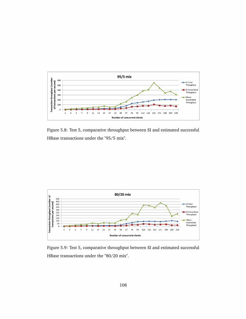
Figure 5.8: Test 5, comparative throughput between SI and estimated successful

HBase transactions under the "95/5 mix".

Figure 5.9: Test 5, comparative throughput between SI and estimated successful

HBase transactions under the "80/20 mix".

108

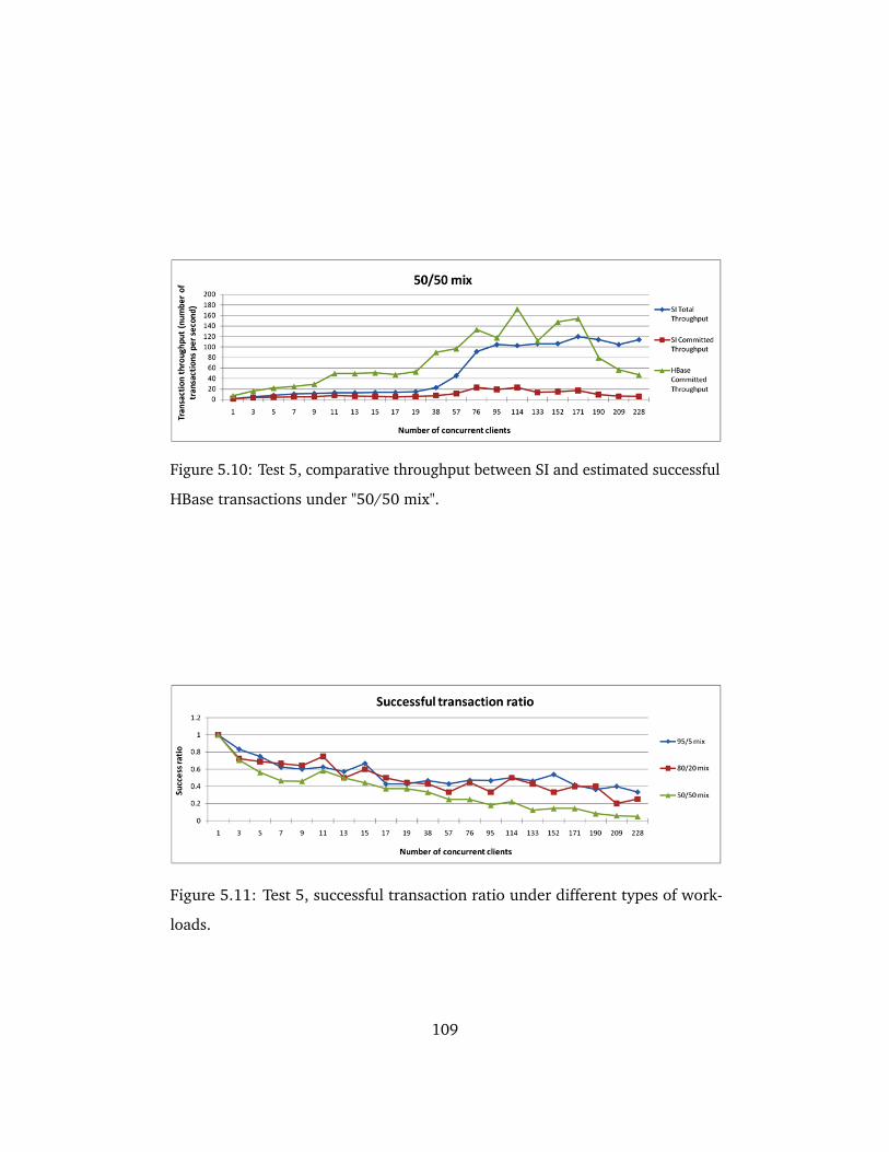
Figure 5.10: Test 5, comparative throughput between SI and estimated successful

HBase transactions under "50/50 mix".

Figure 5.11: Test 5, successful transaction ratio under different types of work-

loads.

109

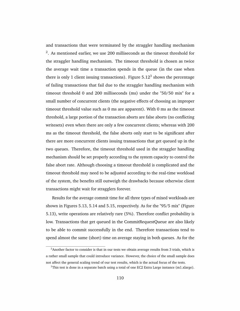
and transactions that were terminated by the straggler handling mechanism2. As mentioned earlier, we use 200 milliseconds as the timeout threshold for

the straggler handling mechanism. The timeout threshold is chosen as twice

the average wait time a transaction spends in the queue (in the case when

there is only 1 client issuing transactions). Figure 5.123 shows the percentage

of failing transactions that fail due to the straggler handling mechanism with

timeout threshold 0 and 200 milliseconds (ms) under the "50/50 mix" for a

small number of concurrent clients (the negative effects of choosing an improper

timeout threshold value such as 0 ms are apparent). With 0 ms as the timeout

threshold, a large portion of the transaction aborts are false aborts (no conflicting

writesets) even when there are only a few concurrent clients; whereas with 200

ms as the timeout threshold, the false aborts only start to be significant after

there are more concurrent clients issuing transactions that get queued up in the

two queues. Therefore, the timeout threshold used in the straggler handling

mechanism should be set properly according to the system capacity to control the

false abort rate. Although choosing a timeout threshold is complicated and the

timeout threshold may need to be adjusted according to the real-time workload

of the system, the benefits still outweigh the drawbacks because otherwise client

transactions might wait for stragglers forever.

Results for the average commit time for all three types of mixed workloads are

shown in Figures 5.13, 5.14 and 5.15, respectively. As for the "95/5 mix" (Figure

5.13), write operations are relatively rare (5%). Therefore conflict probability is

low. Transactions that get queued in the CommitRequestQueue are also likely

to be able to commit successfully in the end. Therefore transactions tend to

spend almost the same (short) time on average staying in both queues. As for the

2Another factor to consider is that in our tests we obtain average results from 3 trials, which is

a rather small sample that could introduce variance. However, the choice of the small sample does

not affect the general scaling trend of our test results, which is the actual focus of the tests.3This test is done in a separate batch using a total of one EC2 Extra Large instance (m1.xlarge).

110

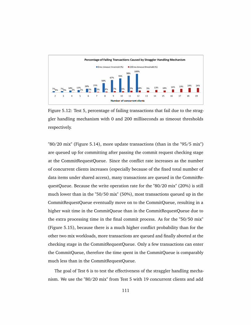
Figure 5.12: Test 5, percentage of failing transactions that fail due to the strag-

gler handling mechanism with 0 and 200 milliseconds as timeout thresholds

respectively.

"80/20 mix" (Figure 5.14), more update transactions (than in the "95/5 mix")

are queued up for committing after passing the commit request checking stage

at the CommitRequestQueue. Since the conflict rate increases as the number

of concurrent clients increases (especially because of the fixed total number of

data items under shared access), many transactions are queued in the CommitRe-

questQueue. Because the write operation rate for the "80/20 mix" (20%) is still

much lower than in the "50/50 mix" (50%), most transactions queued up in the

CommitRequestQueue eventually move on to the CommitQueue, resulting in a

higher wait time in the CommitQueue than in the CommitRequestQueue due to

the extra processing time in the final commit process. As for the "50/50 mix"

(Figure 5.15), because there is a much higher conflict probability than for the

other two mix workloads, more transactions are queued and finally aborted at the

checking stage in the CommitRequestQueue. Only a few transactions can enter

the CommitQueue, therefore the time spent in the CommitQueue is comparably

much less than in the CommitRequestQueue.

The goal of Test 6 is to test the effectiveness of the straggler handling mecha-

nism. We use the "80/20 mix" from Test 5 with 19 concurrent clients and add

111

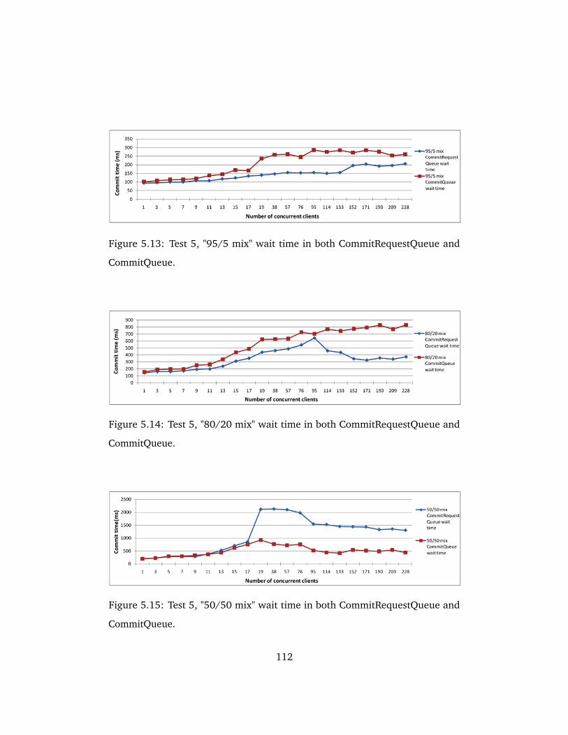
Figure 5.13: Test 5, "95/5 mix" wait time in both CommitRequestQueue and

CommitQueue.

Figure 5.14: Test 5, "80/20 mix" wait time in both CommitRequestQueue and

CommitQueue.

Figure 5.15: Test 5, "50/50 mix" wait time in both CommitRequestQueue and

CommitQueue.

112

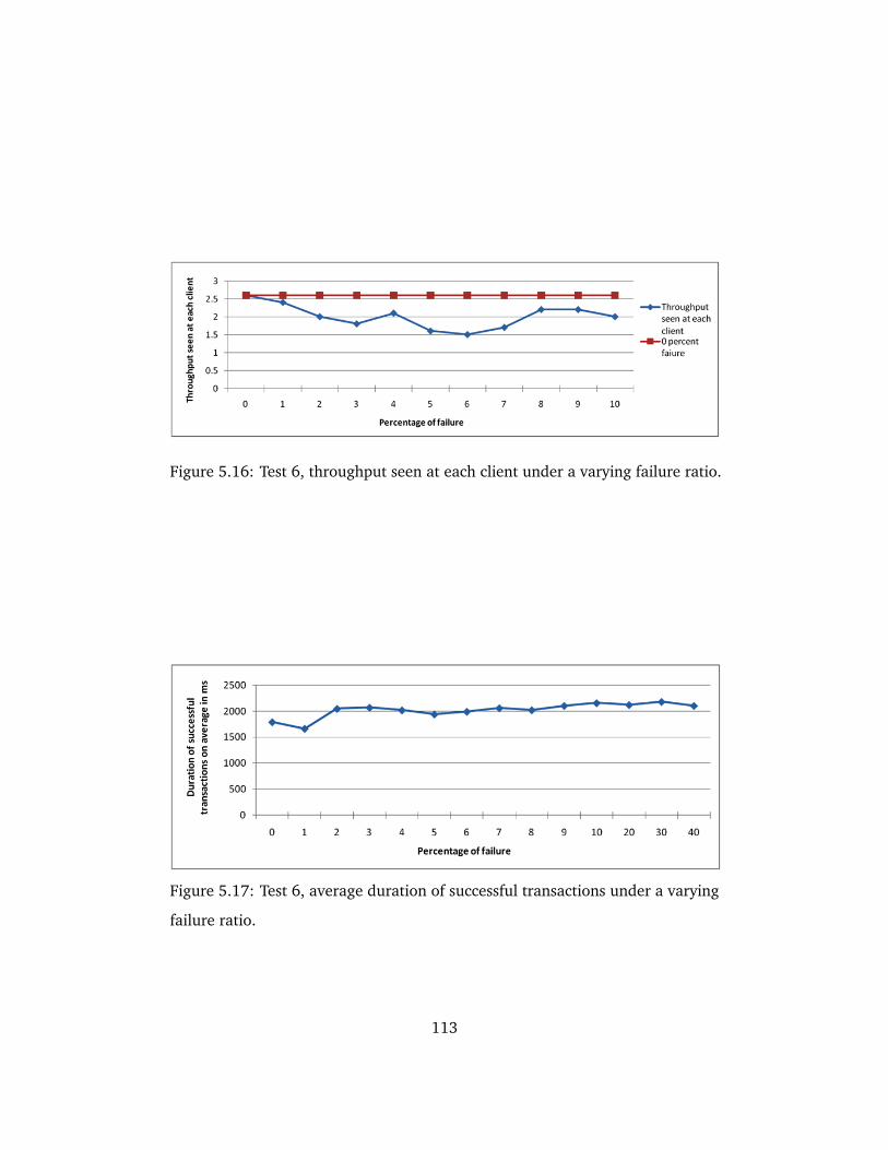
Figure 5.16: Test 6, throughput seen at each client under a varying failure ratio.

Figure 5.17: Test 6, average duration of successful transactions under a varying

failure ratio.

113

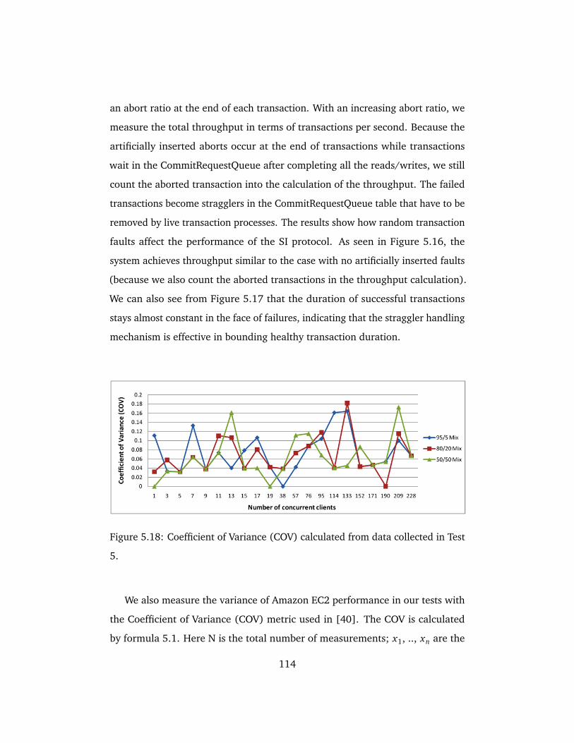
an abort ratio at the end of each transaction. With an increasing abort ratio, we

measure the total throughput in terms of transactions per second. Because the

artificially inserted aborts occur at the end of transactions while transactions

wait in the CommitRequestQueue after completing all the reads/writes, we still

count the aborted transaction into the calculation of the throughput. The failed

transactions become stragglers in the CommitRequestQueue table that have to be

removed by live transaction processes. The results show how random transaction

faults affect the performance of the SI protocol. As seen in Figure 5.16, the

system achieves throughput similar to the case with no artificially inserted faults

(because we also count the aborted transactions in the throughput calculation).

We can also see from Figure 5.17 that the duration of successful transactions

stays almost constant in the face of failures, indicating that the straggler handling

mechanism is effective in bounding healthy transaction duration.

Figure 5.18: Coefficient of Variance (COV) calculated from data collected in Test

5.

We also measure the variance of Amazon EC2 performance in our tests with

the Coefficient of Variance (COV) metric used in [40]. The COV is calculated

by formula 5.1. Here N is the total number of measurements; x1, .., xn are the

114

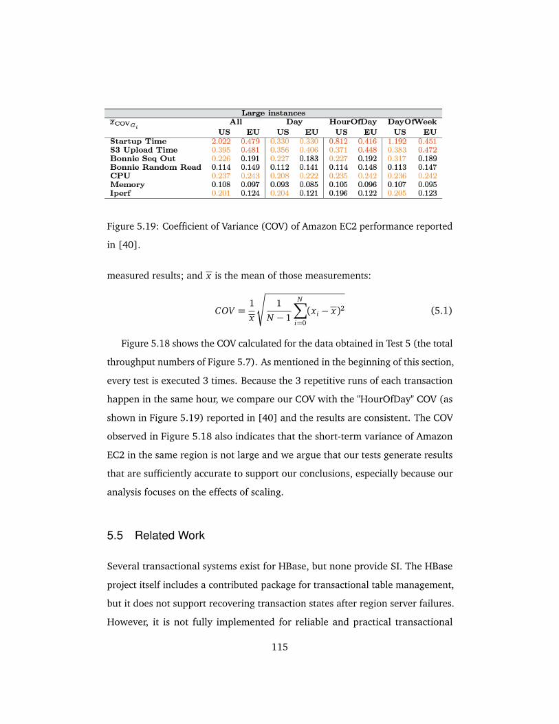
Figure 5.19: Coefficient of Variance (COV) of Amazon EC2 performance reported

in [40].

measured results; and x is the mean of those measurements:

COV =1

x

s

1

N − 1

N∑

i=0

(x i − x)2 (5.1)

Figure 5.18 shows the COV calculated for the data obtained in Test 5 (the total

throughput numbers of Figure 5.7). As mentioned in the beginning of this section,

every test is executed 3 times. Because the 3 repetitive runs of each transaction

happen in the same hour, we compare our COV with the "HourOfDay" COV (as

shown in Figure 5.19) reported in [40] and the results are consistent. The COV

observed in Figure 5.18 also indicates that the short-term variance of Amazon

EC2 in the same region is not large and we argue that our tests generate results

that are sufficiently accurate to support our conclusions, especially because our

analysis focuses on the effects of scaling.

5.5 Related Work

Several transactional systems exist for HBase, but none provide SI. The HBase

project itself includes a contributed package for transactional table management,

but it does not support recovering transaction states after region server failures.

However, it is not fully implemented for reliable and practical transactional

115

processing due to the lack of support for recovering transaction states after

region server failures and the possibility of lost updates for transactions with blind

writes. G-store [5] supports groups of correlated transactions over a pre-defined

set of data rows (called "Key Group") specified for each group of transactions

respectively. G-store does not support general transactions across all the data

tables and is suitable for applications that require transactional access to Key

Groups that are transient in nature with an assumption that the number of keys

in a Key Group must be small enough to be owned by a single node. CloudTPS

[42] implements a server-side middleware layer composed of programs called

local transaction managers (LTMs), but introduces extra overhead of middleware

deployment, data synchronization, and fault handling. Each LTM is responsible

for on-demand caching a subset of all data items. A transaction must specify the

row keys of all the data to be accessed at transaction start time and then sends

transaction request to any LTM to start a 2-phase commit protocol among all

the LTMs serving parts of the data items accessed by the transaction. CloudTPS

basically recreates another layer of small HBase-like region servers with data

loaded on-demand on top of HBase, introducing extra overhead of middleware

deployment, data synchronization, and fault handling. None of these systems

provides SI.

Only recently two relevant papers were published independently at almost

the same time about achieving snapshot isolation for distributed transactions, for

HBase and for BigTable: we published a paper describing our initial system (the

predecessor of the system described in this chapter) to support transactions with

SI on top of HBase [48], and Google published a paper about their system called

"Percolator" [36] supporting transactions with SI on top of BigTable. The two

systems share many design ideas yet are different in some major design choices.

HBaseSI is an extended and improved version of our initial system of [48].

It is similar to the initial system and similar to Google’s Percolator [36] in

116

that: all three systems are implemented as a client library rather than a set

of middleware programs and allow client transactions to decide autonomously

when they can commit (there is no central process to decide on commits); they

all rely on the multi-version data support from the underlying column store

for achieving snapshot isolation, and store transactional management data in

column store tables; they all make use of some centralized timestamp issuing

mechanism for generating globally well-ordered timestamps; and after starting

using either of the systems, users must use the systems for all the subsequent

data processing operations in order to guarantee data consistency. HBaseSI is

superior to the initial system of [48] in that: HBaseSI is the first system on HBase

to support global strong SI rather than the "gap-less" weak SI in the initial system;

it uses a completely different mechanism in handling distributed synchronization

(HBaseSI uses distributed queues to guarantee a correct sequence of transaction

execution, while the initial system uses a complicated and rather inefficient

mechanism to obtain snapshots); the initial system is inefficient because its

PreCommit table grows without bound and has to be searched in its entirety by

transactions attempting to commit; HBaseSI provides a simple mechanism for

handling stragglers, whereas handling stragglers for the system proposed in [48]

would be overly complicated.

In addition to the similarities listed above, HBaseSI shares with Percolator

its support of global strong SI. HBaseSI and Percolator are also very different

in several other aspects: HBaseSI focuses on random access performance with

low latency whereas Percolator focuses on analytical workloads that tolerate

larger latency; HBaseSI is non-intrusive to existing user data tables and stores the

version information and transaction information in extra system tables, whereas

Percolator is intrusive to existing user data and stores the same information

in two extra columns in every user tables (but this design decision of HBaseSI

makes it less scalable than Percolator concerning the number of concurrent

117

transactions), because Percolator distributes the transactional metadata to the

individual user data tables, rather than using a common set of global system

tables as in HBaseSI); HBaseSI supports non-blocking starts of transactions

and does not block reads, whereas Percolator may block reads while data is

being committed which may harm performance; HBaseSI strictly follows the

"first-committer-wins" rule, whereas Percolator does not and two concurrent

transactions with conflicting writesets could both fail; HBaseSI uses distributed

queues in handling synchronization and concurrency rather than using traditional

techniques such as data locks as in Percolator; and two concurrently committing

transactions could unnecessarily both fail in Percolator but not in HBaseSI. In

short, the two systems are designed with different purposes in mind and each

may excel at one aspect and not another. Note also that the protocol described

in Percolator cannot be trivially ported onto HBase, because HBase does not

support BigTable’s atomic single-row transactions, allowing multiple read-modify-

write operations to be grouped into one atomic transaction as long as they are

operating on the same row. HBase does not support the same functionality, but

rather, only supports single atomic row read or row write operations one at a

time, based on the row lock functionality (locking down a row exclusively against

concurrent reads/writes from all other parties).

5.6 Conclusions and Future Work

This chapter presents HBaseSI, a light-weight client library for HBase, enabling

multi-row distributed transactions with global strong SI on HBase user data

tables. There exists no other systems providing the same level of transactional

isolation on HBase yet. HBaseSI tries to achieve several design goals: achieving

global strong SI across table boundaries; being non-intrusive to existing user

data tables; strictly enforcing the "first-committer-wins" rule for SI; supporting

highly responsive transactions with no blocking reads; and employing an effective

118

straggler handling mechanism. The performance overhead of HBaseSI over HBase

is modest, especially for longer non-conflicting transactions involving a larger

number of read and write operations per transaction. Future research directions

may include implementing some helpful tools to optimize disk usage and possibly

extending HBaseSI to increase its scalability by distributing the transactional

metadata tables.

Concerning future work, HBaseSI can be further extended to support more

general range queries efficiently. We also plan to apply its design to other column

stores sharing similar architecture as HBase.

119

Chapter 6

Conclusions and Future Research

The theme of this thesis is enhancing data processing with Hadoop/HBase on

clouds. The PhD research started when cloud computing research was still in its

infancy and grid computing prevailed. Several preliminary research projects were

conducted around a light-weight grid computing system called "GridBASE", as

well as an early cloud computing case study for investigating the applicability of

using Hadoop to solve customized scientific data processing problems on clouds.

After these initial projects, Hadoop was chosen as the candidate framework for

further developing cloud data processing techniques. In the meantime, research

efforts were initiated by other researchers in the direction of enhancing Hadoop

for various data processing scenarios. This PhD thesis presents two main research

contributions in this research area.

The first contribution is CloudWF, a computational workflow system specifi-

cally targeted at cloud environments where Hadoop is installed. CloudWF is the

first workflow management system targeted to take advantage of the Hadoop/H-

Base architecture for scalability, fault tolerance and ease of use. It uses Hadoop

components to perform job execution, file staging and workflow information

storage. The novelty of the system lies in its ability to take full advantage of

121

what the underlying cloud computing framework can provide, and in its new

workflow description method that separates out workflow component dependen-

cies as standalone executable components for decentralized job execution and

transparent file staging over the MapReduce environment.

The second contribution is HBaseSI, a lightweight client library for HBase,

enabling multi-row distributed transactions with global strong SI on HBase user

data tables. HBaseSI is the first SI solution for HBase, and is implemented on top

of bare-bones HBase rather than deploying an extra middleware layer. HBaseSI

tries to achieve several design goals: achieving global strong SI across table

boundaries; being non-intrusive to existing user data tables; strictly enforcing the

"first-committer-wins" rule for SI; supporting highly responsive transactions with

no blocking reads; and employing an effective straggler handling mechanism.

The performance overhead of HBaseSI over HBase is modest, especially for

longer transactions involving a larger number of read and write operations per

transaction.

Apart from the two major contributions in the direction of enhancing Hadoop/H-

Base, we have also worked on a solution called "CloudBATCH" as supportive

work to tackle the problem of Hadoop’s incompatibility with existing cluster

batch job queuing systems. CloudBATCH uses Hadoop/HBase to assume the core

functionality of a cluster batch job queuing system, removing the complexity and

overhead of making the two kinds of systems compatible. We did not go into

details about CloudBATCH in this thesis because it deals with a rather practical

problem. But the issue CloudBATCH addresses is of practical importance and has

recently gained interest from researchers who are actively seeking for customized

solutions to be applied on TeraGrid, one of the major grid computing platforms

in the world.

Through these research contributions, we obtained fruitful results in designing

novel tools and techniques to extend and enhance the large-scale data processing

122

capability of Hadoop/HBase. As cloud computing becomes more and more

popular in academia and industry, we believe that there are promising future

research opportunities in further extending the data processing capability of

Hadoop/HBase on clouds for a wide spectrum of usage scenarios. In the following

sections, we will briefly describe some general future research directions.

6.1 Wireless Sensor Networks and Clouds

Wireless sensor networks (WSNs) are gaining increasing attention in various ap-

plication scenarios, such as environment monitoring, animal habitat surveillance,

the Internet of Things, etc. The potentially large amount of data gathered by

sensors and transmitted back to PC-hosts calls for novel and efficient data stor-

age and processing methods. Furthermore, a user-friendly programming model

and a corresponding task execution environment are still lacking, impeding fast

deployment and reprogramming of applications.

As a result, we consider wireless sensor network as a compelling application

area that will become a source of large amounts of data in the coming era of

ubiquitous mobile networks and the Internet of Things. It will be very interesting

to investigate the applicability of designing an integrated sensor network data

processing and programming platform backed by clouds, involving efficient

methods in storing and querying sensor data using HBase sparse tables, novel

methods based on HBase queries for extracting topology and routing information

and novel applications using the integrated environment, etc.

More specifically, for example, it may be interesting to design and implement

a cloud data processing system for sensor-gathered data. The system will make

use of existing hardware infrastructure (clusters/grids/clouds) for host data

processing. Due to the sparse nature of the sensor data, HBase sparse tables will

be used to manage data storage and querying. Hadoop MapReduce or existing

cluster batch job queuing system will be used to execute computing jobs. A

123

prototype task execution environment deployable to sensors (with TinyOS) can

also be developed, allowing users to program sensor actions.

6.2 Mobile Cloud

It is a trend that computing is becoming more and more mobile. How to efficiently

organize and make use of various types of mobile and smart devices may become

a next major research direction in cloud computing. Both hardware and software

platforms are needed to properly form a mobile cloud. Large industrial players

are moving into the mobile cloud area by leading industrial initiatives, such as

Google’s Cloud Printing, Microsoft’s SkyDrive and its "Project Hawaii" initiative

encouraging students at a selected number of universities to explore how to

"use the cloud to enhance the user experience on mobile devices." The new

HTML5 language is also believed to provide a convenient programming method

for developing and maintaining cloud-based mobile applications. Apart from

various enthusiastic efforts, many challenges still lie ahead. For example: how to

minimize data transfer over the air while pushing as much application logics as

possible into the cloud, how to agree on a unified set of programming primitives

across heterogenous mobile infrastructures for easy application development and

deployment, how to efficiently process data exploiting data locality and idling

mobile computing resources, etc. It is promising that some of the techniques

developed in grid/cloud computing can be exploited in the new mobile computing

context, which may further inspire novel methods rooted in the native mobile

computing infrastructure itself.

124

Bibliography

The numbers at the end of each entry list pages where the reference was cited.

In the electronic version, they are clickable links to the pages.

[1] Divyakant Agrawal, Amr El Abbadi, Shyam Antony, and Sudipto Das. Data

management challenges in cloud computing infrastructures. In DNIS, pages

1–10, Aizu, Japan, 03/2010 2010. Springer, Springer. 66

[2] Philip A. Bernstein, Vassos Hadzilacos, and Nathan Goodman. Concurrency

Control and Recovery in Database Systems. Addison Wesley Publishing

Company, 1987. 66

[3] Cascading. http://www.cascading.org/. Retrieved April 15, 2011. 56

[4] Fay Chang, Jeffrey Dean, Sanjay Ghemawat, Wilson C. Hsieh, Deborah A.

Wallach, Mike Burrows, Tushar Chandra, Andrew Fikes, and Robert E.

Gruber. Bigtable: A distributed storage system for structured data. In OSDI,

pages 205–218, 2006. 2, 12

[5] Sudipto Das, Divyakant Agrawal, and Amr El Abbadi. G-store: a scalable

data store for transactional multi key access in the cloud. In Proceedings

of the 1st ACM symposium on Cloud computing, SoCC ’10, pages 163–174,

New York, NY, USA, 2010. ACM. 66, 116

125

[6] Hive: A data warehouse infrastructure that provides data summarization

and ad-hoc querying. The Apache Software Foundation. http://hive.

apache.org/. Retrieved April 15, 2011. 2

[7] C. J. Date. An Introduction to Database Systems, Fifth Edition. Addison

Wesley Publishing Company, 2003. 66

[8] Khuzaima Daudjee and Kenneth Salem. Lazy database replication with

snapshot isolation. In Proceedings of the 32nd international conference on

Very large data bases, VLDB ’06, pages 715–726. VLDB Endowment, 2006.

69

[9] H. De Sterck, R.S. Markel, T. Pohl, and U. Ruede. A lightweight Java

Taskspaces framework for scientific computing on computational grids. In

Proceedings of the ACM Symposium on Applied Computing, Track on Parallel

and Distributed Systems and Networking, 2003. 22

[10] Hans De Sterck, Alex Papo, Chen Zhang, Micah Hamady, and Rob Knight.

Database-driven grid computing and distributed web applications: A com-

parison. In Grids for Bioinformatics and Computational Biology. Wiley, 2007.

19, 24

[11] Hans De Sterck, Chen Zhang, and Aleks Papo. Database-driven grid com-

puting with GridBASE. In The 2007 IEEE International Symposium on

Bioinformatics and Life Science Computing (BLSC2007), 2007. 19, 22, 24

[12] Jeffrey Dean and Sanjay Ghemawat. MapReduce: Simplified data process-

ing on large clusters. In OSDI, pages 137–150, 2004. 2, 12

[13] Ewa Deelman, Gurmeet Singh, Mei-Hui Su, James Blythe, Yolanda Gil,

Carl Kesselman, Gaurang Mehta, Karan Vahi, G. Bruce Berriman, John

Good, Anastasia Laity, Joseph C. Jacob, and Daniel S. Katz. Pegasus:

126

a framework for mapping complex scientific workflows onto distributed

systems. Scientific Programming Journal, 13:219–237, 2005. 39

[14] Xavier Défago, André Schiper, and Péter Urbán. Total order broadcast

and multicast algorithms: Taxonomy and survey. ACM Computing Surveys,

36:2004, 2003. 66

[15] Amazon Elastic Compute Cloud (Amazon EC2). http://aws.amazon.

com/ec2/. Retrieved April 15, 2011. 2, 10, 39

[16] Fatima Farag, Moustafa Hammad, and Reda Alhajj. Adaptive query process-

ing in data stream management systems under limited memory resources.

In Proceedings of the 3rd workshop on Ph.D. students in information and

knowledge management, PIKM ’10, pages 9–16, New York, NY, USA, 2010.

ACM. 58, 66

[17] I. Foster, C. Kesselman, and S. Tuecke. The anatomy of the grid: Enabling

scalable virtual organizations. International Jounral of Supercomputer Ap-

plications, 15, 2001. 9, 39

[18] Sanjay Ghemawat, Howard Gobioff, and Shun-Tak Leung. The Google File

System. In SOSP, pages 29–43, 2003. 2, 12

[19] Jim Gray and U. C. Berkeley. A critique of ANSI SQL isolation levels. In

SIGMOD, pages 1–10. ACM Press, 1995. 69, 70

[20] Hadoop On Demand (HOD): A system for provisioning virtual Hadoop

clusters over a large physical cluster. The Apache Software Foundation.

http://hadoop.apache.org/common/docs/r0.17.0/hod.html. Re-

trieved April 15, 2011. 31

[21] HBase: An open-source distributed column-oriented store. The Apache

Software Foundation. http://hadoop.apache.org/. Retrieved April 15,

2011. 2, 14

127

[22] Pat Helland. Life beyond distributed transactions: an apostate’s opinion. In

Conference on Innovative Data Systems Research, pages 132–141, 2007. 66

[23] Pig: A high-level data-flow language and execution framework for paral-

lel computation. The Apache Software Foundation. http://pig.apache.

org/. Retrieved April 15, 2011. 2, 56

[24] C. Hoffa, G. Mehta, T. Freeman, E. Deelman, K. Keahey, B. Berriman,

and J. Good. On the use of cloud computing for scientific workflows. In

Proceedings of the 2008 Fourth IEEE International Conference on eScience,

pages 640–645, 2008. 39

[25] Ryan Kennedy, Manuel E. Lladser, Zhiyuan Wu, Chen Zhang, Michael Yarus,

Hans De Sterck, and Rob Knight. Natural and artificial RNAs occupy the

same restricted region of sequence space. RNA, 16:280–289, 2010. 19, 24

[26] Leslie Lamport. Generalized consensus and paxos. In Microsoft Research

Technical Report MSR-TR-2005-33, 2005. 66

[27] B. Ludscher, I. Altintas, C. Berkley, D. Higgins, E. Jaeger, M. Jones, E. Lee,

J. Tao, and Y. Zhao. Scientific workflow management and the Kepler

system. Concurrency and Computation: Practice and Experience, 18:1039–

1065, 2006. 39, 40, 58

[28] Mahout: A Scalable machine learning and data mining library. The Apache

Software Foundation. http://mahout.apache.org/. Retrieved April 15,

2011. 3

[29] S. Majithia, M. Shields, I. Taylor, and I. Wang. Triana: A graphical web

service composition and execution toolkit. In Proc. IEEE Intl. Conf. Web

Services (ICWS), pages 514–524, 2004. 39, 40

[30] T. Oinn, M. Greenwood, M.J. Addis, M.N. Alpdemir, J. Ferris, K. Glover,

C. Goble, A. Goderis, D. Hull, D.J. Marvin, P. Lord P. Li, M.R. Pocock,

128

M. Senger, R. Stevens, A. Wipat, and C. Wroe. Taverna: Lessons in creating

a workflow environment for the life sciences. Concurrency and Computation:

Practice and Experience, 18:1067–1100, 2002. 39, 40

[31] C. Olston, B. Reed, U. Srivastava, R. Kumar, and A. Tomkins. Pig Latin: a

not-so-foreign language for data processing. In Proceedings of the 2008 ACM

SIGMOD international conference on Management of data, pages 1099–1110,

2008. 56

[32] TeraByte Sort on Apache Hadoop. http://www.hpl.hp.com/hosted/

sortbenchmark/YahooHadoop.pdf. Retrieved April 15, 2011. 2, 14

[33] Yahoo! Oozie. http://issues.apache.org/jira/browse/

HADOOP-5303. Retrieved April 15, 2011. 56

[34] Hadoop: An open-source implementation of Google’s MapReduce program-

ming paradigm and job execution framework. The Apache Software Foun-

dation. http://hadoop.apache.org/. Retrieved April 15, 2011. 2, 13

[35] Oracle. Sun grid engine with Hadoop integration. http://wikis.sun.

com/display/gridengine62u5/Using+the+Hadoop+Integration.

Retrieved April 15, 2011. 31

[36] Daniel Peng and Frank Dabek. Large-scale incremental processing using

distributed transactions and notifications. In Proceedings of the 9th USENIX

conference on Operating systems design and implementation, OSDI’10, pages

1–15, Berkeley, CA, USA, 2010. USENIX Association. 22, 66, 100, 116

[37] The Condor project. Support high throughput computing (HTC) on large

collections of distributively owned computing resources. http://www.cs.

wisc.edu/condor/. Retrieved April 15, 2011. 58

129

[38] The Pegasus project. A set of technologies that help workflow-based ap-

plications execute in a number of different environments including desk-

tops, campus clusters, grids, and clouds. http://pegasus.isi.edu/. Re-

trieved April 15, 2011. xviii, 58, 59, 60

[39] R. Ranjan, M. Rehman, and R. Buyya. A decentralized and cooperative

workflow scheduling algorithm. In Proc. 8th Intl. Conf. on Cluster Computing

and the Grid (CCGrid), 2008. 4, 43

[40] Jörg Schad, Jens Dittrich, and Jorge-Arnulfo Quiané-Ruiz. Runtime mea-

surements in the cloud: observing, analyzing, and reducing variance. Proc.

VLDB Endow., 3:460–471, September 2010. xix, 98, 114, 115

[41] Hadoop Streaming. http://hadoop.apache.org/common/docs/r0.15.

2/streaming.html. Retrieved April 15, 2011. 57

[42] Zhou Wei, Guillaume Pierre, and Chi-Hung Chi. Scalable transactions for

web applications in the cloud. In Proceedings of the 15th International

Euro-Par Conference on Parallel Processing, Euro-Par ’09, pages 442–453,

Berlin, Heidelberg, 2009. Springer-Verlag. 116

[43] J. Yu and R. Buyya. A taxonomy of scientific workflow systems for grid

computing. SIGMOD Record, 34:44–49, 2005. 39

[44] Matei Zaharia, Dhruba Borthakur, Joydeep Sen Sarma, Khaled Elmeleegy,

Scott Shenker, and Ion Stoica. Delay scheduling: A simple technique for

achieving locality and fairness in cluster scheduling. In Proceedings of the

5th European conference on Computer systems, EuroSys ’10, pages 265–278,

2010. 34

[45] Chen Zhang, Ashraf Aboulnaga, Hans De Sterck, Haig Djambazian, and Rob

Sladek. Case study of scientific data processing on a cloud using Hadoop.

In High Performance Computing Symposium (HPCS2009), 2009. 20, 25, 30

130

[46] Chen Zhang and Hans De Sterck. CloudWF: A computational workflow

system for clouds based on Hadoop. In The First International Conference

on Cloud Computing (CloudCom2009), 2009. 4, 20

[47] Chen Zhang and Hans De Sterck. CloudBATCH: A batch job queuing

system on clouds with Hadoop and HBase. In The Second IEEE International

Conference on Cloud Computing Technology And Science (CloudCom2010),

2010. 22, 30, 35, 36

[48] Chen Zhang and Hans De Sterck. Supporting multi-row distributed transac-

tions with global snapshot isolation using bare-bones HBase. In The 11th

ACM/IEEE International Conference on Grid Computing (Grid2010), 2010.

4, 22, 66, 116, 117

[49] Chen Zhang and Hans De Sterck. HBaseSI: A solution for multi-row dis-

tributed transactions with global strong snapshot isolation on clouds. Scal-

able Computing: Practice and Experience, 12, July 2011. 4, 22

131