Embed Size (px)
Citation preview

Published by World Academic Press, World Academic Union
ISSN 1746-7659, England, UK
Journal of Information and Computing Science
Vol. 11, No. 3, 2016, pp.214-234
Enhancement of Performance of TCP Using Normalised
Throughput Gradient in Wireless Networks
N.G.Goudru1 and B.P.Vijaya kumar2
1 Department of MCA, BMS Institute of Technology
(affiliated to Visvesvaraya Technological University), Bangalore, India. Mobile: 90-9341384414,E-mail: [email protected].
2 Department of Information Science and Engineering, MS Ramaiah Institute of Technology
(affiliated to Visvesvaraya Technological University), Bangalore, India.
Mobile:90-9980634134, E-mail: [email protected]
(Received May 01, 2016, accepted June 14, 2016)
Abstract. Transmission control protocol (TCP) is a dominant transport layer protocol for reliable data
delivery in the internet. When packet loss occurs, TCP makes an implicit assumption that all packet loss is
due to congestion. This results in unnecessary degradation in the TCP performance while traversing over a
wireless link. In this paper, to improve the performance of TCP, we use NTG loss-predictor to distinguish
congestion loss from transmission loss. Based on the prediction of type of loss, an appropriate algorithm is
invoked by using NTG loss-prediction parameter β. Frequency of congestion loss and wireless loss
predictions are analysed. Performance of TCP is improved further by discussing stability analysis over the
system. A time-delay control theory is used and by constructing Hermit matrix, analysis is made for
asymptotic stability of the system. Explicit conditions are derived for Pmax (RED controller) and β (NTG loss
controller) in terms of wireless network parameters. Using the characteristic equation of the matrix,
convergence of the queue length at the bottleneck router is discussed. Analysis of convergence of queue
length to a given target value is analysed. This establishes stability in the router performance. An
approximate solution of queue length is derived. Our results provide better solutions for global stability and
convergence conditions of the system.
Keywords: congestion-loss, convergence, immediate-recovery, loss-predictor, stability, transmission-loss,
wireless-networks.
1. Introduction
Realistically, the existing Internet service uses the combination of wired and wireless media for
communication, and is called as heterogeneous network. In wireless networks, packet losses are due to
congestion and high bit error rate transmission over the wireless link. TCP, a widely used transport protocol,
performs satisfactorily over wired networks and fails to perform well in the wireless networks because it is
not be able to differentiate the loss caused by congestion or transmission. When a packet loss occurs during
wireless transmission, TCP diagnoses it as a congestion event and reduce the flow rate. This policy will
affect the performance of TCP and results in considerable degrade over wireless link [1], [2], [3], [20]. To
improve the performance of TCP over wireless network, many techniques are proposed by the researchers.
Some of them are, (i) I-TCP (Indirect TCP) - use two different links in the base station. One link is from
base station to the mobile station and the other one is from wired host to the base station. Using wired link
the base station receives data from the source and transmits the data to the mobile station using wireless link
which feels like sending the data by using wired link [4]. (ii) M-TCP (Mobile TCP)-has the facility of
keeping a retransmission timer in the base station. This timer is used by the sender TCP for checking the
time-out period. For each receive of the data packet, base station sends an acknowledgement packet to the
source before the timer period expires [5]. (iii) SNOOP is data link layer assisted protocol used to improve
the performance of TCP in wireless networks (environment). The base station keeps track of all the packets
transmitted from a source TCP. Base station keeps a copy of the packet in its buffer till it receives the
acknowledgement. It removes the packet from its buffer after acknowledgement is received. When a packet
loss occurs because of wireless transmission error, base station retransmits the lost packet. SOONP protocol
does not answer for time-out event occurrence in mobile wireless transmission or the duplicate
acknowledgements [6]. (iv) ELN (Explicit Loss Notification)-keeps the wireless loss information in the base
Journal of Information and Computing Science, Vol. 11(2016) No. 3, pp 214-234
JIC email for subscription: [email protected]
215
station, and the base station sets the ELN bit to the duplicate acknowledgement. For the ELN-set duplicate
acknowledgement, source TCP assumes that the packet loss is due to wireless transmission error and does
not decrease its window size which results in congestion [7]. (v) W-TCP (Wireless-TCP)-is a rate-based
wireless congestion control protocol. W-TCP assumes that the packet losses due to burst traffic as router
congestion and random losses as the wireless transmission error. In each case, the receiver measures the time
interval of the received packets and communicates the source to control the sending rate by using this time
interval estimate. [8]. (vi) TCP Westwood- is a sender-side modification for wireless TCP. From the
acknowledgement packet received, the sender estimates the current sending rate. For the congestion
notification, the sender decides the congestion window size from the estimated sending rate. TCP Westwood
has problem in time estimation and needs a fine-grained timer. In a dynamically changing network, the
estimation cannot be accurate [9]. (vii) The ACK Pacing algorithm - can be used for black-out and hand-off
delays. By sending ACK Pacing packets, burst data delivery is prevented from old path and the route update
for new path [10]. (viii) JTCP (Jitter-based)-JTCP method is for heterogeneous wireless networks to adopt
sending rates to the packet losses and jitter ratios [11]. (ix) ACK-Splitting-improves the TCP throughput
over wired and wireless heterogeneous networks [12]. However, these schemes may not have good
performance or fairness or it is too complex to deploy in wireless systems. To satisfy these challenges and
for applying TCP over wireless link, we propose a model based scheme that can dynamically change the
sending rate to the packet loss due to congestion and transmission. The model has integrated with the
capability of distinguishing the packet losses due to congestion or transmission. If the loss is due to
congestion, congestion control algorithm is invoked to reduce the network congestion and when the loss is
due to transmission, immediate-recovery algorithm is invoked to recover from the decreased flow rate. One
of the popular congestion avoidance schemes called RED (random early detection) and an accurate loss-
predictor function called NTG loss-predictor which is designed based on CAT are used in the system model.
Congestion avoidance technique (CAT) monitors the level of congestion in the network, and instructs the
source that the sender window should be increased or decreased and vice versa. A TCP source understands
that a particular packet has lost due to congestion or due to wireless transmission error and take appropriate
action [18]. To enhance performance of TCP for further, we apply stability [13], [14], [22]. A time-delay
control theory is used and hermit matrix method is applied to analyse the asymptotic stability. A relationship
between RED parameter pmax and NTG loss-predictor parameter β is established. The stability boundaries
are established in terms of wireless network parameters. The work is further enhanced by analysing the
queue convergence at the ingress point of the bottleneck link. Using characteristic equation of the Hermite
matrix, an approximate solution for the instantaneous queue length, q(t) is derived. The convergence
boundaries of q0, pmax and β are presented. Using these boundary values, convergence analysis of the queue
length for a given target value is discussed. The helps in maintaining RED router stable. Using Matlab
numerical results are given to validate the analytical results. The above illustrated characteristics collectively
make TCP robust by minimising the packet losses and maximising throughput. Our results provide global
stability and convergence conditions of the system.
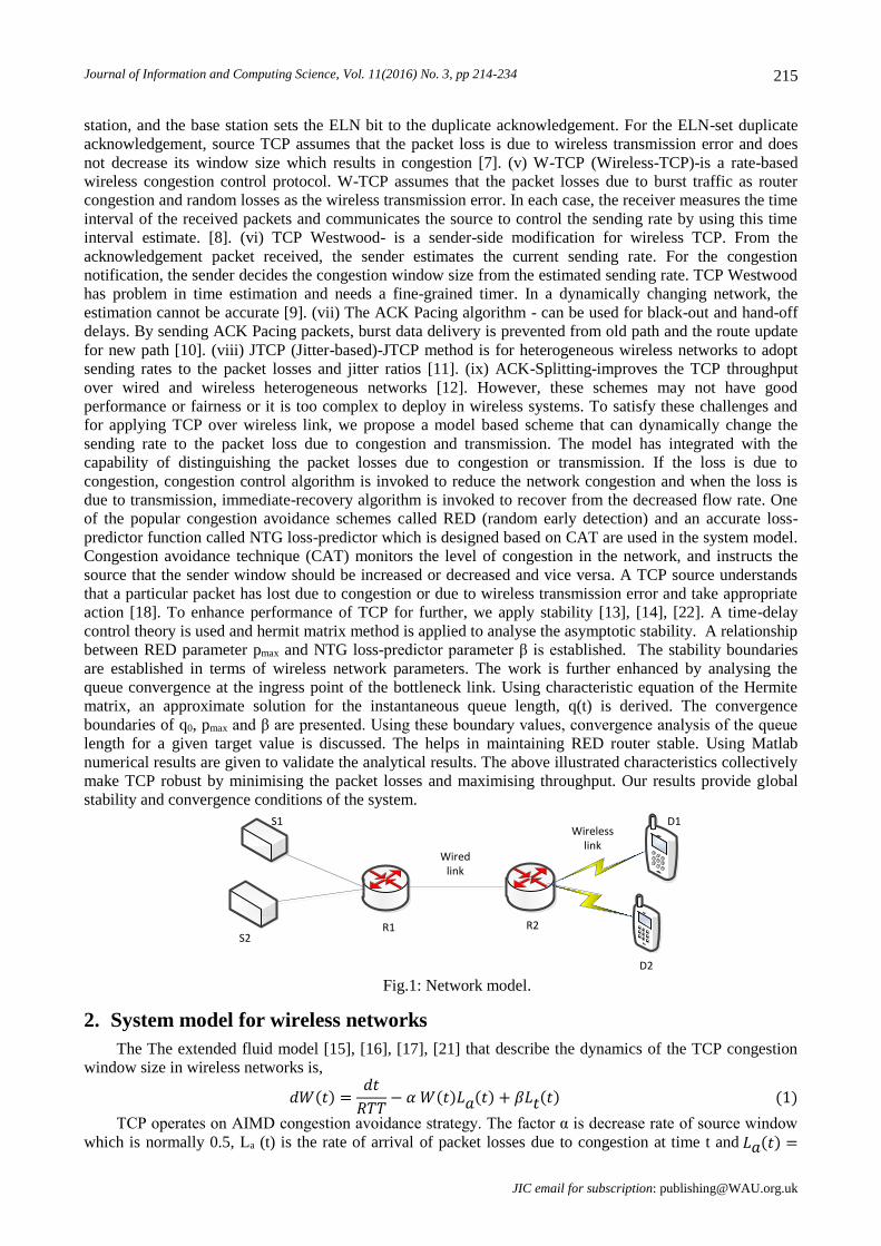
S1
S2R1 R2
D1
D2
Wireless link
Wired link
Fig.1: Network model.
2. System model for wireless networks
The The extended fluid model [15], [16], [17], [21] that describe the dynamics of the TCP congestion
window size in wireless networks is,
𝑑𝑊(𝑡) =𝑑𝑡
𝑅𝑇𝑇− 𝛼 𝑊(𝑡)𝐿𝑎(𝑡) + 𝛽𝐿𝑡(𝑡) (1)
TCP operates on AIMD congestion avoidance strategy. The factor α is decrease rate of source window
which is normally 0.5, La (t) is the rate of arrival of packet losses due to congestion at time t and 𝐿𝑎(𝑡) =

N.G.Goudru et al.: Enhancement of Performance of TCP Using Normalised Throughput Gradient in Wireless Networks
JIC email for contribution: [email protected]
216
𝑤(𝑡−𝑅(𝑡))
𝑅(𝑡−𝑅(𝑡)) 𝑝(𝑡 − 𝑅(𝑡 − 𝑅(𝑡))). This loss is proportional to the throughput at the source. First term on the right
hand side of equation (1) refers to exponential increase of the sender window size until congestion occurs at
the destination. The second term refers to congestion avoidance scheme based on RED. The third term Lt(t)
refers to immediate-recovery due to transmission loss. The transmission loss is proportional to the sending
rate of the source. Therefore, Lt (t) is proportional to 𝑤(𝑡−𝑅(𝑡))
𝑅(𝑡−𝑅(𝑡)).
The equation (1) can be modified to, 𝜕𝑤
𝜕𝑡=
1
𝑅(𝑡)−𝑤(𝑡)𝑤(𝑡−𝑅(𝑡))
2𝑅(𝑡−𝑅(𝑡))𝑝(𝑡 − 𝑅(𝑡)) + 𝛽
𝑤(𝑡−𝑅(𝑡))
𝑅(𝑡−𝑅(𝑡)) (2)
β is called NTG loss-predictor parameter. It has some constant rate of transmission-loss and by choice β
ϵ[0,1]. The differential version of Lindley’s equation for capturing the dynamic behaviour of instantaneous
queue length is given by, 𝜕𝑞(𝑡)
𝜕𝑡= 𝑁 𝑤(𝑡)
𝑅(𝑡)− 𝐶𝑑
(3)
Where, w(t)/R(t) is increase in queue length due to arrival of the packets from N- TCP flows. The
down-link capacity, Cd = q(t)/R(t) is the decreasing factor in queue length due to servicing of the packets and
delay of the packet departure from the router. The service time is variable. One of the most important
advantages of using instantaneous queue length over average queue length is faster detection of congestion.
The mathematical version of RED scheme for dropping packets with probability is given by,
𝑃(𝑡) =
{
0 , 𝑞(𝑡) ∈ [0, 𝑡𝑚𝑖𝑛]
𝑞(𝑡)−𝑡𝑚𝑖𝑛𝑊𝑚𝑎𝑥−𝑡𝑚𝑖𝑛
𝑃𝑚𝑎𝑥 , 𝑞(𝑡) ∈ [𝑡𝑚𝑖𝑛,𝑊𝑚𝑎𝑥]
1 , 𝑞(𝑡) ≥ 𝑊𝑚𝑎𝑥
(4)
Congestion loss is assumed to take place when queue buffer of the router reaches a value of Wmax
packets. The maximum buffer size, Wmax of the router is given by, 𝑊𝑚𝑎𝑥 = 𝐶𝑑𝑆 𝑅(𝑡) +𝑀 , Where Cd /S is
the bandwidth delay product, M (in packets) is the buffer size of the router, R(t) is the round trip time. The
buffer overflow takes place when the congestion window size becomes larger than Wmax value. Cd is the
down-link bandwidth. The model describing round trip time (RTT) in wireless networks is given by, (𝑡) =
𝑞(𝑡)
𝐶𝑑+ 𝑇𝑝 , Tp is the propagation delay in the wireless media, q(t)/Cd models the queuing delay.
2.1. Normalised throughput gradient (NTG)
NTG is a metric used to deduce the traffic load from the acknowledgements. When a TCP connection
has no data to transmit, then other TCP sources detect the change using NTG metric and absorb the released
resources. When a source initiates a connection, the window is set to one packet, after receiving an
acknowledgement, the scheme checks the NTG. (i) If the NTG is lesser than the NTG threshold value,
sender window enters the increased mode. (ii) If the NTG is greater than or equal to the NTG threshold value,
increase the cwnd (sender window size) by one packet [18]. Wang and Crowcroft [19] proposed a congestion
avoidance method based on normalised throughput gradient (fNTG). Let Pi be the ith monitored packet. The
throughput gradient of Pi is given by 𝑇𝐺𝑖 =𝑇𝑖−𝑇𝑖−1𝑊𝑖−𝑊𝑖−1
The normalised throughput gradient,
𝑓𝑁𝑇𝐺 =𝑇𝐺𝑖𝑇𝐺1
But, 𝑇𝐺1 =𝑇1−𝑇0𝑊1−𝑊0
=1
𝑅𝑇𝑇𝑖
Chose,
𝑤0 = 0,𝑤1 = 1, 𝑇0 = 0, 𝑎𝑛𝑑 𝑇1 =𝑤1𝑅𝑇𝑇1
=1
𝑅𝑇𝑇1
Thus, 𝑓𝑁𝑇𝐺 =𝑇𝐺𝑖1
𝑅𝑇𝑇𝑖
After substitution and simplification, we get

Journal of Information and Computing Science, Vol. 11(2016) No. 3, pp 214-234
JIC email for subscription: [email protected]
217
𝑓𝑁𝑇𝐺 =𝑅𝑇𝑇𝑖
(𝑊𝑖 −𝑊𝑖 − 1)(𝑊𝑖𝑅𝑇𝑇𝑖
−𝑊𝑖 − 1𝑅𝑇𝑇𝑖 − 1
)
The NTG loss-predictor is a congestion avoidance technique. It uses throughput values to determine
the cause of a packet loss. As the traffic load changes NTG value varies over the range [1, 0]. Under light
traffic, the NTG value is around 1. NTG value decreases gradually for the increase in traffic load, and
reaches 0 when the path is saturated. When the resources captured by a TCP session are released, the NTG
value increases substantially. Without loss of generality we choose NTG threshold value as 0.5. i) If fNTG < ½, the loss of next packet is due to congestion.
ii) if fNTG ≥1/2, the loss of next packet is due to transmission.
When the source detect that loss is due congestion, NTG parameter, β=0. The threshold value of sender
window is fixed to half of the current window size and slow start phase started. When source detects that loss
is due to wireless transmission, a loss recovery module called Immediate-recovery algorithm gets invoked,
where sender window size is added with β-times the sending rate in the previous RTT.
3. Time-delay feedback control system
In this section, we study the asymptotic stability of TCP in wireless network system. The aim is to save
the network system from congestion and decrease the packet losses accruing due to congestion. The
implement methodology involves (i) linearizing the system models, (ii) using the Hermite matrix for time-
delay control system, explicit conditions under which the system is asymptotically stability are obtained. A
relationship between RED parameter Pmax and NTG parameter β is derived. The stability regions for Pmax
and β in terms of wireless TCP parameters are obtained.
3.1. Linear model derivation
Let x(t) be a general non-linear function defined by,𝑥(𝑡) = 𝑓(𝑢(𝑡), 𝑣(𝑡), 𝑡), where, u(t) represents the
sender window dynamics, and v(t) represent the queue dynamics at the bottleneck link. Assuming
that 𝑓(𝑢(𝑡), 𝑣(𝑡), 𝑡) has smooth and continuous derivatives around the equilibrium point, 𝑄0 =(𝑤0, 𝑅0, 𝑞0, 𝑝0). Using Taylor’s series expansion, the linear function of non-linear function, ignoring second
and higher order partial derivatives is,
𝑓(𝑢(𝑡), 𝑣(𝑡), 𝑡) = 𝑓(𝑢0(𝑡), 𝑣0(𝑡), 𝑡0) + 𝑓𝑢(𝑡)𝛿𝑢(𝑡) + 𝑓𝑣(𝑡)𝛿𝑣(𝑡) + 𝑂(𝛿𝑢(𝑡), 𝛿𝑣(𝑡))
where (𝑡) =𝜕𝑓
𝜕𝑢|(𝑢0, 𝑣0) , 𝑓𝑣(𝑡) =
𝜕𝑓
𝜕𝑣|(𝑢0, 𝑣0) .
The linear models of the equations (2) to (4) are derived around the equilibrium point 𝑄0 =(𝑤0, 𝑅0, 𝑞0, 𝑝0). Let N be the number of TCP flows and R be the round trip time which are considered as
constants. At the equilibrium point Q0, the steady state conditions of equations (2) and (3) are given by
�̇�(𝑡) = 0, �̇�(𝑡) = 0.
The estimation algorithm is based on small signal behaviour dynamics, therefore, at the equilibrium
point, without loss of generality, we can assume,
𝑤(𝑡) = 𝑤(𝑡 − 𝑅(𝑡)) = 𝑤0, 𝑞(𝑡) = 𝑞(𝑡 − 𝑅(𝑡)) = 𝑞0, 𝑝(𝑡) = 𝑝(𝑡 − 𝑅(𝑡)) = 𝑝0,
𝑅(𝑡) = 𝑅(𝑡 − 𝑅(𝑡)) = 𝑅0 (5)
Using equations (5) in �̇�(𝑡) = 0, �̇�(𝑡) = 0, and after simplification we get,
𝑝0 =2𝛽𝑤0 + 2
𝑤02 , 𝑤0 =
𝑅0𝐶𝑑𝑁
, 𝑁 =𝑅0𝐶𝑑𝑤0
Let, 𝑤𝑅 = 𝑤(𝑡 − 𝑅(𝑡)), 𝑝𝑅 = 𝑝(𝑡 − 𝑅(𝑡)). From (2) we get,
𝑢(𝑤,𝑤𝑅, 𝑞, 𝑝𝑅) = 1
𝑅(𝑡)−𝑤(𝑡)𝑤𝑅(𝑡)
2𝑅(𝑡)𝑝(𝑡 − 𝑅(𝑡)) + 𝛽
𝑤𝑅(𝑡)
𝑅(𝑡) (6)
To linearize equation (6), find all the partial derivatives of u(w,wR,q,pR) with respect to the variables at
the equilibrium point and defining,
𝛿𝑤(𝑡) = 𝑤(𝑡) − 𝑤0, 𝛿𝑞(𝑡) = 𝑞(𝑡) − 𝑞0, 𝛿𝑝(𝑡) = 𝑝(𝑡) − 𝑝0 𝛿�̇�(𝑡) = �̇�(𝑡) − 𝑤0, 𝛿�̇�(𝑡) = �̇�(𝑡) − 𝑞0
𝛿𝑝(𝑡) =𝐿
𝐵(𝑞(𝑡) − 𝑡𝑚𝑖𝑛) − 𝑝0 , where B= Wmax – tmin , L=pmax
𝛿�̇�(𝑡) = −(𝛽
𝑅0+
2𝑁
𝑅02 𝐶𝑑
) 𝛿𝑤 − 𝐶𝑑2 𝑅02𝑁2
𝛿𝑝𝑅 (7)

N.G.Goudru et al.: Enhancement of Performance of TCP Using Normalised Throughput Gradient in Wireless Networks
JIC email for contribution: [email protected]
218
𝛿�̇�(𝑡) =𝑁
𝑅0𝛿𝑤(𝑡) −
1
𝑅0𝛿𝑞(𝑡) (8)
𝛿𝑝(𝑡 − 𝑅0) = 𝐿
𝐵(𝛿𝑞(𝑡 − 𝑅0)) +
𝐿
𝐵(𝑞0 − 𝑡𝑚𝑖𝑛) − 𝑝0 (9)
Using equation (9) in (7), we get
𝛿�̇�(𝑡) = −(𝑅0𝑤0
+2𝑁
𝑅02 𝐶𝑑) 𝛿𝑤(𝑡) −
𝐿𝐶𝑑2𝑅02𝑁2𝐵
𝛿𝑞(𝑡 − 𝑅0) +𝐿𝐶𝑑2𝑅02𝑁2𝐵
(𝑡𝑚𝑖𝑛 − 𝑞0)
+ 𝑅0𝐶𝑑2𝑝0 2𝑁2
(10)
Denote, 𝑥(𝑡) = [𝛿𝑤(𝑡)𝛿𝑞(𝑡)
] , then �̇�(𝑡) = 𝐴𝑥(𝑡) + 𝐸𝑥(𝑡 − 𝑅(𝑡)) + 𝐹 (11)
Where,
𝐴 = [−(
𝛽
𝑅0+
2𝑁
𝑅02 𝐶𝑑
) 0
𝑁
𝑅0
−1
𝑅0
] 𝐸 = [0
−𝐿𝑅0𝐶𝑑2
2𝑁2𝐵
0 0] , 𝐹 = [
−𝐿𝑅0𝐶𝑑2
2𝑁2𝐵(𝑡𝑚𝑖𝑛 − 𝑞0) +
𝑅0 𝐶𝑑2𝑝0
2𝑁2
0]
Solving linear differential equation (11) using Laplace transform technique with L{x(t)} = x(s), we get
(𝑠𝐼 − 𝐴 − 𝐸𝑒−𝑅0𝑠)𝑥(𝑠) =𝐹
𝑠 (12)
The characteristic equation of (12) is, |𝑠𝐼 − 𝐴 − 𝐸𝑒−𝑅0𝑠| = 0 (13)
After simplification,
𝑠2 + (𝛽
𝑅0+
2𝑁
𝑅02𝐶𝑑
+1
𝑅0) 𝑠 + (
𝛽
𝑅02+
2𝑁
𝑅03 𝐶𝑑
+𝐿𝐶𝑑
2
2𝑁𝐵𝑒−𝑅0𝑠) = 0 (14)
The characteristic equation (14) determines the stability of the closed-loop time-delay wireless system
in terms of the state variables𝛿𝑤(𝑡) 𝑎𝑛𝑑 𝛿𝑞(𝑡).
3.2. Stability analysis
Denote, 𝑃(𝑠, 𝑒−𝑅0𝑠) = 𝑠2 + (𝛽
𝑅0+
2𝑁
𝑅02𝐶𝑑
+1
𝑅0) 𝑠 + (
𝛽
𝑅02+
2𝑁
𝑅03 𝐶𝑑
+𝐿𝐶𝑑
2
2𝑁𝐵𝑒−𝑅0𝑠)
Let 𝑒−𝑅0𝑠 = 𝑧, 𝑎𝑛𝑑 𝑎0 = 1, 𝑎1 =𝛽
𝑅0+
2𝑁
𝑅02𝐶𝑑
+1
𝑅0 , 𝑎2 =
𝛽
𝑅02+
2𝑁
𝑅03 𝐶𝑑
+𝐿𝐶𝑑
2
2𝑁𝐵𝑒−𝑅0𝑠
𝑃(𝑠, 𝑧) = 𝑎0 𝑠2 + 𝑎1 𝑠 + 𝑎2 (15) The Hermit matrix for time-delay control system of equation (15) is
𝐻 = [(0,1) (0,2)(0,2) (1,2)
]
(0,1) = 2𝑎0𝑎1 =2(𝛽 + 1)
𝑅0+
4𝑁
𝑅02𝐶𝑑
(0,2) = −2𝑎2 𝐼𝑚(𝑧) =
−𝐿𝑐𝑑2
𝑁𝐵𝐼𝑚(𝑧)
(1,2) = 2𝑎1𝑅𝑒(𝑎2) = 2(𝛽
𝑅0+
2𝑁
𝑅02𝐶𝑑+1
𝑅0)(
𝛽
𝑅02+
2𝑁
𝑅03 𝐶𝑑+𝐿𝐶𝑑2
2𝑁𝐵)
Put, 𝑥1 =𝛽
𝑅0+
2𝑁
𝑅02𝐶𝑑
+1
𝑅0, 𝑥2 =
𝐿𝐶𝑑2
𝑁𝐵 , 𝑥3 =
𝛽
𝑅02+
2𝑁
𝑅03𝐶𝑑
Let, 𝑧 = 𝑒𝑖𝜔, 𝑧 = 𝑐𝑜𝑠𝜔 + 𝑖𝑠𝑖𝑛𝜔, 𝑅𝑒(𝑧) = 𝑐𝑜𝑠𝜔, 𝐼𝑚(𝑧) = 𝑠𝑖𝑛𝜔 , then
𝐻(𝑒𝑖𝜔) = [2𝑥1 −𝑥2 𝑠𝑖𝑛𝜔
−𝑥2 𝑠𝑖𝑛𝜔 2𝑥1(𝑥3 +𝑥22𝑐𝑜𝑠𝜔)]
.

Journal of Information and Computing Science, Vol. 11(2016) No. 3, pp 214-234
JIC email for subscription: [email protected]
219
3.3. Derivation of stability conditions
The time-delayed control system (2) to (4) is asymptotically stable in terms of stable variables δw(t) and
δq(t), if and only if the following two conditions are satisfied.
Condition 1
The Hermit matrix 𝐻(1) = 𝐻(𝑒𝑖0) is positive.
𝐻(1) = [2𝑥1 0
0 2𝑥1(𝑥3 +𝑥22)]
From the determinant, 4𝑥12 (𝑥3 +𝑥22) > 0 , after simplification,
𝐿 = 𝑝𝑚𝑎𝑥 > −(2𝛽𝑁𝐵
𝑅02𝐶𝑑2+
4𝑁2𝐵
𝑅03𝐶𝑑3)
𝛽 > −(𝑝𝑚𝑎𝑥 𝐶𝑑
2 𝑅02
2𝑁𝐵+
2𝑁
𝑅0 𝐶𝑑)
Condition 2
For all 𝜔𝜖[0,2𝜋], det𝐻(𝑒𝑖𝜔) > 0, leads to the following inequality.
(2𝑥1) (2𝑥1 (𝑥3 +𝑥22)) 𝑐𝑜𝑠𝜔 − 𝑥22𝑠𝑖𝑛2𝜔 > 0
𝐻(𝑒𝑖𝜔) = 𝑥22𝑐𝑜𝑠2𝜔 + 2𝑥12𝑥2𝑐𝑜𝑠𝜔 + 4𝑥12𝑥3 − 𝑥22 > 0 (16) The necessary condition for (16) to be true is the discriminate, ∆> 0
𝑐𝑜𝑠𝜔 =−𝑥12 ± √𝑥12(𝑥12 − 4𝑥3) + 𝑥22
𝑥2
By the properties of cosine function, for 𝜔𝜖[0,2𝜋], 𝑐𝑜𝑠𝜔 𝜖[−1, 1] The conditions can be written as,
−𝑥12 − √𝑥12(𝑥12 − 4𝑥3) + 𝑥22
𝑥2 > 1 (17)
−𝑥12 + √𝑥12(𝑥12 − 4𝑥3) + 𝑥22
𝑥2< −1 (18)
By direct manipulation, there is no solution for the inequality (17). From (18), we obtain
0 < 𝑝𝑚𝑎𝑥 < (2𝛽𝑁𝐵
𝑅02𝐶𝑑2+
4𝑁2𝐵
𝑅03𝐶𝑑3) (19)
0 < 𝛽 < (𝑝𝑚𝑎𝑥 𝐶𝑑
2 𝑅02
2𝑁𝐵+
2𝑁
𝑅0 𝐶𝑑) (20)
3.4. Theorem 1
Given the wireless network parameters Cd (down link capacity), Cu ( up link capacity), N (number of
TCP sessions), R0, and the RED parameter B (minimum minus maximum threshold values), the wireless
network system given by (2) to (4) is asymptotically stable in terms of the state variables δw(t) and δq(t) if
and only if the RED control parameters Pmax (maximum packet discarding probability) and β (NTG loss-
predictor parameter) satisfies,
0 < 𝑝𝑚𝑎𝑥 < (2𝛽𝑁𝐵
𝑅02𝐶𝑑
2 +4𝑁2𝐵
𝑅03𝐶𝑑
3)
0 < 𝛽 < (𝑝𝑚𝑎𝑥𝐶𝑑2𝑅02
2𝑁𝐵+
2𝑁
𝑅0𝐶𝑑)
N.G.Goudru et al.: Enhancement of Performance of TCP Using Normalised Throughput Gradient in Wireless Networks
JIC email for contribution: [email protected]
220
4. Convergence analysis of dynamic queue
In this section, we discussion the convergence of the buffer queue length in the router. From equation
(12),
x(s) = (s I – A – E 𝑒−𝑅0𝑠)− 1
F
s (21)
(s I – A – E 𝑒−𝑅0𝑠)− 1 =
1
P(s, 𝑒−𝑅0𝑠)[y1 y2y3 y4
]
Where, y1 = s +1
R0, y2 = −
LR0Cd2
2N2B 𝑒−𝑅0𝑠 , y3 =
N
R0 , y4 = s +
𝛽
𝑅0+
2N
R02Cd
Equation (21) can be written as
𝑥(𝑠) =𝐹
𝑠 𝑝(𝑠, 𝑒−𝑅0𝑠)[𝑦1 𝑦2𝑦3 𝑦4
]
After simplification, 𝑥(𝑠) =𝑦5
𝑠 𝑝(𝑒−𝑅0𝑠) [𝑦1𝑦3],
Or
[δW(s)δQ(s)
] = y5 [y1y3] (22)
Where,
𝑦5 =𝐿𝑅0𝐶𝑑
2 (𝑡𝑚𝑖𝑛 − 𝑞0)2𝑁2𝐵 +
𝑅0𝐶𝑑2𝑝0
2𝑁2
𝑠 𝑝(𝑠, 𝑒−𝑅0𝑠)
From equation (22),
𝛿𝑄(𝑠) =
𝑁𝑅0( 𝐿𝑅0𝐶𝑑
2
2𝑁2𝐵(𝑡𝑚𝑖𝑛 − 𝑞0) +
𝑅0𝐶𝑑2𝑝0
2𝑁2 )
𝑠𝑃(𝑠, 𝑒−𝑅0𝑠)
𝛿𝑄(𝑠) = (𝐶𝑑2
2𝑁) (𝐿𝐵(𝑡𝑚𝑖𝑛 − 𝑞0) + 𝑝0)
𝑠𝑝(𝑠, 𝑒−𝑅0𝑠)
𝛿𝑄(𝑠) =
1𝑠𝐶𝑑2
2𝑁 (𝐿𝐵( 𝑡𝑚𝑖𝑛 − 𝑞0) + 𝑝0)
S2 + (𝛽𝑅0
+2 𝑁
𝑅02 𝐶𝑑
+1𝑅0) 𝑠 + (
𝛽𝑅02 +
2𝑁𝑅03𝐶𝑑
) + (𝐿𝐶𝑑
2
2 𝑁 𝐵) 𝑒−𝑅0𝑠
(23)
𝛿𝑄(𝑠) = 𝑦6
𝑠2 + 𝑥1 𝑠 + 𝑥3 +𝑥22 𝑒
−𝑅0𝑠 (24)
Where,
𝑦6 =1
𝑠 𝐶𝑑2
2𝑁 (𝐿
𝐵( 𝑡𝑚𝑖𝑛 − 𝑞0) + 𝑝0)
4.1. Theorem 2
Given the wireless network parameters Cd, Cu, N, R0 and B, wireless network system given in (2) to (4),
has the approximate solution of q(t) given by,
q(t) = q0 + y6[ext
(x − y)x−
eyt
(x − y)y+1
xy ]
Provided Pmax and β satisfies the conditions as
0 < pmax ≤−ξ2 + √ξ2
2 − 4ξ1ξ32ξ1
0 < β ≤−A2 + √A2
2 − 4 A1 A3
2A1
Where ξi‘s and Ai ‘s are as given in (29).

Journal of Information and Computing Science, Vol. 11(2016) No. 3, pp 214-234
JIC email for subscription: [email protected]
221
Proof
Expanding e-R0
s, using Taylor’s theorem about the stability point discarding the terms of order three and
higher,
e−R0s = 1 − R0s +R02s2
2
From (16), 𝑠2 + 𝑥1𝑠 + 𝑥3 +𝑥22𝑒−𝑅0𝑠. This simplifies to
𝑠2 + (𝛽
𝑅0+
2𝑁
𝑅02𝐶𝑑
+1
𝑅0) 𝑠 + (
𝛽
𝑅02 +
2𝑁
𝑅03𝐶𝑑
+𝐿𝐶𝑑
2
2𝑁𝐵(1 − 𝑅0 +
𝑅02𝑠2
2))
( 1 +𝐿𝑅0
2𝐶𝑑2
4𝑁𝐵)𝑠2 + (
𝛽
𝑅0+
2𝑁
𝑅02𝐶𝑑
+1
𝑅0−𝐿𝑅0𝐶𝑑
2
2𝑁𝐵) 𝑠 + (
𝛽
𝑅02 +
2𝑁
𝑅03𝐶𝑑
+𝐿𝐶𝑑
2
2𝑁𝐵)
Put 𝜂1 = (1 +𝐿𝑅0
2𝐶𝑑2
4𝑁𝐵) , 𝜂2 =
𝛽
𝑅0+
2𝑁
𝑅02𝐶𝑑
+1
𝑅0−𝐿𝑅0𝐶𝑑
2
2𝑁𝐵, 𝜂3 =
𝛽
𝑅02+
2𝑁
𝑅03𝐶𝑑
+𝐿𝐶𝑑
2
2𝑁𝐵
𝜂1 𝑠2 + 𝜂2 𝑠 + 𝜂3
(25)
If ∆> 0 ,equation (25) has distinct roots given by,
𝑥, 𝑦 =−𝜂2 ± √𝜂2
2 − 4𝜂1 𝜂32𝜂1
(26)
where, x takes + and y takes – of ±.
The discriminate of (26) is positive. After simplification for the discriminant, and expressing in terms of
L and β, we get,
ξ1 L2 + ξ2 L + ξ3 > 0 (27)
𝐴1𝛽2 + 𝐴2𝛽 + 𝐴3 > 0 (28)
where𝜉1 = (𝐶𝑑2 𝑅02𝑁𝐵
)2 ,ξ2= 2β cd
2
NB+
4CdR0B
+Cd2
NB
ξ3 =4β
R02 − (
β
R0+1
R0−
2N
R02 Cd
)2
(29)
A1 =1
R02
A2 =4N
R03 Cd
−2
R02 −
2LCd2
NB
A3 =1
R0+
4N2
R04 Cd
2 −4N
R03Cd
− (LCd
2R02NB
)2 −LCd
2
NB−4LCdR0B
Solving (27) for L=Pmax and (28) for β, we get
0 < 𝑝𝑚𝑎𝑥 ≤−𝜉2 + √𝜉2
2 − 4𝜉1𝜉32𝜉1
(30)
0 < 𝛽 ≤−𝐴2 + √𝐴2
2 − 4 𝐴1 𝐴3
2𝐴1 (31)
From Equation (24) and (26),
δQ(s) =y6
s(η1 s2 + η2 s + η3
)
δQ(s) =y6
s(s − x)(s − y)
Using partial fraction,
δQ(s) = y6[ 1
x(x − y)
1
(s − x)−
1
y(x − y)
1
s − y+1
xy
1
s]
Taking Laplace transform,
N.G.Goudru et al.: Enhancement of Performance of TCP Using Normalised Throughput Gradient in Wireless Networks
JIC email for contribution: [email protected]
222
δq(t) = y6 [ext
x(x − y)−
eyt
y(x − y)+1
xy]
q(t) = q0 + y6 [ext
x(x − y)−
eyt
y(x − y)+1
xy] (32)
4.2. Theorem 3
Given the wireless network parameters Cd, Cu, N, R0 and B, the instantaneous queue length converges
to the target, 𝑇 =(𝑡𝑚𝑖𝑛+𝑤𝑚𝑎𝑥)
2 if and only if RED control parameter, Pmax and NTG parameter β satisfies
the conditions as
Pmax = K1 K2 + K3
β = K4 K5
where Ki ’s are given by (36).
Proof
From equation (24),
lim𝑡→∞
𝛿𝑞(𝑡) = lim𝑠→0
𝑠𝑄(𝑠) = lim𝑠→0
𝑦6
𝑠2 + 𝑥1 𝑠 + 𝑥3 +𝑥22𝑒−𝑅0𝑠
lim𝑡→∞
𝛿𝑞(𝑡) = lim𝑠→0
𝑠𝑄(𝑠) =𝑦6
𝑥3 + 𝑥2/2+ 𝑞0
lim𝑡→∞
𝑞(𝑡) = 𝑞0 + lim𝑡→∞
𝛿𝑞(𝑡)
limt→∞
q(t) = q0 +y6
x3+x2
2
(33)
𝐿𝑒𝑡 lim𝑡→∞
𝑞(𝑡) =𝑡𝑚𝑖𝑛 + 𝑤𝑚𝑎𝑥
2
Pmax = K1 K2 + K3 (34)
β = K4 K5 (35)
Where
K1 =4N2
R03 Cd
3 +2βN
R02 Cd
2
K2 = 2q0 − tmin − wmax (36)
K3 =4βN
R0Cd+
4N2
R02 Cd
2
K4 =Pmax R0
2Cd2 − 4N2
2N + 4NR0Cd
K5 = 1 +1
R0Cd(2q0 − tmin − wmax)
4.3. Theorem 4
The wireless network system given by equations (2)-(4) is asymptotically stable in terms of the state
variable δw(t) and δq(t), if the queue level q0 at equilibrium point satisfies 𝑡𝑚𝑖𝑛 + 𝑤𝑚𝑎𝑥
2− 𝑅0𝐶𝑑2
< 𝑞0 ≤𝑡𝑚𝑖𝑛 + 𝑤𝑚𝑎𝑥
2−𝑅0𝐶𝑑2
−𝜉2𝜉7+𝜉8𝜉7√𝜉6
Proof
Using (34) in (30)
0 < 𝐾1 𝐾2 + 𝐾3 ≤−𝜉2 + √𝜉2
2 − 4𝜉1𝜉32𝜉1
Subtitling for K1, K2 and K3 from (36), and simplifying for q0, we get
Journal of Information and Computing Science, Vol. 11(2016) No. 3, pp 214-234
JIC email for subscription: [email protected]
223
𝑡𝑚𝑖𝑛 + 𝑤𝑚𝑎𝑥2
− 𝑅0𝐶𝑑2
< 𝑞0 ≤𝑡𝑚𝑖𝑛 + 𝑤𝑚𝑎𝑥
2−𝑅0𝐶𝑑2
−𝜉2𝜉7+𝜉8𝜉7√𝜉6 (37)
𝜉6 =𝐶𝑑4
𝑁2𝐵2[(2𝛽 + 1 +
4𝑁
𝑅0𝐶𝑑)2 + (𝛽 − 1)2 +
4𝑁
𝑅0𝐶𝑑(𝑁
𝑅0𝐶𝑑− 𝛽 − 1)]
𝜉7 =2𝐶𝑑
3
𝑁𝐵2(𝛽 +
2𝑁
𝑅0𝐶𝑑 ) (38)
𝜉8 =𝐶𝑑2
𝑁𝐵.
5. Simulation and performance analysis
A number of simulation experiments are conducted to evaluate the performance of TCP with NTG loss-
predictor. All simulations are performed using Matlab R2009b. The network model is as illustrated in Figure
1. S1 and S2 are the sources, R1 and R2 are the routers, and D1 and D2 are the mobile stations which are the
destinations. We have TCP Reno connections from sources to destinations. These connections share the link
R1 and R2. The TCP which has been modeled represent the last hop transmission between R2 and the
destinations D1 and D2.
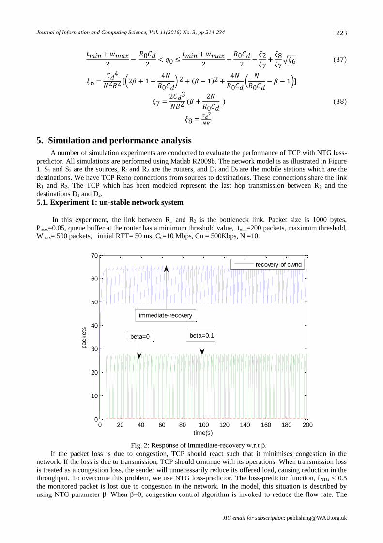
5.1. Experiment 1: un-stable network system
In this experiment, the link between R1 and R2 is the bottleneck link. Packet size is 1000 bytes,
Pmax=0.05, queue buffer at the router has a minimum threshold value, tmin=200 packets, maximum threshold,
Wmax= 500 packets, initial RTT= 50 ms, Cd=10 Mbps, Cu = 500Kbps, N =10.
Fig. 2: Response of immediate-recovery w.r.t β.
If the packet loss is due to congestion, TCP should react such that it minimises congestion in the
network. If the loss is due to transmission, TCP should continue with its operations. When transmission loss
is treated as a congestion loss, the sender will unnecessarily reduce its offered load, causing reduction in the
throughput. To overcome this problem, we use NTG loss-predictor. The loss-predictor function, fNTG < 0.5
the monitored packet is lost due to congestion in the network. In the model, this situation is described by
using NTG parameter β. When β=0, congestion control algorithm is invoked to reduce the flow rate. The
0 20 40 60 80 100 120 140 160 180 2000
10
20
30
40
50
60
70
time(s)
packets
recovery of cwnd
beta=0 beta=0.1
immediate-recovery

N.G.Goudru et al.: Enhancement of Performance of TCP Using Normalised Throughput Gradient in Wireless Networks
JIC email for contribution: [email protected]
224
loss-predictor function, fNTG ≥ 0.5 the monitored packet is lost due to wireless transmission then β=0.1
(conveniently selected value) immediate-recovery algorithms is invoked. The advantage of introducing β is
within a short span of time the sender window size recovered from one packet to the window size whose
flow rate was that of previous rtt. The graph in fig.2 illustrates the traces of immediate-recovery algorithm
when fNTG ≥ 0.5.
5.1.1. Analysis of performance metrics of fNTG
This experiment was conducted to analyse the performance ability of NTG loss-predictor to distinguish
congestion loss from wireless transmission loss. Important performance analysis metrics are, (i) Frequency
of congestion loss prediction (FCP): FCP is obtained by dividing the number of times the loss-predictor
predicts that the next loss will be due to congestion, by the total number of times the predictor was evaluated
during the TCP connection. Two counters are introduced to count the number of times the congestion and the
transmission losses accrues. The estimated values were used in the calculation of FCP, FWP, Ac and Aw. In
this experiment, number of times the NTG loss-predictor predicts that the next loss will be due to
congestion=812. Total number of times the predictor is evaluated during a TCP connection=2000.
FCP=812/2000=0.406(approximately 40%). (ii) Frequency of wireless loss prediction (FWP): FWP is
obtained by dividing the number of times the NTG loss-predictor predicts that the next loss will be due to
wireless transmission error, by the total number of times the predictor was evaluated during the TCP
connection. Number of times the loss-predictor is predicted that the next loss will be due to wireless=1188.
Total number of times the predictor is evaluated during a TCP connection=2000. FWP= 1188 /2000=0.594
(approximately 60%). (iii) Congestion loss prediction (Ac): Ac is the fraction of packet losses due to
congestion, diagnosed by NTG loss-predictor. (iv) Wireless loss prediction (Aw): Aw is the fraction of
packet losses due to wireless transmission errors diagnosed by NTG loss-predictor.
Fig. 3: Variation of FCP, FWP, Ac and Aw w.r.t time.
In experiment 1, during the simulation, approximately 40% of the losses are due to congestion and 60%
of the losses are due to wireless transmission as predicted by the loss-predictor. The graph of Fig. 3 shows
the performance metric with respect to (w.r.t) time in seconds.
0 20 40 60 80 100 120 140 160 180 20010
-4
10-3
10-2
10-1
100
time(s)
FCP
FWP
Ac
Aw
FWP
Ac
Aw
FCP

Journal of Information and Computing Science, Vol. 11(2016) No. 3, pp 214-234
JIC email for subscription: [email protected]
225
Fig. 4: Rtt-delay versus FCP and AC.
The round trip time (RTT) is the total time taken by a packet to travel from source to destination and the
ACK from destination to source. In our work, RTT includes variable queuing delay and a constant
propagation delay. In the experiment, we assume that both wired and wireless medium has a constant
propagation delay of 50 ms. Thus, RTT varies over the range [50, 250] milliseconds. Since RTT depends on
queue length, we observe that increase in queue length leads to increase in RTT value and vice versa. Larger
the queue length implies higher the congestion. Fig.4 describe the performance of FCP and Ac. FCP increase
slowly in the beginning and becomes high over the RTT range 200 to 250 . Increase in congestion is
responsible for increase in FCP. The graph is also associated with the fraction of packet losses due to
congestion diagnosed by NTG loss-predictor. Fig.5 illustrates the traces of FWP and Aw with respect to rtt-
delay. FWP is almost constant till rtt-delay reach 220 ms, suddenly increases when delay is 220-245 ms. This
may be because of burst in traffic and wireless transmission impairments. The graph is also associated with
Aw, the fraction of packet losses due to wireless transmission errors diagnosed by NTG loss-predictor.
Queue length is measured at the bottleneck link of R2. We consider a variable queue which depends on
the components such as (i) traffic due to arrival of the packets from TCP- sources,(ii) decrease in queue
length due to servicing of the packets by the router and delay of the packet departure. NTG loss-predictor
built based on congestion avoidance strategy, so fNTG is increasing with increase in queue length. As a result,
FCP increases slowly in the beginning and high with the increase queuing-delay. The traces of Fig. 6 and Fig.
7 illustrate the variation of FCP, FWP, Ac and Aw w.r.t queuing-delay. Sum of the fraction of packet losses
due to congestion (Ac) is 11 packets and sum of the fraction of packet losses due to transmission (Aw) is 7
packets for a total of 119520 packets transported during simulation.
0 50 100 150 200 25010
-4
10-3
10-2
10-1
100
rtt(ms)
FCP
AC
FCP
AC

N.G.Goudru et al.: Enhancement of Performance of TCP Using Normalised Throughput Gradient in Wireless Networks
JIC email for contribution: [email protected]
226
Fig.5: rtt-delay versus FWP and AW.
Fig.6: queuing-delay versus FCP and Ac.
0 50 100 150 200 25010
-4
10-3
10-2
10-1
100
rtt(s)
FWP
AW
FWP
AW
-0.05 0 0.05 0.1 0.15 0.20
0.1
0.2
0.3
0.4
0.5
0.6
0.7
0.8
0.9
1
queuing-delay(s)
FCP
Ac
Ac
FCP

Journal of Information and Computing Science, Vol. 11(2016) No. 3, pp 214-234
JIC email for subscription: [email protected]
227
Fig.7: queuing-delay versus FWP and AW.
5.2. Experiment 2: stable network system
The objective of stability analysis is to minimise the occurrence of queue overflow and underflow, thus
reducing the packet loss and maximising the link utilisation. Majority of the end-point control techniques
regulate the traffic demands according to the resources available in the wireless network. In an end-to-end
control scheme, stability analysis can achieve optimality. A time-delay control theory is applied for the
analysis of FCP, Ac, FWP, and Aw. Knowing the wireless network parameters such as Cd, Cu, N, R0 (round
trip time), and B (RED parameter, determined by maximum minus minimum queue buffer threshold values).
we derive a stability range for Pmax(maximum packet dropping probability) and β (fNTG parameter for
immediate- recovery). The relations are illustrated in equation (19) and (20) with reference to theorem-1.
Given, Cd=10Mbps, Cu=500Kbps, B=300packets, N=10, R0=100 ms, at the equilibrium point we get
Pmax=0.0068, and β=0.1538.
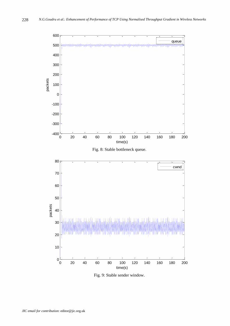
The graphs in Fig.8 and Fig. 9 describe the stable queue length and sender window size respectively
with respect to time. Queue length in the bottleneck link fluctuates over the range of [498, 500] packets. The
sender window fluctuates over the range of [26, 29] packets. Since queue length stabilises over a definite
range based on the available resources, the packet losses due to congestion is very small. The packet losses
due to wireless transmission remain unchanged. The traces of Fig. 10 illustrate congestion and wireless
losses with respect to time. Fig. 11 presents the immediate- recovery of the sender window size when the
loss predictor predicts that next packet loss is due to transmission.
-0.05 0 0.05 0.1 0.15 0.20
0.1
0.2
0.3
0.4
0.5
0.6
0.7
0.8
0.9
1
queuing-delay(s)
FWP
Aw
FWP
Aw
N.G.Goudru et al.: Enhancement of Performance of TCP Using Normalised Throughput Gradient in Wireless Networks
JIC email for contribution: [email protected]
228
Fig. 8: Stable bottleneck queue.
Fig. 9: Stable sender window.
0 20 40 60 80 100 120 140 160 180 200-400
-300
-200
-100
0
100
200
300
400
500
600
time(s)
packets
queue
0 20 40 60 80 100 120 140 160 180 2000
10
20
30
40
50
60
70
80
time(s)
packets
cwnd

Journal of Information and Computing Science, Vol. 11(2016) No. 3, pp 214-234
JIC email for subscription: [email protected]
229
Fig.10: Stable congestion-loss and wireless-loss
Fig. 11:Stable immediate-recovery of source w.r.t fNTG
0 20 40 60 80 100 120 140 160 180 20010
-2
10-1
100
101
102
time(s)
packets
C-loss
W-loss
wireless-loss
congestion-loss
0 20 40 60 80 100 120 140 160 180 20010
-1
100
101
102
103
time(s)
packets
immediate-recovery
beta
immediate-recovery
sender-window

N.G.Goudru et al.: Enhancement of Performance of TCP Using Normalised Throughput Gradient in Wireless Networks
JIC email for contribution: [email protected]
230
Fig.12: FCP and Ac w.r.t. time.
Fig. 13: FWP and Aw w.r.t. time.
Number of times the loss predictor predicted that the next loss is due to congestion= 652.Total number
of times the predictor evaluated during a TCP connection=2000. FCP=605/2000=0.3025 (approximately
30%). Number of times the loss predictor predicted that the next loss is due to wireless=1394. Total number
of times the predictor evaluated during a TCP connection=2000. FWP=1395/2000= 0.6975 (approximately
70%). Figure 12 and Fig. 13 illustrate the NTG prediction of congestion loss and transmission losses
0 20 40 60 80 100 120 140 160 180 20010
-6
10-5
10-4
10-3
10-2
10-1
100
time(s)
FCP
AC
FCPAc
0 20 40 60 80 100 120 140 160 180 20010
-4
10-3
10-2
10-1
100
time(s)
FWP
AW
FWP
AW
Journal of Information and Computing Science, Vol. 11(2016) No. 3, pp 214-234
JIC email for subscription: [email protected]
231
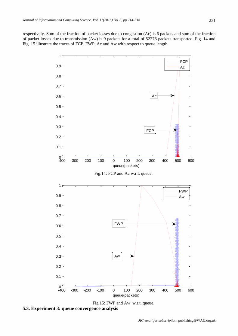
respectively. Sum of the fraction of packet losses due to congestion (Ac) is 6 packets and sum of the fraction
of packet losses due to transmission (Aw) is 9 packets for a total of 52276 packets transported. Fig. 14 and
Fig. 15 illustrate the traces of FCP, FWP, Ac and Aw with respect to queue length.
Fig.14: FCP and Ac w.r.t. queue.
Fig.15: FWP and Aw w.r.t. queue.
5.3. Experiment 3: queue convergence analysis
-400 -300 -200 -100 0 100 200 300 400 500 6000
0.1
0.2
0.3
0.4
0.5
0.6
0.7
0.8
0.9
1
queue(packets)
FCP
Ac
FCP
Ac
-400 -300 -200 -100 0 100 200 300 400 500 6000
0.1
0.2
0.3
0.4
0.5
0.6
0.7
0.8
0.9
1
queue(packets)
FWP
Aw
Aw
FWP

N.G.Goudru et al.: Enhancement of Performance of TCP Using Normalised Throughput Gradient in Wireless Networks
JIC email for contribution: [email protected]
232
In a bust traffic, sender window and queue length exhibit oscillatory behaviour. The objective of
analysis of convergence of the queue length is to minimise oscillatory nature of RED router. Using q0 as the
initial value, queue length converges faster to the given target value. This helps in improving the fairness of
the system. Knowing the wireless network parameters Cd , Cu, N, R0, and B, we derive a range of
convergence for Pmax, β, and q0 using the relations (34),(35) and (37). Using (37) estimate q0, by using this
value of q0 and (34) find pmax, by using pmax and (35) find β. Given Cd=4Mbps, Cu=500Kbps, tmin= 200
packets, wmax= 500 packets, N=10, R0=100 ms, B=300 packets, taget value, T=350 packets, we get, q0=313,
Pmax=0.0054, and β=0.0018. The range of convergence of queue length is (305.12, 320.8). The traces of the
graph of Fig. 16 illustrate the convergence of queue length for a given target value.
Maximum duration of the simulation time, the value of loss-predictor function fNTG is greater than 0.5,
predicting FCP is negligible and Ac is near to zero. Majority of the predictions are wireless transmission
losses. The traces of Fig. 17 and Fig.18 describe the performance of fNTG when queue convergence scheme is
deployed.
Fig.16: Queue convergence to target value=350 packets.
6. Conclusion
The work presented in this paper is a novel research to improve the performance of TCP in wireless
networks. The proposed transport model gives and end-to-end solution. The main problem of TCP has an
implicit assumption that all packet loss is due to congestion which is resolved by introducing NTG loss-
predictor. The NTG loss-predictor is a congestion avoidance method. NTG loss-predictor parameter β is
integrated with the system model, and can tune depending on the prediction of the losses. Statistical analysis
of FCP,FWP, Ac and Aw are made. After a successful implementation of loss detection in TCP, we tried to
minimise the packet loss due to congestion by introducing the concept of stability. The stability boundary of
two important tuning parameter Pmax and β is derived in terms wireless network parameters. Knowing the
wireless network resources and tuning these parameters, the system becomes asymptotically stable. After
successful control on congestion loss, we discuss convergence analysis of queue length at the ingress point of
the router. Condition for queue length convergence at the router is established. This helps in resolving the
oscillatory problem of RED router. Thus, the model presented in this work is efficient, fair and adaptable to
the wireless environment.
0 20 40 60 80 100 120 140 160 180 200100
150
200
250
300
350
400
450
500
550
time(s)
queue (
Packets
)
q(t) of a stable REDmaximum threshold
minimum hreshold
q0=313

Journal of Information and Computing Science, Vol. 11(2016) No. 3, pp 214-234
JIC email for subscription: [email protected]
233
Fig.17: Performance of FCP and Ac.
Fig.18: Performance of FWC and Aw.
7. References
Kai Xu, Ye Tian, and Nirwan Ansari,” TCP-Jersey for Wireless IP Communications”, IEEE journal on selected
areas in communications, 22( 4)( 2004).
0 20 40 60 80 100 120 140 160 180 2000
1
2
3
4
5
6x 10
-4
time(s)
FCP
Ac
Ac
FCP
0 20 40 60 80 100 120 140 160 180 20010
-6
10-5
10-4
10-3
10-2
10-1
100
time(s)
FWP
AwFWP
Aw

N.G.Goudru et al.: Enhancement of Performance of TCP Using Normalised Throughput Gradient in Wireless Networks
JIC email for contribution: [email protected]
234
Sally Floyd and Van Jacobson,” Random Early Detection Gateways for Congestion Avoidance”, IEEE/ACM
Transactions on Networking,(1993).
Francois Baccelli & Ki Baek Kim,”TCP Throughput Analysis under Transmission Error and Congestion Losses”,
IEEE INFOCOM, 0-7803-8356-7, (2004).
A. Bakre and B. R. Badrinath, “I-TCP: Indirect TCP for Mobile Hosts”, Proceedings of 15th International Conf.
on Distributed Computing Systems (ICDCS), (1995).
K. Brown and S. Singh, “M-TCP: TCP for Mobile Cellular Networks”, In Proceedings of INFOCOM ’96, (1996).
H. Balakrishnan, S. Seshan, E. Amir and R. H. katz., “Improving TCP/IP Performance over Wireless Networks”,
In Proceedings of ACM MOBICOM ’95, (1995).
H. Balakrishnan and R. H. Katz, “Explicit Loss Notification and Wireless Web Performance”, In Proceedings of
IEEE GLOBECOM ’98, (1998).
P. Sinha et al.(1999), “WTCP: A Reliable Transport Protocol for Wireless Wide-Area Networks”, In Proceedings
of ACM MOBICOM, (1999).
S. Mascolo and C. Casetti, “TCP Westwood: Bandwidth Estimation for Enhanced Transport over Wireless Links”,
In Proceedings of MOBICOM ’,(2001).
Seongho Cho, and Heekyoung Woo, ‘’TCP Performance Improvement with ACK Pacing in Wireless Data
Networks”, School of Electrical Engineering and Computer Science, Seoul National University, Seoul, Republic
of Korea, (2005).
Eric Hsiao-Kuang Wu, and Mei-Zhen Chen,” JTCP: Jitter-based TCP for heterogeneous wireless networks”, IEEE
journal on selected areas in communications, 22(4)( 2004).
Masashi Nakata, Go Hasegawa, Hirotaka Nakano, “Modeling TCP throughput over wired/wireless heterogeneous
networks for receiver-based splitting mechanism”, Graduate school of Information Science and Technology,
Osaka University, Japan.
Wei Zhang, Liansheng Tan, and Gang Peng, “ Dynamic queue level control for TCP/RED systems in AQM
routers”, Computers and Electrical Engineering, 35(2009)59-70.
Liansheng Tan, Wei Zhang, Gang Peng and Guanrong Chen, “ Stability of TCP/RED system in AQM routers”,
IEEE Transactions on automatic control, 51( 8) (2006).
L.Tan, W.Zhang, G.Peng and G.Chen, ”Stability of TCP/RED systems in AQM routers”, IEEE Trans. Automatic
control, 51(8)(2006) 1393-1398.
W.Zhang. L.Tan, and G.Peng, “Dynamic queue level control of TCP/RED systems in AQM routers”, Computers
and Electrical Engineering, 35(1)( 2009)59-70.
Hiroaki Mukaidani, Lin Cai, Xuemin Shen, “Stable queue management for supporting TCP flows over wireless
networks”, IEEE ICC, 978-1-61284-231-8/11, 2011.
Saad Biaz, and Nitin H.Vaidya, “Sender-based heuristics for distinguishing congestion losses from wireless
transmission losses”, Department of Computer Science, Texas Aand M University, USA, (2003).
Z.Wang, and J.Crowcroft,”A new congestion control scheme: Slow start and search (tri-s)”, ACM Computer
communication Review, 21(1991)32-43.
Anurag Kumar, D.majunath, Joy Kuri, “Communication Networking, an analytical approach”, Morgan Kaufmann
publisher an imprint of ELSEVIER, (2005).
Raj Jain, “A delay-based approach for congestion avoidance in interconnected heterogeneous computer networks”,
Digital equipment corporation, 550 king street, Littleton, MA-01460, (1989).
Ling-Yan Lu and Yi-Gang Cen, “Stability analysis of cooperative congestion control algorithm”, Tamkang
Journal of Science and Engineering, 14( 3)(2011)181-190.


![Linux 2.4 Implementation of Westwood+ TCP with rate-halving ...in the Internet [14]. To test and compare the Linux 2.4.19 implementations of Westwood+ and New Reno TCP more than 4000](https://img.pdfslide.us/doc/110x75/603f267fae920e61530e50f4/linux-24-implementation-of-westwood-tcp-with-rate-halving-in-the-internet.jpg)