Embed Size (px)
Citation preview
Experimental Testing of a Computer Aided Heat Treatment Planning
System
A
Thesis
Submitted to the faculty
of the
Worcester Polytechnic Institute
in partial fulfillment of the requirements for the
Degree of Master of Science
in
Mechanical Engineering
By
Rohit S.Vaidya
26 August 2003
Prof. Kevin Rong, (Major Advisor) Prof. Diran Apelian, Thesis Committee
Prof.R .D. Sisson.Jr, Thesis Committee Prof. J .M. Sullivan, Graduate Committee
ABSTRACT
Heat treatment is an important manufacturing process, which controls the mechanical
property of metal parts, therefore contributes to the product quality. A Computerized
Heat Treatment (CHT) system has been developed to model and simulate the heat
transfer in furnace. When the part load and thermal schedule information is given with
part and furnace specifications, the temperature profiles of parts in furnace can be
calculated based on heat transfer principle. Therefore the part load and thermal schedule
can be optimized to remove unnecessary delay time while the quality of heat treatment is
ensured.
In the thesis, the functions of CHT are enhanced with the capability of modeling and
simulating the heat treatment processes with random part load and continuous furnaces.
Methods to model random load and continuous furnace have been developed. Case
studies with industry real data have been conducted to validate the system and to show
effectiveness of the system. The system development is also introduced in the thesis.
ii

ACKNOWLEDGEMENT
I would like to express my gratitude to Prof. Kevin Rong, my advisor, for helping,
guiding and encouraging me to complete this thesis. I also thank Prof Apelian and Prof.
Richard Sisson for their enthusiastic service on the thesis committee.
I would like to thank MPI (CHTE) for providing me assistantship position in the
CHTE group. I would like to thank Larry Roether, General Manager of American Heat
Treating Inc for giving me an opportunity to work in their company and necessary help
whenever required. I would like thank my research group member Dr. Jinwu Kang for
providing technical knowledge and valuable advice whenever I needed during my
research work I would like to thank Bodycote Thermal processing plant, Worcester, MA
for allowing me to conduct case study in their company. I would like to thank my entire
group members in the Computer Aided Manufacturing Lab for their help during my
research work. . I would also like to thank the program secretary, Ms. Barbara Edilberti,
for helping me out during my stay at WPI
I would like to thank my family for supporting me throughout, during my study in
WPI. I would also like to thank my friends for helping me out during my study in WPI.
iii
TABLE OF CONTENTS Page
ABSTRACT ……………………………………………………………. ii
ACKNOWLEDGEMENT ……………………………………………… iii
TABLE OF CONTENTS ………………………………………………. iv
LIST OF FIGURES …………………………………………………….. vi
LIST OF TABLES ……………………………………………………... ix
CHAPTER 1. INTRODUCTION AND SYSTEMS REVIEW ……….. 1
1.1 Heat Treatment Processes
1.2 Problem Description
1.3 Research Objectives
CHAPTER 2. HEAT TRANSFER PRINCIPLE …….………………… 5
2.1 Heat Transfer Principle
2.2 Previous Research
2.3 Thesis Focus
CHAPTER 3. RANDOM LOAD PATTERN …………………………. 12
3.1 Random Load Pattern
3.2 Review Studies on Random Arrangements
3.3 Mathematical Model for Heat Transfer in Random Loads
3.4 Conclusion
CHAPTER 4. CASE STUDY FOR RANDOM LOAD PATTERN ….. 30
4.1 Case Study 1
4.2 Case Study 2
4.3 Conclusion
iv
CHAPTER 5. CONTINOUS FURNACE MODELING……………….. 40
5.1 Background of Heat Treatment in Continuous Furnaces
5.2 Classification of Continuous Furnaces
5.3 Studies about Continuous Furnaces
5.4 Problem Formulation of Heat Transfer in Continuous Furnace
5.5 Mathematical Model for Heat Transfer in Continuous Furnace
5.6 Numerical Calculation
5.7 Heat Balance
5.8 Random Load Patterns
5.9 Output Results and Optimization of Furnace Control
5.10 Summary
CHAPTER 6. SYSTEM DESIGN……………………………………… 64
6.1 System Structure
6.2 Database Design for Continuous Furnaces
6.3 System Interface Design
CHAPTER 7. CASE STUDY FOR CONTINUOUS FURNACE……… 79
7.1 Furnace Specifications
7.2 Workpiece Specification
7.3 Calculation
7.4 Results & Conclusion
CHAPTER.8 SUMMARY…………………………………………… 84
REFERENCE………………………………………………………… 85
v
LIST OF FIGURES
Page
1. Flow chart showing various modules of the CHT- bf system 9
2. Random load pattern examples 12
3. The influence of porosity on thermal conductivity 14
4. Enmeshment of contact sphere with different strain ratio 15
5. Normalized thermal resistance as a function of normalized contact 15
6. An example of the configuration of completely packed rods 16
7. Random package of mono-sized tetrahedral and multi-sized
tetrahedral
17
8. Random load pattern examples 17
9. Random load pattern software 18
10. Flowchart of effective thermal conductivity method 19
11. The specially designed load sample 20
12. Real load samples 22
13. Flowchart of effective thermal conductivity method based on
measured results
23
14. Random load pattern model 25
15. Enmeshment of random load pattern 25
16. Comparison of radiation and conduction between contact spheres 27
17. Comparison of radiation and conduction between cylinders 28
18. Casco workpieces 30
19. Gas fired Furnace 31
20. Load Pattern 32
21. Arrangement of the thermocouples 33
22. Comparison of calculated and measured results 34
23. Workpiece shape and size 35
24. Vacuum furnace 36
25. Load pattern and arrangement 37
vi
26. Graph showing measured and calculated values 38
27. A rotary-hearth furnace 41
28. A schematic view of tray movement in a pusher furnace 42
29. The load pattern for continuous belt in FurnXpert software 43
30. The result illustration of FurnXpert software 43
31. Schematic showing the various modes of heat transfer in a
continuous reheating furnace
44
32. The individual control volumes used to discretized the one-
dimensional continuous heating furnace model
44
33. The heating of strip 45
34. Continuous furnace model 48-49
35. Virtual fixture size definition for continuous movement 53
36. Relationship between temperature-time curve and temperature-
distance curve for step by step movement
57
37. Heat loss terms 58
38. The effects of moving speed on thermal schedule of continuous
furnace
62-63
39. Users perspective for CHT-cf 64
40. Sequence chart for CHT-cf 65
41. Flowchart for continuous furnace 66
42. System architecture 67
43. Continuous furnace database structure 68
44. Workpiece definition 1 69
45. Workpiece definition 2 70
46. Workpiece definition 3 70
47. Virtual fixture size definition for continuous furnace 71
48. Continuous furnace definition 1 72
vii
49. Continuous furnace definition 2 72
50. Continuous furnace definition 3 73
51. Continuous furnace definition 4 73
52. Load pattern definition 74
53. Calculation page 75
54. Temperature-time profile result 76
55. Report 76
56. Database management 77
57. Continuous furnace database management 78
58. Shaker Furnace used for the Case Study 79
59. Workpieces on the furnace and its dimensions 80
60. The results obtained from system for the current case 82
61. Temperature curves obtained from system (Set point & Slowest
curves)
82
viii
LIST OF TABLES
Page
1. Workpiece definition for case 1 31
2. Furnace information 32
3. Load pattern for case 1 33
4. Workpiece data 35
5. Furnace data 36
6. Load pattern 37
7. Comparison of continuous furnaces and batch furnaces 46
8. Comparison of heat transfer in continuous furnaces and batch
furnaces
47
9. Furnace data 80
10. Workpiece data 81
11. Furnace temperature data 81
ix
CHAPTER 1. INTRODUCTION Heat Treatment is the controlled heating and cooling of metals to alter their physical and
mechanical properties without changing the product shape. Heat treatment is sometimes
done inadvertently due to manufacturing processes that either heat or cool the metal such
as welding or forming.
Heat Treatment is often associated with increasing the strength of material, but it can also
be used to alter certain manufacturability objectives such as to improve machinability and
formability, and to restore ductility after a cold working operation. Thus it is a very
enabling manufacturing process that can not only help other manufacturing processes, but
also improve product performance by increasing strength or other desirable
characteristics. Steels are particularly suitable for heat treatment, since they respond well
to heat treatment and the commercial use of steels exceeds that of any other materials.
1.1 Heat Treatment Processes The term heat-treatment embraces many processes employing combinations of heating
and cooling operations, applied to moulds and dies, tools and machine components so as
to produce desired mechanical properties, with attendant characteristics related to
particular types of 'in-service' applications. Steel is the most common metal being treated.
It accounts for more than 80% of all metals.
The various processes may be broadly classified as:
a. Hardening process is intended to produce through hardened structure by quench-
hardening. Hardening increases wear resistance and the strength of materials, and
provides toughness after. However, the hardening often results in turning the structure of
the work brittle. Besides, internal stress increases tremendously while machinability and
ductility of the metal decrease. Therefore, the hardening processes need to be well
studied and controlled.
b. Softening process is intended primarily to soften the material, such as annealing, and
remove stresses either inherent or consequent upon prior operations, but generally
resulting in a softer structure. The latter processes include stress relieving and process
annealing.
1
c. Toughening process is intended to produce a structure possesses good strength and
ductility in steels by means of normalizing. Improved machinability, grain structure
refinement, homogenization and modification of residual stresses are among the reasons
for which normalizing is done.
d. Case-hardening process is employed to produce a 'case' or surface layer substantially
harder than the interior or core of the workpiece. They include carburizing, nitriding and
induction hardening.
In this research, the heating process is studied. In order to perform a quality heat-
treatment, the heat source in a furnace is heated first by the electric or fired gas (indirect
or direct). The heat flux arrives at the surfaces of workpieces through radiation and
convection heat transfer and arises the surfaces temperature of the workpieces. Then the
temperature in the interior of a workpiece is raised in the form of conduction heat
transfer. Thus, the heat treatment of workpieces is such a process that the workpieces are
heated up with the radiation/convection hybrid boundary condition on the surfaces and
with the conduction heat transfer interiorly. The uniformity of temperature distribution
and the delay time of inside temperature will contribute to the material property control
and the heat treatment quality. To optimize the temperature control and load design, it is
necessary to study the detail information about the temperature distribution in furnace
and workpieces as a function of time.
1.2 Problem Description To optimize the heat treatment processes, three categories of problems need to be
considered. They are,
Quality control in the heat treatment
Productivity
Experience based process design and lack of a proper calculation tool.
Quality Control in the Heat Treatment
The quality control of heat treatment for metal parts depends on many factors, including
part load and furnace temperature control. It is desired to predict the heating history and
2
temperature distributions in furnace and in workpiece so that the part load design and
temperature control can be improved. Unfortunately, there is currently no comprehensive
technique, which can be used to simulate heat-treating process and predict the
temperature distribution of workpieces with arbitrary geometry in a loaded furnace. In
current practice in heat treating industry, to ensure the quality, experimental methods
have to be employed to measure the temperature in furnace space or on part surfaces.
Productivity
The term productivity can be directly related to two terms, one being the energy
consumption and the other being the cost involved in the production processes. As such
there is no direct measuring method for the inside-workpiece temperature measurement
in the heat-treating process. The temperature of workpieces may vary with time and
location, from surface to interior. Although the workpieces temperature may be measured
by thermocouples set on the workpieces surface at selected points, the interior
temperature of workpieces is still unknown, especially in the middle of the furnace. In
order to obtain a uniform temperature between the surface and the interior at different
furnace locations, a delay of time is necessary for heat transfer from outside the load to
inside the load, and heat conduction to the interior of the workpiece after the surface
temperature reached the specified temperature. Nowadays this time delay is determined
by experience because there is no analytical model available yet. The problem is, if the
holding time relatively short, the uniform temperature between the surface and the
interior cannot be obtained; but if it is too long, the mechanical property of the surface
material may be changed undesirably. The either way will result in the increase in the
cost involved in production, as the workpieces may have to be heat treated again.
Experience based process design and lack of a proper calculation tool.
The part load design and furnace temperature control in heat treating industry is based on
the experience for the majority of time. There are hardly any analytical tools in the heat
treating industry for the calculation of the thermal schedule as well as the workpiece
temperature. The most of calculations of thermal schedules are based on experience, as
well as the temperature reached by workpieces. Since there is no analytical model
3
available to predict the temperature distribution in workpieces, it is difficult to carry out
an optimization of the part load. The unreasonable part load may result in a non-
uniformity of temperature distributions in the workpiece. To obtain the temperature
distribution and heating history of workpiece, a comprehensive mathematical model
needs to be developed for the heat transfer process in heat treatment. The heat
conduction in workpiece can be modeled based on the well-known heat conduction
principle. The difficult is that the boundary condition is varying in time and locations of
the workpiece. The boundary condition is dominated by the convection and radiation in
furnace. How to integrate the related three heat transfer models into a comprehensive
model for heat treatment processes is the emphasis of the research. An effective
numerical method is also necessary for applying the model for solutions.
1.3. Research Objectives After studying the heat treatment processes and the current industrial practices. The
available systems for the processes was reviewed and found insufficient for the
requirements for the heat-treating industry. Hence the research objectives set were as
follows:
• To develop physics-mathematical models based on the heat transfer theory for the
various modes of heat transfer taking place between the furnace and the workpieces
and among the workpieces itself.
• To study and analyze the random load pattern of the workpieces and study their
effects and develop a database containing the above model parameters that are
properties of materials.
• To develop a user interface so as to obtain all the necessary data inputs or parameters
for the models.
• To validate and implement the system in the current industries.
4

CHAPTER 2. HEAT TRANSFER PRINCIPLE This chapter deals with the various heat treatment principles, which are divided into
conduction, convection and radiation. In this chapter we will briefly study the previous
research that have been done and present the scope of the research.
2.1 Heat Transfer Principle Heat is a form of energy and is transported from one body to another due to the
temperature differences in the bodies. The heat can transfer by one, or by a combination
of three separate modes known as conduction, convection and radiation. Conduction
occurs in a stationary medium; convection requires a moving medium; and radiation
occurs in absence of any medium, distinguishing it as part of electromagnetic spectrum.
Although they are distinct processes, they can occur together.
The heat generated in a diesel engine, for example, is transferred from the combusted gas
to the steel cylinder walls by the combined action of radiation and convection. Heat flows
through the cylinder walls by conduction. In turn, the outer surface of the wall is cooled
by convection, and so some extend radiation, owing to water circulating in the cooling
passages. The physical processes that govern conduction, convection and radiation are
quite different, leading to have a different approach for each process analysis.
2.1.1 Conduction heat transfer Conduction occurs in a stationary medium. It is most likely to be of concern in solids,
although conduction may present to some extent in gases and liquids. In the solids the
mechanism of conduction is due to the vibration of the atomic lattice and the motion of
the free electrons, the latter generally being a more powerful effect. The metallic solids
are good conductors because of the contribution made by available free electrons.
Conduction is governed by Fourier’s law, which states, “the rate of flow of heat through a
simple homogenous solid is directly proportional to the area of the section at right angles
to the direction of heat flow, and to change of temperature with respect to the length of
the path of the heat flow [1].
It is represented mathematically by the equation:
5

dxdtAQ α (1)
where Q = heat flow through a body per unit time (watts);
A = surface area of heat flow perpendicular to direction of flow (m2);
dt = temperature difference of the faces of body (homogenous solid) of thickness
dx’ through which heat flows, (°C or K); and
dx = thickness of body in the direction of flow (m).
Thus,
dxdtAQ .λ−= (2)
where λ = a constant of proportionality and known as thermal conductivity
The negative sign is to take care of the decreasing temperature along with the direction of
increasing thickness or the direction of the flow. The temperature gradient dt/dx is always
negative along positive x direction and, therefore the value of Q become positive.
2.1.2 Convection heat transfer Heat transfer due to medium in form of liquid or gas occurs in convection heat transfer.
The convection heat transfer equation between a surface and an adjacent medium is
prescribed by Newton’s law of cooling [1].
)( fs ttAhQ −= (3)
where, Q = rate of convective heat transfer (watts);
A = surface area exposed to heat transfer (m2);
ts = surface temperature (°C or K);
tf = fluid temperature (°C or K); and
h = coefficient of convection heat transfer (W/m2-K)
The coefficient of convection heat transfer ‘h’ is defined as “the amount of heat
transmitted for a unit temperature difference between the fluid and unit area of surface in
unit time”. The value of ‘h’ depends on thermodynamic properties (viscosity, density,
specific heat etc), nature of fluid flow, and geometry of the surface and prevailing
thermal conditions.
6
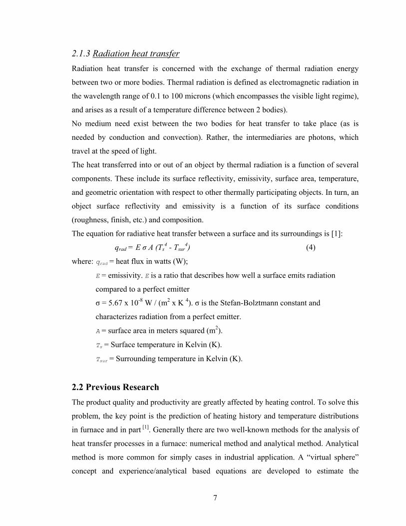
2.1.3 Radiation heat transfer Radiation heat transfer is concerned with the exchange of thermal radiation energy
between two or more bodies. Thermal radiation is defined as electromagnetic radiation in
the wavelength range of 0.1 to 100 microns (which encompasses the visible light regime),
and arises as a result of a temperature difference between 2 bodies).
No medium need exist between the two bodies for heat transfer to take place (as is
needed by conduction and convection). Rather, the intermediaries are photons, which
travel at the speed of light.
The heat transferred into or out of an object by thermal radiation is a function of several
components. These include its surface reflectivity, emissivity, surface area, temperature,
and geometric orientation with respect to other thermally participating objects. In turn, an
object surface reflectivity and emissivity is a function of its surface conditions
(roughness, finish, etc.) and composition.
The equation for radiative heat transfer between a surface and its surroundings is [1]: qrad = E σ A (Ts
4 - Tsur4) (4)
where: qrad = heat flux in watts (W);
E = emissivity. E is a ratio that describes how well a surface emits radiation
compared to a perfect emitter
σ = 5.67 x 10⁻⁸ W / (m2 x K 4). σ is the Stefan-Bolztmann constant and
characterizes radiation from a perfect emitter.
A = surface area in meters squared (m2).
Ts = Surface temperature in Kelvin (K).
Tsur = Surrounding temperature in Kelvin (K).
2.2 Previous Research The product quality and productivity are greatly affected by heating control. To solve this
problem, the key point is the prediction of heating history and temperature distributions
in furnace and in part [1]. Generally there are two well-known methods for the analysis of
heat transfer processes in a furnace: numerical method and analytical method. Analytical
method is more common for simply cases in industrial application. A “virtual sphere”
concept and experience/analytical based equations are developed to estimate the
7
equilibration time and heating rates in parts loaded in a furnace [2]. Analytical solutions
for the radiative heat transfer in box-shaped furnaces and cylindrical furnaces were
presented [3, 4]. A method of fitting general function form was used to estimate the
temperatures at the specified points in box-shaped and cylinder furnaces so as to replace
the temperature measurement. Both the part temperature and the furnace temperature
were predicted in ref. [5] without consideration of load patterns. These kinds of studies
can only deal with some regular shapes of parts without consideration of load patterns,
and the temperature distribution inside the parts is assumed uniform.
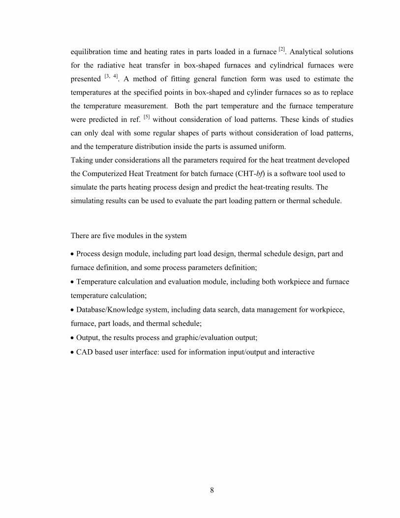
Taking under considerations all the parameters required for the heat treatment developed
the Computerized Heat Treatment for batch furnace (CHT-bf) is a software tool used to
simulate the parts heating process design and predict the heat-treating results. The
simulating results can be used to evaluate the part loading pattern or thermal schedule.
There are five modules in the system
• Process design module, including part load design, thermal schedule design, part and
furnace definition, and some process parameters definition;
• Temperature calculation and evaluation module, including both workpiece and furnace
temperature calculation;
• Database/Knowledge system, including data search, data management for workpiece,
furnace, part loads, and thermal schedule;
• Output, the results process and graphic/evaluation output;
• CAD based user interface: used for information input/output and interactive
8

Fur
Mat
Work
Temperature calculation
Process design
Thermal schedule design
Thermal schedule design
Part load design
Fig.1 Flow chart showing various
9
Furnace temperature calculation
piece database
Workpiece temperature calculation
Database structure
nace database
erial database
modules of the CHT-bf system
The system main functions include:
• The simulation of heating process of workpieces in loaded furnace;
• The calculation of the furnace average temperature for various types of furnaces;
• The calculation of energy balance for furnace heat-treating process;
• The design and optimization of the thermal schedule and part loading; and
• Database management system for heat-treat process design.
The objective of this research is to establish a knowledge-based computer-aided heat treat
planning software system for the heat treatment process optimization. The software was
basically designed by taking the arranged load pattern of the workpieces under
consideration, but in actual cases many times it was found that the load pattern to be
randomly placed. This leads to the addition of the random load model in the system.
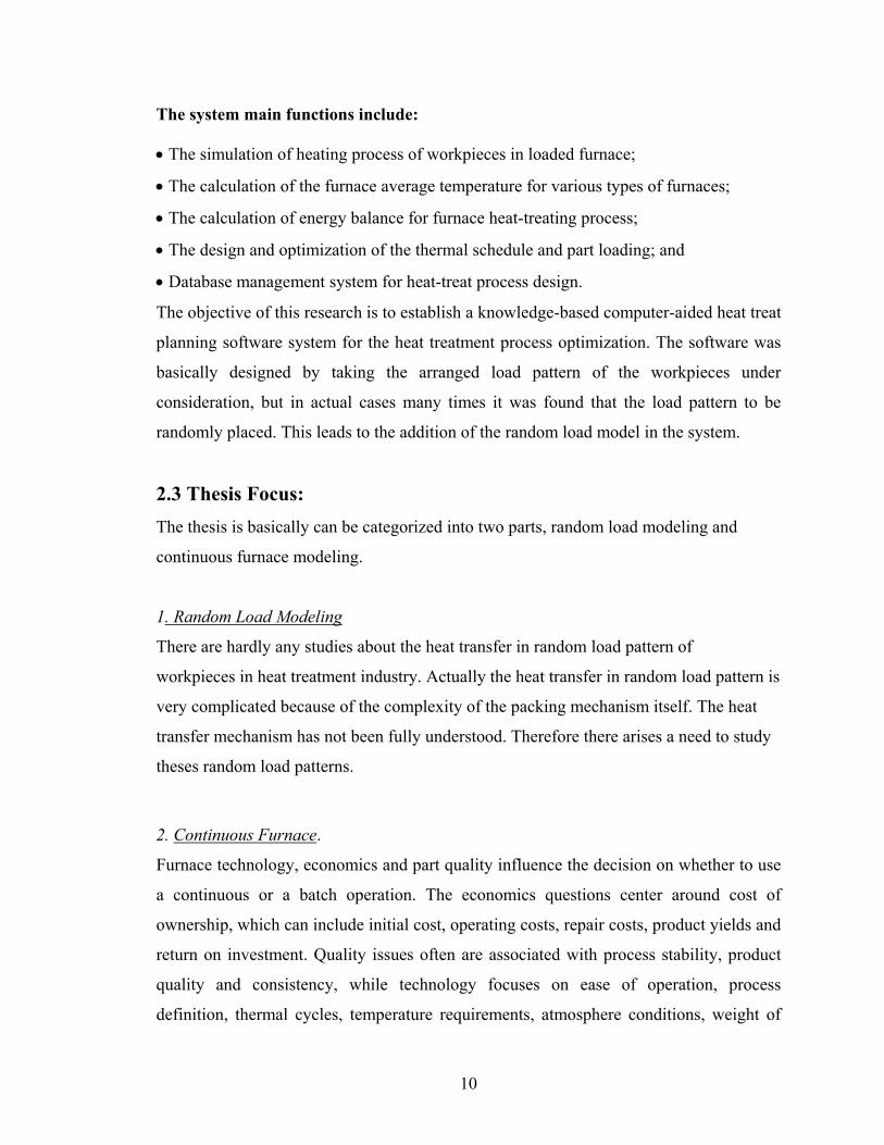
2.3 Thesis Focus: The thesis is basically can be categorized into two parts, random load modeling and
continuous furnace modeling.
1. Random Load Modeling
There are hardly any studies about the heat transfer in random load pattern of
workpieces in heat treatment industry. Actually the heat transfer in random load pattern is
very complicated because of the complexity of the packing mechanism itself. The heat
transfer mechanism has not been fully understood. Therefore there arises a need to study
theses random load patterns.
2. Continuous Furnace.
Furnace technology, economics and part quality influence the decision on whether to use
a continuous or a batch operation. The economics questions center around cost of
ownership, which can include initial cost, operating costs, repair costs, product yields and
return on investment. Quality issues often are associated with process stability, product
quality and consistency, while technology focuses on ease of operation, process
definition, thermal cycles, temperature requirements, atmosphere conditions, weight of
10

product and desired throughput. The questions and their relative importance vary from
industry to industry, company to company and person to person. But a universal set of
questions always concerns continuous furnace design. Thus the continuous furnaces more
or less are the part of almost every heat treatment industry. This leads to research and
develop an analytical tool for the calculation of temperature in the continuous furnace.
11
CHAPTER 3. RANDOM LOAD MODEL The Computerized Heat Treatment for batch furnace software (CHT-bf) was developed
with the view to study and predict the heat treatment process. The earlier version of
CHT-bf had more emphasis on the aligned load pattern, thus the next step was
considering the Random load pattern in the system. In this chapter, the heat transfer
problem of random load pattern was systemically reviewed and analyzed. Two practical
methods have been studied and applied to the system.
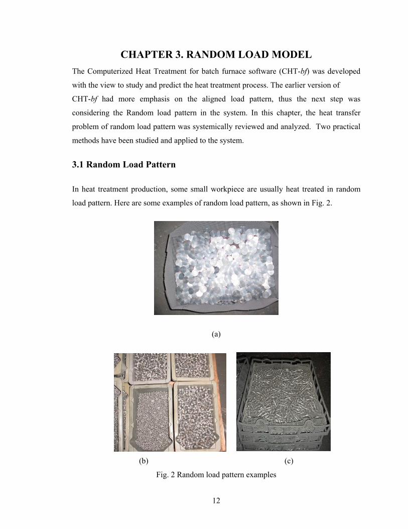
3.1 Random Load Pattern
In heat treatment production, some small workpiece are usually heat treated in random
load pattern. Here are some examples of random load pattern, as shown in Fig. 2.
(a)
(b) (c)
Fig. 2 Random load pattern examples
12

3.2 Review Studies on Random Arrangement
There are hardly any studies about the heat transfer in random load pattern of workpieces
in heat treating industry. Actually the heat transfer in random load pattern is very
complicated because of the complexity of the packing mechanism itself. The heat transfer
mechanism has not been fully understood. Here some related studies about random
packing of particles and the inside heat transfer are reviewed.
3.2.1 Conduction between small particles
The similar problem, the heat transfer in random packed particles, such as metal powder
in powder metallurgy, has been widely studied for a long time.
1) Thermal Conductivity in metal powder
To study the thermal conductivity of powder, equation for two-mixed phase was derived
by Maxwell as [2]
))(22)(2
(MDDMD
MDDMDMAg P
Pλλλλλλλλ
λλ−−+−++
= (5)
where Agλ , Mλ , Dλ are the thermal conductivities of the aggregate, matrix and disperse
phase, respectively, PD is the volume fraction of the disperse phase.
For powder, the matrix phase is air, so its thermal conductivity can be simplified as
follows,
)23
( −=APAp
λλ (6)
where pλ , Aλ are the thermal conductivity of the powder and air, respectively, PA is the
volume fraction of the air.
13
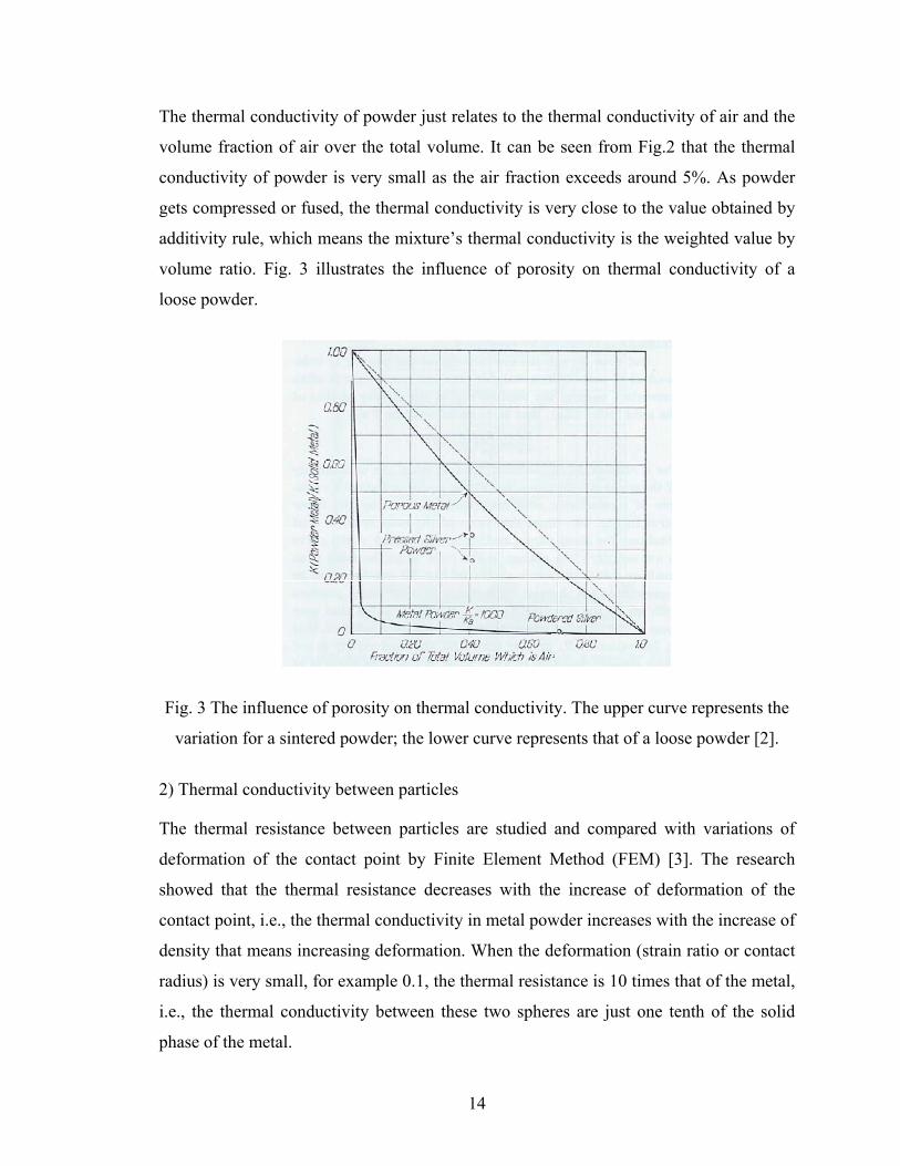
The thermal conductivity of powder just relates to the thermal conductivity of air and the
volume fraction of air over the total volume. It can be seen from Fig.2 that the thermal
conductivity of powder is very small as the air fraction exceeds around 5%. As powder
gets compressed or fused, the thermal conductivity is very close to the value obtained by
additivity rule, which means the mixture’s thermal conductivity is the weighted value by
volume ratio. Fig. 3 illustrates the influence of porosity on thermal conductivity of a
loose powder.
Fig. 3 The influence of porosity on thermal conductivity. The upper curve represents the
variation for a sintered powder; the lower curve represents that of a loose powder [2].
2) Thermal conductivity between particles
The thermal resistance between particles are studied and compared with variations of
deformation of the contact point by Finite Element Method (FEM) [3]. The research
showed that the thermal resistance decreases with the increase of deformation of the
contact point, i.e., the thermal conductivity in metal powder increases with the increase of
density that means increasing deformation. When the deformation (strain ratio or contact
radius) is very small, for example 0.1, the thermal resistance is 10 times that of the metal,
i.e., the thermal conductivity between these two spheres are just one tenth of the solid
phase of the metal.
14
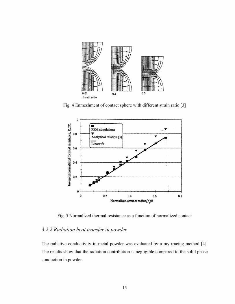
Fig. 4 Enmeshment of contact sphere with different strain ratio [3]
Fig. 5 Normalized thermal resistance as a function of normalized contact
3.2.2 Radiation heat transfer in powder
The radiative conductivity in metal powder was evaluated by a ray tracing method [4].
The results show that the radiation contribution is negligible compared to the solid phase
conduction in powder.
15

3.2.3 Construction of random load patterns
If the three-dimensional random load pattern model is constructed the heat transfer in
random load pattern can be solved by finite difference method (FDM) or FEM. Here
some studies about the construction of random load pattern are presented.
The study of particles packing is of industrial importance to determine the porosity in
geotechnical engineering of soils and rock fill, mining and mineral engineering, and in
powder technology. Because of complexity it is still limited to random packing of regular
shapes, such as cubic, sphere, rod, tetrahedral and etc. There are usually two kinds of
methods for random packing of particles, one is sequential algorithm (or Ballistic
deposition technique), and the other is collective algorithm (space filling). The first one is
that the particles are randomly dropped in the container one after another. Under the
influence of gravitational forces, the dropped particle will roll over the existing particles
until it reaches a stable position. The second one is that particles of zero size are first
randomly placed in the container. Following this initial distribution, sizes of the particles
are constantly increased. They are moved apart if overlap occurs between two particles
just in touch [5].
Fig. 6 An example of the configuration of completely packed rods (a=15) [6]
16
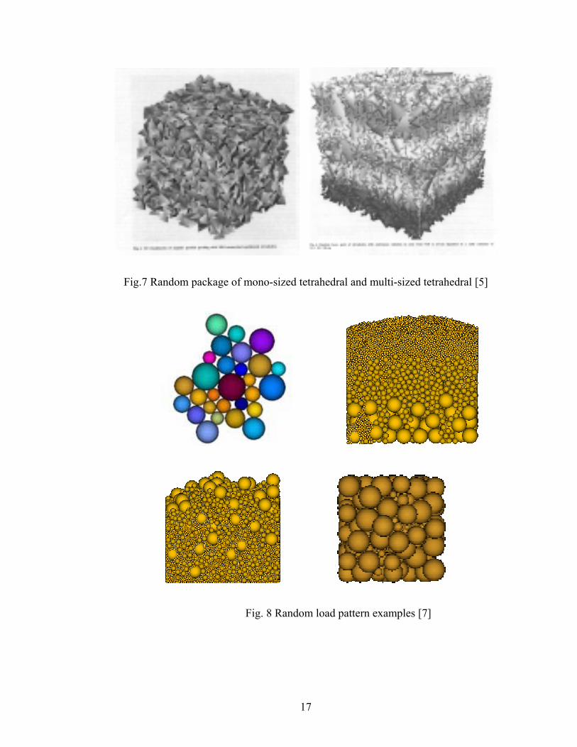
Fig.7 Random package of mono-sized tetrahedral and multi-sized tetrahedral [5]
Fig. 8 Random load pattern examples [7]
17
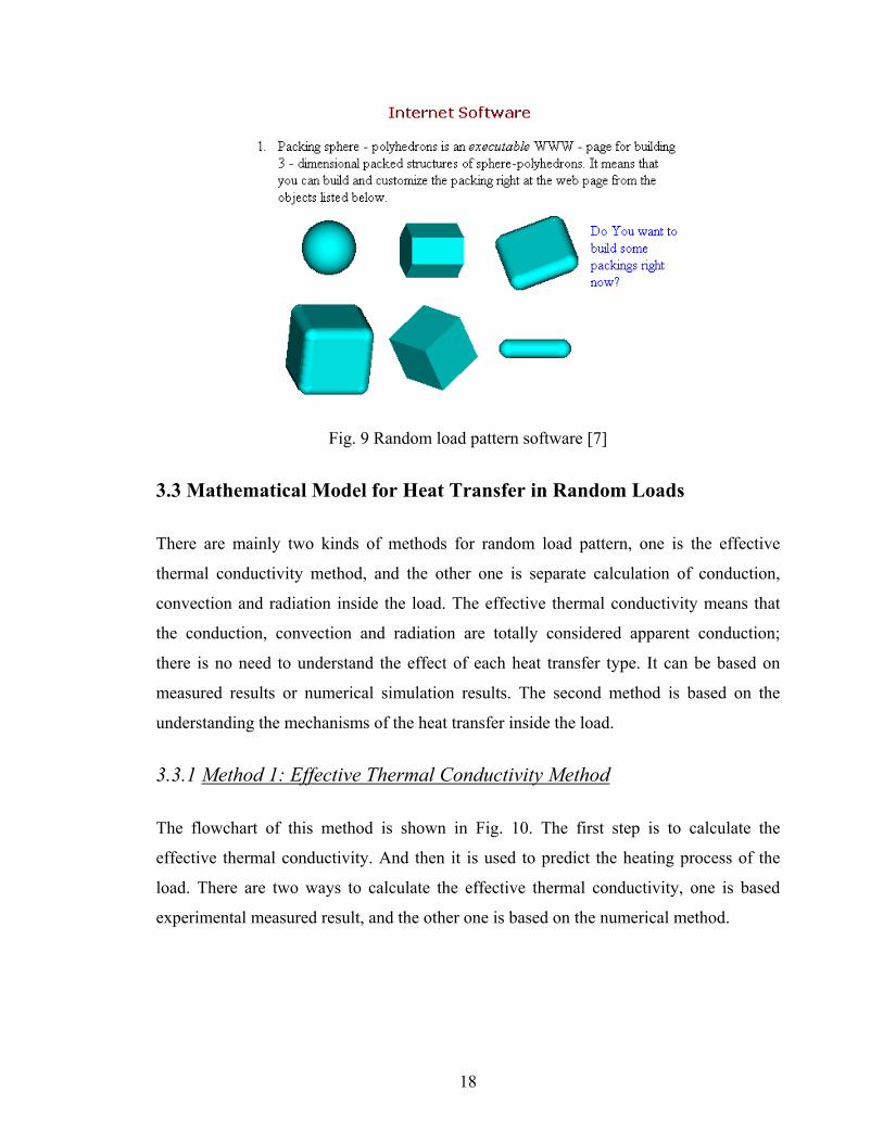
Fig. 9 Random load pattern software [7]
3.3 Mathematical Model for Heat Transfer in Random Loads
There are mainly two kinds of methods for random load pattern, one is the effective
thermal conductivity method, and the other one is separate calculation of conduction,
convection and radiation inside the load. The effective thermal conductivity means that
the conduction, convection and radiation are totally considered apparent conduction;
there is no need to understand the effect of each heat transfer type. It can be based on
measured results or numerical simulation results. The second method is based on the
understanding the mechanisms of the heat transfer inside the load.
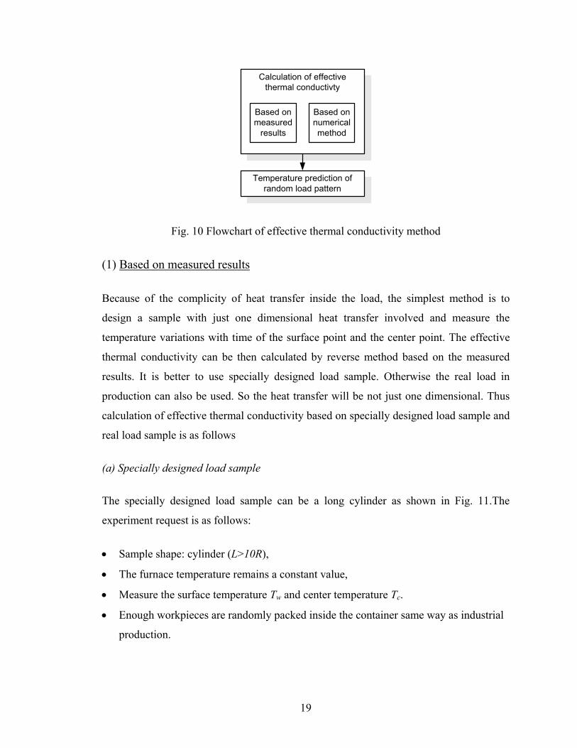
3.3.1 Method 1: Effective Thermal Conductivity Method
The flowchart of this method is shown in Fig. 10. The first step is to calculate the
effective thermal conductivity. And then it is used to predict the heating process of the
load. There are two ways to calculate the effective thermal conductivity, one is based
experimental measured result, and the other one is based on the numerical method.
18
Temperature prediction ofrandom load pattern
Calculation of effectivethermal conductivty
Based onmeasured
results
Based onnumericalmethod
Fig. 10 Flowchart of effective thermal conductivity method
(1) Based on measured results
Because of the complicity of heat transfer inside the load, the simplest method is to
design a sample with just one dimensional heat transfer involved and measure the
temperature variations with time of the surface point and the center point. The effective
thermal conductivity can be then calculated by reverse method based on the measured
results. It is better to use specially designed load sample. Otherwise the real load in
production can also be used. So the heat transfer will be not just one dimensional. Thus
calculation of effective thermal conductivity based on specially designed load sample and
real load sample is as follows
(a) Specially designed load sample
The specially designed load sample can be a long cylinder as shown in Fig. 11.The
experiment request is as follows:
• Sample shape: cylinder (L>10R),
• The furnace temperature remains a constant value,
• Measure the surface temperature Tw and center temperature Tc.
• Enough workpieces are randomly packed inside the container same way as industrial
production.
19
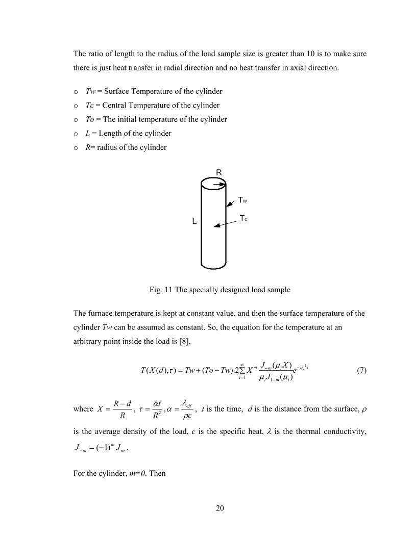
The ratio of length to the radius of the load sample size is greater than 10 is to make sure
there is just heat transfer in radial direction and no heat transfer in axial direction.
o Tw = Surface Temperature of the cylinder
o Tc = Central Temperature of the cylinder
o To = The initial temperature of the cylinder
o L = Length of the cylinder
o R= radius of the cylinder
R
L TC
TW
Fig. 11 The specially designed load sample
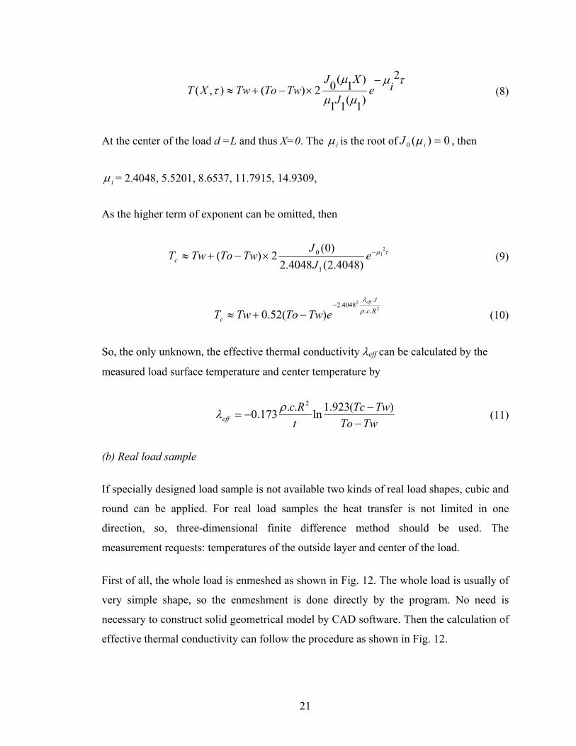
The furnace temperature is kept at constant value, and then the surface temperature of the
cylinder Tw can be assumed as constant. So, the equation for the temperature at an
arbitrary point inside the load is [8].
τµ
µµµτ
2
1 1 )()(2).()),(( ie
JXJXTwToTwdXT
i imi
imm −∞
= −
−∑−+= (7)
where R
dRX −= , 2R
tατ = ,c
eff
ρλ
α = , t is the time, d is the distance from the surface, ρ
is the average density of the load, c is the specific heat, λ is the thermal conductivity,
. mm
m JJ )1(−=−
For the cylinder, m=0. Then
20
τµ
µµ
µτ
2
)1(11
)1(02)(),( ieJ
XJTwToTwXT
−×−+≈ (8)
At the center of the load d =L and thus X=0. The iµ is the root of 0)(0 =iJ µ , then
iµ = 2.4048, 5.5201, 8.6537, 11.7915, 14.9309,
As the higher term of exponent can be omitted, then
τµ 21
)4048.2(4048.2)0(
2)(1
0 −×−+≈ eJ
JTwToTwTc (9)
22
..
.4048.2
)(52.0 Rc
t
c
eff
eTwToTwT ρ
λ−
−+≈ (10)
So, the only unknown, the effective thermal conductivity λeff can be calculated by the
measured load surface temperature and center temperature by
TwToTwTc
tRc
eff −−
−=)(923.1ln..173.0
2ρλ (11)
(b) Real load sample
If specially designed load sample is not available two kinds of real load shapes, cubic and
round can be applied. For real load samples the heat transfer is not limited in one
direction, so, three-dimensional finite difference method should be used. The
measurement requests: temperatures of the outside layer and center of the load.
First of all, the whole load is enmeshed as shown in Fig. 12. The whole load is usually of
very simple shape, so the enmeshment is done directly by the program. No need is
necessary to construct solid geometrical model by CAD software. Then the calculation of
effective thermal conductivity can follow the procedure as shown in Fig. 12.
21
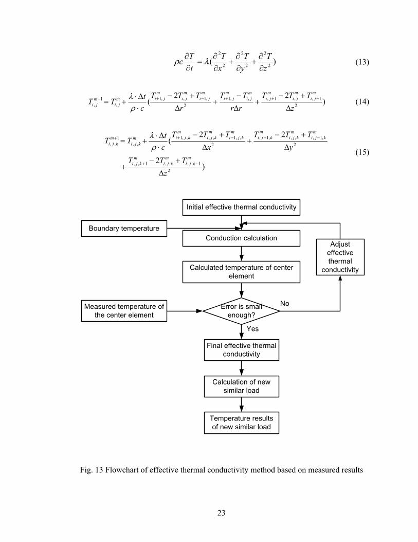
Firstly, give an initial value for effective thermal conductivity. Then calculate the
temperature of the center point by the measured temperatures of the outside layer as
boundary condition. Compare the calculated temperature and measured temperature of
the center point. If there is a great difference iterate the calculation with a new value for
thermal conductivity until the error falls into the reasonable range. And then the effective
thermal conductivity is obtained. Usually many iterations of calculation are necessary to
get the exact thermal conductivity. Here convection and radiation effects are also
included in the thermal conductivity.
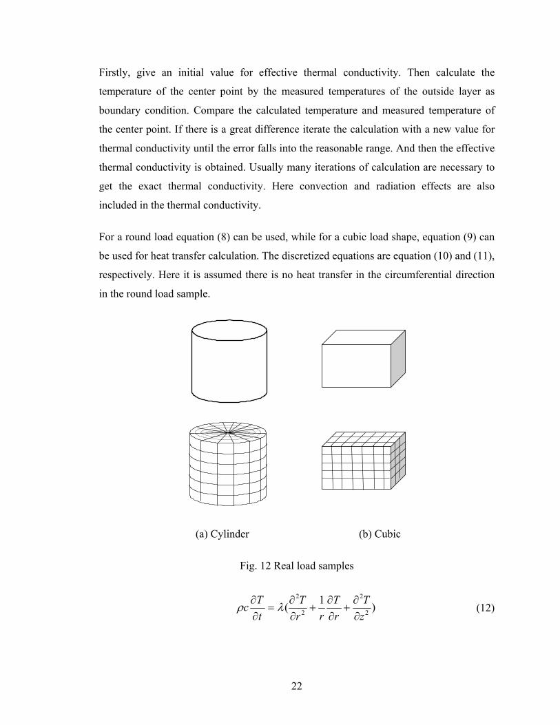
For a round load equation (8) can be used, while for a cubic load shape, equation (9) can
be used for heat transfer calculation. The discretized equations are equation (10) and (11),
respectively. Here it is assumed there is no heat transfer in the circumferential direction
in the round load sample.
(a) Cylinder (b) Cubic
Fig. 12 Real load samples
)1( 2
2
2
2
zT
rT
rrT
tTc
∂∂
+∂∂
+∂∂
=∂∂ λρ (12)
22
)( 2
2
2
2
2
2
zT
yT
xT
tTc
∂∂
+∂∂
+∂∂
=∂∂ λρ (13)
)22
( 21,,1,,,1
2,1,,1
,1
, zTTT
rrTT
rTTT
ctTT
mji
mji
mji
mji
mji
mji
mji
mjim
jimji ∆
+−+
∆
−+
∆
+−
⋅∆⋅
+= −++−++
ρλ (14)
)2
22(
21,,,,1,,
2,1,,,,1,
2,,1,,,,1
,,1
,,
zTTT
yTTT
xTTT
ctTT
mkji
mkji
mkji
mkji
mkji
mkji
mkji
mkji
mkjim
kjim
kji
∆
+−+
∆
+−+
∆
+−
⋅∆⋅
+=
−+
−+−++
ρλ
(15)
Adjusteffectivethermal
conductivity
Conduction calculation
Calculated temperature of centerelement
Measured temperature ofthe center element
Boundary temperature
Error is smallenough?
Initial effective thermal conductivity
Final effective thermalconductivity
Calculation of newsimilar load
Temperature resultsof new similar load
Yes
No
Fig. 13 Flowchart of effective thermal conductivity method based on measured results
23
(2) Based on numerical method
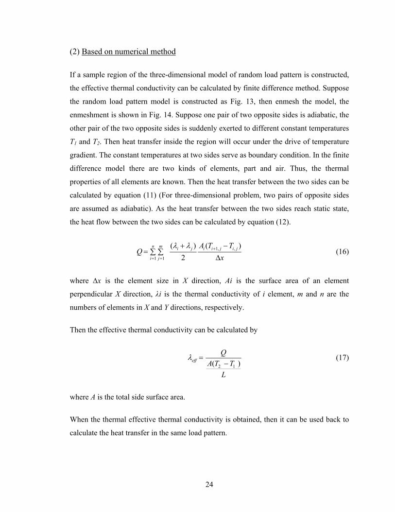
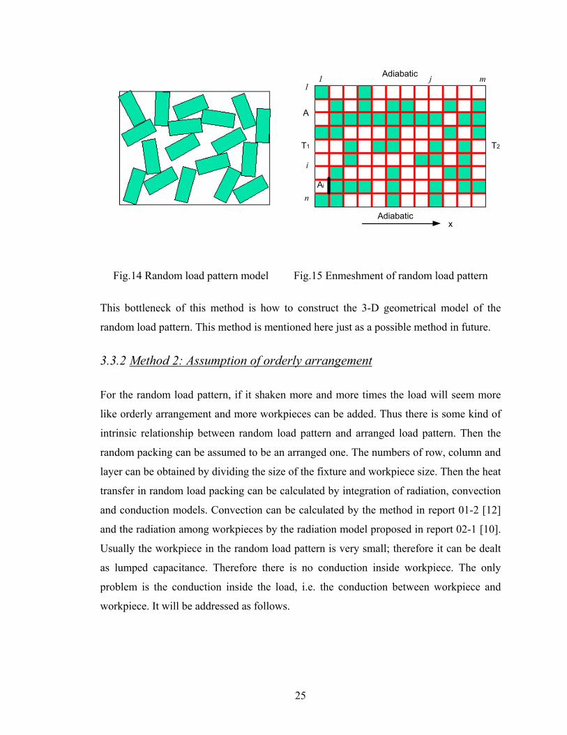
If a sample region of the three-dimensional model of random load pattern is constructed,
the effective thermal conductivity can be calculated by finite difference method. Suppose
the random load pattern model is constructed as Fig. 13, then enmesh the model, the
enmeshment is shown in Fig. 14. Suppose one pair of two opposite sides is adiabatic, the
other pair of the two opposite sides is suddenly exerted to different constant temperatures
T1 and T2. Then heat transfer inside the region will occur under the drive of temperature
gradient. The constant temperatures at two sides serve as boundary condition. In the finite
difference model there are two kinds of elements, part and air. Thus, the thermal
properties of all elements are known. Then the heat transfer between the two sides can be
calculated by equation (11) (For three-dimensional problem, two pairs of opposite sides
are assumed as adiabatic). As the heat transfer between the two sides reach static state,
the heat flow between the two sides can be calculated by equation (12).
∑∆
−+∑=
=
+
=
n
i
jijiijim
j xTTA
Q1
,,1
1
)(2
)( λλ (16)
where ∆x is the element size in X direction, Ai is the surface area of an element
perpendicular X direction, λi is the thermal conductivity of i element, m and n are the
numbers of elements in X and Y directions, respectively.
Then the effective thermal conductivity can be calculated by
LTTA
Qeff )( 12 −
=λ (17)
where A is the total side surface area.
When the thermal effective thermal conductivity is obtained, then it can be used back to
calculate the heat transfer in the same load pattern.
24
T2
Ai
A
xAdiabatic
T1
i
11 j
n
Adiabatic m
Fig.14 Random load pattern model Fig.15 Enmeshment of random load pattern
This bottleneck of this method is how to construct the 3-D geometrical model of the
random load pattern. This method is mentioned here just as a possible method in future.
3.3.2 Method 2: Assumption of orderly arrangement
For the random load pattern, if it shaken more and more times the load will seem more
like orderly arrangement and more workpieces can be added. Thus there is some kind of
intrinsic relationship between random load pattern and arranged load pattern. Then the
random packing can be assumed to be an arranged one. The numbers of row, column and
layer can be obtained by dividing the size of the fixture and workpiece size. Then the heat
transfer in random load packing can be calculated by integration of radiation, convection
and conduction models. Convection can be calculated by the method in report 01-2 [12]
and the radiation among workpieces by the radiation model proposed in report 02-1 [10].
Usually the workpiece in the random load pattern is very small; therefore it can be dealt
as lumped capacitance. Therefore there is no conduction inside workpiece. The only
problem is the conduction inside the load, i.e. the conduction between workpiece and
workpiece. It will be addressed as follows.
25
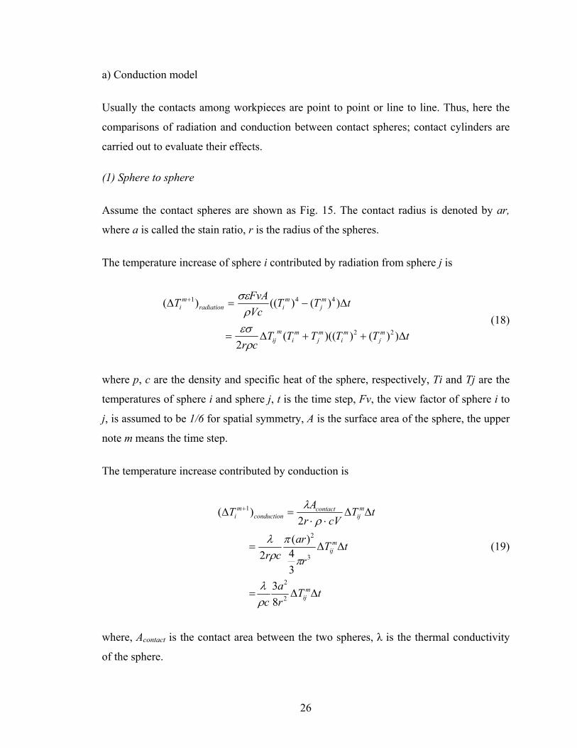
a) Conduction model
Usually the contacts among workpieces are point to point or line to line. Thus, here the
comparisons of radiation and conduction between contact spheres; contact cylinders are
carried out to evaluate their effects.
(1) Sphere to sphere
Assume the contact spheres are shown as Fig. 15. The contact radius is denoted by ar,
where a is called the stain ratio, r is the radius of the spheres.
The temperature increase of sphere i contributed by radiation from sphere j is
tTTTTTcr
tTTVcFvAT
mj
mi
mj
mi
mij
mj
miradiation
mi
∆++∆=
∆−=∆ +
))())(((2
))()(()(
22
441
ρεσρ
σε
(18)
where p, c are the density and specific heat of the sphere, respectively, Ti and Tj are the
temperatures of sphere i and sphere j, t is the time step, Fv, the view factor of sphere i to
j, is assumed to be 1/6 for spatial symmetry, A is the surface area of the sphere, the upper
note m means the time step.
The temperature increase contributed by conduction is
tTra
c
tTr
arcr
tTcVr
AT
mij
mij
mij
contactconduction
mi
∆∆=
∆∆=
∆∆⋅⋅
=∆ +
2
2
3
2
1
83
34
)(2
2)(
ρλ
π
πρ
λρ
λ
(19)
where, Acontact is the contact area between the two spheres, λ is the thermal conductivity
of the sphere.
26
Then the ratio of the temperature increase contribution by radiation to conduction is
2
22
1
1
3))())(((4
)()(
aTTTTr
TT m
jm
imj
mi
conductionm
i
radiationm
i
⋅
++=
∆∆
+
+
λεσ
(20)
For carbon steel, λ = 40W/m-K. The strain ratio a is very small because we assume there
is stiff contact. Assume Ti = 300K. The ratio vs. radiuses of the sphere, temperature of Tj
and strain ratio are plotted out in Fig. 16.
Ti
Tj
0 0.01 0.02 0.03 0.040
5
10
15
20
25
3030
0
4 σ⋅ ε⋅ T1 T2+( )⋅ T12 T22+( )⋅r
83⋅ λ⋅ a2⋅⋅
4 σ⋅ ε⋅ T3 T2+( )⋅ T32 T22+( ) r
83⋅ λ⋅ a2⋅⋅
4 σ⋅ ε⋅ T1 T2+( )⋅ T12 T22+( )⋅r
83⋅ λ⋅ a12⋅⋅
4 σ⋅ ε⋅ T1 T2+( )⋅ T32 T22+( )⋅r
83⋅ λ⋅ a12⋅⋅
4 σ⋅ ε⋅ T1 T2+( )⋅ T12 T22+( )⋅r
83⋅ λ⋅ a22⋅⋅
4 σ⋅ ε⋅ T1 T2+( )⋅ T32 T22+( )⋅r
83⋅ λ⋅ a22⋅⋅
0.050 rm
a=0.
01, T
j=12
00K
a=0.02, Tj=1200K
a=0.
005,
Tj=
1200
K
a=0.01, Tj=500K
a=0.02, Tj=500K
a=0.
005,
Tj=
500K
conductionm
i
radiationm
i
TT
)()(
1
1
+
+
∆∆
Fig. 16 Comparison of radiation and conduction between contact spheres
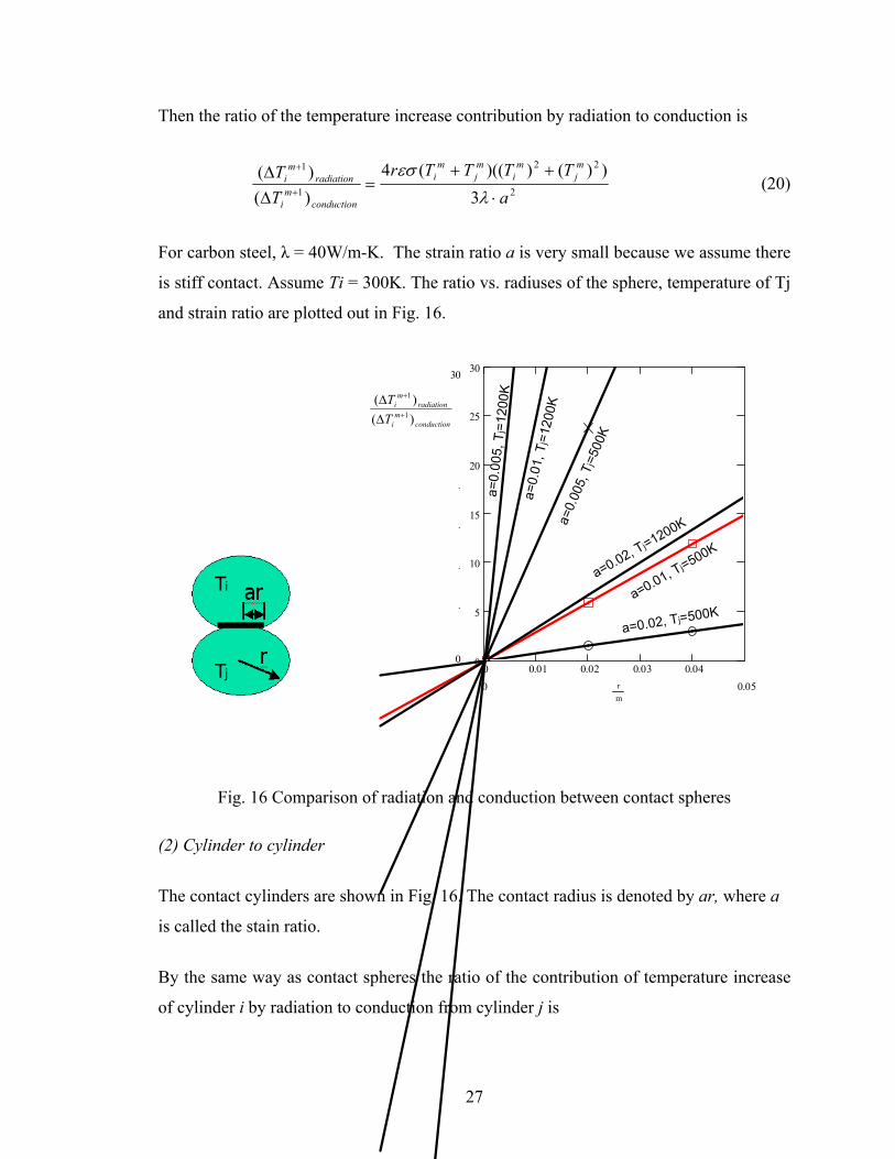
(2) Cylinder to cylinder
The contact cylinders are shown in Fig. 16. The contact radius is denoted by ar, where a
is called the stain ratio.
By the same way as contact spheres the ratio of the contribution of temperature increase
of cylinder i by radiation to conduction from cylinder j is
27
aTTTTr
TT m
jm
imj
mi
conductionm
i
radiationm
i
⋅
++=
∆∆
+
+
λεσ
3))())(((
)()( 22
1
1
(21)
For carbon steel, λ = 40W/m-K. Assume Ti = 300K. The ratio vs radius of the cylinder,
temperature Tj and strain ratio are plotted out in Fig. 17.
TjTi
arr
0 0.01 0.02 0.03 0.040
0.5
1
1.5
2
2.5
33
0
π ε⋅ σ⋅ T1 T2+( )⋅ T12 T22+( )⋅r
3 λ⋅ a⋅⋅
π ε σ⋅ T3 T2+( )⋅ T32 T22+( ) r
3 λ⋅ a⋅⋅
π ε σ⋅ T3 T2+( )⋅ T12 T22+( ) r
3 λ⋅ a1⋅⋅
π ε σ⋅ T3 T2+( )⋅ T32 T22+( ) r
3 λ⋅ a1⋅⋅
π ε σ⋅ T3 T2+( )⋅ T12 T22+( ) r
3 λ⋅ a2⋅⋅
π ε σ⋅ T3 T2+( )⋅ T32 T22+( ) r
3 λ⋅ a2⋅⋅
0.050 rm
conductionm
i
radiationm
i
TT
)()(
1
1
+
+
∆∆
a=0.02, Tj=500Ka=0.01, Tj=500K
a=0.0
05, T
j=500
K
a=0.
02, T
j=120
0K
a=0.
01, T
j=12
00K
a=0.
005,
Tj=
1200
K
Fig. 17 Comparison of radiation and conduction between cylinders
It can be seen from Fig. 16 and Fig. 17 that the radiation between sphere and sphere,
cylinder and cylinder is greater than the conduction between them. Therefore the
conduction inside the random load can be neglected. Actually the thermal conductivity
between contact spheres or cylinders is smaller than the solid phase because of contact
thermal resistance. So the ratio will be greater. As the radius r and temperature of Tj
increases, the ratio will increase. As the strain ratio a decreases the ratio increases.
As the radius of the sphere or cylinder is less than 1mm the conduction will take main
part. That agrees with the results for powder mentioned in the review section.
28

3.4 Conclusions
Random load pattern related studies are reviewed and analyzed. Two methods are
proposed to solve the heat transfer in random load pattern. One is based on the measured
results, from which the effective thermal conductivity can be calculated by reverse
method. The second one is to treat the random load pattern as orderly arrangement.
Radiation and convection are considered, while the conduction is neglected.
29

CHAPTER 4. CASE STUDIES OF RANDOM LOAD MODEL
In order to validate the random load model, case studies were conducted in two different
companies. The calculation results with the random load model were compared with
measured data in production.
4.1 Case Study 1 :(CASCO)
The first case study was carried out in Bodycote Thermal Processing plant, Worcester
Massachusetts. The workpieces, as seen in Fig. 18, shows that they are small in size and
also large in number.
4.1.1 Workpiece data
The workpieces used for the study are shown in Fig. 18 and Table 1.
Fig. 18 Casco workpieces
30
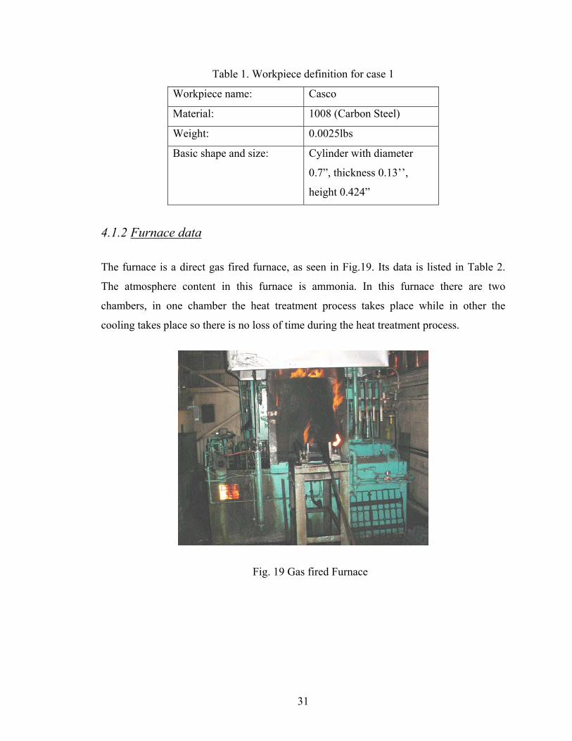
Table 1. Workpiece definition for case 1
Workpiece name: Casco
Material: 1008 (Carbon Steel)
Weight: 0.0025lbs
Basic shape and size: Cylinder with diameter
0.7”, thickness 0.13’’,
height 0.424”
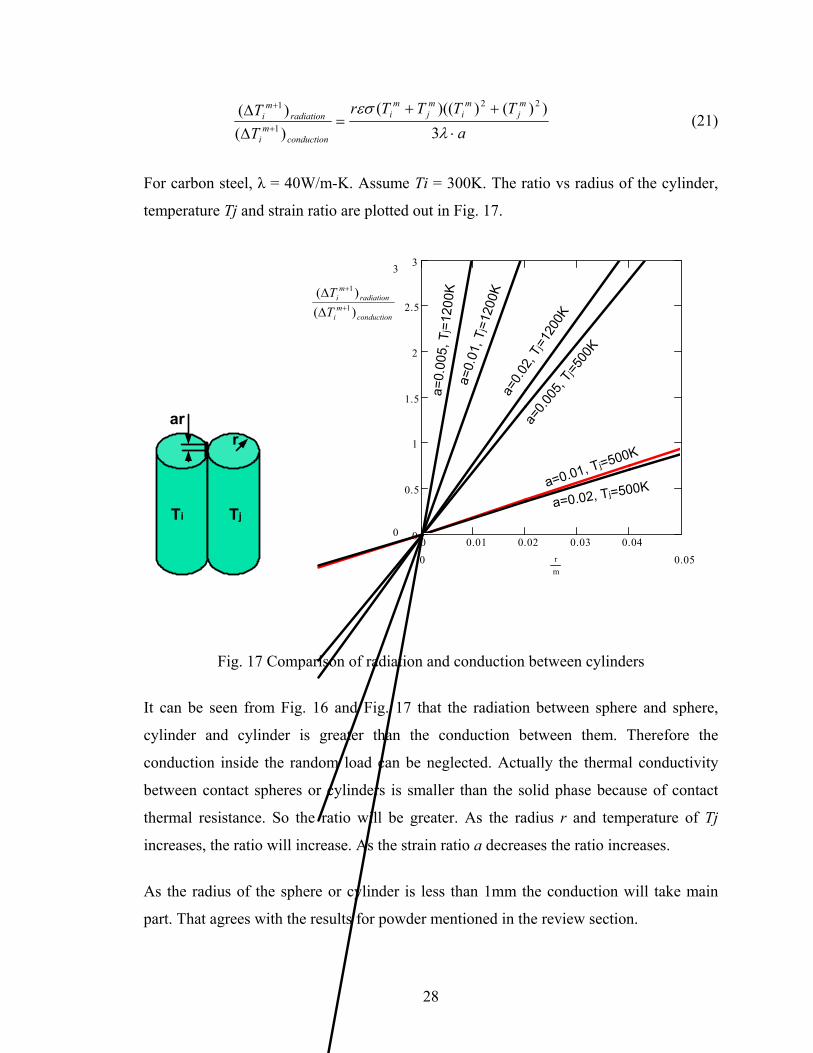
4.1.2 Furnace data
The furnace is a direct gas fired furnace, as seen in Fig.19. Its data is listed in Table 2.
The atmosphere content in this furnace is ammonia. In this furnace there are two
chambers, in one chamber the heat treatment process takes place while in other the
cooling takes place so there is no loss of time during the heat treatment process.
Fig. 19 Gas fired Furnace
31
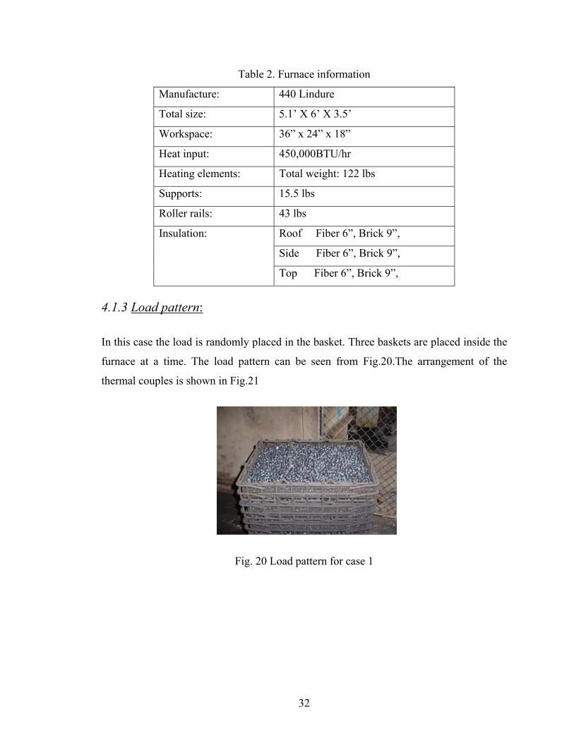
Table 2. Furnace information
Manufacture: 440 Lindure
Total size: 5.1’ X 6’ X 3.5’
Workspace: 36” x 24” x 18”
Heat input: 450,000BTU/hr
Heating elements: Total weight: 122 lbs
Supports: 15.5 lbs
Roller rails: 43 lbs
Roof Fiber 6”, Brick 9”,
Side Fiber 6”, Brick 9”,
Insulation:
Top Fiber 6”, Brick 9”,
4.1.3 Load pattern:
In this case the load is randomly placed in the basket. Three baskets are placed inside the
furnace at a time. The load pattern can be seen from Fig.20.The arrangement of the
thermal couples is shown in Fig.21
Fig. 20 Load pattern for case 1
32
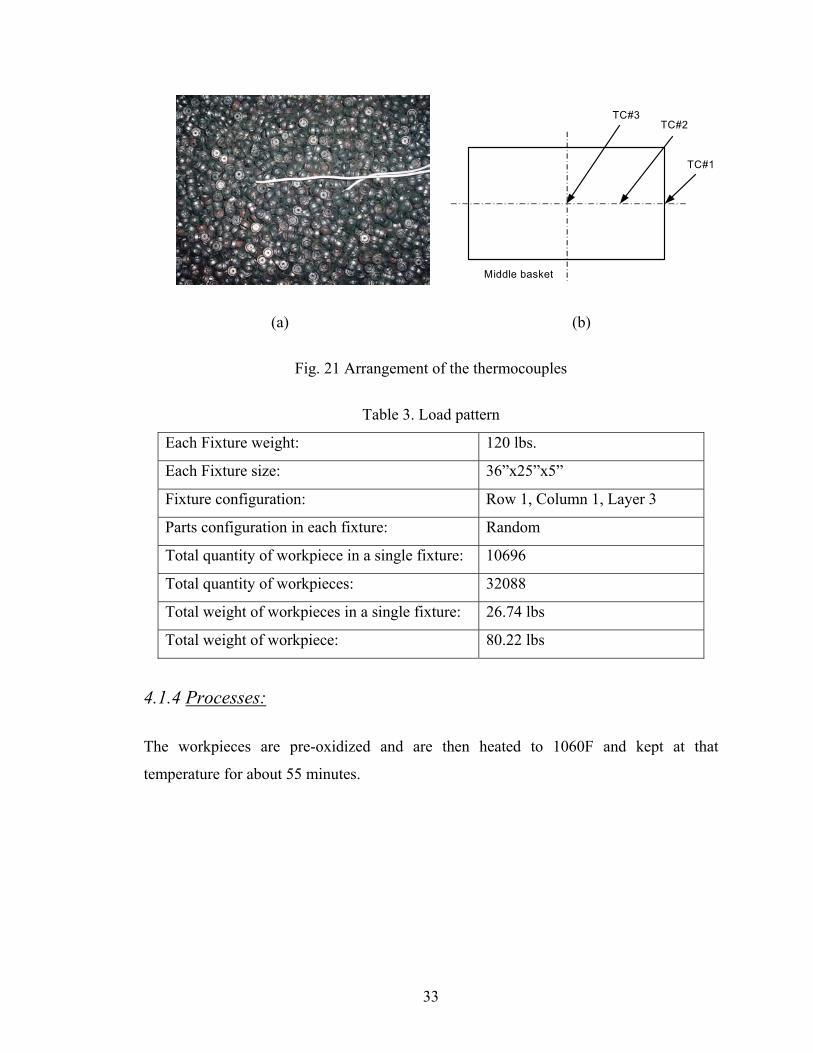
TC#1
TC#2TC#3
Middle basket
(a) (b)
Fig. 21 Arrangement of the thermocouples
Table 3. Load pattern
Each Fixture weight: 120 lbs.
Each Fixture size: 36”x25”x5”
Fixture configuration: Row 1, Column 1, Layer 3
Parts configuration in each fixture: Random
Total quantity of workpiece in a single fixture: 10696
Total quantity of workpieces: 32088
Total weight of workpieces in a single fixture: 26.74 lbs
Total weight of workpiece: 80.22 lbs
4.1.4 Processes:
The workpieces are pre-oxidized and are then heated to 1060F and kept at that
temperature for about 55 minutes.
33
4.1.5 Observation and Calculations:
0
200
400
600
800
1000
1200
0 20 40 60 80Time (min)
Tem
pera
ture
(F) Thermal Schedule
T_fce
T_fast (calculated)
T_slow (T_#3) (calculated)
T_#1(measured)
T_#3 (measured)
T_#1 (calculated)
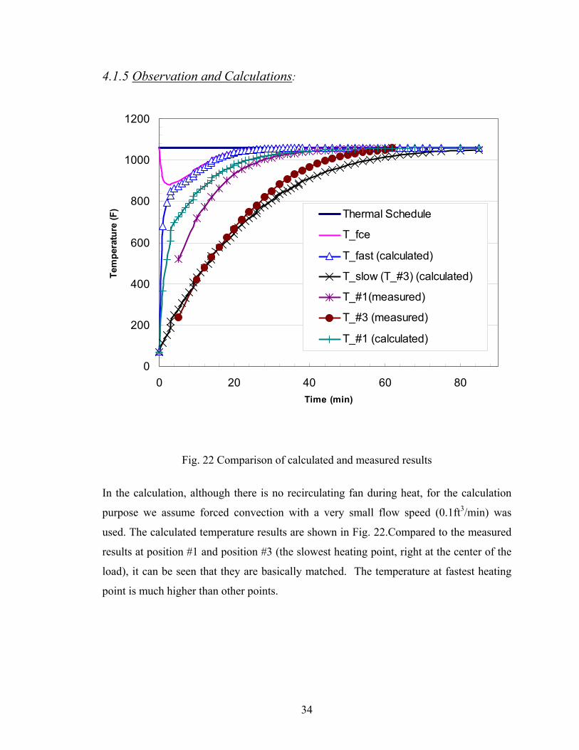
Fig. 22 Comparison of calculated and measured results
In the calculation, although there is no recirculating fan during heat, for the calculation
purpose we assume forced convection with a very small flow speed (0.1ft3/min) was
used. The calculated temperature results are shown in Fig. 22.Compared to the measured
results at position #1 and position #3 (the slowest heating point, right at the center of the
load), it can be seen that they are basically matched. The temperature at fastest heating
point is much higher than other points.
34
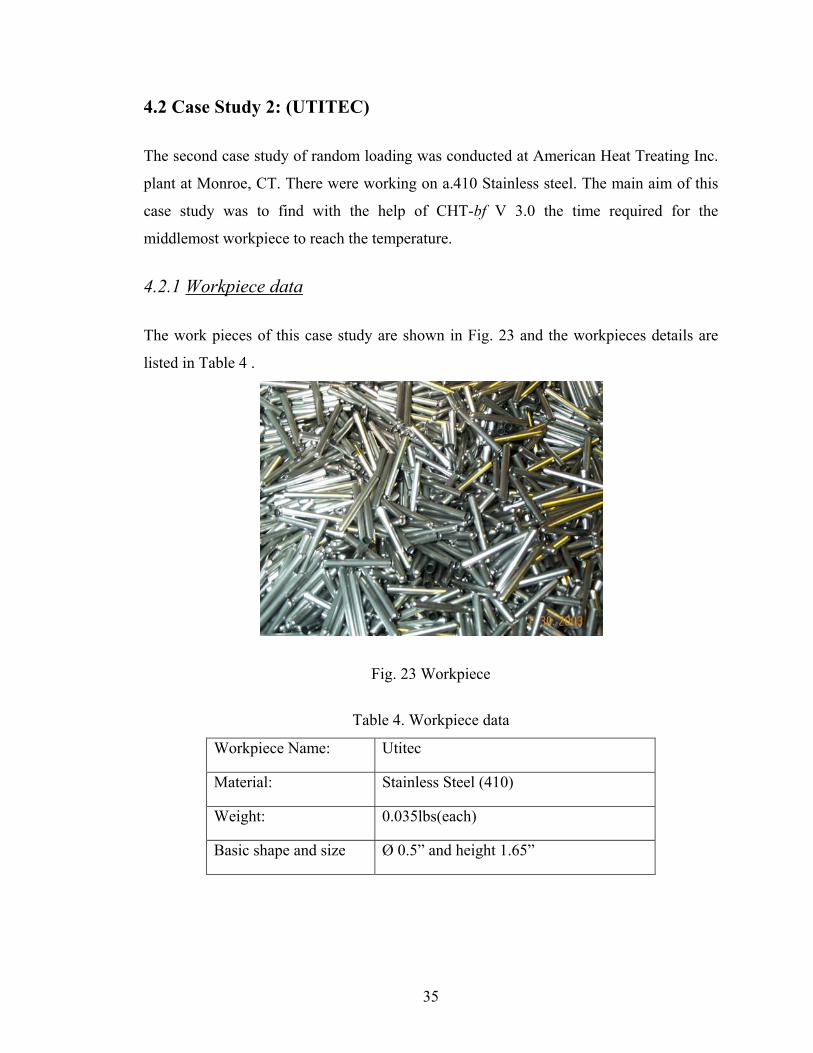
4.2 Case Study 2: (UTITEC)
The second case study of random loading was conducted at American Heat Treating Inc.
plant at Monroe, CT. There were working on a.410 Stainless steel. The main aim of this
case study was to find with the help of CHT-bf V 3.0 the time required for the
middlemost workpiece to reach the temperature.
4.2.1 Workpiece data
The work pieces of this case study are shown in Fig. 23 and the workpieces details are
listed in Table 4 .
Fig. 23 Workpiece
Table 4. Workpiece data
Workpiece Name: Utitec
Material: Stainless Steel (410)
Weight: 0.035lbs(each)
Basic shape and size Ø 0.5” and height 1.65”
35
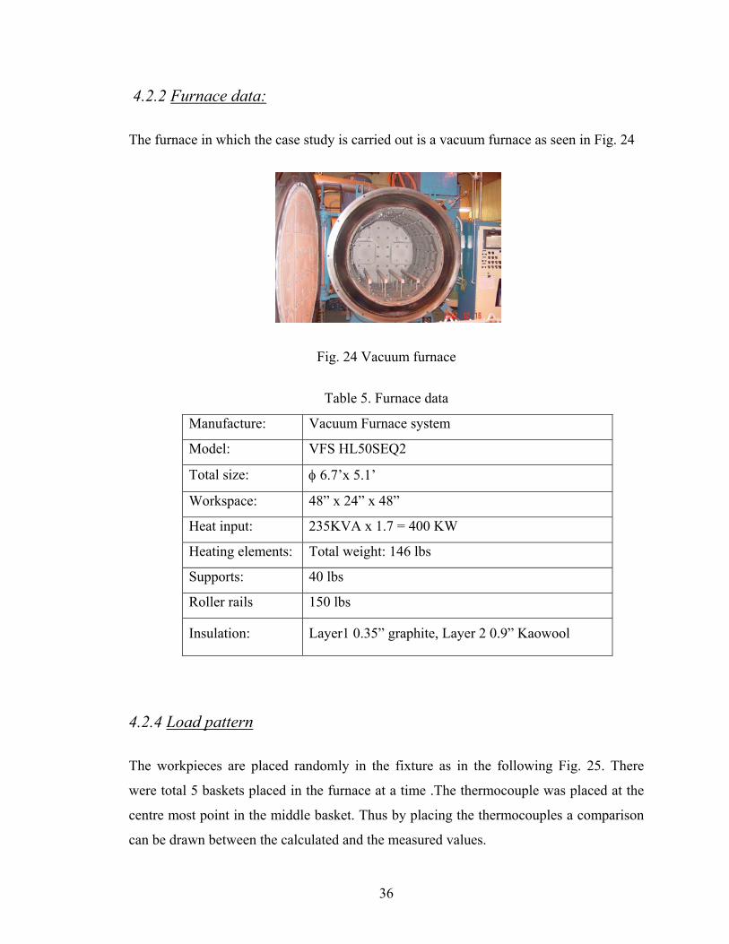
4.2.2 Furnace data:
The furnace in which the case study is carried out is a vacuum furnace as seen in Fig. 24
Fig. 24 Vacuum furnace
Table 5. Furnace data
Manufacture: Vacuum Furnace system
Model: VFS HL50SEQ2
Total size: φ 6.7’x 5.1’
Workspace: 48” x 24” x 48”
Heat input: 235KVA x 1.7 = 400 KW
Heating elements: Total weight: 146 lbs
Supports: 40 lbs
Roller rails 150 lbs
Insulation: Layer1 0.35” graphite, Layer 2 0.9” Kaowool
4.2.4 Load pattern
The workpieces are placed randomly in the fixture as in the following Fig. 25. There
were total 5 baskets placed in the furnace at a time .The thermocouple was placed at the
centre most point in the middle basket. Thus by placing the thermocouples a comparison
can be drawn between the calculated and the measured values.
36

Fig. 25 Load pattern and arrangement
Table 6. Load pattern
Fixture type (basket/plate) Basket
Fixture shape (round/rectangular) Rectangular
Side wall, bottom (solid, net-like) Net like
Each Fixture weight: 30 lbs
Each Fixture size: 23.5 ” x 14.5” x 6”
Fixture configuration: Random
Total quantity of workpiece in a single fixture: 8711
Total quantity of workpiece 43555
Total weight of workpiece in a single fixture: 304.5 lbs
37
4.2.5 Observation and Conclusion
Time Vs Temperature
0
200
400
600
800
1000
1200
1400
1600
0 20 40 60 80 100 120 140 160 180Time(mins)
Tem
pera
ture
(F)
set ptFurnace ptfastslowslowestmeasured slow
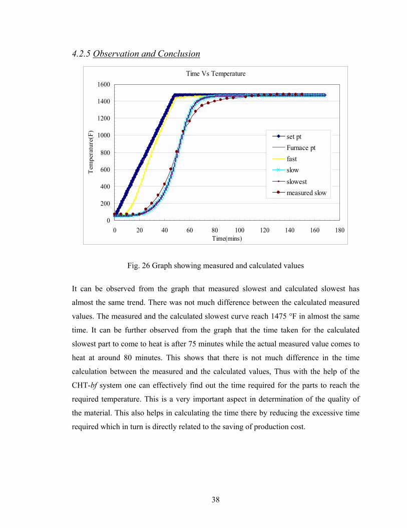
Fig. 26 Graph showing measured and calculated values
It can be observed from the graph that measured slowest and calculated slowest has
almost the same trend. There was not much difference between the calculated measured
values. The measured and the calculated slowest curve reach 1475 °F in almost the same
time. It can be further observed from the graph that the time taken for the calculated
slowest part to come to heat is after 75 minutes while the actual measured value comes to
heat at around 80 minutes. This shows that there is not much difference in the time
calculation between the measured and the calculated values, Thus with the help of the
CHT-bf system one can effectively find out the time required for the parts to reach the
required temperature. This is a very important aspect in determination of the quality of
the material. This also helps in calculating the time there by reducing the excessive time
required which in turn is directly related to the saving of production cost.
38

4.3 Conclusion
The case studies will help to validate a relationship between the measured and the
calculated values. From the results, it can be seen that the prediction results are very close
to the measured data. The first case study was done to check the efficiency of the system
while the second case study was done to for the prediction of the load temperature. Thus
the system is validated and then used for the predicting the temperature.
39

CHAPTER 5. CONTINOUS FURNACE MODELING 5.1 Background of Heat Treatment in Continuous Furnaces
Continuous furnaces are widely used for the heat treatment of mass production parts. So
to optimize the heat treating process in continuous furnace is of great significance.
A tool for part load design and temperature control in batch furnaces has been developed
and put into application under the fund of Center for Heat Treating Excellence. During
the former two projects funded by CHTE: 1) Development Of An Analytical Tool For
Part Load Design And Temperature Control Within Loaded Furnace And Parts [9-13]
and 2) Enhancement Of Computerized Heat Treating Process Planning System
(CAHTPS) [14,15], we have visited many member companies of CHTE and investigated
the applications of heat treating technology in the United States. In the investigation we
also acquired a lot of information on continuous furnaces, which be seen in the former
report [1]. Meanwhile the mathematical models for batch furnace are also helpful for the
development of module for heat treating processes in continuous furnace. The aim of the
development is to achieve a tool for the optimization of load pattern and furnace control
including movement and temperature distribution.
5.2 Classification of Continuous Furnaces
Continuous furnaces basically consist of pusher and conveyor furnaces.
1) Pusher furnaces
Pusher furnaces include Skid-Rail furnace and Roller rails furnace. A pusher furnace uses
the “tray-on-tray” concept to move workpiece through the furnace. The pusher
mechanism pushes a solid row of trays from the charge end until a tray is properly
located and proven in position at the discharge end for removal. On a timed basis, the
trays are successively moved through the furnace. The cycle time through the furnace is
varied only by changing the push intervals. Fig. 27 shows a typical rotary-retort heat
treating furnace for continuous carburizing. Because the front end of the furnace must be
open to allow continuous charging, sufficient carburizing gas must be fed into the furnace
40
to prevent the admission of outside air. Fig. 28 shows a schematic view of tray movement
in a pusher furnace.
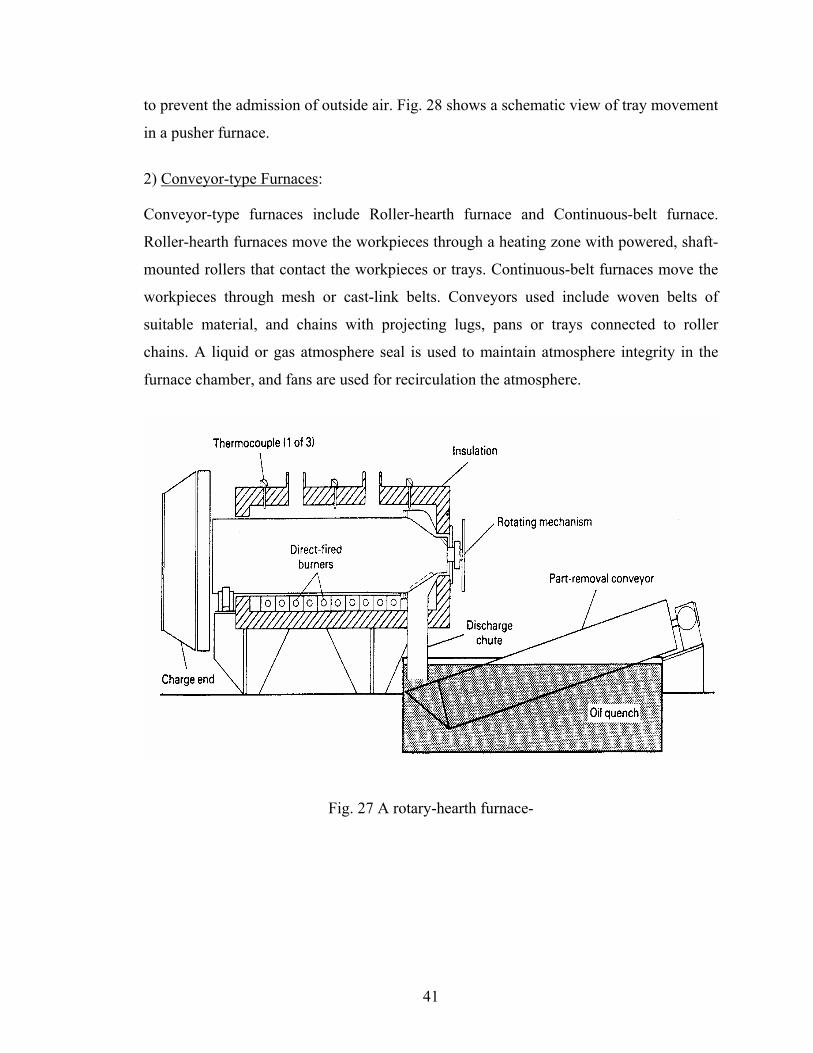
2) Conveyor-type Furnaces:
Conveyor-type furnaces include Roller-hearth furnace and Continuous-belt furnace.
Roller-hearth furnaces move the workpieces through a heating zone with powered, shaft-
mounted rollers that contact the workpieces or trays. Continuous-belt furnaces move the
workpieces through mesh or cast-link belts. Conveyors used include woven belts of
suitable material, and chains with projecting lugs, pans or trays connected to roller
chains. A liquid or gas atmosphere seal is used to maintain atmosphere integrity in the
furnace chamber, and fans are used for recirculation the atmosphere.
Fig. 27 A rotary-hearth furnace-
41

Fig. 28 A schematic view of tray movement in a pusher furnace
5.3 Studies about Continuous Furnaces
There are few software about the optimization of heat treating process in continuous
furnace. Among them FurnXpert program is developed to optimize furnace design and
operation [16]. It can be used for any type of batch and continuous furnaces. An example
for continuous belt furnace for sintering process in powder metallurgy was given. The
program mainly focuses on the heat balance of the furnace. The load pattern is just
aligned load pattern with just one layer and it cannot deal with the condition of
workpieces loaded in the fixtures. While, in this condition the workpieces inside the
fixture are heated by adjacent workpieces, not directly by furnace. Fig. 29 shows an
interface of load pattern specifications in FurnXpert. The result curves are shown in Fig.
30. In the program it mentioned that finite element method is used for the heat transfer
inside the part. However, nothing details about finite element method was presented.
Other software such as ICON and DCON [17] are developed in the mid 1990’s. They are
just for very simple workpiece shape and based on DOS, so they are not proper for the
optimization of heat treating process of arbitrary shape workpieces.
42

Fig. 29 The load pattern for continuous belt in FurnXpert software [16]
Fig. 30 The result illustration of FurnXpert software [16]
43
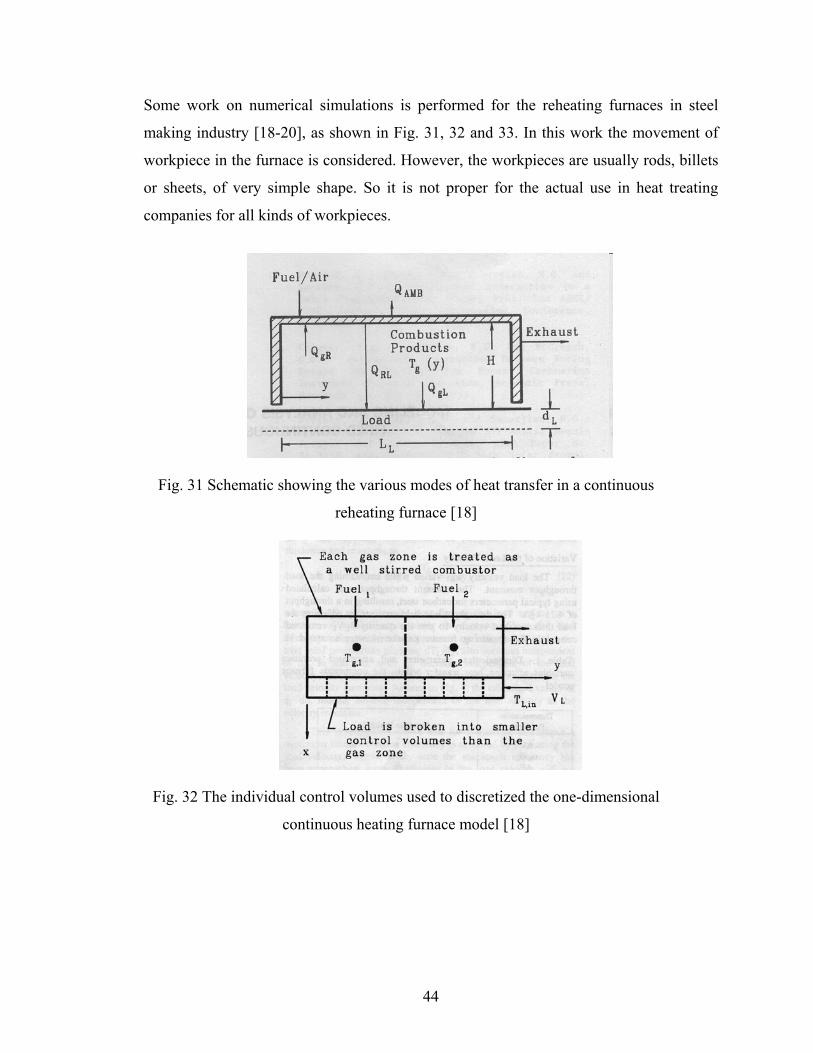
Some work on numerical simulations is performed for the reheating furnaces in steel
making industry [18-20], as shown in Fig. 31, 32 and 33. In this work the movement of
workpiece in the furnace is considered. However, the workpieces are usually rods, billets
or sheets, of very simple shape. So it is not proper for the actual use in heat treating
companies for all kinds of workpieces.
Fig. 31 Schematic showing the various modes of heat transfer in a continuous
reheating furnace [18]
Fig. 32 The individual control volumes used to discretized the one-dimensional
continuous heating furnace model [18]
44
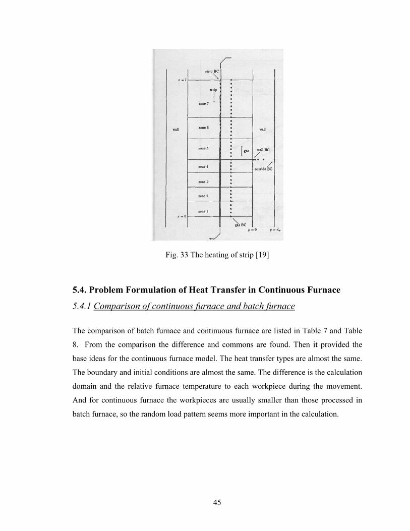
Fig. 33 The heating of strip [19]
5.4. Problem Formulation of Heat Transfer in Continuous Furnace
5.4.1 Comparison of continuous furnace and batch furnace
The comparison of batch furnace and continuous furnace are listed in Table 7 and Table
8. From the comparison the difference and commons are found. Then it provided the
base ideas for the continuous furnace model. The heat transfer types are almost the same.
The boundary and initial conditions are almost the same. The difference is the calculation
domain and the relative furnace temperature to each workpiece during the movement.
And for continuous furnace the workpieces are usually smaller than those processed in
batch furnace, so the random load pattern seems more important in the calculation.
45
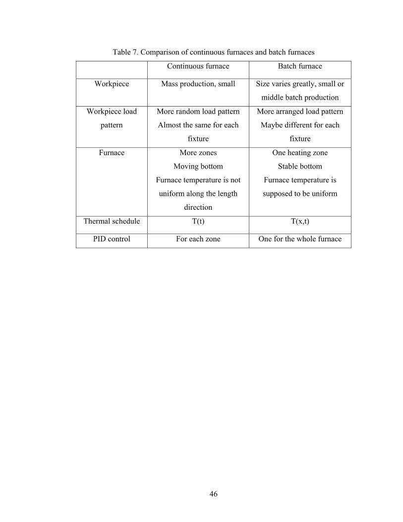
Table 7. Comparison of continuous furnaces and batch furnaces
Continuous furnace Batch furnace
Workpiece Mass production, small Size varies greatly, small or
middle batch production
Workpiece load
pattern
More random load pattern
Almost the same for each
fixture
More arranged load pattern
Maybe different for each
fixture
Furnace More zones
Moving bottom
Furnace temperature is not
uniform along the length
direction
One heating zone
Stable bottom
Furnace temperature is
supposed to be uniform
Thermal schedule T(t) T(x,t)
PID control For each zone One for the whole furnace
46
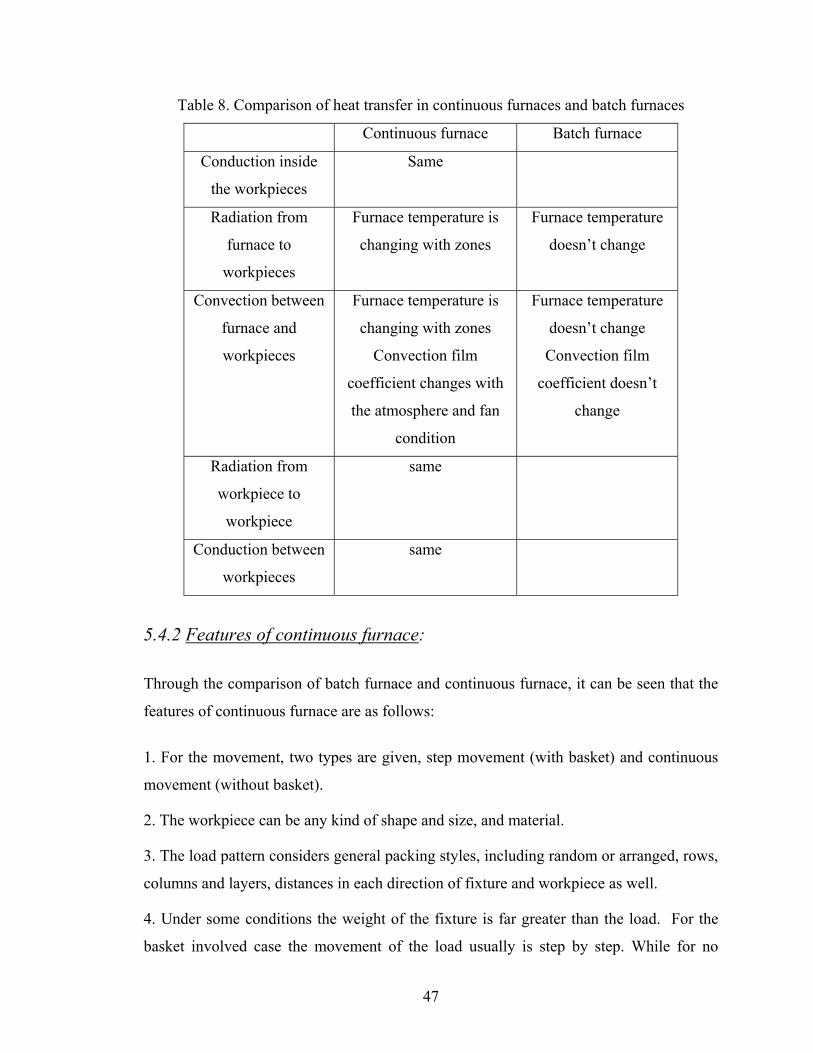
Table 8. Comparison of heat transfer in continuous furnaces and batch furnaces
Continuous furnace Batch furnace
Conduction inside
the workpieces
Same
Radiation from
furnace to
workpieces
Furnace temperature is
changing with zones
Furnace temperature
doesn’t change
Convection between
furnace and
workpieces
Furnace temperature is
changing with zones
Convection film
coefficient changes with
the atmosphere and fan
condition
Furnace temperature
doesn’t change
Convection film
coefficient doesn’t
change
Radiation from
workpiece to
workpiece
same
Conduction between
workpieces
same
5.4.2 Features of continuous furnace:
Through the comparison of batch furnace and continuous furnace, it can be seen that the
features of continuous furnace are as follows:
1. For the movement, two types are given, step movement (with basket) and continuous
movement (without basket).
2. The workpiece can be any kind of shape and size, and material.
3. The load pattern considers general packing styles, including random or arranged, rows,
columns and layers, distances in each direction of fixture and workpiece as well.
4. Under some conditions the weight of the fixture is far greater than the load. For the
basket involved case the movement of the load usually is step by step. While for no
47
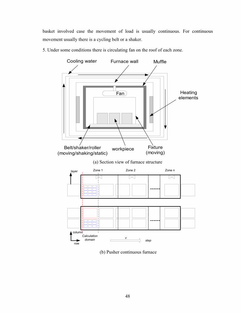
basket involved case the movement of load is usually continuous. For continuous
movement usually there is a cycling belt or a shaker.
5. Under some conditions there is circulating fan on the roof of each zone.
Cooling water Furnace wall
Belt/shaker/roller(moving/shaking/static)
workpiece Fixture(moving)
Muffle
Fan Heatingelements
(a) Section view of furnace structure
Zone 1 Zone 2 Zone n
vstep
Calculationdomain
row
column
layer
(b) Pusher continuous furnace
48
Zone 1 Zone 2 Zone n
vcontinuous
Calculationdomain
row
column
layer
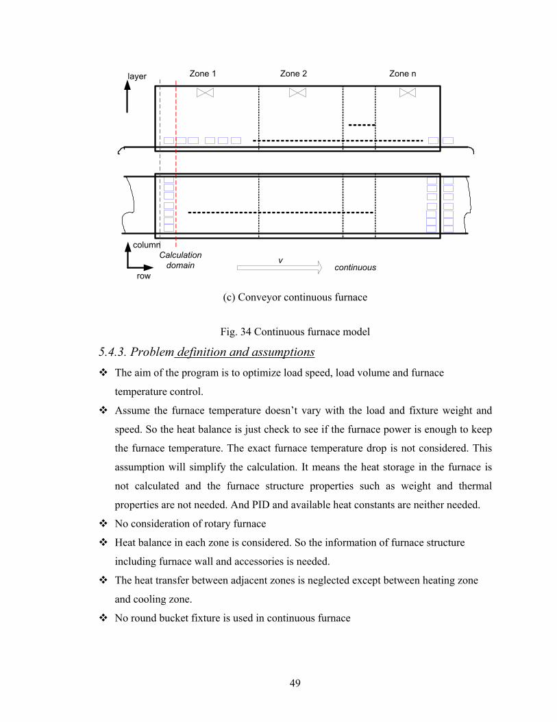
(c) Conveyor continuous furnace
Fig. 34 Continuous furnace model
5.4.3. Problem definition and assumptions The aim of the program is to optimize load speed, load volume and furnace
temperature control.
Assume the furnace temperature doesn’t vary with the load and fixture weight and
speed. So the heat balance is just check to see if the furnace power is enough to keep
the furnace temperature. The exact furnace temperature drop is not considered. This
assumption will simplify the calculation. It means the heat storage in the furnace is
not calculated and the furnace structure properties such as weight and thermal
properties are not needed. And PID and available heat constants are neither needed.
No consideration of rotary furnace
Heat balance in each zone is considered. So the information of furnace structure
including furnace wall and accessories is needed.
The heat transfer between adjacent zones is neglected except between heating zone
and cooling zone.
No round bucket fixture is used in continuous furnace
49
There can be no fixture. Fixture is defined here as that directly holds or support
workpieces and moves forward with workpieces. Fixture doesn’t include belt or
conveyor. The recycling belt or conveyors are also considered in the heat balance
calculation. They always have the same temperature as the fastest heated workpieces.
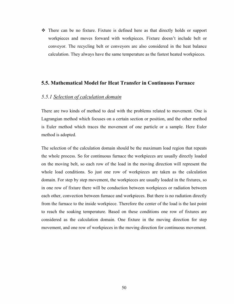
5.5. Mathematical Model for Heat Transfer in Continuous Furnace
5.5.1 Selection of calculation domain
There are two kinds of method to deal with the problems related to movement. One is
Lagrangian method which focuses on a certain section or position, and the other method
is Euler method which traces the movement of one particle or a sample. Here Euler
method is adopted.
The selection of the calculation domain should be the maximum load region that repeats
the whole process. So for continuous furnace the workpieces are usually directly loaded
on the moving belt, so each row of the load in the moving direction will represent the
whole load conditions. So just one row of workpieces are taken as the calculation
domain. For step by step movement, the workpieces are usually loaded in the fixtures, so
in one row of fixture there will be conduction between workpieces or radiation between
each other, convection between furnace and workpieces. But there is no radiation directly
from the furnace to the inside workpiece. Therefore the center of the load is the last point
to reach the soaking temperature. Based on these conditions one row of fixtures are
considered as the calculation domain. One fixture in the moving direction for step
movement, and one row of workpieces in the moving direction for continuous movement.
50
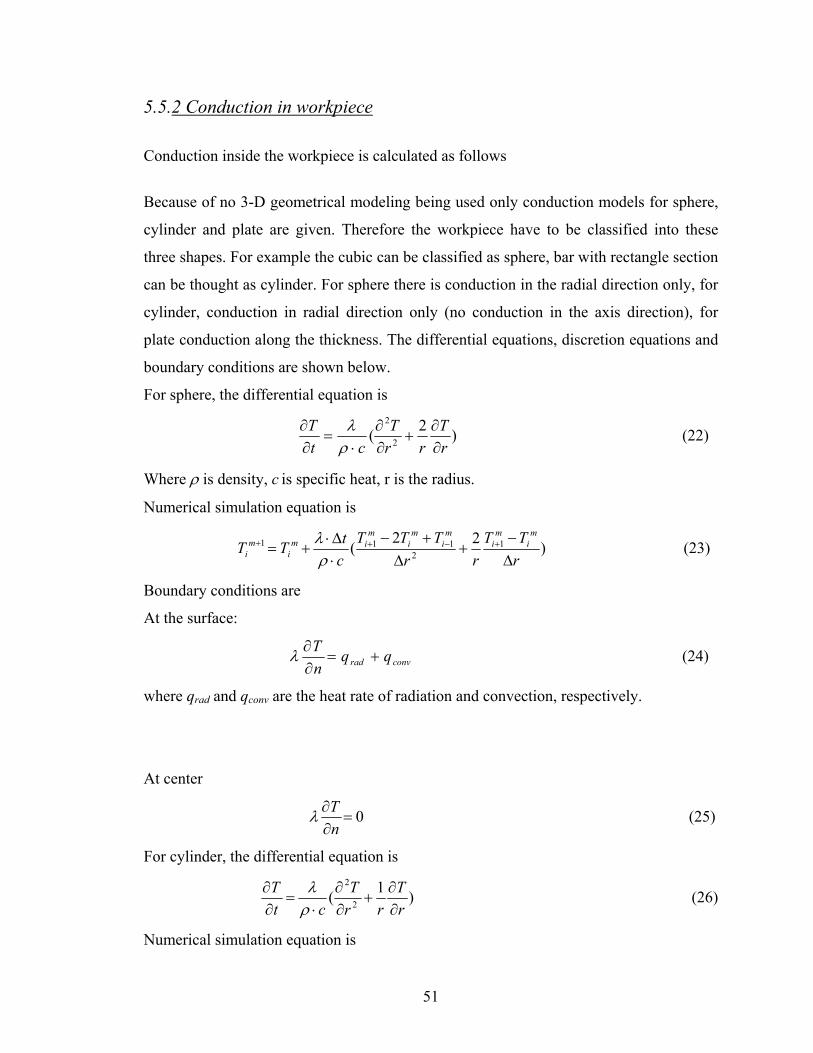
5.5.2 Conduction in workpiece
Conduction inside the workpiece is calculated as follows
Because of no 3-D geometrical modeling being used only conduction models for sphere,
cylinder and plate are given. Therefore the workpiece have to be classified into these
three shapes. For example the cubic can be classified as sphere, bar with rectangle section
can be thought as cylinder. For sphere there is conduction in the radial direction only, for
cylinder, conduction in radial direction only (no conduction in the axis direction), for
plate conduction along the thickness. The differential equations, discretion equations and
boundary conditions are shown below.
For sphere, the differential equation is
)2( 2
2
rT
rrT
ctT
∂∂
+∂∂
⋅=
∂∂
ρλ (22)
Where ρ is density, c is specific heat, r is the radius.
Numerical simulation equation is
)22( 12
111
rTT
rrTTT
ctTT
mi
mi
mi
mi
mim
im
i ∆−
+∆
+−⋅∆⋅
+= +−++
ρλ (23)
Boundary conditions are
At the surface:
convrad qqnT
+=∂∂λ (24)
where qrad and qconv are the heat rate of radiation and convection, respectively.
At center
0=∂∂
nTλ (25)
For cylinder, the differential equation is
)1( 2
2
rT
rrT
ctT
∂∂
+∂∂
⋅=
∂∂
ρλ (26)
Numerical simulation equation is
51
)12( 12
111
rTT
rrTTT
ctTT
mi
mi
mi
mi
mim
im
i ∆−
+∆
+−⋅∆⋅
+= +−++
ρλ (27)
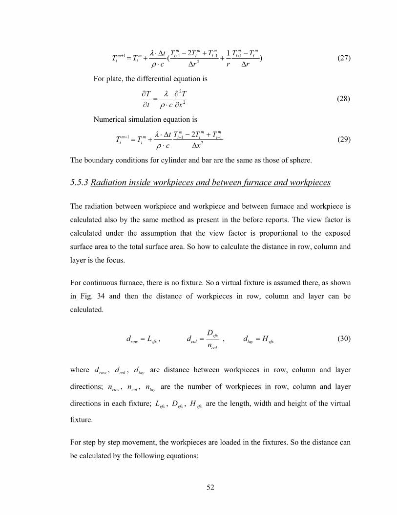
For plate, the differential equation is
2
2
xT
ctT
∂∂
⋅=
∂∂
ρλ (28)
Numerical simulation equation is
2111 2
xTTT
ctTT
mi
mi
mim
im
i ∆+−
⋅∆⋅
+= −++
ρλ (29)
The boundary conditions for cylinder and bar are the same as those of sphere.
5.5.3 Radiation inside workpieces and between furnace and workpieces
The radiation between workpiece and workpiece and between furnace and workpiece is
calculated also by the same method as present in the before reports. The view factor is
calculated under the assumption that the view factor is proportional to the exposed
surface area to the total surface area. So how to calculate the distance in row, column and
layer is the focus.
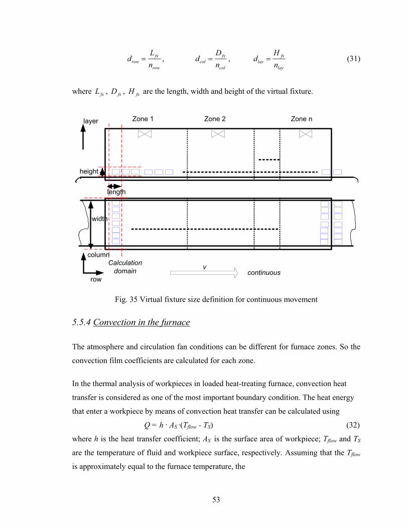
For continuous furnace, there is no fixture. So a virtual fixture is assumed there, as shown
in Fig. 34 and then the distance of workpieces in row, column and layer can be
calculated.
vfxrow Ld = , col
vfxcol n
Dd = , vfxlay Hd = (30)
where , , are distance between workpieces in row, column and layer
directions; , , are the number of workpieces in row, column and layer
directions in each fixture; , , are the length, width and height of the virtual
fixture.
rowd cold
row
layd
coln n layn
Lvfx vfxD vfxH
For step by step movement, the workpieces are loaded in the fixtures. So the distance can
be calculated by the following equations:
52
row
fxrow n
Ld = ,
col
fxcol n
Dd = ,
lay
fxlay n
Hd = (31)
where , , are the length, width and height of the virtual fixture. fxL fxD fxH
Zone 1 Zone 2 Zone n
vcontinuous
Calculationdomain
row
column
layer
height
length
width
Fig. 35 Virtual fixture size definition for continuous movement
5.5.4 Convection in the furnace
The atmosphere and circulation fan conditions can be different for furnace zones. So the
convection film coefficients are calculated for each zone.
In the thermal analysis of workpieces in loaded heat-treating furnace, convection heat
transfer is considered as one of the most important boundary condition. The heat energy
that enter a workpiece by means of convection heat transfer can be calculated using
Q = h · AS ·(Tflow - TS) (32)
where h is the heat transfer coefficient; AS is the surface area of workpiece; Tflow and TS
are the temperature of fluid and workpiece surface, respectively. Assuming that the Tflow
is approximately equal to the furnace temperature, the
53
calculation objective of h will be discussed in this appendix. The average convection
heat transfer coefficient, h, is generally calculated by[9]
** LNuLkh ⋅= (33)
where k is the thermal conductivity of gas (in W/m⋅K); L* is the equivalent length of part
related to the part geometry and size; and is the Nusselt number, *LNu
NuL* = f (Ra, Pr, Geometric shape, boundary conditions).
In the calculation the natural and forced convection are considered. And the aligned and
staggered load arrangements are also included in the convection film coefficients
calculation.
5.6 Numerical Calculations:
Based on the heat transfer principle, the following numerical calculation can be
formulated for the temperature estimation during the heat treating processes.
5.6.1 Furnace temperature distribution
Take the workpiece as a reference, the furnace temperature involved in the calculation
changes with the workpiece row number and time, it can be denoted as follows:
The furnace temperature distribution is the function of temperature zone and transition
zone. It is depicted as follows:
−∑<<+∑
+∑≤≤−∑−∑−+
−+
=
=
−
=
+===+
+
j
j
iij
j
iizonej
j
j
iij
j
iij
j
ii
jj
zonejjzonezonej
fce
LLdLLT
LLdLLLLdLL
TTT
dT
0
1
0_
10001
_)1(__
_
))(()( (34)
where i and j are the zone numbers, d is the distance from the beginning of the furnace, in
the range of 0 to the whole length of the furnace; L is the length of furnace zone.
54
5.6.2 Thermal schedule
The thermal schedule is the target thermal history of workpiece. The thermal schedule for
continuous furnace is different from that in batch furnace. In batch furnace the thermal
schedule is set before operation as ramp, preheats and soaks. It will not change during
heat treating process. But the thermal schedule for continuous furnace varies with the
movement speed of the workpieces. If the workpieces moves faster, i.e., the workpieces
will stay shorter in each zone, so the total time will become shorter. Finally, the cycle
will be shorter. If the movement speed slows down the workpieces will stay longer and
the cycle time become longer. Therefore the thermal schedule is determined by the
furnace zone temperature and the movement. Equation (34) shows the furnace zone
temperatures. By transformation of distance to time by the movement the thermal
schedule will be obtained.
The movement is classified into continuous and step by step, thus the transformation of
distance to time is also different for these two types of movements. The time for the
workpiece to move the distance d for continuous movement is
conVdt = (35)
where Vcon is the moving speed of continuous furnace.
Combine the above equation (34) and (35) and then the thermal schedule for continuous
movement can be obtained as follows.
−∑<<
+∑
+∑≤≤
−∑⋅
+
−+
=
=
−
=
+==
+
+
con
j
j
ii
con
j
j
ii
zonej
con
j
j
ii
con
j
j
ii
conjj
zonejjzonezonej
fce
V
LLt
V
LLT
V
LLt
V
LLtV
LLTT
TtT
0
1
0_
100
1
_)1(__
_
)()( (36)
The equation for step by step movement is
55
)(step
fxbreak
fx VL
tLdt +∆= (37)
where is the length of the fixture, fxL breakt∆ is the break time, V is the instant pushing
speed.
step
Combining equation (34) and (37), the thermal schedule for step by step movement is as
follows.
+∆
−<<
+∆
+
+∆
+≤≤
+∆
−⋅
+∆+
−+
=∑∑
∑∑
=
−
=
+==
+
+
step
fxbreak
fx
j
j
ii
step
fxbreak
fx
j
j
ii
zonej
step
fxbreak
fx
j
j
ii
step
fxbreak
fx
j
j
ii
step
fxbreak
fx
jj
zonejjzonezonej
fce
VL
t
L
LLt
VL
t
L
LLT
VL
t
L
LLt
VL
t
L
LLt
VL
t
LLL
TTT
tT
0
1
0_
100
1
_)1(__
_
)(
)( (38)
Usually it is very fast to push one tray inside the furnace, so the time for pushing can be
neglected. Then equation (38) and (39) will be as follows, respectively.
breakfx
tLdt ∆= (39)
∆
−∑<<
∆
+∑
∆
+∑≤≤
∆
−∑⋅
∆+
−+
=
=
−
=
+==
+
+
break
fx
j
j
ii
break
fx
j
j
ii
zonej
break
fx
j
j
ii
break
fx
j
j
ii
break
fx
jj
zonejjzonezonej
fce
tL
LLt
tL
LLT
tL
LLt
tL
LLt
tL
LLTT
T
tT
0
1
0_
100
1
_)1(__
_
)(
)( (40)
From equation (34), (36), (38) and (40) it can be seen that the furnace temperature is not
only the function of furnace length, but also the function of time, i.e., the workpiece is
56

fixed and the furnace is moving. The relative movement between furnace and workpiece
make the thermal schedule.
For continuous movement the thermal schedule is the same kind of shape as the furnace
temperature distribution, just with the distance axis changed to time axis. But for step by
step movement the workpieces are load in fixture. Thus, the temperature change of the
workpiece located at the fixture center is taken to represent the thermal schedule of the
calculation domain. The transformation of temperature-distance curve to temperature –
time curve for step by step movement is shown in Fig. 36 calculated by equation (38) or
(40).
Temp.
Zone1
TroomFixture
Breaktime
t1 t2 t3
T1
T2
Temp-time Temp-distance
Zone2 Zone3
TimeDistance or
Fig. 36 Relationship between temperature-time curve and temperature-distance curve
for step by step movement
57
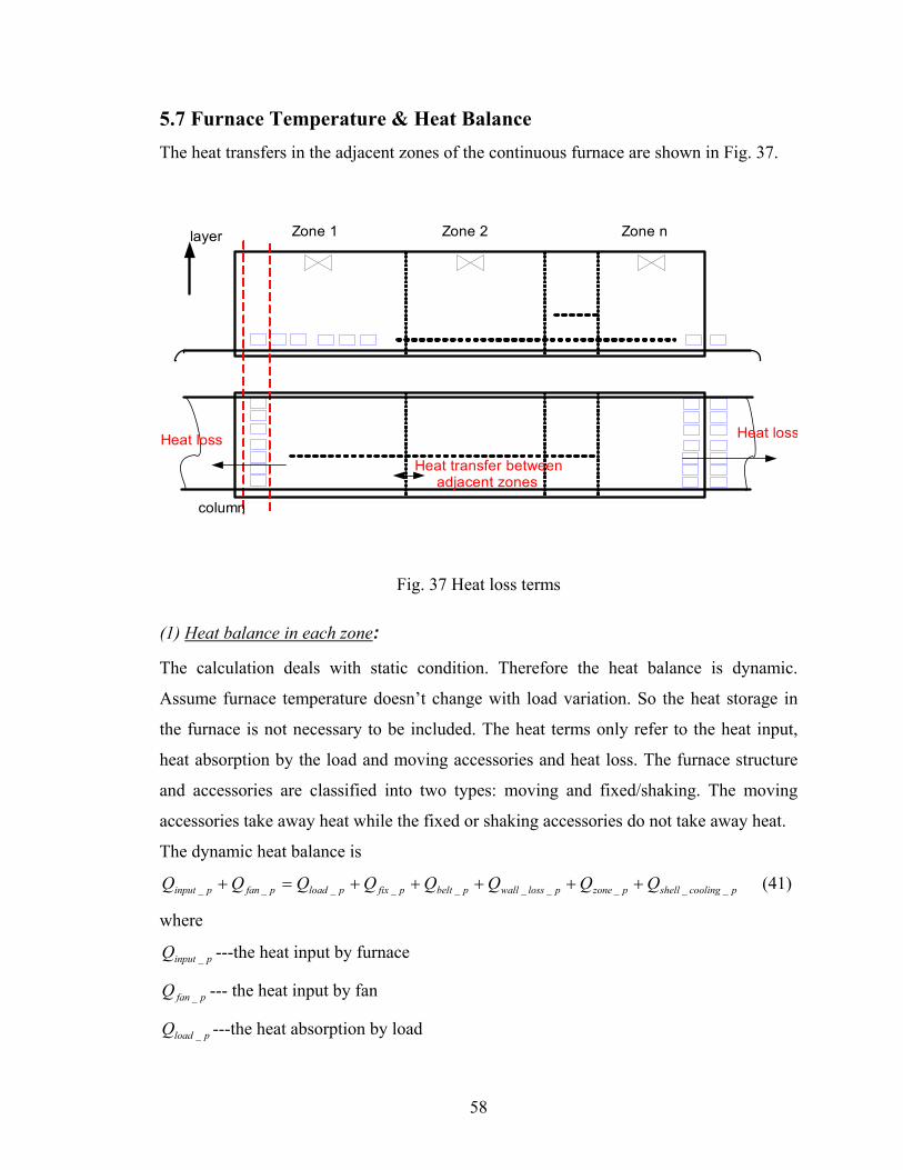
5.7 Furnace Temperature & Heat Balance The heat transfers in the adjacent zones of the continuous furnace are shown in Fig. 37.
Zone 1 Zone 2 Zone n
column
layer
Heat transfer betweenadjacent zones
Heat lossHeat loss
Fig. 37 Heat loss terms
(1) Heat balance in each zone:
The calculation deals with static condition. Therefore the heat balance is dynamic.
Assume furnace temperature doesn’t change with load variation. So the heat storage in
the furnace is not necessary to be included. The heat terms only refer to the heat input,
heat absorption by the load and moving accessories and heat loss. The furnace structure
and accessories are classified into two types: moving and fixed/shaking. The moving
accessories take away heat while the fixed or shaking accessories do not take away heat.
The dynamic heat balance is
pcoolingshellpzoneplosswallpbeltpfixploadpfanpinput QQQQQQQQ __________ +++++=+ (41)
where
pinputQ _ ---the heat input by furnace
pfanQ _ --- the heat input by fan
ploadQ _ ---the heat absorption by load
58

pfixQ _ ---the heat absorption by fixture
pbeltQ _ ---the heat absorption by belt
plosswallQ __ ---the heat loss from furnace wall
pzoneQ _ ---the heat transfer between zones and heat loss from the end zones
pcoolingshellQ __ ---the heat absorption by shell cooling water
From the above equation the heat input by furnace can be calculated indirectly as follows
pfanpcoolingshellpzoneplosswallpbeltpfixploadpinput QQQQQQQQ __________ −+++++= (42)
It is compared with the power of the furnace to see if it exceeds the power, which means
the heat balance cannot be kept. So the furnace temperature control system such as PID is
not considered.
The heat balance is calculated when a cycle is finished. Then the heat absorption in each
zone is calculated based on the relationship between calculation domain and zone length.
The procedure is initial furnace temperature- load temperature and all heat terms judge if
the heat balance can be kept. If it cannot be kept the calculation will give warning and
stop calculation, otherwise the calculation continues with the furnace temperature not
changed.
These heat terms are the functions of furnace temperature. Adjust the furnace temperature
to keep the heat balance. The heat input should also be calculated directly by the
connected heat input and the available heat coefficient.
(2) Heat terms:
In the following equations, p refers to furnace zone number, i,j,k refers to workpiece
number, m refers to time constant. The following equations discuss the heat balance in
each zone during a time step delta t.
1) Heat absorbed by the loadQ : pload _
ploadpload CQ __ = )()( ,,1
,,m
kjim
kjiwpi j k
TTgc −+∑∑∑ ρ (43)
where is the ratio of load held in each zone over the calculation domain; the total
of ijk is just for the calculation domain, not the whole furnace zone.
ploadC _
59
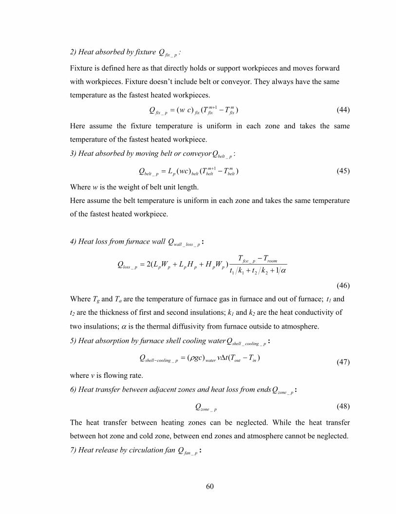
2) Heat absorbed by fixture : pfixQ _
Fixture is defined here as that directly holds or support workpieces and moves forward
with workpieces. Fixture doesn’t include belt or conveyor. They always have the same
temperature as the fastest heated workpieces.
)()( 1_
mfix
mfixfixpfix TTcwQ −= + (44)
Here assume the fixture temperature is uniform in each zone and takes the same
temperature of the fastest heated workpiece.
3) Heat absorbed by moving belt or conveyorQ : pbelt _
)()( 1_
mbelt
mbeltbeltppbelt TTwcLQ −= + (45)
Where w is the weight of belt unit length.
Here assume the belt temperature is uniform in each zone and takes the same temperature
of the fastest heated workpiece.
4) Heat loss from furnace wall Q : plosswall __
α1
)(22211
__ ++
−++=
ktktTT
WHHLWLQ roompfceppppppploss
(46)
Where Tg and Ta are the temperature of furnace gas in furnace and out of furnace; t1 and
t2 are the thickness of first and second insulations; k1 and k2 are the heat conductivity of
two insulations; α is the thermal diffusivity from furnace outside to atmosphere.
5) Heat absorption by furnace shell cooling waterQ : pcoolingshell __
)()(_ inoutwaterpcoolingshell TTtvgcQ −∆=− ρ (47)
where v is flowing rate.
6) Heat transfer between adjacent zones and heat loss from ends : pzoneQ _
pzoneQ _ (48)
The heat transfer between heating zones can be neglected. While the heat transfer
between hot zone and cold zone, between end zones and atmosphere cannot be neglected.
7) Heat release by circulation fan Q : pfan _
60

tT
HPQfce
fanpfan ∆
+⋅=
__ 460
520 (49)
where is the power of the fan. The same equation provided by Surface
Combustion.
fanHP
8) Heat input by the furnace : pfceQ _
tqKQ connAHpfce ∆⋅=_ (50)
5.8 Random Load Pattern
For random load pattern, it is limited to the load in the fixtures in the step by step
movement. There are two methods to calculate the heat transfer in the random load
pattern, the same as mentioned in the before reports [14]. The first method is the effective
thermal conductivity method, in which the effective thermal conductivity is first
calculated by experiment and inverse method and then is used to actual load. The second
method is the method based on the assumption of arranged load pattern. As the random
load pattern is assumed to be arranged together, then heat transfer can be calculated by
the method for arranged load pattern.
5.9 Output Results and Optimization of Furnace Control
5.9.1 Output results
As the calculation is finished, the following results are provided:
Temperature vs. time curves of each part in the calculation domain The temperature
of every workpiece in the calculation domain is calculated and output into text files.
The temperature of critical workpieces such as the fastest heated and slowest heated
workpieces can be directly plotted out after calculation.
The heat absorption rate of the calculated domain is calculated.
61
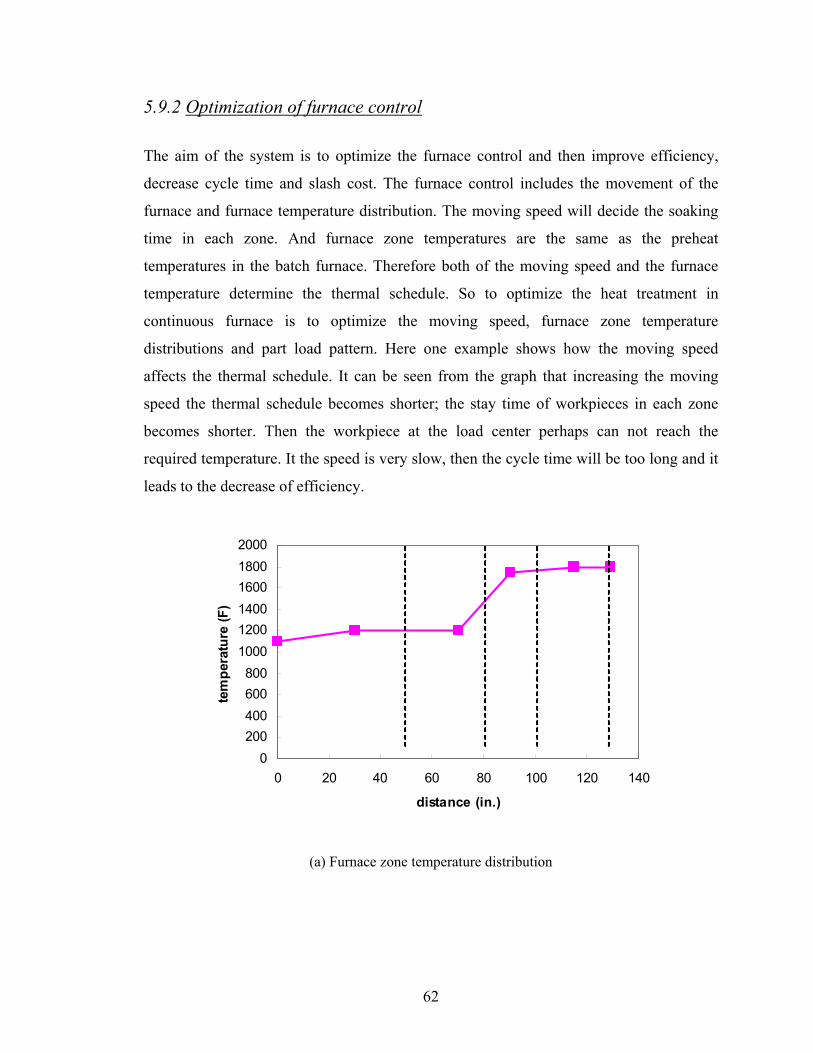
5.9.2 Optimization of furnace control
The aim of the system is to optimize the furnace control and then improve efficiency,
decrease cycle time and slash cost. The furnace control includes the movement of the
furnace and furnace temperature distribution. The moving speed will decide the soaking
time in each zone. And furnace zone temperatures are the same as the preheat
temperatures in the batch furnace. Therefore both of the moving speed and the furnace
temperature determine the thermal schedule. So to optimize the heat treatment in
continuous furnace is to optimize the moving speed, furnace zone temperature
distributions and part load pattern. Here one example shows how the moving speed
affects the thermal schedule. It can be seen from the graph that increasing the moving
speed the thermal schedule becomes shorter; the stay time of workpieces in each zone
becomes shorter. Then the workpiece at the load center perhaps can not reach the
required temperature. It the speed is very slow, then the cycle time will be too long and it
leads to the decrease of efficiency.
0200400600800
100012001400160018002000
0 20 40 60 80 100 120 140
distance (in.)
tem
pera
ture
(F)
(a) Furnace zone temperature distribution
62
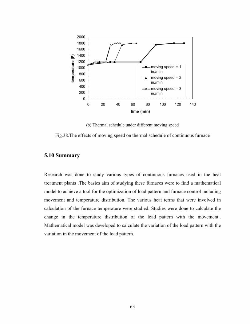
0200400600800
100012001400160018002000
0 20 40 60 80 100 120 140
time (min)
tem
pera
ture
(F)
moving speed = 1in./minmoving speed = 2in./minmoving speed = 3in./min
(b) Thermal schedule under different moving speed
Fig.38.The effects of moving speed on thermal schedule of continuous furnace
5.10 Summary
Research was done to study various types of continuous furnaces used in the heat
treatment plants .The basics aim of studying these furnaces were to find a mathematical
model to achieve a tool for the optimization of load pattern and furnace control including
movement and temperature distribution. The various heat terms that were involved in
calculation of the furnace temperature were studied. Studies were done to calculate the
change in the temperature distribution of the load pattern with the movement..
Mathematical model was developed to calculate the variation of the load pattern with the
variation in the movement of the load pattern.
63
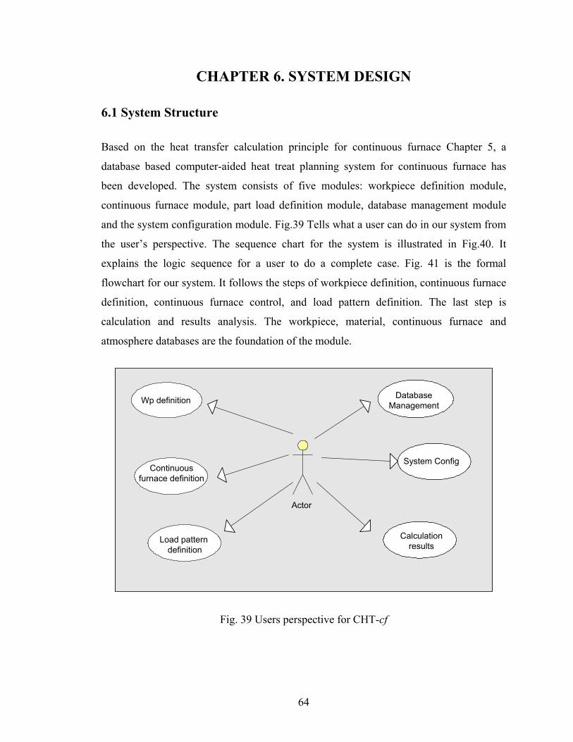
CHAPTER 6. SYSTEM DESIGN
6.1 System Structure
Based on the heat transfer calculation principle for continuous furnace Chapter 5, a
database based computer-aided heat treat planning system for continuous furnace has
been developed. The system consists of five modules: workpiece definition module,
continuous furnace module, part load definition module, database management module
and the system configuration module. Fig.39 Tells what a user can do in our system from
the user’s perspective. The sequence chart for the system is illustrated in Fig.40. It
explains the logic sequence for a user to do a complete case. Fig. 41 is the formal
flowchart for our system. It follows the steps of workpiece definition, continuous furnace
definition, continuous furnace control, and load pattern definition. The last step is
calculation and results analysis. The workpiece, material, continuous furnace and
atmosphere databases are the foundation of the module.
Continuousfurnace definition
Load pattern definition
Wp definition
Calculationresults
System Config
DatabaseManagement
Actor
Fig. 39 Users perspective for CHT-cf
64
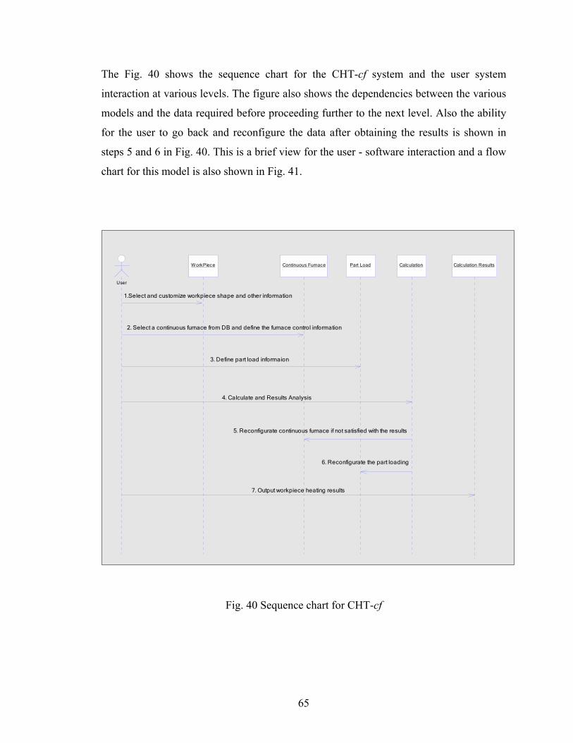
The Fig. 40 shows the sequence chart for the CHT-cf system and the user system
interaction at various levels. The figure also shows the dependencies between the various
models and the data required before proceeding further to the next level. Also the ability
for the user to go back and reconfigure the data after obtaining the results is shown in
steps 5 and 6 in Fig. 40. This is a brief view for the user - software interaction and a flow
chart for this model is also shown in Fig. 41.
1.Select and customize workpiece shape and other information
2. Select a continuous furnace from DB and define the furnace control information
3. Define part load informaion
4. Calculate and Results Analysis
5. Reconfigurate continuous furnace if not satisfied with the results
6. Reconfigurate the part loading
7. Output workpiece heating results
User
W orkPiece Continuous Furnace Part Load Calculation Calculation Results
Fig. 40 Sequence chart for CHT-cf
65
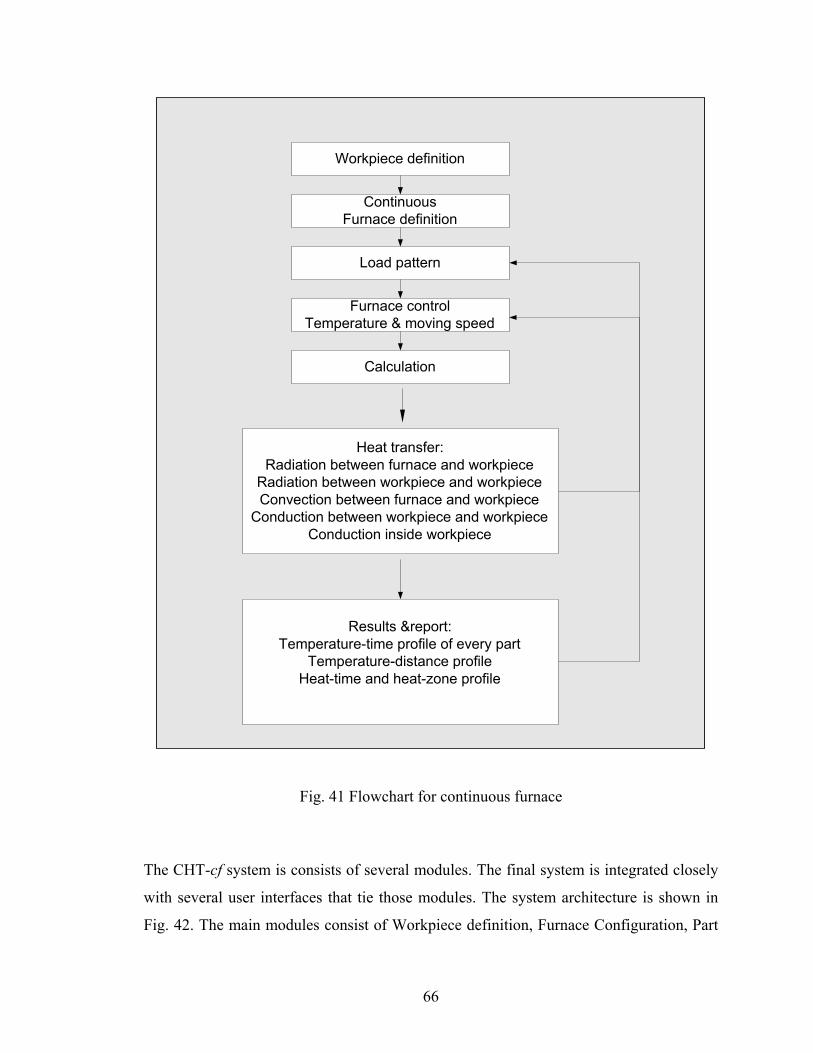
Workpiece definition
ContinuousFurnace definition
Load pattern
Furnace controlTemperature & moving speed
Calculation
Results &report:Temperature-time profile of every part
Temperature-distance profileHeat-time and heat-zone profile
Heat transfer:Radiation between furnace and workpiece
Radiation between workpiece and workpieceConvection between furnace and workpiece
Conduction between workpiece and workpieceConduction inside workpiece
Fig. 41 Flowchart for continuous furnace
The CHT-cf system is consists of several modules. The final system is integrated closely
with several user interfaces that tie those modules. The system architecture is shown in
Fig. 42. The main modules consist of Workpiece definition, Furnace Configuration, Part
66
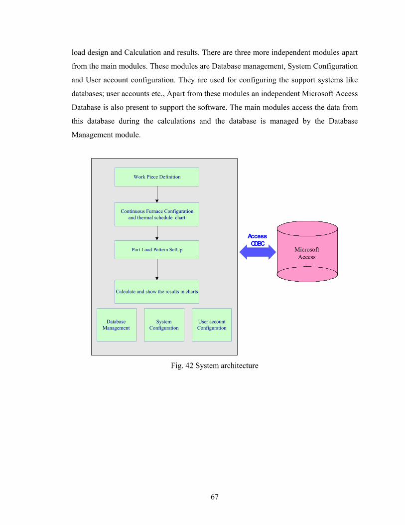
load design and Calculation and results. There are three more independent modules apart
from the main modules. These modules are Database management, System Configuration
and User account configuration. They are used for configuring the support systems like
databases; user accounts etc., Apart from these modules an independent Microsoft Access
Database is also present to support the software. The main modules access the data from
this database during the calculations and the database is managed by the Database
Management module.
Work Piece Definition
Continuous Furnace Configurationand thermal schedule chart
Part Load Pattern SetUp
Calculate and show the results in charts
DatabaseManagement
SystemConfiguration
User accountConfiguration
AccessODBC
MicrosoftAccess
Fig. 42 System architecture
67

6.2 Database Design for Continuous Furnaces
The database is the foundation of the system. Databases such as material, atmosphere and
fuel are the same as those for batch furnace. But the continuous furnace is different from
batch furnace, so the continuous furnace database is constructed. Fig.43 is the structure of
continuous furnace. It mainly includes the image path, type and zone information such as
length, temperature, horsepower of recirculation fan, atmosphere and etc. At most 10
zones are permitted in the database.
Fig. 43 Continuous furnace database structure
68
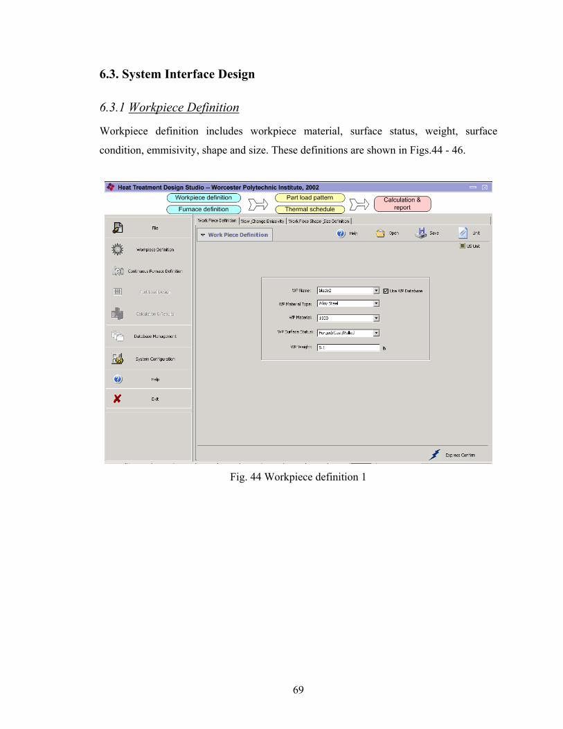
6.3. System Interface Design
6.3.1 Workpiece Definition
Workpiece definition includes workpiece material, surface status, weight, surface
condition, emmisivity, shape and size. These definitions are shown in Figs.44 - 46.
Fig. 44 Workpiece definition 1
69
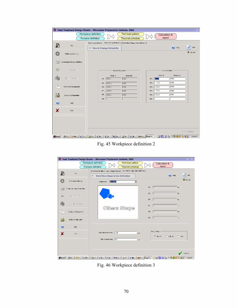
Fig. 45 Workpiece definition 2
Fig. 46 Workpiece definition 3
70
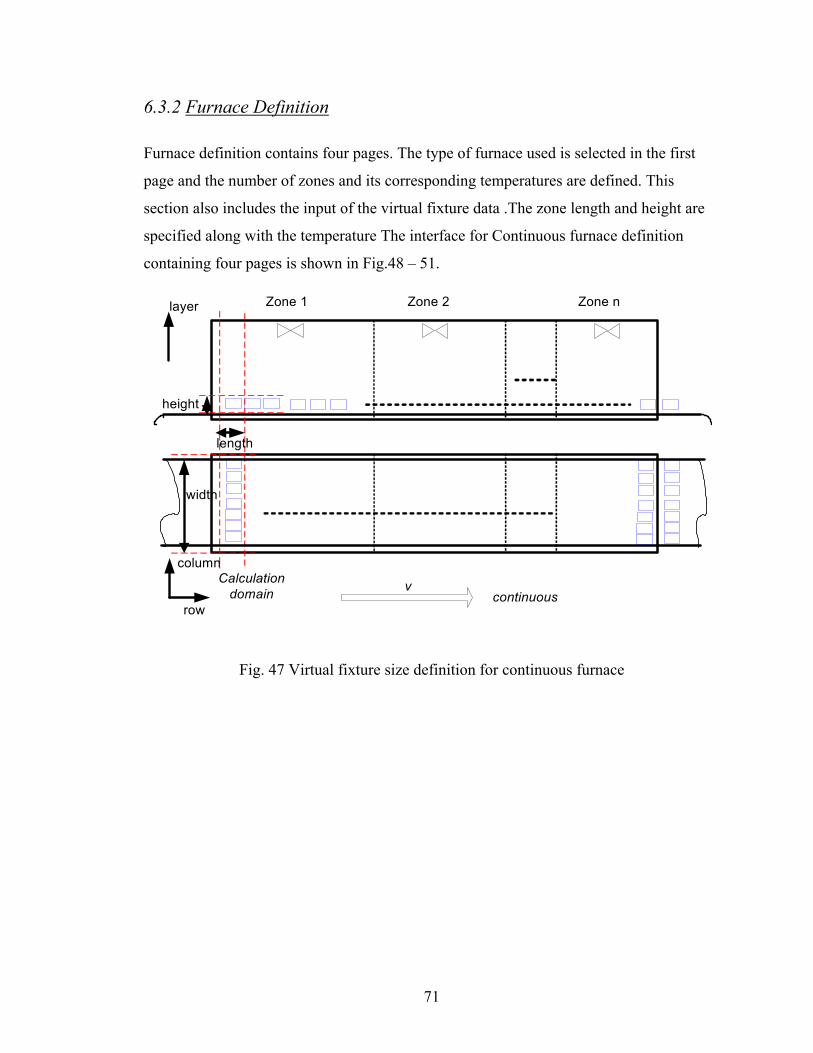
6.3.2 Furnace Definition
Furnace definition contains four pages. The type of furnace used is selected in the first
page and the number of zones and its corresponding temperatures are defined. This
section also includes the input of the virtual fixture data .The zone length and height are
specified along with the temperature The interface for Continuous furnace definition
containing four pages is shown in Fig.48 – 51.
Zone 1 Zone 2 Zone n
vcontinuous
Calculationdomain
row
column
layer
height
length
width
Fig. 47 Virtual fixture size definition for continuous furnace
71
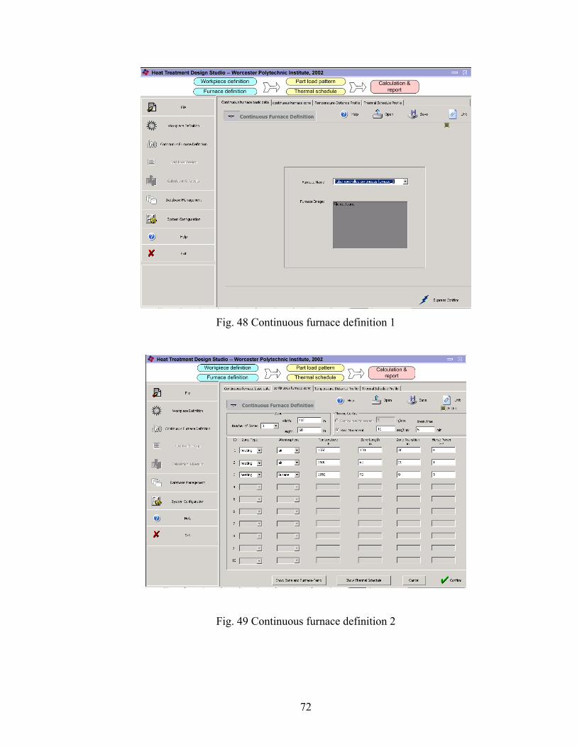
Fig. 48 Continuous furnace definition 1
Fig. 49 Continuous furnace definition 2
72
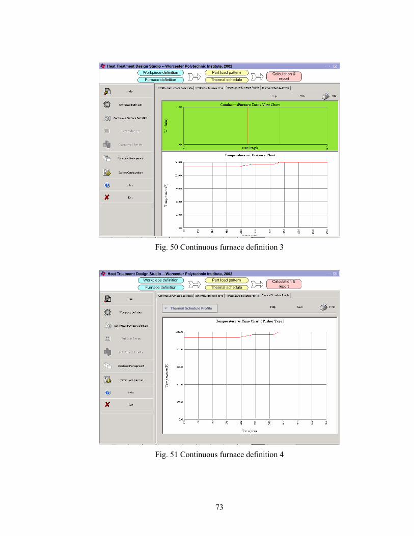
Fig. 50 Continuous furnace definition 3
Fig. 51 Continuous furnace definition 4
73

6.3.3 Load Pattern Definition
Load pattern consists of fixture configuration and the part configuration. Fixture
configuration consists of fixture shape and type. Part configuration consists of
arrangement of workpiece in the fixture, which can be aligned, staggered and random.
The load pattern definition is shown in Fig. 52.
Fig. 52 Load pattern definition
6.3.4 Results and Reports
The various results obtained from the system are shown in Fig. 53 and 54. Static curves
include the set zone temperatures in the furnace, furnace temperature, fastest workpiece
74
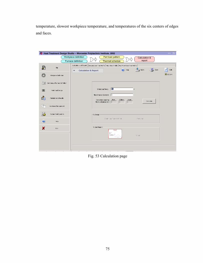
temperature, slowest workpiece temperature, and temperatures of the six centers of edges
and faces.
Fig. 53 Calculation page
75
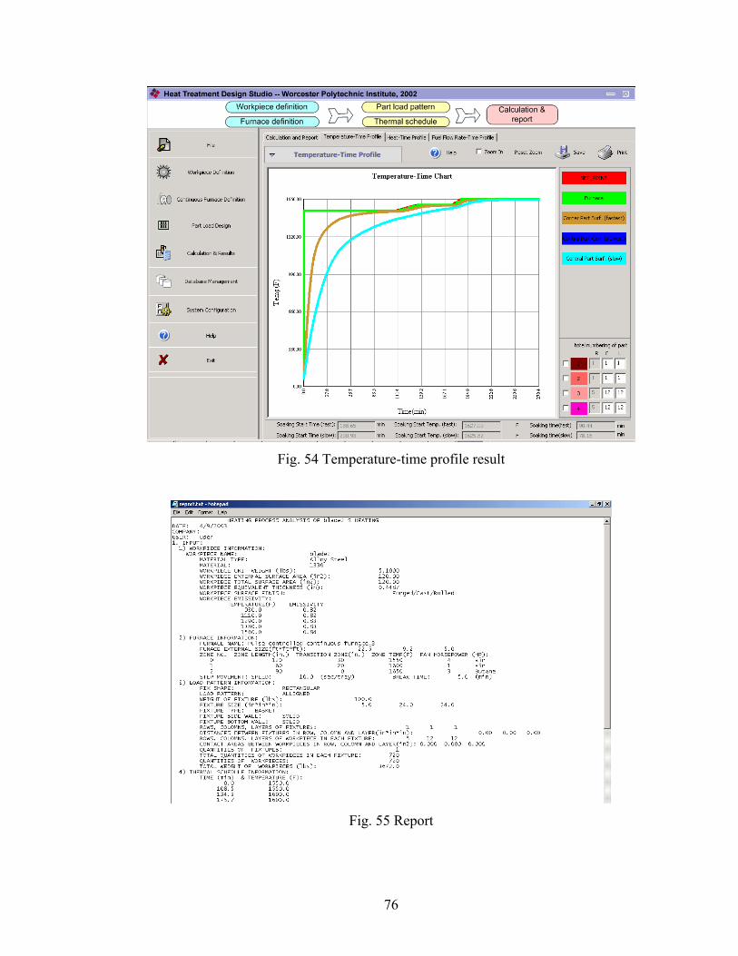
Fig. 54 Temperature-time profile result
Fig. 55 Report
76
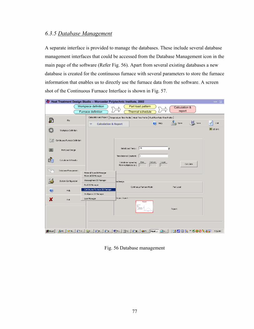
6.3.5 Database Management
A separate interface is provided to manage the databases. These include several database
management interfaces that could be accessed from the Database Management icon in the
main page of the software (Refer Fig. 56). Apart from several existing databases a new
database is created for the continuous furnace with several parameters to store the furnace
information that enables us to directly use the furnace data from the software. A screen
shot of the Continuous Furnace Interface is shown in Fig. 57.
Fig. 56 Database management
77
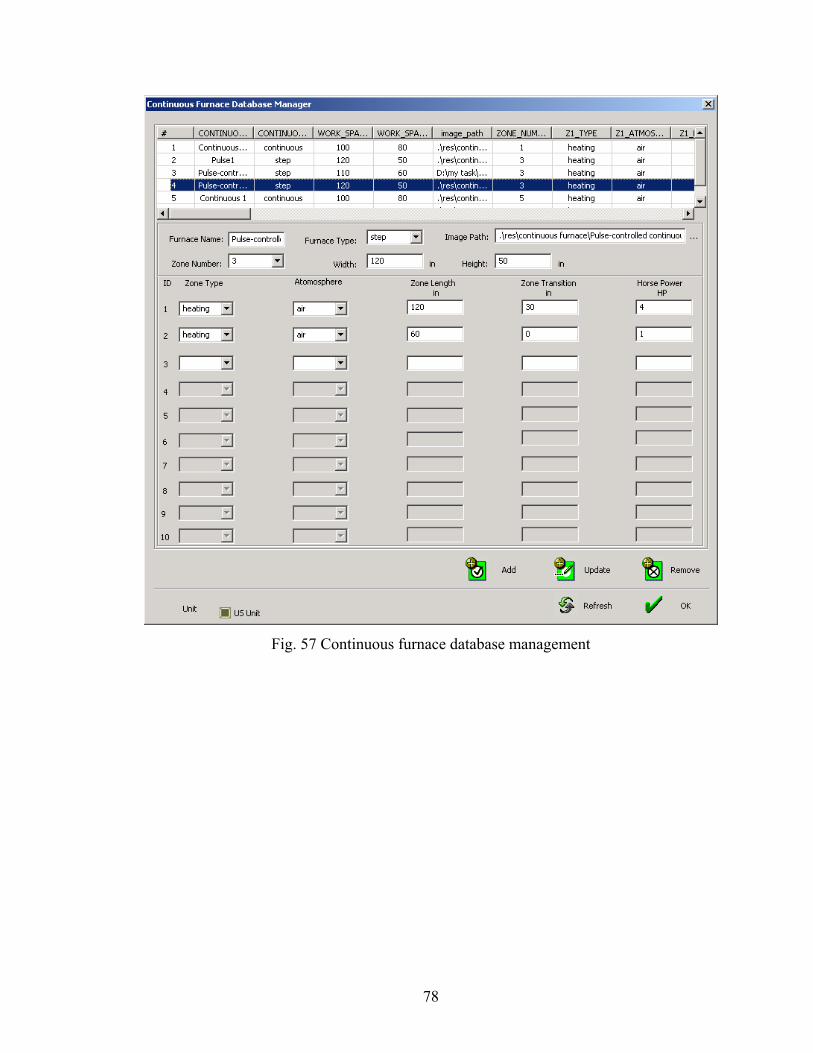
Fig. 57 Continuous furnace database management
78
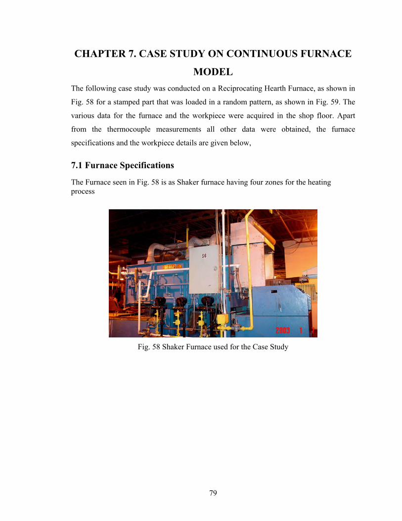
CHAPTER 7. CASE STUDY ON CONTINUOUS FURNACE
MODEL The following case study was conducted on a Reciprocating Hearth Furnace, as shown in
Fig. 58 for a stamped part that was loaded in a random pattern, as shown in Fig. 59. The
various data for the furnace and the workpiece were acquired in the shop floor. Apart
from the thermocouple measurements all other data were obtained, the furnace
specifications and the workpiece details are given below,
7.1 Furnace Specifications
The Furnace seen in Fig. 58 is as Shaker furnace having four zones for the heating process
Fig. 58 Shaker Furnace used for the Case Study
79
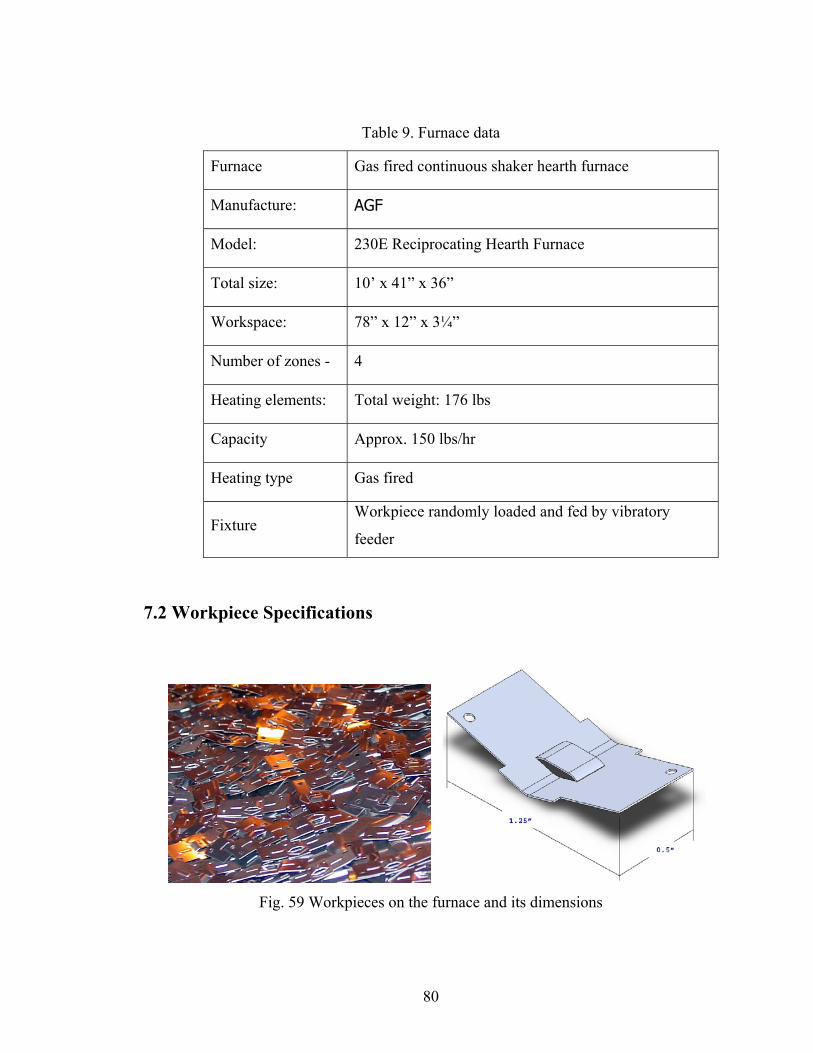
Table 9. Furnace data
Furnace Gas fired continuous shaker hearth furnace
Manufacture: AGF
Model: 230E Reciprocating Hearth Furnace
Total size: 10’ x 41” x 36”
Workspace: 78” x 12” x 3¼”
Number of zones - 4
Heating elements: Total weight: 176 lbs
Capacity Approx. 150 lbs/hr
Heating type Gas fired
Fixture Workpiece randomly loaded and fed by vibratory
feeder
7.2 Workpiece Specifications
Fig. 59 Workpieces on the furnace and its dimensions
80
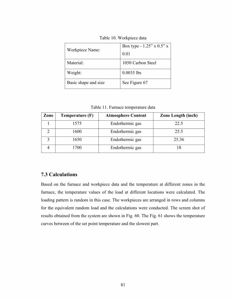
Table 10. Workpiece data
Workpiece Name: Box type - 1.25” x 0.5” x
0.01
Material: 1050 Carbon Steel
Weight: 0.0035 lbs
Basic shape and size See Figure 67
Table 11. Furnace temperature data
Zone Temperature (F) Atmosphere Content Zone Length (inch)
1 1575 Endothermic gas 22.5
2 1600 Endothermic gas 25.5
3 1650 Endothermic gas 25.36
4 1700 Endothermic gas 18
7.3 Calculations
Based on the furnace and workpiece data and the temperature at different zones in the
furnace, the temperature values of the load at different locations were calculated. The
loading pattern is random in this case. The workpieces are arranged in rows and columns
for the equivalent random load and the calculations were conducted. The screen shot of
results obtained from the system are shown in Fig. 60. The Fig. 61 shows the temperature
curves between of the set point temperature and the slowest part.
81
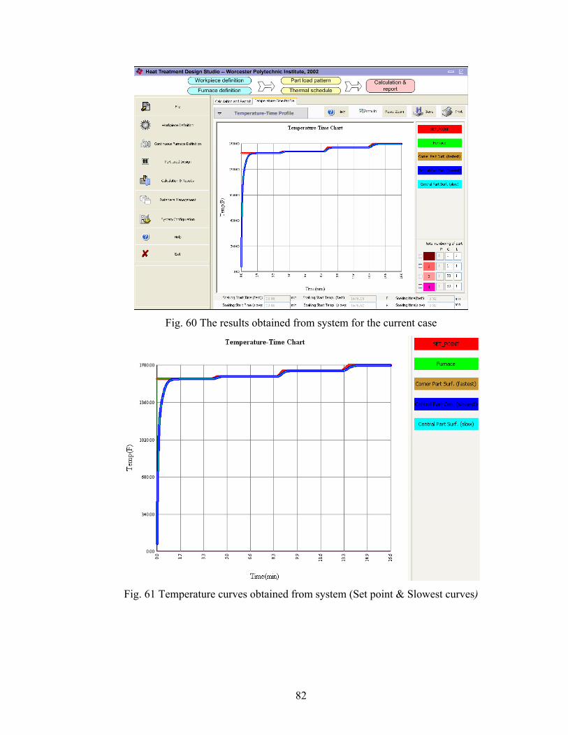
Fig. 60 The results obtained from system for the current case
Fig. 61 Temperature curves obtained from system (Set point & Slowest curves)
82

7.4 Results and Conclusions
As observed from the Fig. 61 for the temperature curve of the slowest curve there is some
room for improving the cycle time or the load pattern. But there are no measured results
available at this time to verify the system and calculated results. The case study is to be
continued. Once the data are obtained the system needs to be verified and further case
studies are required to validate the system under different conditions.
83

CHAPTER 8. SUMMARY
This thesis presented a Computerized Heat Treatment for batch (CHT-bf) with the
addition of random load model and for continuous furnace model CHT-cf. CHT is
developed to assist the heat treatment process. The temperature distribution inside the
furnace and the temperature of the various parts in the load can be determined. A number
of case studies were presented for the validation of the models. The prediction results of
workpiece temperature profiles are analyzed and compared with actual industrial results.
In the thesis, the following work has been done,
1. Physics-mathematical models, based on the heat transfer theory, for the random loads
were developed and various parameters are identified and classified.
2. There were basically two methods developed for the calculation of the effective
thermal conductivity of the random loads.
3. Case studies were conducted in order to test the accuracy of the system and to check
the random load model.
4. Further improvement was made in the database structure and the calculation process.
5. Mathematical model for the heat flow in the continuous furnace was developed.
6. A case study was conducted in order to check the system functionality of continuous
furnace and to study what future work would be needed for the improvement of the
system.
84
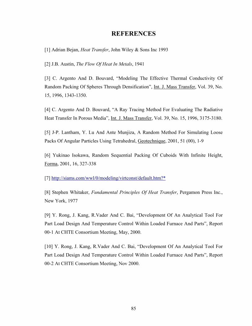
REFERENCES
[1] Adrian Bejan, Heat Transfer, John Wiley & Sons Inc 1993
[2] J.B. Austin, The Flow Of Heat In Metals, 1941
[3] C. Argento And D. Bouvard, “Modeling The Effective Thermal Conductivity Of
Random Packing Of Spheres Through Densification”, Int. J. Mass Transfer, Vol. 39, No.
15, 1996, 1343-1350.
[4] C. Argento And D. Bouvard, “A Ray Tracing Method For Evaluating The Radiative
Heat Transfer In Porous Media”, Int. J. Mass Transfer, Vol. 39, No. 15, 1996, 3175-3180.
[5] J-P. Lantham, Y. Lu And Ante Munjiza, A Random Method For Simulating Loose
Packs Of Angular Particles Using Tetrahedral, Geotechnique, 2001, 51 (00), 1-9
[6] Yukinao Isokawa, Random Sequential Packing Of Cuboids With Infinite Height,
Forma, 2001, 16, 327-338
[7] http://siams.com/wwl/0/modeling/virtconst/default.htm?*
[8] Stephen Whitaker, Fundamental Principles Of Heat Transfer, Pergamon Press Inc.,
New York, 1977
[9] Y. Rong, J. Kang, R.Vader And C. Bai, “Development Of An Analytical Tool For
Part Load Design And Temperature Control Within Loaded Furnace And Parts”, Report
00-1 At CHTE Consortium Meeting, May, 2000.
[10] Y. Rong, J. Kang, R.Vader And C. Bai, “Development Of An Analytical Tool For
Part Load Design And Temperature Control Within Loaded Furnace And Parts”, Report
00-2 At CHTE Consortium Meeting, Nov 2000.
85
[11] Y. Rong, J. Kang, R.Vader And C. Bai, “Development of an Analytical Tool for Part
Load Design and Temperature Control within Loaded Furnace and Parts”, Report 01-1 At
CHTE Consortium Meeting, May 2001.
[12] Y. Rong, Q. Lu, J. Kang And R. Vader, “Development Of An Analytical Tool For
Part Load Design And Temperature Control Within Loaded Furnace And Parts”, Report
01-2 At CHTE Consortium Meeting, Nov. 2001.
[13] Y. Rong, J. Kang, R.Vader And C. Bai, “Enhancement Of Computer-Aided Heat
Treating Process Planning System (CAHTPS)”, Report 02-1 At CHTE Consortium
Meeting, May 2002.
[14] Y. Rong, J. Kang, “Enhancement of Computer-Aided Heat Treating Process
Planning System (CAHTPS)”, Report 02-2 At CHTE Consortium Meeting, Nov 2002.
[15] Y. Rong, J. Kang, “Development of an Analytical tool for part load design and
temperature control in continuous furnace”, Report 03-1 At CHTE Consortium Meeting,
May 2003.
[16] H K. Nandi, M.C. Tomason and M.R. Delhuntly ‘Software Tool Optimizes Furnace
Design and operation,” Industrial Heat Progress, Nov 2002
[17] ICON and DCON Manual, GRI and Purdue Univ, 1995
[18] D O. Marlow “Modeling Direct-Fired Annealing Furnace For Transient operation,”
Appl Math.Modeling, 20, 35-40 (1996).
[19] K S. Chapman, S Ramadhyani, R.Viskanta, “Modeling And Analysis Of Heat
Transfer In A Direct-Fired Continuous Reheating Furnace.”
86