Enhanced-resolution lidar

1044 J. Opt. Soc. Am. A/Vol. 14, No. 5 /May 1997 Bas et al.

Enhanced-resolution lidar

Christophe F. Bas, Timothy J. Kane, and Christopher S. Ruf

The Communications and Space Sciences Laboratory, The Pennsylvania State University,316 Electrical Engineering East, University Park, Pennsylvania 16802-2707

Received March 28, 1996; revised manuscript received October 31, 1996; accepted November 8, 1996

To retrieve a high-resolution vector signal from a set of measured low-resolution vector signals, we deliberatelydelayed the synchronization between the transmitter and the receiver of a pulsed laser radar (lidar). Onceseveral range-shifted low-resolution vector signals had been obtained, we independently applied a regulariza-tion method and the singular-value-decomposition method to restore high-resolution characteristics. Theformer approach remains preferable when the signal-to-noise ratio is low, whereas the latter provides resultssimilar to those of the former, but with lesser effort, as the signal-to-noise ratio becomes high. © 1997 OpticalSociety of America [S0740-3232(97)00205-6]

1. INTRODUCTIONThe field of image processing has shown that blurred,noisy, and randomly space-shifted series of images couldbe satisfactorily recovered by using methods either in thespace domain or in the wave-number domain.1 Success-ful restoration of this inverse problem can be performedthrough regularization techniques,2,3 which require somestatistical knowledge of the image and its associatednoise. The Wiener filter4–7 is a particular type of regu-larization filter.Instead of taking a bidimensional image, pulsed laser

radars (lidars) capture a vector signal of the environmentwith each shot. Assuming that this environment re-mains static (often referred to as frozen), a delay of thesynchronization between the transmitter and the receiverprovides information complementary to that of the initialpulse. The low-resolution vector signals obtained fromthe emission of several desynchronized pulses form acomplete set of measurements whose inverse reconstructsa high-resolution vector signal. When the effect of noiseis important, better results are provided by the regular-ization method than by the unconstrained restorationtechniques. However, when the effect of noise is small,unconstrained restoration methods deliver satisfactoryresults while diminishing the complexity of the calcula-tions.The compromise among the validity of the static-

environment supposition, the high frequencies of interest,and the maximum sampling rate obtainable with avail-able devices determines the optimum number of pulsesnecessary to make a complete set of measurements.Section 2 elaborates on the proposed technique to re-

trieve high-resolution signals and Section 3 sets up a deg-radation model. Section 4 focuses on the restorationmethods, Section 5 provides examples, and Section 6 con-cludes this paper.

2. TECHNIQUELidars8 include two entities: a transmitter and a re-ceiver. The transmitter sends a narrow pulse that trav-

0740-3232/97/0501044-07$10.00 ©

els at almost c ' 3 3 108 m/s. Every location illumi-nated by the pulse scatters toward the receiver someinformation that is processed and delivered as a discretesignal of finite length: a low-resolution signal of dimen-sion 1 3 M. The system requires a dwell-time period ofT seconds per element (also called bin, channel, or pixel).Synchronization between the two entities ensures thatthe location of the source of information is known at alltimes within T 3 c meters. Our objective is to provide ahigh-resolution signal whose dimension is 1 3 (MN1 N 2 1), where N is the spatial amplification factor,reducing the imprecision to within T 3 c/N m.Toward this aim, and toward the construction of one

complete set of measurements, N periodic pulses need tobe transmitted, each of which is shifted in time by T/Nwith respect to the actual synchronization instant of theprevious pulse, as shown Fig. 1. The consequence of thistechnique is, as illustrated in Fig. 2, to allow for the use ofthe same degradation model for either photon-counting orlow-pass-filter-equipped sampling devices (in which casethe degradation matrix HNTI defined later needs to be di-vided by the period T).

3. DEGRADATION MODELThe degradation model is expressed as

zNTI 5 yNTI 1 n, (1)

with

yNTI 5 HNTIx t, (2)

where yNTI 5 @y1 y2 y3•••yM# t is the column vectormade of the low-resolution vector signals obtained by suc-cessive pulses; x is the high-resolution vector signal thatwe hope to retrieve; n is the contribution of noise through-out the system and modeled as additive, white, andGaussian with zero mean; and HNTI is the degradationmatrix whose dimension is (MN) 3 (MN 1 N 2 1),whose structure follows from the technique used therein:

1997 Optical Society of America

Bas et al. Vol. 14, No. 5 /May 1997/J. Opt. Soc. Am. A 1045

HNTI 5 310A000A000A0

10A010A000A0

•••

•••

•••

•••

•••

•••

•••

•••

•••

10A010A010A0

01A010A010A0

01A001A010A0

•••

•••

•••

•••

•••

•••

•••

•••

•••

01A001A001A0

00A001A001A0

00A000A001A0

•••

•••

•••

•••

•••

•••

•••

•••

•••

00A100A100A0

00A100A100A0

00A000A100A0

•••

•••

•••

•••

•••

•••

•••

•••

•••

00A000A000A1

00A000A000A1

00A000A000A1

4 . (3)

Although HNTI does not display the property of time invariance (which is at the origin of its subscript), it is possible torestructure the matrix so that it does. We shall call this new matrix HTI , which is obtained by writing yTI 5 HTIx t,where (see Fig. 2)

HTI 5 F 100A0

110A0

111A0

•••

•••

•••

•••

111A0

011A0

001A0

000A0

•••

•••

•••

•••

000A0

000A1

000A1

000A1

•••

•••

•••

•••

000A1

G (4)

and yTI 5 @y1,1 y2,1 y3,1 ••• yN,1 y1,2 ••• yN,2 y1,3 ••• y1,M y2,M ••• y1,M# t.The previous result is generalized as yTI(k) 5 hTI(k) * x(k), where * denotes the convolution operator and

Fig. 1. Illustration of the technique used to obtain a high-resolution vector signal from N low-resolution vector signals. The periodicthick lines at the emitter represent the time of emission of a pulse, whereas the actual recording time at the receiver begins at Ts1 ^i&N 3 (T/N), where Ts is the nominal synchronization time, i is a natural number, and ^i&N is the value of i modulo N.

Fig. 2. When three pulses are sent (N 5 3), the corresponding three low-resolution vector signals (y1 , y2 , and y3) form a complete setof measurements. All low-resolution vector signals are related to the high-resolution vector signal x through the time-shift technique.


hTI~k ! 5 H1 for k 5 0, 1, 2...N 2 10 otherwise , (5)

whose frequency domain counterpart is

HTI@exp~ jvT !# 5 exp@2jvT~N 2 1 !/2#sin~vTN/2!

sin~vT/2!.

(6)

We conclude that the recovery (which makes use ofHNTI) will not be successful for frequencies at and aroundthose for which HTI@exp( jvT)# 5 0. Hence one muststrongly consider the range of frequencies of interest be-fore choosing N.

4. RESTORATIONWe seek a way to compute xNTI

t 5 H21zNTI while control-ling the effect of the noise in our ill-posed inversion. xdenotes one of the possible high-resolution vector signals.The expression for H21 is the topic of this section. Twosolutions are suggested, the selection of which is moti-vated by the value of the signal-to-noise ratio (SNRz) es-timated from the low-resolution vector signals.In the regularized underconstrained inverse (RUI) ap-

proach, we restrict ourselves to the minimization of thefollowing function:

iy 2 HNTIxi2 1 gixi2, (7)

where small values for g give an emphasis to the datapoints, whereas large values promote a smooth result forthe estimation of the high-resolution vector signal.9 Theresulting solution2,3 is found to be

H21 [ HNTIt ~HNTIHNTI

t 1 gI!21, (8)

where g 5 C/SNRz and I is the identity matrix. The realconstant C was determined for the simulated signals ofSection 5 by selecting the C that minimized the meansquare error (MSE) between the known low-resolutionvector signal y and HNTIx, the degraded version of the re-stored high-resolution vector signal, for which g is used.Wahba10 suggested practical means to evaluate g fromnoisy data.If the effect of the noise is small, g in Eq. (8) becomes so

small that it is tempting to write H21[ HNTIt

3 (HNTIHNTIt )21, the underconstrained inverse.6,11

Nonetheless, this last equation and H21 5 HNTI21 , solved

through the singular value decomposition (SVD) method,lead to the same results. SVD has been chosen overother unconstrained methods because of its simplicity, ef-ficiency, and beauty. The SVD principle resides in thedecomposition of a matrix of arbitrary dimensions intothe product of three matrices: HNTI 5 U S V t, whereS is a diagonal matrix whose diagonal elements (singularvalues) are either positive or zero and U t U 5 V t V5 1. A carefree inversion of HNTI gives

HNTI21 5 @U S V t#21

5 @V t#21 S21 U21

5 V S21 U t, (9)

where the last line is obtained by using the orthonormalproperty of both V and U. One advantage of SVD is to

signal any problems by inserting zeros on the diagonal ofS. Since the degradation shows a loss of N 2 1 dimen-sions, we expect to find N 2 1 zero singular values (thedimension of HNTI is MN 3 MN 1 N 2 1, forcing therank of H21 to be MN). One commonly accepted meansto compute S21 is to let the zero singular values of S re-main zero in S21 while forcing the values that are smallenough in S21 to introduce some instability to zero inS21. Press et al.11 provide both an overview of the SVDmethod and an algorithm that generates U, S, and V.We conclude that the high-resolution restored vector

signal xNTIt is obtained by multiplying H21 by zNTI .

5. EXAMPLESTo illustrate the results of the technique presentedherein, we provide two examples, both of which start withartificially generated high-resolution vector signals.

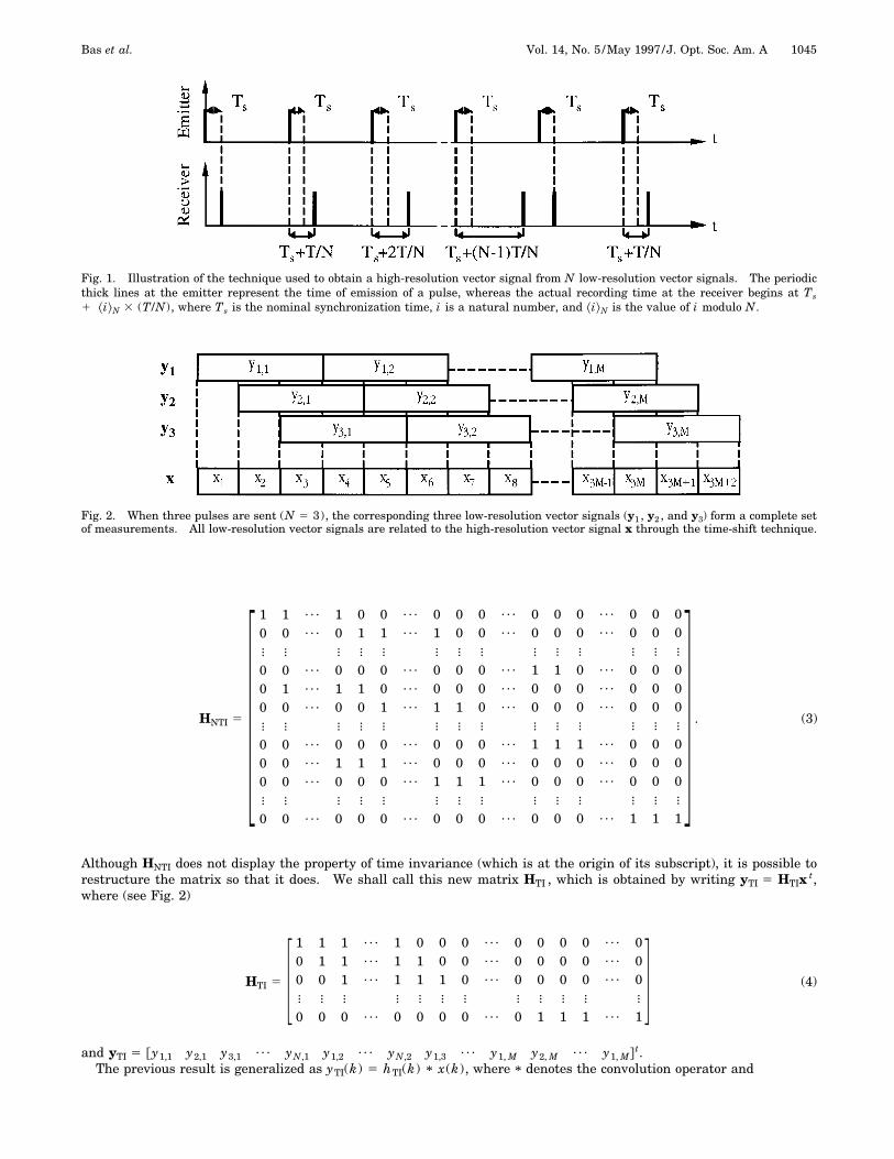
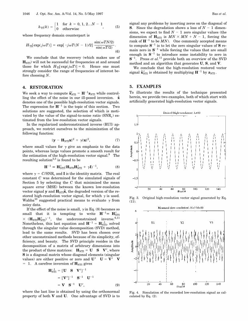
Fig. 3. Original high-resolution vector signal generated by Eq.(11).

Fig. 4. Simulation of the recorded low-resolution signal as cal-culated by Eq. (2).


The degradation model first computes the low-resolution vector signal [Eq. (2)], followed by the noise ad-dition [Eq. (1)]. Then the restoration model consists inthe multiplication of the result of Eq. (1) by H21 to obtainthe estimated high-resolution vector signal. Comparisonbetween the restored high-resolution vector signal andthe original one is done by calculation of the MSE, whoseexpression is

MSE 51

MN 1 N 2 1 (i51

MN1N21

@ x~i !NTI 2 x~i !original#2

(10)

for RUI and SVD reconstructions, both of which provideMN 1 N 2 1 high-resolution pixels. Some figures usethe SNR that is calculated for z, the noisy low-resolutionvector signal.

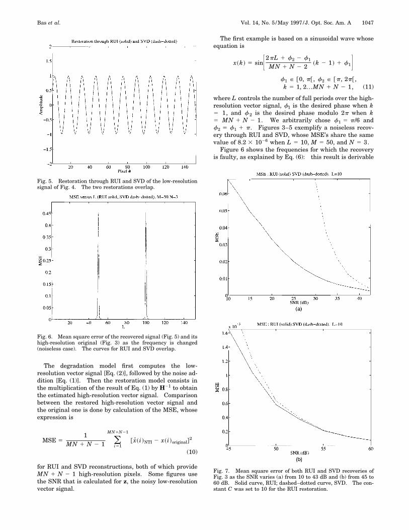
Fig. 5. Restoration through RUI and SVD of the low-resolutionsignal of Fig. 4. The two restorations overlap.

Fig. 6. Mean square error of the recovered signal (Fig. 5) and itshigh-resolution original (Fig. 3) as the frequency is changed(noiseless case). The curves for RUI and SVD overlap.

The first example is based on a sinusoidal wave whoseequation is

x~k ! 5 sinF2pL 1 f2 2 f1

MN 1 N 2 2~k 2 1 ! 1 f1G

f1 P @0, p@ , f2 P @p, 2p@ ,k 5 1, 2...MN 1 N 2 1, (11)

where L controls the number of full periods over the high-resolution vector signal, f1 is the desired phase when k5 1, and f 2 is the desired phase modulo 2p when k5 MN 1 N 2 1. We arbitrarily chose f1 5 p/6 andf2 5 f1 1 p. Figures 3–5 exemplify a noiseless recov-ery through RUI and SVD, whose MSE’s share the samevalue of 8.2 3 1026 when L 5 10, M 5 50, and N 5 3.Figure 6 shows the frequencies for which the recovery

is faulty, as explained by Eq. (6): this result is derivable

Fig. 7. Mean square error of both RUI and SVD recoveries ofFig. 3 as the SNR varies (a) from 10 to 43 dB and (b) from 45 to60 dB. Solid curve, RUI; dashed–dotted curve, SVD. The con-stant C was set to 10 for the RUI restoration.


by solving V 3 N/2 5 np for L while rejecting those forwhich V/2 5 mp, where both n and m are integer num-bers and V 5 (2pL1 f2 2 f1)/(MN 1 N 2 2). TheSNR is given by the ratio of the average power of the low-resolution signal to the variance of the noise at the samelocation:

SNRdB 5 10 log10H 1

2sn2 F sin~NV/2!

sin~V/2!G2J , (12)

where sn2 is the variance of the degraded noise [Brown

and Hwang5 provide a method for obtaining Eq. (12)].Figure 7 plots MSE versus SNRdB . As N is increased(keeping about the same dimension for the high-resolution vector signal) the number of frequencies thatare not recoverable increases, therefore increasing theMSE. Hence the smaller N, the smaller the MSE for agiven SNR. A plot addressing this point is presented

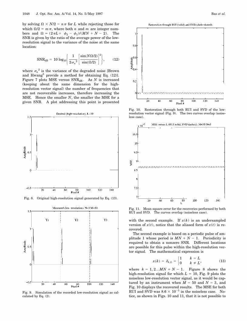
Fig. 8. Original high-resolution signal generated by Eq. (13).

Fig. 9. Simulation of the recorded low-resolution signal as cal-culated by Eq. (2).

with the second example. If x(k) is an undersampledversion of x(t), notice that the aliased form of x(t) is re-covered.The second example is based on a periodic pulse of am-

plitude 1 whose period is MN 1 N 2 1. Periodicity isrequired to obtain a nonzero SNR. Different locationsare possible for this pulse within the high-resolution vec-tor signal. The mathematical expression is

x~k ! 5 dk,L 5 H10 k 5 Lk Þ L, (13)

where k 5 1, 2...MN 1 N 2 1. Figure 8 shows thehigh-resolution signal for which L 5 10, Fig. 9 plots thenoiseless low-resolution vector signal, as it would be cap-tured by an instrument when M 5 50 and N 5 3, andFig. 10 displays the recovered results. The MSE for bothRUI and SVD was 8.6 3 1025 in the noiseless case. No-tice, as shown in Figs. 10 and 11, that it is not possible to

Fig. 10. Restoration through both RUI and SVD of the low-resolution vector signal (Fig. 9). The two curves overlap (noise-less case).

Fig. 11. Mean square error for the recoveries performed by bothRUI and SVD. The curves overlap (noiseless case).


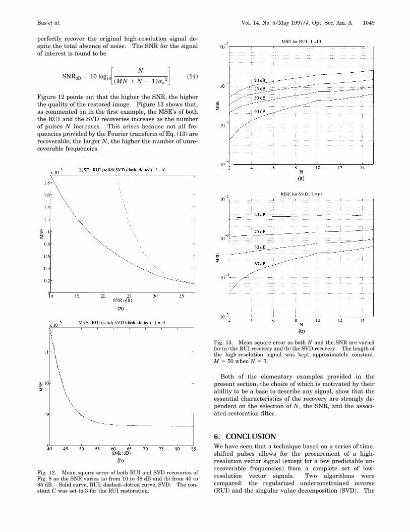
perfectly recover the original high-resolution signal de-spite the total absence of noise. The SNR for the signalof interest is found to be

SNRdB 5 10 log10F N

~MN 1 N 2 1 !sn2G . (14)

Figure 12 points out that the higher the SNR, the higherthe quality of the restored image. Figure 13 shows that,as commented on in the first example, the MSE’s of boththe RUI and the SVD recoveries increase as the numberof pulses N increases. This arises because not all fre-quencies provided by the Fourier transform of Eq. (13) arerecoverable; the larger N, the higher the number of unre-coverable frequencies.

Fig. 12. Mean square error of both RUI and SVD recoveries ofFig. 8 as the SNR varies (a) from 10 to 38 dB and (b) from 40 to85 dB. Solid curve, RUI; dashed–dotted curve, SVD. The con-stant C was set to 3 for the RUI restoration.

Both of the elementary examples provided in thepresent section, the choice of which is motivated by theirability to be a base to describe any signal, show that theessential characteristics of the recovery are strongly de-pendent on the selection of N, the SNR, and the associ-ated restoration filter.

6. CONCLUSIONWe have seen that a technique based on a series of time-shifted pulses allows for the procurement of a high-resolution vector signal (except for a few predictable un-recoverable frequencies) from a complete set of low-resolution vector signals. Two algorithms werecompared: the regularized underconstrained inverse(RUI) and the singular value decomposition (SVD). The

Fig. 13. Mean square error as both N and the SNR are variedfor (a) the RUI recovery and (b) the SVD recovery. The length ofthe high-resolution signal was kept approximately constant.M 5 50 when N 5 3.


former provided more robust answers when the SNR ofthe collected data was low, but the quality of the recoveryit provided was comparable to that of SVD as the SNR in-creased to become significantly high.We noticed that the smaller the number of low-

resolution vector signals needed to make a complete set ofmeasurements, the better. The dynamics of the probedenvironment, the frequencies of interest, and the avail-ability of the hardware should also be considered.One among the several applications this technique of-

fers is an increase of accuracy in target ranging.

ACKNOWLEDGMENTSThe authors thank the reviewer for providing construc-tive suggestions. This research was supported in part bythe Department of Electrical Engineering at The Pennsyl-vania State University and NASA grant NAG5-5035.

REFERENCES1. M. K. Ozkan, A. T. Erdem, M. I. Sezan, and A. M. Tekalp,

‘‘Efficient multiframe Wiener restoration of blurred andnoisy image sequences,’’ IEEE Trans. Image Process. 1,453–476 (1992).

2. A. N. Tikhonov and V. Y. Arsenin, Solutions of Ill-posedProblems (Wiley, New York, 1977).

3. M. Bertero, ‘‘Linear inverse and ill-posed problems,’’ in Ad-vances in Electronics and Electron Physics, Peter W.Hawkes, ed. (Academic, San Diego, Calif., 1989), Vol. 75.

4. R. C. Gonzalez and R. E. Woods, Digital Image Processing(Addison-Wesley, Reading, Mass., 1992).

5. R. G. Brown and P. Y. C. Hwang, Introduction to RandomSignals and Applied Kalman Filtering (Wiley, New York,1992).

6. A. Gelb, J. F. Kasper, Jr., R. A. Nash, Jr., C. F. Price, and A.A. Sutherland, Applied Optimal Estimation (MIT Press,Cambridge, Mass., 1974).

7. H. L. van Trees, Detection, Estimation and ModulationTheory. Part I: Detection (Wiley, New York, 1968).

8. R. M. Measures, Laser Remote Sensing: Fundamentalsand Applications (Krieger, Malabar, Fla., 1992).

9. J. B. Abiss and B. J. Brames, ‘‘Restoration of sub-pixel de-tail using the regularized pseudo-inverse of the imaging op-erator,’’ in Advanced Signal Processing, Architectures andImplementations II, F. T. Luk, ed., Proc. SPIE 1566, 365–375 (1991).

10. G. Wahba, ‘‘Practical approximate solutions to linear opera-tor equations when the data are noisy,’’ SIAM J. Numer.Anal. 14, 651–667 (1977).

11. W. H. Press, S. A. Teukolsky, W. T. Vetterling, and B. P.Flannery, Numerical Recipes in C (Cambridge U. Press,Cambridge, 1992).

Documents

Enhanced-resolution lidar