Enhanced Possibilities for Analyzing Tree Structure as ...wkurth/cb/html/dzierzon_sf.pdf · Enhanced Possibilities for Analyzing Tree Structure as Provided by an Inter-face between

31

Enhanced Possibilities for Analyzing Tree Structure as Provided by an Inter-face between Different ModellingSystems

Helge Dzierzon, Risto Sievänen, Winfried Kurth, Jari Perttunen and Branislav Sloboda

Dzierzon, H., Sievänen, R., Kurth, W., Perttunen, J. & Sloboda, B. 2003. Enhanced possibilities for analyzing tree structure as provided by an interface between different modelling systems. Silva Fennica 37(1): 31–44.

In recent years, many different advanced mathematical models and simulation systems for tree and forest growth have been developed. We show a possibility to extend analysis tools for measured and simulated plants using a data interface between the simulation model LIGNUM and the multifunctional software system GROGRA. Both systems were developed by different teams. To demonstrate the enhanced possibilities for analyzing a LIGNUM tree, several examples are given. In these examples three different approaches for analysis are applied to measured and simulated trees: Fractal dimension, deduction of tapering laws, and water potential patterns obtained from simulation of waterflow by the specialized software HYDRA. Conclusions for the interfacing and comparison of different modelling tools are drawn.

Keywords mathematical models, simulation systems, tree growth, forest growth, analysis toolsAuthors´ addresses Dzierzon & Sloboda: Institut für Forstliche Biometrie und Informatik, Universität Göttingen, Büsgenweg 4, D-37077 Göttingen, Germany; Sievänen & Pert-tunen: The Finnish Forest Research Institute, Vantaa Research Centre, P.O. Box 18, FIN-01301 Vantaa, Finland; Kurth: Institut für Informatik, Brandenburgische Technische Universität Cottbus, P.O. Box 101344, D-03013 Cottbus, GermanyE-mail [email protected] Internet http://www.uni-forst.gwdg.de/~wkurth/plant.htmlReceived 9 October 2001 Accepted 4 November 2002

Silva Fennica 37(1) research articles

1 IntroductionTo enhance understanding and prediction of tree and forest growth, many different mathemati-cal models and simulation systems have been

developed, reaching from classical yield tables to process-based models. The latter usually try to capture the dynamics of carbon fluxes between compartments of the trees, like the collection of all leaves, the bole, the root system (e.g. McMurtrie

32


and Wolf 1983; see Mäkelä et al. 2000 for a recent overview). However, in heterogeneous stands, the competitive success of a tree depends to a large extent on the three-dimensional distribution of its biomass and that of the competitors, and therefore on morphological properties. Plants show plasti-city of form and changing carbon allocation pat-terns in response to environmental differences. During the last years it has become evident that a precise description of the morphological con-struction of the growing tree and its competitive environment, and a linkage between structural and process-based components, are required for modelling tree growth (Bassow et al. 1990). The result were so-called functional-structural tree models (FSTMs) (Perttunen et al. 1996, Kurth and Sloboda 1997, Reffye et al. 1997, Balandier et al. 2000, Bosc 2000, Eschenbach 2000, Jallas et al. 2000, Sievänen et al. 2000) which treat morphological entities of a tree as interacting units, each equipped with its own geometrical, physical and physiological characteristics. They are becoming increasingly popular as research tools in botany, agronomy and forest science. The representation of tree architecture in FSTMs requires (at least implicitly) some mathematical concepts for handling branched, multiscaled structures (e.g. list representations, L-systems, graph theory; cf. Godin and Caraglio 1998). The model LIGNUM (Perttunen et al. 1996, 1998) is an example of an FSTM.

The result of a simulation run with a FSTM is usually a large 3-D structure with numerous components, each of them characterized by many values of variables. If one wants to compare such a virtual tree structure with a real tree or with the result of another model, some tools for analyzing tree representations should be at hand.

The software GROGRA (Kurth 1994, 1999) provides several analysis tools of that kind. GROGRA was originally developed to create tree structures specified by L-systems. To enable the validation and comparison of model results, vari-ous algorithms for analyzing branching systems were implemented in the same software. It would be possible to reimplement these algorithms in LIGNUM, but we considered it as more effi-cient to use an existing software. Therefore we designed a data interface between LIGNUM and GROGRA. In this paper we describe the construc-

tion of this interface and demonstrate some of the possibilities for analyzing tree structures which arise from this connection by applying a collec-tion of different methods. Interfaces can also be used for linking models (Anzola 2002). But the aim of this interface is comparing model results to aid model validation or model fitting processes. Exemplarily, we perform an estimation of box counting dimension, we analyze branch tapering (cross section area / supported biomass-relation-ship), and we apply a specialized physical model simulating water flow and distribution of water potentials in the tree crown. In addition to the tree simulated by LIGNUM, we use for our analysis also tree structures obtained directly from detailed measurements of some sample trees.

2 Interfacing LIGNUM and GROGRA

2.1 LIGNUM

The structural representation of a tree with LIGNUM can be formally defined as follows (cf. Fig. 1):

The model tree of LIGNUM consists of one axis. An axis is a possibly empty sequence of tree segments (TS), branching points (BP) and exactly one bud (B) terminating the sequence.

Fig. 1. The structure of a LIGNUM tree.TS = Tree segment, BP = Branching point, B = Bud.

33

Dzierzon, Sievänen, Kurth, Perttunen and Sloboda Enhanced Possibilities for Analyzing Tree Structure as Provided by an Interface …

Each tree segment must be followed by exactly one branching point. A branching point is a set of zero or more axes.

The definition does not imply how LIGNUM should be implemented. The current implementa-tion as a list of lists is one possibility. However, the definition sets the requirement that the units appear in the axis in a certain order: tree segments and branching points occur alternatingly and the bud is the rearmost unit. There can also be an axis containing only one bud. The definition of the branching point simply captures the branched structure of the tree.

A tree segment corresponds to a piece (seg-ment) of a woody axis, containing heartwood, sapwood, bark and possibly foliage. Coniferous and deciduous trees are distinguished. Tree seg-ments of conifers contain a cylinder of needles and have buds at the end. The segments of deciduous trees have individual leaves and buds. An axis is a sequence of segments and branching points terminating in a bud. Axes correspond to the stems and branches of real trees. Branching points can be thought of as points that connect branches (axes) to the stem or higher order branches in real trees. The tree itself is thus an aggregation of its axes (Perttunen et al. 1996). The roots are considered only in terms of their mass. The metabolic functioning (e.g. photosynthesis and respiration) and the physiological state of the units are directly associated to them.

LIGNUM simulates the interception of photo-synthetically-active radiation (PAR) in the tree crown, photosynthesis as conversion of radia-tion to dry matter, respiration, and the allocation of carbon among the tree segments. Secondary growth of the woody axes is mainly controlled by the necessity to maintain sufficient sapwood area for hydraulic supply of the supported foliage. The number and length of new shoots growing each year is determined by the available amount of carbon and by species-specific morphogenetic patterns.

In this case we used LIGNUM to simulate Scots pine (Pinus sylvestris L.) trees, i.e. conifers. Hence a tree segment contains sap- and heart-wood, bark and needles. The relative thickness growth of the woody parts of branches is based on the pipe model (Shinozaki et al. 1964). Used parameters are listed in Table 1. The parameters are the same as in Perttunen et al. (1998) except a new component within the light model, which mimics a surrounding tree stand.

The radiation model is a central part of LIGNUM and it treats attenuation of solar radia-tion in the crown of the tree itself, i.e. self shad-ing. The amount of light which reaches a tree segment has two components in calculation. First, the sky is divided into sectors and the amount of radiation coming from each sector during the growing period is assumed to be known (Perttunen et al. 1998). The amount of radiation

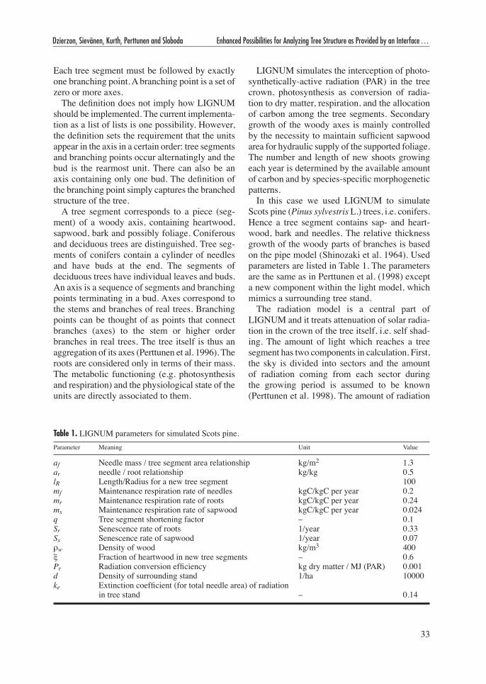
Table 1. LIGNUM parameters for simulated Scots pine.Parameter Meaning Unit Value

af Needle mass / tree segment area relationship kg/m2 1.3ar needle / root relationship kg/kg 0.5lR Length/Radius for a new tree segment 100mf Maintenance respiration rate of needles kgC/kgC per year 0.2mr Maintenance respiration rate of roots kgC/kgC per year 0.24ms Maintenance respiration rate of sapwood kgC/kgC per year 0.024q Tree segment shortening factor – 0.1Sr Senescence rate of roots 1/year 0.33Ss Senescence rate of sapwood 1/year 0.07ρw Density of wood kg/m3 400ξ Fraction of heartwood in new tree segments – 0.6Pr Radiation conversion efficiency kg dry matter / MJ (PAR) 0.001d Density of surrounding stand 1/ha 10000ke Extinction coefficient (for total needle area) of radiation in tree stand – 0.14

34


coming from each sector is calculated from zonal brightness of standard overcast sky (Ross 1981). In the simulations, the total incoming radiation was 1200 MJ/m2 of photosynthetically active radiation during growing season corresponding to conditions in southern Finland (Stenberg 1996). Second, the beam of light coming from a sky sector may go through foliage or hit the woody part of a segment in the tree crown. If it hits the woody part, it is blocked. The attenuation caused by foliage is calculated according to Oker-Blom and Smolander (1988), see also Kellomäki and Strandman (1995). For further information we refer to Perttunen et al. (1998).

In the simulations, the surrounding stand was treated in a simplified manner. It was assumed that the simulated tree grows among identical trees in a homogeneous stand (i.e. the trees in the surrounding stand grow at the same rate as the simulated tree). The attenuation of radiation in the surrounding stand was exponential:

qr = e–ke · dist · needle_dens (1)

where qr is the relative intensity of the beam after travelling distance dist in the stand which has needle density needle_dens, and extinction coefficient, ke.

2.2 GROGRA

The software GROGRA (“Growth Grammar interpreter”; Kurth 1994, 1999) was primarily designed as a system for the interpretation of extended L-systems. L-systems (Lindenmayer systems; named after the botanist Aristid Linden-mayer, 1925–1989) are systems of replacement rules which allow a precise and condensed speci-fication of architectural growth rules of branching organisms. GROGRA was specifically tailored to the simulation of forest trees in ecophysiologi-cal applications. (There exist other L-system softwares, e.g., L-Studio/cpfg; Prusinkiewicz et al. 2000). Beyond the pure grammar interpreta-tion, GROGRA provides additional features which form our main focus of interest here: A data filter to represent measured trees, interfaces linking it to process-oriented simulation tools and to statistical software (Fig. 2), and analysis tools. An overview of analysis options available with GROGRA is given in Table 2; more detailed information can be found in Kurth (1994, 1999) and on the GROGRA web page 1).

This design of GROGRA allows the representa-tion of L-system-generated and manually-meas-ured trees in the form of the same data structure

Fig. 2. Structure of the software GROGRA. The grey zone denotes the GROGRA kernel.

1) http://www.uni-forst.gwdg.de/~wkurth/grogra.html

35


and their comparison with the same analysis tools (see Kurth 1999 for examples of Norway spruce trees). This internal structure is a linked tree of records (cf. Godin 2000), which is not very differ-ent from LIGNUMʻs internal tree representation. It was our motivation here to extend the possi-bilities of precise comparison and analysis of virtual tree structures to trees generated by other growth simulation models (here, LIGNUM) as well. No use was made of the L-system specific components of GROGRA, which are devoted to synthesis of trees rather than analysis.

2.3 Implementation of the Interface

Both LIGNUM and GROGRA treat a simulated tree in a very detailed way. Detailed means that the software treats information on organ level though other models are even more detailed according to physiological and multiscaled infor-

mation. The information of interest in a simulated tree is stored in LIGNUM as well as in GROGRA in a data type which basically represents the organ “tree segment”. The task was to collect the tree segments out of a LIGNUM tree and to filter the data which they contain to make them readable for GROGRA.

For translating trees from LIGNUM to GROGRA it is necessary to consider two items: The information stored in tree segments itself, and how those segments are linked together, i.e. the representation of topology.

The representation of topology in both tools is different. Hence we need a translation process. Focussing on a segment GROGRA stores infor-mation in the data structure of the segment about location of the segment within the tree architec-ture. Every segment “knows” its predecessor, that is, mother segment. The segments altogether are chained in a list. The list itself does not represent the context of tree segments. But the “knowl-

Table 2. Analysis options implemented in GROGRA.

Elementary gives fundamental parameters: number of elementary units, number of terminal units, total length, volume, surface area and others – available for the simulated structure as a whole and for individual plants

Distribution frequency tables: elementary units, compound units, axes, el. units per compound unit etc., in total and for each branching order

Table for each elementary unit (shoot): identifyer, id. of mother unit, number of daughter units, length, diameter, branching angle, squared sum of daughter diameters and other parameters, suitable for processing with statistical software

Topological number of components, number of (graph-theoretical) links, maximal and average topological depth and other topological parameters, see Oppelt et al. (2001)

Pathlength table enabling analysis of diameter-pathlength relation according to McMahon and Kronauer (1976) and other approaches for tapering

Cubic cells rasterization of leaf area suitable for interfacing with turbid-medium radiation simulators (see Kurth 1999 for details)

Fractal rasterization with varying grid resolution, yields data file for further processing with box-counting analysis software (cf. Oppelt et al. 2000)

Bole table with discretized description of the main stemLevel total length and leaf area included in horizontal layers with specified thicknessBranch for each elementary unit: number of daughter units and their positions (for further processing) positionsAxes parameters for each axis, including average interbranch distance and its standard deviationPopulation time series of frequencies of elementary units of different types dynamicsHYDRA rediscretization interface for processing with water flow simulator HYDRA (Früh 1995)

36


edge” of mother segments satisfies the minimum demands posed by representing topology.

The data structure of LIGNUM represents topol-ogy in a more direct way. As already described, tree segments are merged in lists, which describe axes in the systematic of Gravelius order (cf. Fig. 1). It is quite complex to query such a data structure. In our case we have to calculate the mother segments for each segment. If one would scan tree segment by tree segment through this list of lists, it is not guaranteed the predecessor element is the mother segment – usually it is not. LIGNUM offers algorithms to solve such problems. One allows querying the structure considering the topology. At a branching point the algorithm allows to treat daughter segments in a quasi simultaneous way. This allows to pass the information “who is the mother” to the daughter segments.

The information of a tree segment can be subdivided into three parts: identification, geo-metrical and physiological information. In the filtering process information can take three ways: direct adoption, transformation, and sometimes information has to be calculated newly out of existing data.

An important difference between LIGNUM and GROGRA is the amount of physiological information. GROGRA is basically confined to morphological data but LIGNUM stores physi-ological and other data of each segment. Table 3 shows the physiological information which LIGNUM holds in a segment. GROGRA provides space for five unspecified variables which can be used for whatever information is required. One way to solve this problem was to make it optional which parameters shall be converted.

The converter translates the LIGNUM tree directly into a GROGRA 3D structure (cf. Fig. 2). Technically the converter uses the LIGNUM libraries to build up a LIGNUM tree. That means that the converter is part of the LIGNUM software family and stores the result of conversion in a so called “DTG file”. This is an ASCII-file which can be read by GROGRA.

3 Material and Methods3.1 Sample Trees

As reference trees which can be compared with simulated ones, three Scots pine trees (Pinus sylvestris L.) were investigated. The trees were 8, 10 and 11 years old; they were grown on a poor sandy (medium new red sandstone) soil in a wide-spaced stand together with some aged pine trees, located in Reinhausen near Göt-tingen (Germany). The trunk and the complete above-ground branching system of each tree was mapped; lengths, diameters, angles and positions of insertion nodes of each growth unit were manu-ally measured and recorded in a DTD file (Kurth 1994), together with the topological information necessary to reconstruct the structure of the tree crown. As we have used these trees only as exam-ples and not to deduce general statements about Scots pine, we will present only results obtained from one of them in the following sections. The results from the other two trees were similar to the presented ones in all cases.

The appearance of the analyzed trees is shown in Fig. 3. The real pine (left side) is the 11 years old measured one, hence we simulated a pine with a (fictitious) age of 11 years (right side). As the measured trees grew within a stand, we adopted the light regime in simulations to correspond to a stand consisting of identical trees.

Table 4 gives some characteristics of analyzed trees. Trees marked with bold font are used in the examples.

Table 3. Selection of physiological information of a LIGNUM tree segment.

Part of physiological information stored in a LIGNUM tree segment

Foliage massSapwood massDry weightRespiration rateRadius of heartwood

37


3.2 Used Methods of Analysis and Simulation

The purpose of interfacing the software systems was to extend possibilities of analysing trees cre-ated by one specific software (LIGNUM) without programming new tools but by using existing components from other software systems. To give an impression of the resulting possibilities, we apply exemplarily three methods of analysis:1) Estimation of fractal dimension,2) analysis of diameters,3) simulation of water flow by HYDRA (Früh 1995).

3.2.1 Fractal Analysis

One of our example methods is fractal analysis of branching systems. The estimation of the fractal dimension (meaning a possibly non-integral number between 0 and 3) of a natural object can be considered as a way to quantify how intensely the object fills the space in which it is embedded (Mandelbrot 1982, Voss 1988). The fractal dimen-sion of a living organism is regarded to stand in connection with its gas exchange, biomechanical and transport characteristics (West et al. 1997,

Fig. 3. The shape of the investigated trees. Left: real Scots pine. Right: a Scots pine tree simulated by LIGNUM. Visualization of the above-ground tree skeleton without foliage, provided by GROGRA.

Table 4. Some characteristics of the analyzed trees.Characteristics of trees Real pine 3 Real pine 2 Real pine 1 Simulated pine

Age, years 10 8 11 11Height, cm 138.02 203.44 115.50 170.60Diameter of first element, cm 3.12 1.91 1.80 1.74Volume of stem, cm3 438.58 371.58 149.75 158.47

38


1999). Various definitions of “dimension” and “fractal” are used in the mathematical literature (see Edgar 1990, Peitgen et al. 1992). Here we restrict ourselves to box counting dimension as the most commonly used variant for botanical objects (Stoll 1995, Berntson and Stoll 1997, Oppelt et al. 2000). Basically, it describes the relationship between the number of equal-sized cubic cells or boxes needed to cover the whole object when it is embedded in a 3-D grid and the resolution at which the object is observed, i.e. the side length of the boxes. When resolution varies between specific upper and lower bounds (outer and inner cutoff, cf. Berntson and Stoll 1997), a linear regression between log(resolution) and log(box count) can be established in many cases. The negative slope of this regression line esti-mates the fractal dimension of the object under consideration. The closer this value comes to 3, the stronger the space-filling tendency of the object. To get a visual impression of this approach, we refer to Kurth (1999) and to the examples given below (Fig. 4). However, box-counting dimension concentrates structural properties of a tree in only one value, disregarding architectural differences e.g. between branches of different age and order; its descriptive power is therefore limited. Other methods of analysis, yielding different informa-tion, will be explained below.

Box counting dimension was estimated for the skeletons of the tree crowns, using a fixed set of grid resolutions: 200, 180, 160, 140, 120, 100, 80, 60, 50, 40, 30 and 20 mm, which is identical with the set used by Petermann (1999) for young Norway spruce trees. This set of resolutions covers approximately the range of size relevant for the proper branching systems of the trees. Par-ticularly, structures below 20 mm (“inner cutoff”), like, e.g., surface features of single shoots, are not considered. The existence of outer and inner cutoff distinguishes fractal analysis of real-world structures from ideal mathematical fractals which typically exhibit self-similarity at arbitrary scales (Berntson and Stoll 1997). Estimation of box counting dimension was carried out by simple linear regression analysis of logarithmic resolution and frequency values obtained from GROGRA analysis data (regression calculations done with the software tool GRODISC, cf. Dzi-erzon and Kurth 2002).

3.2.2 Analysis of Diameters

For analysing diameters we took as an example a relationship proposed by Chiba (1990, 2000) on the basis of the pipe model theory of trees (Shi-nozaki et al. 1964). He hypothesized that the total weight T distal to a position z should be directly supported by stem biomass per length, S, at that position. This relationship is supposed to have a linear form. Hence we get approximatively:

T(z) = b · S(z) (2)

where b is a proportionality constant (cf. Chiba 2000). In the examples we inserted for S the cross-sectional area of a segment and for T the accumulated weight of all tree segments (includ-ing leaves) distal to the considered one.

3.2.3 Simulation of Water Flow

In contrast to the statistical methods of analysis mentioned above, the simulation of tree-internal water flow with the software HYDRA (Früh 1995, Früh and Kurth 1999) follows a physical, mechanistic approach. The numerical algo-rithms in HYDRA are based on a discretized initial boundary value problem (cf. Douglas and Jones 1963) combining Darcy flow in the branched network of woody axes, water storage and conductivity losses due to cavitation events. By a sound mathematical derivation and by model tests, a consistent translation of the physiologi-cal assumptions into the computational kernel of HYDRA was ensured (Früh and Kurth 1999). The necessary structural information (topology and geometry of branches, leaf distribution) is taken from GROGRA, using a data filter which ensures the fulfillment of numerical require-ments imposed upon the spatial discretization of the tree crown by performing a fusion of closely neighbouring branching nodes and by insertion of additional, intermediate nodes (see Kurth 1994 and Früh 1995 for details). Time series of tran-spiration and soil water potential are also input of HYDRA and can be taken from measurements or from separate models.

In contrast to other models of the tree as a hydraulic system (e.g. Tyree and Sperry 1988,

39


Rapidel 1995), HYDRA does not only calculate steady-state distributions of water potential and flows, but allows short-term dynamic studies concerning the response of the system to sudden changes in the transpiration rate (Früh and Kurth 1999). However, here we will restrict ourselves to simulated steady-state profiles of water poten-tial along selected paths in the crown. This sort of output allows to find out in which branches the lowest potentials occur, and to assess the hydraulic significance of crown architecture by comparing profiles obtained from systematically varied branching systems.

Current limitations of HYDRA are the assump-tion of a uniform transpiration rate throughout the whole crown, the missing connection to leaf energy balance and stomatal regulation, and the lack of a feedback to a model of water transport in the soil. All these issues are currently being addressed (Lanwert et al. 1998).

4 ResultsThe results presented here are to be understood as examples indicating the possibilities originating from interfacing the two software systems.

4.1 Fractal Analysis

Fig. 4 shows the results of fractal analysis. Each of the trees shows fractal behaviour. The real Scots pine has a dimension of around 1.24. That of the simulated one is practically the same (1.27). The low values (< 2) result from our exclusion of foliage and from our choice of outer and inner cutoff. So, the two branching systems are “not far” from linear structures (dimension 1) in the considered range of grid resolutions.

4.2 Analysis of Diameters

Fig. 5 shows the results of analysis of supplied mass of a tree segment. S is the basal area of a segment, T the accumulated mass of the segments supplied by the considered segment (cf. Chiba 2000). The range of S and T is nearly the same in both cases but the shape of the scatterplot is different. The relationship was supposed to have a linear form, but the simulated pine seems to exhibit a nonlinear shape which we fitted tenta-tively by a quadratic polynomial.

4.3 Simulation of Water Flow

Fig. 6 shows the results of simulation of water flow. In this simulation we used an empirical relationship between the diameter d of a segment

Fig. 4. Results of fractal analysis. Left: real Scots pine. Right: simulated Scots pine. s = grid resolution, N = number of occupied grid cells. cd = coefficient of determination

40


and its hydraulic conductivity HC (cf. Cochard, 1992). The relationship is

HC = 3.715 · d2.41 (3)

for Scots pine. HYDRA (Früh, 1995) gives a diagram of water potential [MPa] versus path length [m] as possible output. Before start-ing the simulation, paths have to be selected. HYDRA calculates among others the water potential within all segments. The graphical output uses only preselected paths to prevent confusion. To give an overview about simulated waterflow within the trees, paths were selected which represent all branching orders in the tree.

Another term of selection was the location within the tree. We tried to select paths which represent different locations. The longest path is the main stem (branching order 0). Along a path, the order usually changes. Hence the marked orders in Fig. 6 are the orders of the last segment.

5 Discussion and ConclusionsInterfaces between software tools for creating, analyzing and manipulating virtual plants are useful for comparison of model results with field data and to test theoretical analysis approaches.

Fig. 5. Results of analysis of supplied biomass. Left: real Scots pine. Right: simulated Scots pine. S = cross section area of segment, T = accumulated biomass of all segments distal to the considered one, cd = coefficient of determination.

Fig. 6. Water potential versus distance from base of the tree along preselected paths with different values of branching order, in the simulated (A) and real (B) tree. The order of a path is determined by the order of its last segment.

41


An exchange of data between software systems broadens the spectrum of available methods for validation and comparison between models. Because different teams of researchers have their specific views and approaches, an exchange of data and the application of tools developed by another team can help to detect weaknesses of specific models which are easily overlooked by one team alone. The accessibility of a larger database of plant architectures (measured and simulated) will also provide better possibilities to validate functional-structural tree models. Our study describes how an interface between differ-ent tools can be constructed, shows exemplarily some of the possibilities of data analysis but also pinpoints some of the difficulties which can arise when different research tools for plant structures are interfaced.

The main technical problem was to specify an appropriate filter which makes data from LIGNUM accessible for GROGRA. Because GROGRA provides less physiological infor-mation than LIGNUM, there is no one-to-one correspondence between the elementary data structures of both softwares, although they are very similar in their way to represent tree architecture. However, the unavoidable loss of information did neither affect the application of analysis methods included in the GROGRA system, nor did it interfere with the hydraulic simulation performed with HYDRA on the basis of GROGRA structures.

Results were presented which imply a com-parison between a simulated and a real Scots pine tree. These comparisons were not designed to verify or falsify the LIGNUM model for Scots pine. The measured sample trees were from a site in Germany, whereas LIGNUM was parameter-ized for trees grown in Finland, i.e. under dis-tinctly different climatic conditions. Furthermore, our comparisons were not systematical enough: A larger number of sample trees would have been necessary to yield statistically secure results. This tentative study was only meant to demonstrate some of the possibilities which are opened by interfacing different software tools. Other inter-faces, e.g. between GROGRA and AMAPmod (Godin et al. 1998) provide even more pos-sibilities to analyze LIGNUM-generated trees (Dzierzon and Kurth 2002). Another task for the

future should be the quantification of differences between model results. Especially the results of water flow are difficult to compare.

Zeide and Pfeifer (1991) found values of frac-tal dimension greater than two and lower than three measured at Rocky Mountains conifers in South Carolina (USA). Their values are thus much larger than ours. Unfortunately it is not possible to compare these results directly. Zeide and Pfeifer (1991) used a so called “two surface method” to calculate what they denoted as “fractal dimension”. This method differs strongly from the box counting method and uses differences in the sizes of the given trees as the only source of variation of scale. Another difference is that we only calculated the dimension of the tree skeleton without leaves (needles). Furthermore our investi-gated trees are much smaller. Zeide s̓ and Pfeifer s̓ trees have diameters greater than 5 cm compared to ours with a maximum diameter of 3.12 cm (cf. Table 4).

In simulation-derived water potential profiles, there was again a high degree of qualitative similarity between simulated and architecturally-measured trees (we emphasize that we did not measure the water potentials directly). Quantita-tive differences were, like in diameter analysis, mainly due to differences in the distribution of diameters along the woody axes: The tree simu-lated by LIGNUM had a relatively weak second-ary growth. This explains also the low simulated water potential values: HYDRA uses an empiri-cally-derived diameter-conductivity relationship where the diameter of a segment appears in the formula with an exponent of 2.41 (from Cochard 1992). Therefore, a small reduction of diameter can already cause a considerable reduction of axial hydraulic conductivity, which will normally lead to lower potentials during simulation.

In Chiba s̓ (1990, 2000) cross-section area vs. biomass relationship test (Fig. 5), the results of measured and simulated trees differed. The differ-ence between the shapes of the curves was mainly caused by segments belonging to the main stem of the tree. Nevertheless, this difference is remark-able, since Chiba s̓ approach and the mechanistic growth model of LIGNUM (see Perttunen et al. 1996) were both inspired by the “pipe model” of Shinozaki et al. (1964). In the analysis of Chiba, the total cross-sectional area of stem and branches

42


were used. LIGNUM employs a stipulation of the pipe model (Nikinmaa 1992) in which the cross-sectional area of sapwood instead of total cross-sectional area is used. According to Fig. 5, Chiba s̓ interpretation of the pipe model seems to correspond to the data of this study better than that used in LIGNUM. This analysis shows that caution has to be applied when general ideas like the “pipe model” are used in specific models. A specification of complex models, like models of carbon alloca-tion in trees, must therefore be precise and should not rely on ambiguous terms like “pipe model”. Such a term can be understood and applied in many ways (e.g. for a tree as a whole or for junctions of tree parts as in LIGNUM). It should also be kept in mind that the observed crown level or branch level pipe model relationships are also affected by the rate of senescence of the foliage and by heartwood formation. The effects of heartwood formation have been studied in the framework of LIGNUM (Sievänen et al. 1997).

We compared results of HYDRA visually – i.e. in a qualitative and limited way of comparison. To go one step further would mean to quantify the differences, that is, to calculate distances between two simulations of water potential in tree crowns. It is not an easy task to define such distance meas-ures. A purely graph-theoretical distance like that proposed by Ferraro and Godin (2000) for plant architecture is not sufficient because the sizes of the water potential gradients play also an impor-tant role in our case. Perhaps a combination of graph-theoretical and physical distances would have to be defined and applied here.

Bridges between different software systems can help to spare much time which is normally necessary to implement a simulation model or generic analysis tools. Systems like AMAPmod, LIGNUM or HYDRA have cost many man-years to develop them, and sharing their use is therefore a question of economy in research. On the other hand, it is also clear that learning and under-standing a specific method can be much more thorough if a research team manages to create its own software tool incorporating the method and experiences the intrinsic difficulties of the method during the process of software development and debugging. Here, a balance between both require-ments – economy and “learning by doing” – has to be found by each team.

Acknowledgements

This study has been supported by the Deutsche Forschungsgemeinschaft (DFG; grant no. KU 847/3-1 and SL 11/7-3), by the DAAD (grant no. D/99/02585) and by the Academy of Finland (grant no. 50183). Michael Schulte and Olaf Oliefka have harvested and digitized the sample trees. All support is gratefully acknowledged.

ReferencesAnzola, G. 2002. Linking structural and process-

oriented models of plant growth. Dissertation, University of Göttingen, 166 p.

Balandier, Ph., Lacointe, A., Le Roux, X., Sinoquet, H., Cruiziat, P. & Le Dizès, S. 2000. SIMWAL: A structural-functional model simulating single walnut tree growth in response to climate and prun-ing. Annals of Forest Science 57(5/6): 571–585.

Bassow, S.L., Ford, E.D. & Kiester, A.R. 1990. A critique of carbon-based tree growth models. In: Dixon, R.K., Meldahl, R.S., Ruark, G.A. & Warren, W.G. (eds.). Process modeling of forest growth responses to environmental stress. Timber Press, Portland, 50–57.

Berntson, G.M. & Stoll, P. 1997. Correcting for finite spatial scales of self-similarity when calculating the fractal dimensions of real-world structures. Pro-ceedings of the Royal Society. London. (Series) B 264: 1531–1537.

Bosc, A. 2000. EMILION, a tree functional-structural model: Presentation and first application to the analysis of branch carbon balance. Annals of Forest Science 57(5/6): 555–569.

Chiba, Y. 1990. Plant form analysis based on the pipe model theory. I. A statical model within the crown. Ecological Research 5: 207–220.

— 2000. Mathematical model of stem formation and tree architectural development. In: Spatz, H-C. & Speck, Th. (eds.). Plant biomechanics 2000. Proc. 3rd Plant Biomechanics Conf. Freiburg Baden-weiler 27. 8.–2. 9. 2000. Plant Biomechanics, Thieme, Stuttgart: 606–612.

Cochard, H. 1992. Vulnerability of several conifers to air embolism. Tree Physiology 11: 73–83.

Douglas, J. & Jones, B.F. 1963. On predictor-corrector

43


methods for nonlinear parabolic differential equa-tions. Journal of the Society for Industrial and Applied Mathematics 11: 195–204.

Dzierzon, H. & Kurth, W. 2002. LIGNUM: A Finnish tree growth model and its interface to the French AMAPmod database. In: Hölker, F. & Breckling, B. (eds.). Proc. 8th workshop Individual-based models and structural-functional models, Helen-enau (10.–12. 7. 2000). Peter Lang Verlag, Frank-furt (in press).

Edgar, G. 1990. Measures, Topology and Fractal Geometry. Springer-Verlag, New York-Heidel-berg-Berlin. 230 p.

Eschenbach, Ch. 2000. The effect of light acclima-tion of single leaves on whole tree growth and competition – an application of the tree growth model ALMIS. Annals of Forest Science 57(5/6): 599–609.

Ferraro, P. & Godin, C. 2000. A distance measure between plant architectures. Annals of Forest Sci-ence 57: 445–461.

Früh, Th. 1995. Entwicklung eines Simulations-modells zur Untersuchung des Wasserflusses in der verzweigten Baumarchitektur. Berichte des Forschungszentrums Waldökosysteme, Göttingen, Ser. A, 131. 192 p.

— & Kurth, W. 1999. The hydraulic system of trees: Theoretical framework and numerical simulation. Journal of Theoretical Biology 201: 251–270.

Godin, C. 2000. Representing and encoding plant architecture: A review. Annals of Forest Science 57: 413–438.

— & Caraglio, Y. 1998. A multiscale model of plant topological structures. Journal of Theoretical Biol-ogy 191: 1–46.

— , Guedon, Y. & Costes, E. 1998. Exploration of a plant architecture database with the AMAPmod software illustrated on an apple tree hybrid family. Agronomie 19: 163–184.

Jallas, E., Martin, P., Sequeira, R., Turner, S., Cretenet, M. & Gérardeaux, E. 2000. Virtual COTONS®, the firstborn of the next generation of simulation model. In: Heudin, J-C. (ed.). Virtual Worlds 2000. Springer, Berlin. Lecture Notes in Artificial Intel-ligence 1834: 235–244.

Kellomäki, S. & Strandman, H. 1995. A model for structural growth of young Scots pine crowns based on light interception by shoots. Ecological Modelling 80: 237–250.

Kurth, W. 1994. Growth grammar interpreter

GROGRA 2.4. Berichte d. Forschungszentrums Waldökosysteme Göttingen, Ser. B, 38. 192 p. www.uni-forst.gwdg.de/~wkurth/public.html

— 1999. Die Simulation der Baumarchitektur mit Wachstumsgrammatiken. Wissenschaftlicher Ver-lag, Berlin. 327 p.

— & Sloboda, B. 1997. Growth grammars simulating trees – an extension of L-systems incorporating local variables and sensitivity. Silva Fennica 31: 285–295.

Lanwert, D., Dauzat, J. & Früh, T. 1998. Water use of forest trees: A possibility of combining structures and functional models. Bayreuther Forum Öko-logie 52: 117–128.

Mäkelä, A., Landsberg, J., Ek, A.R., Burk, T.E., Ter-Mikaelian, M., Ågren, G.I., Oliver, C.D. & Putto-nen, P. 2000. Process-based models for forest ecosystem management: current state of the art and challenges for practical implementation. Tree Physiology 20: 289–298.

Mandelbrot, B.B. 1982. The fractal geometry of nature. W.H. Freeman, New York. 460 p.

McMahon, T.A. & Kronauer, E. 1976. Tree structures: deducing the principle of mechanical design. Jour-nal of Theoretical Biology 59: 443–466.

McMurtrie, R. & Wolf, L. 1983. Above- and below-ground growth of forest stands: A carbon budget model. Annals of Botany 52: 437–448.

Nikinmaa, E. 1992. Analysis of the growth of Scots pine; matching structure with function. Acta Forestalia Fennica 235. 68 p.

Oker-Blom [Stenberg], P. & Smolander, H. 1988. The ratio of shoot silhouette area to total needle area in Scots pine. Forest Science 34(4): 894–906.

Oppelt, A.L., Kurth, W., Dzierzon, H., Jentschke, G. & Godbold, D.L. 2000. Structure and fractal dimen-sions of root systems of four co-occurring fruit tree species from Botswana. Annals of Forest Science 57(5/6): 463–475.

— , Kurth, W. & Godbold, D.L. 2001. Topology, scal-ing relations and Leonardoʻs rule in root systems from African tree species. Tree Physiology 21: 117–128.

Peitgen, H-O., Jürgens, H. & Saupe, D. 1992. Bausteine des Chaos – Fraktale. Springer / Klett-Cotta, Berlin-Stuttgart. 514 p.

Perttunen, J., Sievänen, R., Nikinmaa, E., Salminen, H., Saarenmaa, H. & Väkevä, J. 1996. LIGNUM: A tree model based on simple structural units. Annals of Botany 77: 87–98.

44


— , Sievänen, R. & Nikinmaa, E. 1998. LIGNUM: a model combining the structure and the functioning of trees. Ecological Modelling 108: 189–198.

Petermann, C. 1999. Baumstrukturen und Fraktale. Dipl. thes., Westfälische Wilhelms-Univ. Münster, Institut für Mathematik. 70 p.

Prusinkiewicz, P. & Lindenmayer, A. 1990. The algo-rithmic beauty of plants. Springer-Verlag, New York-Heidelberg-Berlin. 228 p.

— , Karwowski, R., Mech, R. & Hanan, J. 2000. L-studio/cpfg: A software system for modeling plants. Lecture Notes in Computer Science 1779: 457–464.

Rapidel, B. 1995. Etude expérimentale et simulation des transferts hydriques dans les plantes individuelles. Application au caféier (Coffea arabica L.). Thèse, Université Montpellier II, Montpellier. 246 p.

Reffye, Ph. de, Fourcaud, Th., Blaise, F., Barthélémy, D. & Houllier, F. 1997. A functional model of tree growth and tree architecture. Silva Fennica 31: 297–311.

Ross, J. 1981. The radiation regime and architecture of plant stands. W. Junk, The Hague-Boston-London, 391 p.

Shinozaki, K., Yoda, K., Hozumi, K. & Kira, T. 1964. A quantitative analysis of plant form – the pipe model theory. I. Basic analysis. Japanese Journal of Ecology 14(3): 97–105.

Sievänen, R., Nikinmaa, E. & Perttunen, J. 1997. Evaluation of importance of sapwood senescence on tree growth using the model LIGNUM. Silva Fennica 31(3): 329–340.

— , Nikinmaa, E., Nygren, P., Ozier-Lafontaine, H., Perttunen, J. & Hakula, H. 2000. Components of functional-structural tree models. Annals of Forest Science 57(5/6): 399–412.

Stenberg, P. 1996. Metsikön rakenne, säteilyolot ja tuotos. [Forest structure, light regime and yield]. University of Helsinki, Department of Forest Ecol-ogy, Publications 15. (In Finnish)

Stoll, P. 1995. Modular growth and foraging strate-gies in rhizome systems of Solidago altissima L. and branches of Pinus sylvestris L. Dissertation, University of Zurich. 97 p.

Tyree, M.T. & Sperry, J.S. 1988. Do woody plants oper-ate near the point of catastrophic xylem dysfunction caused by dynamic water stress? Answers from a model. Plant Physiology 88: 574–580.

Voss, R.F. 1988. Fractals in nature: From characteri-zation to simulation. In: Peitgen, H-O. & Saupe, D. (eds.). The science of fractal images. Springer-Verlag, New York-Heidelberg-Berlin: 21–70.

West, G., Brown, J.H. & Enquist, B.J. 1997. A general model for the origin of allometric scaling laws in biology. Science 276: 122–126.

— , Brown, J.H. & Enquist, B.J. 1999. A general model for the structure and allometry of plant vascular systems. Nature 400: 664–667.

Zeide, B. & Pfeifer, P. 1991. A method for estimation of fractal dimension of tree crowns. Forest Science 37(5): 1253–1265.

Total of 51 references

Documents

Enhanced Possibilities for Analyzing Tree Structure as ...wkurth/cb/html/dzierzon_sf.pdf · Enhanced Possibilities for Analyzing Tree Structure as Provided by an Inter-face between