Enhanced Low-Resolution Pruning for Fast Full-Search ...vision.deis.unibo.it/fede/papers/acivs09-2.pdf · Enhanced Low-Resolution Pruning for Fast Full-Search Template Matching 111

Enhanced Low-Resolution Pruning

for Fast Full-Search Template Matching

Stefano Mattoccia, Federico Tombari, and Luigi Di Stefano

Department of Electronics Computer Science and Systems (DEIS)Advanced Research Center on Electronic Systems (ARCES)

University of Bologna, Italy{federico.tombari,stefano.mattoccia,luigi.distefano}@unibo.it

www.vision.deis.unibo.it

Abstract. Gharavi-Alkhansari [1] proposed a full-search equivalent al-gorithm for speeding-up template matching based on Lp-norm distancemeasures. This algorithm performs a pruning of mismatching candidatesbased on multilevel pruning conditions and it has been shown that, un-der certain assumptions on the distortion between the image and thetemplate, it is faster than the other full-search equivalent algorithmsproposed so far, including algorithms based on the Fast Fourier Trans-form. In this paper we propose an original contribution with respect toGharavi-Alkhansari’s work that is based on the exploitation of an initialestimation of the global minimum aimed at increasing the efficiency ofthe pruning process.

1 Introduction

Template matching aims at locating a given template into an image. To performthis operation the Full-search (FS) algorithm compares the template with allthe template-sized portions of the image which can be determined out of it.Hence, a search area can be defined in the image where the subimage candidatesare selected and compared, one by one, to the template. In order to performthe comparison and select the most similar candidate, a function measuring thedegree of similarity - or distortion - between template and subimage candidateis computed. A popular class of distortion functions is defined from the distancebased on the Lp norm:

δp(X, Yj) = ||X − Yj ||p =( N∑

i=1

∣∣xi − yj,i

∣∣p)

1p (1)

with X being the template and Yj the generic subimage candidate, both seenas vectors of cardinality N , and with || · ||p denoting the Lp norm, p ≥ 1. Withp = 1 we get the Sum of Absolute Differences (SAD) function, while by takingp = 2 and squaring (1) we get the Sum of Squared Distances (SSD) function.

The method proposed in [1] is a very fast FS-equivalent algorithm, yieldingnotable computational savings also compared to FFT-based algorithms. This

J. Blanc-Talon et al. (Eds.): ACIVS 2009, LNCS 5807, pp. 109–120, 2009.c© Springer-Verlag Berlin Heidelberg 2009

www.vision.deis.unibo.it

110 S. Mattoccia, F. Tombari, and L. Di Stefano

method, referred to as Low Resolution Pruning (LRP), applies several sufficientconditions for pruning mismatching candidates in order to carry out only afraction of the computations needed by the full search approach.

By analysing the LRP algorithm we devised some modifications aimed atimproving the overall performance of the approach. In particular, we devisedthree different full-search equivalent algorithms, conceptually based on the sameidea but deploying different strategies of application. The common point of thethree algorithms is to perform a fast initial estimation of the global minimumand consequently trying to exploit this knowledge so as to speed-up the matchingprocess.

2 LRP Method

As in [1], we will refer to the template vector as X = {x1, · · · , xN}, of cardi-nality N , and to the K candidate vectors against whom X must be matched asY1, · · · , YK . Each vector will have the same cardinality as the template vector,i.e. Yj = {yj,1, · · · , yj,N}. In [1], a transformation is introduced, represented by aN ×N ′ matrix, A, which replaces those elements of a vector corresponding to ablock of pixels of size

√M ×√

M with a single element equal to the sum of thoseelements. Hence, the resulting vector of the transformation will have cardinalityN ′ = N

M (from this point of view the transformation denoted by A acts as abinning operator). By applying this transformation on the template vector Xand on a generic candidate vector Yj the new vectors X and Yj are obtained:

X = AX (2)Yj = AYj (3)

The matrix p-norm, defined in [1] as:

||A||p = supx �=0

||AX ||p||X ||p = M

p−12p (4)

induces the following inequality:

||A||p · ||X ||p ≥ ||X||p (5)

By applying the transformation defined by A to the template X and the genericcandidate Yj equation (5) is rewritten as:

||A||p · δp(X, Yj) ≥ δp(X, Yj) (6)

By introducing a threshold, D, which is obtained by computing δp on a goodcandidate Yb:

D = ||A||p · δp(X, Yb) (7)

a pruning condition can be tested for each candidate Yj :

δp(X, Yj) > D (8)

Enhanced Low-Resolution Pruning for Fast Full-Search Template Matching 111

If (8) holds, then Yj does not represent a better candidate compared to Yb dueto (6). Yb is obtained by performing an exhaustive search between X and the Ktransformed candidates Y1, · · · , YN and by choosing the candidate which leadsto the global minimum.

The basic LRP approach described so far is extended in [1] by defining severallevels of resolution and, correspondingly, a transformation matrix for each pairof consecutive levels. Given T + 1 levels of resolution, with level 0 being the fullresolution one and level T being the lowest resolution one, first the transforma-tion is iteratively applied in order to obtain the several versions of the vectorsat reduced cardinality. Each element is obtained by summing corresponding Melements of its upper resolution level (usually, at the lowest level each vectoris made out of a single element, which coincides with the sum of all the full-resolution elements). That is, at level t the cardinality of vector Yj is reducedfrom N (original size) to N

Mt . We will refer to Xt and Y tj as the template and

candidate vectors transformed to level t.After this initial step, the basic LRP is iterated T times, starting from the

lowest resolution level (i.e. T ). At generic step t first the initial candidate is de-termined by searching between those candidates not pruned so far in the currentlevel (i.e. t) and by choosing the one which leads to the minimum distance, i.e.Yb. Then, the threshold Dt is computed as:

Dt = ||A||p,t · δp(X, Yb) (9)

with the transformation matrix p-norm ||A||p,t being as:

||A||p,t = Mt·(p−1)

2p (10)

Finally the pruning test is applied at each left candidate of the current level t:

δp(Xt, Y tj ) > Dt (11)

As it can be easily inferred, the strength of the method is to prune the majorityof candidates at the lower levels, based on the fact that computing δp(Xt, Y t

j )requires less operations than computing δp(X, Yj).

3 Enhanced-LRP Algorithms

Since LRP is a data dependent technique, the choice of Yb determines the ef-ficiency of the sufficient conditions and the performance of the algorithm. Ouridea consists in rapidly finding a better guess of Yb compared to that foundby the LRP algorithm. If Yb could be conveniently initialized previously to thematching process, the algorithm could benefit of it by deploying a more effectivethreshold Dt as well as by reducing the number of evaluated candidates at eachiteration holding in the same time the property of finding the global minimum(i.e. exhaustiveness).

Hence, we propose to determine an estimation of the global minimum, Yb, bymeans of any non-exhaustive algorithm which is able to perform this operation


at a small computational cost compared to that of the whole LRP algorithm.The choice of the non-exhaustive algorithm can be made between a number ofmethods proposed so far in literature, which reduce the search space in orderto save computations (i.e. [2], [3], [4], [5]). In our implementation, which willbe used for the experimental results proposed in this paper, we have chosen astandard two-stage coarse-to-fine algorithm. More precisely, at start-up imageand template are sub-sampled by means of a binning operation, then the FSalgorithm is launched on the reduced versions of image and template and a bestcandidate at sub-sampled resolution is determined. Finally, the search is refinedin a neighborhood of the best match that has been found at full resolution, stillby means of the FS algorithm, and Yb is initialized as the candidate referred tothe best score obtained.

The use of a non-exhaustive method for estimating Yb requires a fixed over-head. Nevertheless, this method is more likely to find a candidate closer to theglobal minimum compared to the Yb found by the LRP algorithm, especially atthe lowest levels of resolution, where candidate vectors are reduced up to a veryfew elements (typically up to one at the lowest level). Once Yb has been deter-mined by means of a fast non-exhaustive algorithm, we propose three differentstrategies for exploiting this information in the LRP framework, thus leading tothree different algorithms, referred to as ELRP 1, ELRP 2 and ELRP 3. It isimportant to point out that, despite the use of a non-exhaustive method for theestimation of Yb, the three proposed algorithms are all exhaustive since they allguarantee that the best candidate found is the global minimum. This is due tothe fact that the proposed algorithms throughout the template matching processuse the same bounding functions as LRP (i.e. 9, 11) but plugging in differentcandidates. Hence if a candidate is pruned by any of the conditions applied bythe ELRP algorithms, then it is guaranteed to have a score higher than that ofthe global minimum.

3.1 ELRP 1

The non-exhaustive algorithm applied at the beginning gives us a candidate, Yb,and its distance from the template X computed at highest level (i.e. level 0),δp(X, Yb). Hence, at each step t, the first threshold Dt is determined by meansof Yb:

Dt = ||A||p,t · δp(X, Yb) (12)

Then each candidate Yj is tested with the pruning condition:

δp(Xt, Y tj ) > Dt (13)

If (13) holds, candidate Yj is pruned from the list. Thanks to this approach,differently from [1], at the lower level we avoided to execute an exhaustive searchin order to initialize Yb. Nevertheless, if Yb has been initialized badly, its usealong the several pruning levels would result to bad efficiency of the pruningconditions, yielding to poor performance of the algorithm. Hence, at each levelt, subsequently to the pruning test, an updating procedure of candidate Yb is


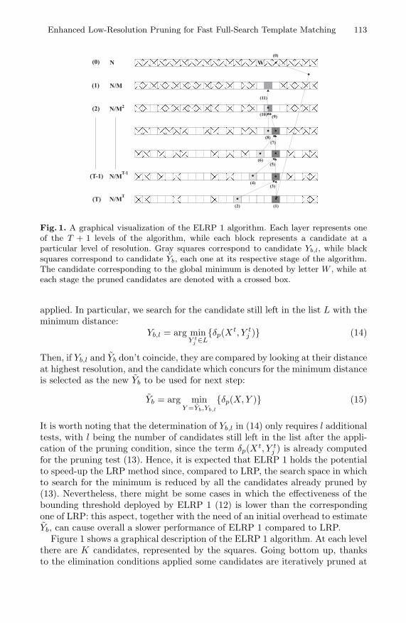
Fig. 1. A graphical visualization of the ELRP 1 algorithm. Each layer represents oneof the T + 1 levels of the algorithm, while each block represents a candidate at aparticular level of resolution. Gray squares correspond to candidate Yb,l, while blacksquares correspond to candidate Yb, each one at its respective stage of the algorithm.The candidate corresponding to the global minimum is denoted by letter W , while ateach stage the pruned candidates are denoted with a crossed box.

applied. In particular, we search for the candidate still left in the list L with theminimum distance:

Yb,l = arg minY t

j ∈L{δp(Xt, Y t

j )} (14)

Then, if Yb,l and Yb don’t coincide, they are compared by looking at their distanceat highest resolution, and the candidate which concurs for the minimum distanceis selected as the new Yb to be used for next step:

Yb = arg minY =Yb,Yb,l

{δp(X, Y )} (15)

It is worth noting that the determination of Yb,l in (14) only requires l additionaltests, with l being the number of candidates still left in the list after the appli-cation of the pruning condition, since the term δp(Xt, Y t

j ) is already computedfor the pruning test (13). Hence, it is expected that ELRP 1 holds the potentialto speed-up the LRP method since, compared to LRP, the search space in whichto search for the minimum is reduced by all the candidates already pruned by(13). Nevertheless, there might be some cases in which the effectiveness of thebounding threshold deployed by ELRP 1 (12) is lower than the correspondingone of LRP: this aspect, together with the need of an initial overhead to estimateYb, can cause overall a slower performance of ELRP 1 compared to LRP.

Figure 1 shows a graphical description of the ELRP 1 algorithm. At each levelthere are K candidates, represented by the squares. Going bottom up, thanksto the elimination conditions applied some candidates are iteratively pruned at


each level (denoted by the crossed boxes), while the others are propagated up tothe top level, where the exhaustive search is determined on the left vectors andthe best candidate is found (denoted by W ). At start-up, i.e. step (0), candidateYb is determined by means of the non-exhaustive technique and used to prune thecandidates at level T. Then, at each level, after applying the pruning condition(13) on the candidates still in the list, the two vectors Yb and Yb,l (respectively,the black and the gray squares) are compared and the best between the two athighest level (i.e. 0) is chosen (15) as Yb for the upper level.

3.2 ELRP 2

As outlined in Section 2, at each step t the LRP algorithm performs an exhaustivesearch between the candidates left in the list in order to determine Yb as thecandidate which corresponds to the minimum distance, so that it can be usedfor the computation of the threshold Dt. Conversely, method ELRP 1 reducesthis search at each step by means of Yb and a strategy for updating Yb by means ofYb,l. A different approach is devised by keeping the exhaustive search performedbetween the candidates left at the lower level. With this approach, at each stept we first determine Yb as the candidate yielding the minimum score at level tbetween the candidates left in the list. Then, Yb is updated as:

Yb = arg minY =Yb,Yb

{δp(X, Y )} (16)

It is worth to note that also this approach contains a strategy which allowsfor using a different candidate in case Yb is estimated badly by the initial non-exhaustive step. This is performed by means of the comparison in (16). It isalso important to point out that, thanks to (16), the bounding terms deployedby ELRP 2 are guaranteed being always more (or, at worst, equally) effectivecompared than the corresponding ones devised by LRP. In terms of performance,this guarantees that in the worst case ELRP 2 will be slower than LRP onlyfor the amount of time needed to carry out the estimation of Yb, which, aspreviously mentioned, has to be small compared to the overall time required bythe algorithm.

3.3 ELRP 3

In this third approach, we propose to change the rule by which the candidatesare tested. Each candidate Yj is compared (13) against all the possible pruningconditions which can be determined until either it is pruned, or the last level(i.e. level 0) is reached, which means the distance between X and Yj must becomputed. Of course, the succession of the pruning conditions follows the originalalgorithm, going from the lowest level (i.e. level T ) up to the highest one. Hence,each candidate will be individually tested against up to T pruning conditions.

This approach allows to devise an updating procedure as follows. At the be-ginning of the algorithm, the thresholds Dt are computed at each level by means


of Yb. When a candidate Yj can not be skipped by any of the T conditions ap-plied, the actual distance δp(X, Yj) must be computed and the best candidate isupdated as:

Yb = arg minY =Yb,Yj

{δp(X, Y )} (17)

Furthermore, the algorithm does not need anymore to keep a list where to storethe candidates which have not been pruned so far, with extra savings for whatmeans operations and memory requirements.

4 Experimental Results

This section compares the results obtained using the ELRP 1, ELRP 2 and ELRP3 algorithms described in Section 3 with those yielded by the LRP algorithm.In the situation considered in [1], i.e. images affected by artificial noise, LRPyields notable speed-ups with respect to the FS algorithm. Nevertheless, we arealso interested in testing the algorithms with more typical distortions found inreal-world applications, i.e. those generated by slight changes in illumination andposition. Thus, we carry out two experiments.

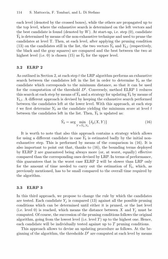
Fig. 2. The reference image used in Experiment 1 (top, left) and 2 (top, right). Bottom:the 10 templates used in the experiments are highlighted by black boxes.


In the first experiment 10 templates are extracted from an image as shown infig. 2 (bottom), then the reference image is chosen as an image taken at a differ-ent time instant from a close-by position and with slightly different illuminationconditions (see Figure 2, top left). Hence, the distortions between the templatesand the reference image are generated by slight changes in pose and illumina-tion, which can be regarded as the typical distortions found in real templatematching scenarios. Then, in order to complete the experimental framework, wepropose another experiment where the proposed algorithms are tested in thesame conditions as in [1], that is, artificial noise is added to the image wherethe templates where extracted from (see Figure 2, top right). In particular, theintroduced distortion is represented by i.i.d. double exponential (Laplace) dis-tributed noise with parameters σ = 10 and μ = 0. The 10 templates are thesame as in experiment 1 (Figure 2, bottom).

To be coherent with the experimental framework proposed in [1], each tem-plate used for the two experiments is of size 64 × 64. This allows to haveM = 4 = 2 × 2, and the number of pruning levels T = 6. For the same reason,we use here the SSD function (i.e. p = 2). All the algorithms deploy incremen-tal calculation techniques (i.e. [6]) for efficient computation of the transformedcandidates at each level of resolution. Finally, the benchmark platform was aLinux workstation based on a P4 3.056 GHz processor; the algorithms wereimplemented in C and compiled using Gcc with optimization level O3.

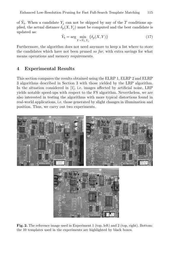
Table 1. Measured speed-ups against FS in Experiment 1

Template LRP ELRP1ELRP2ELRP3T1 11.3 17.9 16.4 17.9T2 26.0 43.8 35.8 47.9T3 7.1 9.9 9.5 9.8T4 5.0 9.9 9.7 9.8T5 18.2 28.6 25.2 29.8T6 11.4 25.5 22.8 26.4T7 13.1 25.0 22.2 25.7T8 22.1 27.7 24.4 28.9T9 11.5 12.8 ∗ 14.2 ∗ 24.0 ∗T10 11.6 11.0 ∗ 11.5 ∗ 17.2 ∗

Mean 13.7 21.2 19.2 23.7St.Dev. 6.5 11.0 8.4 11.2

Table 1 and Table 2 show the speed-ups (i.e. ratios of measured executiontimes) yielded by LRP, ELRP 1, ELRP 2 and ELRP 3 with regards to theFS SSD-based algorithm. As for the ELRP algorithms, the execution times in-clude also the initial non-exhaustive step. Table 1 is relative to the dataset ofexperiment 1, while Table 2 shows the results concerning experiment 2. Fur-thermore, in the two tables symbol ∗ is used to highlight those cases where thenon-exhaustive algorithm applied at the first step does not find the global min-imum: overall, this happens in 3 cases out of 20. Nevertheless, though already


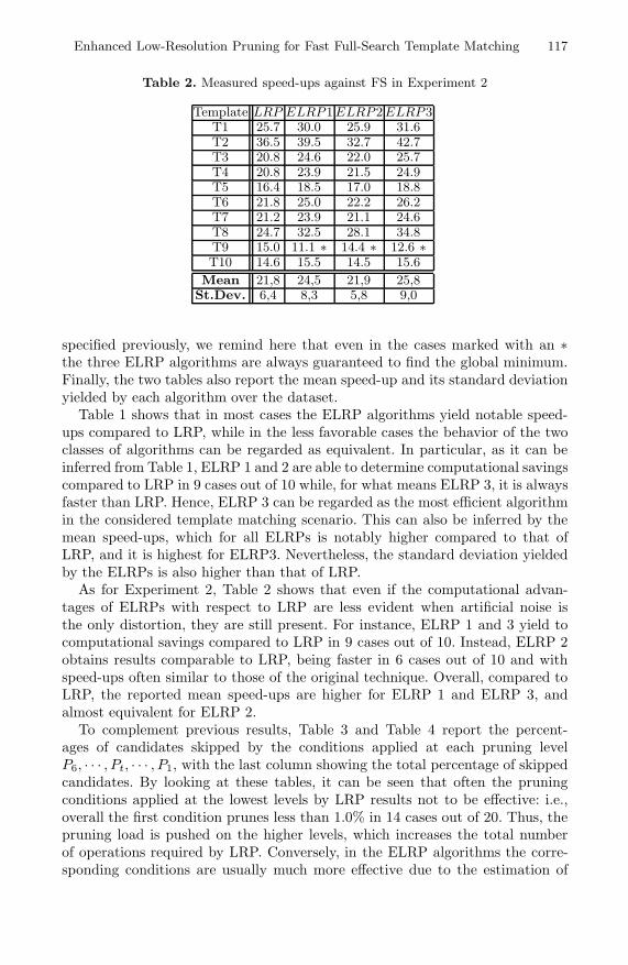
Table 2. Measured speed-ups against FS in Experiment 2

Template LRP ELRP1ELRP2ELRP3T1 25.7 30.0 25.9 31.6T2 36.5 39.5 32.7 42.7T3 20.8 24.6 22.0 25.7T4 20.8 23.9 21.5 24.9T5 16.4 18.5 17.0 18.8T6 21.8 25.0 22.2 26.2T7 21.2 23.9 21.1 24.6T8 24.7 32.5 28.1 34.8T9 15.0 11.1 ∗ 14.4 ∗ 12.6 ∗T10 14.6 15.5 14.5 15.6

Mean 21,8 24,5 21,9 25,8St.Dev. 6,4 8,3 5,8 9,0

specified previously, we remind here that even in the cases marked with an ∗the three ELRP algorithms are always guaranteed to find the global minimum.Finally, the two tables also report the mean speed-up and its standard deviationyielded by each algorithm over the dataset.

Table 1 shows that in most cases the ELRP algorithms yield notable speed-ups compared to LRP, while in the less favorable cases the behavior of the twoclasses of algorithms can be regarded as equivalent. In particular, as it can beinferred from Table 1, ELRP 1 and 2 are able to determine computational savingscompared to LRP in 9 cases out of 10 while, for what means ELRP 3, it is alwaysfaster than LRP. Hence, ELRP 3 can be regarded as the most efficient algorithmin the considered template matching scenario. This can also be inferred by themean speed-ups, which for all ELRPs is notably higher compared to that ofLRP, and it is highest for ELRP3. Nevertheless, the standard deviation yieldedby the ELRPs is also higher than that of LRP.

As for Experiment 2, Table 2 shows that even if the computational advan-tages of ELRPs with respect to LRP are less evident when artificial noise isthe only distortion, they are still present. For instance, ELRP 1 and 3 yield tocomputational savings compared to LRP in 9 cases out of 10. Instead, ELRP 2obtains results comparable to LRP, being faster in 6 cases out of 10 and withspeed-ups often similar to those of the original technique. Overall, compared toLRP, the reported mean speed-ups are higher for ELRP 1 and ELRP 3, andalmost equivalent for ELRP 2.

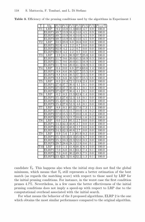
To complement previous results, Table 3 and Table 4 report the percent-ages of candidates skipped by the conditions applied at each pruning levelP6, · · · , Pt, · · · , P1, with the last column showing the total percentage of skippedcandidates. By looking at these tables, it can be seen that often the pruningconditions applied at the lowest levels by LRP results not to be effective: i.e.,overall the first condition prunes less than 1.0% in 14 cases out of 20. Thus, thepruning load is pushed on the higher levels, which increases the total numberof operations required by LRP. Conversely, in the ELRP algorithms the corre-sponding conditions are usually much more effective due to the estimation of


Table 3. Efficiency of the pruning conditions used by the algorithms in Experiment 1

T Alg P6% P5% P4% P3% P2% P1% PTOT %T1 LRP 9.2 13.8 11.3 60.0 4.7 0.9 100.0

ELRP1 49.7 13.9 16.4 14.6 4.5 0.9 100.0ELRP2 49.7 13.9 16.4 14.6 4.5 0.9 100.0ELRP3 49.7 13.9 16.4 14.6 4.5 0.9 100.0

T2 LRP 53.5 23.8 6.0 16.6 0.0 0.0 100.0ELRP1 92.9 4.2 2.2 0.7 0.0 0.0 100.0ELRP2 92.9 4.2 2.2 0.7 0.0 0.0 100.0ELRP3 92.9 4.2 2.2 0.7 0.0 0.0 100.0









candidate Yb. This happens also when the initial step does not find the globalminimum, which means that Yb still represents a better estimation of the bestmatch (as regards the matching score) with respect to those used by LRP forthe initial pruning conditions. For instance, in the worst case the first conditionprunes 4.7%. Nevertheless, in a few cases the better effectiveness of the initialpruning conditions does not imply a speed-up with respect to LRP due to thecomputational overhead associated with the initial search.

For what means the behavior of the 3 proposed algorithms, ELRP 2 is the onewhich obtains the most similar performance compared to the original algorithm.


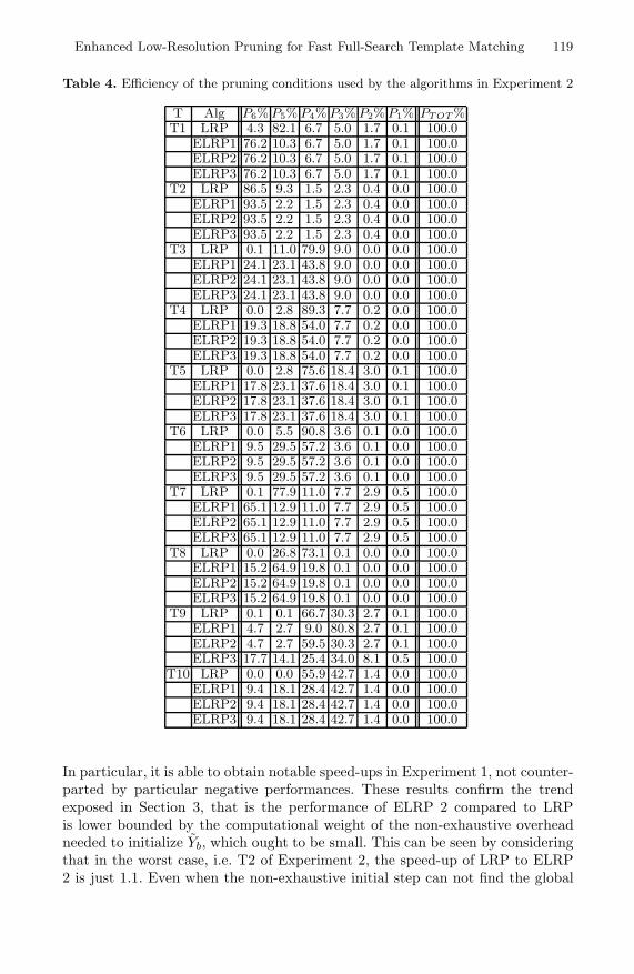
Table 4. Efficiency of the pruning conditions used by the algorithms in Experiment 2

T Alg P6% P5% P4% P3% P2% P1% PTOT %T1 LRP 4.3 82.1 6.7 5.0 1.7 0.1 100.0

ELRP1 76.2 10.3 6.7 5.0 1.7 0.1 100.0ELRP2 76.2 10.3 6.7 5.0 1.7 0.1 100.0ELRP3 76.2 10.3 6.7 5.0 1.7 0.1 100.0










In particular, it is able to obtain notable speed-ups in Experiment 1, not counter-parted by particular negative performances. These results confirm the trendexposed in Section 3, that is the performance of ELRP 2 compared to LRPis lower bounded by the computational weight of the non-exhaustive overheadneeded to initialize Yb, which ought to be small. This can be seen by consideringthat in the worst case, i.e. T2 of Experiment 2, the speed-up of LRP to ELRP2 is just 1.1. Even when the non-exhaustive initial step can not find the global


minimum (i.e. the ∗-cases in the tables) the behavior of the algorithm turns outto be at worst very close to that of LRP. In addition, it is also interesting tonote that tables 3, 4 confirm that the aggregated candidates pruned by ELRP2 at each conditions are always equal or higher than those pruned respectivelyby the conditions devised by LRP.

On the other hand, experimental results demonstrate that the strategies de-ployed by ELRP 1 and ELRP 3 are more effective than that of LRP since theyboth are able to obtain higher benefits in terms of computational savings com-pared to ELRP 2 on the average. In particular, ELRP 3 is the algorithm whichyields the highest speed-ups and whose behavior is always favorable compared toLRP along the considered dataset, with the exception of a single instance wherethe speed-up obtained by ELRP 3 is slightly less than that of LRP. Hence, it canbe regarded as the best algorithm, especially if the distortions between imageand template are those typically found in real template matching applications.

5 Conclusions

We have shown how the LRP technique described in [1] can be enhanced bymeans of three different full-search equivalent algorithms (referred to as ELRP1, ELRP 2 and ELRP 3), which deploy an initial estimation of a good candidateto be used in the pruning process. The proposed algorithms are able to yieldsignificant speed-ups compared to the LRP technique in an experimental frame-work where distortions between templates and reference images are representedby changes in pose and illumination as well as by artificial noise. The variationsproposed in our work do not increase the memory requirements of the originalalgorithm. Besides, it comes natural to expect that further improvements can beobtained if a more efficient non-exhaustive technique is used to determine theinitial candidate, Yb, in spite of the naive method we implemented for our tests.

References

1. Gharavi-Alkhansari, M.: A fast globally optimal algorithm for template matchingusing low-resolution pruning. IEEE Trans. Image Processing 10(4), 526–533 (2001)

2. Goshtasby, A.: 2-D and 3-D image registration for medical, remote sensing andindustrial applications. Wiley, Chichester (2005)

3. Barnea, D., Silverman, H.: A class of algorithms for digital image registration. IEEETrans. on Computers C-21(2), 179–186 (1972)

4. Li, W., Salari, E.: Successive elimination algorithm for motion estimation. IEEETrans. on Image Processing 4(1), 105–107 (1995)

5. Wang, H., Mersereau, R.: Fast algorithms for the estimation of motion vectors. IEEETrans. on Image Processing 8(3), 435–439 (1999)

6. Mc Donnel, M.: Box-filtering techniques. Computer Graphics and Image Process-ing 17, 65–70 (1981)

Documents

Enhanced Low-Resolution Pruning for Fast Full-Search ...vision.deis.unibo.it/fede/papers/acivs09-2.pdf · Enhanced Low-Resolution Pruning for Fast Full-Search Template Matching 111