Embed Size (px)
Citation preview
i
The Islamic University of Gaza
Deanery of Graduate Studies
Faculty of Engineering
Computer Engineering Department
Enhanced k-means Clustering
Algorithm
by
Abdessalam H. Elhabbash
Supervisor: Prof. Hatem Hamad
A Thesis Submitted in Partial Fulfillment of the Requirements for the
Degree of Master in Computer Engineering
0212 -هـ 1341

ii
Abstract
Data clustering is an unsupervised classification method aims at creating groups of
objects, or clusters, in such a way that objects in the same cluster are very similar and
objects in different clusters are quite distinct. Though k-means is very popular for general
clustering, it suffers from some disadvantages such as (1) Its performance depends highly
on initial cluster centers, (2) The number of clusters must be previously known and fixed,
and (3) The algorithm contains the dead-unit problem which results in empty clusters.
Random k-means initialization generally leads k-means to converge to local minima i.e.
inacceptable clustering results are produced. In this thesis a method based on some rough
set theory concepts and reverse nearest neighbor search is proposed to find the appropriate
initial centers for the k-means clustering problem. The complexity of the proposed method
is analyzed as well. Also, a method is described to determine the number of clusters in a
dataset. Experimental results show the accuracy and effectiveness of the proposed methods.
Keywords: data clustering, k-means, initialization, cohesion degree, RNN

iii
k-means
k-meansrough
set theorycohesion degree RNN degree
k-means
iv
Dedication
To whom I love

v
Acknowledgment
My thanks to all those who generously contributed
their favorite recipes. Without their help, this work
would have never been possible.
vi
Table of Contents
1 Introduction 1
1.1 Clustering Vocabularies 4
1.2.1 Datasets 5
1.2.2 Objects and Attributes 5
1.2.3 Data Types 5
1.2.4 Similarity and Dissimilarity 6
1.2.5 Clusters and Cluster Center 7
1.2.6 Hard Clustering and Fuzzy Clustering 7
1.2 Background 9
1.3 Problem Statement 12
2 Related Work 16
3 Enhanced k-means 27
6.1 Some Basic Definitions 27
3.1.1 Cohesion degree 27
3.1.2 Coupling degree 29
3.1.3 Reverse Nearest Neighbor 29
3.1.4 Example 30
6.2 An initialization method for the K-Means algorithm using
neighborhood model 34
6.3 Proposed enhancements 35
A. Fast k-means Initialization method using Neighborhood and
Reverse Nearest Neighborhood models 36
vii
B. Auto-determining the number of clusters using Neighborhood and
Reverse Nearest Neighborhood models 38
4 Experimental Results 42
4.1 Results of Initialization algorithms 42
4.2 Results of Auto-determining k 45
5 Conclusion and Future Research 48
References 49
viii
List of Tables
Table 3.1 Example Dataset 31
Table 3.2 Distances between the Objects in Figure 3.2 33
Table 4.1 Results of experiments on Iris dataset 44
Table 4.2 Results of experiments on Wine dataset 44
Table 4.3 Results of experiments on Glass dataset 44
Table 4.4 Results of experiments on Test dataset 44
Table 4.5 k Determination Results 47
ix
List of Figures
Figure 1.1 Three well-separated clusters 8
Figure 1.2 k-means clustering example 10
Figure 1.3 Clustering problem example in k-means 12
Figure 1.4 Dead point Problem 15
Figure 2.1 Neighborhood Model Algorithm 20
Figure 2.2 CCIA Algorithm 23
Figure 2.3 IRNN Algorithm 24
Figure 2.4 kd-tree Initialization Algorithm 27
Figure 2.5 k'-means Algorithm 28
Figure 3.1 RNN definition 32
Figure 3.2 Example dataset 33
Figure 3.3 High RC objects 41
Figure 4.1 Test dataset 45
x
List of Abbreviations
AC Accuracy
AGNES AGglomerative NESting
BIRCH Balanced Iterative Reducing and Clustering using Hierarchies
CCIA Cluster Center Initialization Algorithm
CLIQUE CLustering InQUEst
CS Candidate Set
DBSCAN Density-Based Spatial Clustering of Applications with Noise
DIANA DIvisiveANAlysis
IRNN Initialization by Reverse Nearest Neighbor
NN Nearest Neighbor
OPTICS Ordering Points to Identify the Clustering Structure
pCluster Clustering by pattern similarity in large data sets
PROCLUS PROjected CLUSting
RFN Reverse Farthest Neighbor
RNN Reverse Nearest Neighbor
STING STatistical INformation Grid-based clustering
1
Chapter 1:Introduction
Machine learning is a subfield of artificial intelligence that is concerned with the
design, analysis, implementation, and applications of programs that learn from experience.
Machine learning is classified as supervised learning or unsupervised learning. In the
former the set of training data is available, and a classification algorithm is designed by
exploiting this a priori known information to classify the data points into pre-defined
classes. In the latter, there is no a priori knowledge about the classes of the data points [1].
Data clustering (or just clustering), is an unsupervised classification method aims at
creating groups of objects, or clusters, in such a way that objects in the same cluster are
very similar and objects in different clusters are quite distinct [2].
Cluster analysis has been widely used in numerous applications, including market
research, pattern recognition, data analysis, and image processing. In business, clustering
can help marketers discover interests of their customers based on purchasing patterns and
characterize groups of the customers. In biology, it can be used to derive plant and animal
taxonomies, categorize genes with similar functionality, and gain insight into structures
inherent in populations. In geology, specialist can employ clustering to identify areas of
similar lands, similar houses in a city and etc. data clustering can also be helpful in
classifying documents on the Web for information discovery [3].
Data clustering, also called cluster analysis, is a challenging field of research in which
applications pose their own special requirements. Data mining applications place the
following special requirements on clustering techniques [3]:
2
- Scalability: Clustering applications may have a large database that contains millions
of objects. So, highly scalable clustering algorithms are needed to successfully form the
clusters.
- Ability to deal with different types of attributes: data points may have different
types such as numerical, ordinal, categorical, and binary [2]. Different applications may
require clustering data of a one type of mixture of data types.
- Arbitrary shape discovery: Some clustering algorithms determine clusters based on
distance measurement such as Euclidean. These algorithms form spherical clusters. Other
clustering algorithms are needed to find clusters of arbitrary shapes such as those based on
density.
- Insensitivity to noise: Clustering algorithms are needed to be insensitive to noise
and outlier data to avoid the result of poor clustering.
- High dimensionality: Many clustering algorithms can efficiently find clusters of low
dimensional data. However, clustering in high dimensional space is a challenging task since
distances between objects become very large and average density of points is likely to be
quite low.
In the literature, many clustering algorithms have been proposed. These algorithms differ
from each other by the criteria considered which lead to different categories of clustering
algorithms. Although it is difficult to find strict categorization of the clustering algorithms
because the categories may overlap, the following categorization is helpful to discriminate
the clustering algorithms [3]:
3
Partitioning methods: A partitioning method creates k partitions (or clusters) such
that k ≤ n where n is the total number of objects. It creates an initial portioning and then
iteratively moves the objects from one cluster to another to improve the partitioning. Good
clustering is that the similarity between objects in the same cluster is high whereas the
dissimilarity between objects in the different clusters is high. The k-means algorithm is a
commonly used partitioning method [4].
Hierarchical methods: A hierarchical method creates a hierarchal structure of the
data objects. Then a given number k of clusters determines how to cut the hierarchy. It can
be either agglomerative or divisive. The agglomerative approach starts by considering each
object as a separate cluster. Then it iteratively merges the most similar clusters until
grouping all the objects in one cluster. The divisive approach starts by considering the
entire objects as one cluster. Then it iteratively splits each cluster into smaller clusters until
each objects forms its own cluster. AGNES and DIANA [5] are examples of hierarchical
clustering. BIRCH [6] integrates hierarchical clustering with iterative (distance-based)
relocation.
Density-based methods: The idea behind these methods is to group dense objects
into clusters. An object is dense if its neighborhood if a given clusters contains at least
minimum number of objects. These methods have the advantage to find clusters with
arbitrary shapes and they are insensitive to noise and outliers. DBSCAN [7] and OPTICS
[8] are typical examples of density-based clustering.
Grid-based methods: These methods divide the object space into a finite number of
cells that form a grid structure. Therewith connected cells are grouped in a cluster. STING
4
[9] is an example of grid-based clustering. Some techniques such as CLIQUE [10] combine
both density-based and grid-based approaches. The main advantages of these methods are
fast processing and arbitrary-shape clusters foundation.
Model-based methods: This approach creates a mathematical model for each of the
clusters and finds the best fit of the data to the given model. A main advantage is that these
methods automatically determine the number of clusters based on standard statistics.
COBWEB [11] and self-organizing feature maps [12] are examples of model-based
clustering.
Methods for high-dimensional data: Distance- and Density-based methods are
inefficient for clustering high-dimensional data since objects are increasingly sparse.
Alternative approaches, such as subspace clustering methods and frequent pattern-based
clustering, have been proposed. Subspace clustering methods search for clusters in
subspaces of the data, rather than over the entire data space. CLIQUE [10] and PROCLUS
[13] are examples of subspace clustering methods. Frequent pattern-based clustering
methods extract distinct frequent patterns among subsets of dimensions that occur
frequently. pCluster [25] is an example of frequent pattern-based clustering that groups
objects based on their pattern similarity.
1.1 Clustering Vocabularies
In this section, we introduce some basic concepts that are frequently encountered in the
field of cluster analysis, i.e. objects and attributes, similarity and dissimilarity, dataset, and
cluster centers.
5
1.1.1 Dataset
A dataset is a collection of data items that have different characteristics. In clustering,
these data items are grouped into clusters.
1.1.2 Objects and Attributes
An object is a single data item, i.e. a member in a dataset. It can also be referred to as
data point, pattern case, observation, individual, item, tuple, record, or object. An attribute
is value that specifies of a property of the object such as length, weight, etc. It can also be
referred to as variable, or feature.
Mathematically, a data set D with n objects, each of which is described by d attributes,
is denoted by , where is a vector denoting the
ith
object and is a scalar denoting the jth
component or attribute of . The number of
attributes d is also called the dimensionality of the data set [2].
1.1.3 Data Types
Data clustering algorithms are associated with types of data the attributes have [2]. An
attribute can be Binary, Categorical, Ordinal, Interval-scaled, or Ratio-Scaled [3].
- Binary attributes has only two states: 0 or 1, where 0 means that the variable is absent,
and 1 means that it is present.
- Categorical attributes, also referred to as nominal, are simply used as names, such as
the brands of cars and names of bank branches. That is, a categorical attribute is a
generalization of the binary variable; it can take on more than two states.
6
- Ordinal attributes resembles a categorical variable, except that the M states of the
ordinal value are ordered in a meaningful sequence. For example, professional ranks are
often enumerated in a sequential order, such as assistant, associate, and full for
professors.
- Interval-scaled attributes are continuous measurements of a linear scale such as
weight, height and weather temperature.
- Ratio-Scaled attributes make a positive measurement on a nonlinear scale. For
example an exponential scale, , and the volume of sales over time are ration-scaled
attributes.
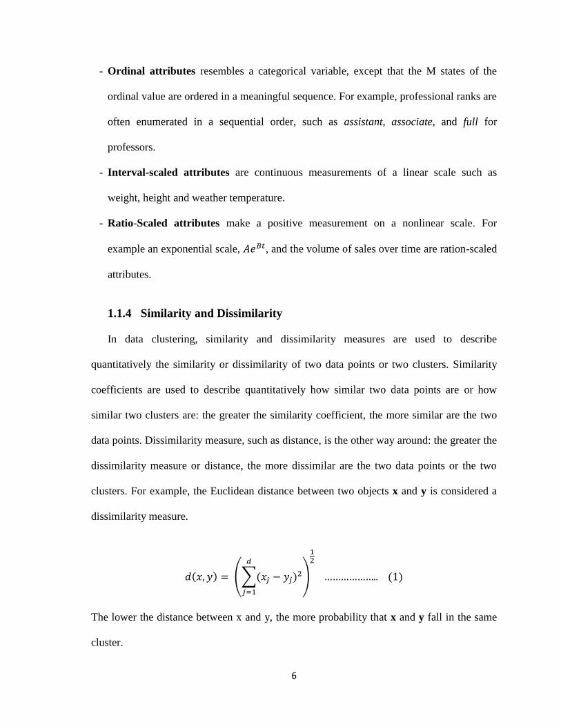
1.1.4 Similarity and Dissimilarity
In data clustering, similarity and dissimilarity measures are used to describe
quantitatively the similarity or dissimilarity of two data points or two clusters. Similarity
coefficients are used to describe quantitatively how similar two data points are or how
similar two clusters are: the greater the similarity coefficient, the more similar are the two
data points. Dissimilarity measure, such as distance, is the other way around: the greater the
dissimilarity measure or distance, the more dissimilar are the two data points or the two
clusters. For example, the Euclidean distance between two objects x and y is considered a
dissimilarity measure.
(∑
)
The lower the distance between x and y, the more probability that x and y fall in the same
cluster.
7
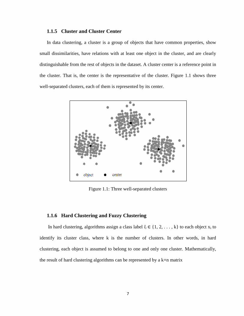
1.1.5 Cluster and Cluster Center
In data clustering, a cluster is a group of objects that have common properties, show
small dissimilarities, have relations with at least one object in the cluster, and are clearly
distinguishable from the rest of objects in the dataset. A cluster center is a reference point in
the cluster. That is, the center is the representative of the cluster. Figure 1.1 shows three
well-separated clusters, each of them is represented by its center.
Figure 1.1: Three well-separated clusters
1.1.6 Hard Clustering and Fuzzy Clustering
In hard clustering, algorithms assign a class label li {1, 2, . . . , k} to each object xi to
identify its cluster class, where k is the number of clusters. In other words, in hard
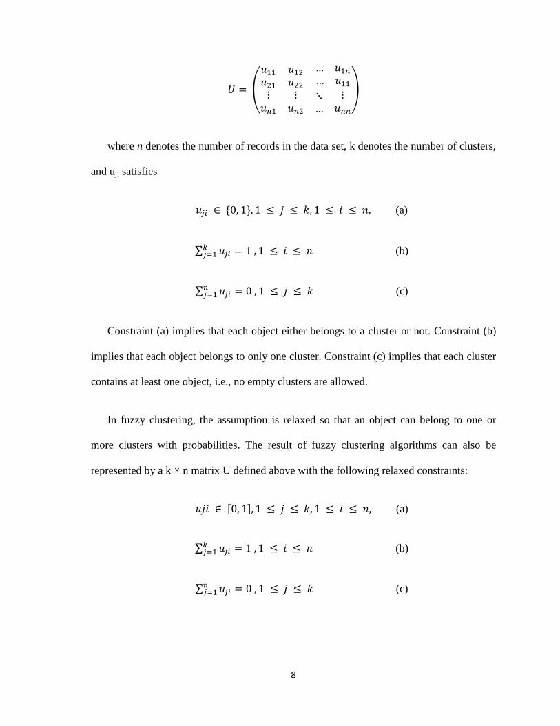
clustering, each object is assumed to belong to one and only one cluster. Mathematically,
the result of hard clustering algorithms can be represented by a k×n matrix
8
(
)
where n denotes the number of records in the data set, k denotes the number of clusters,
and uji satisfies
(a)
∑ (b)
∑ (c)
Constraint (a) implies that each object either belongs to a cluster or not. Constraint (b)
implies that each object belongs to only one cluster. Constraint (c) implies that each cluster
contains at least one object, i.e., no empty clusters are allowed.
In fuzzy clustering, the assumption is relaxed so that an object can belong to one or
more clusters with probabilities. The result of fuzzy clustering algorithms can also be
represented by a k × n matrix U defined above with the following relaxed constraints:
[ ] (a)
∑ (b)
∑ (c)
9
1.2 Background
The k-means algorithm is the choice for many clustering tasks, especially with low
dimension datasets. This algorithm is a partitional one. It takes the input parameter k, the
number of clusters, and partitions a set of n objects into k clusters so that the resulting intra-
cluster similarity is high but the inter-cluster similarity is low. The algorithm attempts to
find the cluster centers, (C1 …… Ck), such that the sum of the squared distances of each
data point, xi , 1 ≤ i ≤ n ,to its nearest cluster center Cj, 1 ≤ j ≤ k, is minimized. First, the
algorithm randomly selects the k objects, each of which initially represents a cluster mean
or center. Then, each object xi in the data set is assigned to the nearest cluster center .i.e to
the most similar center. The algorithm then computes the new mean for each cluster and
reassigns each object to the nearest new center. This process iterates until no changes occur
to the assignment of objects. The convergence results in minimizing the sum-of-squares
error that is defined as the summation of the squared distances from each object to its
cluster center as in formula (2) [4, 30].
∑ ∑
where SSE is the sum-of-squares error for all objects in the data set; xi is an object; and mj
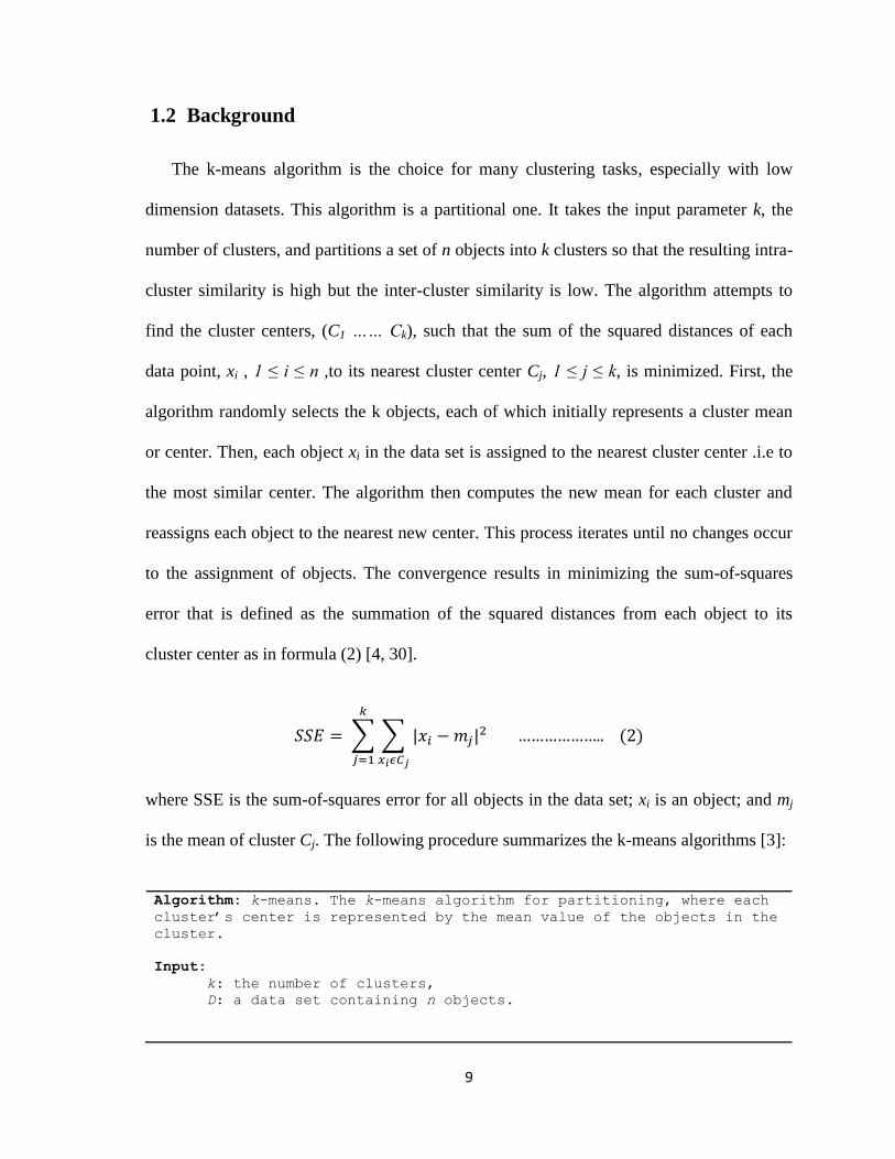
is the mean of cluster Cj. The following procedure summarizes the k-means algorithms [3]:
Algorithm: k-means. The k-means algorithm for partitioning, where each
cluster’s center is represented by the mean value of the objects in the
cluster.
Input:
k: the number of clusters,
D: a data set containing n objects.
10
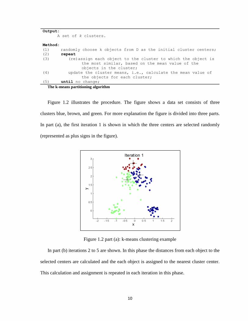
Output:
A set of k clusters.
Method:
(1) randomly choose k objects from D as the initial cluster centers;
(2) repeat
(3) (re)assign each object to the cluster to which the object is
the most similar, based on the mean value of the
objects in the cluster;
(4) update the cluster means, i.e., calculate the mean value of
the objects for each cluster;
(5) until no change;
The k-means partitioning algorithm
Figure 1.2 illustrates the procedure. The figure shows a data set consists of three
clusters blue, brown, and green. For more explanation the figure is divided into three parts.
In part (a), the first iteration 1 is shown in which the three centers are selected randomly
(represented as plus signs in the figure).
Figure 1.2 part (a): k-means clustering example
In part (b) iterations 2 to 5 are shown. In this phase the distances from each object to the
selected centers are calculated and the each object is assigned to the nearest cluster center.
This calculation and assignment is repeated in each iteration in this phase.
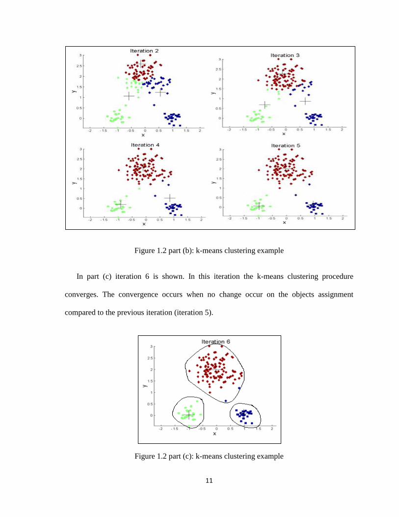
11
Figure 1.2 part (b): k-means clustering example
In part (c) iteration 6 is shown. In this iteration the k-means clustering procedure
converges. The convergence occurs when no change occur on the objects assignment
compared to the previous iteration (iteration 5).
Figure 1.2 part (c): k-means clustering example
12
1.3 Problem Statement
Despite being used in a wide array of applications, the k-means algorithm is not exempt
of drawbacks, mainly [19, 28]:
- As many clustering methods, the k-means algorithm assumes that the number of
clusters k in the database is known beforehand which, obviously, is not necessarily true
in real-world applications.
- As an iterative technique, the k-means algorithm is especially sensitive to initial centers
selection.
- The k-means algorithm may converge to local minima.
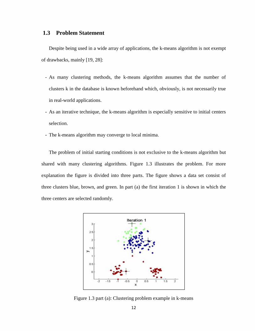
The problem of initial starting conditions is not exclusive to the k-means algorithm but
shared with many clustering algorithms. Figure 1.3 illustrates the problem. For more
explanation the figure is divided into three parts. The figure shows a data set consist of
three clusters blue, brown, and green. In part (a) the first iteration 1 is shown in which the
three centers are selected randomly.
Figure 1.3 part (a): Clustering problem example in k-means
13
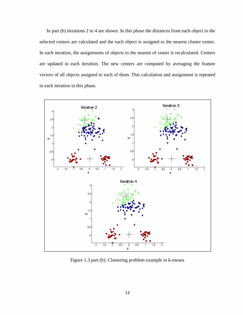
In part (b) iterations 2 to 4 are shown. In this phase the distances from each object to the
selected centers are calculated and the each object is assigned to the nearest cluster center.
In each iteration, the assignments of objects to the nearest of center is recalculated. Centers
are updated in each iteration. The new centers are computed by averaging the feature
vectors of all objects assigned to each of them. This calculation and assignment is repeated
in each iteration in this phase.
Figure 1.3 part (b): Clustering problem example in k-means
14
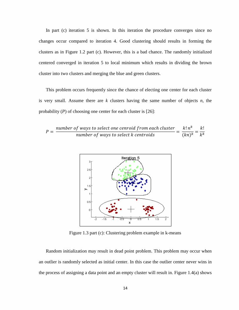
In part (c) iteration 5 is shown. In this iteration the procedure converges since no
changes occur compared to iteration 4. Good clustering should results in forming the
clusters as in Figure 1.2 part (c). However, this is a bad chance. The randomly initialized
centered converged in iteration 5 to local minimum which results in dividing the brown
cluster into two clusters and merging the blue and green clusters.
This problem occurs frequently since the chance of electing one center for each cluster
is very small. Assume there are k clusters having the same number of objects n, the
probability (P) of choosing one center for each cluster is [26]:
Figure 1.3 part (c): Clustering problem example in k-means
Random initialization may result in dead point problem. This problem may occur when
an outlier is randomly selected as initial center. In this case the outlier center never wins in
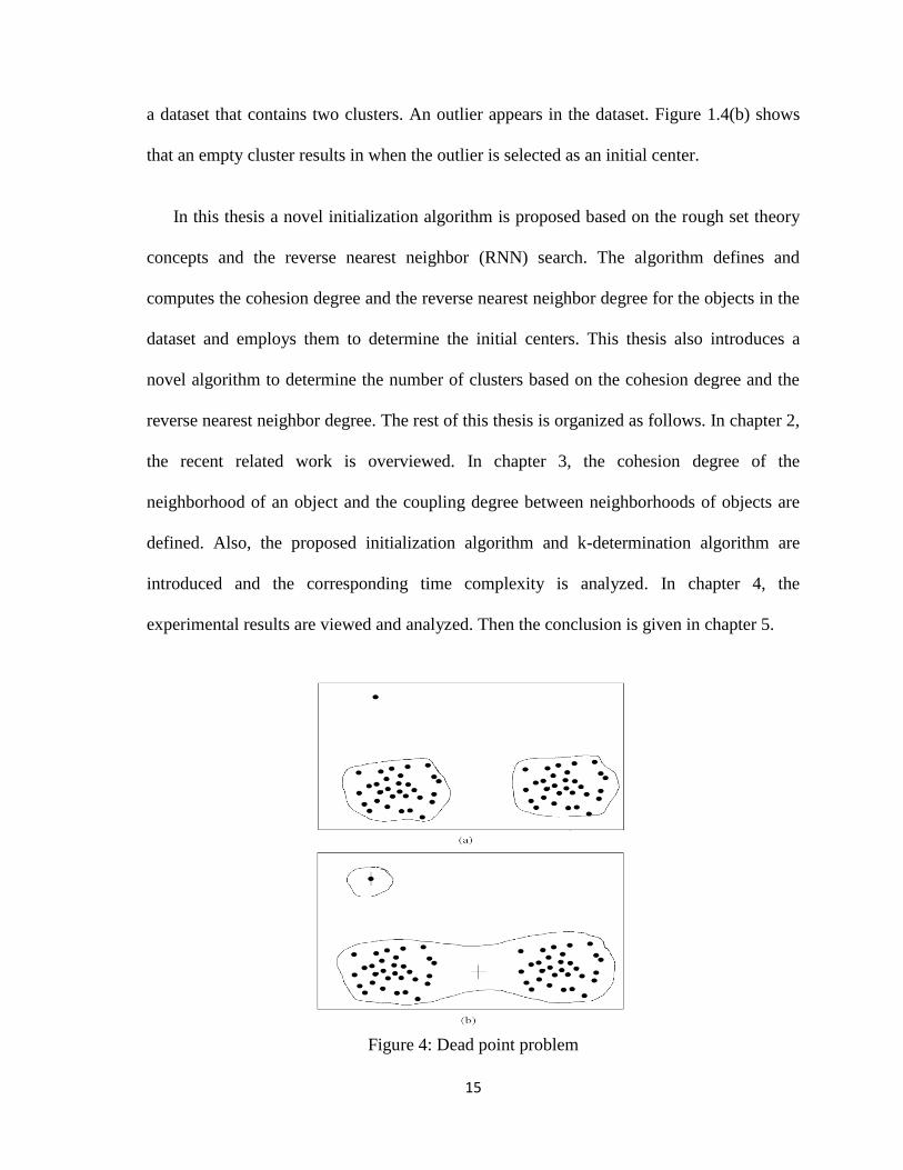
the process of assigning a data point and an empty cluster will result in. Figure 1.4(a) shows
15
a dataset that contains two clusters. An outlier appears in the dataset. Figure 1.4(b) shows
that an empty cluster results in when the outlier is selected as an initial center.
In this thesis a novel initialization algorithm is proposed based on the rough set theory
concepts and the reverse nearest neighbor (RNN) search. The algorithm defines and
computes the cohesion degree and the reverse nearest neighbor degree for the objects in the
dataset and employs them to determine the initial centers. This thesis also introduces a
novel algorithm to determine the number of clusters based on the cohesion degree and the
reverse nearest neighbor degree. The rest of this thesis is organized as follows. In chapter 2,
the recent related work is overviewed. In chapter 3, the cohesion degree of the
neighborhood of an object and the coupling degree between neighborhoods of objects are
defined. Also, the proposed initialization algorithm and k-determination algorithm are
introduced and the corresponding time complexity is analyzed. In chapter 4, the
experimental results are viewed and analyzed. Then the conclusion is given in chapter 5.
Figure 4: Dead point problem
16
Chapter 2: Related Work
Fuyuan et.al. [20] have presented a method for initializing k-means. Based on Rough
set Concepts [21] and neighborhood of objects, the method defines the cohesion degree of
the neighborhood of an object and the coupling degree between neighborhoods of objects.
Then the highest cohesion degree object is selected as the first center. After that, the
coupling degree between the first center and the next highest degree object is computed and
compared; if the coupling degree is less than some , the next highest degree object is
selected as the new center. Then the steps are repeated till selecting k centers where k is the
predefined number of clusters. The experiments are conducted on a PC with an Intel
Pentium 4 processor (2.4 GHz) and 1G byte memory running the Windows XP SP3
operating system. The K-Means algorithms with the three different initialization methods
are coded in MATLAB 7.0 programming language. To evaluate the efficiency of clustering
algorithms, three evaluation index accuracy (AC), precision (PR), and recall (RE) are
employed in the following experiments. In order to define the three kinds of evaluation
indexes, the following quantities were defined:
k - the number of classes of the data, which is known,
ai - the number of objects that are correctly assigned to the class Ci ,(1≤ i ≤ k)
bi - the number of objects that are incorrectly assigned to the class Ci,
ci - the number of objects that should be in, but are not correctly assigned to the class Ci
The accuracy, precision and recall are defined as:
17
∑
∑ (
)
∑
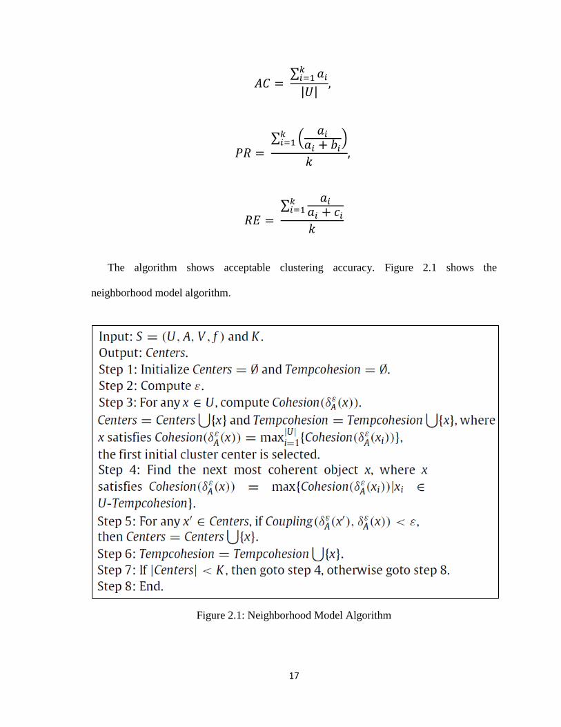
The algorithm shows acceptable clustering accuracy. Figure 2.1 shows the
neighborhood model algorithm.
Figure 2.1: Neighborhood Model Algorithm
18
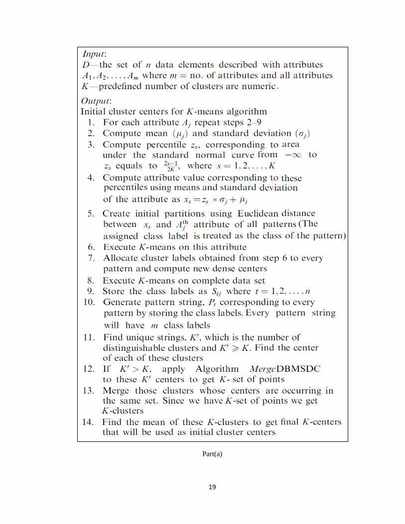
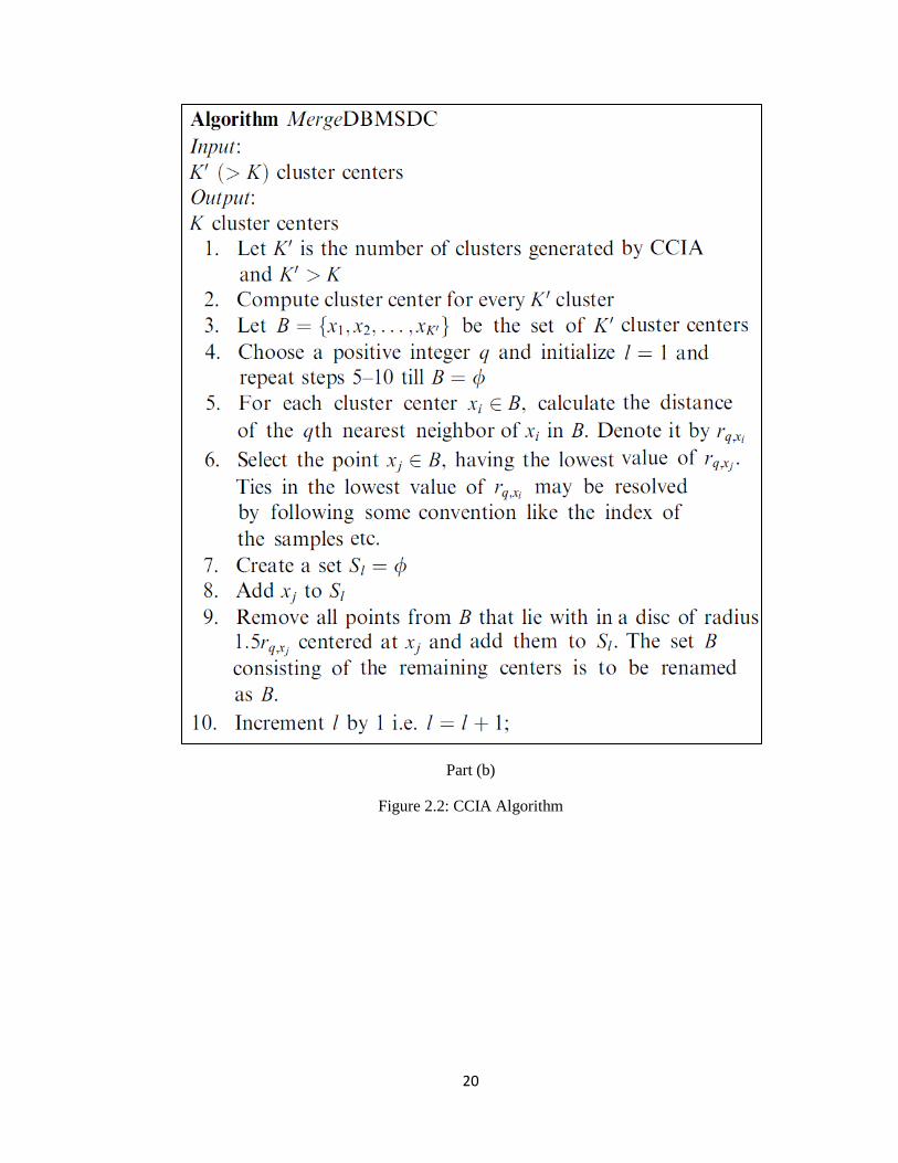
Khan and Ahmad [15] have presented an algorithm (CCIA) for computing initial cluster
centers for iterative clustering algorithm. CCIA procedure is based on the experimental fact
that very similar data points form the core of clusters and their cluster membership remain
the same. Hence these similar data points aid in finding initial cluster centers. Also, CCIA
depends on the observation that individual attribute provides information in computing
initial cluster centers. CCIA assumes that each of the attributes of the data points is
normally distributed. For k clusters the normal curve is divided into k partitions such that
the area under these partitions is equal. Then the midpoint of each interval is computed. The
attribute values corresponding to these midpoints are computed using mean and standard
deviation of the attribute. This will serve as seed point for the k-means clustering for this
attribute. This process generates a sequence of m cluster labels. The process is repeated for
all the attributes which generates k' sequences that correspond to k' clusters. If k' is equal to
k, then centers of these k' clusters should be treated as the initial cluster centers for the k-
means algorithm. If k' is greater than the number of desired clusters k, similar clusters are
merged to get k-clusters and centers of these k-clusters will become initial cluster centers
for the k-means algorithm. Figure 2.2 shows the CCIA algorithm.
19
Part(a)
20
Part (b)
Figure 2.2: CCIA Algorithm
21
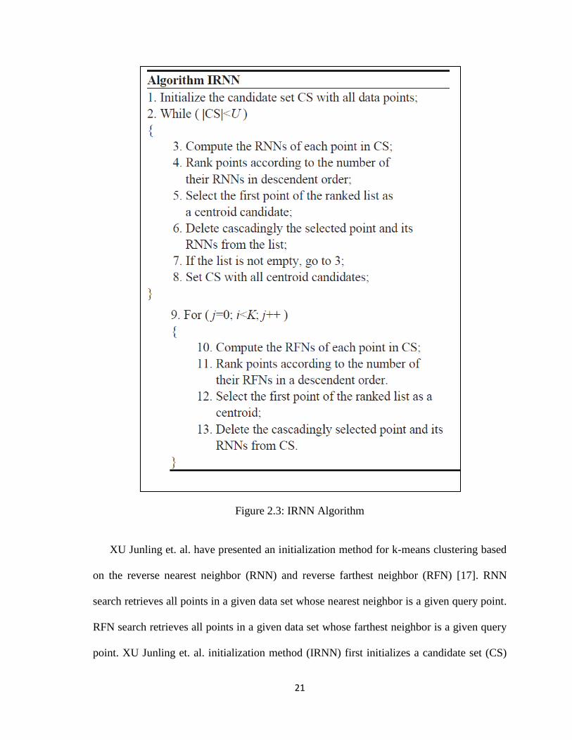
Figure 2.3: IRNN Algorithm
XU Junling et. al. have presented an initialization method for k-means clustering based
on the reverse nearest neighbor (RNN) and reverse farthest neighbor (RFN) [17]. RNN
search retrieves all points in a given data set whose nearest neighbor is a given query point.
RFN search retrieves all points in a given data set whose farthest neighbor is a given query
point. XU Junling et. al. initialization method (IRNN) first initializes a candidate set (CS)
22
with all data points, computes the RNNs of each point in CS, and ranks points according to
the number of their RNNs in a descending order; then it selects the first point of the ranked
list as a center candidate, and cascadingly deletes the selected point and its RNNs from the
list. If the list is not empty, the process of selection and deletion is repeated. After each
iteration, the method lets CS be the set of selected points and repeats the above process
until |CS| is less than some given number U. Finally, k centers are selected according to the
RFN criteria. Figure 2.3 shows the algorithm. The time complexity for the IRNN algorithm
is exponential since the process of selection and deletion is repeated many times and in
each iteration the RNN degrees, sorting, and deletion are repeated.
J.F. Lu et. al. proposed a hierarchical initialization approach for the k-means
initialization [14]. The proposed algorithm consists of four main procedures; they are
preprocessing, bottom–up procedure, top–down procedure and post processing. The
purpose of preprocessing is to transform the data into the form that is required by the
algorithm. The bottom–up and top–down procedure is the core of the algorithm, carrying
out both sampling and clustering. The post processing reverses the preprocessing operation
by inverse coordinate transformation to obtain the cluster centers in the original data. In the
sampling procedure the preprocessed data is sampled level by level by repetitively applying
a sampling method till the resampled data amount is the minimal number that is greater
than or equal to 20 * the number of clusters k. At the level that the sampling ends, iterative
clustering is executed so as to get the cluster centers. For the choice of initial centers, data
is sorted by weight value, and then the first k biggest instances are selected as the initial
cluster centers for the iteration.
23
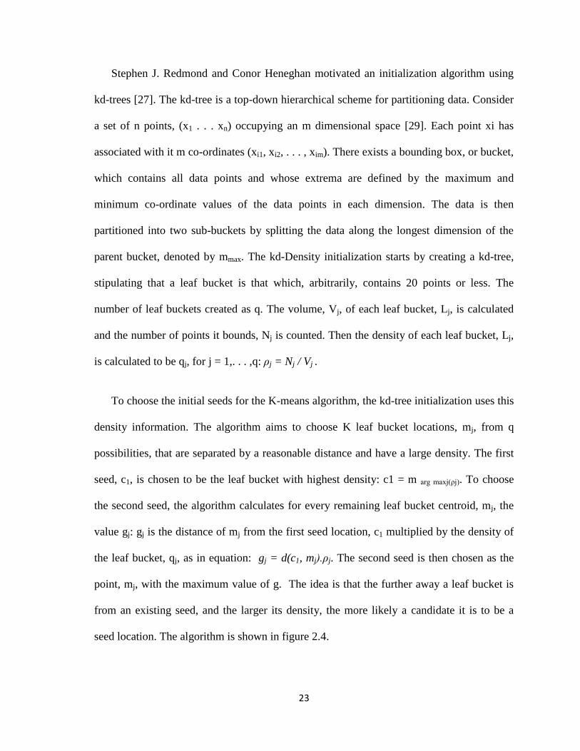
Stephen J. Redmond and Conor Heneghan motivated an initialization algorithm using
kd-trees [27]. The kd-tree is a top-down hierarchical scheme for partitioning data. Consider
a set of n points, (x1 . . . xn) occupying an m dimensional space [29]. Each point xi has
associated with it m co-ordinates (xi1, xi2, . . . , xim). There exists a bounding box, or bucket,
which contains all data points and whose extrema are defined by the maximum and
minimum co-ordinate values of the data points in each dimension. The data is then
partitioned into two sub-buckets by splitting the data along the longest dimension of the
parent bucket, denoted by mmax. The kd-Density initialization starts by creating a kd-tree,
stipulating that a leaf bucket is that which, arbitrarily, contains 20 points or less. The
number of leaf buckets created as q. The volume, Vj, of each leaf bucket, Lj, is calculated
and the number of points it bounds, Nj is counted. Then the density of each leaf bucket, Lj,
is calculated to be qj, for j = 1,. . . ,q: ρj = Nj / Vj .
To choose the initial seeds for the K-means algorithm, the kd-tree initialization uses this
density information. The algorithm aims to choose K leaf bucket locations, mj, from q
possibilities, that are separated by a reasonable distance and have a large density. The first
seed, c1, is chosen to be the leaf bucket with highest density: c1 = m arg maxj(ρj). To choose
the second seed, the algorithm calculates for every remaining leaf bucket centroid, mj, the
value gj: gj is the distance of mj from the first seed location, c1 multiplied by the density of
the leaf bucket, qj, as in equation: gj = d(c1, mj).ρj. The second seed is then chosen as the
point, mj, with the maximum value of g. The idea is that the further away a leaf bucket is
from an existing seed, and the larger its density, the more likely a candidate it is to be a
seed location. The algorithm is shown in figure 2.4.
24
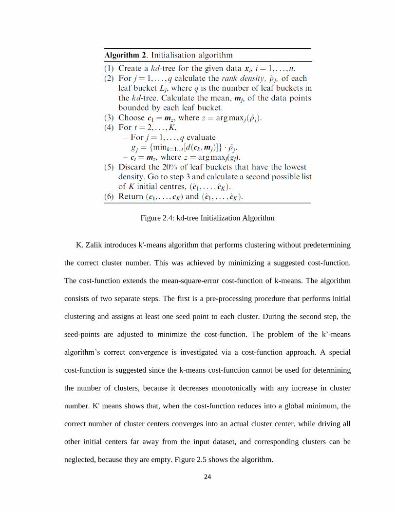
Figure 2.4: kd-tree Initialization Algorithm
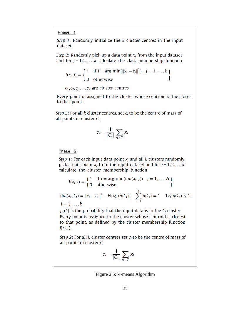
K. Zalik introduces k'-means algorithm that performs clustering without predetermining
the correct cluster number. This was achieved by minimizing a suggested cost-function.
The cost-function extends the mean-square-error cost-function of k-means. The algorithm
consists of two separate steps. The first is a pre-processing procedure that performs initial
clustering and assigns at least one seed point to each cluster. During the second step, the
seed-points are adjusted to minimize the cost-function. The problem of the k’-means
algorithm’s correct convergence is investigated via a cost-function approach. A special
cost-function is suggested since the k-means cost-function cannot be used for determining
the number of clusters, because it decreases monotonically with any increase in cluster
number. K' means shows that, when the cost-function reduces into a global minimum, the
correct number of cluster centers converges into an actual cluster center, while driving all
other initial centers far away from the input dataset, and corresponding clusters can be
neglected, because they are empty. Figure 2.5 shows the algorithm.
25
Figure 2.5: k'-means Algorithm
26
To our best knowledge, the above algorithms are the most recent in the k-means
initialization problem. Although the algorithms show acceptable clustering accuracy, they
suffer from some drawbacks:
1. It takes high execution time to select initial centers, the time complexity for the
IRNN algorithm [17] is exponential since the process of selection and deletion is repeated
many times and in each iteration the RNN degrees, sorting, and deletion are repeated. The
hierarchical initialization approach [14] inherits the same performance disadvantages of
hierarchical clustering [2, 3]. The neighborhood method [20] requires the computation of
cohesion degree for all objects which consumes high execution time.
2. The number of clusters must be previously known and fixed. In some cases the
number of clusters is not known and a method is needed to determine k before clustering.
k'-means algorithm determines k automatically but it suffers from random initialization.
27
Chapter 3: Enhanced k-means
In this chapter, we first introduce some basic definitions used in clustering and then
explain the basic idea of our initialization approach and enhancements of k-means
clustering.
3.1 Some basic definitions
3.1.1 Cohesion degree
Cohesion degree gives critical information about the position of an object in the cluster
[20]; the greater the cohesion degree of an object x the less the boundary region of
neighborhood of object x. Therefore, x is likely taken as an initial cluster center. In order to
compute the cohesion degree for an object x the neighborhood of x and the lower and upper
approximation of a neighborhood set of x should be computed.
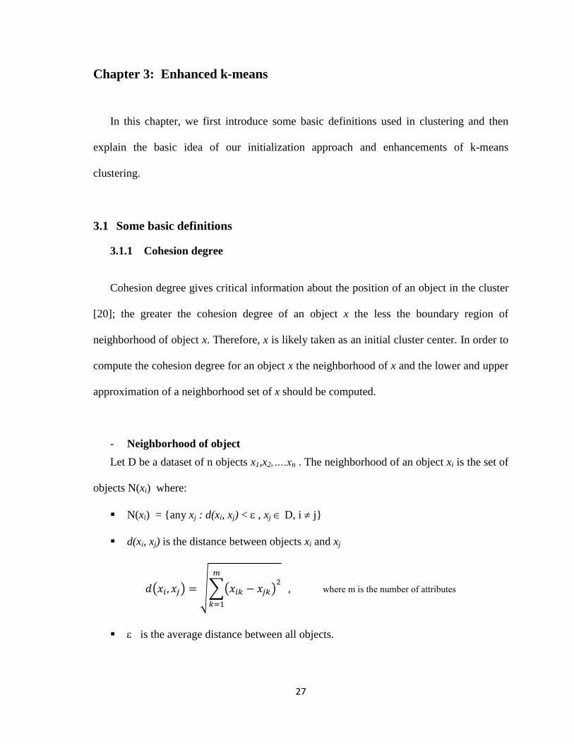
- Neighborhood of object
Let D be a dataset of n objects x1,x2,….xn . The neighborhood of an object xi is the set of
objects N(xi) where:
N(xi) = {any xj : d(xi, xj) < , xj D, i j}
d(xi, xj) is the distance between objects xi and xj
( ) √∑( )
where m is the num er of attri utes
is the average distance between all objects.
28
∑ ∑ ( )
- Lower approximation of a set
Let D be a dataset of n objects x1,x2,….xn and S is a subset of D. The lower
approximation of S (L(S)) is a set of objects whose neighborhood belongs to S with
certainty. In other words, L(S) is the set of objects such that the set of neighbors for each
object belongs to S. Mathematically:
L(S) = { xi : N(xi) S, xi D}
- Upper approximation of a set
Let D be a dataset of n objects x1, x2… xn and S is a subset of D. The upper
approximation of S, (U(S)), is a set of objects whose neighborhood possibly belongs to S.
In other words, U(S) is the set of objects such that the set of neighbors for each object
contains at least one object of S. Mathematically:
U(S) = { xi : N(xi) S , xi D}
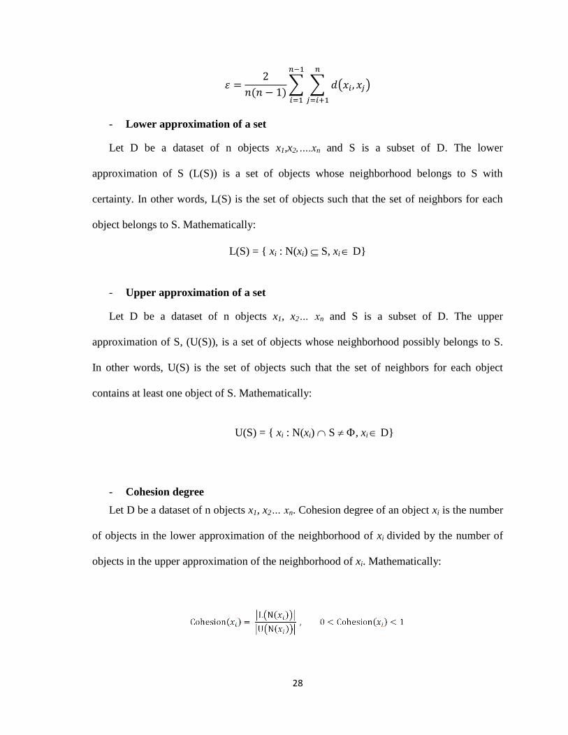
- Cohesion degree
Let D be a dataset of n objects x1, x2… xn. Cohesion degree of an object xi is the number
of objects in the lower approximation of the neighborhood of xi divided by the number of
objects in the upper approximation of the neighborhood of xi. Mathematically:
29
3.1.2 Coupling degree
The coupling degree measures the similarity between two objects. The greater the
coupling degree between two objects the more similar are. So, if two objects are candidate
to be a cluster center, we can reject one of them if the coupling degree between them is high
because they are likely fall in the same cluster. Let D be a dataset of n objects x1, x2… xn.
The coupling degree between neighborhoods of objects xi and xj is the number of objects in
the intersection of the two neighborhoods divided by the number of objects in the union of
the two neighborhoods. Mathematically:
( ( )) | ( )|
| ( )|
( ( ))
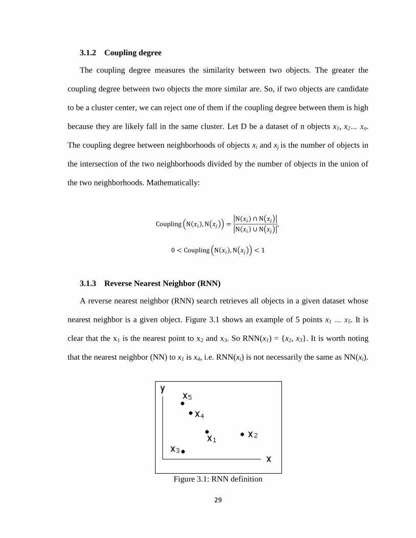
3.1.3 Reverse Nearest Neighbor (RNN)
A reverse nearest neighbor (RNN) search retrieves all objects in a given dataset whose
nearest neighbor is a given object. Figure 3.1 shows an example of 5 points x1 … x5. It is
clear that the x1 is the nearest point to x2 and x3. So RNN(x1) = {x2, x3}. It is worth noting
that the nearest neighbor (NN) to x1 is x4, i.e. RNN(xi) is not necessarily the same as NN(xi).
Figure 3.1: RNN definition
30
The RNN degree of an object is the number of objects retrieved by RNN search. Some
recent studies show that cluster center have high RNN degrees [17]. Let’s clarify this
through figure 3.1. We can easily expect that either x1 or x2 is the cluster center. x1 is the
nearest object to x2, x3, and x4, so RNN degree of x1 is 3. Similarly, the RNN degrees of x2,
x3, x4, and x5 are 0, 0, 2, and 1 respectively. Note that the candidate centers x1 and x4 have
high RNN degrees.
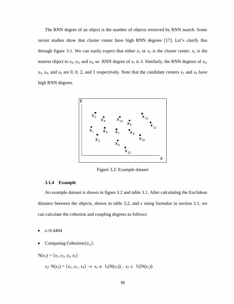
Figure 3.2: Example dataset
3.1.4 Example
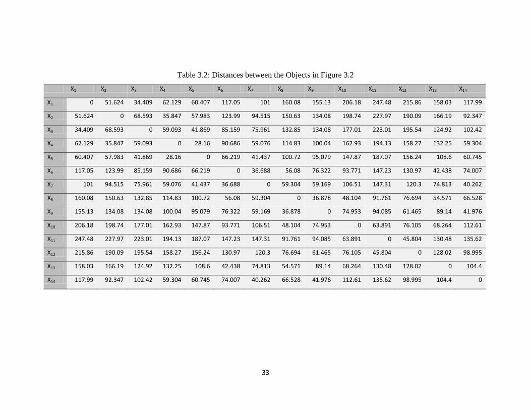
An example dataset is shown in figure 3.2 and table 3.1. After calculating the Euclidean
distance between the objects, shown in table 3.2, and using formulas in section 3.1, we
can calculate the cohesion and coupling degrees as follows:
=0.4404
Computing :
N(x1) = {x1, x2, x3, x5}
x2: N(x2) = {x1, x2 , x4} x2 L(N(x1)) , x2 U(N(x1))
31
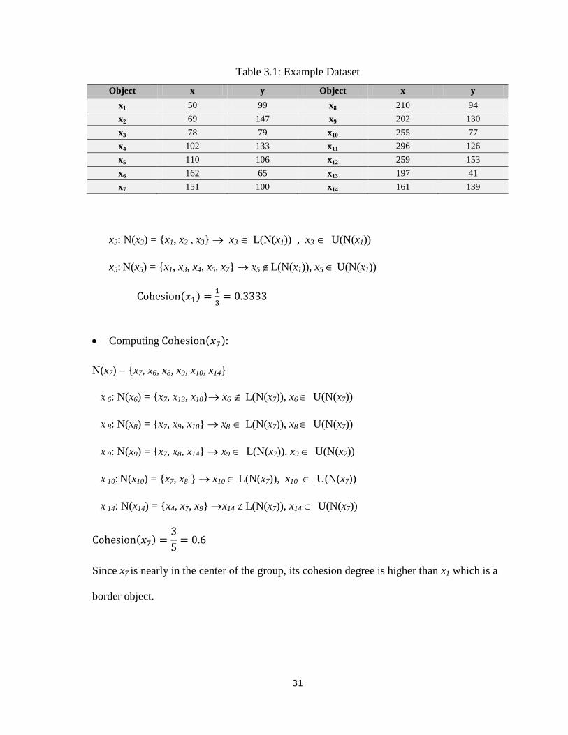
Table 3.1: Example Dataset
Object x y Object x y
x1 50 99 x8 210 94
x2 69 147 x9 202 130
x3 78 79 x10 255 77
x4 102 133 x11 296 126
x5 110 106 x12 259 153
x6 162 65 x13 197 41
x7 151 100 x14 161 139
x3: N(x3) = {x1, x2 , x3} x3 L(N(x1)) , x3 U(N(x1))
x5: N(x5) = {x1, x3, x4, x5, x7} x5 L(N(x1)), x5 U(N(x1))
Computing :
N(x7) = {x7, x6, x8, x9, x10, x14}
x 6: N(x6) = {x7, x13, x10} x6 L(N(x7)), x6 U(N(x7))
x 8: N(x8) = {x7, x9, x10} x8 L(N(x7)), x8 U(N(x7))
x 9: N(x9) = {x7, x8, x14} x9 L(N(x7)), x9 U(N(x7))
x 10: N(x10) = {x7, x8 } x10 L(N(x7)), x10 U(N(x7))
x 14: N(x14) = {x4, x7, x9} x14 L(N(x7)), x14 U(N(x7))
Since x7 is nearly in the center of the group, its cohesion degree is higher than x1 which is a
border object.
32
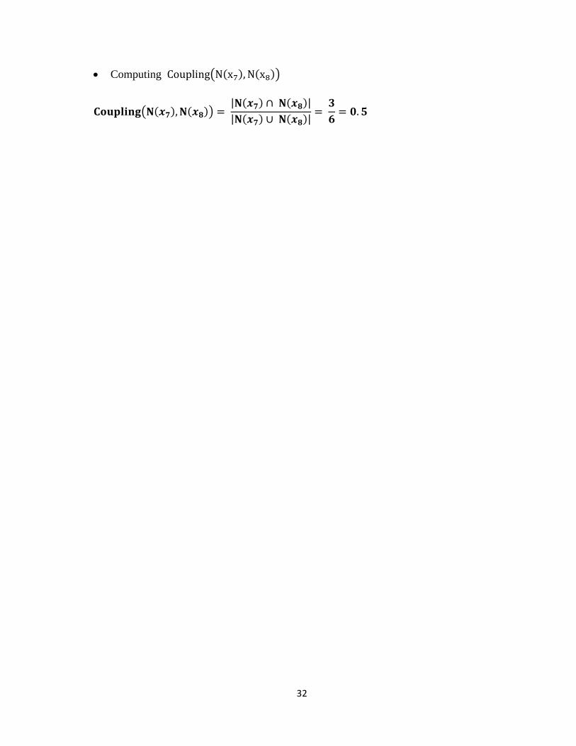
Computing ( )
( )
33
Table 3.2: Distances between the Objects in Figure 3.2
X1 X2 X3 X4 X5 X6 X7 X8 X9 X10 X11 X12 X13 X14
X1 0 51.624 34.409 62.129 60.407 117.05 101 160.08 155.13 206.18 247.48 215.86 158.03 117.99
X2 51.624 0 68.593 35.847 57.983 123.99 94.515 150.63 134.08 198.74 227.97 190.09 166.19 92.347
X3 34.409 68.593 0 59.093 41.869 85.159 75.961 132.85 134.08 177.01 223.01 195.54 124.92 102.42
X4 62.129 35.847 59.093 0 28.16 90.686 59.076 114.83 100.04 162.93 194.13 158.27 132.25 59.304
X5 60.407 57.983 41.869 28.16 0 66.219 41.437 100.72 95.079 147.87 187.07 156.24 108.6 60.745
X6 117.05 123.99 85.159 90.686 66.219 0 36.688 56.08 76.322 93.771 147.23 130.97 42.438 74.007
X7 101 94.515 75.961 59.076 41.437 36.688 0 59.304 59.169 106.51 147.31 120.3 74.813 40.262
X8 160.08 150.63 132.85 114.83 100.72 56.08 59.304 0 36.878 48.104 91.761 76.694 54.571 66.528
X9 155.13 134.08 134.08 100.04 95.079 76.322 59.169 36.878 0 74.953 94.085 61.465 89.14 41.976
X10 206.18 198.74 177.01 162.93 147.87 93.771 106.51 48.104 74.953 0 63.891 76.105 68.264 112.61
X11 247.48 227.97 223.01 194.13 187.07 147.23 147.31 91.761 94.085 63.891 0 45.804 130.48 135.62
X12 215.86 190.09 195.54 158.27 156.24 130.97 120.3 76.694 61.465 76.105 45.804 0 128.02 98.995
X13 158.03 166.19 124.92 132.25 108.6 42.438 74.813 54.571 89.14 68.264 130.48 128.02 0 104.4
X14 117.99 92.347 102.42 59.304 60.745 74.007 40.262 66.528 41.976 112.61 135.62 98.995 104.4 0

34
3.2 An initialization method for the k-Means algorithm using neighborhood
model
In [20], Fuyuan et.al. have presented a method for initializing k-means based on a
neighborhood model. The method defines the cohesion degree of the neighborhood of an
object and the coupling degree between neighborhoods of objects. Then the highest
cohesion degree object is selected as the first center. After that, the coupling degree
between the first center and the next highest degree object is computed and compared; if the
coupling degree is less than some , the next highest degree object is selected as the new
center. Then the steps are repeated till selecting k centers where k is the predefined number
of cluster. The following algorithm finds cluster centers that are passed to k-means
algorithm to group the datasets into a predefined number of clusters, k.
Input: Dataset D, k
Output: k centers
Step1: Compute the distances between objects in D.
Step2: Compute the average distance between all objects .
Step3: Find neighborhood of objects in D.
Step4: Compute Cohesion(xi) for any xi D.
Step5: Find xi: Cohesion(xi) is maximum the first center is found.
Step6: Find the next highest cohesion object xj.
Step7: If Coupling(N(xi),N(xj)):<,next center is found.
Step8: If |centers| < k, go to step 6, otherwise go to step 9.
Step9: End
The time complexity of this algorithm is analyzed as follows. In Step 2, the time
complexity for computing the size of neighborhood is O(n2) where n is the number of
objects in D. Computation of the neighborhood of objects will take O(n2) in Step 3. The
operation on obtaining the most cohering object have a time complexity of O(n) in Step 4.
35
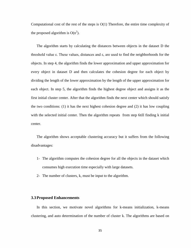
Computational cost of the rest of the steps is O(1) Therefore, the entire time complexity of
the proposed algorithm is O(n2).
The algorithm starts by calculating the distances between objects in the dataset D the
threshold value ε. These values, distances and ε, are used to find the neighborhoods for the
objects. In step 4, the algorithm finds the lower approximation and upper approximation for
every object in dataset D and then calculates the cohesion degree for each object by
dividing the length of the lower approximation by the length of the upper approximation for
each object. In step 5, the algorithm finds the highest degree object and assigns it as the
first initial cluster center. After that the algorithm finds the next center which should satisfy
the two conditions: (1) it has the next highest cohesion degree and (2) it has low coupling
with the selected initial center. Then the algorithm repeats from step 6till finding k initial
center.
The algorithm shows acceptable clustering accuracy but it suffers from the following
disadvantages:
1- The algorithm computes the cohesion degree for all the objects in the dataset which
consumes high execution time especially with large datasets.
2- The number of clusters, k, must be input to the algorithm.
3.3 Proposed Enhancements
In this section, we motivate novel algorithms for k-means initialization, k-means
clustering, and auto determination of the number of cluster k. The algorithms are based on
36
the rough set definitions and the RNN search described above in section 3.1. Section 3.3.1
describes the initialization method. Section 3.3.2 shows how to enhance clustering by
giving high weights to the important attributes. Section 3.3.3 shows the algorithm of
determining k.
3.3.1. Fast k-means Initialization method using Neighborhood and Reverse
Nearest Neighborhood models
In this section a novel initialization algorithm is introduced. The algorithm is built on
the following criteria:
- Clusters centers have high cohesion degrees compared to other objects.
- Clusters centers have low coupling degrees with each other.
- Clusters centers have high RNN degrees.
Based on the above criteria the algorithm below finds appropriate cluster centers that
are passed to k-means algorithm to group the datasets into a predefined number of clusters,
k. The main idea in this algorithm is to combine the criteria of the centers to reduce the
number of objects that the cohesion degree is computed for. We could achieve this by
selecting the m*k objects that have the highest RNN degrees and put them in a set C, where
m is a constant. Then the cohesion degree is computed only for these m*k objects which
reduces the execution time of the algorithm and hence improves performance. This
improvement is noticed clearly when the size of the dataset is large as the results show in
the next chapter. After calculating the cohesion degrees for the objects in C, the highest
cohesion degree object is selected as the first center. After that, the coupling degree
between the first center and the next highest degree object is computed and compared; if the
37
coupling degree is less than some , the next highest degree object is selected as the new
center. Then the steps are repeated till selecting k centers where k is the predefined number
of cluster. We performed experiments to indicate the value of the constant m. We found
that m=3 is a value to give the highest RNN degree objects. However, future work will
concentrate on indicating m through optimizing some function.
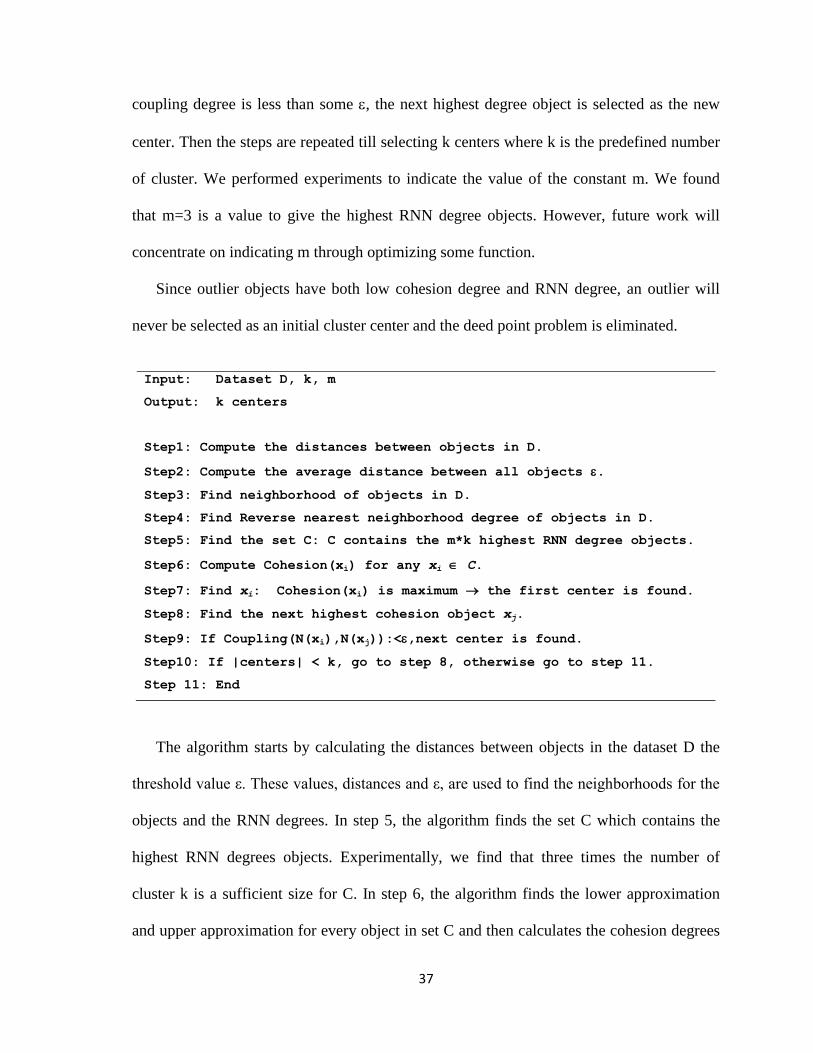
Since outlier objects have both low cohesion degree and RNN degree, an outlier will
never be selected as an initial cluster center and the deed point problem is eliminated.
Input: Dataset D, k, m
Output: k centers
Step1: Compute the distances between objects in D.
Step2: Compute the average distance between all objects .
Step3: Find neighborhood of objects in D.
Step4: Find Reverse nearest neighborhood degree of objects in D.
Step5: Find the set C: C contains the m*k highest RNN degree objects.
Step6: Compute Cohesion(xi) for any xi C.
Step7: Find xi: Cohesion(xi) is maximum the first center is found.
Step8: Find the next highest cohesion object xj.
Step9: If Coupling(N(xi),N(xj)):<,next center is found.
Step10: If |centers| < k, go to step 8, otherwise go to step 11.
Step 11: End
The algorithm starts by calculating the distances between objects in the dataset D the
threshold value ε. These values, distances and ε, are used to find the neigh orhoods for the
objects and the RNN degrees. In step 5, the algorithm finds the set C which contains the
highest RNN degrees objects. Experimentally, we find that three times the number of
cluster k is a sufficient size for C. In step 6, the algorithm finds the lower approximation
and upper approximation for every object in set C and then calculates the cohesion degrees
38
for these objects by dividing the length of the lower approximation by the length of the
upper approximation for each object in C. In step 7, the algorithm finds the highest degree
object and assigns it as the first initial cluster center. After that the algorithm finds the next
center which should satisfy the two conditions: (1) it has the next highest cohesion degree
and (2) it has low coupling with the selected initial center. Then the algorithm repeats from
step 8 till finding k initial center.
The complexity of the algorithm is analyzed as follows. Steps from 1 to 5 have
complexity of O(n2) each, where n is the size of dataset D. The complexity of steps 6 is
O(k2). Steps 7 and 8 have complexity of O(k). Computational cost of the rest of the steps is
O(1). So the overall computational complexity is O(n2).
3.3.2. Auto-determining the number of clusters k using Neighborhood and
Reverse Nearest Neighborhood model
In this section, an algorithm is proposed to determine the number of clusters in a given
dataset based on the following criteria:
- Clusters centers have high cohesion degree compared to other objects.
- Clusters centers have low coupling degree with each other.
- Cluster centers have high RNN degree.
The idea is to find a small subset of objects that fall nearly in the centers of the
supposed clusters. Then this subset is divided into groups based on the coupling degree
between these objects. Objects that have high coupling degree are likely to fall in the same
group while those have low coupling degree fall in different groups. Since objects that fall
39
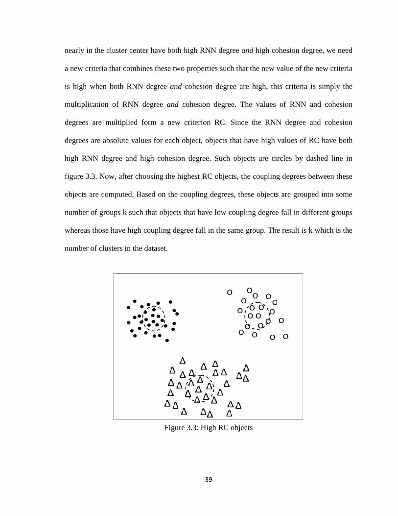
nearly in the cluster center have both high RNN degree and high cohesion degree, we need
a new criteria that combines these two properties such that the new value of the new criteria
is high when both RNN degree and cohesion degree are high, this criteria is simply the
multiplication of RNN degree and cohesion degree. The values of RNN and cohesion
degrees are multiplied form a new criterion RC. Since the RNN degree and cohesion
degrees are absolute values for each object, objects that have high values of RC have both
high RNN degree and high cohesion degree. Such objects are circles by dashed line in
figure 3.3. Now, after choosing the highest RC objects, the coupling degrees between these
objects are computed. Based on the coupling degrees, these objects are grouped into some
number of groups k such that objects that have low coupling degree fall in different groups
whereas those have high coupling degree fall in the same group. The result is k which is the
number of clusters in the dataset.
Figure 3.3: High RC objects
40
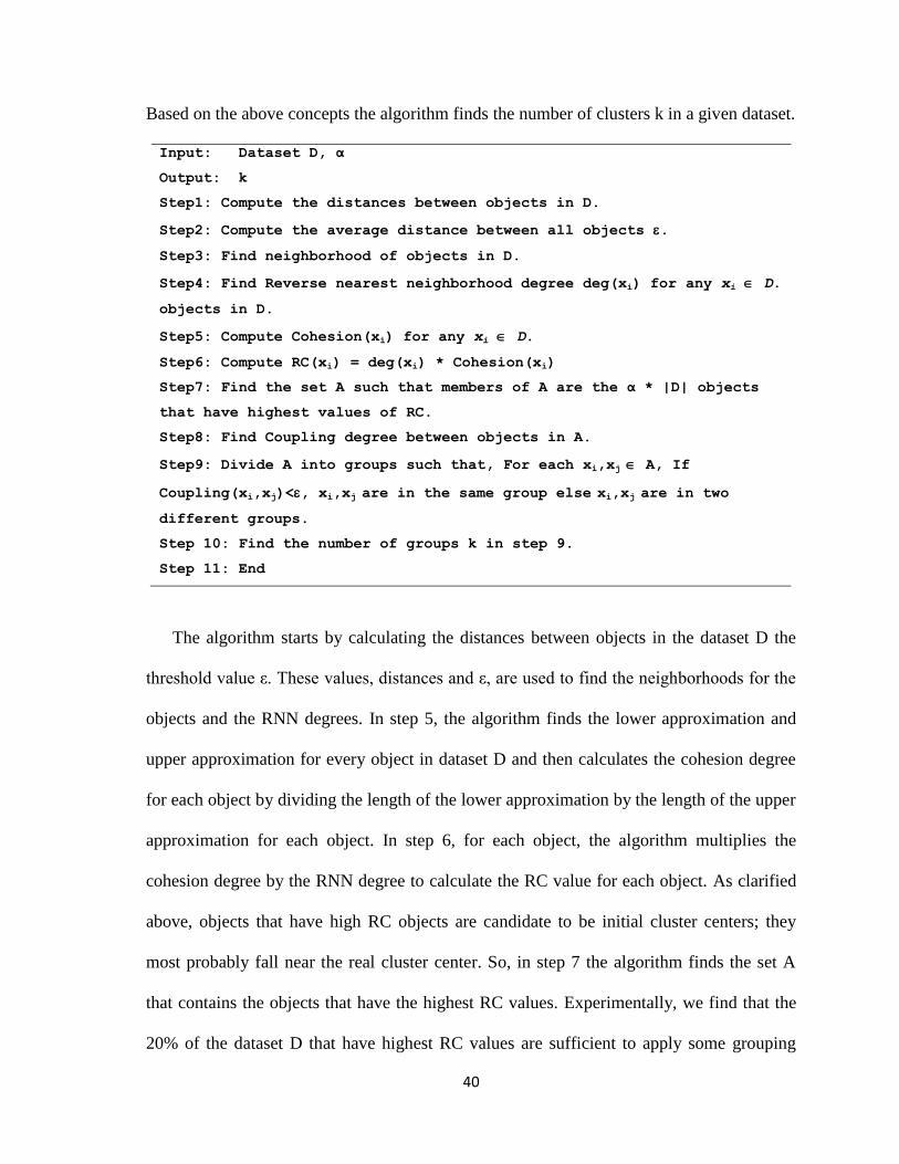
Based on the above concepts the algorithm finds the number of clusters k in a given dataset.
Input: Dataset D, α
Output: k
Step1: Compute the distances between objects in D.
Step2: Compute the average distance between all objects .
Step3: Find neighborhood of objects in D.
Step4: Find Reverse nearest neighborhood degree deg(xi) for any xi D.
objects in D.
Step5: Compute Cohesion(xi) for any xi D.
Step6: Compute RC(xi) = deg(xi) * Cohesion(xi)
Step7: Find the set A such that members of A are the α * |D| objects
that have highest values of RC.
Step8: Find Coupling degree between objects in A.
Step9: Divide A into groups such that, For each xi,xj A, If
Coupling(xi,xj)<, xi,xj are in the same group else xi,xj are in two
different groups.
Step 10: Find the number of groups k in step 9.
Step 11: End
The algorithm starts by calculating the distances between objects in the dataset D the
threshold value ε. These values, distances and ε, are used to find the neigh orhoods for the
objects and the RNN degrees. In step 5, the algorithm finds the lower approximation and
upper approximation for every object in dataset D and then calculates the cohesion degree
for each object by dividing the length of the lower approximation by the length of the upper
approximation for each object. In step 6, for each object, the algorithm multiplies the
cohesion degree by the RNN degree to calculate the RC value for each object. As clarified
above, objects that have high RC objects are candidate to be initial cluster centers; they
most probably fall near the real cluster center. So, in step 7 the algorithm finds the set A
that contains the objects that have the highest RC values. Experimentally, we find that the
20% of the dataset D that have highest RC values are sufficient to apply some grouping
41
method on them to find k. After that, the algorithm finds the coupling degrees between
objects in set A. In step 9, the objects in set A are grouped into groups such that objects
have low coupling degrees fall in different groups while objects have high coupling degrees
fall in the same group while objects. The algorithms outputs the number of groups k which
is the number of clusters in dataset D.
We performed experiments to indicate the value of the constant α. We found that α=0.2
is a sufficient value to give the highest RNN degree objects. However, future work will
concentrate on indicating α through optimizing some function. The complexity of the
algorithm is analyzed as follows. Steps from 1 to 5 have complexity of O(n2) each, where n
is the size of D. The complexity of steps 6 is O(n). Steps 7 has complexity of O(n) [23].
Steps 8 and 9 have complexity of O((α|D|)2). Computational cost of the rest of the steps is
O(1). So the overall computational complexity is O(n2).
42
Chapter 4: Experimental Results
Now, let’s introduce the experiment environments and the results obtained from the
proposed algorithms and the neighborhood model method [20]. The experiments are
performed on a laptop with 1.83 GHz Intel core 2 processor and 1G byte memory running
Windows XP operating systems. MATLAB 7.0 programming language is used to code the
algorithms.
4.1 Results of Initialization algorithms
To compare the two initialization methods four datasets are used; three standard
datasets and one test dataset. The three standard datasets are Iris, Wine, and Glass [22]. We
performed experiments to indicate the value of the constant m. We found that m=3 is a
sufficient value to give the highest RNN degree objects.
To evaluate the performance of the two initialization methods three evaluation criteria
are employed, accuracy (AC), execution time (exeTime), and the number of iterations that
k-means needs to converge. AC is the ratio between the number of objects that are assigned
correctly to their clusters and the size of the dataset. Execution time measures the
performance of the algorithms. Low execution time means that the algorithm performs
faster. The convergence iterations indicate the accuracy of the initialization method. Low
number of convergence iterations indicates that the initial centers are selected accurately
i.e. near the real centers.
Iris dataset: Iris dataset is a standard dataset. It contains three classes that represent three
types of Iris flowers namely, Iris setosa, Iris versicolor and Iris virginica. Iris dataset
contains 150 objects divided equally between the three classes. Each object is represented
43
by four attributes namely, viz sepal length, sepal width, petal length and petal width.
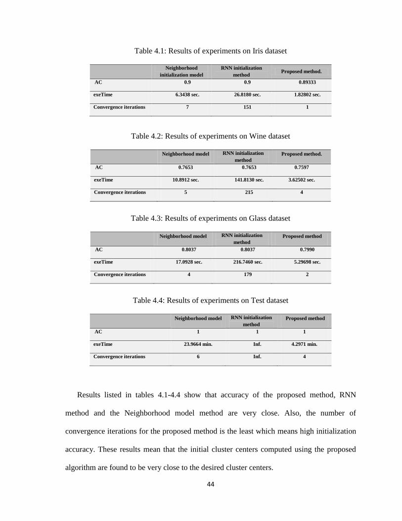
Table 4.1 shows the experimental results on the Iris dataset.
Wine dataset: Wine dataset is a standard dataset. It contains three classes that represent
chemical results on wines derived from three different cultivars. Wine dataset contains
178 objects. There are 59, 71, 48 objects in class 1, class 2 and class 3 respectively. Each
object is represented by 13 attributes. Table 4.2 shows the experimental results on the
Wine dataset.
Glass dataset: Glass dataset is a standard dataset that contains seven classes namely,
building windows, vehicle windows, building windows, vehicle windows, containers,
tableware and headlamps. Glass dataset contains 214 objects. There are 70, 17, 76, 0, 13,
9, 29 objects in classes 1 to 7 respectively. Each object is represented by 10 attributes.
Table 4.3 shows the experimental results on the Glass dataset.
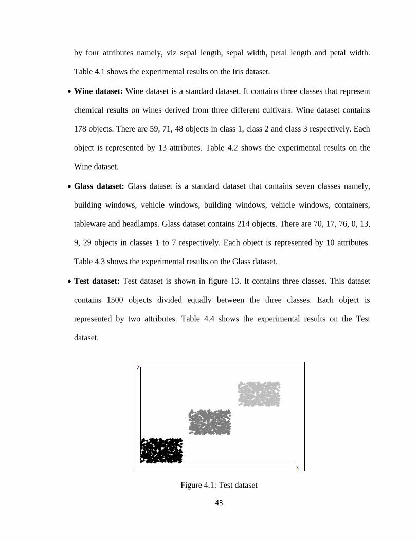
Test dataset: Test dataset is shown in figure 13. It contains three classes. This dataset
contains 1500 objects divided equally between the three classes. Each object is
represented by two attributes. Table 4.4 shows the experimental results on the Test
dataset.
Figure 4.1: Test dataset
44
Table 4.1: Results of experiments on Iris dataset
Neighborhood
initialization model
RNN initialization
method Proposed method.
AC 0.9 0.9 0.89333
exeTime 6.3438 sec. 26.8180 sec. 1.82802 sec.
Convergence iterations 7 151 1
Table 4.2: Results of experiments on Wine dataset
Neighborhood model RNN initialization
method
Proposed method.
AC 0.7653 0.7653 0.7597
exeTime 10.8912 sec. 141.8130 sec. 3.62502 sec.
Convergence iterations 5 215 4
Table 4.3: Results of experiments on Glass dataset
Neighborhood model RNN initialization
method
Proposed method
AC 0.8037 0.8037 0.7990
exeTime 17.0928 sec. 216.7460 sec. 5.29698 sec.
Convergence iterations 4 179 2
Table 4.4: Results of experiments on Test dataset
Neighborhood model RNN initialization
method
Proposed method
AC 1 1 1
exeTime 23.9664 min. Inf. 4.2971 min.
Convergence iterations 6 Inf. 4
Results listed in tables 4.1-4.4 show that accuracy of the proposed method, RNN
method and the Neighborhood model method are very close. Also, the number of
convergence iterations for the proposed method is the least which means high initialization
accuracy. These results mean that the initial cluster centers computed using the proposed
algorithm are found to be very close to the desired cluster centers.
45
The proposed method outperforms the Neighborhood model method and RNN. The
reason behind this improvement is that the proposed algorithm employs both the cohesion
degree and RNN degree to compute the initial center. The computation of the cohesion
degree is time consuming since it requires computing many values such as neighborhood,
lower approximation and upper approximation for each object. The RNN degree limits the
number of objects that we need to compute the cohesion degree for.
4.2 Results of Auto-determining k
In this section we introduce the results of applying the algorithm of auto-determination
of k. The constant α in the algorithm was indicated experimentally α=0.2. The algorithm is
applied on the following datasets:
Iris dataset: Iris dataset is a standard dataset. It contains three classes that represent three
types of Iris flowers namely, Iris setosa, Iris versicolor and Iris virginica. Iris dataset
contains 150 objects divided equally between the three classes. Each object is represented
by four attributes namely, viz sepal length, sepal width, petal length and petal width [20].
s2: Synthetic 2-d data with 5000 vectors and 15 Gaussian clusters [24]
Teaching Assistant Evaluation dataset: The data consist of evaluations of teaching
performance over three regular semesters and two summer semesters of 151 teaching
assistant (TA) assignments at the Statistics Department of the University of Wisconsin-
Madison. The scores were divided into 3 roughly equal-sized categories. [22]
46
Blood Transfusion Service Center dataset: Data taken from the Blood Transfusion
Service Center in Hsin-Chu City in Taiwan. It contains two clusters, 748 objects, and 4
attributes [22].
Haberman's Survival dataset: The dataset contains cases from a study that was
conducted between 1958 and 1970 at the University of Chicago's Billings Hospital on
the survival of patients who had undergone surgery for breast cancer. It contains three
clusters, 30 objects, and 4 attributes [22].
Wine dataset: Wine dataset is a standard dataset. It contains three classes that represent
chemical results on wines derived from three different cultivars. Wine dataset contains
178 objects. There are 59, 71, 48 objects in class 1, class 2 and class 3 respectively. Each
object is represented by 13 attributes [20].
Glass dataset: Glass dataset is a standard dataset that contains seven classes namely,
building windows, vehicle windows, building windows, vehicle windows, containers,
tableware and headlamps. Glass dataset contains 214 objects. There are 70, 17, 76, 0, 13,
9, 29 objects in classes 1 to 7 respectively. Each object is represented by 10 attributes
[20].
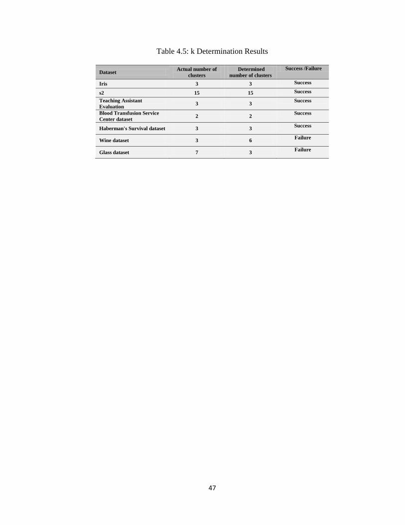
Table 4.5 lists the results of executing the k determination algorithm on the above
datasets. The results show that the algorithm fails in case of high dimension datasets such
as wine and glass datasets. Since k-means algorithm works well with low dimension
datasets and not high dimension ones, the k determination algorithm can be helpful to be
used with k- means.
47
Table 4.5: k Determination Results
Dataset Actual number of
clusters
Determined
number of clusters
Success /Failure
Iris 3 3 Success
s2 15 15 Success
Teaching Assistant
Evaluation 3 3
Success
Blood Transfusion Service
Center dataset 2 2
Success
Haberman's Survival dataset 3 3 Success
Wine dataset 3 6 Failure
Glass dataset 7 3 Failure
48
Chapter 5: Conclusion and Future work
The simplicity of k-means algorithm makes it the choice for many clustering tasks.
However k-means suffers from the problems of random initialization, dead point problem,
and the predetermined of number of clusters k. Based on some basic concepts of the rough
set theory and the reverse nearest neighbor search method we introduced a novel
initialization algorithm that performs well to find appropriate initial centers for the k-means
clustering. The experimental results illustrate the advantages of the proposed initialization
method which are (1) high clustering accuracy, (2) fast convergence and (3) fast execution.
The proposed algorithm also eliminates dead point problem. Results show also that rough
set theory concepts can be employed to determine the number of clusters k.
Currently, two constants were indicated experimentally, m in the initialization
enhancement and α in the k auto-determination algorithm. An extension of the work would
be to come up with a formula for choosing the appropriate threshold values, a formula that
would work for all dimensions, number of points and centers. Here we have only been able
to experimentally see that an optimum threshold value exists, but not been able to come to
the exact value. It is also likely that the thresholds depend on the type of data. More
research is needed for deriving the formula.

49
References
[1] S. Theodoridis and k. Koutroumbaspattern, Pattern Recognition, 2nd
edition, Elsevier,
2003.
[2] G. Gan et. al, Data Clustering Theory, Algorithms, and Applications, Siam, 2007.
[3] J. Han and M. Kamber, Data Mining: Concepts and Techniques, 2nd
edition, Elsevier,
2006.
[4] J. MacQueen, "Some methods for classification and analysis of multivariate
observation". In: Berkeley Symposium on Mathematical Statistics and Probability.
University of California Press, pp. 281–297, 1967.
[5] L. Kaufman and P. Rousseeuw. Finding Groups in Data: An Introduction to Cluster
Analysis. Wiley, New York, 1990.
[6] T. Zhang et. al. "BIRCH: An efficient data clustering method for very large databases".
In Proceedings of the 1996 ACM SIGMOD international conference on management of
data, pp. 103–114. New York: ACM Press, 1996.
[7] M. Ester et. al., "A density-based algorithm for discovering clusters in large spatial
databases with noise," In Second international conference on knowledge discovery and data
mining", pp. 226–231. Portland, OR: AAAI Press, 1996.
[8] M. Ankerst et. al, "OPTICS: Ordering points to identify the clustering structure," In
Proc. 1999 ACM-SIGMOD Int. Conf.Management of Data(SIGMOD’99), pp. 49–60,
Philadelphia, 1999.
[9] W. Wang et. al, "STING: A statistical information grid approach to spatial data
mining," In Twenty-third international conference on very large data bases, pp. 186–195,
1997.
50
[10] R. Agrawal et. al, "Automatic subspace clustering of high dimensional data for data
mining applications," In SIGMOD Record ACM Special Interest Group on Management of
Data, pp. 94–105. New York: ACM Press. 1998.
[11] D. Fisher. "Improving inference through conceptual clustering," In Proc. 1987 Nat.
Conf. Artificial Intelligence (AAAI’87), pp. 461–465, Seattle,WA, 1987.
[12] T. Kohonen, "The self-organizing map," Proceedings of the IEEE, 78(9):1464–1480,
1990.
[13] S. Redmond and C. Heneghan, "A method for initializing the k-means clustering
algorithm using kd-trees," Pattern Recognition Letters, vol. 28, issue 8, pp. 965–973, 2007.
[14] J. Lu. et. al, "Hierarchical initialization approach for k-Means clustering," Pattern
Recognition Letters, vol. 29, pp. 787–795, 2008.
[15] S. Khan and A. Ahmad, "Cluster center initialization algorithm for k-means
clustering," Pattern Recognition Letters, vol. 25, pp. 1293–1302, 2004.
[16] A. Likas et. al, "The global k-means clustering algorithm," Pattern Recognition, vol.
36, pp. 451 – 461, 2003.
[17] X. Junling et. al, "Stable Initialization Scheme for k-Means Clustering," Wuhan
University Journal Of Natural Sciences, vol.14, no.1, 2009.
[18] T. Su and J. Dy, "A Deterministic Method for Initializing k-means Clustering",
Proceedings of the 16th IEEE International Conference on Tools with Artificial Intelligence
(ICTAI 2004), 15-17 Nov, pp. 784 – 786, 2004.
[19] J. Pena et. al, "An empirical comparison of four initialization methods for the k-Means
algorithm," Pattern Recognition Letters, vol. 20, pp. 1027-1040, 1999.
51
[20] F. Caoa et. al., "An initialization method for the k-Means algorithm using
neighborhood model", Computers and Mathematics with Applications, vol. 58, pp. 474 –
483, 2009.
[21] Z. Pawlak, "Rough Sets-Theoretical Aspects of Reasoning about Data", Kluwer
Academic Publishers, Dordrecht, Boston, London, 1991.
[22] A. Asuncion and D.J. Newman, University of Califirnia, Dept. of Informayion and
Computer Science. The UCI Machine Learning Repository
http://mlearn.ics.uci.edu/MLRepository.html. Last visit Oct. 11, 2010.
[23] Mathwoorks, Min/Max selection,
http://www.mathworks.com/matlabcentral/fileexchange/23576-minmax-selection. Last visit
Oct. 11, 2010.
[24] Clustering datasets, University of Eastern Finland, http://cs.joensuu.fi/sipu/datasets/.
Last Visit Oct. 11, 2010
[25] H.Wang et. al., “Clustering y pattern similarity in large data sets,” Proc. ACM
SIGMOD Int. Conf. Management of Data, pp. 394–405, 2002.
[26] P. Tan, M. Steinbach and V. Kumar, Introduction to Data Mining, 1st edition, Addison-
Wesley, 2006.
[27] S. J. Redmond and C. Heneghan, “A method for initialising the K-means clustering
algorithm using kd-trees ", Pattern Recognition Letters, no. 28, pp. 965–973, 2007.
[28] P.S. Bradley and U. M. Fayyad, "Refining initial points for k-means clustering." In
Proceedings Fifteenth International Conference on Machine Learning, pp. 91-99, San
Francisco, CA, 1998, Morgan Kaufmann.
52
[29] A. W. Moore, "An introductory tutorial on kd-trees", PhD Thesis: Efficient Memory-
based learning for Robot Control, PhD Thesis; Technical Report No. 209, Computer
Laboratory, University of Cambridge, 1991.
[30] D. Pelleg and A. Moore, "X-means: Extending k-means with efficient estimation of the
number of clusters". In Proceedings of the Seventeenth International Conference on
Machine Learning, Palo Alto, CA, July 2000.