Prepared for submission to JHEP MIT-CTP-4645

Enhanced gauge symmetry in 6D F-theory modelsand tuned elliptic Calabi-Yau threefolds

Samuel B. Johnson and Washington TaylorCenter for Theoretical PhysicsDepartment of PhysicsMassachusetts Institute of Technology77 Massachusetts AvenueCambridge, MA 02139, USA

samj at mit.edu ; wati at mit.edu

Abstract: We systematically analyze the local combinations of gauge groups and matterthat can arise in 6D F-theory models over a fixed base. We compare the low-energy con-straints of anomaly cancellation to explicit F-theory constructions using Weierstrass and Tateforms, and identify some new local structures in the “swampland” of 6D supergravity andSCFT models that appear consistent from low-energy considerations but do not have knownF-theory realizations. In particular, we classify and carry out a local analysis of all enhance-ments of the irreducible gauge and matter contributions from “non-Higgsable clusters,” andon isolated curves and pairs of intersecting rational curves of arbitrary self-intersection. Suchenhancements correspond physically to unHiggsings, and mathematically to tunings of theWeierstrass model of an elliptic CY threefold. We determine the shift in Hodge numbers ofthe elliptic threefold associated with each enhancement. We also consider local tunings oncurves that have higher genus or intersect multiple other curves, codimension two tunings thatgive transitions in the F-theory matter content, tunings of abelian factors in the gauge group,and generalizations of the “E8” rule to include tunings and curves of self-intersection zero.These tools can be combined into an algorithm that in principle enables a finite and system-atic classification of all elliptic CY threefolds and corresponding 6D F-theory SUGRA modelsover a given compact base (modulo some technical caveats in various special circumstances),and are also relevant to the classification of 6D SCFT’s. To illustrate the utility of theseresults, we identify some large example classes of known CY threefolds in the Kreuzer-Skarkedatabase as Weierstrass models over complex surface bases with specific simple tunings, andwe survey the range of tunings possible over one specific base.

arX

iv:1

605.

0805

2v2

[he

p-th

] 1

6 Ju

n 20

16

Contents

1 Introduction 1

2 Physical and geometric background 42.1 F-theory preliminaries 42.2 Algebraic geometry preliminaries 72.3 6D supergravity 112.4 6D SCFTs 132.5 Calabi-Yau threefolds 15

3 Outline of results 17

4 Classification I: isolated curves 194.1 Extended example: tunings on a −3 curve 21

4.1.1 Spectrum and Hodge shifts from anomaly cancellation 214.1.2 Spectrum and Hodge shifts from local geometry 24

4.2 Special case: tuning so(N > 8) 274.2.1 Spectrum and Hodge shifts from anomaly cancellation 294.2.2 Spectrum and Hodge shifts from local geometry 30

4.3 Tuning on rational curves of self-intersection n ≥ −2 334.3.1 Tuning exceptional algebras on n ≥ −2 curves 334.3.2 Tuning su(N) and sp(N) on n ≥ −2 curves 344.3.3 Tuning so(N) on n ≥ −2 curves 36

4.4 Higher genus curves 37

5 Classification II: multiple-curve clusters 385.1 The clusters (−3,−2,−2), (−2,−3,−2), and (−3,−2) 385.2 −2 clusters 39

5.2.1 Linear −2 chains 405.2.2 Nonlinear −2 clusters 425.2.3 Tuning other groups on −2 curve clusters: special cases 44

6 Classification III: connecting curves and clusters 486.1 Types of groups on intersecting divisors 496.2 Constraining groups on intersecting divisors 516.3 Multiple curves intersecting Σ 566.4 No gauge group on Σ (generalizing the “E8 rule”) 586.5 More general intersection structures 61

7 Tuning exotic matter 61

– i –

8 Tuning abelian gauge factors 638.1 Single abelian factors 648.2 Multiple U(1)’s 668.3 Discrete abelian gauge factors 67

9 A tuning algorithm 689.1 The algorithm 689.2 Open questions related to the classification algorithm 70

10 Examples 7210.1 Example: two classes of tuned elliptic fibrations in Kreuzer-Skarke 7310.2 Example: tunings on F12 74

11 Conclusions and Outlook 7911.1 Summary of results 7911.2 The 6D N = 1 “tuning” swampland 8111.3 Tate vs. Weierstrass 8311.4 4D F-theory models 8311.5 Outstanding questions 84

A Tabulated results 86

B Tabulations of group theory coefficients 90

C Complete HC Calculations 91C.1 The Cluster (-3,-2) 91C.2 The Cluster (−3,−2,−2) 93C.3 The Cluster (-2,-3,-2) 94C.4 The Cluster (-4) 95C.5 The Cluster (-5) 96C.6 The Cluster (-6) 96C.7 The Clusters (-7), (-8), and (-12) 96

1 Introduction

Compactifications have long played a fundamental role within string theory, beginning asa necessary ingredient for approaching 4D phenomenology. Evolving perspectives on stringtheory have yielded increasingly rich classes of compactifications. With the advent of F-theory [1, 2], a spatially varying axio-dilaton profile in type IIB string theory has enabledthe construction of lower-dimensional theories with a wide range of gauge symmetries and

– 1 –

matter content in a non-perturbative and unifying framework. In recent years, followingextensive work on increasingly phenomenologically coherent F-theory GUT models [3, 4], therehas been a renaissance of work on both phenomenological and more foundational aspectsof F-theory. For 4D N = 1 F-theory constructions, fluxes produce a superpotential thatlifts many moduli; non-perturbative 7-brane world-volume dynamics are difficult to control;and other constructions appear to give large classes of vacua with no F-theory dual. Thesedifficulties render the exploration and global understanding of the full set of 4D N = 1

compactifications quite subtle. In 6D, on the other hand, the class of models resulting fromF-theory compactifications is tightly controlled. In particular, there is a very close connectionbetween the geometry of complex surfaces and the physics of 6D supergravity theories; forexample, low-energy consistency conditions such as the Green-Schwarz mechanism of anomalycancellation [5, 6], which are quite stringent, can be mapped directly to geometric constraints[7–11].

The moduli space of 6D supergravities arising from F-theory compactifications is a con-nected space, with different branches connected through superconformal fixed points by ten-sionless string transitions [12, 2, 9]. The possibility of a complete and explicit descriptionof this space seems in principle feasible. F-theory compactifications to 6D are realized bycompactifying type IIB string theory on a complex surface base B that supports an ellipticCalabi-Yau threefold. In recent work, significant progress has been made on a systematicclassification of all possible such compact smooth base surfaces B [13–16]. If one can in ad-dition understand the allowed tunings of different elliptic fibrations over each of these bases,corresponding to F-theory models with distinct spectra, one would have a very clear handle onthis moduli space. Some progress in this direction was made in [17]. One of the primary goalsof this paper is to expand the set of tools for the systematic understanding of such tunings,which correspond physically to enhancing the gauge and matter content of the supergravitymodel. Recently, similar methods have been used to explore six-dimensional superconfor-mal field theories (SCFT’s) [18, 19]. These non-compact F-theory models are in some wayssimpler, yet in other ways less constrained, than their supergravity counterparts; for thesetheories as well, the classification problem can be divided into two independent sub-problems:the classification of the base geometry, and the classification of tuned enhancements of gaugesymmetry and matter content, given a base geometry. Parts of this paper that are relevantto SCFT’s have significant overlap with [19], which appeared while this work was in progress.

Mathematically, the classification of 6D F-theory models corresponds to the classificationof Weierstrass models for elliptic Calabi-Yau threefolds. Every elliptic Calabi-Yau threefoldhas a Weierstrass model realization [20], so this problem is tantamount to (though slightlydistinct from) the problem of classifying elliptic Calabi-Yau threefolds. The minimal modelprogram for surfaces and the work of Grassi [21] show that all base surfaces that supportelliptic CY threefolds can be constructed as blow-ups of a small finite set of minimal surfaces.It was proven by Gross [22] that the number of birational equivalence classes of ellipticallyfibered Calabi-Yau threefolds is finite. A more constructive argument was given in [9], whichshows that there are a finite number of distinct families of Weierstrass models corresponding

– 2 –

to distinct 6D F-theory spectra; these Weierstrass models can be in principle classified by firstconstructing all bases B and then finding all allowed tunings over each B. It is the latterproblem, of tuning Weierstrass models over a given base B, that we address in the presentwork.

There are thus three distinct classification problems that we wish to make progress towardsby the systematic study of allowed tunings in 6D F-theory models: First, the classification ofelliptic Calabi-Yau threefolds; second, the related classification of 6D supergravity models; andthird, the classification of 6D SCFT’s. It has been conjectured that all quantum consistent 6Dsupergravity theories and all 6D superconformal field theories have realizations in F-theory[23, 8, 18]. Thus, a complete classification of allowed tunings may help to solve all three of theseclassification problems. While we do not completely solve these classification problems here,we develop a systematic description of possible local tunings, which we incorporate into analgorithmic framework for approaching these problems, with unresolved issues isolated intospecific technical questions that can be addressed in further work. Throughout the paper,we also identify and focus particular attention on theories in the “swampland” [24], which areapparently consistent from low-energy considerations, yet do not have an F-theory description.

The outline of this paper is the following. We first review the basics of F-theory construc-tions in §2, including the traditional interpretation in terms of a IIB theory with a varyingaxio-dilaton profile. We review the structure of non-Higgsable clusters, 6D supergravity, and6D SCFTs. We also include a brief review of some aspects of algebraic geometry and toricgeometry, setting notation for the following calculations. In §3, we present a more in-depthsummary of our classification strategy, the components of which are developed in the followingsections. Sections §4 through §6 contain the core results of the paper: they consist respectivelyof constraints for tunings of enhanced gauge groups on isolated divisors (curves), constraintsfor tunings on multiple-divisor clusters, and constraints determining when two or more of thepreviously discussed tunings may be achieved simultaneously. These constraints are all localin that they require the simultaneous consideration of local configurations of intersecting di-visors in the base. For many of these cases, particularly those where the curves involved forma non-Higgsable cluster, we explicitly check that local models for all of the possible gaugegroups allowed by the constraints can be realized explicitly by tuning monomials in a Weier-strass model. In §7 and §8 we describe the tunings of exotic matter and abelian gauge factors,which go beyond the simple Kodaira classification of gauge groups and generic matter. In §9,we assemble all these pieces into a systematic algorithm for determining a finite set of possibleWeierstrass models over a given base. In some cases, this list may represent a superset of thetrue set of allowed F-theory models; certain combinations of local structures must be checkedexplicitly to verify the existence of a global Weierstrass model. In §10, we illustrate the utilityof these rules by investigating two classes of tuned models in the Kreuzer-Skarke database,and exploring the range of tunings possible over the Hirzebruch surface base B = F12. Lastly,§11 reviews our results and their limitations, and explores some potentially interesting futuredirections.

As this paper was in the final stages of completion, we learned of independent concurrent

– 3 –

work by Morrison and Rudelius [25] that also considers the generalization of the E8 rule totuned gauge groups.

2 Physical and geometric background

2.1 F-theory preliminaries

We begin with a brief review of some basic aspects of F-theory; more extensive pedagogicalintroductions can be found in [26–28]. In its original form, F-theory [1, 2] is an attempt tocapture and codify geometrically the SL(2,Z) S-symmetry of type IIB string theory in a waythat greatly broadens the class of manifolds on which the IIB theory can be compactifiedwhile preserving symmetry, by allowing variation of the axiodilaton field τ := C0 + ie−φ tocompensate for curvature in the compactification space. Under the IIB SL(2,Z) symmetry,the axiodilaton transforms as

τ → τ ′ =aτ + b

cτ + d(2.1)

for ab− cd = ±1 (all four constants in Z). Because the true moduli space of IIB is a quotientof the τ plane by this symmetry, and this is nothing but the (complex) moduli space of thetorus, the axiodilaton at each point in space-time can be identified with an elliptic curve E.Allowing this coupling to depend on position yields an elliptic fibration (with a well definedglobal zero-section) over the compact space B of the IIB compactification. In practice, whenwe form an F-theory model by starting with the IIB theory compactified on a “base” B, withvarying axio-dilaton profile as above, as a shorthand we say “F-theory compactified on X”where X is the total space of the elliptic fibration E ↪→ X

π→ B.The study of F-theory is morally the study of elliptically fibered (with section) Calabi-Yau

manifolds. (Throughout this paper, we focus on (complex) threefolds.) Essential physical dataof the resulting low-energy theory on R1,5 are encoded in the singularities of the elliptic fibra-tion, namely the loci where one or both cycles of the torus degenerate. Because singularitiesin the elliptic fibration are accompanied by monodromies of τ , it is natural to interpret thesesingularity loci as the support of 7-branes within the theory. In terms of the two generators

T1 =

(1 1

0 1

)and T2 =

(0 1

−1 0

)of SL(2,Z), a monodromy of pT1 + qT2 corresponds to a

so-called (p, q) 7-brane. (Only the familiar (1, 0) D7 brane is visible in perturbative IIB stringtheory.) Just as it was discovered early on that when a stack of parallel D-branes coincide,the open strings stretched between them have endpoint degrees of freedom that fill out thegauge sector of an SU(N) gauge theory; so too was it realized that these generalized branescould encode more general gauge symmetries. Although many perspectives exist on this result([2, 27]), the most useful is a long-known mathematical result that completely characterizescodimension one singularities of elliptic fibrations: the Kodaira classification (see e.g. [29]).

To discuss the Kodaira classification, it is necessary to recall a convenient description ofan elliptic curve. In the weighted projective space P[2,3,1], an elliptic curve can be written in

– 4 –

Type ord (f) ord (g) ord (∆) singularity nonabelian symmetry algebra

I0 ≥ 0 ≥ 0 0 none noneIn 0 0 n ≥ 2 An−1 su(n) or sp(bn/2c)II ≥ 1 1 2 none noneIII 1 ≥ 2 3 A1 su(2)

IV ≥ 2 2 4 A2 su(3) or su(2)

I∗0 ≥ 2 ≥ 3 6 D4 so(8) or so(7) or g2

I∗n 2 3 n ≥ 7 Dn−2 so(2n− 4) or so(2n− 5)

IV ∗ ≥ 3 4 8 e6 e6 or f4III∗ 3 ≥ 5 9 e7 e7

II∗ ≥ 4 5 10 e8 e8

non-min ≥ 4 ≥ 6 ≥ 12 does not occur in F-theory

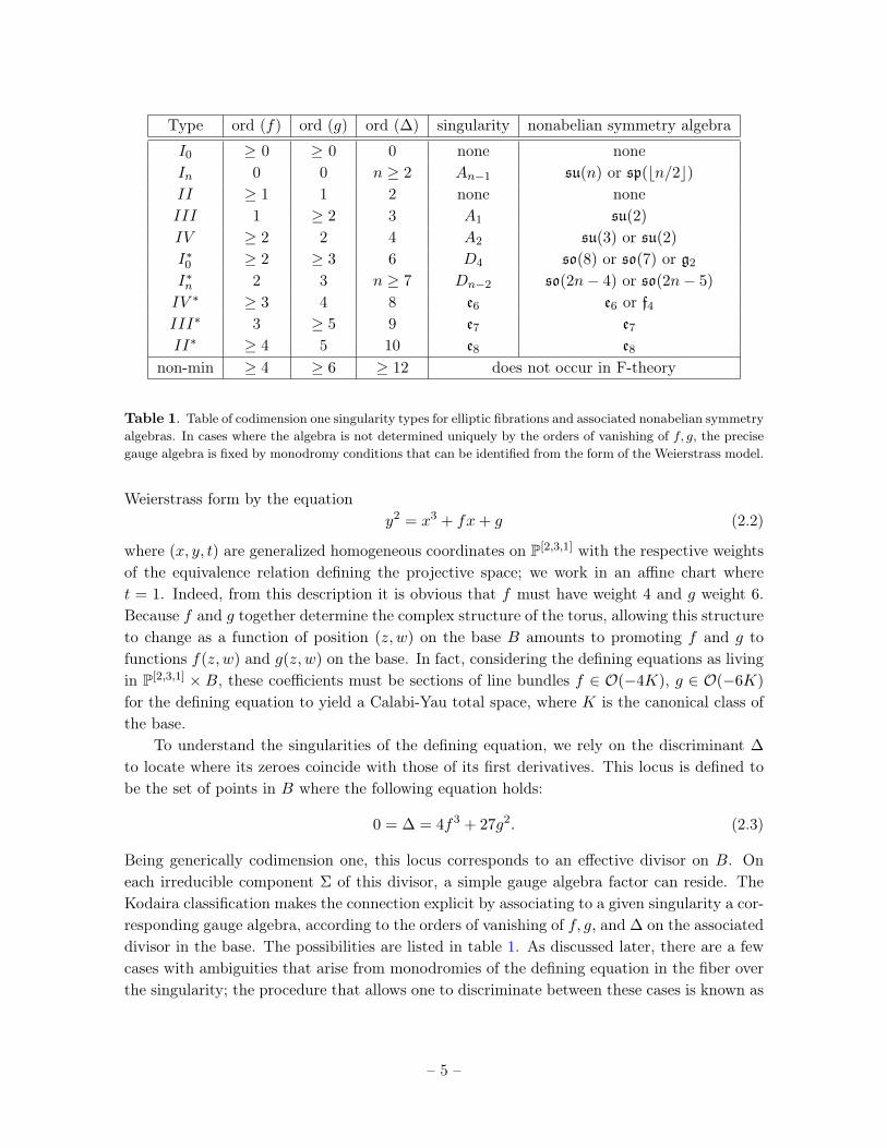
Table 1. Table of codimension one singularity types for elliptic fibrations and associated nonabelian symmetryalgebras. In cases where the algebra is not determined uniquely by the orders of vanishing of f, g, the precisegauge algebra is fixed by monodromy conditions that can be identified from the form of the Weierstrass model.

Weierstrass form by the equationy2 = x3 + fx+ g (2.2)

where (x, y, t) are generalized homogeneous coordinates on P[2,3,1] with the respective weightsof the equivalence relation defining the projective space; we work in an affine chart wheret = 1. Indeed, from this description it is obvious that f must have weight 4 and g weight 6.Because f and g together determine the complex structure of the torus, allowing this structureto change as a function of position (z, w) on the base B amounts to promoting f and g tofunctions f(z, w) and g(z, w) on the base. In fact, considering the defining equations as livingin P[2,3,1] × B, these coefficients must be sections of line bundles f ∈ O(−4K), g ∈ O(−6K)

for the defining equation to yield a Calabi-Yau total space, where K is the canonical class ofthe base.

To understand the singularities of the defining equation, we rely on the discriminant ∆

to locate where its zeroes coincide with those of its first derivatives. This locus is defined tobe the set of points in B where the following equation holds:

0 = ∆ = 4f3 + 27g2. (2.3)

Being generically codimension one, this locus corresponds to an effective divisor on B. Oneach irreducible component Σ of this divisor, a simple gauge algebra factor can reside. TheKodaira classification makes the connection explicit by associating to a given singularity a cor-responding gauge algebra, according to the orders of vanishing of f, g, and ∆ on the associateddivisor in the base. The possibilities are listed in table 1. As discussed later, there are a fewcases with ambiguities that arise from monodromies of the defining equation in the fiber overthe singularity; the procedure that allows one to discriminate between these cases is known as

– 5 –

the Tate algorithm [30–32]. Note that the Kodaira singularity type only determines the Liealgebra of the resulting nonabelian group G. In many situations we will not be careful aboutthis distinction; so in general, for example, we may discuss tuning an SU(N) gauge group,though the actual group may have a quotient G = SU(N)/Γ by a discrete finite subgroup. Ina few cases where this distinction is relevant we comment explicitly on the issue.

In some circumstances, it is convenient to describe Weierstrass models starting from amore general form of the equation for an elliptic curve on P[2,3,1], known as the Tate form

y2 + a1yx+ a3y = x3 + a2x2 + a4x+ a6 . (2.4)

Here ak ∈ O(−kK). Given such a form, it is straightforward to transform into Weierstrassform by completing the square in y to remove the terms linear in y, and then shifting x toremove the quadratic term in x. In the resulting Weierstrass form, f, g can then be expressedin terms of the ak [31].

The advantage of Tate form is that certain Kodaira singularity types can be tuned morereadily by choosing the sections ak to vanish to a given order on a divisor of interest than byconstructing the corresponding Weierstrass model. For example, if we wish to tune a gaugealgebra su(6) on a divisor Σ defined in local coordinates by Σ = {z = 0}, in Weierstrassform f and g are described locally by functions that can be expressed as power series inz, f = f0 + f1z + f2z

2, etc.. The condition that ∆ vanish to order 5 in z while f0, g0 6= 0

imposes a series of nontrivial algebraic conditions on the fk, gk coefficient functions. Whilethese algebraic equations can be solved explicitly when Σ is smooth [33], the resulting algebraicstructures are rather complex. In Tate form, on the other hand, the classical algebras sp(n),su(n), and so(n) can all be tuned simply by choosing the leading coefficients in an expansion ofthe ak to vanish to an appropriate order. Table 2 gives the orders to which the ak must vanishto ensure the appropriate classical algebra. Note that in each case we have only given theminimal required orders of vanishing. Note also that while in most cases tuning a Tate formguarantees the desired Kodaira singularity type of the resulting Weierstrass model, there aresome exceptions. In some cases the resulting Weierstrass model will have extra singularities;we encounter some examples of this in §4. In other cases, there are Weierstrass models witha given gauge group that do not follow from the Tate form [33]. Thus, the Weierstrass formis more complete, but in many cases the Tate formulation gives a simpler way of constructingcertain kinds of tunings.

It is important to emphasize that the coefficients in the Weierstrass form map directlyto neutral scalar fields in 6D F-theory models, so the Weierstrass form is useful in computingthe spectrum of a theory and verifying anomaly cancellation; this is much more difficult inTate form, where there is some redundancy in the parameterization for any given Weierstrassmodel.

As an example of Tate form, we can tune an su(2) on the divisor {s = 0} in localcoordinates by choosing the Tate model

y2 + 2xy + sy = x3 + 2x2 + sx+ s2 . (2.5)

– 6 –

Group a1 a2 a3 a4 a6 ∆

su(2) = sp(1) 0 0 1 1 2 2sp(n) 0 0 n n 2n 2n

su(n) 0 1 bn/2c b(n+ 1)/2c n n

g2 1 1 2 2 3 6so(7), so(8)∗ 1 1 2 2 4 6

so(4n+ 1), so(4n+ 2)∗ 1 1 n n+ 1 2n 2n+ 3

so(4n+ 3), so(4n+ 4)∗ 1 1 n+ 1 n+ 1 2n+ 1 2n+ 4

f4 1 2 2 3 4 8e6 1 2 2 3 5 8e7 1 2 3 3 5 9e8 1 2 3 4 5 10

non-min. 1 2 3 4 6 12

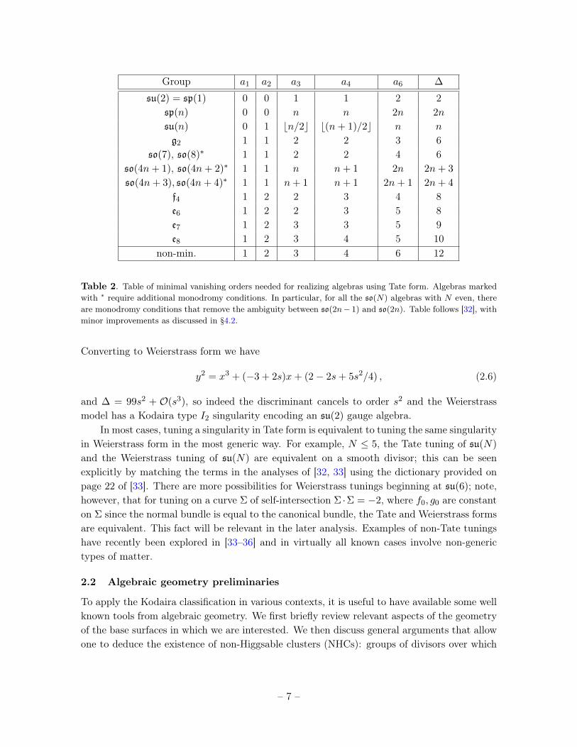
Table 2. Table of minimal vanishing orders needed for realizing algebras using Tate form. Algebras markedwith ∗ require additional monodromy conditions. In particular, for all the so(N) algebras with N even, thereare monodromy conditions that remove the ambiguity between so(2n− 1) and so(2n). Table follows [32], withminor improvements as discussed in §4.2.

Converting to Weierstrass form we have

y2 = x3 + (−3 + 2s)x+ (2− 2s+ 5s2/4) , (2.6)

and ∆ = 99s2 + O(s3), so indeed the discriminant cancels to order s2 and the Weierstrassmodel has a Kodaira type I2 singularity encoding an su(2) gauge algebra.

In most cases, tuning a singularity in Tate form is equivalent to tuning the same singularityin Weierstrass form in the most generic way. For example, N ≤ 5, the Tate tuning of su(N)

and the Weierstrass tuning of su(N) are equivalent on a smooth divisor; this can be seenexplicitly by matching the terms in the analyses of [32, 33] using the dictionary provided onpage 22 of [33]. There are more possibilities for Weierstrass tunings beginning at su(6); note,however, that for tuning on a curve Σ of self-intersection Σ ·Σ = −2, where f0, g0 are constanton Σ since the normal bundle is equal to the canonical bundle, the Tate and Weierstrass formsare equivalent. This fact will be relevant in the later analysis. Examples of non-Tate tuningshave recently been explored in [33–36] and in virtually all known cases involve non-generictypes of matter.

2.2 Algebraic geometry preliminaries

To apply the Kodaira classification in various contexts, it is useful to have available some wellknown tools from algebraic geometry. We first briefly review relevant aspects of the geometryof the base surfaces in which we are interested. We then discuss general arguments that allowone to deduce the existence of non-Higgsable clusters (NHCs): groups of divisors over which

– 7 –

even a generic fibration has a singularity that corresponds to a nontrivial gauge algebra. Thenwe introduce a few relevant aspects of toric geometry that allow one to explicitly execute agiven local tuned gauge algebra enhancement (increasing the Kodaira singularity) at the levelof coordinates; generally, such computations can be used to explicitly determine that a giventuned fibration is possible either locally or globally in a geometry with a local or global toricdescription. We primarily focus on local constructions in this paper, though in some situationsglobal analysis on a toric base is also relevant.

We are interested in complex surfaces B that can act as the base of an elliptically fiberedCalabi-Yau threefold. We thus focus on rational surfaces that can be realized by blowing upP2 or Fm,m ≤ 12 at a finite number of points. We review a few basic facts about such surfaces(for more details see e.g. [16]). Divisors in a complex surface are integer linear combinationsof irreducible algebraic curves on B. The set of homology classes of curves in B form asignature (1, T ) integer lattice Γ = H2(B,Z) = Z1+T where T = h1,1(B)−1. The intersectionform on Γ is unimodular, and for T 6= 1 can be written as diag (+1,−1,−1, . . . ,−1). (ForHirzebruch surfaces Fm with m even, the intersection form is the matrix ((01)(10)).) Thecanonical class K satisfies K ·K = 9 − T , and can be put into the form (3,−1,−1, . . . ,−1)

when the intersection form is diagonal as above, and in the form (2, 2) for even Hirzebruchsurfaces. The set of effective curves, which can be realized algebraically in B, form a conein the homology lattice. In F-theory, gauge groups can only be tuned on effective curves, sothese are the curves on which we focus attention. As an example of a set of allowed bases andtheir effective cones, the Hirzebruch surfaces Fm have a cone of effective curves generated bythe curves S, F where S · S = −m,S · F = 1, F · F = 0, and can support elliptic Calabi-Yauthreefolds when m = 0, . . . , 8, 12.

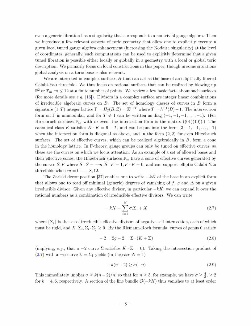
The Zariski decomposition [37] enables one to write −kK of the base in an explicit formthat allows one to read off minimal (generic) degrees of vanishing of f , g and ∆ on a givenirreducible divisor. Given any effective divisor, in particular −kK, we can expand it over therational numbers as a combination of irreducible effective divisors. We can write

− kK =

N∑i=1

σiΣi +X (2.7)

where {Σi} is the set of irreducible effective divisors of negative self-intersection, each of whichmust be rigid, and X ·Σi,Σi ·Σj ≥ 0. By the Riemann-Roch formula, curves of genus 0 satisfy

− 2 = 2g − 2 = Σ · (K + Σ) (2.8)

(implying, e.g., that a −2 curve Σ satisfies K · Σ = 0). Taking the intersection product of(2.7) with a −n curve Σ = Σ1 yields (in the case N = 1)

− k(n− 2) ≥ σ(−n) (2.9)

This immediately implies σ ≥ k(n− 2)/n, so that for n ≥ 3, for example, we have σ ≥ 43 , ≥ 2

for k = 4, 6, respectively. A section of the line bundle O(−kK) thus vanishes to at least order

– 8 –

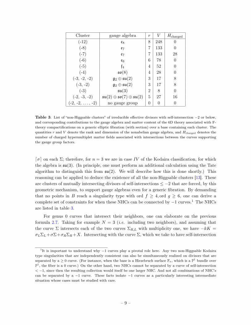
Cluster gauge algebra r V Hcharged

(-12) e8 8 248 0(-8) e7 7 133 0(-7) e7 7 133 28(-6) e6 6 78 0(-5) f4 4 52 0(-4) so(8) 4 28 0

(-3, -2, -2) g2 ⊕ su(2) 3 17 8(-3, -2) g2 ⊕ su(2) 3 17 8(-3) su(3) 2 8 0

(-2, -3, -2) su(2)⊕ so(7)⊕ su(2) 5 27 16(-2, -2, . . . , -2) no gauge group 0 0 0

Table 3. List of “non-Higgsable clusters” of irreducible effective divisors with self-intersection −2 or below,and corresponding contributions to the gauge algebra and matter content of the 6D theory associated with F-theory compactifications on a generic elliptic fibration (with section) over a base containing each cluster. Thequantities r and V denote the rank and dimension of the nonabelian gauge algebra, and Hcharged denotes thenumber of charged hypermultiplet matter fields associated with intersections between the curves supportingthe gauge group factors.

dσe on each Σ; therefore, for n = 3 we are in case IV of the Kodaira classification, for whichthe algebra is su(3). (In principle, one must perform an additional calculation using the Tatealgorithm to distinguish this from su(2). We will describe how this is done shortly.) Thisreasoning can be applied to deduce the existence of all the non-Higgsable clusters [13]. Theseare clusters of mutually intersecting divisors of self-intersections ≤ −2 that are forced, by thisgeometric mechanism, to support gauge algebras even for a generic fibration. By demandingthat no points in B reach a singularity type with ord f ≥ 4, ord g ≥ 6, one can derive acomplete set of constraints for when these NHCs can be connected by −1 curves.1 The NHCsare listed in table 3.

For genus 0 curves that intersect their neighbors, one can elaborate on the previousformula 2.7. Taking for example N = 3 (i.e. including two neighbors), and assuming thatthe curve Σ intersects each of the two curves ΣR,L with multiplicity one, we have −kK =

σLΣL+σΣ+σRΣR+X. Intersecting with the curve Σ, which we take to have self-intersection

1It is important to understand why −1 curves play a pivotal role here. Any two non-Higgsable Kodairatype singularities that are independently consistent can also be simultaneously realized on divisors that areseparated by a ≥ 0 curve. (For instance, when the base is a Hirzebruch surface Fn, which is a P1 bundle overP1, the fiber is a 0 curve.) On the other hand, two NHCs cannot be separated by a curve of self-intersection< −1, since then the resulting collection would itself be one larger NHC. And not all combinations of NHC’scan be separated by a −1 curve. These facts isolate −1 curves as a particularly interesting intermediatesituation whose cases must be studied with care.

– 9 –

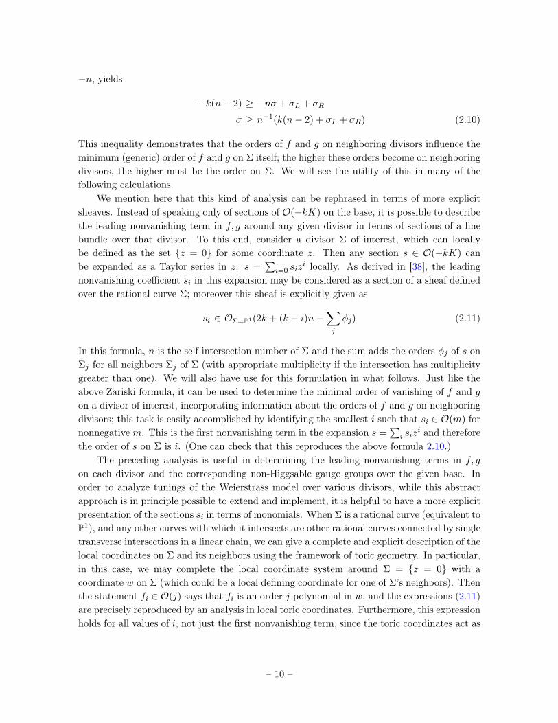
−n, yields

− k(n− 2) ≥ −nσ + σL + σR

σ ≥ n−1(k(n− 2) + σL + σR) (2.10)

This inequality demonstrates that the orders of f and g on neighboring divisors influence theminimum (generic) order of f and g on Σ itself; the higher these orders become on neighboringdivisors, the higher must be the order on Σ. We will see the utility of this in many of thefollowing calculations.

We mention here that this kind of analysis can be rephrased in terms of more explicitsheaves. Instead of speaking only of sections of O(−kK) on the base, it is possible to describethe leading nonvanishing term in f, g around any given divisor in terms of sections of a linebundle over that divisor. To this end, consider a divisor Σ of interest, which can locallybe defined as the set {z = 0} for some coordinate z. Then any section s ∈ O(−kK) canbe expanded as a Taylor series in z: s =

∑i=0 siz

i locally. As derived in [38], the leadingnonvanishing coefficient si in this expansion may be considered as a section of a sheaf definedover the rational curve Σ; moreover this sheaf is explicitly given as

si ∈ OΣ=P1(2k + (k − i)n−∑j

φj) (2.11)

In this formula, n is the self-intersection number of Σ and the sum adds the orders φj of s onΣj for all neighbors Σj of Σ (with appropriate multiplicity if the intersection has multiplicitygreater than one). We will also have use for this formulation in what follows. Just like theabove Zariski formula, it can be used to determine the minimal order of vanishing of f and gon a divisor of interest, incorporating information about the orders of f and g on neighboringdivisors; this task is easily accomplished by identifying the smallest i such that si ∈ O(m) fornonnegative m. This is the first nonvanishing term in the expansion s =

∑i siz

i and thereforethe order of s on Σ is i. (One can check that this reproduces the above formula 2.10.)

The preceding analysis is useful in determining the leading nonvanishing terms in f, g

on each divisor and the corresponding non-Higgsable gauge groups over the given base. Inorder to analyze tunings of the Weierstrass model over various divisors, while this abstractapproach is in principle possible to extend and implement, it is helpful to have a more explicitpresentation of the sections si in terms of monomials. When Σ is a rational curve (equivalent toP1), and any other curves with which it intersects are other rational curves connected by singletransverse intersections in a linear chain, we can give a complete and explicit description of thelocal coordinates on Σ and its neighbors using the framework of toric geometry. In particular,in this case, we may complete the local coordinate system around Σ = {z = 0} with acoordinate w on Σ (which could be a local defining coordinate for one of Σ’s neighbors). Thenthe statement fi ∈ O(j) says that fi is an order j polynomial in w, and the expressions (2.11)are precisely reproduced by an analysis in local toric coordinates. Furthermore, this expressionholds for all values of i, not just the first nonvanishing term, since the toric coordinates act as

– 10 –

global coordinates. In the following analysis, therefore, we focus on explicit local constructionsof tunings in the toric context, and freely use the language of toric geometry, which we nowreview briefly. Our use of toric geometry should always be understood as a convient wayto do calculations in local coordinates that are valid for genus zero curves intersecting withmultiplicity one. This kind of local analysis thus allows us to compute tunings on sets ofcurves that can be locally described torically, even if the full base geometry is not a toricsurface. When the base is itself a compact toric variety, toric coordinates can be used to coverthe full base and we can completely control the Weierstrass model in terms of monomials inthe toric language.

Here we recall some notions and notations from toric geometry; interested readers mayconsult excellent references such as [39] for more background. Most of the relevant conceptsare described in this context and in more detail in [14]. A toric variety can be describedby a fan, which for a two (complex) dimensional variety is characterized by a collection of rintegral vectors {vi}ri=1 in the lattice N = Z2, each of which represents a rational curve in atoric surface. We restrict attention to smooth toric varieties, where vi, vi+1 span a unit cell inthe lattice, associated with a 2D cone describing a point in the toric variety where a pair oflocal coordinates vanish. A rational curve of self-intersection −n satisfies nvj = vj−1 + vj+1.A compact toric variety also has a 2D cone connecting vr, v1. The principal formula we willborrow from toric geometry describes a basis of sections of line bundles over a toric variety,with fixed vanishing order on Dj ,

S(−kK)Dj ,nj = span({m ∈M | m · vi ≥ −n & m · vj = −k + nj}) (2.12)

The lhs denotes sections of −kK that vanish to order exactly nj on the particular divisor Dj

associated to vj , where −K = Dj +∑

i 6=j Di. (Taken together for all nj ≥ 0, this reproducesthe full collection of sections of O(−kK) without poles.) The additional constraints indexedby i correspond to conditions imposed from other toric rays. The rhs is the span of a basisof sections of −nK with the desired orders of vanishing. Finally, M denotes the dual latticeto N = Z2. In §4 and beyond, this formula is used frequently.

Note that unlike in [14], we are not necessarily performing a global analysis of toricmonomials. For a local analysis on a single divisor we only include the rays i = j± 1 adjacentto vj in the toric fan, while by increasing the number of rays we can include further adjacentdivisors in a linear chain, or by including all rays in the toric fan we can consider a globalanalysis on a toric base B.

2.3 6D supergravity

In the classification of 6D supergravity (SUGRA) vacua, one can bring to bear the additionaltool of anomaly cancellation, which turns out to be quite powerful. The Green-Schwarzmechanism is possible in 6D if and only if the anomaly polynomial factorizes, which canbe rephrased as a set of equations on various group theory quantities derived from simplefactors of the gauge group and their representations [5, 6, 40]. In fact, these equations are

– 11 –

restrictive enough to strongly constrain the set of possible 6D supergravity theories thatcan be realized from F-theory or any other approach [41, 9]. These relations can furthermoredetermine uniquely the matter content of the 6D theory in many cases. Vectors in the anomalypolynomial, which lie in the lattice of charged dyonic strings, map directly to certain divisorsinH2(B,Z), which for F-theory constructions enables computation of the low-energy spectrumof the theory and associated constraints purely in terms of easily computed quantities in thebase; this greatly simplifies the implementation of anomaly constraints in the F-theory context.The close connection between F-theory geometry and 6D supergravity theories is describedin, among other places, [7, 9, 10]. A detailed description of the low-energy supergravity actionfor 6D F-theory compactifications from the M-theory perspective is given in [42].

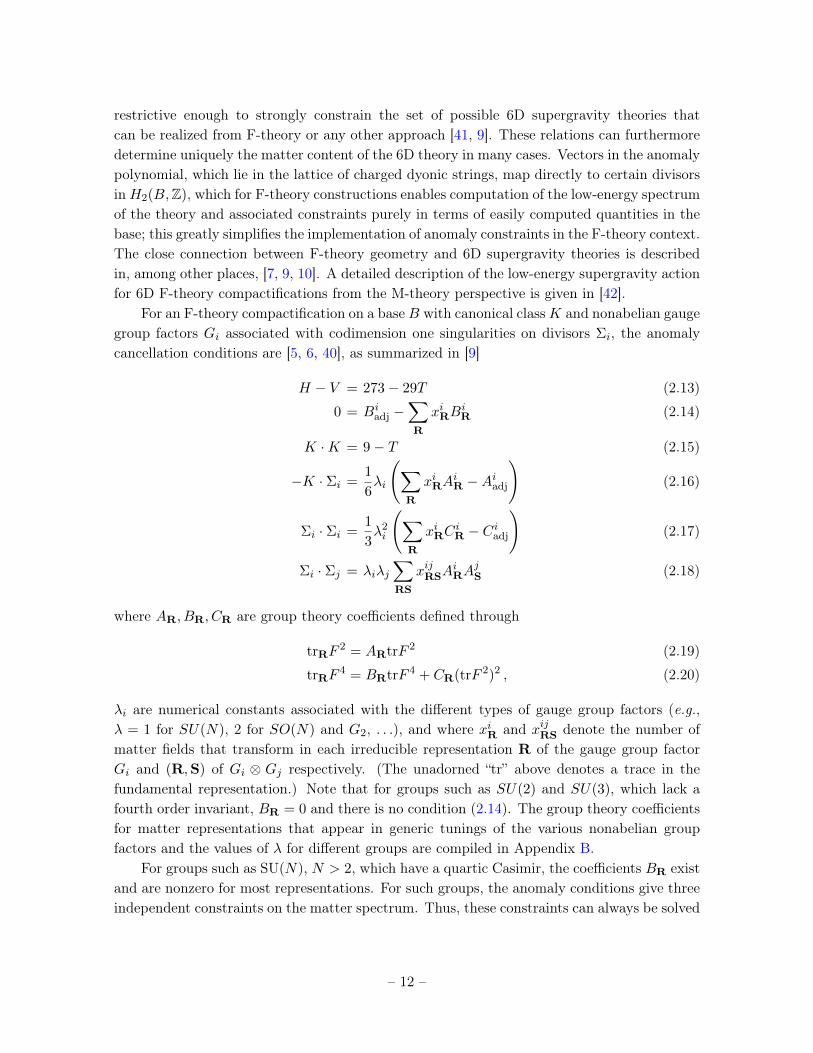
For an F-theory compactification on a base B with canonical classK and nonabelian gaugegroup factors Gi associated with codimension one singularities on divisors Σi, the anomalycancellation conditions are [5, 6, 40], as summarized in [9]

H − V = 273− 29T (2.13)

0 = Biadj −

∑R

xiRBiR (2.14)

K ·K = 9− T (2.15)

−K · Σi =1

6λi

(∑R

xiRAiR −Aiadj

)(2.16)

Σi · Σi =1

3λ2i

(∑R

xiRCiR − Ciadj

)(2.17)

Σi · Σj = λiλj∑RS

xijRSAiRA

jS (2.18)

where AR, BR, CR are group theory coefficients defined through

trRF2 = ARtrF 2 (2.19)

trRF4 = BRtrF 4 + CR(trF 2)2 , (2.20)

λi are numerical constants associated with the different types of gauge group factors (e.g.,λ = 1 for SU(N), 2 for SO(N) and G2, . . .), and where xiR and xijRS denote the number ofmatter fields that transform in each irreducible representation R of the gauge group factorGi and (R,S) of Gi ⊗ Gj respectively. (The unadorned “tr” above denotes a trace in thefundamental representation.) Note that for groups such as SU(2) and SU(3), which lack afourth order invariant, BR = 0 and there is no condition (2.14). The group theory coefficientsfor matter representations that appear in generic tunings of the various nonabelian groupfactors and the values of λ for different groups are compiled in Appendix B.

For groups such as SU(N), N > 2, which have a quartic Casimir, the coefficients BR existand are nonzero for most representations. For such groups, the anomaly conditions give threeindependent constraints on the matter spectrum. Thus, these constraints can always be solved

– 12 –

in terms of three basic representations. For each such group, generic F-theory tunings willproduce matter in a standard set of representations; for example, for SU(N), a generic tuninggives a combination of matter in the fundamental, two-index antisymmetric, and adjointrepresentations. For generic tunings, the number of adjoint representations is given by thegenus of the curve supporting the group. Any other, more exotic, representation will alwaysbe anomaly equivalent [9, 10] to a linear combination of the three basic representations. Weprimarily focus here on the generic representation content associated with minimal (Tate)tunings; exotic matter is discussed in §7. Note that many groups, particularly the exceptionalgroups and SU(2), have no quartic Casimir, and thus (2.14) identically vanishes. For thesegroups, there are only two independent anomaly constraints, and the generic matter contentconsists of only the fundamental and adjoint representations. This is discussed further in §4.4.

It is also worthwhile to comment briefly here on the purely gravitational anomaly condition(2.13). For a global F-theory model this constrains the number of moduli in the theory. Whilewe are primarily focused on local constraints here, it must be kept in mind that a globalmodel must satisfy (2.13), and in principle this constraint can produce additional limits onwhat may be tunable in a given Weierstrass model. In fact, in most cases it seems that thelimits on tuning can be determined purely from combinations of local constraints, so that thegravitational anomaly is generally automatically satisfied by an F-theory model when all localconstraints are satisfied; it is not, however, proven at this time that this must always be true.We focus on deriving local constraints in this paper, but occasionally reference the connectionto the global gravitational anomaly constraint.

In this paper we use the anomaly cancellation conditions to help constrain the possibilitiesfor F-theory tunings. We are also interested in exploring the “swampland” [24] of models thatappear consistent from known low-energy considerations but are not realized in F-theory.The 6D anomaly conditions as well as other constraints such as the sign of the gauge kineticterm can be used to strongly constrain 6D supergravity theories based on the consistencyof the low-energy theory. All consistent F-theory models should satisfy these constraints;otherwise F-theory would be an intrinsically inconsistent theory of quantum gravity. It hasbeen conjectured [23] that all consistent 6D N = 1 supergravity theories have a description instring theory. Given the close correspondence between the low-energy theory and the geometryof F-theory, and the fact that essentially all known consistent 6D SUGRA spectra that comefrom string theory can be realized in F-theory, it seems that F-theory may have the abilityto realize the full moduli space of consistent 6D supergravity theories. Thus, we highlightparticularly those cases where a given tuning seems consistent from low-energy considerationsbut does not have a known construction through an F-theory Weierstrass model.

2.4 6D SCFTs

In [18], Heckman, Morrison, and Vafa proposed a method of generating 6D SCFTs throughF-theory. Here we perform only a cursory review. One of the crucial ingredients in theclassification of [18], as in the classification of 6D supergravity theories, is the set of non-Higgsable clusters, which form basic units for composing 6D SCFTs.

– 13 –

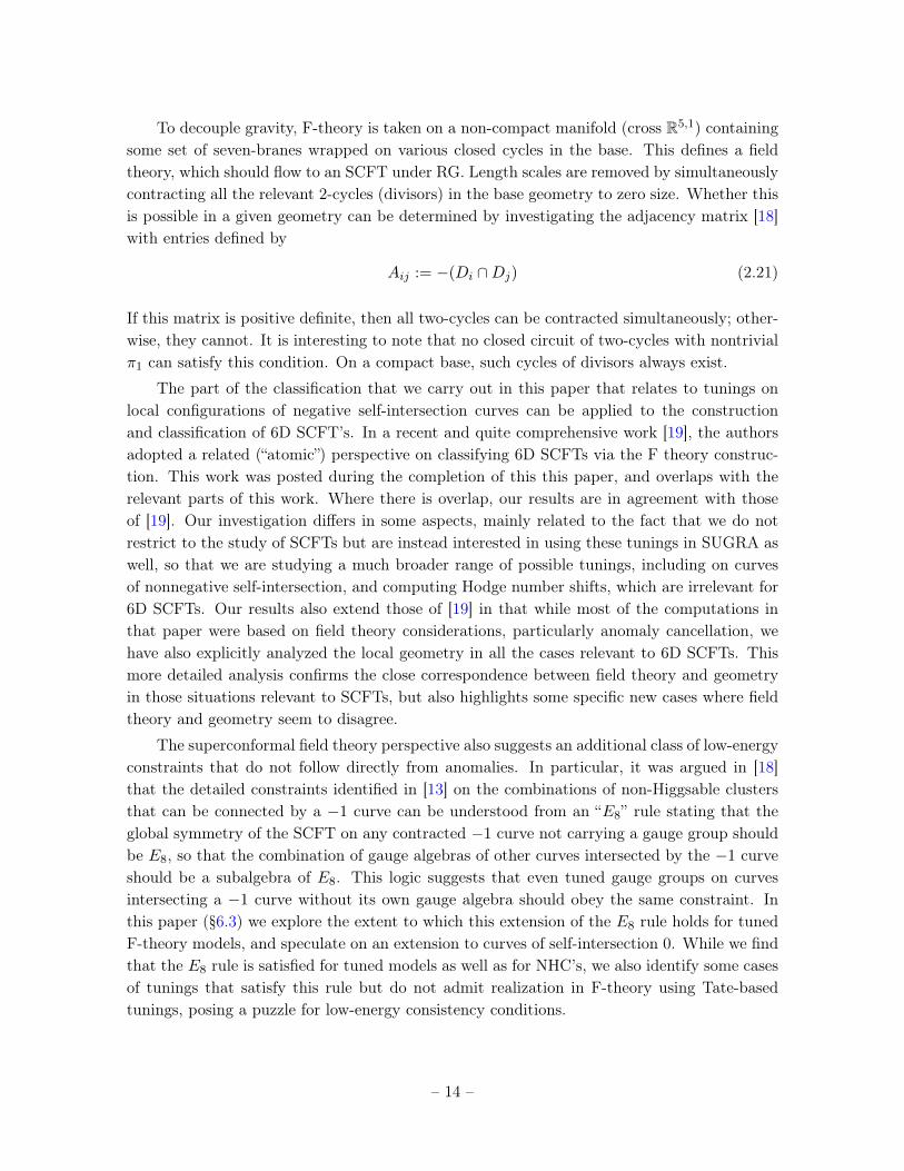
To decouple gravity, F-theory is taken on a non-compact manifold (cross R5,1) containingsome set of seven-branes wrapped on various closed cycles in the base. This defines a fieldtheory, which should flow to an SCFT under RG. Length scales are removed by simultaneouslycontracting all the relevant 2-cycles (divisors) in the base geometry to zero size. Whether thisis possible in a given geometry can be determined by investigating the adjacency matrix [18]with entries defined by

Aij := −(Di ∩Dj) (2.21)

If this matrix is positive definite, then all two-cycles can be contracted simultaneously; other-wise, they cannot. It is interesting to note that no closed circuit of two-cycles with nontrivialπ1 can satisfy this condition. On a compact base, such cycles of divisors always exist.

The part of the classification that we carry out in this paper that relates to tunings onlocal configurations of negative self-intersection curves can be applied to the constructionand classification of 6D SCFT’s. In a recent and quite comprehensive work [19], the authorsadopted a related (“atomic”) perspective on classifying 6D SCFTs via the F theory construc-tion. This work was posted during the completion of this this paper, and overlaps with therelevant parts of this work. Where there is overlap, our results are in agreement with thoseof [19]. Our investigation differs in some aspects, mainly related to the fact that we do notrestrict to the study of SCFTs but are instead interested in using these tunings in SUGRA aswell, so that we are studying a much broader range of possible tunings, including on curvesof nonnegative self-intersection, and computing Hodge number shifts, which are irrelevant for6D SCFTs. Our results also extend those of [19] in that while most of the computations inthat paper were based on field theory considerations, particularly anomaly cancellation, wehave also explicitly analyzed the local geometry in all the cases relevant to 6D SCFTs. Thismore detailed analysis confirms the close correspondence between field theory and geometryin those situations relevant to SCFTs, but also highlights some specific new cases where fieldtheory and geometry seem to disagree.

The superconformal field theory perspective also suggests an additional class of low-energyconstraints that do not follow directly from anomalies. In particular, it was argued in [18]that the detailed constraints identified in [13] on the combinations of non-Higgsable clustersthat can be connected by a −1 curve can be understood from an “E8” rule stating that theglobal symmetry of the SCFT on any contracted −1 curve not carrying a gauge group shouldbe E8, so that the combination of gauge algebras of other curves intersected by the −1 curveshould be a subalgebra of E8. This logic suggests that even tuned gauge groups on curvesintersecting a −1 curve without its own gauge algebra should obey the same constraint. Inthis paper (§6.3) we explore the extent to which this extension of the E8 rule holds for tunedF-theory models, and speculate on an extension to curves of self-intersection 0. While we findthat the E8 rule is satisfied for tuned models as well as for NHC’s, we also identify some casesof tunings that satisfy this rule but do not admit realization in F-theory using Tate-basedtunings, posing a puzzle for low-energy consistency conditions.

– 14 –

2.5 Calabi-Yau threefolds

One of the primary goals of this work is to use tunings as a means of exploring and classifyingthe space of elliptic Calabi-Yau threefolds. For any given elliptically fibered CY threefold Xwith a Weierstrass description over a given base B, the Hodge numbers of X can be read offfrom the form of the singularities and the corresponding data of the low-energy theory. Asuccinct description of the Hodge numbers of X can be given using the geometry-F-theorycorrespondence [2, 43, 8]

h1,1(X) = r + T + 2 (2.22)

h2,1(X) = H0 − 1 = 272 + V − 29T −Hcharged (2.23)

Here, T = h1,1(B) − 1 is the number of tensor multiplets in the 6D theory; r is the rank ofthe 6D gauge group and V is the number of vector multiplets in the 6D theory, while H0

and Hcharged refer to the number of 6D matter hypermultiplets that are neutral/charged withrespect to the Cartan subalgebra of the gauge group G. The relation (2.22) is essentially theShioda-Tate-Wazir formula [44]. The equality (2.23) follows from the gravitational anomalycancellation condition in 6D supergravity, H − V = 273− 29T, which corresponds to a topo-logical relation on the Calabi-Yau side that has been verified for most matter representationswith known nongeometric counterparts [7, 10]. The nonabelian part of the gauge group G

can be read off from the Kodaira types of the singularities in the elliptic fibration accordingto Table 1 (up to the discrete part, which does not affect the Hodge numbers and that we donot compute in detail here).

One use of these conditions is to compute the shifts in Hodge numbers for a given tuningof an enhanced gauge group on a given divisor or set of divisors. In many of the local situationswe consider here, we can directly compute the shift in the Hodge number h2,1 by determiningthe number of complex degrees of freedom (neutral scalar fields) that must be fixed in theWeierstrass model to realize the desired tuning. In other cases, where we do not have a localmodel, we can use (2.23) to compute h2,1 = H0−1 for a tuning based simply on the spectrumof the theory. Note that h1,1 follows simply from the gauge group and number of tensors,and does not depend upon the detailed matter spectrum. One subtlety is that in cases wherea tuned group can be broken to a smaller group without decreasing the rank, in particularfor G2 → SU(3), F4 → SO(8), and SO(2N + 1) → SO(2N), the charged fields under thelarger group that are uncharged under the smaller group of equal rank (and which do notcarry charge under any other group) still contribute to H0 and h2,1(X) as neutral multipletseven from the larger group as they are uncharged under the Cartan subalgebra [2]2, so thatthe Hodge numbers of the Calabi-Yau do not change in such a breaking. This phenomenonwill be treated in more detail elsewhere [45]. Note that a somewhat related situation in theN = 2 4D context is discussed in [46]. In these situations, in the low-energy theory theadditional vector fields in the larger nonabelian group cancel in the anomaly conditions withthe remaining charged fields in a charged multiplet; e.g., for g2 → su(3), a 7 → 3+ 3+1, the

2Thanks to Y. Wang for discussions on this point

– 15 –

1 acts as a neutral scalar, and the 3 + 3 cancel the additional six vector bosons in g2. Thisis relevant for many of the tunings discussed here. For clarity, when performing tunings wecompute explicitly the shift in the number of completely uncharged hypermultiplets Hu; inall cases except tunings of g2, f4, so(2N + 1) these correspond precisely to a shift in h2,1, whilein the case of g2, etc., the shift in h2,1 should be that associated with the equal-rank tuningwith su(3) etc. so the shift in Hodge numbers can be determined by considering the relatedmodel that is reached after a rank-preserving breaking. In the latter cases, where Hu 6= H0,

we denote the shift in Hu in brackets [∆Hu] to indicate this distinction.In cases where we have a global toric model, there is a direct relationship between H0 and

the number W of Weierstrass moduli given by the toric monomials in M that describe f, g.This relationship is given by

H0 = W − waut +N−2 , (2.24)

where N−2 is the number of −2 curves (on which the discriminant does not identically vanish),and waut is the number of automorphisms of the base, given by 2 for a generic base with notoric curves of self-intersection 0 or greater and adding n + 1 for every toric curve of self-intersection n ≥ 0. This formula allows us to directly compute the shift in h2,1 even in localtoric models by computing the local change in this quantity. There is one further additionalsubtlety [15], which is that certain combinations of −2 curves form degenerate elliptic curves;such configurations have an effective value of N−2 that must be decreased by 1. We encounterthis subtlety in §5.2.

One of the goals of this paper is to continue to develop a systematic set of tools forclassifying elliptic Calabi-Yau threefolds through F-theory. This might seem like the reverseof the logical order: to apply F theory, one needs to know about (elliptically fibered) Calabi-Yaus. But there are still many unanswered questions about Calabi-Yau threefolds in general;for example, it is still unknown whether there are a finite or infinite number of topologicaltypes of non-elliptic Calabi-Yau threefolds. Some evidence suggests [47, 43, 48, 49, 17, 50] that,particularly for large Hodge numbers, a large fraction of Calabi-Yau threefolds and fourfoldsthat can be realized using known construction methods are elliptically fibered. Since thenumber of elliptic Calabi-Yau threefolds is finite this suggests that the number of Calabi-Yauthreefolds may in general be finite, and that understanding and classifying elliptic Calabi-Yau threefolds may give insights into the general structure of Calabi-Yau manifolds. As anexample of how the methods developed here can be used in classification of elliptic Calabi-Yau threefolds, in §10.1 we identify several large classes of known Calabi-Yau threefolds inthe Kreuzer-Skarke database as tunings of generic elliptic fibrations over allowed bases.

In the context of classification of Calabi-Yau threefolds, there is an additional point thatshould be brought out. Our classification is essentially one of Weierstrass models, whichcontain various Kodaira singularity types. While any elliptic Calabi-Yau threefold has acorresponding Weierstrass model, the Weierstrass models for any theory with a nontrivialKodaira singularity type, corresponding to a nonabelian gauge group in the low-energy 6DF-theory model, have singular total spaces. The singularities in the total space must be

– 16 –

resolved to get a smooth Calabi-Yau threefold. This resolution at the level of codimension onesingularities maps essentially to Kodaira’s original classification of singularities. Resolutionsat codimension two, however, are much more subtle, and in many cases a singular Weierstrassmodel can have multiple distinct resolutions at codimension two, corresponding to differentCalabi-Yau threefolds with the same Hodge numbers but different triple intersection numbers.There has been quite a bit of work in recent years on these codimension two resolutions in theF-theory context [33, 51–56], but there is as yet no complete and systematic description of whatelliptic Calabi-Yau threefolds can be related to a given Weierstrass model. For the purposesof classifying 6D F-theory models this distinction is irrelevant, but it would be important inany systematic attempt to completely classify all smooth elliptic Calabi-Yau threefolds.

3 Outline of results

The following three sections represent the core of this work. In them, we present and derivea set of fairly simple rules that can be used to determine which gauge symmetries and matterrepresentations are allowed, given the local geometric data of a set of one or more intersectingdivisors within a complex base surface appropriate for F-theory. For each tuning over the localdivisor geometry, we compare the constraints given from low-energy consistency conditions tothe possibility of an explicit F-theory construction. Before diving into details, we pause todelineate our results and outline our methods and strategy.

The setting of our analysis is 6D F-theory, i.e. F-theory compactified on a Calabi-Yauthreefold that results from an elliptic fibration with section over a two (complex)-dimensionalbase manifold B. We focus on local combinations of effective divisors (curves) in B. We focusparticularly on smooth rational (genus 0) curves that intersect pairwise in a single point. Thesecases are particularly amenable to study: we can analyze them locally using toric methods,they are the only divisor combinations needed to tune elliptic Calabi-Yau threefolds that ariseas hypersurfaces in toric varieties as studied in [57], and they are the only configurationsneeded for analyzing 6D SCFTs. For these combinations of curves, we carry out a thoroughanalysis using both the field theory (anomaly) approach and a local geometric approach forexplicit construction of Weierstrass and/or Tate models. In these cases we can confirm that,with a few notable exceptions that we highlight, the anomaly constraints match perfectly withthe set of configurations that is allowed in a local Weierstrass model. In addition to thesecases where we have both local geometry and field theory control of the configuration, wealso consider more briefly more general configurations needed to complete the classification oftunings over a generic base, including higher genus curves (§4.4), exotic matter representationsthat can arise for non-generic tunings on smooth curves or tunings on singular curves (§7), andtuning of abelian gauge symmetries, which requires global structure through the Mordell-Weilgroup (§8).

The results of our analysis could be applied in a variety of ways. Most simply, they providea toolkit for easily developing a broad range of examples of 6D F-theory supergravity modelsand corresponding elliptic Calabi-Yau threefolds and/or 6D SCFTs; given a base geometry

– 17 –

one can construct a set of tuned models with any particular desired properties subject toconstraints imposed by the base geometry. More generally, these results can be used in asystematic classification of 6D supergravity models or SCFTs. A complete list of toric basesthat support 6D supergravity models was computed in [14]. The results presented here inprinciple give the local information needed to construct all possible tunings on toric curvesover these bases, which could be used to compare with the Kreuzer-Skarke database [58] togive an interpretation of many of the constructions in that large dataset in terms of ellipticfibrations and to identify those examples of Calabi-Yau threefold that are not ellipticallyfibered. The broader set of constraints described here for more general tunings in principlegives the basic components needed for a systematic classification of all tunings, includingon non-toric curves over generic bases. Combined with the systematic classification of bases[16], this provides a framework for the complete classification of all Weierstrass models forelliptic Calabi-Yau threefolds. A more detailed description of how such an algorithm wouldproceed is given in §9. Note that in this more general context, and even to some extent inthe more restricted toric context, our rules really only provide a superset of the set of allowedtunings. The local rules that we provide, even when supported by local explicit Weierstrassconstructions, must be checked for a global tuning for compatibility by explicit constructionof a global Weierstrass model that satisfies all the conditions needed for the tuning. While weexpect that at least in the toric context, local rules are essentially adequate for determiningthe set of allowed tunings, in a more global context this is less clear. For toric bases, there isan explicit description of the Weierstrass model in terms of monomials [14], so that, at leastfor tuning over toric divisors in toric bases, the technology for producing a global Weierstrassmodel is available. For more general bases, or tunings over non-toric curves, a concise andeffective approach for tuning Weierstrass models is not at present known to the authors.

Within this setting, we summarize the results of the following sections. These results canbe summarized in terms of the following data: given a base-independent local collection ofdivisors {Di} with given genera and self- and mutual intersections, we determine a list L[{Di}]of the possible gauge symmetries over these divisors, along with the matter representationsand shifts in the Hodge numbers (∆h1,1,∆h2,1) between the generic and tuned models.

• Section 4 analyzes tunings L[Σ] for isolated divisors Σ with −12 ≤ Σ ·Σ. Curves of self-intersection below −12 cannot arise in valid F-theory bases, and no tuning is possibleover any curve with self intersection below −6. Local models are used to describe alltunings on genus 0 curves, and tunings on higher genus curves are constrained throughanomalies.

• Section 5 determines L[C] for NHCs C that consist of strings of multiple intersecting di-visors. Explicitly, these are the multi-curve NHCs (−3,−2,−2), (−2,−3,−2), (−3,−2),and clusters of −2 curves of arbitrary size. (There are in practice bounds on the sizeand complexity of such −2 clusters that can appear F-theory SUGRA bases, some ofwhich we discuss here). Local toric models are used for the NHCs with −3 curves, and

– 18 –

a simple “convexity” feature is used to classify tunings over −2 clusters, the validity ofwhich is checked in Tate models in §6.

• Section 6 analyzes multiple intersecting curves beyond the NHCs. We show that thereare only five combinations of gauge algebras (or families thereof) that can be tuned onintersecting pairs of divisors, and analyze the constraints on these combinations usinglocal (largely Tate) methods. We also consider constraints on tunings of multiple branesintersecting a single brane, both when the single brane carries a gauge group and whenit does not. The latter case includes the “E8 rule” [18] governing what gauge groups canbe realized on divisors that intersect a −1 curve, which we generalize to include tunings,and a similar but weaker rule for curves of self-intersection zero.

• Section 7 gives some further rules that apply for tuning exotic matter representationswith a finer tuning that leaves the gauge group (and h1,1(X)) invariant while modifyingthe matter content. The underlying F-theory geometry and corresponding mathematicalstructure of non-Tate Weierstrass models is only partially understood at this point sothis set of results may be incomplete.

• Section 8 gives a guide to tuning abelian gauge factors over a given base. While muchis known and we can make some clear statements about tunings and constraints, this isalso a rapidly evolving area of research and this set of results may also be improved byfurther progress in understanding such models.

4 Classification I: isolated curves

In this section we consider all possible tunings of enhanced groups on individual divisors in thebase. In general, a divisor in the base is a curve Σ of genus g and self-intersection Σ · Σ = n.In this section we concentrate on generic tunings of a given gauge group, which means thatthe curve Σ is generally smooth, and supports only certain generic types of matter. Forexample, for su(N) a generic Weierstrass tuning on a genus 0 curve will give matter only inthe fundamental (N) and antisymmetric (N(N − 1)/2) representations; when the genus g isnonzero, there are also g adjoint (N2 − 1) matter fields. Further tunings that keep the gaugegroup fixed but enhance the matter content are discussed in §7.

For each type of curve and gauge group we consider both anomaly constraints and theexplicit tuning through the Weierstrass model of the gauge group. We focus primarily onrational (genus 0) curves. For individual rational curves we find an almost perfect matchingbetween those tunings that are allowed by anomaly cancellation and what can be realizedexplicitly in F-theory Weierstrass models. For curves of negative self-intersection that can oc-cur in non-Higgsable clusters, and for exceptional algebras tuned on arbitrary rational curves,we compute the Hodge shifts explicitly in Weierstrass models and confirm the match withanomaly conditions. For curves of self-intersection −2 and above supporting the classical

– 19 –

series su(N), sp(N), and so(N), we use the Tate method to construct Weierstrass modelsexplicitly, and anomaly cancellation to predict the Hodge number shifts.

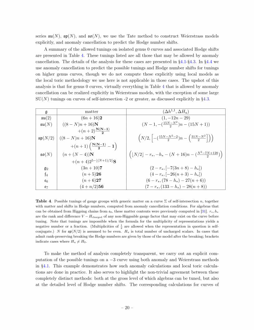
A summary of the allowed tunings on isolated genus 0 curves and associated Hodge shiftsare presented in Table 4. These tunings listed are all those that may be allowed by anomalycancellation. The details of the analysis for these cases are presented in §4.1-§4.3. In §4.4 weuse anomaly cancellation to predict the possible tunings and Hodge number shifts for tuningson higher genus curves, though we do not compute these explicitly using local models asthe local toric methodology we use here is not applicable in those cases. The upshot of thisanalysis is that for genus 0 curves, virtually everything in Table 4 that is allowed by anomalycancellation can be realized explicitly in Weierstrass models, with the exception of some largeSU(N) tunings on curves of self-intersection -2 or greater, as discussed explicitly in §4.3.

g matter (∆h1,1,∆Hu)

su(2) (6n+ 16)2 (1,−12n− 29)

su(N) ((8−N)n+ 16)N (N − 1,−(15N−N2

2 )n− (15N + 1))

+(n+ 2)N(N−1)2

sp(N/2) ((8−N)n+ 16)N(N/2,

[−(15N−N2−2

2 )n−(

31N−N2

2

]))+(n+ 1)

(N(N−1)

2 − 1)

so(N) (n+ (N − 4))N(bN/2c − r∗,−h∗ − (N + 16)n− (N

2−7N+1282 )

)+(n+ 4)25−b(N+1)/2cS

g2 (3n+ 10)7 (2− r∗, [−7(3n+ 8)− h∗])f4 (n+ 5)26 (4− r∗, [−26(n+ 3)− h∗])e6 (n+ 6)27 (6− r∗, (78− h∗)− 27(n+ 6))

e7 (4 + n/2)56 (7− r∗, (133− h∗)− 28(n+ 8))

Table 4. Possible tunings of gauge groups with generic matter on a curve Σ of self-intersection n, togetherwith matter and shifts in Hodge numbers, computed from anomaly cancellation conditions. For algebras thatcan be obtained from Higgsing chains from e8, these matter contents were previously computed in [31]. r∗, h∗

are the rank and difference V −Hcharged of any non-Higgsable gauge factor that may exist on the curve beforetuning. Note that tunings are impossible when the formula for the multiplicity of representations yields anegative number or a fraction. (Multiplicities of 1

2are allowed when the representation in question is self-

conjugate.) N for sp(N/2) is assumed to be even. Hu is total number of uncharged scalars. In cases thatadmit rank-preserving breaking the Hodge numbers are given by those of the model after the breaking; bracketsindicate cases where Hu 6= H0.

To make the method of analysis completely transparent, we carry out an explicit com-putation of the possible tunings on a −3 curve using both anomaly and Weierstrass methodsin §4.1. This example demonstrates how such anomaly calculations and local toric calcula-tions are done in practice. It also serves to highlight the non-trivial agreement between thesecompletely distinct methods: both at the gross level of which algebras can be tuned, but alsoat the detailed level of Hodge number shifts. The corresponding calculations for curves of

– 20 –

self-intersection −4 and below, as well as the multiple-curve non-Higgsable clusters, can befound in Appendix C.

Before proceeding with the example calculation, we should note that the core of this sec-tion’s results, Table 4, can be found to a large extent in a corresponding table in [31]. Ourversion differs from that in [31] in two respects: we include algebras that are not subalgebrasof e8, and we also include shifts in Hodge numbers that result from implementing these tun-ings. This extra information is essential in order to use these tunings as an organizationaltool to search through the set of elliptically fibered threefolds. Finally, our analysis of localWeierstrass models allows us to determine that virtually all of these configurations that areallowed by anomaly analysis are actually realizable locally in F-theory, with some specificpossible exceptions that we highlight.

Following the extended example of tunings on a −3 curve, we give a general analysis oftunings on curves of self-intersection −2 and above; these cases can be uniformly describedin a single framework. In these sections and in the Appendix, we discuss all possible tuningsexcept for so(N), because these tunings are particularly delicate. so(N) tunings are separatelydescribed in §4.2.

4.1 Extended example: tunings on a −3 curve

Let us begin with an extended example that will illustrate many of the features of the followingcomputations. On an isolated −3 curve, the minimal gauge algebra is su(3), which can beenlarged as

g = su(3) −→ g2 −→ so(7) −→ so(8) −→ f4 −→ e6 −→ e7

(f, g) = (2, 2) −→ { (2, 3) } −→ { (3, 4) } −→ (3, 5)(4.1)

The middle three and subsequent two gauge algebras are distinguished by monodromy of thesingularity, as per the Kodaira classification; we will describe this in detail below. These tunedalgebras and their associated matter all fall in a Higgsing chain from e7. The complete set oftunings a priori allowed on a −3 curve also includes so(N) for 8 < N ≤ 12, but these will bediscussed in the following section.

4.1.1 Spectrum and Hodge shifts from anomaly cancellation

First we will perform an anomaly calculation; then we will discuss a local toric model (essen-tially F3 with the +3 curve removed) on which we can implement these tunings. A tabulationof the relevant anomaly coefficients AR, BR, CR and λ values is given in Appendix B Taking

– 21 –

the “C” condition, we find:

Σ · Σ =λ2

3

(∑R

CR − CAdj

)

−3 =1

3

(∑R

CR − 9

)0 =

∑R

CR (4.2)

Since all coefficients CR > 0 for su(3) (which follows from the definition of CR and the absenceof a quartic Casimir), this implies that no matter transforms under this gauge group; there isonly the vector multiplet in the adjoint 8. This in turn implies that the presence of this gaugealgebra contributes to the quantity H0 (2.23) by an amount h∗ = V − Hcharged and r∗ = 2

(this algebra’s rank) to h1,1. Since the gauge algebra su(3) (with no matter) corresponds tothe generic elliptic fibration over a −3 curve (i.e., −3 is an NHC), we conclude that all shiftsbetween the generic case and a tuned case in the Hodge numbers (∆h1,1,∆h2,1 ∼ ∆H0) =

(∆r,∆(V −Hcharged) must be calculated as (∆h1,1,∆H0) = (rtuned−2, Vtuned−Hcharged,tuned−8), as denoted in Table 4.

With this most generic case in mind, let us calculate the corresponding quantities for g2.Assuming only fundamental matter3, with a multiplicity Nf , anomaly calculation gives

Σ · Σ =λ2

3

(∑R

CR − CAdj

)

−3 =4

3

(Nf

4− 5

2

)Nf = 1 (4.3)

The contribution to Hu is (recall that the adjoint of g2 has dimension 14 and the fundamentalhas dimension 7):

∆Hu = 14− 7− 8 = +7− 8 = [−1] (4.4)

In other words, implementing this tuning decreases Hu by one in comparison to the genericcase. Note that, as mentioned in §2.5, one of the charged scalars in the 7 of g2 will reallyact as a neutral scalar for purposes of computing h2,1(X), since it can be used to break thegauge group without reducing rank. We continue to treat this scalar as charged, withoutcontributing to Hu, here and in the rest of the paper, but this caveat should be kept in mindfor all g2, f4 and so(2n+ 1) tunings, and is indicated by the notation [−1].

3This is the generic matter type expected for g2. More generally, other C coefficients are ≥ 5/2 and thereforethe presence of even one hypermultiplet in one of these non-fundamental representations makes it impossibleto satisfy the C condition on any negative self-intersection curve.

– 22 –

For so(7), CAdj = 3, which implies [41] that the only relevant representations on negativeself-intersection curves are 7f and 8s. Since Cf = 0 and Cs = 3

8 , we have

Σ · Σ =λ

3

(∑R

CR − CAdj

)

−3 =4

3

(Ns

3

8− 3

)Ns = 2 (4.5)

One can then use the “A” condition to demonstrate4 that Nf = 0:

K · Σ =λ

6

(Aadj −

∑R

AR

)

1 =1

3(5−Ns −Nf )

3 = (5− 2−Nf )

Nf = 0 (4.6)

With knowledge of the representation content in hand, we can compute the change in Hu:

∆Hu = ∆(V −H) = 21− 2× 8− 8 = −3 . (4.7)

Note that the absence of fundamental matter in this case means that there is no rank-preserving breaking so(7) → g2, so that the shift in Hu = H0 is not denoted in brackets.A similar calculation for so(8) yields Ns = 2, Nf = 1, hence

∆Hu = ∆(V −H) = 28− 3× 8− 8 = +4− 8 = −4 (4.8)

Proceeding to f4, we find again that only fundamental matter is possible on a (−3)-curve, and

Σ · Σ =λ

3

(∑R

CR − CAdj

)

−3 =62

3

(Nf

12− 5

12

)−3 = Nf − 5

Nf = 2 (4.9)

Recalling that the dimensions of the fundamental and adjoint are 26 and 52, respectively, wefind

∆Hu = 52− 2× 26− 8 = [−8] (4.10)

4In calculating K · Σ, we use (K + Σ) · Σ = 2g − 2 = −2 for a genus 0 curve (topologically P1).

– 23 –

For e6, we find

Σ · Σ =λ2

3

(∑R

CR − CAdj

)

−3 =62

3

(Nf

12− 1

2

)Nf = 3 (4.11)

Given that the dimensions of fundamental and adjoint are 27 and 78, respectively,

∆Hu = 78− 3× 27− 8 = −3− 8 = −11 (4.12)

Enhancing finally to e7, we find

Σ · Σ =122

3

(N

24− 1

6

)−3 = 2(N − 4)

N =5

2(4.13)

which is possible because the fundamental 56 of e7 is self-conjugate, and hence admits a half-hypermultiplet in six dimensions. This contributes to Hu in the amount +133 − 5

256 = −7,i.e. represents a shift of −4 subsequent to tuning an e6, or in total ∆Hu = −15 from thegeneric case of su(3).

These calculations can be summarized simply as:

g su(3) g2 so(7) so(8) f4 e6 e7

∆Hu 0 [−1] −3 −4 [−8] −11 −15(4.14)

4.1.2 Spectrum and Hodge shifts from local geometry

Now we would like to explain this from a more direct geometric viewpoint. We will find that wemust be careful to implement the most generic tuning, which (when we consider monodromy)will not always be obtained simply by setting monomial coefficients to zero. We use a localmodel that can be considered a convenient way to visualize the monomials in f and g (inlocal coordinates); alternately, our local models are simply concrete ways of generating thefull set of monomials consistent with equations 2.11. Torically, the self-intersection numberof any toric divisor Σ ↔ vi corresponding to vi in the fan can be determined by the formulavi−1 + vi+1 = −(Σ · Σ)vi. Therefore, a linear chain of k rational curves with any specifiedself-intersection numbers may be realized by a toric fan with k + 2 rays, which correspondsto a non-compact toric variety. In this example, we need three rays (corresponding to the −3

curve and its neighbors). Without loss of generality, we take this fan to be (3,−1), (1, 0), (0, 1).Using the methods of section 2, we find that the monomials of −nK are determined to liewithin (or on the boundary of) a wedge determined by the conditions: x ≥ −n, y ≥ −n, andy ≤ n+ 3x. The first condition is automatically satisfied when the latter two are.

– 24 –

●

●

●

●

●

●

●

●

●

●

●

●

●

●

●

●

●

●

●

●

●

●

●

●

●

●

●

●

●

●

●

●

●

●

●

●

●

●

●

●

●

-4 -3 -2 -1 1 2 3

-4

-3

-2

-1

1

2

3

● ●

●

●

●

●

●

●

●

●

●

●

●

●

●

●

●

●

●

●

●

●

●

●

●

●

●

●

●

●

●

●

●

●

●

●

●

●

●

●

●

●

●

●

●

●

●

●

●

●

●

●

●

●

●

●

●

●

●

●

●

●

●

●

●

●

●

●

●

●

■■

-6 -5 -4 -3 -2 -1 1 2 3

-6

-5

-4

-3

-2

-1

1

2

3

4

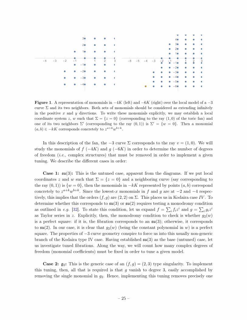
Figure 1. A representation of monomials in −4K (left) and −6K (right) over the local model of a −3

curve Σ and its two neighbors. Both sets of monomials should be considered as extending infinitelyin the positive x and y directions. To write these monomials explicitly, we may establish a localcoordinate system z, w such that Σ = {z = 0} (corresponding to the ray (1, 0) of the toric fan) andone of its two neighbors Σ′ (corresponding to the ray (0, 1)) is Σ′ = {w = 0}. Then a monomial(a, b) ∈ −kK corresponds concretely to za+kwb+k.

In this description of the fan, the −3 curve Σ corresponds to the ray v = (1, 0). We willstudy the monomials of f (−4K) and g (−6K) in order to determine the number of degreesof freedom (i.e., complex structures) that must be removed in order to implement a giventuning. We describe the different cases in order:

Case 1: su(3): This is the untuned case, apparent from the diagrams. If we put localcoordinates z and w such that Σ = {z = 0} and a neighboring curve (say corresponding tothe ray (0, 1)) is {w = 0}, then the monomials in −kK represented by points (a, b) correspondconcretely to za+kwb+k. Since the lowest-x monomials in f and g are at −2 and −4 respec-tively, this implies that the orders (f, g) are (2, 2) on Σ. This places us in Kodaira case IV . Todetermine whether this corresponds to su(3) or su(2) requires testing a monodromy conditionas outlined in e.g. [32]. To state this condition, let us expand f =

∑i fiz

i and g =∑

i gizi

as Taylor series in z. Explicitly, then, the monodromy condition to check is whether g2(w)

is a perfect square: if it is, the fibration corresponds to an su(3); otherwise, it correspondsto su(2). In our case, it is clear that g2(w) (being the constant polynomial in w) is a perfectsquare. The properties of −3 curve geometry conspire to force us into this usually non-genericbranch of the Kodaira type IV case. Having established su(3) as the base (untuned) case, letus investigate tuned fibrations. Along the way, we will count how many complex degrees offreedom (monomial coefficients) must be fixed in order to tune a given model.

Case 2: g2: This is the generic case of an (f, g) = (2, 3) type singularity. To implementthis tuning, then, all that is required is that g vanish to degree 3, easily accomplished byremoving the single monomial in g2. Hence, implementing this tuning removes precisely one

– 25 –

degree of freedom∆Hu = [−1]

as we had concluded earlier using anomaly calculations.

Case 3: so(7): We now encounter a more subtle issue of counting. The monodromyconditions that distinguish the three gauge algebras that can accompany a (2, 3) singularityare specified by the factorization properties of the polynomial

x3 + f2(w)x+ g3(w) , (4.15)

x3 +Ax+B (generic) ⇒ g2

(x−A)(x2 +Ax+B) ⇒ so(7)

(x−A)(x−B)(x+ (A+B)) ⇒ so(8) (4.16)

The coefficients here are chosen in order to ensure that no quadratic term appears in the totalcubic polynomial. To obtain the second condition (so(7)), we proceed by writing explicitly

x3 + (f2,0 + f2,1w + f2,2w2)x+ (g3,0 + g3,1w + g3,2w

2 + g3,3w3) . (4.17)

This expression uses explicit knowledge of the monomials. Recalling that the order in w

of a monomial (a, b) in −4K is b + 4, we may read off that the only monomials of f2 are{w0, w1, w2}. Similarly, the only monomials available for g3 are {w0, w1, w2, w3}. The sevencoefficients above must then be tuned to enforce the appropriate factorization. Expandingthe factorized version of the cubic (in x) polynomial, it is clear that we must impose that thecoefficient of x be given by B − A2 and that of x0 given by −AB. This can be minimallyaccomplished by setting to zero the coefficients c and g above. More generally, A and B mustbe respectively linear and quadratic, with 5 independent degrees of freedom. This representsa loss of two additional degrees of freedom (besides the first, which represented tuning fromsu(3) to g2). Hence

∆Hu = −3 (4.18)

again in accordance with the anomaly results.

Case 4: so(8): Consulting the list above, to achieve so(8), we must completely factorizethe polynomial. Expanding yields the constraints

a+ bw + cw2 = −A2 −AB −B2

d+ ew + fw2 + gw3 = AB(A+B) (4.19)

This requires that now both B and A must be linear in w, so we can for example simply setthe f coefficient to zero as well. This removes an additional 1 degree of freedom (beyond thepreviously removed three) leading to

∆Hu = −4 (4.20)

– 26 –

as expected from anomaly results.

Case 5: f4: To tune to the f4/e6 case, we must enhance the degrees of vanishing of f andg to (3, 4), which requires that we eliminate all (a, b) ∈ −4K with b ≤ −2 and (c, d) ∈ −6K

with d ≤ −3. The generic such tuning is an f4 algebra. Inspecting the monomial figure, wefind that from the initial (untuned) scenario, this requires us to eliminate the leftmost columnof f (3 monomials) and the leftmost two columns of g (1 + 4 monomials), so that in total

∆Hu = [−8] (4.21)

as expected from anomaly results.

Case 6: e6: In this case, the monodromy condition is whether g4 is a perfect square.Counting up from the left (as before), the available monomials are {w0, w1, ..., w6}. We canmake this polynomial of degree 6 into a square by restricting it to be of the form

g4(w) = (α+ βw + δw2 + εw3)2 , (4.22)

which clearly preserves 4 of the 7 original degrees of freedom. This counting indicates that(as expected) we lose 3 more degrees of freedom in tuning from f4 to e6, for a total change of

∆Hu = −11 (4.23)

from the original (untuned) su(3). Note that this minimal tuning cannot be reached by simplysetting to 0 three of the coefficients in g4.

Case 7: e7: Enhancing finally to e7 requires enhancing the degrees of vanishing of (f, g)

to (3, 5). Up to this point, we have already enhanced to (3, 4), so it remains only to eliminatethe remaining 7 monomials of g4, yielding a shift in Hu of −7 in comparison to a tuning of f4,or a shift of −4 subsequent to tuning e6, in accordance with anomaly calculations.

We thus have found that explicit computation of Weierstrass models with monomialsconfirms that all tunings compatible with anomaly cancellation on a −3 curve can be realizedin F-theory, with the proper number of degrees of freedom tuned in each case.

4.2 Special case: tuning so(N > 8)

We have not so far explored the tuning of so(N) with N > 8, i.e. a Kodaira type I∗m>0

singularity. Such gauge algebras are non-generic in two ways: 1) they require a vanishing of∆ to order greater than the minimum min{2 ord(f), 3 ord(g)}, and 2) even and odd so(N)

are distinguished by a subtle monodromy condition [59]. Due to these complications, wehave reserved the treatment of these tunings to this section. The results to follow are almostprecisely in accord with Table 4, by applying the rule that a tuning is not allowed when theformula for the multiplicity of any of its representations becomes negative or fractional (withfractions of 1

2 allowed for real representations). However, for clarity, we explicitly list theallowed tunings for −2, −3, and −4 curves in Table 5.

– 27 –

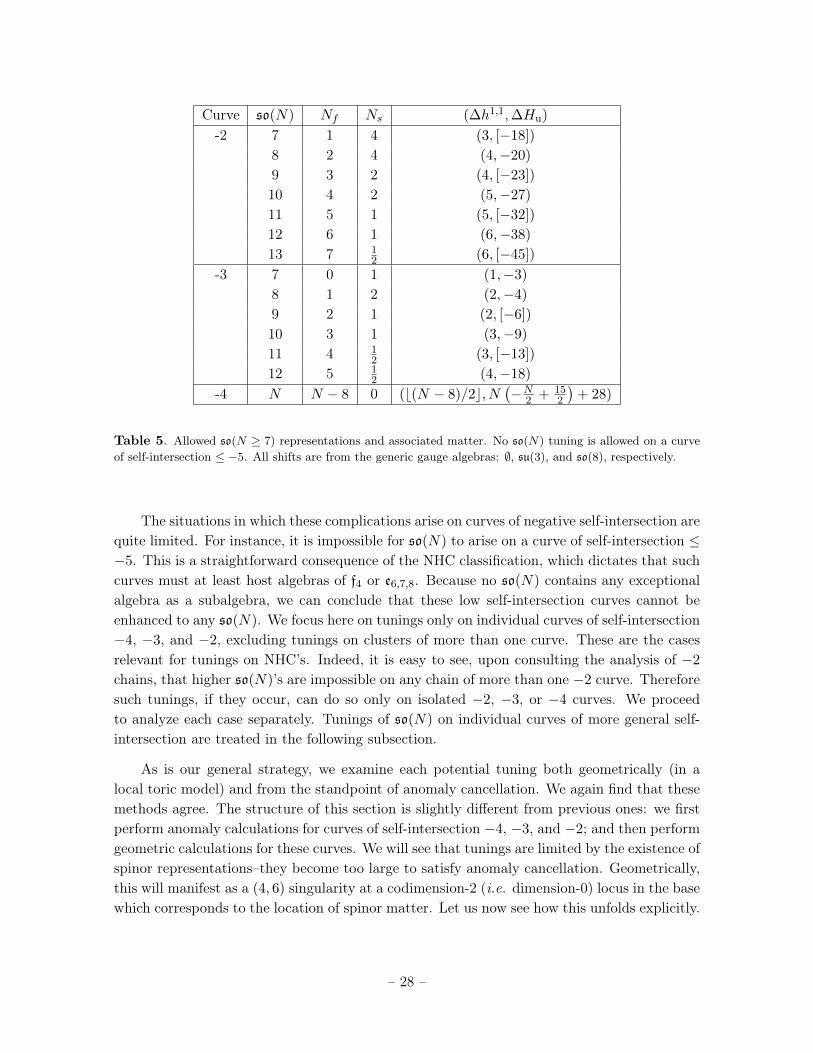
Curve so(N) Nf Ns (∆h1,1,∆Hu)

-2 7 1 4 (3, [−18])

8 2 4 (4,−20)

9 3 2 (4, [−23])

10 4 2 (5,−27)

11 5 1 (5, [−32])

12 6 1 (6,−38)

13 7 12 (6, [−45])

-3 7 0 1 (1,−3)

8 1 2 (2,−4)

9 2 1 (2, [−6])

10 3 1 (3,−9)

11 4 12 (3, [−13])

12 5 12 (4,−18)

-4 N N − 8 0 (b(N − 8)/2c, N(−N

2 + 152

)+ 28)

Table 5. Allowed so(N ≥ 7) representations and associated matter. No so(N) tuning is allowed on a curveof self-intersection ≤ −5. All shifts are from the generic gauge algebras: ∅, su(3), and so(8), respectively.

The situations in which these complications arise on curves of negative self-intersection arequite limited. For instance, it is impossible for so(N) to arise on a curve of self-intersection ≤−5. This is a straightforward consequence of the NHC classification, which dictates that suchcurves must at least host algebras of f4 or e6,7,8. Because no so(N) contains any exceptionalalgebra as a subalgebra, we can conclude that these low self-intersection curves cannot beenhanced to any so(N). We focus here on tunings only on individual curves of self-intersection−4, −3, and −2, excluding tunings on clusters of more than one curve. These are the casesrelevant for tunings on NHC’s. Indeed, it is easy to see, upon consulting the analysis of −2

chains, that higher so(N)’s are impossible on any chain of more than one −2 curve. Thereforesuch tunings, if they occur, can do so only on isolated −2, −3, or −4 curves. We proceedto analyze each case separately. Tunings of so(N) on individual curves of more general self-intersection are treated in the following subsection.

As is our general strategy, we examine each potential tuning both geometrically (in alocal toric model) and from the standpoint of anomaly cancellation. We again find that thesemethods agree. The structure of this section is slightly different from previous ones: we firstperform anomaly calculations for curves of self-intersection −4, −3, and −2; and then performgeometric calculations for these curves. We will see that tunings are limited by the existence ofspinor representations–they become too large to satisfy anomaly cancellation. Geometrically,this will manifest as a (4, 6) singularity at a codimension-2 (i.e. dimension-0) locus in the basewhich corresponds to the location of spinor matter. Let us now see how this unfolds explicitly.

– 28 –

4.2.1 Spectrum and Hodge shifts from anomaly cancellation

The anomaly calculation proceeds simply, but reveals an intricate pattern of spinors dependingupon the curve self-intersection, matching e.g. [31]. First notice that the adjoint represen-tation has Cadj = 3, and therefore the C condition can be satisfied only for representationswith C ≤ 3. (There are no representations with negative C.) Given λ = 2 for so(N), the Ccondition takes the form

Σ · Σ =4

3

(∑R

CR − 3

)(4.24)

Indeed, since we consider only curves with Σ ·Σ < 0, the only representations that can cancelthe −3 are those with C < 3. As discussed in [41], the only such representations are the fun-damental (C = 0) and the spinor (for N ≤ 13). Given that the fundamental representationdoes not contribute at all to this condition, this equation uniquely fixes the number of spinorrepresentations on a given curve. The results are summarized in table 5. It is important inimplementing these conditions to recall that the 32 and 64 dimensional spinor representations(of so(11/12) and so(13)) are both self-conjugate. Therefore, half-hypermultiplets can trans-form in these representations. These hypers are counted with multiplicity 1

2 ; if they were tobe counted with multiplicity 1, anomaly cancellation for so(11/12) would be impossible ona −3 curve and anomaly cancellation for so(13) would be impossible on a −2 curve. As anexample, on a −3 curve, the C condition reads −9

4 + 3 = 34 = NsCs. For N = 9, 10, Cs = 3

4 ,so there is one spinor rep. For N = 11, 12, Cs = 3

2 and therefore a half-hyper spinor rep isrequired. Above this, we can see that Cs = 3, and even the smallest amount of spinor matter,a half-hyper, can no longer satisfy anomaly cancellation. As spinors were the only candidatesto satisfy these conditions in the first place, we can decisively state that so(N) tunings withN > 12 are forbidden on −3 curves.

As to the fundamental representations, their numbers can be determined from the Acondition

K · Σ =1

3

(∑R

AR −Aadj

)(4.25)

Using As = 2b(N+1)/2c−4, Aadj = N − 2, and Af = 1, we can easily solve for Nf . Forinstance, on a −3 curve, we have already determined that there is 1 spinor hyper for so(9/10)

and 12 for so(11/12). Since the left hand side of the condition is K · Σ = −1, we obtain

−3 = Nf+NsAs−(N−2). As an example, for so(9) on a−3 curve, this givesNf = 7−2−3 = 2.For so(10), the only change is that Aadj = 10−2 = 8 increases by one, henceNf = 3. Similarly,forN = 11, 12, although only a half-hyper transforms in the spin representation, the coefficientAs doubles in comparison to the previous cases. Thus again, the only numerical change is thatAadj increases by one as N increases; Nf = 5, 6 for so(11/12). This one example of tuningson a −3 curve illustrates the general pattern of matter representations on all three curvesconsidered; further calculations are entirely analogous and are therefore omitted.

– 29 –

One final remark is in order: we found that so(13) was the largest so(N) that anomaliesallow on a −2 curve and so(12) was the highest allowed on a −3 curve. One might expect thispattern to continue, with e.g. so(10) the highest possible tuning on a −4 curve. But, at thisvery lowest self-intersection curve before such tunings become impossible, they regain renewedvigor: all so(N)’s are tunable on a −4 curve. It is straightforward to verify that the matterin table 5 for a −4 curve satisfies anomaly cancellation. The reason there is no restriction issimply that it was the spin representations that led to a problem before, and on a −4 curve,there are no spin represenations: all matter is in the fundamentals.

4.2.2 Spectrum and Hodge shifts from local geometry

Now we check the predictions from anomaly cancellation by constructing, where possible, localmodels for the allowed so(N) tunings and showing how the disallowed tunings fail. These localcalculations are subtler than others we have so far encountered. Namely, we must impose anon-generic vanishing of ord(∆) > min{3 ord(f), 2 ord(g)}. Moreover, there are two distinctmonodromy conditions distinguishing so(8+2m) from so(7+2m) in the I∗m Kodaira case, onecondition each for n even and odd. These conditions are clearly stated in [10, 32]. For ourpurposes, instead of using these results directly, we note that the monodromy conditions canbe summarized succinctly as follows. To be in the generic Kodaira case I∗m, i.e. so(7 + 2m),requires that ∆ vanish to order 6 +m. However ∆6+m must not vanish; otherwise we wouldbe in the next highest Kodaira case. All monodromy conditions for I∗m can be summarized asthe requirement that ∆6+m be a perfect square. When this is the case, the resulting gaugealgebra is enhanced so(7 + 2m) −→ so(8 + 2m).

For our local models, we use the fan {(0, 1), (1, 0), (n,−1)}, where n is (negative) theself-intersection number of the middle curve Σ represented by the vector (1, 0) and assumesthe values 2, 3, 4. Because a −3 curve is the simplest example that captures the complexityof these tunings, we begin with it, moving then to −2 and finally −4 curves.

On a −3 curve, we will be able to tune up to but not including an so(13). Let us seehow this is possible. We have already seen how an so(8) may be tuned, so let us investigatethe first new case: so(9), i.e. the generic I∗1 singularity. To implement this tuning, we simplyrequire

∆6 ∝ f32 + g2

3 = 0 (4.26)

In the above we suppress the coeffients of the separate terms (4 and 27, respectively) as theywill play no role in determining whether this quantity can be set to zero and (if this is possible)how many degrees of freedom must be fixed to do so. In implementing this condition, we mustkeep in mind that the orders of f and g must remain 2 and 3, respectively. It is clear thatsuch a tuning (on a smooth divisor) will be possible iff f2 is a perfect square and g3 is a perfectcube. Indeed, expanding in a local defining coordinate w for the curve represented by (0, 1),we see that fn ∼ w3n−4 and gn ∼ w3n−3, which we will use repeatedly. In particular, f2 ∼ w2

– 30 –

and g3 ∼ w3,5 whence this condition can be satisfied if f2 ∝ φ2, g3 ∝ φ3 for an arbitrarylinear term φ = a + bw. Note that for cancellation between these terms, the two coefficientsa and b are arbitrary but fixed between f and g, and moreoever, once an overall coefficientfor φ2 is chosen for f2, this fixes the overall coefficient of φ3. Hence there are 2 degreesof freedom remaining, whereas we started with 3 + 4 = 7 in arbitrary quadratic and cubicpolynomials. Therefore, we lose 5 degrees of freedom in this tuning, in precise accordance withthe change ∆Hu predicted from the matter determined by anomaly cancellation. (NB: Thischange is counted from g2, the generic (2, 3) singularity.) Comparing with the known changeof ∆Hu = −3 in tuning so(8) from g2, we see that this tuning represents a loss of 2 additionaldegrees of freedom. (Or, from the generic non-Higgsable algebra su(3), we have ∆Hu = −6).To reassure ourselves that this indeed works, we recall the anomaly calculation: su(3) has nohypers, only a vector in the adjoint, so its contribution to Hu (in the terms V −Hcharged) is+8. For so(9), we have both vectors and hypermultiplets, so the contribution to V −Hcharged

is +36− 1 · 16− 2 · 9 = +2, a loss of 6 degrees of freedom.To tune an so(10) requires implementing a mondromy condition: g4 + 1

3φf3 must be aperfect square [32]. This is indeed possible, and since g4 ∼ w6, we lose 3 degrees of freedom inrequiring that it take the form (∼ w3)2. Again, we have a match with anomaly cancellation.

To tune an so(11) we now require ∆7 = 0, namely

0 = ∆7 ∝ f3f22 + g3g4

= f3φ4 + φ3g4 (4.27)

Now this will be possible with g4 ∝ φf3, which consumes all the degrees of freedom of g4, i.e.all 7 (or the 4 that remain after tuning an so(10)); again, we have agreement with anomalycancellation calculations.

To tune an so(12), we now impose the more complicated monodromy condition that

µ = 4φ(g5 +1

3φf4)− f2

3 (4.28)

be a perfect square. This is also possible. We have 10 degrees of freedom in g5 ∼ w9 and 6 inf3 ∼ w5. By requiring g5 ∝ φg5, g5 ∼ w8 and f3 ∝ φf3, f3 ∼ w4, we can factor out φ2 fromµ; we can then tune g5 so that µ/φ2 is a perfect square, so that we satisfy the monodromycondition (4.28). This fixes 1+4 = 5 degrees of freedom, consistent with anomaly cancellation.

What goes wrong at the crucial case so(13)? To implement this tuning, we must set tozero ∆8:

0 = ∆8 ∝ f23 f2 + f2

2 f4 + g3g5 + g24

= f23φ

2 + φ4f4 + φ3g5 (4.29)

We combined the first and last terms upon recalling that g4 ∝ φf3. For this quantity to bezero, φ must divide f2

3 , which implies in this case that φ divides f3 because φ cannot be a5The notation ∼ wn will be used throughout this section to denote a polynomial of degree n in w with

arbitrary coefficients.

– 31 –

perfect square. This leads to an unacceptable singularity on the curve Cφ = {φ = 0}! Thisarises because, now, φ2|f2 and φ|f3, so that f vanishes to order 4 on Cφ. Meanwhile, we havealready found that φ3|g3, and now φ2|g4 and φ|g5. This leads directly to a (4, 6) singularityon Cφ.

On a −2 curve, the story is similar but slightly more complicated: we can tune up to butnot including so(14), in agreement with anomaly cancellation.6 Geometrically, we will see thatthe so(14) tuning fails for reasons similar to but slightly different from the failures we havepreviously encountered. To begin investigating these tunings, note that on this geometry, fn,gn ∝ w2n. On an isolated −2 curve, we have f2 ∼ w4, g3 ∼ w6, which implies that an I∗1 canbe tuned by taking φ = a+bw+cw2 to be an arbitrary quadratic. In the process, 5+7−3 = 9

degrees of freedom are fixed. This is to be interpreted as a change from g2, the generic (2, 3)

gauge algebra; or since so(8) can be tuned from g2 by fixing 6 degrees of freedom, this is achange of 3 additional degrees of freedom from so(8), consistent with anomaly cancellationcalculations. (Recall that anomaly cancellation predicts ∆Hu = −14, −20, −23 for g2, so(8),and so(9), respectively.) We can continue the analysis exactly as before, and no subtletiesarise in counting degrees of freedom. Let us jump, then, to the case of so(13), the generic I∗3singularity. Again we must require

0 = ∆8 ∝ f23φ

2 + φ4f4 + φ3g5 (4.30)

but in this case, φ is quadratic and can therefore be chosen to be a perfect square. Hence wecan satisfy the required condition φ|f2

3 while also maintaining φ - f3. Let us denote ψ2 = φ.Making this choice, namely fixing a quadratic to be the square of a linear function eliminatesone degree of freedom. Also, factoring f3 = ψf3, for generic degree 5 f3, we lose one moredegree of freedom. Finally, setting g5 = f2

3 + φf4 fixes all 11 degrees of freedom of g5 ∼ w10.This completes the required cancellation, fixing 1 + 1 + 11 = 13 degrees of freedom in theprocess. This matches with the shift from so(11) expected from anomaly cancellation.

It is not possible to tune so(14). The appropriate monodromy condition is to require that∆9 be a perfect square.

∆9 = ψ3

(−1

2f3

3 − 18ψ2f3f4 + 108ψ3(g6 − f5ψ

2))

(4.31)

As the f33 term has lowest order (in ψ), it cannot be cancelled by any other term unless ψ|f3

3 ,hence ψ|f3. But now ψ|g5 = f2

3 +ψ2f4, and one can check that our previous constraints havelikewise made all lower order terms in f and g divisible by ψ to sufficiently high order that a(4, 6) singularity at {φ = 0} is inevitable, and we conclude that so(14) cannot be tuned on a−2 curve. This conclusion was also reached in [64] based on the analysis of [10], and matchesthe expectation from anomaly cancellation.

On a −4 curve, the discussion is completely analogous, save for one crucial difference:f2, g3 ∼ z0 are constants, therefore φ is a constant. It is always true that a constant divides

6Thanks to Nikhil Raghuram and Yuji Tachikawa for illuminating discussions on this point.

– 32 –

higher order terms in ∆, and this condition therefore places no restrictions on the tunings. Onan isolated −4 curve, there is no apparent restriction on tuning so(N)’s. In SUGRA models,of course, large N will eventually cease to be tunable because h2,1 is finite and there willnot be sufficiently many complex degrees of freedom to implement the tuning. Such failuresresult from global properties of the base. From an anomaly cancellation standpoint, thisfailure eventually results from an inability to satisfy gravitational anomaly cancellation. Aswe discuss in §6.3, a local bound on N can also be imposed by other curves of non-positiveself intersection that intersect a −4 curve supporting an so(N), though such bounds are notfully understood in the low-energy theory. In SCFT’s, there is no reason to expect that theseries of so(N) tunings will ever terminate at any N .

4.3 Tuning on rational curves of self-intersection n ≥ −2

In this section we consider the possible tunings on an isolated curve of self-intersection n ≥ −2.For such curves, it is straightforward to use anomaly analysis along the lines of the precedingsection to confirm that in general the generic matter spectrum is that given by Table 4 for eachof the groups listed. Since in some cases the set of possible tunings is unbounded given onlylocal constraints, a case-by-case analysis is impossible. Fortunately, beginning at n = −2, wecan systematically organize the computation easily as a function of n. For the exceptional Liealgebras (e, f, g) we can check that the tunings are possible using Weierstrass, and explicitlycheck the Hodge numbers. For the classical Lie algebras (sp, su) we use Tate form. Forso(N) the analysis closely parallels that of the previous section, and we compare the Tate andWeierstrass perspectives.

4.3.1 Tuning exceptional algebras on n ≥ −2 curves

For simplicity we begin with −1 curves, then generalize. From the local toric analysis, wehave an expansion of f, g in polynomials fk, gk in a local coordinate w, where deg (fk) = 4+k,deg (gk) = 6 + k. The number of independent monomials in f0, f1, . . . and g0, g1, . . . are thus5, 6, . . . and 7, 8, . . . respectively.

To tune an e7 on the −1 curve, we must set f0 = f1 = f2 = g0 = · · · g4 = 0. This canclearly be done by setting 63 independent monomials to vanish. Thus, we can tune the e7 andwe confirm the Hodge number shift in Table 4. A similar computation allows us to tune f4by the same tuning but leaving g4 generic (11 monomials), giving the correct Hodge shift of52. For e6 we have the monodromy condition that g4 is a perfect square, so we get the correctshift by 57. Finally, for g2 we leave f2, g3 generic (7+10 = 17 monomials), for a correct Hodgeshift of 35. We have the usual caveat regarding the f4 and g2 and rank-preserving breaking.

We can generalize this analysis by noting that on a curve of self-intersection n ≥ −2, thelocal expansion gives

deg(fk) = 8 + n(4− k), deg(gk) = 12 + n(6− k) . (4.32)

Tuning any of the exceptional algebras on any such curve then is possible, since the degree isnonnegative for k ≤ 4, 6 for f, g respectively. The number of Weierstrass monomials that must

– 33 –

be tuned can easily be computed in each case and checked to match with Table 4. In thiscomparison it is important to recall from (2.24) that each −2 curve contributes an additionalneutral scalar field, while each curve of self-intersection n ≥ 0 contributes n+1 to the numberof automorphisms, effectively removing Weierstrass moduli from the neutral scalar count. Forexample, for e7 the number of monomials tuned is

((9 + 4n) + · · ·+ (9 + 2n)) + ((13 + 6n) + · · · (13 + 2n)) = 92 + 29n . (4.33)

The number of neutral scalars removed by this tuning is then

92 + 29n− (n+ 1) = 91 + 28n , (4.34)

in perfect agreement with the last line of Table 4. The shifts for the other exceptional groupscan similarly be computed to match the anomaly prediction.

4.3.2 Tuning su(N) and sp(N) on n ≥ −2 curves

We now consider the classical Lie algebras, beginning with su(N). These tunings are moresubtle for several reasons. First, the tunings involve a cancellation in ∆ that is not automati-cally imposed by vanishing of lower order terms in f, g so the computation of such tunings ismore algebraically involved. Second, these tunings can involve terms of arbitrarily high orderin ∆, f, g, and can be cut off when higher order terms do not exist in f, g, even in a purelylocal analysis.

To illustrate the first issue consider the tuning of su(2) on a −1 curve. The analysis ofthe general su(N) tuning through Weierstrass was considered in [33]. For su(2), this tuninginvolves setting f0 = −3φ2, g0 = 2φ3 to guarantee the cancellation of ∆0, and then solving thecondition ∆1 = 0 for g1. On a −1 curve this amounts to replacing the 5+7+8 = 20 monomialsin f0, f1, g1 with 3 monomials in a quadratic φ. The shift inHu is therefore by 17, in agreementwith Table 4. As N increases, the explicit tuning of the Weierstrass model in this way becomesincreasingly complicated. For N ≥ 6, there are multiple branches, including those withnon-generic matter contents, even for smooth curves; we return to this in §7. A systematicprocedure for tuning su(N) for arbitrary N through explicit algebraic manipulations of theWeierstrass model is not known. Thus, in these cases rather than attempting to explicitlycompute the Weierstrass model to all orders we simply use the Tate approach described in§2.1.

Already from Table 4, we can see that as n increases, the bound of allowed values on Nso that the number of fundamental representations is nonnegative decreases. We then wish todetermine which values of N can be realized using the Tate description and compare with thisbound from anomalies. For n = −2,−1, 0, there is no bound on N from anomalies. To analyzethe Tate forms, we determine the degrees of the coefficients in an expansion ai =

∑k ai(k)z

k

to be, in parallel to (4.32),deg(ai(k)) = 2i+ n(i− k) . (4.35)

– 34 –

To tune su(N), we must tune in Tate form a2 to vanish to order 1, a3 to vanish to order bn/2c,etc.. This can clearly be done for any N on n = −2,−1, 0 curves, so there is no problem withtuning any of these groups, consistent with the absence of a constraint from anomalies.

Now, however, consider for example a curve of self-intersection +1. From anomalies wesee that the number of fundamental matter representations is 16 + (8−N)n = 24−N , whichbecomes negative for N > 24. So we want to check which values of N ≤ 24 admit a Tatetuning of su(N). For n = 1, the maximum degree possible of the ai’s is

deg(a1, a2, a3, a4, a6) = (3, 6, 9, 12, 18). (4.36)

For each ai, this is the largest value of k such that (4.35) is nonnegative. To tune a Tatesu(24), we need the a’s to vanish to orders (0, 1, 12, 12, 24). This can be achieved by settinga3 = a6 = 0 and leaving arbitrary the largest terms in a4 (i.e., a4(12)). So we can tune throughTate an su(24). Tuning a higher su(N) would require the vanishing also of a4 to all orders,which would produce a singular Weierstrass model with ∆ = 0 everywhere, consistent withthe anomaly constraint. This is not the end of the story, however. To tune a Tate su(23)

requires the a’s to vanish to orders (0, 1, 11, 12, 23). But since there is no order 11 term in a3

or order 23 term in a6, this drives the Tate model automatically to su(24). Thus, there is noTate tuning of su(23) on a +1 curve. Similarly, there is no Tate tuning of su(21), althoughsu(22) may be tuned; and su(19) can also be tuned without obstruction. Precisely this samepattern was encountered in [33] when an attempt was made to tune these groups directly inthe Weierstrass model over a +1 curve, although in that context a particular simplificationwas made and there was no complete proof that there was no more complicated construction ofthese algebras. The upshot, however, is that on a curve of self-intersection +1, there is a slightdiscrepancy between the anomaly constraints and what we have been able to explicitly tunethrough Tate or Weierstrass. We have an almost exact agreement, but the gauge algebrassu(21) and su(23) lie in the “swampland” of models that seem consistent from low-energyconditions but cannot at this time be realized in any known version of string theory.

We can perform a similar analysis for the su(N) groups on other curves of positive selfintersection; the results of this analysis are tabulated in Table 6. Several other curve types havesimilarly missing su(N) groups in the Tate analysis. For +2,+3 curves it is impossible to tunesu(15), su(13) respectively using the Tate form, an explicit attempt to construct Weierstrassmodels showed a similar obstruction (with some simplifying assumptions made) in [8]. Itis interesting to note that in most of the cases where the Tate analysis does not provide ansu(N−1) but does allow for tuning an algebra su(N), the su(N) theory always has either zeroor one hypermultiplets in the fundamentalN representation, so that there is no direct Higgsingto su(N −1). One might think that in the two cases (n = 1, N = 22 and n = 7, N = 10) thereshould be two fundamentals, so that the theory might be Higgsable to the missing model.In the su(22) case, for example however, this tuning also forces7 an additional su(2) to arisein some cases on a curve that intersects Σ; this would absorb the two fundamentals into a

7Thanks to Nikhil Raghuram for pointing this out.

– 35 –

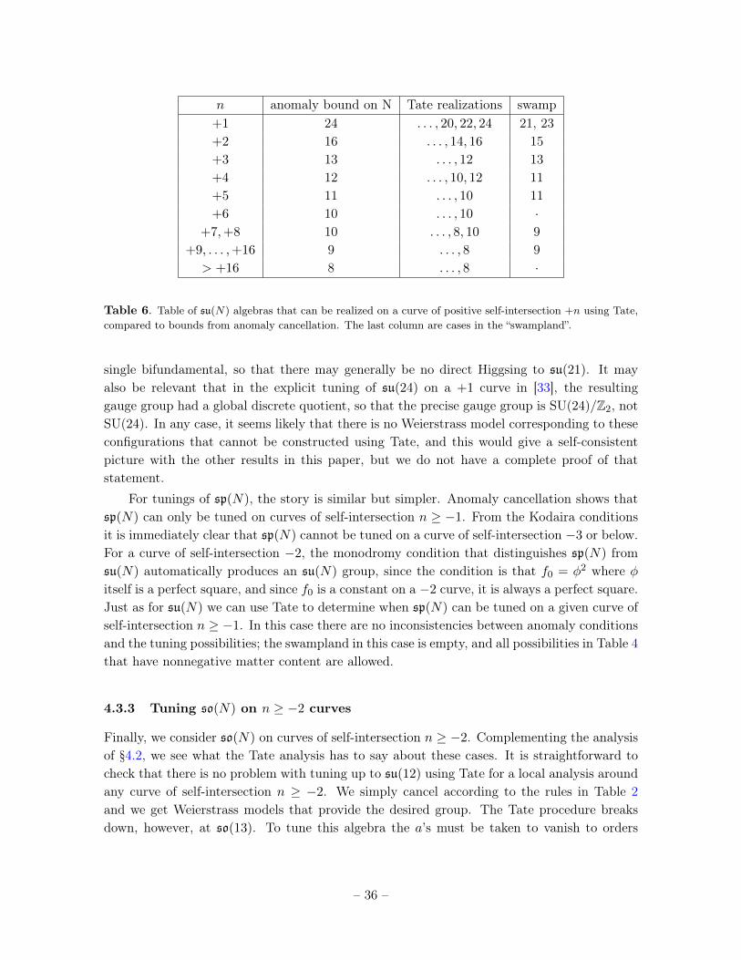
n anomaly bound on N Tate realizations swamp+1 24 . . . , 20, 22, 24 21, 23+2 16 . . . , 14, 16 15+3 13 . . . , 12 13+4 12 . . . , 10, 12 11+5 11 . . . , 10 11+6 10 . . . , 10 ·

+7,+8 10 . . . , 8, 10 9+9, . . . ,+16 9 . . . , 8 9> +16 8 . . . , 8 ·

Table 6. Table of su(N) algebras that can be realized on a curve of positive self-intersection +n using Tate,compared to bounds from anomaly cancellation. The last column are cases in the “swampland”.

single bifundamental, so that there may generally be no direct Higgsing to su(21). It mayalso be relevant that in the explicit tuning of su(24) on a +1 curve in [33], the resultinggauge group had a global discrete quotient, so that the precise gauge group is SU(24)/Z2, notSU(24). In any case, it seems likely that there is no Weierstrass model corresponding to theseconfigurations that cannot be constructed using Tate, and this would give a self-consistentpicture with the other results in this paper, but we do not have a complete proof of thatstatement.

For tunings of sp(N), the story is similar but simpler. Anomaly cancellation shows thatsp(N) can only be tuned on curves of self-intersection n ≥ −1. From the Kodaira conditionsit is immediately clear that sp(N) cannot be tuned on a curve of self-intersection −3 or below.For a curve of self-intersection −2, the monodromy condition that distinguishes sp(N) fromsu(N) automatically produces an su(N) group, since the condition is that f0 = φ2 where φitself is a perfect square, and since f0 is a constant on a −2 curve, it is always a perfect square.Just as for su(N) we can use Tate to determine when sp(N) can be tuned on a given curve ofself-intersection n ≥ −1. In this case there are no inconsistencies between anomaly conditionsand the tuning possibilities; the swampland in this case is empty, and all possibilities in Table 4that have nonnegative matter content are allowed.

4.3.3 Tuning so(N) on n ≥ −2 curves

Finally, we consider so(N) on curves of self-intersection n ≥ −2. Complementing the analysisof §4.2, we see what the Tate analysis has to say about these cases. It is straightforward tocheck that there is no problem with tuning up to su(12) using Tate for a local analysis aroundany curve of self-intersection n ≥ −2. We simply cancel according to the rules in Table 2and we get Weierstrass models that provide the desired group. The Tate procedure breaksdown, however, at so(13). To tune this algebra the a’s must be taken to vanish to orders

– 36 –

(1, 1, 3, 4, 6). Taking the Tate form

y2 + za1yx+ z3a3y = x3 + za2x2 + z4a4x+ z6a6 , (4.37)

and converting to Weierstrass form we find that a2 divides all coefficients in f and g up tof4, g6. This is the φ that played a key role in the analysis of §4.2. Unless φ = a2 is a constant,the Tate tuning of so(13) and beyond gives a problematic Weierstrass model. For −4 curvesalone, φ is a constant, so the Tate form breaks down for all other curves. Note that one mighttry to set φ to a constant, even though it has monomials of higher order. This leads to aproblem at the coordinate value w =∞ on the curve where the group is tuned.

Analysis of the anomaly equations and the properties of the so(N) spinor representationsas discussed above indicates that the anomaly conditions are satisfied for so(13) on a curveof self-intersection n if and only if n is even. While the Tate analysis is problematic in thesecases, the Weierstrass analysis of §4.2 easily generalizes to arbitrary n ≥ −4. As long as thedegree of φ is even, which occurs when the degree of f2 is a multiple of four, we can decomposeφ = ψ2 and find a Weierstrass solution for so(13). This occurs precisely when n is even, sothe Weierstrass analysis shows that all so(N) gauge groups with N ≤ 13 allowed by anomalycancellation can be tuned on a single smooth rational curve in a local analysis. In the sameway that so(14) develops a (4, 6) singularity on a −2 curve as described in §4.2, the sameoccurs on any curve of self-intersection −2 + 4m,m > 0.

The only remaining situation is so(N) on an isolated −4 curve where N > 13. In thiscase, there is no constraint from anomalies as the number of fundamental matter fields isN − 8 and there are no spinors. Similarly, there is no constraint from Tate for any N . So inthis case, everything allowed from anomalies can be tuned in F-theory.

This completes our analysis of tunings of all gauge groups on rational curves on the baseusing only constraints from the local geometry.

4.4 Higher genus curves

In the discussion in this section so far we have focused on curves of genus 0. For tuning toriccurves on toric bases, or for 6D SCFT’s, this is all that is necessary. For tuning more generalcurves on either toric or non-toric bases for general F-theory supergravity models, however,we must consider tuning gauge groups on curves of higher genus. For example, we could tunea gauge group on a cubic on the base P2; such a curve has genus one.

For a smooth curve of genus g, the matter content includes g matter hypermultipletsin the adjoint representation of the group, and the rest of the matter content is determinedaccordingly from the anomaly cancellation condition. The generic matter content and Hodgenumber shifts for tunings over a curve of general genus g are given in Table 7. Unlike thegenus 0 cases, where we have performed explicit local analyses in each case (except thoseof large N for the classical groups), in this Table we have simply given the results expectedfrom anomaly cancellation. In each case, the matter content is uniquely determined from theanomaly cancellation conditions (2.13–2.17) with Σ ·Σ = n and (K+Σ) ·Σ = 2g−2, given the

– 37 –

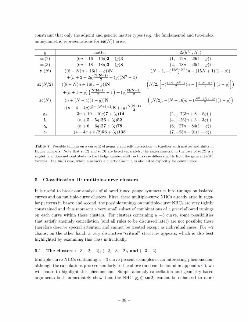
constraint that only the adjoint and generic matter types (e.g. the fundamental and two-indexantisymmetric representations for su(N)) arise.

g matter ∆(h1,1, Hu)

su(2) (6n+ 16− 16g)2 + (g)3 (1,−12n− 29(1− g))

su(3) (6n+ 18− 18g)3 + (g)8 (2,−18n− 46(1− g))

su(N) ((8−N)n+ 16(1− g))N (N − 1,−(15N−N2

2 )n− (15N + 1)(1− g))

+(n+ 2− 2g)N(N−1)2 + (g)(N2 − 1)

sp(N/2) ((8−N)n+ 16(1− g))N(N/2,

[−(15N−N2−2

2 )n−(

31N−N2

2

)(1− g)

])+(n+ 1− g)

(N(N−1)

2 − 1)

+ (g)N(N+1)2

so(N) (n+ (N − 4)(1− g))N(bN/2c,−(N + 16)n− (N

2−7N+1282 )(1− g)

)+(n+ 4− 4g)25−b(N+1)/2cS + (g)N(N−1)

2

g2 (3n+ 10− 10g)7 + (g)14 (2, [−7(3n+ 8− 8g)])

f4 (n+ 5− 5g)26 + (g)52 (4, [−26(n+ 3− 3g)])

e6 (n+ 6− 6g)27 + (g)78 (6,−27n− 84(1− g))

e7 (4− 4g + n/2)56 + (g)133 (7,−28n− 91(1− g))

Table 7. Possible tunings on a curve Σ of genus g and self-intersection n, together with matter and shifts inHodge numbers. Note that su(2) and su(3) are listed separately; the antisymmetric in the case of su(2) is asinglet, and does not contribute to the Hodge number shift, so this case differs slightly from the general su(N)

formula. The su(3) case, which also lacks a quartic Casimir, is also listed explicitly for convenience.

5 Classification II: multiple-curve clusters

It is useful to break our analysis of allowed tuned gauge symmetries into tunings on isolatedcurves and on multiple-curve clusters. First, these multiple-curve NHCs already arise in regu-lar patterns in bases; and second, the possible tunings on multiple-curve NHCs are very tightlyconstrained and thus represent a very small subset of combinations of a priori allowed tuningson each curve within these clusters. For clusters containing a −3 curve, some possibilitiesthat satisfy anomaly cancellation (and all rules to be discussed later) are not possible; thesetherefore deserve special attention and cannot be treated except as individual cases. For −2

chains, on the other hand, a very distinctive “critical” structure appears, which is also besthighlighted by examining this class individually.

5.1 The clusters (−3,−2,−2), (−2,−3,−2), and (−3,−2)

Multiple-curve NHCs containing a −3 curve present examples of an interesting phenomenon:although the calculations proceed similarly to the above (and can be found in appendix C), wewill pause to highlight this phenomenon. Simple anomaly cancellation and geometry-basedarguments both immediately show that the NHC g2 ⊕ su(2) cannot be enhanced to more

– 38 –

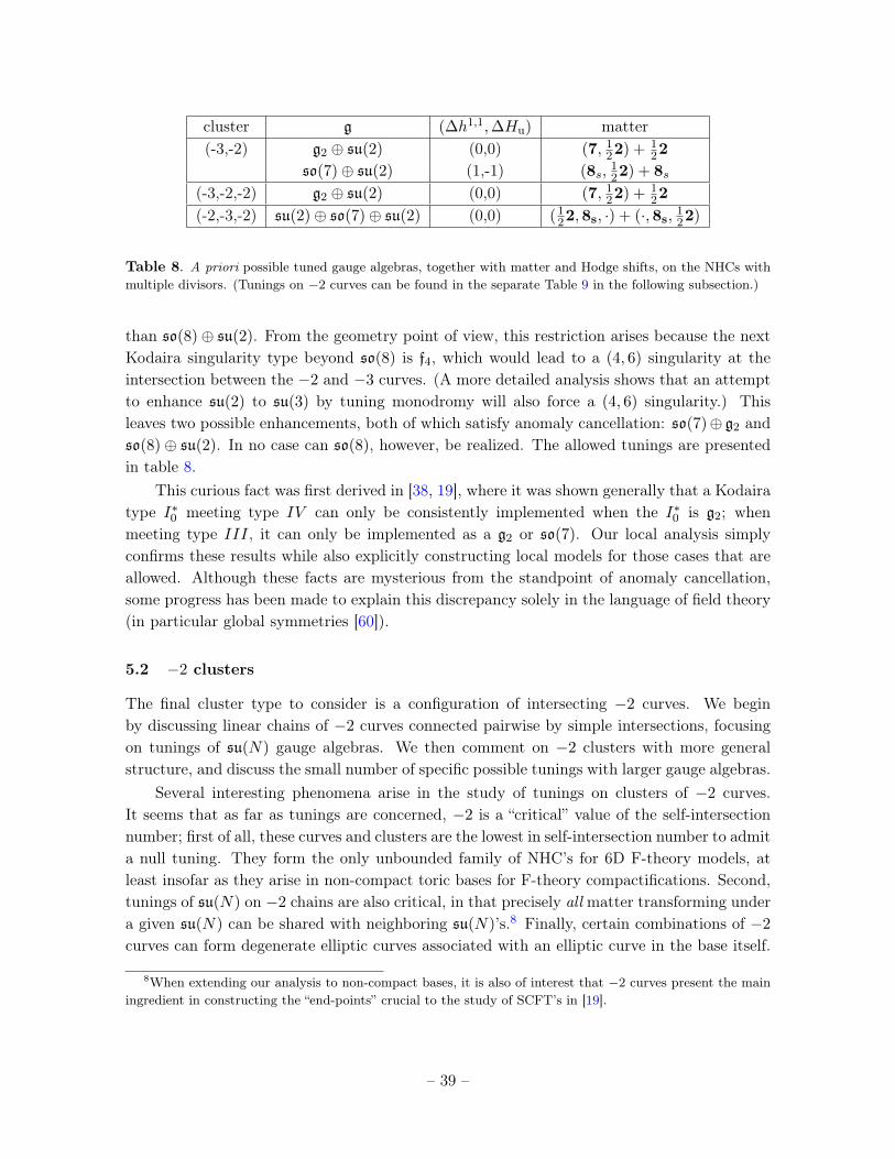
cluster g (∆h1,1,∆Hu) matter(-3,-2) g2 ⊕ su(2) (0,0) (7, 1

22) + 122

so(7)⊕ su(2) (1,-1) (8s,122) + 8s

(-3,-2,-2) g2 ⊕ su(2) (0,0) (7, 122) + 1

22

(-2,-3,-2) su(2)⊕ so(7)⊕ su(2) (0,0) (122,8s, ·) + (·,8s, 1

22)

Table 8. A priori possible tuned gauge algebras, together with matter and Hodge shifts, on the NHCs withmultiple divisors. (Tunings on −2 curves can be found in the separate Table 9 in the following subsection.)

than so(8)⊕ su(2). From the geometry point of view, this restriction arises because the nextKodaira singularity type beyond so(8) is f4, which would lead to a (4, 6) singularity at theintersection between the −2 and −3 curves. (A more detailed analysis shows that an attemptto enhance su(2) to su(3) by tuning monodromy will also force a (4, 6) singularity.) Thisleaves two possible enhancements, both of which satisfy anomaly cancellation: so(7)⊕ g2 andso(8)⊕ su(2). In no case can so(8), however, be realized. The allowed tunings are presentedin table 8.

This curious fact was first derived in [38, 19], where it was shown generally that a Kodairatype I∗0 meeting type IV can only be consistently implemented when the I∗0 is g2; whenmeeting type III, it can only be implemented as a g2 or so(7). Our local analysis simplyconfirms these results while also explicitly constructing local models for those cases that areallowed. Although these facts are mysterious from the standpoint of anomaly cancellation,some progress has been made to explain this discrepancy solely in the language of field theory(in particular global symmetries [60]).

5.2 −2 clusters

The final cluster type to consider is a configuration of intersecting −2 curves. We beginby discussing linear chains of −2 curves connected pairwise by simple intersections, focusingon tunings of su(N) gauge algebras. We then comment on −2 clusters with more generalstructure, and discuss the small number of specific possible tunings with larger gauge algebras.

Several interesting phenomena arise in the study of tunings on clusters of −2 curves.It seems that as far as tunings are concerned, −2 is a “critical” value of the self-intersectionnumber; first of all, these curves and clusters are the lowest in self-intersection number to admita null tuning. They form the only unbounded family of NHC’s for 6D F-theory models, atleast insofar as they arise in non-compact toric bases for F-theory compactifications. Second,tunings of su(N) on −2 chains are also critical, in that precisely all matter transforming undera given su(N) can be shared with neighboring su(N)’s.8 Finally, certain combinations of −2

curves can form degenerate elliptic curves associated with an elliptic curve in the base itself.

8When extending our analysis to non-compact bases, it is also of interest that −2 curves present the mainingredient in constructing the “end-points” crucial to the study of SCFT’s in [19].

– 39 –

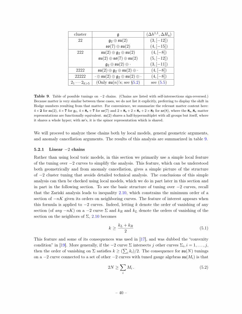
cluster g (∆h1,1,∆Hu)

22 g2 ⊕ su(2) (3, [−12])

so(7)⊕ su(2) (4, [−15])

222 su(2)⊕ g2 ⊕ su(2) (4, [−8])

su(2)⊕ so(7)⊕ su(2) (5, [−12])

g2 ⊕ su(2)⊕ · (3, [−11])

2222 su(2)⊕ g2 ⊕ su(2)⊕ · (4, [−8])

22222 · ⊕ su(2)⊕ g2 ⊕ su(2)⊕ · (4, [−8])

21 · · · 2k>5 (Only su(n)’s; see §5.2) see (5.5)

Table 9. Table of possible tunings on −2 chains. (Chains are listed with self-intersections sign-reversed.)Because matter is very similar between these cases, we do not list it explicitly, preferring to display the shift inHodge numbers resulting from that matter. For convenience, we summarize the relevant matter content here:4×2 for su(2), 4×7 for g2, 4×8s +7 for so(7) and 2×8s + 2×8c + 2×8f for so(8), where the 8s,8c matterrepresentations are functionally equivalent. su(2) shares a half-hypermultiplet with all groups but itself, whereit shares a whole hyper; with so’s, it is the spinor representation which is shared.

We will proceed to analyze these chains both by local models, general geometric arguments,and anomaly cancellation arguments. The results of this analysis are summarized in table 9.

5.2.1 Linear −2 chains

Rather than using local toric models, in this section we primarily use a simple local featureof the tuning over −2 curves to simplify the analysis. This feature, which can be understoodboth geometrically and from anomaly cancellation, gives a simple picture of the structureof −2 cluster tuning that avoids detailed technical analysis. The conclusions of this simpleanalysis can then be checked using local models, which we do in part later in this section andin part in the following section. To see the basic structure of tuning over −2 curves, recallthat the Zariski analysis leads to inequality 2.10, which constrains the minimum order of asection of −nK given its orders on neighboring curves. The feature of interest appears whenthis formula is applied to −2 curves. Indeed, letting k denote the order of vanishing of anysection (of any −nK) on a −2 curve Σ and kR and kL denote the orders of vanishing of thesection on the neighbors of Σ, 2.10 becomes

k ≥ kL + kR2

(5.1)

This feature and some of its consequences was used in [17], and was dubbed the “convexitycondition” in [19]. More generally, if the −2 curve Σ intersects j other curves Σi, i = 1, . . . , j,then the order of vanishing on Σ satisfies k ≥ (

∑i ki)/2. The consequence for su(N) tunings

on a −2 curve connected to a set of other −2 curves with tuned gauge algebras su(Mi) is that

2N ≥∑i

Mi . (5.2)

– 40 –

This condition follows immediately from anomaly cancellation, since at every intersectionthere is a hypermultiplet of shared matter in the (N,Mi) representation, and Σ only carries2N matter fields in the fundamental representation. Thus, this simple convexity conditionnaturally captures the constraints of anomaly cancellation.

Comparison to harmonic functions yields some immediate insight. For instance, on aclosed or infinite chain of −2 curves, a (0, 0, n) tuning on any divisor forces a (0, 0, n) tuningon every divisor. More generally, imagine that a curve Σ supports a tuned su(n) gauge algebra,associated with vanishing orders of (f, g,∆) of (0, 0, n). Now consider a linear chain of k (−2)-curves connected in sequence to Σ, with curves labeled by Σ1, · · · ,Σk, with Σk = Σ. Theorder of vanishing of ∆ on Dl then satisfies nl ≥ dn l

ke. We can recover from this rule theinfinite case. Note that in some cases the inequality cannot be saturated .

The local rule (5.2) gives a clear bound on possible tunings of −2 curves combined in anarbitrary cluster. In the following section we prove using Tate tunings that, at least at the locallevel of pairwise intersections, every tuning of a combination of su(N) algebras on intersectingdivisors that is allowed from (5.2) can be realized through a Weierstrass construction, so atleast locally there is a perfect match between the constraints of the low-energy field theoryand F-theory. Here we proceed simply using (5.2) to make some observations about possibletunings of su(N) combinations on −2 clusters.

The local rule (5.2) has simple consequences for tunings over any linear chain of −2 curves.In particular, on a linear chain of −2 curves Σi, the sequence of gauge algebras su(Ni) mustbe convex, with each Ni greater or equal to the average of the adjoining Ni−1, Ni+1. Thisconstraint gives a systematic framework for analyzing local tunings on any linear chain of −2

curves. Note, however, that the set of possible tunings even on a single isolated −2 is a prioriinfinite, when no further constraints from neighboring divisors are taking into account. Thefinite bound on possible tunings of curves of self-intersection −2 or above is discussed in thefollowing section and §9, in the context of intersection with other curves in the base. For 6Dsupergravity models with a compact base, the actual number of possible tunings is alwaysfinite, while for 6D SCFT’s the family of possible tunings is infinite. Similarly, for 6D SCFT’sthere is no bound on the number of possible −2 curves that can be combined in a chain, whilefor compact supergravity models there is a finite bound.

Given this structure, we can simply classify all su(N) tunings over clusters of −2 curves.The tunings allowed are precisely those that satisfy (5.2). If we have a set of l curves Σi

that carry gauge algebras su(Ni), with intersection numbers Iij ∈ {0, 1}, then the total gaugealgebra is

⊕i su(Ni) , (5.3)

the matter content is ∑i,j:Iij=1

(Ni,Nj) , (5.4)

– 41 –

and the shift in Hodge numbers is

∆(h1,1, h2,1) =

∑i

(Ni − 1),∑i

(−N2i − 1) +

∑i,j:Iij=1

(NiNj)

. (5.5)

The “critical” nature of −2 chains is particularly apparent when the inequality (5.2)is saturated. In this case, all of the 2N fundamental matter fields on Σ are involved inbifundamental matter fields. An interesting feature of this is that there is an almost perfectcancellation between the number of vector and hyper multiplets. In particular, for a closedchain of −2 curves, with su(N) tuned on each, we have a contribution to Hcharged − V ofprecisely 1 for each −2 curve. This interesting possibility is discussed further in a related setof circumstances in the following subsection.

5.2.2 Nonlinear −2 clusters

We can use (5.2) to describe su(N) tunings on more complicated configurations of −2 curves,which may include branching or loops. Remarkably, this simple averaging rule strongly con-strains the kinds of clusters that can support tunings, revealing a potentially very interestingstructure.

First, consider a −2 curve Σ that is connected to c linear chains of −2 curves of lengthli − 1. Assume that su(N) is tuned on Σ. Then from the above analysis, each of the curvesconnected to Σ from the linear chains must support at least a gauge factor su(dN(li− 1)/lie).From (5.2), however, the sum of the resultingMi has an upper bound of 2N . This immediatelybounds the types of chains that can be connected to Σ. A chain of length 1 contributes atleast N/2 to

∑iMi, a chain of length 2 contributes at least 2N/3, etc.. Thus, we can have at

most four chains connected to Σ, and this is possible only for chains of length one. If we have3 chains, it is straightforward to check that the allowed lengths are (1, 1, l − 1) for arbitraryl, (1, 2, l − 1) for l ≤ 6, (1, 3, 3), and (2, 2, 2). Thinking of these configurations as Dynkindiagrams, the extremal cases in this enumeration correspond precisely with the classificationof degenerate elliptic curves associated with affine Dynkin diagrams D4, Dl+1, and En [29].Examples of these degenerate elliptic curves are illustrated in Figure 2. All of these nontrivial−2 curve configurations can be realized, for example on rational elliptic surfaces [61, 62].Specific examples of such realizations were encountered in the classification of C∗ bases in[15].

In the extremal cases, we have a situation where combinations of su(N) can be tuned onthese divisors with a contribution to Hcharged − V that is independent of N . For example,on the (2, 2, 2) configuration corresponding to E6, we can tune a gauge algebra su(3N) on Σ,su(2N) on the components of the chains that intersect Σ, and su(N) on the terminal links inthe chains. This presents an apparent puzzle, since in a compact base only a finite number oftunings are possible and we would expect higher-rank tuning to require more moduli.

Weierstrass models for the extremal −2 clusters can be analyzed using the methodologyused in [15]. For example, for the case of a −2 curve Σ intersecting four other −2 curves, in

– 42 –

local coordinates where the other curves intersect Σ at w = 0, 1, 2,∞, the generic Weierstrassmodel takes the form

f = f0 + f2ζz2 + f4ζ

2z4 + · · · (5.6)

g = g0 + g2ζz2 + g4ζ

2z4 + · · · , (5.7)

where ζ = w(w − 1)(w − 2). We can set ∆ = O(z2) by tuning g0 to cancel in the leadingterm. This gives a gauge algebra of su(2) on Σ and no gauge algebra on the other curves.The shift in H0 is then given by ∆H0 = V −Hcharged = −5. This appears surprising as wehave only tuned one modulus, but keeping careful track of extra moduli from −2 curves thisis correct; once we have done this tuning, the discriminant identically vanishes on the fouradditional curves, so they are no longer counted as contributing to N−2 as discussed in §2.5.We can further tune g2 so that the next term in the discriminant vanishes. This then givesan su(4) on Σ and an su(2) on the other four curves. We now have V −Hcharged = −5 again,but we have nonetheless tuned a modulus. Repeating this, we use one modulus each time weincrease the algebra on Σ by N → N + 1. This represents an apparent disagreement betweenthe moduli needed for Weierstrass tuning and anomaly cancellation.

Some insight can be gleaned into what is transpiring in these situations by observingthat these −2 configurations are essentially degenerate genus one curves that satisfy Σ · Σ =

−K · Σ = 0. On a smooth curve of this type, the only matter would be a single adjointrepresentation of su(N), giving Hcharged − V = 1, independent of N . When the smoothgenus one curve degenerates into a combination of −2 curves, the resulting configuration ofsu(N) groups is precisely that realized on the extremal −2 clusters, with no matter in thefundamental, and bifundamental matter at the intersection points. Indeed, the multiplicityof N that is tuned on each −2 curve for each extremal cluster associated with a degenerateelliptic curve is precisely the proper multiplicity to give the elliptic curve. Thus, this canbe thought of in each of these cases as tuning an su(N) on the elliptic curve and taking adegenerate limit.

The tuning of a single degree of freedom for each increase in N can be understood as themotion of a single seven-brane in the transverse direction to the genus one curve Σ. The factthat N can only be tuned to a certain maximum value for the smooth genus one curve Σ withΣ · Σ = 0 follows from the fact that ∆ = −12K; there is always some maximum N such that−12K − NΣ is effective. In a compact base with an extremal −2 cluster, this correspondsto the fact that the Weierstrass expansion terminates and only a finite number of tunings arepossible. For example, tuning two of these clusters, with the sets of four additional −2 curvesin each cluster connected pairwise by −1 curves gives a base studied in [15], which has theunusual future of supporting a generic U(1) factor associated with a higher rank Mordell-Weilgroup. This structure may be a clue to the anomalous anomaly behavior. In this compactbase, f, g in (5.6) only go out to order z8, z12 respectively, giving a bound on the gauge groupthat can be tuned.

A closed loop of −2 curves fits into this framework as the affine Al−1 Dynkin dia-gram/degenerate elliptic curve. We comment on this further in §6.5. Note also that in

– 43 –

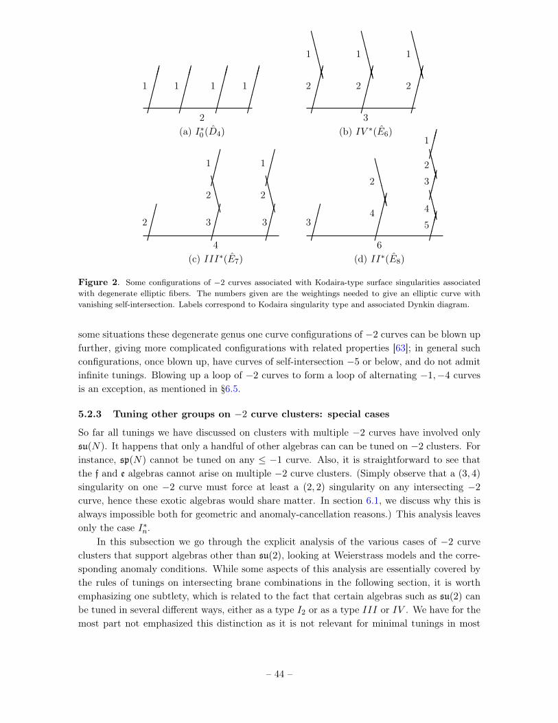
(a) I∗0 (D4)

2������

1

������

1

������

1

������

1

(b) IV ∗(E6)

3������

CCCCCC

2

1

������

CCCCCC

2

1

������

CCCCCC

2

1

(c) III∗(E7)

4����

2����

����

CCCC

3

2

1

����

����

CCCC

3

2

1

(d) II∗(E8)

6����

3������

CCCCCC

4

2

����5

CCCC

4����3

CCCC

2����1

Figure 2. Some configurations of −2 curves associated with Kodaira-type surface singularities associatedwith degenerate elliptic fibers. The numbers given are the weightings needed to give an elliptic curve withvanishing self-intersection. Labels correspond to Kodaira singularity type and associated Dynkin diagram.

some situations these degenerate genus one curve configurations of −2 curves can be blown upfurther, giving more complicated configurations with related properties [63]; in general suchconfigurations, once blown up, have curves of self-intersection −5 or below, and do not admitinfinite tunings. Blowing up a loop of −2 curves to form a loop of alternating −1,−4 curvesis an exception, as mentioned in §6.5.

5.2.3 Tuning other groups on −2 curve clusters: special cases

So far all tunings we have discussed on clusters with multiple −2 curves have involved onlysu(N). It happens that only a handful of other algebras can can be tuned on −2 clusters. Forinstance, sp(N) cannot be tuned on any ≤ −1 curve. Also, it is straightforward to see thatthe f and e algebras cannot arise on multiple −2 curve clusters. (Simply observe that a (3, 4)

singularity on one −2 curve must force at least a (2, 2) singularity on any intersecting −2

curve, hence these exotic algebras would share matter. In section 6.1, we discuss why this isalways impossible both for geometric and anomaly-cancellation reasons.) This analysis leavesonly the case I∗n.

In this subsection we go through the explicit analysis of the various cases of −2 curveclusters that support algebras other than su(2), looking at Weierstrass models and the corre-sponding anomaly conditions. While some aspects of this analysis are essentially covered bythe rules of tunings on intersecting brane combinations in the following section, it is worthemphasizing one subtlety, which is related to the fact that certain algebras such as su(2) canbe tuned in several different ways, either as a type I2 or as a type III or IV . We have for themost part not emphasized this distinction as it is not relevant for minimal tunings in most

– 44 –

cases, and is not easy to understand in terms of the low-energy theory, however it is relevantin these cases, which serve as an illustration of how these distinctions are relevant in specialcases.

In more detail, the Kodaira cases to consider are combinations of I∗0 tunings with su(2)

tuned as either type III or IV . Let us see why this is. To understand why I∗≥1 cannot betuned, suffice it to say that geometrically, it forces a (4, 6) singularity at the intersection pointwith any other −2 curve. Although this could be demonstrated directly, we note here that itwill follow from our geometric arguments that even so(8) cannot be tuned on any −2 cluster;the monomials in f and g that must be set to zero to achieve an so(8) are a strict subset ofthose which must be set to zero in tuning so(9). From the anomaly cancellation standpoint,this statement is perfectly consistent, because we expect all matter to be 8 half-hypermultipetsof an su(2) forced on an adjacent curve, and therefore the dimension of the matter sharedwith su(2) cannot exceed 8, but of course would be for so(≥ 9). In fact, it is impossible foran I∗0 to appear next to anything but su(2). This is because an I∗0 (2, 3) singularity forces atleast a (1, 2) singularity on any intersecting −2 curve. Attempting to tune su(3) with a IVsingularity requires that g2 be a perfect square. However, a toric analysis for two intersecting−2 curves reveals that g2 has a lowest order term of order w3, which cannot be the lowest orderterm of a perfect square. Eliminating this monomial directly produces a (4, 6) singularity atthe intersection point. This conclusion is also reasonable from the field theory point of view:the fundamental of su(3) is not self-conjugate, and therefore the matter shared with it can beat most 6-dimensional.

In summary, the only tunings on −2 curve clusters that contain algebras other than su(N)

are combinations of I∗0 and III/IV su(2)’s. In fact, the averaging rule implies that tuningscontaining one I∗0 component may only occur in chains with ≤ 5 curves. (On larger clusters,the averaging rule implies that the (2, 3, 6) singularity would persist to at least the nearestneighbor, immediately yielding a (4, 6) singularity at the intersection point.) Therefore, ourtask is to classify the allowed combinations of su(2), g2, so(7), and so(8). We will find thatonly g2 and so(7) can be realized, but not so(8).9 As discussed above, an I∗0 tuning necessarilyforces at least a III singularity on an intersecting −2 curve, so we will not encounter anyisolated I∗0 tunings. (This geometrical constraint is not yet well characterized in terms of thelow-energy field theory; see §6.3)

Let us now classify these tunings: namely, a single g2, so(7), or so(8) together with itsneighbors, which must be su(2)’s. This must occur on a chain of length ≤ 5. We will constructthese models in order of increasing length of chain, starting on a configuration (Σ1,Σ2) of twointersecting −2 curves, and progressing to a chain (Σ1, · · · ,Σ5) of five −2 curves in a linearconfiguration. For each of these four configurations, we tune a g2, then attempt to enhanceto so(7) or so(8). Because we will immediately find that so(8) cannot be tuned, we will notconsider it on any configuration but the first. (Configurations with additional −2 curves have

9This matches with the low-energy constraint from global symmetries [60], as discussed in more detail in§6.3.

– 45 –

strictly fewer monomials, so any obstruction to tuning on smaller configurations will applytrivially to larger configurations as well.) To set notation, we will use {z = 0} to be a localdefining equation for the curve Σ on which the type I∗0 singularity is tuned; any intersectingcurve of interest we will take to be defined as {w = 0}. We will consider f =

∑i,j fi,jz

iwj

and similarly for g; when discussing orders of vanishing on e.g. Σ = {z = 0}, we will useterms fi,· and gi,· with one blank subscript to refer to functions of w in an implicit expansionf =

∑i fi,·(w)zi. Similarly f·,j refers to an implicit expansion f =

∑i f·,j(z)w

j . While weonly discuss linear chains here explicitly, a similar analysis governs the tuning of an I∗0 factoron a small branched −2 cluster; details are left to the reader.

Case 1 (a): g2 on (−2,−2). To implement the tuning g2 on Σ1, we must impose(ordΣ1f, ordΣ1g) = (2, 3), so for f we eliminate 1 + 2 degrees of freedom in setting f0,· andf1,· to zero, while for g we eliminate 1 + 2 + 4 degrees of freedom in setting g0,·, g1,·, and g2,·to zero. Now let us examine f2,· =

∑4i=1 f2,iw

i and g3,· =∑6

i=2 g3,izi. By inspection, the

geometry does not force a non-generic factorization, so we have indeed tuned g2, and not oneof the other I∗0 cases. The removal of these monomials forces (ordΣ2f, ordΣ2g) = (1, 2), sothat we obtain an su(2) neighbor. As a check, note that implementing this tuning fixes 10

monomials as well as two −2 curve moduli, which yields a shift in Hu of −12, consistent withanomaly cancellation. No further complications have arisen in this instance.

(b): so(7) Enhancing this tuning to so(7), we impose

f2 = B −A2 (5.8)

g3 = −AB (5.9)

which is most generically achieved by setting A = A1w+A2w2 and B = B1w+B2w

2 +B3w3 +

B4w4, for a total loss of 9−6 = 3 degrees of freedom. Note that all coefficients f2,i and g3,i will

generally remain nonzero. This implies that the orders of (f, g) on Σ2 remain (1, 2), so thatthe neighboring su(2) remains type III. It is worth mentioning that these calculations agreewith the anomaly calculations of shifts in Hu when one tunes the g2⊕ su(2) −→ so(7)⊕ su(2)

combination, provided that it is one of the four 8s representations of so(7) that is also chargedas a fundamental under su(2)–not the 7f . This bifundamental matter is consistent with theprocess of Higgsing back to g2 as it leaves the 7 unharmed to play the role of the 7 fundamentalof g2. Moreover, this matches with the global symmetry analysis of [60], which indicates thatthe 8s representation must be shared instead of the 7 representation.

(c): so(8): Forbidden This tuning is impossible, as mentioned above; hence all so(8)

tunings will be impossible on larger −2 chains. To see this in this context, recall that toenhance the tuning to so(8), we require the more stringent factorization condition

f2 = AB − (A+B)2 (5.10)

g3 = AB(A+B) (5.11)

which is most generically achieved by setting A = A1w + A2w2, B = B1w + B2w

2. Noticethat this removes all monomials zawb in g with b ≤ 3, hence a+ b ≥ 6. Therefore the order of

– 46 –

g at the intersection point between the −2 curves is at least 6. Notice as well that this tuningremoves the order z2 term in f . Combining these facts, this tuning attempt would yield a(4, 6) singularity where the −2 curves meet.

Case 2 (a,i): g2 on Σ1 of (−2,−2,−2). In this cluster we may tune either on thefirst curve Σ1 or the middle curve Σ2. The former presents distinct differences, which wewill discuss first, after which we will move on to discuss the tuning on Σ2, which proceedsanalogously to the tuning on (−2,−2).

Let us now implement the tuning on Σ1. The additional complication will be the possibil-ity of a forced gauge algebra on the final curve Σ3. On Σ2, the effect is a type IV singularitywith g2 consisting of a single monomial. In fact, this monomial is z3 in a defining coordinatez for Σ2, so we will never encounter the issue of an su(3) on Σ2. On Σ3, there is only an IItype singularity, which does not produce a gauge algebra. This tuning has proceeded withoutobstruction.

(a,ii): so(7): Forbidden Since f2,· = f2,1w+ f2,2w2 and g3,· = g3,2w

2 + g3,3w3 + g3,4w

4,the required factorization condition is satisfied by the choice A = A1w, B = B1w + B2w

2.Note that this requires the w4 term in g3,· to vanish, in addition to imposing a relation amongthe remaining coefficients. We lose 2 degrees of freedom, as expected from the point of viewof anomaly calculations above. This factorization constraint removes the single monomial ofin g that is order 2 over Σ3 , leading to a III singularity on Σ3. An su(2) on Σ3 would haveto share more matter than it carries in the first place; therefore this enhancement, as well assubsequent ones, are inconsistent. In more geometric terms, a (4, 6) singularity appears atΣ1 · Σ2.

(b,i) g2 on Σ2 Attempting to tune I∗0 on the middle curve Σ2 proceeds without difficulty,in complete analogy to tuning on the Σ1 in the configuration (−2,−2) of case 1. Implementinga tuning of g2 on the middle curve Σ2, we investigate the forced tunings on its neighbors Σ1

and Σ3. (By symmetry, it suffices to consider only Σ1, which incurs an (f, g) = (1, 2) typeIII singularity.) One can confirm that there is generic factorization on Σ2, so we are indeedin the g2 case.

(b,ii): so(7) Since (on Σ2) f2,· = f2,1w+f2,2w2+f2,3w

3 and g3,· = g3,2w2+g3,3w

3+g3,4w4,

the relevant factorization condition can be achieved with A = A1w, B = B1w+B2w2 +B3w

3,for a loss of 2 degrees of freedom. This is consistent with anomaly calculations, and moreoverthe singularities on the adjacent curves remain type III.

Case 3 (a,i): g2 on Σ1 of (−2,−2,−2,−2) The novel contribution to this cluster is thepossibility of tuning on the initial curve Σ1. However, this is impossible. The pathology ofthis attempted tuning is visible even without investigating monomials. A (2, 3, 6) singularityon Σ1 will, by the averaging rule, immediately produce at least a (2, 3, 6) singularity on Σ2,leading to an unacceptable (4, 6) singularity at Σ1 ·Σ2. Indeed, this same logic shows that notuning of I∗0 is possible on a chain of ≥ 6 −2 curves, as there is no curve in this chain thatwith have fewer than 3 additional −2 curves to one side. We reemphasize: even g2 cannot betuned here.

(b,i): g2 on Σ2 of (−2,−2,−2,−2). In this case, we will tune on Σ2, which is quite anal-

– 47 –

ogous to tuning on Σ1 of the configuration (−2,−2,−2). We find no additional restrictions,but we the presence of the −2 curve Σ1 leads to the presence of another (type III) su(2)

neighbor. Examining first the effect on Σ1, a g2 produces the expected III or (f, g) = (1, 2)

singularity. On Σ3, the effect is a type IV singularity with g·,2 consisting of a single monomial,and on Σ4, there is only a type II type singularity, as in case (a, i) above.

(b,ii): so(7): Forbidden This is already assured from the analysis of case 2, as we havemerely added another −2 curve, which can only add constraints.

Case 4 (a): g2 on (−2,−2,−2,−2,−2). The previous analysis already shows that wecannot tune an I∗0 singularity anywhere but the middle curve; otherwise, there would be astring of ≥ 3 −2 curves to one side of the I∗0 , which would force a (4, 6) singularity. Thus, ourgoal is simply to verify that a g2 can be tuned on the middle curve Σ3, in precise analogy totuning on Σ2 of case 3. We already know that tuning so(7) and so(8) tunings are forbiddenin this context, because this case is obtained from the previous one by an additional blowupat the endpoint −1 curve of the local model. The task, then, is simply to verify that thegeneric I∗0 g2 singularity can be consistently imposed. By investigating the monomials, onecan implement this tuning, finding that on Σ3, f2,· = f2,2w

2 and g3,· = g3,2w2 +g3,3w

3 +g3,4w4

(in a defining coordinate w for Σ2), which implies that no factorization is generically forced,so this tuning belongs in the g2 subcase of I∗0 tunings, as desired. Moreover, on Σ2, thereis a forced IV singularity, for which g·,2 = g3,2z

3, yielding su(2). Similarly for Σ4. Thisensures an su(2) is adjacent to the tuned g2 on either side. As to Σ1,5, each carries a type IIsingularity–in other words, no tuned algebra. This ensures that such a g2 tuning can in factbe realized, completing the desired classification.

6 Classification III: connecting curves and clusters

At this point, we have investigated tunings over individual curves or non-Higgsable clusters.To go further, we would like to determine constraints on what groups can be tuned over inter-secting divisors. In particular, low-energy anomaly cancellation conditions and correspondingF-theory geometric conditions impose clear constraints on what groups can be tuned over in-tersecting divisors. At this point we are unaware of any specific constraints on global modelsthat go beyond conditions that can be expressed in terms of gauge groups tuned on a singledivisor Σ and its immediate neighbors (i.e., divisors intersecting Σ). Thus, it may be thatdetermining local constraints on such configurations may be sufficient to determine the fullset of global tunings that is possible. We do not attempt to prove the completeness of localconditions here, but focus in this section on various conditions that constrain tunings that arepossible on multiple intersecting curves.

In §6.1 we give a simple set of arguments that show that there are only 5 (families of) pairsof gauge groups that can be tuned on a pair of intersecting divisors. In §6.2, we determineconstraints on these families in terms of the self-intersections of the curves involved and thegroup types. In §6.3 we consider a more general set of constraints on a curve Σ that intersects

– 48 –

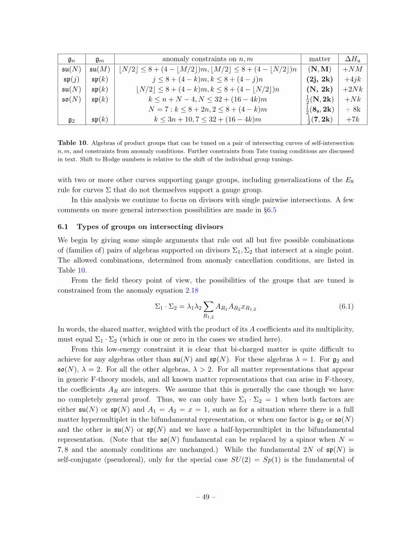
gn gm anomaly constraints on n,m matter ∆Hu

su(N) su(M) bN/2c ≤ 8 + (4− bM/2c)m, bM/2c ≤ 8 + (4− bN/2c)n (N,M) +NM

sp(j) sp(k) j ≤ 8 + (4− k)m, k ≤ 8 + (4− j)n (2j, 2k) +4jk

su(N) sp(k) bN/2c ≤ 8 + (4− k)m, k ≤ 8 + (4− bN/2c)n (N, 2k) +2Nk

so(N) sp(k) k ≤ n+N − 4, N ≤ 32 + (16− 4k)m 12(N,2k) +Nk

N = 7 : k ≤ 8 + 2n, 2 ≤ 8 + (4− k)m 12(8s,2k) + 8k

g2 sp(k) k ≤ 3n+ 10, 7 ≤ 32 + (16− 4k)m 12(7,2k) +7k

Table 10. Algebras of product groups that can be tuned on a pair of intersecting curves of self-intersectionn,m, and constraints from anomaly conditions. Further constraints from Tate tuning conditions are discussedin text. Shift to Hodge numbers is relative to the shift of the individual group tunings.

with two or more other curves supporting gauge groups, including generalizations of the E8

rule for curves Σ that do not themselves support a gauge group.In this analysis we continue to focus on divisors with single pairwise intersections. A few

comments on more general intersection possibilities are made in §6.5

6.1 Types of groups on intersecting divisors

We begin by giving some simple arguments that rule out all but five possible combinationsof (families of) pairs of algebras supported on divisors Σ1,Σ2 that intersect at a single point.The allowed combinations, determined from anomaly cancellation conditions, are listed inTable 10.

From the field theory point of view, the possibilities of the groups that are tuned isconstrained from the anomaly equation 2.18

Σ1 · Σ2 = λ1λ2

∑R1,2

AR1AR2xR1,2 (6.1)

In words, the shared matter, weighted with the product of its A coefficients and its multiplicity,must equal Σ1 · Σ2 (which is one or zero in the cases we studied here).

From this low-energy constraint it is clear that bi-charged matter is quite difficult toachieve for any algebras other than su(N) and sp(N). For these algebras λ = 1. For g2 andso(N), λ = 2. For all the other algebras, λ > 2. For all matter representations that appearin generic F-theory models, and all known matter representations that can arise in F-theory,the coefficients AR are integers. We assume that this is generally the case though we haveno completely general proof. Thus, we can only have Σ1 · Σ2 = 1 when both factors areeither su(N) or sp(N) and A1 = A2 = x = 1, such as for a situation where there is a fullmatter hypermultiplet in the bifundamental representation, or when one factor is g2 or so(N)

and the other is su(N) or sp(N) and we have a half-hypermultiplet in the bifundamentalrepresentation. (Note that the so(N) fundamental can be replaced by a spinor when N =

7, 8 and the anomaly conditions are unchanged.) While the fundamental 2N of sp(N) isself-conjugate (pseudoreal), only for the special case SU(2) = Sp(1) is the fundamental of

– 49 –

su(n) self-conjugate. Thus, field theory considerations seem immediately to restrict to the 5possibilities in Table 10.

We can show directly in F-theory using a local monomial analysis that indeed the fivepossibilities in Table 10 are the only combinations of algebras on intersecting divisors thatadmit a tuning in the Weierstrass model. We begin by showing that f4 cannot live on a curvethat intersects another curve supporting any nontrivial algebra. To begin, let us label thecurves of f4 and its neighbor g as Σ1 and Σ2 respectively. Now notice that f4 corresponds toa (3, 4) singularity. If a non-trivial algebra other than one in the In series appeared on Σ2,it would have to be at least a (1, 2) singularity–immediately leading to a (4, 6) singularity atΣ1 · Σ2. Thus, such tunings are inconsistent. It remains only to prove that a I≥2 algebracannot appear on Σ2, for which it will be sufficient to rule out just I2, i.e. an su(2) tunedby (0, 0, 2). By thinking in toric monomials, it is easy to see why this is inconsistent with a(3, 4, 8) tuning on Σ1. Let w be a local coordinate on Σ1 such that Σ2 = {w = 0}, and viceversa for z and Σ1 = {z = 0}. Then we can expand f , g, and ∆ in Taylor series in z and w.By hypothesis, f contains no monomials with powers of z lower than z3, and g contains nonewith powers lower than z4. To tune ∆ to order 2 on Σ2, we must require the vanishing of both∆0 and ∆1 in the expansion ∆ =

∑i=0 ∆iw

i. For ∆0 ∼ f30 + g2

0, this implies f0 ∝ φ2 andg0 ∝ φ3 for some expression φ. Immediately we see that f0 must be a perfect square, whichforces us to exclude the monomial w0z3; moreover, for g0 to be a perfect cube, the coefficientsin g of both w0z4 and w0z5 must be zero.

Now let us impose the constraint ∆1 ∼ f20 f1 + g0g1 = 0. The lowest order (in z) term in

f20 f1 is now z11 (4 + 4 + 3) whereas the lowest order term in g0g1 is z10 (6 + 4). The requiredcancellation between these terms can only occur, then, if g1 vanishes to order at least 5 insteadof 4. But now this putative tuning is in serious trouble. We have removed from f the singlemonomial w0z3 with m+ n < 4 (where wmzn). Moreover, we have removed from g the threemonomials with m + n < 6. This guarantees a (4, 6) singularity at Σ1 · Σ2, as we expectedto find. This proves that no gauge algebra can be tuned on a divisor intersecting a divisorcarrying a singularity of order (3, 4) or higher.

A similar analysis shows that divisors intersecting other divisors carrying the groups withalgebras so(n), g2 can only have sp(n) algebras. If we assume Σ1 carries a gauge algebrawith (f, g) vanishing to orders (2, 3), we similarly analyze f0, g0 at leading orders in z, etc.. Asecond curve Σ2 intersecting Σ1 cannot carry a (2, 3) singularity or we immediately have a (4, 6)

singularity at the intersection point. We thus need only consider gauge algebras su(n), sp(n)

on Σ2. We consider In type singularities. As above, we have f0 ∝ φ2, g0 ∝ φ3. For an su(n)

algebra the split condition dictates that we must have φ a perfect square φ = φ20. But then z|φ0,

z4|f0 and similarly z6|g0. To tune an su(3) we have [33] f1 ∼ φ0ψ1, g1 ∼ φf1, g2 ∼ ψ21 + φf2,

and since g2 and φf2 scale at least as z3, z4, z2|ψ1, which means z3|f1, z5|g1, z

4|g2, so we geta (4, 6) singularity at the intersection. A similar effort to tune an su(3) through a type IVsingularity would give a term z3 in g2, which implies that g2 is not a perfect square so themonodromy gives an su(2) algebra on any curve with a type IV singularity intersecting asingularity of order (2, 3).

– 50 –

This completes the demonstration that the only possible pairs of nontrivial algebras thatcan be realized on intersecting curves are those in Table 10. Note that the analysis herewas independent of the dimension of the base, so the same result holds for 4D F-theorycompactifications.

6.2 Constraining groups on intersecting divisors

We now consider the possible combinations of gauge groups that can actually be realizedfor the five possible pairings from Table 10. In each case we compare the constraints fromanomaly cancellation to a local Tate analysis, as was done for single curves in §4.3. We takethe self-intersections of the two curves to be Σ1 · Σ1 = n, Σ2 · Σ2 = m, and we are assumingthat Σ1 · Σ2 = 1. We consider the various cases in turn, indicating potential swamplandcontributions in each case.

sp(j)⊕ sp(k) (no swamp):We begin with the case Sp(j = N/2) × Sp(k = M/2), where the analysis is simplest.

In this case, we expect a single (full) bifundamental hypermultiplet in the (N,M) = (2j,2k)

representation. The number of fundamentals on each of the two curves is, from Table 4,16 + (8− 2j)n, 16 + (8− 2k)m respectively. We therefore have the constraints from anomalycancellation

j ≤ 8 + (4− k)m,

k ≤ 8 + (4− j)n . (6.2)

Here, the self-intersections satisfy n,m ≥ −1, since sp(k) cannot be tuned on a −2 curve.Now let us consider the Tate model. Tuning sp(j) on a curve of self-intersection n requires

tuning the a coefficients (a1, a2, a3, a4, a6) to vanish to orders (0, 0, j, j, 2j). The weakestconstraint comes from the a4 condition. From (4.35), we see that the degrees of the coefficientsin a4 are deg(a4(s)) = 8 + n(4− s). Imposing both constraints, we see that a4 can be writtenin terms of monomials zswt subject to the conditions that t ≤ 8 + (4− s)n, s ≤ 8 + (4− t)m.Tuning the algebras sp(j) ⊕ sp(k) on our curves of self-intersections n,m requires having amonomial in a4 with degrees s = j, t = k, and we see that such a monomial exists if andonly if the constraints (6.2) are satisfied. This shows that in a local model, using the Tateconstruction, all possible sp(j) ⊕ sp(k) algebras consistent with anomaly constraints can betuned on a pair of intersecting curves.

su(2j)⊕ su(2k) (no swamp):A similar analysis can be carried out in the other cases of Table 10. We next consider

SU(N) × SU(M). If N,M are both even, with N = 2j,M = 2k, the tuning is precisely likethat of the Sp(j)×Sp(k) case just considered, except for the tuning of a2 to first order. The a2

tuning is always possible, so it cannot affect the conclusion, and so for even N,M everythingthat is allowed from anomalies can be realized using Tate. Note that for these algebras, wecan have in particular n = m = −2.

su(2j + 1)⊕ su(2k) (apparent swamp):

– 51 –

Next consider the case N = 2j + 1,M = 2k. In this case, the constraint from a4 is justas (6.2) but with j replaced by j + 1. But there must also either be at least one monomial ina3 of order at least j in z or a monomial in a6 of order at least 2j + 1, or else the symmetryautomatically enhances to SU(N + 1). The conditions that must be satisfied are then (a4 and(a3 or a6)), where

a4 : j ≤ 7 + (4− k)m, k ≤ 8 + (3− j)na3 : j ≤ 6 + (3− k)m, k ≤ 6 + (3− j)n (6.3)

a6 : 2j + 1 ≤ 12 + (6− 2k)m, 2k ≤ 12 + (5− 2j)n .

Some of these conditions imply others. In particular, the a6 condition on j is always strongerthan the a4 condition on j, and the a3 condition on k always implies the a4 condition on k.Nonetheless, the analysis is a bit subtle as different combinations are ruled in or out in differentways. For example, su(3)⊕su(6) violates the a3 condition but satisfies the a6 condition, whilesu(9)⊕ su(2) satisfies the a3 condition but violates the a6 condition.

Let us consider some specific cases of even-odd SU(N) × SU(M). First, we note thatwhen m = −2, the a6 condition on j is weaker than the a3 condition, and equal to the a4

condition as well as to the anomaly condition. And when n = −2, the a6 condition is againequivalent to the a4 condition and the anomaly condition, and all of these are in this casestronger than the a3 condition. It follows that when n = m = −2 a Tate tuning is possibleprecisely when the anomaly conditions are satisfied, and there is no swampland contribution.

Now, however, we consider the case n = −1,m = −2. In this case, the a6 condition on kis 2k ≤ 7 + 2j; this is stronger than the a4 constraint and weaker than the a3 constraint soit must be satisfied for a Tate tuning. But this condition is also stronger than the anomalycancellation condition 2k ≤ 9 + 2j. For j = 1, there is a potential swamp contribution atk = 5, and more generally the algebras su(2j + 1) ⊕ su(2j + 8) will be allowed by anomaliesbut not by Tate. This represents a simple family of cases that either should be shown tobe inconsistent in the low-energy theory or realized through Weierstrass if possible. Thesecases are of particular interest since they are relevant for 6D SCFT’s as they can be realizedon intersecting −1,−2 curves that can be blown down to give a decoupled field theory. Thesimplest of these examples is su(3) ⊕ su(10) where the su(10) has 20 hypermultiplet matterfields in the fundamental representation and su(3) has 12 matter fields in the fundamentalrepresentation (of which one is technically distinct as it lies in the anti-fundamental, affectingthe global symmetry group even though the content is identical as 6D hypermultiplets includea complex degree of freedom in a representation R and a matching complex degree of freedomin the conjugate representation).

Next, consider m = n = 1, where two curves of self-intersection 1 are intersecting. Inthis case the anomaly constraint says that N + M ≤ 24, and the even-odd Tate constraintsimpose the condition N +M ≤ 19. This is similar in spirit to the results of §4.3, and can berelated explicitly in some circumstances. For example, on P2 a pair of lines supporting gaugegroups SU(N), SU(M) can be tuned to be coincident to reach a gauge group SU(N +M) on

– 52 –

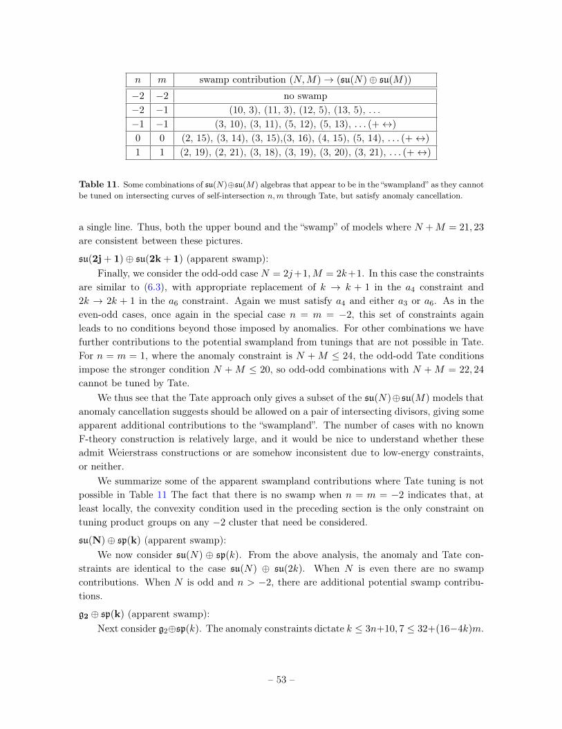
n m swamp contribution (N,M)→ (su(N)⊕ su(M))

−2 −2 no swamp−2 −1 (10, 3), (11, 3), (12, 5), (13, 5), . . .−1 −1 (3, 10), (3, 11), (5, 12), (5, 13), . . . (+↔)

0 0 (2, 15), (3, 14), (3, 15),(3, 16), (4, 15), (5, 14), . . . (+↔)

1 1 (2, 19), (2, 21), (3, 18), (3, 19), (3, 20), (3, 21), . . . (+↔)

Table 11. Some combinations of su(N)⊕su(M) algebras that appear to be in the “swampland” as they cannotbe tuned on intersecting curves of self-intersection n,m through Tate, but satisfy anomaly cancellation.

a single line. Thus, both the upper bound and the “swamp” of models where N +M = 21, 23

are consistent between these pictures.

su(2j + 1)⊕ su(2k + 1) (apparent swamp):Finally, we consider the odd-odd case N = 2j+1,M = 2k+1. In this case the constraints

are similar to (6.3), with appropriate replacement of k → k + 1 in the a4 constraint and2k → 2k + 1 in the a6 constraint. Again we must satisfy a4 and either a3 or a6. As in theeven-odd cases, once again in the special case n = m = −2, this set of constraints againleads to no conditions beyond those imposed by anomalies. For other combinations we havefurther contributions to the potential swampland from tunings that are not possible in Tate.For n = m = 1, where the anomaly constraint is N + M ≤ 24, the odd-odd Tate conditionsimpose the stronger condition N + M ≤ 20, so odd-odd combinations with N + M = 22, 24

cannot be tuned by Tate.We thus see that the Tate approach only gives a subset of the su(N)⊕su(M) models that

anomaly cancellation suggests should be allowed on a pair of intersecting divisors, giving someapparent additional contributions to the “swampland”. The number of cases with no knownF-theory construction is relatively large, and it would be nice to understand whether theseadmit Weierstrass constructions or are somehow inconsistent due to low-energy constraints,or neither.

We summarize some of the apparent swampland contributions where Tate tuning is notpossible in Table 11 The fact that there is no swamp when n = m = −2 indicates that, atleast locally, the convexity condition used in the preceding section is the only constraint ontuning product groups on any −2 cluster that need be considered.

su(N)⊕ sp(k) (apparent swamp):We now consider su(N) ⊕ sp(k). From the above analysis, the anomaly and Tate con-

straints are identical to the case su(N) ⊕ su(2k). When N is even there are no swampcontributions. When N is odd and n > −2, there are additional potential swamp contribu-tions.

g2 ⊕ sp(k) (apparent swamp):Next consider g2⊕sp(k). The anomaly constraints dictate k ≤ 3n+10, 7 ≤ 32+(16−4k)m.

– 53 –

The primary constraining Tate coefficient is again a4. To have a g2 on the n-curve, a4 musthave a coefficient proportional to z2. This imposes the constraint 2 ≤ 8+(4−k)m, equivalentto the second anomaly constraint. On the other hand, the Tate constraint on k is k ≤ 8 + 2n.For n = −2 this is equivalent to the anomaly constraint (k ≤ 4); for larger n, however, the Tateconstraint is stronger. There is also a further constraint from the condition that a6 must havea coefficient proportional to z3, or the g2 will be enhanced to so(7) or greater. This conditionimplies that 2k ≤ 12 + 3n, which is substantially stronger than the anomaly conditions. Forn = −2, we have k ≤ 3, for n = 1 we have k ≤ 4, for n = 0 we have k ≤ 6, etc.. Thus, there isan apparent tuning swampland of models that contains, for example, g2 ⊕ sp(4) when the g2

is on a −2 curve, and has four fundamental hypermultiplets. This is true in particular whenthe sp(n) factor is on a −1 curve, in which case this should be an SCFT, so this representsanother potential contribution to the 6D SCFT swampland. It is not clear whether there canor cannot be a Weierstrass model in this case as Weierstrass and Tate are not necessarilyequivalent for sp(4), though as mentioned earlier it seems likely that no non-Tate Weierstrassmodel can be realized for this algebra without involving exotic matter. Further elements ofthe swampland in this case include g2⊕sp(5) through g2⊕sp(7) when the g2 is on a −1 curve,g2 ⊕ sp(7) through g2 ⊕ sp(10) when the g2 is on a 0 curve, etc..

so(N)⊕ sp(k) (apparent swamp):

Finally, we turn to the cases so(N)⊕sp(k). These are the most delicate cases; we considerthe small values of N explicitly. We begin with so(8)⊕ sp(k). In this case, the three differenteight-dimensional representations 8v,8s,8c are equivalent under anomalies, and physicallyrelated through triality symmetry. Anomaly constraints limit k ≤ 4 + n, 2 ≤ 8 + (4 − k)m.For a Tate tuning the constraints associated with upper bounds on the size of the group are,similar to the g2 case, 2 ≤ 8 + (4− k)m, again like the second anomaly constraint, and againthe constraint k ≤ 8 + 2n which now matches the first anomaly constraint. So it seems thatthe anomaly and Tate constraints are consistent. There is however a subtlety here associatedwith the monodromy condition for so(8). This imposes the condition that the order z4 term ina2

2 − 4a4 must vanish [32]. In the special case that the sp(k) has k = 1, and n = −2, the onlypossible monomial in a4 of order w is wz2. But this cannot be part of a perfect square, so theso(8) monodromy condition cannot be satisfied. Thus, in this case the tuning is not possible.Furthermore, in this case even a Weierstrass tuning is not possible. This fact was mentionedin §5.1, and we elaborate further here. It was shown in [38] that so(8)⊕ su(2) = so(8)⊕ sp(1)

cannot be tuned on any pair of intersecting divisors where the second factor is realized througha Kodaira type III or IV singularity; the argument there was given in the context of threefoldbases, but holds for bases of any dimension. The argument given there shows in this contextthat in 6D, so(8) ⊕ su(2) cannot be tuned on any pair of intersecting divisors where thesecond divisor is a −2 curve. It was also shown in [19], in the context of 6D SCFTs, that anso(8) ⊕ su(2) cannot be realized on a pair of intersecting −3,−2 curves. The upshot of thisanalysis is that an su(2) on any −2 curve cannot intersect an so(8) on any divisor (not just

– 54 –

a −3 curve)10. This apparent element of the tuning swampland was shown to be inconsistentat the level of field theory in [60]; actually, the argument there demonstrated this resultonly at the superconformal point, but the same result should hold for a general 6D F-theorysupergravity model, since locally the −2 curve can generally be contracted to form an SCFT.This is an interesting example of a case where an apparent element of the tuning swamplandis removed by realization of a new field theory inconsistency.

We turn now to so(7) ⊕ sp(k). The anomaly constraints are similar but now depend onwhether the bi-charged matter is in the spinor (8s) or fundamental (7) representation. Inall cases, the second constraint 2 ≤ 8 + (4 − k)m agrees between anomalies and Tate. Theanomaly conditions for spinor matter are k ≤ 8+2n and for fundamental matter are k ≤ 3+n.Performing a generic Tate tuning, the bound is k ≤ 8 + 2n. This suggests that the generalTate tuning gives matter must be in the spinor-fundamental representation. This matches withthe known examples of the −2,−3,−2 non-Higgsable cluster, which carries spinor matter foran so(7) on the −3 curve, and the results of [60] that the four su(2) fundamental matterfields on an −2 curve transform in the spinor representation of an so(7) flavor group. Thatresult implies that for an su(2) on a −2 curve there cannot be a bifundamental with so(7),but a remaining open question is whether there can be an explicit Weierstrass tuning of anso(7) ⊕ sp(k) algebra on a more general pair of divisors with bifundamental matter, and ifthis is indeed impossible what the field theory reason is.

The other so(N)⊕sp(k) tunings can be analyzed in a similar fashion, though the analysisis simpler since anomalies show that spinors cannot appear at the intersection point. Forso(9) the Tate condition computed using the Tate form from Table 2 appears to give thebound k ≤ 6 + n from a6. This cannot be correct, since the anomaly bound gives k ≤ 5 + n,which seems to allow Tate constructions of models that violate anomaly cancellation. In fact,the maximal case k = 6 + n actually gives so(10). This can be understood if we carefullyimpose the proper additional monodromy condition. In terms of the Tate form of so(9) fromTable 2, the algebra is actually so(10) if (a2

3 + 4a6)/z4 is a single monomial when evaluated atz = 0, and thus a perfect square, which occurs for the generic Tate form in the current contextprecisely when k = 6 + n. So this Tate condition and the corresponding anomaly conditionfor so(9) match perfectly. The Tate bound on k from m, 4 ≤ 12 + (6− k)m, is stronger thanthe anomaly bound, 9 ≤ 32 + (16 − 4k)m, but both are satisfied for all compatible values ofm, k from §4.3.2, so there is no swampland.

For so(10), we can enforce the monodromy condition that (a23 + 4a6)/z4 is a perfect

square on z = 0 by setting a6 to vanish to order z5 instead of z4. In this class of tunings,the anomaly condition k ≤ 6 + n matches the a3 Tate condition k ≤ 6 + (3 − 2)n, while them condition 10 ≤ 32 + (16− 4k)m from anomalies is slightly weaker than the Tate condition2 ≤ 6 + (3 − k)m, leaving in the tuning swampland for example so(10) ⊕ sp(k) for k = 8, 9

when m = +1 (and necessarily n ≥ 2, 3). For so(11), the Tate condition without consideringmonodromy is k ≤ 8 + n, which is again weaker than the anomaly condition k ≤ 7 + n. The

10Thanks to Clay Cordova for discussions on this point

– 55 –

discrepancy can again be corrected by the monodromy condition that for Tate so(11) as intable 2, we have so(12) when (a2

4 − 4a2a6)/z6 is a perfect square on z = 0. This monodromycondition is stated in [32] for so(4n+4) with n ≥ 3, but the analysis here indicates that it mustalso hold at n = 2. With this monodromy, the first conditions agree; the other conditions,11 ≤ 32 + (16− 4k)m and 2 ≤ 8 + (4− k)m also agree. There is an exact matching betweenanomaly conditions and Tate conditions for the cases so(12).

For tunings of so(N) ⊕ sp(k) where the so(N) is on a m = −4 curve, there is no apriori upper bound on N , and the pattern continues in a similar way as for so(9)-so(12). Forso(N = 4j), the a4 Tate bounds k ≤ 8 + (4− j)m = N − 8, j ≤ 8 + (4− k)m precisely matchthe anomaly bounds. For so(N = 4j + 2), the a3 Tate bound k ≤ 6 + (3 − j)m = N − 8

matches the anomaly bound and j ≤ 6 + (3− k)m⇒ N ≤ 26 + (12− 4k)m is stronger thanthe anomaly bound N ≤ 32 + (16− 4k)m, leaving a small swampland contribution. Similarlyfor so(4j + 1), so(4j + 3) when the proper monodromy conditions are incorporated as forso(9), so(11). The upshot of this analysis is that so(N)⊕ sp(k) tunings have a few swamplandcontributions, but not many.

6.3 Multiple curves intersecting Σ

Having analyzed the combinations of algebras that can be tuned on a pair of intersectingcurves, we can consider the more general class of local constraints associated with a singlecurve Σ that supports a gauge algebra g, and which intersects k other curves Σi, i = 1, . . . , k,with each curve having a fixed self-intersection. In principle such geometries can be analyzedusing the same methods used in the preceding section for a pair of curves. A more generalstructure relevant for this analysis is related to the global symmetry of the field theory overthe curve Σ. Such global symmetries were recently analyzed in the context of 6D SCFTs in[64]. From the field theory point of view, the global symmetry can be determined by thenature of the matter transforming under g. For example, the fundamental representationsof su(N) are complex, and on a curve carrying M such representations, there is a globalsymmetry su(M) that rotates the representations among themselves. In general, the directsum of the algebras gi supported on the k curves Σi that intersect Σ must be a subalgebra ofthe global algebra of Σ. The global symmetries for curves of negative self intersection werecomputed in [64], and these are included in the Tables in the Appendix of information abouttunings of groups on curves of fixed self-intersection. A similar computation can be carriedout for curves of nonnegative self intersection; indeed, the computations in the precedingsection are closely related to the computation of the global symmetry, though for the globalsymmetry the constraint associated with the curve intersecting the desired curve would bedropped. Note that in [64], only global symmetries associated with generic intersections wereincorporated, more generally, for example, there could be a component of the global symmetrygroup associated with antisymmetric representations of su(N), which can appear in morecomplicated bi-charged matter configurations [35]. Note also that in considering situationswhere multiple curves intersect a given curve Σ that supports a gauge algebra g, the distinctionbetween different realizations of g, such as between type I2 and III, IV realizations of su(2),

– 56 –

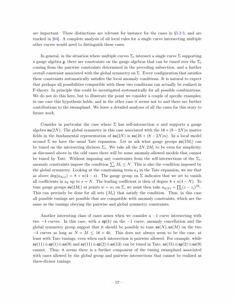
are important. These distinctions are relevant for instance for the cases in §5.2.3, and aretracked in [64]. A complete analysis of all local rules for a single curve intersecting multipleother curves would need to distinguish these cases.

In general, in the situation where multiple curves Σi intersect a single curve Σ supportinga gauge algebra g, there are constraints on the gauge algebras that can be tuned over the Σi

coming from the pairwise constraints determined in the preceding subsection, and a furtheroverall constraint associated with the global symmetry on Σ. Every configuration that satisfiesthese constraints automatically satisfies the local anomaly conditions. It is natural to expectthat perhaps all possibilities compatible with these two conditions can actually be realized inF-theory. In principle this could be investigated systematically for all possible combinations.We do not do this here, but to illustrate the point we consider a couple of specific examples;in one case this hypothesis holds, and in the other case it seems not to and there are furthercontributions to the swampland. We leave a detailed analyses of all the cases for this story tofuture work.

Consider in particular the case where Σ has self-intersection n and supports a gaugealgebra su(2N). The global symmetry in this case associated with the 16 + (8− 2N)n matterfields in the fundamental representation of su(2N) is su(16 + (8 − 2N)n). In a local modelaround Σ we have the usual Tate expansion. Let us ask what gauge groups su(2Mi) canbe tuned on the intersecting divisors Σi. We take all the 2N, 2Mi to be even for simplicity;as discussed above in the odd cases there will be some anomaly-allowed models that cannotbe tuned by Tate. Without imposing any constraints from the self-intersections of the Σi,anomaly constraints impose the condition

∑iMi ≤ N . This is also the condition imposed by

the global symmetry. Looking at the constraining term a4 in the Tate expansion, we see thatas above deg(a4(s)) = 8 + n(4 − s). The gauge group on Σ indicates that we set to vanishall coefficients in a4 up to s = N . The leading coefficient is then of degree 8 + n(4−N). Totune gauge groups su(2Mi) at points w = wi on Σ, we must then take a4(N) =

∏i(z − zi)Mi .

This can precisely be done for all sets {Mi} that satisfy the condition. Thus, in this caseall possible tunings are possible that are compatible with anomaly constraints, which are thesame as the tunings obeying the pairwise and global symmetry constraints.

Another interesting class of cases arises when we consider a −1 curve intersecting withtwo −4 curves. In this case, with a sp(k) on the −1 curve, anomaly cancellation and theglobal symmetry group suggest that it should be possible to tune so(N), so(M) on the two−4 curves as long as N + M ≤ 16 + 4k. This does not always seem to be the case, atleast with Tate tunings, even when each intersection is pairwise allowed. For example, whileso(11)⊕ sp(1)⊕ so(9) and so(11)⊕ sp(2)⊕ so(13) can be tuned in Tate, so(15)⊕ sp(2)⊕ so(9)

cannot. Thus, it seems there is a further component of the tuning swampland associatedwith cases allowed by the global group and pairwise intersections that cannot be realized asthree-divisor tunings.

– 57 –

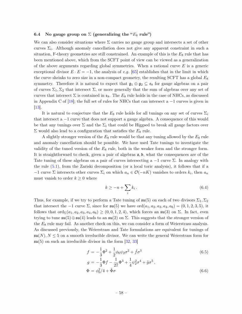
6.4 No gauge group on Σ (generalizing the “E8 rule”)

We can also consider situations where Σ carries no gauge group and intersects a set of othercurves Σi. Although anomaly cancellation does not give any apparent constraint in such asituation, F-theory geometries are still constrained. An example of this is the E8 rule that hasbeen mentioned above, which from the SCFT point of view can be viewed as a generalizationof the above arguments regarding global symmetries. When a rational curve E is a genericexceptional divisor E ·E = −1, the analysis of e.g. [65] establishes that in the limit in whichthe curve shrinks to zero size in a non-compact geometry, the resulting SCFT has a global E8

symmetry. Therefore it is natural to expect that g1 ⊕ g2 ⊆ e8 for gauge algebras on a pairof curves Σ1,Σ2 that intersect Σ, or more generally that the sum of algebras over any set ofcurves that intersect Σ is contained in e8. The E8 rule holds in the case of NHCs, as discussedin Appendix C of [18]; the full set of rules for NHCs that can intersect a −1 curves is given in[13].

It is natural to conjecture that the E8 rule holds for all tunings on any set of curves Σi

that intersect a −1 curve that does not support a gauge algebra. A consequence of this wouldbe that any tunings over Σ and the Σi that could be Higgsed to break all gauge factors overΣ would also lead to a configuration that satisfies the E8 rule.

A slightly stronger version of the E8 rule would be that any tuning allowed by the E8 ruleand anomaly cancellation should be possible. We have used Tate tunings to investigate thevalidity of the tuned version of the E8 rule, both in the weaker form and the stronger form.It is straightforward to check, given a pair of algebras a, b, what the consequences are of theTate tuning of these algebras on a pair of curves intersecting a −1 curve Σ. In analogy withthe rule (5.1), from the Zariski decomposition (or a local toric analysis), it follows that if a−1 curve Σ intersects other curves Σi on which an ∈ O(−nK) vanishes to orders ki, then anmust vanish to order k ≥ 0 where

k ≥ −n+∑i

ki . (6.4)

Thus, for example, if we try to perform a Tate tuning of su(5) on each of two divisors Σ1,Σ2

that intersect the −1 curve Σ, since for su(5) we have ord(a1, a2, a3, a4, a6) = (0, 1, 2, 3, 5), itfollows that ordΣ(a1, a2, a3, a4, a6) ≥ (0, 0, 1, 2, 4), which forces an su(3) on Σ. In fact, eventrying to tune su(5)⊕ su(4) leads to an su(2) on Σ. This suggests that the stronger version ofthe E8 rule may fail. As another check on this, we can consider a form of Weierstrass analysis.As discussed previously, the Weierstrass and Tate formulations are equivalent for tunings ofsu(N), N ≤ 5 on a smooth irreducible divisor. We can write the general Weierstrass form forsu(5) on such an irreducible divisor in the form [32, 33]

f = −1

3Φ2 +

1

2φ0ψ2σ

2 + fσ3 (6.5)

g = −1

3Φf − 1

27Φ3 +

1

4ψ2

2σ4 + gσ5 ,

Φ = φ20/4 + Φσ (6.6)

– 58 –

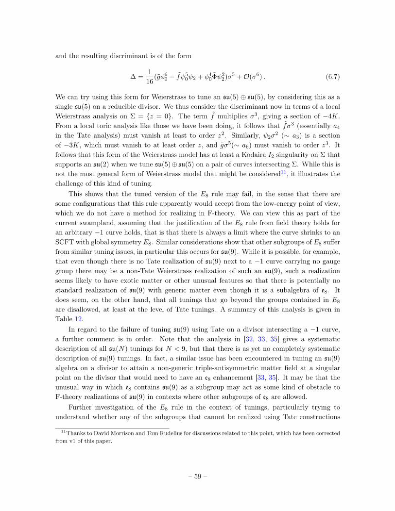
and the resulting discriminant is of the form

∆ =1

16(gφ6

0 − fψ50ψ2 + φ4

0Φψ22)σ5 +O(σ6) . (6.7)

We can try using this form for Weierstrass to tune an su(5)⊕ su(5), by considering this as asingle su(5) on a reducible divisor. We thus consider the discriminant now in terms of a localWeierstrass analysis on Σ = {z = 0}. The term f multiplies σ3, giving a section of −4K.From a local toric analysis like those we have been doing, it follows that fσ3 (essentially a4

in the Tate analysis) must vanish at least to order z2. Similarly, ψ2σ2 (∼ a3) is a section

of −3K, which must vanish to at least order z, and gσ5(∼ a6) must vanish to order z3. Itfollows that this form of the Weierstrass model has at least a Kodaira I2 singularity on Σ thatsupports an su(2) when we tune su(5)⊕ su(5) on a pair of curves intersecting Σ. While this isnot the most general form of Weierstrass model that might be considered11, it illustrates thechallenge of this kind of tuning.

This shows that the tuned version of the E8 rule may fail, in the sense that there aresome configurations that this rule apparently would accept from the low-energy point of view,which we do not have a method for realizing in F-theory. We can view this as part of thecurrent swampland, assuming that the justification of the E8 rule from field theory holds foran arbitrary −1 curve holds, that is that there is always a limit where the curve shrinks to anSCFT with global symmetry E8. Similar considerations show that other subgroups of E8 sufferfrom similar tuning issues, in particular this occurs for su(9). While it is possible, for example,that even though there is no Tate realization of su(9) next to a −1 curve carrying no gaugegroup there may be a non-Tate Weierstrass realization of such an su(9), such a realizationseems likely to have exotic matter or other unusual features so that there is potentially nostandard realization of su(9) with generic matter even though it is a subalgebra of e8. Itdoes seem, on the other hand, that all tunings that go beyond the groups contained in E8

are disallowed, at least at the level of Tate tunings. A summary of this analysis is given inTable 12.

In regard to the failure of tuning su(9) using Tate on a divisor intersecting a −1 curve,a further comment is in order. Note that the analysis in [32, 33, 35] gives a systematicdescription of all su(N) tunings for N < 9, but that there is as yet no completely systematicdescription of su(9) tunings. In fact, a similar issue has been encountered in tuning an su(9)

algebra on a divisor to attain a non-generic triple-antisymmetric matter field at a singularpoint on the divisor that would need to have an e8 enhancement [33, 35]. It may be that theunusual way in which e8 contains su(9) as a subgroup may act as some kind of obstacle toF-theory realizations of su(9) in contexts where other subgroups of e8 are allowed.

Further investigation of the E8 rule in the context of tunings, particularly trying tounderstand whether any of the subgroups that cannot be realized using Tate constructions

11Thanks to David Morrison and Tom Rudelius for discussions related to this point, which has been correctedfrom v1 of this paper.

– 59 –

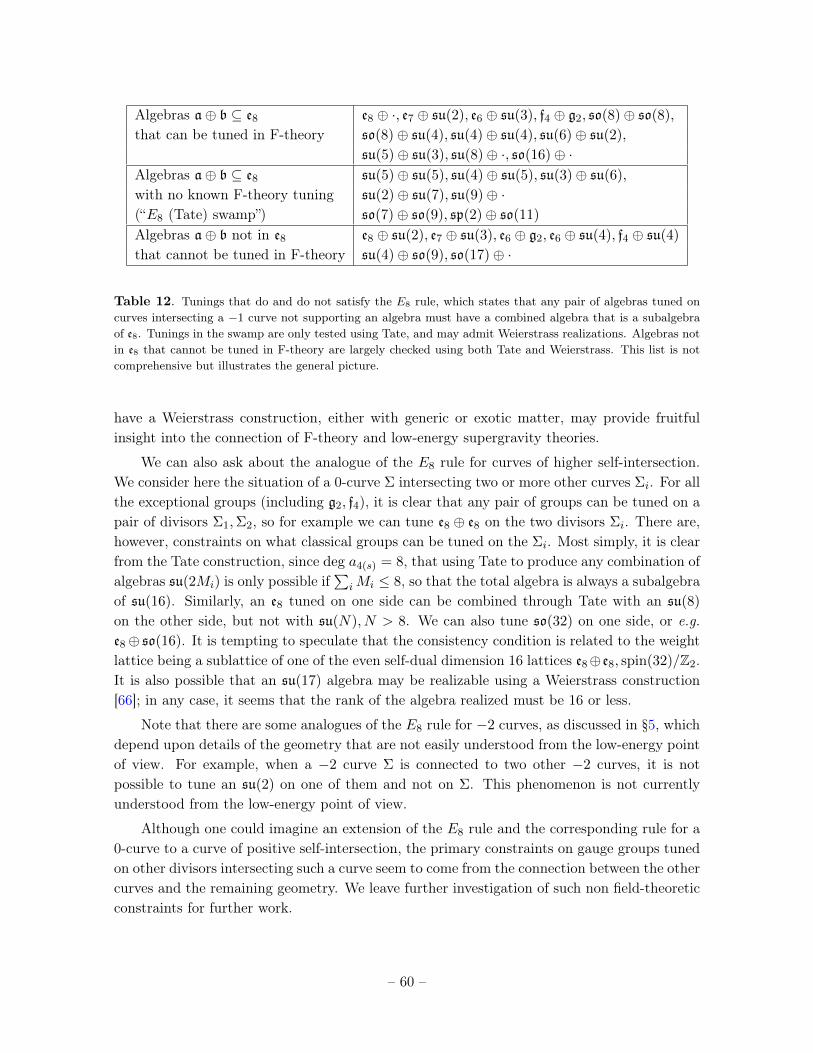
Algebras a⊕ b ⊆ e8 e8 ⊕ ·, e7 ⊕ su(2), e6 ⊕ su(3), f4 ⊕ g2, so(8)⊕ so(8),

that can be tuned in F-theory so(8)⊕ su(4), su(4)⊕ su(4), su(6)⊕ su(2),

su(5)⊕ su(3), su(8)⊕ ·, so(16)⊕ ·Algebras a⊕ b ⊆ e8 su(5)⊕ su(5), su(4)⊕ su(5), su(3)⊕ su(6),

with no known F-theory tuning su(2)⊕ su(7), su(9)⊕ ·(“E8 (Tate) swamp”) so(7)⊕ so(9), sp(2)⊕ so(11)

Algebras a⊕ b not in e8 e8 ⊕ su(2), e7 ⊕ su(3), e6 ⊕ g2, e6 ⊕ su(4), f4 ⊕ su(4)

that cannot be tuned in F-theory su(4)⊕ so(9), so(17)⊕ ·

Table 12. Tunings that do and do not satisfy the E8 rule, which states that any pair of algebras tuned oncurves intersecting a −1 curve not supporting an algebra must have a combined algebra that is a subalgebraof e8. Tunings in the swamp are only tested using Tate, and may admit Weierstrass realizations. Algebras notin e8 that cannot be tuned in F-theory are largely checked using both Tate and Weierstrass. This list is notcomprehensive but illustrates the general picture.

have a Weierstrass construction, either with generic or exotic matter, may provide fruitfulinsight into the connection of F-theory and low-energy supergravity theories.

We can also ask about the analogue of the E8 rule for curves of higher self-intersection.We consider here the situation of a 0-curve Σ intersecting two or more other curves Σi. For allthe exceptional groups (including g2, f4), it is clear that any pair of groups can be tuned on apair of divisors Σ1,Σ2, so for example we can tune e8 ⊕ e8 on the two divisors Σi. There are,however, constraints on what classical groups can be tuned on the Σi. Most simply, it is clearfrom the Tate construction, since deg a4(s) = 8, that using Tate to produce any combination ofalgebras su(2Mi) is only possible if

∑iMi ≤ 8, so that the total algebra is always a subalgebra

of su(16). Similarly, an e8 tuned on one side can be combined through Tate with an su(8)

on the other side, but not with su(N), N > 8. We can also tune so(32) on one side, or e.g.e8⊕ so(16). It is tempting to speculate that the consistency condition is related to the weightlattice being a sublattice of one of the even self-dual dimension 16 lattices e8⊕e8, spin(32)/Z2.It is also possible that an su(17) algebra may be realizable using a Weierstrass construction[66]; in any case, it seems that the rank of the algebra realized must be 16 or less.

Note that there are some analogues of the E8 rule for −2 curves, as discussed in §5, whichdepend upon details of the geometry that are not easily understood from the low-energy pointof view. For example, when a −2 curve Σ is connected to two other −2 curves, it is notpossible to tune an su(2) on one of them and not on Σ. This phenomenon is not currentlyunderstood from the low-energy point of view.

Although one could imagine an extension of the E8 rule and the corresponding rule for a0-curve to a curve of positive self-intersection, the primary constraints on gauge groups tunedon other divisors intersecting such a curve seem to come from the connection between the othercurves and the remaining geometry. We leave further investigation of such non field-theoreticconstraints for further work.

– 60 –

6.5 More general intersection structures

We have focused here on situations where multiple curves intersect a single curve Σ each at asingle point. More complicated possibilities can arise geometrically. For example, the curve Σ

can intersect itself at one or more points, or acquire a more complicated singularity. In suchsituations, a gauge group on Σ will either require an adjoint representation (when the tuningis in Tate form on a singular divisor) or a more exotic “higher genus” matter representationwhen the tuning is in non-Tate form; such configurations were discussed in §7.

Another interesting situation can arise when two curves Σ,Σ′ intersect at multiple points.In principle such geometries can be analyzed using similar methods to those used here. Wepoint out, however, one case of particular interest. If two −2 curves intersect at two points,or more generally if k −2 curves intersect mutually pairwise in a loop, then if we were to beable to tune an SU(N) group on each curve there would be bifundamental matter on eachpair of curves, and the shift in Hodge number h2,1(X) would be the same for every N . Thiswould appear to give rise to an infinite family of theories with a finite tuning. This example,along with a handful of other similar situations, was encountered in the low-energy theory in[67], and shown to be impossible in any supergravity theory with T < 9 in [41, 9]. Closedloops of this kind are also encountered in the context of F-theory realizations of little stringtheories [68]. From the F-theory point of view the possibility of an infinite family of tunings isincompatible with the proof of finiteness for Weierstrass models in [9]. We know, however, thatsuch −2 curve configurations are possible12, for example in certain rational elliptic surfacesthat can act as F-theory bases. In fact, these configurations are another example of degenerateelliptic curves, like those discussed in §5.2.2, but in this case associated with the affine Dynkindiagram Ak−1. As in those cases, we expect that the tuning of a single modulus will increaseN by one, and that there is an upper bound on N associated with the maximum value suchthat −12K − NΣ is effective. Note, however, that from the low-energy point of view thisconstraint is not understood. This issue is discussed further in §11.

Note that similar closed cycles of curves can occur for alternating −4,−1 sequences, withalternating SO(2k), Sp(k) gauge groups. These can be thought of as arising from blowing uppoints between every pair of −2 curves, and again correspond to degenerate genus one curveswith Σ · Σ = K · Σ = 0, and the explanation for finite tuning is again similar.

7 Tuning exotic matter

Up to this point we have focused on classifying the gauge groups that can be tuned over thevarious effective divisors in the base through tuning codimension one singularities in the Weier-strass model. In many circumstances, the gauge group content and associated Green-Schwarzterms, which are fixed by the divisors supporting the gauge group, uniquely determine thematter content of the theory. In other cases, however, there is some freedom in tuning codi-mension two singularities that can realize different anomaly-equivalent matter representations

12Thanks to Yinan Wang for discussions on this point

– 61 –

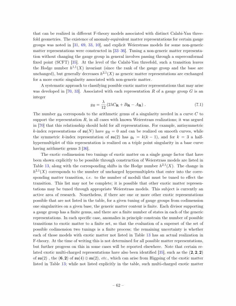
that can be realized in different F-theory models associated with distinct Calabi-Yau three-fold geometries. The existence of anomaly-equivalent matter representations for certain gaugegroups was noted in [31, 69, 33, 10], and explicit Weierstrass models for some non-genericmatter representations were constructed in [33–36]. Tuning a non-generic matter representa-tion without changing the gauge group in general involves passing through a superconformalfixed point (SCFT) [35]. At the level of the Calabi-Yau threefold, such a transition leavesthe Hodge number h1,1(X) invariant (since the rank of the gauge group and the base areunchanged), but generally decreases h2,1(X) as generic matter representations are exchangedfor a more exotic singularity associated with non-generic matter.

A systematic approach to classifying possible exotic matter representations that may arisewas developed in [70, 33]. Associated with each representation R of a gauge group G is aninteger

gR =λ

12(2λCR +BR −AR) . (7.1)

The number gR corresponds to the arithmetic genus of a singularity needed in a curve C tosupport the representation R, in all cases with known Weierstrass realizations; it was arguedin [70] that this relationship should hold for all representations. For example, antisymmetrick-index representations of su(N) have gR = 0 and can be realized on smooth curves, whilethe symmetric k-index representation of su(2) has gk = k(k − 1), and for k = 3 a half-hypermultiplet of this representation is realized on a triple point singularity in a base curvehaving arithmetic genus 3 [36].

The exotic codimension two tunings of exotic matter on a single gauge factor that havebeen shown explicitly to be possible through construction of Weierstrass models are listed inTable 13, along with the corresponding shifts in the Hodge number h2,1(X). The change inh2,1(X) corresponds to the number of uncharged hypermultiplets that enter into the corre-sponding matter transition, i.e. to the number of moduli that must be tuned to effect thetransition. This list may not be complete; it is possible that other exotic matter represen-tations may be tuned through appropriate Weierstrass models. This subject is currently anactive area of research. Nonetheless, if there are one or more other exotic representationspossible that are not listed in the table, for a given tuning of gauge groups from codimensionone singularities on a given base, the generic matter content is finite. Each divisor supportinga gauge group has a finite genus, and there are a finite number of states in each of the genericrepresentations. In each specific case, anomalies in principle constrain the number of possibletransitions to exotic matter to a finite set, so that the evaluation of a superset of the set ofpossible codimension two tunings is a finite process; the remaining uncertainty is whethereach of those models with exotic matter not listed in Table 13 has an actual realization inF-theory. At the time of writing this is not determined for all possible matter representations,but further progress on this in some cases will be reported elsewhere. Note that certain re-lated exotic multi-charged representations have also been identified [35], such as the (2,2,2)

of su(2) , the (6,2) of su(4)⊕ su(2), etc., which can arise from Higgsing of the exotic matterlisted in Table 13; while not listed explicitly in the table, such multi-charged exotic matter

– 62 –

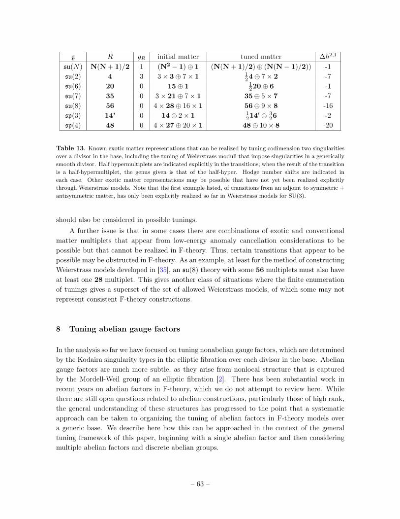
g R gR initial matter tuned matter ∆h2,1

su(N) N(N + 1)/2 1 (N2 − 1)⊕ 1 (N(N + 1)/2)⊕ (N(N− 1)/2)) -1su(2) 4 3 3× 3⊕ 7× 1 1

24⊕ 7× 2 -7su(6) 20 0 15⊕ 1 1

220⊕ 6 -1su(7) 35 0 3× 21⊕ 7× 1 35⊕ 5× 7 -7su(8) 56 0 4× 28⊕ 16× 1 56⊕ 9× 8 -16sp(3) 14’ 0 14⊕ 2× 1 1

214′ ⊕ 3

26 -2sp(4) 48 0 4× 27⊕ 20× 1 48⊕ 10× 8 -20

Table 13. Known exotic matter representations that can be realized by tuning codimension two singularitiesover a divisor in the base, including the tuning of Weierstrass moduli that impose singularities in a genericallysmooth divisor. Half hypermultiplets are indicated explicitly in the transitions; when the result of the transitionis a half-hypermultiplet, the genus given is that of the half-hyper. Hodge number shifts are indicated ineach case. Other exotic matter representations may be possible that have not yet been realized explicitlythrough Weierstrass models. Note that the first example listed, of transitions from an adjoint to symmetric +antisymmetric matter, has only been explicitly realized so far in Weierstrass models for SU(3).

should also be considered in possible tunings.A further issue is that in some cases there are combinations of exotic and conventional

matter multiplets that appear from low-energy anomaly cancellation considerations to bepossible but that cannot be realized in F-theory. Thus, certain transitions that appear to bepossible may be obstructed in F-theory. As an example, at least for the method of constructingWeierstrass models developed in [35], an su(8) theory with some 56 multiplets must also haveat least one 28 multiplet. This gives another class of situations where the finite enumerationof tunings gives a superset of the set of allowed Weierstrass models, of which some may notrepresent consistent F-theory constructions.

8 Tuning abelian gauge factors

In the analysis so far we have focused on tuning nonabelian gauge factors, which are determinedby the Kodaira singularity types in the elliptic fibration over each divisor in the base. Abeliangauge factors are much more subtle, as they arise from nonlocal structure that is capturedby the Mordell-Weil group of an elliptic fibration [2]. There has been substantial work inrecent years on abelian factors in F-theory, which we do not attempt to review here. Whilethere are still open questions related to abelian constructions, particularly those of high rank,the general understanding of these structures has progressed to the point that a systematicapproach can be taken to organizing the tuning of abelian factors in F-theory models overa generic base. We describe here how this can be approached in the context of the generaltuning framework of this paper, beginning with a single abelian factor and then consideringmultiple abelian factors and discrete abelian groups.

– 63 –

8.1 Single abelian factors

A general form for a Weierstrass model with rank one Mordell-Weil group, corresponding toa single U(1) factor, was described by Morrison and Park [71]. Over a generic base, such aWeierstrass model takes the form

y2 = x3 + (e1e3 −1

3e2

2 − b2e0)x+ (−e0e23 +

1

3e1e2e3 −

2

27e3

2 +2

3b2e0e2 −

1

4b2e2

1) . (8.1)

Here, b is a section of a line bundle O(L), where L is effective, and ei are sections of linebundles O((i − 4)K + (i − 2)L), where K is the canonical class of the base. This provides ageneral approach to tuning a Weierstrass model with a single U(1) factor. One chooses thedivisor class L, and then curves b, ei in the corresponding classes, which define the Weierstrassmodel.

A simple conceptual way of understanding this construction and the associated spectrumcomes from the observation, developed in [71, 72] (see also [73, 74]), that when b → 0 (8.1)becomes the generic form of a Weierstrass model from the SU(2) Tate form, where e3 isthe divisor supporting the SU(2) gauge group. The divisor class [e3] = −K + L alwayshas positive genus, since L is effective. Thus, the resulting SU(2) group has some adjointrepresentations. The U(1) model (8.1) can be found as the Higgsing of the SU(2) model onan adjoint representation, and has the corresponding spectrum. While in some situationsthe enhanced SU(2) leads to a singular F-theory model, the spectrum can still be analyzedconsistently from this point of view.

Thus, the generic tuning of a U(1) factor on an arbitrary base can be carried out bychoosing a curve e3 of genus g > 0. From Table 7, and the usual rules of Higgsing an SU(2)to a U(1), we see that the resulting matter spectrum consists of

generic U(1) : matter = (6n+ 16− 16g)(±1) + (g − 1)(±2) (8.2)

where n = [e3] · [e3] is the self-intersection of the curve e3. Since the Higgsing introduces oneadditional modulus for each uncharged scalar, the change in Hodge numbers for this tuningis g less than that for the SU(2) model:

generic U(1) : ∆(h1,1, h2,1) = (1,−12n+ 30(g − 1) + 1) . (8.3)

As the simplest example, choosing e3 to be a cubic on P2 with n = 9 gives g = 1, and a mattercontent of 108 fields of charge ±1 under the U(1), while the Hodge numbers are (3, 166). Notethat here the Hodge number h2,1(X) is determined from the low-energy theory using the rulesof Higgsing and anomaly cancellation; directly computing the number of independent moduliin the Weierstrass model (8.1) is tricky due to possible redundancies, and has not yet beencarried out in general, to the best knowledge of the authors.

This approach allows for the tuning of a generic U(1) on an arbitrary base. The spectrumwill become more complicated when e3 intersects other divisors that carry gauge groups, andmust be analyzed in a parallel fashion to other intersecting divisors that each carry nonabelian

– 64 –

gauge factors. A recent systematic analysis of this type, for example, was carried out in [75].When the U(1) derives from the Higgsing of an SU(2), however, the matter follows directlyfrom the Higgsing process and can be tracked in the low-energy theory. Note also that thecurve e3 can be reducible, in which case the corresponding SU(2) model will arise on a productof irreducible factors, with bifundamental matter in place of adjoint matter; such situationsare discussed in some detail in [34].

The U(1) factors tuned in this way will have only the generic types of U(1) matter,associated with charges q = ±1,±2. It is known, however, that U(1) models with highercharges such as q = ±3 can be found, see e.g. [73]. As described in [36], such U(1) modelscan be described as arising from the Higgsing of SU(2) models with exotic matter, such as inthe three-index symmetric matter representation. From the point of view of the unHiggsednonabelian model, the SU(2) factor on e3 can acquire exotic matter through a transition suchas the one described in the second line of Table 13 where 3 adjoints of SU(2) and seven neutralfields are exchanged for a half-hypermultiplet in the 4 representation and seven fundamentals,with a shift in h2,1 of -7. If the resulting theory has at least one further adjoint, on whichthe SU(2) is then Higgsed, this gives a U(1) factor with charge q = ±3. By systematicallyconstructing all SU(2) models with exotic matter we thus should in principle be able toconstruct all U(1) models with higher charges. There are a number of questions here thatare still open for further work, however. We summarize the situation briefly. As discussed in[72], when the U(1) is unHiggsed to SU(2) it may introduce (4, 6) singularities at codimensiontwo or even at codimension one. Thus, a systematic analysis of all U(1) models with exoticmatter through Higgsing might require constructing classes of singular SU(2) models. A moredirect approach would be to consider how the SU(2) transition to exotic matter is inherited inthe U(1) theory, where it should correspond to a direct transition of U(1) models exchangingstandard matter types for q = ±3 or higher matter. From the general analysis of [35], suchabelian transitions should pass through superconformal fixed points of the theory. A directconstruction of these transitions in the U(1) theory has not yet been completed. It is alsonot known in principle whether all U(1) models with charge 3 matter can be constructed inthis fashion through Higgsing of models with the same or higher rank nonabelian symmetry.Further work is thus needed to complete the classification of non-generic F-theory modelswith a single U(1) factor and higher charged matter over a given base. One way to frame thisquestion is in the context of 6D string universality [23]; from the low-energy point of view,for a given gauge group and associated divisor class, we can classify the finite set of matterrepresentations that are in principle allowed. For a theory with abelian factors, some progresswas made in classifying the allowed spectra in [40, 76, 77], but a complete classification hasnot been made. The open question is whether in all cases with abelian factors, all anomaly-allowed matter representations can be realized by explicit Weierstrass models in F-theory. Inparticular, for generic SU(2) models with 4 or higher matter or the corresponding HiggsedU(1) models with matter of charges q = ±3 or higher, while some F-theory examples havebeen constructed others have not, and the universality question is still open.

– 65 –

8.2 Multiple U(1)’s

As the rank of the abelian group rises, the algebraic complexity of explicit constructionsincreases substantially. A general rank two U(1) × U(1) Weierstrass model was constructedin [34] (less general U(1)2 models were constructed in [78–83]). The general U(1)2 model canbe understood in a similar fashion to the U(1) models just described, in terms of unHiggsingto a nonabelian model. In general, there is a divisor class associated with each U(1) factor;most generally, these divisor classes can be reducible, and there may be some overlap betweenthe curves supporting the resulting SU(2) factors, in which case the rank is increased to twoover the common divisor. Specifically, if we denote by AC,BC the curves on which the“horizontal” U(1) divisors become vertical, with C the common factor, as described in [34],the unHiggsed gauge group will be SU(2) × SU(2) × SU(3), with the factors supported oncurves A,B,C, each of which may be further reducible in which case the gauge group acquiresmultiple factors accordingly. The charges of the general U(1) × U(1) model can then beunderstood simply from the Higgsing of the appropriate nonabelian model, in parallel to theconstruction described above for a single U(1) factor from the unHiggsed SU(2) spectrum.The details become somewhat more complicated, and we do not go into them explicitly here(see [34]), but the tuning and full spectra of a generic U(1) × U(1) model can in principle bedescribed using this analysis.

As in the case of a single U(1), the generic U(1) × U(1) spectrum described here consistsof only the most generic types of charged matter under the two abelian factors. Note, however,that this includes matter charges associated with a symmetric representation of SU(3), whichcan be realized for example, from the Higgsing of an SU(3) on a singular curve with doublepoint singularities and a non-Tate model with a symmetric representation and at least oneadditional adjoint, as constructed in [34, 35]. For more exotic matter representations, thereis as yet no general understanding, and many of the open questions described above, suchas the explicit realization of abelian matter transitions, and the existence and Higgsing ofappropriate rank two nonabelian models with exotic matter, are relevant here as well.

Constructing models with more U(1)’s becomes progressively more difficult. One classof U(1)3 models was constructed in [84], though these models do not capture many of thespectra that could result from Higgsing nonabelian rank 3 models, and are certainly notgeneral. The construction of a completely general abelian model with U(1)k where k > 2 isstill an open problem. Nonetheless, from the point of view of geometry and field theory ageneral approach was outlined in [34] that in principle gives an approach to the tunings thatgives what should be a superset of the set of allowed possibilities, in the spirit of this paper.The idea is that each U(1) factor should come from a divisor Ci, and these divisors can bereducible, with separate components in principle for each subset of the divisors, generalizingthe AC,BC rank two construction described above. To proceed then, we consider all possibledivisor combinations that can support an unHiggsed rank k nonabelian group. The possiblerank k abelian group constructions, and the corresponding charges, can then be determinedfrom Higgsing the corresponding nonabelian model. In each case, the specific spectrum and

– 66 –

anomaly cancellation conditions allow us to compute the potential shift in Hodge numbers.This gives in principle a finite list of possibilities that would need to be checked for theexistence of an explicit Weierstrass model. In practice, the fact that no generic way is knownto implement Higgsing in the Weierstrass context makes the explicit check impossible withcurrent technology, even for generic types of matter. Here we also in principle would need todeal with exotic matter contents.

Another approach to constructing higher-rank abelian models proceeds through construct-ing fibrations with particular special fiber types that automatically enhance the Mordell-Weilrank, see e.g. [85, 73]. It is not clear, however, how this approach can be used in the systematicconstruction of models, particularly through the perspective of tuned Weierstrass models as wehave considered here. Nonetheless, this approach may provide a useful alternative perspectiveon the systematic construction of higher-rank abelian theories.

To summarize, for rank one U(1) models with generic matter, we have a systematicapproach to constructing all tunings. When considering more exotic matter or higher ranknonabelian groups, we have a systematic algorithm for constructing a finite set of possibilitiesalong with the Hodge numbers of the elliptic Calabi-Yau threefold, but the technology doesnot yet exist to explicitly check all possibilities. Note that there is also as yet no proof thatthe general higher rank Higgsing strategy will give all possible higher-rank abelian spectra,unlike for rank one and two with generic matter, where the results of [71, 34] represent generalconstructions, all of which are compatible with the Higgsing approach.

8.3 Discrete abelian gauge factors

Finally, we describe briefly the possibility of systematic tunings of discrete abelian gaugefactors. Such discrete factors, and corresponding matter, have been the subject of substantialrecent work [72, 86–93]. As described in [72], one systematic way to approach discrete abelianfactors is through the Higgsing of continuous abelian U(1) factors on states of higher charge.For example, Higgsing a U(1) theory with matter of charge ±1 on a field of charge +2 givesa theory with a discrete abelian Z2 symmetry and matter of charge 1 under the Z2. In thecontext of (8.1), this Higgsing can be realized by transforming b2 into a generic section e4 ofthe line bundle O(2L). This gives an explicit approach to constructing the simplest class ofdiscrete abelian gauge models, those with Z2 gauge group and charges 1. On a generic base,choosing e3 to be a curve of genus g and self-intersection n, the resulting spectrum and Hodgeshifts should be

generic Z2 : matter = (6n+ 16− 16g)(±1), ∆(h1,1, h2,1) = (0,−12n+ 32(g − 1)) . (8.4)

A construction of a theory with a discrete abelian Z3 symmetry from a U(1) factor with matterof charge q = ±3 was given in [91]. While constructions of models with more complicatedgroups and/or matter over generic bases have not been given explicitly in full generality, wecan follow the same approach as used for the general U(1)k models to construct a class ofpotential Hodge numbers and spectra that should be a superset of the set of allowed F-theory

– 67 –

possibilities. Basically, for each possible U(1)k model, we consider the Higgsings on chargedmatter that leave a residual discrete gauge group. In addition to the caveats discussed abovefor the U(1)k models, there are also the issues that the U(1)k model may in principle besingular even if the model with the discrete symmetry is not, and that in principle there maybe allowed models with discrete symmetries that cannot be lifted to U(1)k models. These areall good open questions for further research that would need to be resolved to complete theclassification process in this direction.

9 A tuning algorithm

We now describe a general algorithm that, given any explicit choice of base B, produces a finitelist of possibilities for tuned Weierstrass models. In the most concrete case of toric bases andtunings over toric divisors, this algorithm can be carried out in an explicit way to enumerateand check all possibilities. More generally, the algorithm will produce a superset of possibletunings, for which explicit realizations as Weierstrass models must be confirmed. We beginby describing the algorithm in a step-by-step fashion. We then summarize the outstandingissues related to this algorithm.

9.1 The algorithm

i) Choose a baseWe begin by picking a complex surface base that supports an elliptically fibered Calabi-

Yau threefold. As summarized earlier, from the work of Grassi [21] and the minimal modelprogram, this surface must be a blow-up of P2 or a Hirzebruch surface Fm,m ≤ 12. TheEnriques surface can also be used as a base, but the canonical class is trivial up to torsion, sof, g do not seem to have interesting tunings. The important data on the base that must begiven includes the Mori cone of effective divisors and the intersection form.

ii)Tune nonabelian groups with generic matter on effective divisors of self-intersection≤ −1

The set of effective irreducible curves of negative self-intersection forms a connected set.This can be seen inductively: The statement certainly holds for all the Hirzebruch surfaces Fm;for m > 0, Fm contains a single curve of negative self-intersection, and for m = 0 there are nosuch curves. And any point p in a Hirzebruch surface, or any blow-up thereof, either lies on acurve of negative self-intersection, or on a fiber of the original Hirzebruch with self-intersection0, so blowing up p gives another base with the desired property. (In the latter case, the fiberbecomes a −1 curve after the blow-up, which intersects the negative self-intersection curve onthe original Fm.)

Furthermore, at least one curve of negative self-intersection in any base containing suchcurves will intersect an effective curve of self-intersection 0. This can be seen by taking, forexample the original −m curve on any blow-up of Fm, m > 0, and noting that any base otherthan P2 and F0 can be seen as a blow-up of Fm,m > 0.

– 68 –

Together, these statements and our analysis of §4, §6.2 are sufficient to prove that inprinciple there are a finite number of possible tunings on all curves of negative self-intersectionas long as the Mori cone contains a finite number of generators. We can proceed by startingwith a negative self-intersection curve Σ that intersects a 0-curve, construct the finite setof possible tunings over Σ, etc., and then proceed by constructing tunings over curves thatintersect that curve, etc., checking consistency with previous curves at each stage. This showsin principle that there is a finite algorithm for constructing all tunings over curves of negativeself-intersection given a finitely generated Mori cone.

Note that the Mori cone contains a finite number of curves of self-intersection −2 or below.In practice, we can proceed effectively by using the results of Section 4, 5 to construct allpossible tunings of nonabelian gauge groups on individual effective divisors and non-Higgsableclusters represented by curves of self-intersection −2 or below as units in the algorithm. Theconnection with −1 curves and at least one 0-curve are needed in principle to bound the infinitefamilies that otherwise could be tuned on chains of −2 curves or alternating −4,−1,−4,−1, . . .

chains, and are also useful in practice to bound the exponential complexity that would beencountered by independently tuning the clusters without consideration of their connections.

Note also that in some unusual cases like dP9, the Mori cone has an infinite numberof generators, associated with an infinite number of (−1)-curves. This algorithm appearsinadequate in such cases, however in all cases that we are aware of of this type, nothing canbe tuned on the infinite family of −1 curves due to a low number of available moduli in h2,1.This issue is discussed further below.

iii) Tune nonabelian groups on the remaining effective divisors

We now consider tunings on remaining effective curves of non-negative self-intersection.We restrict attention to cases where the number of generators of the Mori cone is finite, andthere are a finite number of effective curves with genus below any fixed bound; we discussbelow situations where the number of Mori generators is infinite. The effective curves onwhich gauge groups can be tuned are generally quite constrained. From the analysis of §6.1,no gauge group can be tuned on any divisor that intersects a curve on which an algebra off4 or above is supported. Thus, the non-negative curves on which we are allowed to tune areperpendicular to all such curves, in particular perpendicular to all curves of self-intersection−5 or below. This acts as a powerful constraint, particularly for bases with large h1,1(B),which can only arise in the presence of many curves that have large non-Higgsable gaugefactors. An example is given in §10.2. Restricting attention to curves C in the subspace withC ·D = 0 for all D of self-intersection D ·D ≤ −5, the genus grows as g = 1 + (K +C) ·C/2,which increases rapidly with the self-intersection of C. Practically, this rapidly bounds theset of curves on which tunings are possible. While we do not give here an explicit algorithmfor efficiently enumerating these curves, in general, the finiteness of the number of tuningsfollows from an argument given in [9], which uses the Hilbert Basis Theorem to show that thenumber of distinct strata of tuning in the moduli space of Weierstrass models is finite. Wenow can in principle consider all possible tunings of the divisors that admit tunings (using

– 69 –

Tables 4 and 7), and constrain using the rules that govern connected divisors described inSection 6. This gives a finite list of possible nonabelian gauge factors tuned on divisors in thebase, which by construction satisfy the 6D anomaly cancellation conditions.

iv) Tune abelian gauge factorsWe can use the methods described in Section 8 to identify the set of possible abelian models

and spectra that could in principle be realized from the Higgsing of additional nonabeliangauge factors on effective divisors.

v) Tune exotic matterFinally, we can, in any specific case, identify a finite number of possible tunings to

anomaly-equivalent exotic matter content, as described in Section 7. Table 13 gives the setof possible such transitions that have been explicitly identified in Weierstrass models. Thisgives a finite set of possible matter contents for a given nonabelian gauge content, thoughas discussed earlier not all of these may have Weierstrass realizations. Analogous transitionscan be carried out for abelian factors, either through the corresponding unHiggsed nonabeliantheory, or in principle directly through abelian matter transitions.

9.2 Open questions related to the classification algorithm

Here we summarize places where the algorithm encounters issues that are not yet resolved.Each of these is an interesting open research problem. Note that for tunings of nonabeliangauge groups with generic matter over toric divisors in toric bases, there are no outstandingissues, and the algorithm can in principle be carried out for all bases and tunings.• Base issues

The algorithm described here requires that the cone of effective divisors on the base havea finite number of generators. This is not the case for some special cases of bases such as the9th del Pezzo surface dP9. The algorithm described here would not work for such bases. Whilethe algorithm described here can be carried out for any specific base with a finitely generatedcone of effective divisors, the full program of classifying all elliptic Calabi-Yau threefolds alsorequires classifying the set of allowed bases. In [16], all non-toric bases that support ellipticCalabi-Yau threefolds with h2,1 ≥ 150 were constructed (these all have finitely generated Moricones, so the algorithm here could be applied without encountering this problem in classifyingall tuned elliptic Calabi-Yau threefolds with h2,1 ≥ 150). To continue the algorithm usedthere to arbitrarily low Hodge numbers would require resolving several issues in addition tothe finite cone issue. In particular, that algorithm used the intersection structure of classesin the Mori cone. In some cases at lower Hodge numbers this does not uniquely fix theintersection structure of effective divisors on the base; for example, one must distinguish caseswhere 3 curves intersect one another in pairs from the case where all three intersect at a point.

• Apparent infinite families

– 70 –

As mentioned above, in some bases such as dP9 the Mori cone has an infinite number of −1

curves. Our algorithm would appear to break down in such situations. Because the numberof tunings is proven to be finite, however, there cannot be any tunings on an infinite family ofdistinct curves. Thus, it seems that the finite number of moduli in any given case must limitthe possibilities so that there are nonetheless a finite number of tunings. For example, for thebase dP9 we have H = 273 − 29 · 9 = 12, giving insufficient moduli to tune even an SU(2)on a −1 curve, so in fact the number of tunings here is finite even though the number of −1

curves is infinite.We have also not given a completely rigorous proof and explicit algorithm for enumerating

the set of curves of self-intersection 0 or above on a base with a finitely generated Moricone. While we believe that this is in principle possible, and in explicit examples seemsstraightforward, a more general analysis and explicit algorithm relevant for non-toric baseswould be desirable.

• Explicit Weierstrass tuningsIn the work here we have carried out local analyses that ensure the existence of Weier-

strass models for any of the local tunings over individual curves or clusters of curves of self-intersection -2 or below, except some cases of large rank classical groups or complicated -2curve structures. Beyond these cases, we have used anomaly cancellation conditions to de-termine a superset of the set of allowed models for tunings over general local configurationsof arbitrary curves, with Tate models used to produce most allowed constructions in the caseof intersecting rational curves. An explicit implementation of the algorithm would need toconfirm the existence of Weierstrass models to determine which models in the superset admitexplicit constructions. We are not aware of any known exceptions to the existence of Weier-strass models other than those discussed explicitly here, but we cannot rule them out forexample when considering multiple intersecting curves supporting nonabelian gauge groups,or gauge groups on higher genus curves.

• Exotic matter representationsWe have listed in Table 13 the set of non-generic matter representations that have been

found identified in the literature through explicit Weierstrass models. Even for these matterrepresentations, it is not clear whether all combinations of fields that satisfy anomaly can-cellation can be realized in F-theory constructions. It is also not known whether there areother exotic matter representations that may admit realizations in F-theory. We have alsoassumed that all exotic matter representations can be realized through a transition from ananomaly-equivalent set of generic representations; this statement is not proven.

• Codimension two resolutionsAs mentioned in §2.5, while our algorithm in principle could hope to classify the complete

finite set of Weierstrass models over a given base, there is a further challenge in finding allresolutions of the Weierstrass model to a smooth elliptic Calabi-Yau threefold. Despite therecent work on codimension two resolutions in the F-theory context [33, 51–56], there is as yetno general understanding or systematic procedure for describing such resolutions, particularly

– 71 –

in the context of the exotic matter representations just mentioned where the curve in the basesupporting a nontrivial Kodaira singularity is itself singular. While the number of distinctWeierstrass models must be finite by the argument of [9], to the best of our knowledge thereis no argument known that the number of distinct resolutions of codimension two singularitiesin a given Weierstrass model is finite 13, so a complete classification of elliptic Calabi-Yauthreefolds would require further progress in this direction.

• Abelian gauge groupsWe have outlined an approach to constructing a superset of the set of possible abelian

models over a given base. For a single U(1) and generic (charge 1, 2) matter, this can be donevery explicitly using the Morrison-Park form [71] and Higgsing of SU(2) models on highergenus curves. For two U(1) factors and generic matter this can in principle similarly be donefollowing the analysis of [34], though we have not gone through the details of the possibilitieshere. For more U(1) factors, while the approach described here and in [34] can in principle givea finite set of abelian models through Higgsing nonabelian models, which should represent asuperset of the set of allowed possibilities, there is no general construction known of the explicitmultiple U(1) models. For non-generic U(1) charged matter, again while in principle a finitelist of possibilities compatible with anomaly cancellation can be made, explicit Weierstrassconstructions beyond those of charge 3 matter in [36] are not known. In principle, exoticmatter transitions could be classified directly in terms of the abelian spectrum, though thishas not yet been done. For discrete abelian groups, again in principle a finite set of possibilitiescan be constructed by Higgsing the abelian models, but explicit Weierstrass constructions arenot known beyond the generic Z2 models and some Z3 models mentioned above.

Most of the complications and issues that arise in confirming the existence of Weierstrassmodels for complicated gauge-matter combinations arise only as the Hodge number h2,1(X)

becomes small. None of these issues were relevant in the classification of Weierstrass modelsfor elliptic Calabi-Yau threefolds with h2,1 ≥ 350 in [17], and we expect that one could go quitea bit further down in h2,1 before encountering a problem with the systematic classificationthat would require substantially new insights into any of these problems.

We also emphasize that in principle, there is no obstruction to carrying out this algorithmfor arbitrary toric constructions, with nonabelian gauge tunings only over toric divisors.

10 Examples

In this section we give some examples of applications of the methods developed and describedhere. In each case, the goal is not to be comprehensive, but to illustrate the utility of themethodology developed in this paper and to suggest directions for more comprehensive futurework.

13Thanks to D. Morrison for discussions on this point

– 72 –

10.1 Example: two classes of tuned elliptic fibrations in Kreuzer-Skarke

The rules that we have established so far must in particular be satisfied by any Calabi-Yauelliptic fibration over toric surfaces. We have a complete set of rules that list the allowedtunings on isolated toric curves; on multiple-curve NHCs; and on clusters either neighboringor separated by a −1 curve. In each case we have provided a formula for the shift in Hodgenumbers of the resulting threefold in comparison to a general elliptically fibered Calabi-Yauover the same base. It is perhaps useful at this point to see how these rules simplify practicalcomputations.

To this end, we use our rules to explore two classes of tuned fibrations within the Kreuzer-Skarke database [58], which contains all Calabi-Yau threefolds that can be realized as hyper-surfaces in toric varieties associated with reflexive 4D polytopes. In the future, these rulesmay be useful to perform a more exhaustive study of all tuned elliptic fibrations over toric(or more general) surfaces. For purposes of illustration, we will consider the following simpleclasses of fibrations over toric bases as classified in [14]:

• tunings of e6, e7 over −4 curves.14

• tunings of su(2) over −2 curves.

Proceeding to the first example, whenever a base contains a −4 curve, we enhance itsgeneric so(8) to e6 and e7 when possible. By the E8 rule, this will be possible whenever theneighboring clusters (separated by −1 curves) support at most su(3) or su(2) algebras, respec-tively. For instance, the −4 curve in the sequence (· · · ,−3,−2,−1,−4,−1−2,−3, · · · ) will ad-mit enhancement to e7, whereas the−4 curve in the sequence (· · · ,−1,−3,−1,−4,−1,−3,−1, · · · )will admit an enhancement only to e6, and no enhancement is possible on(· · · ,−2,−3,−1,−4,−1,−3,−2,−1, · · · ), since the −3 curve of a (−3,−2) NHC supports thealgebra g2 and g2 ⊕ e6 * e8.

Implementing this program yields the following results, as plotted in the diagram below.There are 1, 906 distinct Hodge numbers of generic fibrations over bases that support thesetunings, and 1, 562 distinct Hodge numbers of tuned fibrations over these bases. The diagramis a scatterplot of both sets of Hodge numbers.

Let us now consider our second example, namely tunings of su(2) on −2 curves in toricbases. As we saw above, chains of −2 curves have simple properties with respect to tunings.For su(2), the allowed tunings are precisely controlled by the averaging rule: a su(2) can betuned on any divisor in a −2 chain, but once a second su(2) is tuned on a different curve,all curves in between are forced to carry su(2)s as well (at least). Therefore, to find all thesetunings, we sweep all toric bases and identify −2 chains. For each base, for each −2 chain,we choose a starting and ending point (which could coincide) for the tuned su(2)s. The totalset of such tunings on a given base is found by activating all independent combinations ofsuch tunings on the different −2 chains of the base. Since we are here interested in a coarse

14It is likely that a non-rank-enhancing tuning of so(8) to f4 does not yield a distinct Calabi-Yau but rathermerely specializes to a subspace of the original’s moduli space.

– 73 –

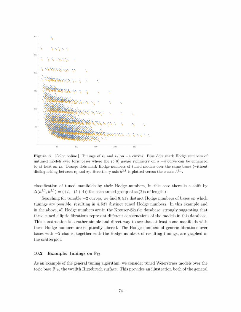
50 100 150 200 250

50

100

150

200

250

300

Figure 3. [Color online.] Tunings of e6 and e7 on −4 curves. Blue dots mark Hodge numbers ofuntuned models over toric bases where the so(8) gauge symmetry on a −4 curve can be enhancedto at least an e6. Orange dots mark Hodge numbers of tuned models over the same bases (withoutdistinguishing between e6 and e7. Here the y axis h2,1 is plotted versus the x axis h1,1.

classification of tuned manifolds by their Hodge numbers, in this case there is a shift by∆(h1,1, h2,1) = (+l,−(l + 4)) for each tuned group of su(2)s of length l.

Searching for tunable −2 curves, we find 8, 517 distinct Hodge numbers of bases on whichtunings are possible, resulting in 4, 537 distinct tuned Hodge numbers. In this example andin the above, all Hodge numbers are in the Kreuzer-Skarke database, strongly suggesting thatthese tuned elliptic fibrations represent different constructions of the models in this database.This construction is a rather simple and direct way to see that at least some manifolds withthese Hodge numbers are elliptically fibered. The Hodge numbers of generic fibrations overbases with −2 chains, together with the Hodge numbers of resulting tunings, are graphed inthe scatterplot.

10.2 Example: tunings on F12

As an example of the general tuning algorithm, we consider tuned Weierstrass models over thetoric base F12, the twelfth Hirzebruch surface. This provides an illustration both of the general

– 74 –

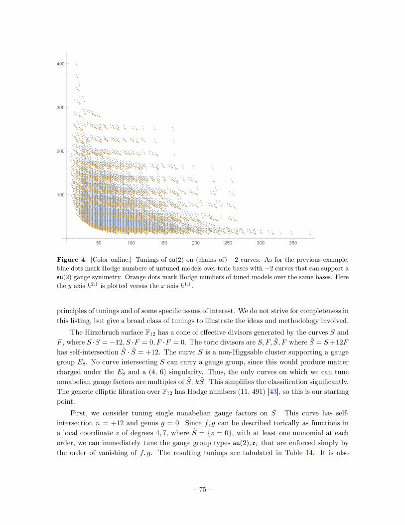
50 100 150 200 250 300 350

100

200

300

400

Figure 4. [Color online.] Tunings of su(2) on (chains of) −2 curves. As for the previous example,blue dots mark Hodge numbers of untuned models over toric bases with −2 curves that can support asu(2) gauge symmetry. Orange dots mark Hodge numbers of tuned models over the same bases. Herethe y axis h2,1 is plotted versus the x axis h1,1.

principles of tunings and of some specific issues of interest. We do not strive for completeness inthis listing, but give a broad class of tunings to illustrate the ideas and methodology involved.

The Hirzebruch surface F12 has a cone of effective divisors generated by the curves S andF , where S ·S = −12, S ·F = 0, F ·F = 0. The toric divisors are S, F, S, F where S = S+12F

has self-intersection S · S = +12. The curve S is a non-Higgsable cluster supporting a gaugegroup E8. No curve intersecting S can carry a gauge group, since this would produce mattercharged under the E8 and a (4, 6) singularity. Thus, the only curves on which we can tunenonabelian gauge factors are multiples of S, kS. This simplifies the classification significantly.The generic elliptic fibration over F12 has Hodge numbers (11, 491) [43], so this is our startingpoint.

First, we consider tuning single nonabelian gauge factors on S. This curve has self-intersection n = +12 and genus g = 0. Since f, g can be described torically as functions ina local coordinate z of degrees 4, 7, where S = {z = 0}, with at least one monomial at eachorder, we can immediately tune the gauge group types su(2), e7 that are enforced simply bythe order of vanishing of f, g. The resulting tunings are tabulated in Table 14. It is also

– 75 –

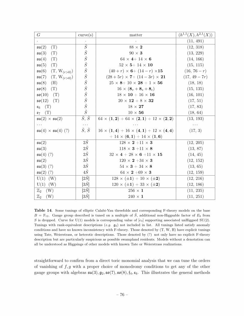
G curve(s) matter (h1,1(X), h2,1(X))

· · · (11, 491)su(2) (T) S 88 × 2 (12, 318)su(3) (T) S 90 × 3 (13, 229)su(4) (T) S 64 × 4+ 14 × 6 (14, 166)su(5) (T) S 52 × 5+ 14 × 10 (15, 115)su(6) (T, W(r>0)) S (40 + r) × 6+ (14− r) ×15 (16, 76− r)su(7) (T, W(r>0)) S (28 + 5r) × 7+ (14− 3r) × 21 (17, 49− 7r)su(8) (H) S 25 × 8+ 10 × 28 + 1 × 56 (18, 18)so(8) (T) S 16 × (8v + 8s + 8c) (15, 135)so(10) (T) S 18 × 10 + 16 × 16 (16, 101)so(12) (T) S 20 × 12 + 8 × 32 (17, 51)e6 (T) S 18 × 27 (17, 83)e7 (T) S 10 × 56 (18, 64)su(2) × su(2) S, S 64 × (1,2) + 64 × (2,1) + 12 × (2,2) (13, 193)· · · · · · · · · · · ·su(4) × su(4) (?) S, S 16 × (1,4) + 16 × (4,1) + 12 × (4,4) (17, 3)

+ 14 × (6,1) + 14 × (1,6)

su(2) 2S 128 × 2 +11 × 3 (12, 205)su(3) 2S 118 × 3 +11 × 8 (13, 87)su(4) (?) 2S 32 × 4 + 28 × 6 +11 × 15 (14, 45)su(2) 3S 120 × 2 +34 × 3 (12, 152)su(3) (?) 3S 54 × 3 + 34 × 8 (13, 65)su(2) (?) 4S 64 × 2 +69 × 3 (12, 159)U(1) (W) [2S] 128 × (±1) + 10 × (±2) (12, 216)U(1) (W) [3S] 120 × (±1) + 33 × (±2) (12, 186)Z2 (W) [2S] 256 × 1 (11, 235)Z2 (W) [3S] 240 × 1 (11, 251)

Table 14. Some tunings of elliptic Calabi-Yau threefolds and corresponding F-theory models on the baseB = F12. Gauge group described is tuned on a multiple of S, additional non-Higgsable factor of E8 fromS is dropped. Curve for U(1) models is corresponding value of [e3] supporting associated unHiggsed SU(2).Tunings with rank-equivalent descriptions (e.g. g2) not included in list. All tunings listed satisfy anomalyconditions and have no known inconsistency with F-theory. Those denoted by (T, W, H) have explicit tuningsusing Tate, Weierstrass, or heterotic descriptions. Those denoted by (?) not only have no explicit F-theorydescription but are particularly suspicious as possible swampland residents. Models without a denotation canall be understood as Higgsings of other models with known Tate or Weierstrass realizations.

straightforward to confirm from a direct toric monomial analysis that we can tune the ordersof vanishing of f, g with a proper choice of monodromy conditions to get any of the othergauge groups with algebras su(3), g2, so(7), so(8), f4, e6. This illustrates the general methods

– 76 –

of §4.3 in a specific context.The classical groups with algebras su(N), sp(N), so(N) must be considered separately.

We focus attention particularly on the SU(N) groups. For su(N), N = 6, 7 there are exoticmatter contents that can be tuned using Weierstrass as described in §7 [35]; these are includedin the Table. For SU(N) and Sp(k), from the matter spectrum in Table 4 it is clear that atN = 2k = 10 there is a problem as the number of fundamental representations becomesnegative. In fact, a Tate analysis indicates that tuning su(8) eliminates the single monomialof a6 that has order ≤ 5 on the −12 curve, forcing a non-minimal singularity there. This isan example of the constraint discussed in §6.4 that a 0-curve with an e8 on one side cannothave an su(N) with N ≥ 8 on the other side tuned using Tate. This is an example of a tuningin the swampland, which looks consistent from the low-energy point of view but may not beallowed in F-theory. Note that the groups that we can tune in this way are subgroups of E8,matching with the expectation that any tuning on this base should have a heterotic dual,with the resulting gauge group realized from an E8 bundle over K3 with instanton number24. An explicit construction was given in [35] for non-Tate Weierstrass tunings of su(8) withr matter fields in the triple-antisymmetric (56) representation; there it was argued that theonly heterotic dual to a tuning on the +12 curve of F12 has r = 1. The other Weierstrasstunings thus must have singularities15 when restricted to the compact base F12. From thelow-energy point of view it seems quite obscure why an E8× SU(8) theory constructed in thisway would be inconsistent with r = 0 but consistent with r = 1. Understanding this kind ofquestion better and in more generality is an interesting area for further research.

Since S is a non-rigid divisor (n ≥ 0), we can tune multiple independent gauge factors ondifferent curves Σi in this divisor class, which will then intersect one another with Σi · Σj =

12. For example, tuning two SU(2) factors on such curves gives a model with gauge group(E8×) SU(2) × SU(2), where there are 12 bifundamental fields in the (2,2) representation.From the spectrum and anomaly constraints we would expect to be able to tune variousproduct groups. It is fairly straightforward to see using Tate and the toric picture that itshould be possible to tune any product of groups SU(N1) × · · ·× SU(Nk) with

∑iNi < 8,

though we do not pursue the details here. Cases with∑

iNi = 8 are less clear and would beinteresting to explore in more detail. Note that these product group configurations can beunderstood from Higgsing on k-index antisymmetric representations of the su(N) models on S(see, e.g., [35] for an explicit discussion of several examples of such Higgsing in Weierstrass anddual heterotic descriptions). For example, Higgsing su(6) on a two-index antisymmetric (15)representation gives a model with gauge algebra su(2)⊕su(4), while Higgsing on a three-indexantisymmetric (20) gives a model with gauge algebra su(3)⊕ su(4). The su(4)⊕ su(4) modelthat is allowed by anomalies would in principle come from an anomaly-allowed model with ansu(8) gauge algebra and a 4-index antisymmetric matter field, but constructing a Weierstrassmodel for such configurations seems problematic [35]. Any model that can be realized in fieldtheory from the Higgsing of a model with a good F-theory description must also have a good

15Thanks to N. Raghuram for confirming this in the case r = 0.

– 77 –

F-theory description, even if the explicit Weierstrass construction is difficult to identify. Thus,the product groups with

∑iNi < 8 are also naturally understood as Higgsings of the models

with a single su(N) algebra on S.

Now let us consider tunings on the curve Σ = 2S. This curve has self-intersection n = 48,and from −K · Σ = 2(−K · Σ) = 28, we have g = 11. From Table 7, we see that anomaliessuggest that we can tune such models for SU(2), SU(3), and SU(4). Roughly, we are tuningon a curve described by a quadratic in the coordinate z that vanishes on S, so as for su(8) on S,the su(4) algebra on 2S may be problematic. The su(2) and su(3) models can be understoodin field theory from the Higgsing of the su(2)⊕su(2) and su(3)⊕su(3) models described aboveon a bifundamental field [35], and thus must exist in F-theory. The su(4) model on 2S is alsounclear from this point of view.

Similarly, we can consider tuning SU(2) and SU(3) models on 3S (n = 108, g = 34) andSU(2) on 4S (n = 192, g = 69). We have not attempted to explicitly construct Weierstrassmodels for these theories; the first of these should arise from Higgsing of an su(2)⊕su(2)⊕su(2)

model on S + S + S, which should in turn come from a Higgsing of su(6) on S, while theothers are likely problematic though acceptable from anomaly cancellation.

From these realizations of SU(2) and other nonabelian groups on higher genus curves wecan also proceed to implement the construction of U(1) models as discussed in §8. As discussedin the main body of the text, U(1) models and their spectra can be realized from Higgsings ofnonabelian models over the same base (which can be allowed to have some singularities thatare removed in the Higgsing). In the simplest cases, we achieve the U(1) model by Higgsingan SU(2) with generic matter; these can be explicitly realized using the Morrison-Park form[71]. In this case, we can consider the SU(2) realizations on kS for k = 2, 3. These give U(1)theories with various spectra, as listed in the table. Many further U(1) models with explicitWeierstrass models could be constructed with q = 3 charges through matter transitions in theunHiggsed SU(2) theory to SU(2) models with 4 matter, as discussed in [36]. and the supersetof all such models could be constructed by transferring an arbitrary number of groups of 3adjoints into 4’s, though Weierstrass models for all these are not known. Furthermore, manyU(1) × U(1) models with generic matter spectra could be constructed using the methods of[34], and the hypothetical superset of all U(1)k models may be constructable at the level ofspectra by considering all Higgsings of nonabelian models including those constructed above,though we have neither a method for explicitly constructing Weierstrass models in these cases,nor a proof that this exhausts all possibilities for k > 2. We do not explore these considerationsfurther here.

We conclude by constructing the model with discrete Z2 gauge group with what seemsto be the largest value of h2,1. This follows from taking the k = 2 generic U(1) model aboveand Higgsing on a field of charge 2, following [72]. Many more models with discrete gaugegroups and various charges could be constructed, some explicitly in Weierstrass, and a largersuperset by considering all Higgsings on non-unit charges of abelian U(1)k models.

– 78 –

11 Conclusions and Outlook

In this paper we have reported on progress towards a complete description of the set of Weier-strass tunings over a given complex surface B that supports elliptic Calabi-Yau threefolds.These Weierstrass tunings can be used to classify elliptic Calabi-Yau threefolds and to studyF-theory supergravity and SCFT models in six dimensions. In particular, for a given base Bthe results accumulated here give a set of constraints on the set of possible tunings over B,which give a finite superset of the finite set of consistent tunings. While we have not com-pletely solved the tuning classification problem, we have framed the structure of the problem,developed many of the components needed for a full solution, and identified a few remainingcomponents that need a more complete analysis for a full understanding.

The tools developed in this work can be used in a number of ways, including generatingexamples of elliptic Calabi-Yau threefolds and F-theory models with particular features ofinterest, the classification of elliptic Calabi-Yau threefolds and corresponding 6D supergravitytheories, and exploration of the “swampland” of 6D theories that seem consistent but cannotbe realized explicitly in F-theory. In this concluding section we summarize the specific resultsof this paper as well as a set of further issues to be addressed, and we discuss the implicationsfor the 6D swampland and the potential extension of this kind of analysis to 4D F-theorymodels.

11.1 Summary of results

This progress extends previous work in the following ways:

• We have completely classified local tunings of arbitrary gauge groups with generic matteron a single rational curve, and shown in all cases except su(N) that the tunings allowedby anomaly cancellation can be realized in explicit local Weierstrass/Tate models; forsu(N) we have found Tate models for almost all cases, with a few exceptions at largeodd N and divisors of positive self-intersection for which Tate models are impossibleand no Weierstrass models are known.

• We have completely classified local tunings in the same way over all multiple-curvenon-Higgsable clusters.

• We have classified allowed local tunings on a pair of intersecting rational curves, andshown that a large fraction of anomaly-allowed tunings can be realized by Tate or Weier-strass models, but we have also identified quite a few exceptions.

• We have identified some specific configurations, such as su(10) ⊕ su(3) and g2 ⊕ sp(4)

on a pair of intersecting curves of self-intersections −2 and −1, that are allowed byanomalies but cannot be realized through a Tate construction in F-theory. These rep-resent a component of the “swampland” both for supergravity theories and for SCFTs,and must be explained if the assertion of F-theory universality for 6D SCFT’s is to be

– 79 –

proven. We have found a substantially larger number of configurations in the supergrav-ity swampland that do not have low-energy field theory descriptions through an SCFTwith gravity decoupled as they involve curves of nonnegative self-intersection.

• We have identified extremal configurations of −2 curves, associated with degenerateelliptic curves satisfying Σ · Σ = −K · Σ = 0, as loci that in F-theory admit a finitenumber of su(N) tunings though low-energy consistency does not constrain N in anyknown way.

• We have investigated the validity of the “E8” rule [18], which constrains the gaugefactors that can be tuned on divisors that intersect a −1 curve carrying no gauge group,in the context of tuning enhanced gauge symmetries. We found that the E8 rule is anecessary condition for tunings to be possible, but may not be a sufficient condition assome combinations of gauge groups that live within E8 cannot be realized using Tate.We also identified an analogous rule for curves of self-intersection 0.

• Combining the preceding results gives a complete set of tools that can in principleproduce the finite set of all possible tunings over toric curves in toric bases. Work inthis direction is in progress [94]. In the toric case, each prospective tuning can be checkedfor global consistency in a global Weierstrass model using toric methods.

• These tools, in the context of 6D SCFT’s, give a systematic description of tuningsof an SCFT in terms of a Weierstrass or Tate model on the set of contracted curves,complementing the analysis of [19]. In particular, this work goes beyond that reported in[19] in that we systematically construct explicit Weierstrass models for the configurationsallowed by anomaly constraints, and identify some new configurations that do not admitTate tunings and do not have known or straightforward Weierstrass models, yet whichsatisfy low-energy consistency conditions. These tunings can also be applied in theclosely related context of F-theory realizations of little string theories [68].

• We have used anomaly cancellation to classify the set of possible tunings over curves ofarbitrary genus that are acceptable from low-energy considerations.

• We have computed explicitly the Hodge number shifts for the elliptic Calabi-Yau three-fold for all the preceding tunings.

• We have provided geometric proofs of strong constraints on local combinations of al-lowed tunings, matching constraints from anomaly considerations. In particular, wehave shown that the only possible pairs of gauge group factors that can arise on inter-secting divisors, and hence the only combinations of gauge groups that can share matterin any low-energy theory arising from F-theory, have one of the five combinations ofalgebras listed in Table 10 (or arise as a product subgroup of one of the allowed realizedindividual or product groups after an appropriate breaking).

– 80 –

• We have given a general procedure for classifying allowed tunings of non-generic matterand abelian gauge fields, which will give a finite set of tunings allowed over any givenbase, and which should be a superset of the complete set that can be explicitly realizedin F-theory.

11.2 The 6D N = 1 “tuning” swampland

In general, one of the goals of this work is to narrow down the “swampland” of models thatseem consistent from low-energy considerations but that lack UV descriptions in string/F-theory [23]. For 6D supergravity models, this problem can be broken into two parts: first,the matching of completely Higgsed 6D supergravity models to F-theory constructions, andsecond the matching of all possible gauge enhancements through tuning/unHiggsing in theF-theory and supergravity models. There are still substantial outstanding questions relatedto the first part; in particular, we do not have a proof that a low-energy model with a BPSdyonic string of Dirac self-charge -3 or below implies the presence of a non-Higgsable gaugefield, while F-theory implies this condition. In this paper we address the second part of thequestion: given a completely Higgsed 6D supergravity theory with an F-theory realizationwe ask whether all possible unHiggsings of the 6D SUGRA theory that are consistent withanomaly cancellation can be realized as tunings of the corresponding F-theory model. Bycomparing field theory and F-theory geometric analysis of various local combinations of gaugegroups over different curve types, we have shown that in almost all cases, F-theory reproducesprecisely the set of gauge groups and matter through tunings that are allowed by anomalycancellation conditions and other low-energy consistency constraints. We have also, however,identified some situations where field theory and F-theory are not in agreement, or seem fromour current understanding not to be in agreement. We list these here.

Tunings on a single divisor For local tunings of generic matter types over a single rationalcurve, we found that virtually everything that is allowed by anomaly cancellation has anexplicit Tate or Weierstrass realization. The only class of exceptions were the tunings of large-rank su(N) algebras listed in Table 6. For those cases, Tate models are not possible. In someexamples such as su(21) and su(23) on a +1 curve, a straightforward approach to Weierstrassmodels also fails; although we have not proven rigorously that a Weierstrass realization isimpossible this seems likely to be true as other known non-Tate Weierstrass models realizeexotic matter. These swampland examples may have a low-energy inconsistency, may berealizable through exotic Weierstrass models or may be stuck in the swampland. The largesu(N) tunings constitute the complete set of single-divisor swampland examples encounteredin this work.

Tunings on a pair of divisors For local tunings of generic matter over a pair of rationalcurves that intersect at a single point, we found a larger class of instances of models thatare allowed through anomalies but not through Tate constructions. In addition to a coupleof known examples such as so(8) ⊕ su(2) when the su(2) is on a −2 curves (which is knownto have field theory inconsistencies [60]), we found other examples of algebras su(N)⊕ sp(k),

– 81 –

su(N) ⊕ su(M), g2 ⊕ sp(k), and so(N) ⊕ sp(k) that are acceptable according to anomalycancellation but do not have Tate realizations. A simple example is su(2j + 1) ⊕ su(2j + 8)

on a pair of curves of self-intersection −1,−2. A further list of examples of tunings on twointersecting curves without Tate forms is given in §6.2. Like the examples on a single rationalcurve, we do not have a proof that Weierstrass models cannot be found for any of these cases,though we do not expect a non-Tate Weierstrass model in any of these cases with genericmatter content.

Tunings on degenerate elliptic curves As discussed in §5.2.2, §6.5, there are some localcombinations of divisors, for example a sequence of two or more −2 curves mutually inter-secting in a loop, which naively admit an infinite number of gauge group tunings with a finitenumber of moduli needed for the tuning. These correspond to low-energy 6D supergravitytheories with T ≥ 9 with no apparent inconsistency. We have identified these configurations inF-theory as degenerate elliptic curves satisfying Σ ·Σ = −K ·Σ = 0. From the F-theory pointof view su(N) gauge groups can be tuned on such curves with N taking values only up to aspecific bound associated with the constraint ∆ = −12K. As discussed in [9], however, thereis no low-energy understanding at this time of this “Kodaira constraint,” so that for effectivecones containing such −2 curve configurations there is effectively an infinite swampland. Thisis an example of the more general issue that adding a gauge group with only adjoint matter(essentially an N = (1, 1) multiplet) does not affect anomaly conditions, and can be limitedin F-theory but not in the low-energy theory.

Exotic matter We have listed in §7 some exotic matter content for which there are knownconstructions. Other types of matter appear to be allowed by the anomaly constraints, butare at this point lacking Weierstrass constructions. The resolution of this part of the tuningswampland will be addressed further elsewhere.

Constraints from divisors without gauge factorsConstraints such as the E8 rule that involve divisors that do not carry gauge factors

are not currently understood from 6D supergravity, though they can be partly explained inSCFT limits. We have identified some possible exceptions to the sufficiency of E8 rule fordetermining allowed tunings; for example, su(5)⊕ su(5) and su(9)⊕ · cannot be tuned usingthe Tate procedure on a pair of divisors that intersect a −1 curve without forcing a gaugefactor on the −1 curve. Such examples suggest some new low-energy consistency conditionin both supergravity and SCFT or a novel construction of non-Tate Weierstrass models withgeneric matter for certain groups. We have also sketched out the analogue of the E8 rule fordivisors of self-intersection 0. These kinds of constraints are somewhat similar to the constraintthat, for example, a low-energy theory containing a BPS dyonic string of Dirac self-charge−3, which would correspond in F-theory to a −3 curve in the base, needs to carry a gaugegroup su(3) in this case. A related set of issues is the distinction between type III, IV , andI2, I3 realizations of su(2), su(3), which have slightly different rules for intersections but arenot easily distinguished in the low-energy theory. Understanding the E8 rule and these other

– 82 –

related conditions from low-energy considerations is an important part of the outstandingproblem of clearing the 6D swampland.

Abelian gauge factors We have outlined an algorithm, following [34], which in principlegives a superset of the set of possible F-theory models with abelian gauge field content. Thisalgorithm is based on Higgsing of nonabelian gauge factors with adjoint matter. Provingthat all abelian F-theory models can be constructed in this fashion, and matching preciselywith low-energy anomaly constraints, particularly for higher-rank abelian groups, remains anoutstanding research problem.

11.3 Tate vs. Weierstrass

One interesting question that arises in attempting to do generic tunings is the extent to whichTate models can produce the full set of possible tunings. It is known that there are Weierstrasstunings of su(N) with N = 6, 7, 8 that cannot be realized through Tate [32, 33, 35], thoughthese are associated with exotic matter (e.g., in the three-index antisymmetric representation).We have also identified cases of so(N) with N = 13 on curves of self-intersection n with n

even but not n = −4, where Weierstrass models can be realized but Tate cannot. It is knownthat Weierstrass and Tate tunings of su(N) are equivalent for N < 6, and are believed to bemore generally equivalent when exotic matter representations are not included. It thereforeseems possible that many of the tunings found here on a single curve or a pair of curves thatdo not have Tate realizations also do not have Weierstrass realizations with generic mattercontent and represent elements of the swampland. 16 But identifying precisely the set of caseswhere Tate and Weierstrass forms are not equally valid, is a remaining task that needs to becompleted to clear out this part of the F-theory swamp.

11.4 4D F-theory models

The focus of this paper has been on 6D supergravity theories described by F-theory compact-ifications on complex surfaces. An analogous set of constructions give 4D N = 1 supergravitytheories from F-theory compactifications on complex threefolds. While the 4D case is muchless well understood, and the connection between the underlying F-theory geometry and low-energy physics is made more complicated by fluxes, D-brane world-volume degrees of freedom,a nontrivial superpotential, and a weaker set of anomaly constraints, the basic principles oftuning that we have developed here are essentially the same in 4D. For threefold bases, di-visors that have a local toric description can again be analyzed torically, and we can writeWeierstrass and Tate models for the kinds of gauge groups and matter that can be tuned.

Perhaps the clearest result of this paper that immediately generalizes to 4D F-theoryconstructions is the constraint derived in §6.1 that limits the possible products of gaugegroups on intersecting divisors to only the five (families of) algebra pairings listed in Table 10.

16(Added in v2:) David Morrison has pointed out that some models with groups that cannot be realizedusing Tate can have Weierstrass realizations when there is a discrete Mordell-Weil group associated with aquotient of the usual simply-connected simple group associated with a given algebra.

– 83 –

This constraint is also valid for tunings in 4D F-theory models, with the same microscopicderivation from the Weierstrass analysis. A consequence of this result is that we have shownin general that any N = 1 low-energy theory of supergravity coming from F-theory can onlyhave matter charged under multiple gauge factors when the factors are either among those inTable 10, or both factors come from the breaking of a larger single group (or product group)such as e8 that is realized in F-theory.

More generally, the methods summarized in §2.2 in association with (2.11), which weredeveloped in [95, 38], can be used to identify the non-Higgsable gauge group and local tuningson any local combination of divisors an a base threefold, with explicit Weierstrass and Tateconstructions for local toric geometries. For single divisors, the set of possible tunings willfollow a similar pattern to that found here in §4. The non-Higgsable clusters over single toricdivisors were analyzed (in the context of P1 bundles) in [95, 96], and the finite set of possibletunings over such combinations of divisors can be constructed using the same methods asthose used here and is again finite in most cases. A similar analysis is also possible for divisorswith a positive or less negative normal bundle. For example, in analogy with a +1 curve, itis straightforward to confirm that any of the exceptional gauge algebras can be tuned on adivisor with the geometry of D = P2 with a normal bundle of +H, and that a Tate form forSp(k) and SU(2k) can be realized in a toric model, for k ≤ 16, in analogy with the bound of12 for the same tunings on the +1 curve [33].

Also for multiple intersecting divisors, a similar analysis can be carried out.The difficult part of generalizing the analysis of this paper to 4D is the absence of strong

low-energy constraints for 4D N = 1 supergravity models. While in 6D, as we have shownhere, the set of constraints imposed by low-energy anomaly cancellation conditions is almostprecisely equivalent to the constraints imposed by Weierstrass tuning, in 4D the known low-energy constraints are much weaker, so the apparent swampland is much larger. Whether thisis an indication that F-theory describes a much smaller part of the space of consistent 4Dsupergravity theories, or we are simply lacking insight into 4D low-energy consistency condi-tions, is an important open question for further research (see [97] for some initial investigationsin this direction).

11.5 Outstanding questions

In this paper we have made progress towards a complete classification of allowed tuningsfor Weierstrass models over a given base. A desirable final goal of this program would be acomplete set of local constraints (in terms only of gauge algebras, matter representations, andthe self-intersection matrix of the base) such that a fibration exists that produces a Weierstrassmodel for a Calabi-Yau threefold and corresponding 6D supergravity model if and only if thatfibration satisfies all of the local constraints. Here we summarize some questions that stillneed to be addressed to complete the classification and to match Weierstrass tunings in 6DF-theory models to low-energy supergravity theories.

• The remaining local configurations in the “tuning swampland” summarized in §11.2

– 84 –

should hopefully be able to be identified either as allowed by as-yet-unknown Weierstrasstunings, or as inconsistent in UV-complete quantum 6D supergravity theories.

• We have addressed in this paper local constraints associated with the tunings of gaugegroups and matter over a single divisor corresponding to a curve in the base and theset of other curves intersecting that divisor. We do not know that every model thatsatisfies all local constraints of this type is globally consistent, though we do not knowof any counterexamples. It would be desirable to either prove that local constraints aresufficient or identify conflicts that can arise nonlocally.

• We have only checked Weierstrass/Tate realizations for rational curves with local toricdescriptions. It would be desirable to expand the methodology to higher-genus curveswithout a local toric description.

• Tuned gauge factors such as g2 that can be broken without decreasing rank give ad-ditional contributions to h2,1(X) from the associated charged matter fields that areuncharged under the smaller group. This should be understood better geometrically,and may also be related to the issue of tuning su(N) factors on degenerate ellipticcurves; in both cases the essential issue is the addition of a (1, 1) multiplet with gaugebosons and hypermultiplets that precisely cancel anomaly constraints. The connectionbetween this phenomenon and the topology of the elliptic Calabi-Yau threefold shouldbe better understood, and will be described further elsewhere [45].

• The classification of exotic matter representations, particularly those realized by gaugegroups supported on singular divisors in the base, must be completed. In particular, themethod of analysis in §7 assumed that any exotic matter configuration can be realizedas a tuning of a generic matter configuration — that is, that there are no non-Higgsableexotic matter configurations possible. While we believe that this is true we do not havea rigorous proof of this statement.

• It needs to be shown whether the approach used here of constructing abelian gaugefactors from Higgsing of nonabelian tuned gauge factors is able to produce all abeliangauge structures of arbitrary rank; even if this is possible, a systematic understandingof how this can be implemented for higher-rank gauge groups and what singularities arepossible in the nonabelian enhanced model for a consistent Higgsed abelian theory mustbe better understood.

A further set of questions, which fit into this general framework but which go beyond thegoal of classifying all tunings over a given base surface, include the following:

• We have not addressed the question of different resolutions of the Kodaira singularities,which are not relevant for the low-energy 6D physics, but would need to be addressed ingeneral for a complete classification of smooth elliptic Calabi-Yau threefolds, as discussedin §2.5.

– 85 –

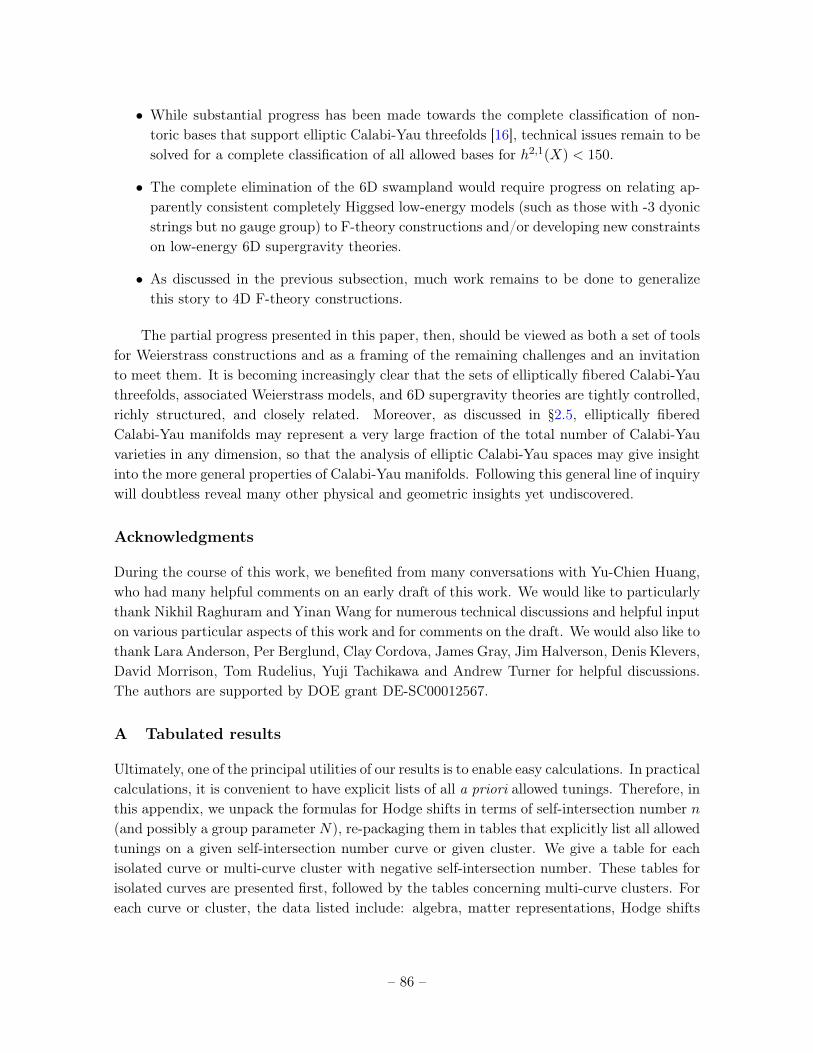
• While substantial progress has been made towards the complete classification of non-toric bases that support elliptic Calabi-Yau threefolds [16], technical issues remain to besolved for a complete classification of all allowed bases for h2,1(X) < 150.

• The complete elimination of the 6D swampland would require progress on relating ap-parently consistent completely Higgsed low-energy models (such as those with -3 dyonicstrings but no gauge group) to F-theory constructions and/or developing new constraintson low-energy 6D supergravity theories.

• As discussed in the previous subsection, much work remains to be done to generalizethis story to 4D F-theory constructions.

The partial progress presented in this paper, then, should be viewed as both a set of toolsfor Weierstrass constructions and as a framing of the remaining challenges and an invitationto meet them. It is becoming increasingly clear that the sets of elliptically fibered Calabi-Yauthreefolds, associated Weierstrass models, and 6D supergravity theories are tightly controlled,richly structured, and closely related. Moreover, as discussed in §2.5, elliptically fiberedCalabi-Yau manifolds may represent a very large fraction of the total number of Calabi-Yauvarieties in any dimension, so that the analysis of elliptic Calabi-Yau spaces may give insightinto the more general properties of Calabi-Yau manifolds. Following this general line of inquirywill doubtless reveal many other physical and geometric insights yet undiscovered.

Acknowledgments

During the course of this work, we benefited from many conversations with Yu-Chien Huang,who had many helpful comments on an early draft of this work. We would like to particularlythank Nikhil Raghuram and Yinan Wang for numerous technical discussions and helpful inputon various particular aspects of this work and for comments on the draft. We would also like tothank Lara Anderson, Per Berglund, Clay Cordova, James Gray, Jim Halverson, Denis Klevers,David Morrison, Tom Rudelius, Yuji Tachikawa and Andrew Turner for helpful discussions.The authors are supported by DOE grant DE-SC00012567.

A Tabulated results

Ultimately, one of the principal utilities of our results is to enable easy calculations. In practicalcalculations, it is convenient to have explicit lists of all a priori allowed tunings. Therefore, inthis appendix, we unpack the formulas for Hodge shifts in terms of self-intersection number n(and possibly a group parameter N), re-packaging them in tables that explicitly list all allowedtunings on a given self-intersection number curve or given cluster. We give a table for eachisolated curve or multi-curve cluster with negative self-intersection number. These tables forisolated curves are presented first, followed by the tables concerning multi-curve clusters. Foreach curve or cluster, the data listed include: algebra, matter representations, Hodge shifts

– 86 –

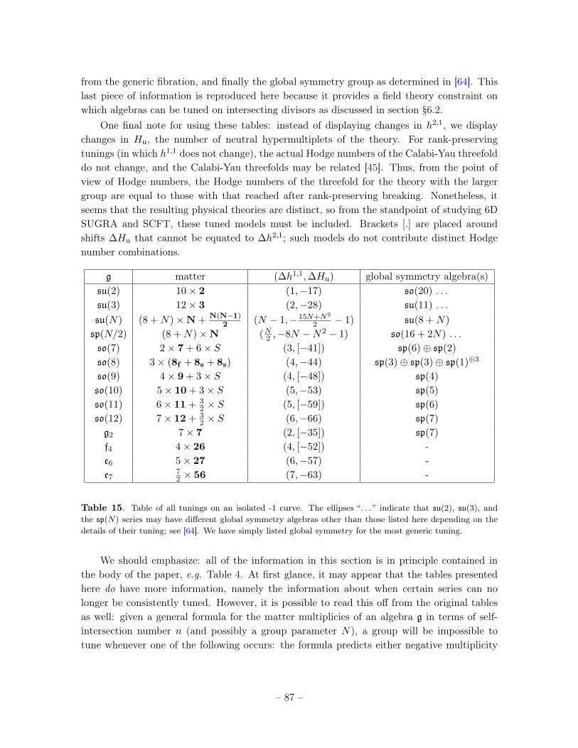
from the generic fibration, and finally the global symmetry group as determined in [64]. Thislast piece of information is reproduced here because it provides a field theory constraint onwhich algebras can be tuned on intersecting divisors as discussed in section §6.2.

One final note for using these tables: instead of displaying changes in h2,1, we displaychanges in Hu, the number of neutral hypermultiplets of the theory. For rank-preservingtunings (in which h1,1 does not change), the actual Hodge numbers of the Calabi-Yau threefolddo not change, and the Calabi-Yau threefolds may be related [45]. Thus, from the point ofview of Hodge numbers, the Hodge numbers of the threefold for the theory with the largergroup are equal to those with that reached after rank-preserving breaking. Nonetheless, itseems that the resulting physical theories are distinct, so from the standpoint of studying 6DSUGRA and SCFT, these tuned models must be included. Brackets [.] are placed aroundshifts ∆Hu that cannot be equated to ∆h2,1; such models do not contribute distinct Hodgenumber combinations.

g matter (∆h1,1,∆Hu) global symmetry algebra(s)su(2) 10× 2 (1,−17) so(20) . . .su(3) 12× 3 (2,−28) su(11) . . .su(N) (8 +N)×N + N(N−1)

2 (N − 1,−15N+N2

2 − 1) su(8 +N)

sp(N/2) (8 +N)×N (N2 ,−8N −N2 − 1) so(16 + 2N) . . .so(7) 2× 7 + 6× S (3, [−41]) sp(6)⊕ sp(2)

so(8) 3× (8f + 8s + 8s) (4,−44) sp(3)⊕ sp(3)⊕ sp(1)⊕3

so(9) 4× 9 + 3× S (4, [−48]) sp(4)

so(10) 5× 10 + 3× S (5,−53) sp(5)

so(11) 6× 11 + 32 × S (5, [−59]) sp(6)

so(12) 7× 12 + 32 × S (6,−66) sp(7)

g2 7× 7 (2, [−35]) sp(7)

f4 4× 26 (4, [−52]) -e6 5× 27 (6,−57) -e7

72 × 56 (7,−63) -

Table 15. Table of all tunings on an isolated -1 curve. The ellipses “. . . ” indicate that su(2), su(3), andthe sp(N) series may have different global symmetry algebras other than those listed here depending on thedetails of their tuning; see [64]. We have simply listed global symmetry for the most generic tuning.

We should emphasize: all of the information in this section is in principle contained inthe body of the paper, e.g. Table 4. At first glance, it may appear that the tables presentedhere do have more information, namely the information about when certain series can nolonger be consistently tuned. However, it is possible to read this off from the original tablesas well: given a general formula for the matter multiplicies of an algebra g in terms of self-intersection number n (and possibly a group parameter N), a group will be impossible totune whenever one of the following occurs: the formula predicts either negative multiplicity

– 87 –

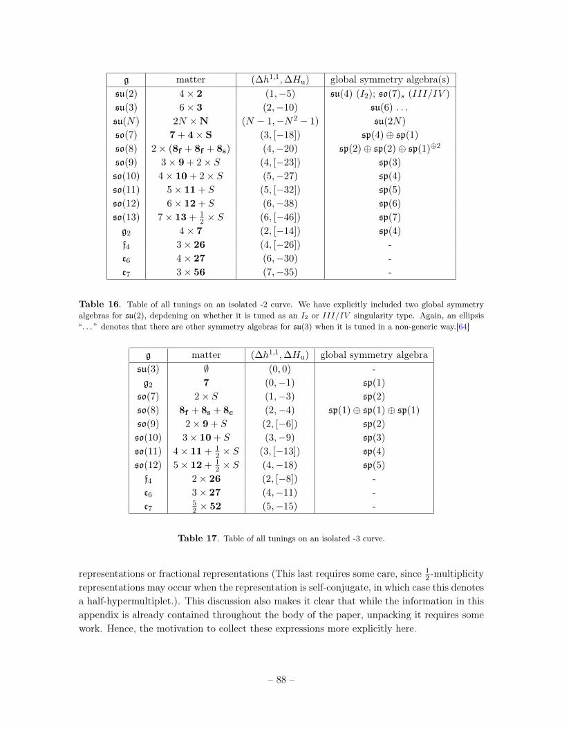
g matter (∆h1,1,∆Hu) global symmetry algebra(s)su(2) 4× 2 (1,−5) su(4) (I2); so(7)s (III/IV )su(3) 6× 3 (2,−10) su(6) . . .su(N) 2N ×N (N − 1,−N2 − 1) su(2N)

so(7) 7 + 4× S (3, [−18]) sp(4)⊕ sp(1)

so(8) 2× (8f + 8f + 8s) (4,−20) sp(2)⊕ sp(2)⊕ sp(1)⊕2

so(9) 3× 9 + 2× S (4, [−23]) sp(3)

so(10) 4× 10 + 2× S (5,−27) sp(4)

so(11) 5× 11 + S (5, [−32]) sp(5)

so(12) 6× 12 + S (6,−38) sp(6)

so(13) 7× 13 + 12 × S (6, [−46]) sp(7)

g2 4× 7 (2, [−14]) sp(4)

f4 3× 26 (4, [−26]) -e6 4× 27 (6,−30) -e7 3× 56 (7,−35) -

Table 16. Table of all tunings on an isolated -2 curve. We have explicitly included two global symmetryalgebras for su(2), depdening on whether it is tuned as an I2 or III/IV singularity type. Again, an ellipsis“. . . ” denotes that there are other symmetry algebras for su(3) when it is tuned in a non-generic way.[64]

g matter (∆h1,1,∆Hu) global symmetry algebrasu(3) ∅ (0, 0) -g2 7 (0,−1) sp(1)

so(7) 2× S (1,−3) sp(2)

so(8) 8f + 8s + 8c (2,−4) sp(1)⊕ sp(1)⊕ sp(1)

so(9) 2× 9 + S (2, [−6]) sp(2)

so(10) 3× 10 + S (3,−9) sp(3)

so(11) 4× 11 + 12 × S (3, [−13]) sp(4)

so(12) 5× 12 + 12 × S (4,−18) sp(5)

f4 2× 26 (2, [−8]) -e6 3× 27 (4,−11) -e7

52 × 52 (5,−15) -

Table 17. Table of all tunings on an isolated -3 curve.

representations or fractional representations (This last requires some care, since 12 -multiplicity

representations may occur when the representation is self-conjugate, in which case this denotesa half-hypermultiplet.). This discussion also makes it clear that while the information in thisappendix is already contained throughout the body of the paper, unpacking it requires somework. Hence, the motivation to collect these expressions more explicitly here.

– 88 –

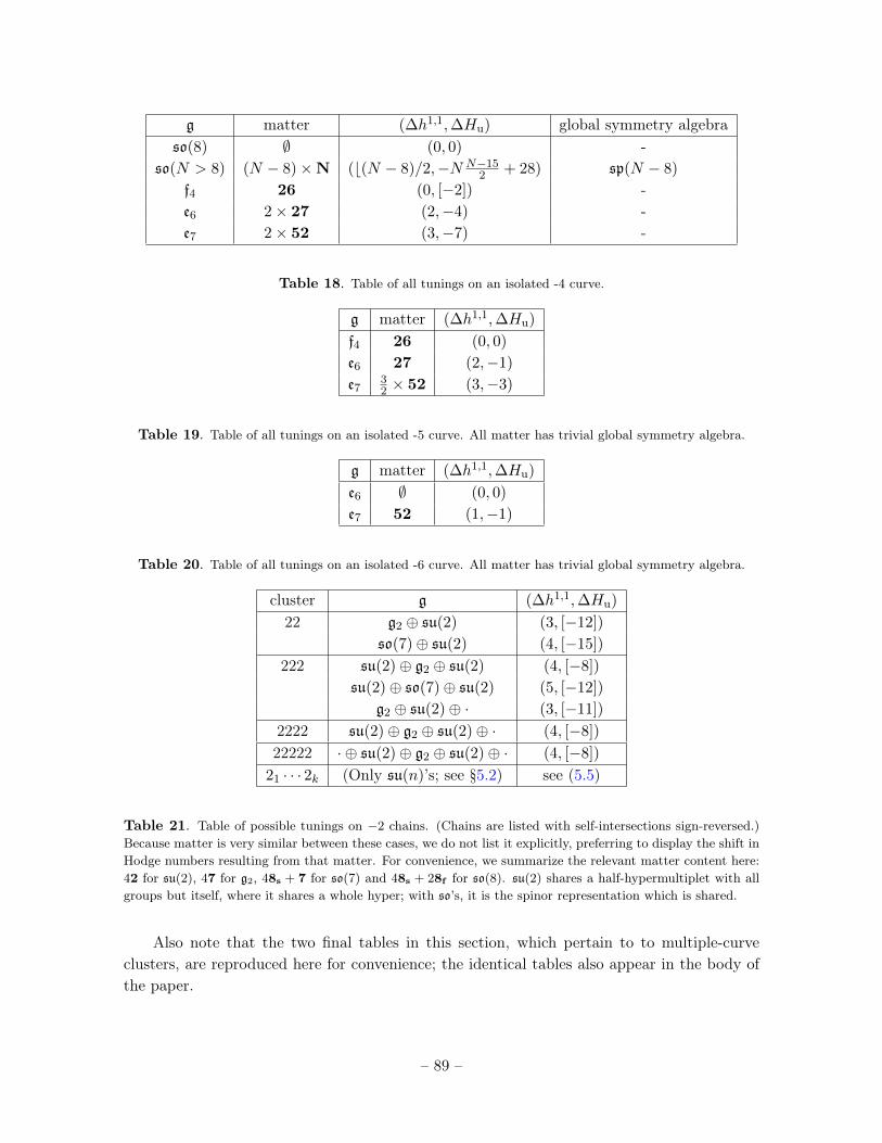
g matter (∆h1,1,∆Hu) global symmetry algebraso(8) ∅ (0, 0) -

so(N > 8) (N − 8)×N (b(N − 8)/2,−N N−152 + 28) sp(N − 8)

f4 26 (0, [−2]) -e6 2× 27 (2,−4) -e7 2× 52 (3,−7) -

Table 18. Table of all tunings on an isolated -4 curve.

g matter (∆h1,1,∆Hu)

f4 26 (0, 0)

e6 27 (2,−1)

e732 × 52 (3,−3)

Table 19. Table of all tunings on an isolated -5 curve. All matter has trivial global symmetry algebra.

g matter (∆h1,1,∆Hu)

e6 ∅ (0, 0)

e7 52 (1,−1)

Table 20. Table of all tunings on an isolated -6 curve. All matter has trivial global symmetry algebra.

cluster g (∆h1,1,∆Hu)

22 g2 ⊕ su(2) (3, [−12])

so(7)⊕ su(2) (4, [−15])

222 su(2)⊕ g2 ⊕ su(2) (4, [−8])

su(2)⊕ so(7)⊕ su(2) (5, [−12])

g2 ⊕ su(2)⊕ · (3, [−11])

2222 su(2)⊕ g2 ⊕ su(2)⊕ · (4, [−8])

22222 · ⊕ su(2)⊕ g2 ⊕ su(2)⊕ · (4, [−8])

21 · · · 2k (Only su(n)’s; see §5.2) see (5.5)

Table 21. Table of possible tunings on −2 chains. (Chains are listed with self-intersections sign-reversed.)Because matter is very similar between these cases, we do not list it explicitly, preferring to display the shift inHodge numbers resulting from that matter. For convenience, we summarize the relevant matter content here:42 for su(2), 47 for g2, 48s + 7 for so(7) and 48s + 28f for so(8). su(2) shares a half-hypermultiplet with allgroups but itself, where it shares a whole hyper; with so’s, it is the spinor representation which is shared.

Also note that the two final tables in this section, which pertain to to multiple-curveclusters, are reproduced here for convenience; the identical tables also appear in the body ofthe paper.

– 89 –

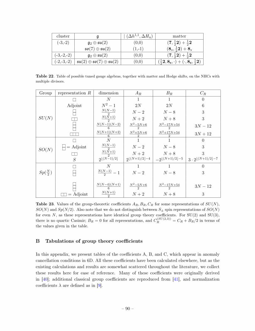
cluster g | (∆h1,1,∆Hu) matter(-3,-2) g2 ⊕ su(2) (0,0) (7, 1

22) + 122

so(7)⊕ su(2) (1,-1) (8s,122) + 8s

(-3,-2,-2) g2 ⊕ su(2) (0,0) (7, 122) + 1

22

(-2,-3,-2) su(2)⊕ so(7)⊕ su(2) (0,0) (122,8s, ·) + (·,8s, 1

22)

Table 22. Table of possible tuned gauge algebras, together with matter and Hodge shifts, on the NHCs withmultiple divisors.

Group representation R dimension AR BR CR

SU(N)

N 1 1 0Adjoint N2 − 1 2N 2N 6

N(N−1)2 N − 2 N − 8 3

N(N+1)2 N + 2 N + 8 3

N(N−1)(N−2)6

N2−5N+62

N2−17N+542 3N − 12

N(N+1)(N+2)6

N2+5N+62

N2+17N+542 3N + 12

SO(N)

N 1 1 0= Adjoint N(N−1)

2 N − 2 N − 8 3N(N+1)

2 N + 2 N + 8 3S 2b(N−1)/2c 2b(N+1)/2c−4 −2b(N+1)/2c−5 3 · 2b(N+1)/2c−7

Sp(N2 )

N 1 1 0N(N−1)

2 − 1 N − 2 N − 8 3

N(N−4)(N+1)6

N2−5N+62

N2−17N+542 3N − 12

= Adjoint N(N+1)2 N + 2 N + 8 3

Table 23. Values of the group-theoretic coefficients AR, BR, CR for some representations of SU(N),SO(N) and Sp(N/2). Also note that we do not distinguish between S± spin representations of SO(N)

for even N , as these representations have identical group theory coefficients. For SU(2) and SU(3),there is no quartic Casimir; BR = 0 for all representations, and C(SU(2,3))

R = CR + BR/2 in terms ofthe values given in the table.

B Tabulations of group theory coefficients

In this appendix, we present tables of the coefficients A, B, and C, which appear in anomalycancellation conditions in 6D. All these coefficients have been calculated elsewhere, but as theexisting calculations and results are somewhat scattered throughout the literature, we collectthese results here for ease of reference. Many of these coefficients were originally derivedin [40]; additional classical group coefficients are reproduced from [41], and normalizationcoefficients λ are defined as in [9].

– 90 –

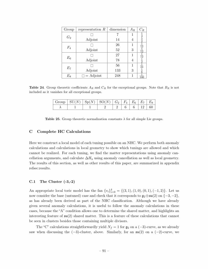
Group representation R dimension AR CR

G27 1 1

4

Adjoint 14 4 52

F426 1 1

12

Adjoint 52 3 512

E627 1 1

12

Adjoint 78 4 12

E756 1 1

24

Adjoint 133 3 16

E8 = Adjoint 248 1 1100

Table 24. Group theoretic coefficients AR and CR for the exceptional groups. Note that BR is notincluded as it vanishes for all exceptional groups.

Group SU(N) Sp(N) SO(N) G2 F4 E6 E7 E8

λ 1 1 2 2 6 6 12 60

Table 25. Group theoretic normalization constants λ for all simple Lie groups.

C Complete HC Calculations

Here we construct a local model of each tuning possible on an NHC. We perform both anomalycalculations and calculations in local geometry to show which tunings are allowed and whichcannot be realized. For each tuning, we find the matter representations using anomaly can-cellation arguments, and calculate ∆Hu using anomaly cancellation as well as local geometry.The results of this section, as well as other results of this paper, are summarized in appendixrefsec:results.

C.1 The Cluster (-3,-2)

An appropriate local toric model has the fan {vi}4i=0 = {(3, 1), (1, 0), (0, 1), (−1, 2)}. Let usnow consider the base (untuned) case and check that it corresponds to g2⊕su(2) on {−3,−2},as has already been derived as part of the NHC classification. Although we have alreadygiven several anomaly calculations, it is useful to follow the anomaly calculations in thesecases, because the “A” condition allows one to determine the shared matter, and highlights aninteresting feature of su(2) shared matter. This is a feature of these calculations that cannotbe seen in clusters besides those containing multiple divisors.

The “C” calculations straightforwardly yield Nf = 1 for g2 on a (−3)-curve, as we alreadysaw when discussing the (−3)-cluster, above. Similarly, for an su(2) on a (−2)-curve, we

– 91 –

obtain

Σ · Σ =λ2

3

(∑R

CR − CAdj

)

−2 =1

3

(N

2− 8

)N = 4 (C.1)

fundamentals. The “A” condition of bifundamental matter is more interesting in this case,because it dictates

ξi · ξj = λiλj∑R

AiRAjRx

ijR (C.2)

Recall,we are considering ξi · ξj = 1 for neighbors and is zero otherwise. The sum on the righthand side is over all shared representations between the two gauge groups, which (consistentwith the string theory description) can occur only between divisors that intersect. The Ai areall integer-valued (and must be positive), the xij denote the multiplicities of the representa-tions, and the λ are group theory coefficients introduced earlier. The key fact in this case isthat, whereas λ = 1 for su(2), λ = 2 for g2, so(7), and so(8) (λ is always the same for differnetgauge algrebras distinguished only by monodromy). Since A = 1 by definition for fundamentalrepresentations, the equation now reads 1 = 2x, so it is crucial that x, the multiplicity of theshared hypermultiplet, can be x = 1

2 . This is the case because the fundamental representationof su(2) is self-conjugate, and in six dimensions, a half-hypermultiplet can be shared. Indeed,organizing these representations as explicitly as possible, we have

g2 ⊕ su(2)

(7, 122)122

(C.3)

and it is clear that if su(2) could not share half-hypermultiplets, then the bifundamental wouldimply 7 (as opposed to 31

2 shared fundamentals of su(2), which would be a contradictionbecause su(2) only has 4 fundamentals total. This same feature in principle, from anomalycancellations alone, would allow su(2) to remain adjacent to so(7) and so(8), with 7 and8 dimensional fundamental representations, as well as 8 dimensional spinor representations.Returning to the main calculation for g2 ⊕ su(2), we have a total contribution to Hu of14+3− 1

27×2− 12×2 = +9. Thus, to calculate shifts from this generic case, we must subtract

9. This is the base, untuned value against which the further tunings are compared.Similar anomaly calculations for so(7) ⊕ su(2) yield matter Ns = 2 spinors and Nf = 0

fundamentals, giving a contribution to Hu of +21 + 3 − 128 × 2 − 8 = +8; in other words, a

shift of δHu = 8− 9 = −1.Likewise, for so(8) ⊕ su(2), we obtain Ns = 2, Nf = 1, for a contribution of +28 + 3 −

128 × 2 − 2 × 8 = +7; in other words, this would be a further shift of −1 from so(7), or a

– 92 –

total shift of −2 from the untuned case. From anomaly cancellations alone, this configurationappears to be allowed.

Let us now match these results with those of the local geometric model. By inspecting themodel, we see that (f, g) vanish to orders (2, 3) on the −3 curve Σ1 corresponding to v1, and toorders (1, 2) on the curve C2 corresponding to v2. Moreover, expanding in a local coordinatew that defines {w = 0} = Σ2 and z such that {z = 0} = Σ1, let us define fi and gi by theexpansion f =

∑i fiz

i, gi =∑

i gizi. Then f2 = f1,1w + f1,2w

2 and g3 = g3,2w2 + g3,3w

3.Hence we immediately see that on Σ2 we are in Kodaira case III, an su(2), whereas on Σ1

we are in case I∗0 with generic g3 6= ∗2; hence this curve carries g2. So far, this just confirmsthat our local model reproduces the known gauge algebras of this NHC.

Proceeding to the tunings, we implement so(7) by imposing the appropriate condition

x3 + f2x+ g3 = (x−A)(x2 +Ax+B)

x3 + (f1,1w + f1,2w2)x+ (g3,2w

2 + g3,3w3) = x3 + (B −A2)x−AB (C.4)

This immediately implies that A must be proportional to w; with this restriction, B can beof the form B1w+B2w

2, so we lose only one degree of freedom. This is in accorance with theanomaly calculation.

Proceeding to so(8), we find that this tuning is impossible. It requires the factorization

x3 + (f1,1w + f1,2w2)x+ (g3,2w

2 + g3,3w3) = (x−A)(x−B)(x+ (A+B))

= x3 + (AB − (A+B)2)x+AB(A+B)(C.5)

which requires now that B ∝ w have no quadratic term; hence we would lose one furtherdegree of freedom, in perfect agreement with anomaly cancellation. However, let us ask whatform f and g now take. Indeed, f ∝ w2z2 + z3(w2 + · · · ) and g ∝ w3z3 + z4(w2 + · · · ) + · · · ,which implies that at the intersection point Σ1 · Σ2 = {z = w = 0}, (f, g) vanish to orders(4, 6). Hence the so(8) tuning is not allowed. This is another example of the result discussedin the main text that global symmetries prevent such a gauge group from intersecting withan su(2) on a −2 curve realized through a Kodaira type III or IV singularity.

C.2 The Cluster (−3,−2,−2)

One might naively expect that the previous analysis would extend without modification to thiscluster. However we will see that even enhancement to so(7) is impossible, i.e. no monodromyat all is allowed for the type I∗0 singularity that generically gives rise to g2. To see this, againexlicitly construct the local model, which can be simply obtained from the previous model byadding the vector v5 = (−2, 3) to the fan. This modifies the monomials in such a way thatthe generic orders of (f, g) have orders (2, 2) on Σ2 and (2, 3) on Σ1. Moreover, making thesame expansion of f and g in powers of z as above, we have

f2 = f2,2w2

g3 = g3,2w2 + g3,3w

3 (C.6)

– 93 –

Notice that the only change insofar as we are concerned from the cluster (−3,−2) is that f2

now has no linear term. In fact, this prevents any tuning at all. To see this, we will attemptto implement the monodromy condition for so(7), the most modest enhancment. The failureof this tuning will imply the failure of all potential higher tunings.

Indeed, so(7) requires f2 = B − A2 and g3 = −AB, whence B must be linear andtherefore g2 must be purely cubic in w. But this implies that the total f and g have the lowestorder terms f ∝ w2z2 + · · · and g ∝ w3z3 + w2z4 + · · · where in each case ellipses indicatehigher order terms. In other words, we again have a (4, 6) singularity at the intersectionΣ1 · Σ2 = {z = w = 0}.

To summarize, no tunings are allowed on this cluster.

C.3 The Cluster (-2,-3,-2)

Our local model will be a portion of F3 blown up four times, with the overal divisor structure(+1,−2,−1,−2,−3,−2,−1,−2), which is to be cyclically identified, as always. By omittingall but 5 rays in the fan (the middle three of which correspond to the sequence (−2,−3,−2),we obtain a local model of this geometry.

The anomaly calculation proceeds as above, for the cluster (−3,−2). The only differenceis that now the original (untuned) gauge algebra on the −3 curve is su(7), which must asabove have matter 2× 8s. Therefore all matter is shared, in the form

su(2)⊕ so(7)⊕ su(2)

(122 8s)

(8s122)

(C.7)

This yields a contribution to Hu of +21 + 3 + 3−2×8 = +11. This configuration is enhancedto su(2) ⊕ so(8) ⊕ su(2), which is identical in matter except that the so(8) now carries oneadditional multiplet in the fundamental 8f , for a contribution to Hu of +28 + 3 + 3− 3× 8 =

+10; in other words, ∆Hu = −1 upon performing this tuning. We will find that thesetunings are not possible in the following monomial analysis. Although consistent with anomalycancellation, these tunings suffer from a field theory inconsistency identified in [60].

The monomial calculations first confirm the untuned gauge / matter content: consultingthe figures, it is clear that there are no monomials for f0 or for gi≤1 on the divisor v1 = (1, 0).Similarly for v3. These two divisors, adjacent to the (−3)-curve (v4) are the (−2)-curves onwhich su(2)’s are forced. Similarly, on the middle curve v4, one directly sees that the degreesof vanishing on v4 are (f, g) = (2, 4). This falls into the I∗0 case. In order to distinguishmonodromies, we first read off the available monomials for f2 ({w1}) and for g3 ({}). Thepolynomial to investigate then takes the form

x3 + f2,1wx+ 0 = x3 + (B −A2) +AB)

or = x2 + (AB − (A+B)2)x+AB(A+B) (C.8)

corresponding to so(7) and so(8) respectively. In order for the first equation to hold, theconstant term requires that either A or B be equal to zero. Investigating the x1 term, we

– 94 –

must choose A = 0, while B can be proportional to w1. Hence we begin with one degreeof freedom (in f2), and end with one. This implies that the so(7) is indeed the minimalgauge group. In the second case of tuning an so(8), it is clear that this is only possible whenA = B = 0, resulting in the loss of one degree of freedom. This is in accordance with theanomaly calculation. However, we must pause to examine the reality check allowed by thelocal toric model. This factorization can only be satisfied with (f, g) = (3, 4), hence at thepoint of intersection of −3 with either −2, we have a total vanishing of order (f, g) = (4, 6),so this tuning cannot be achieved. In other words, the Non-Higgsable Cluster (−2,−3,−2) iscompletely rigid: it admits no tunings.

C.4 The Cluster (-4)

Our model is F4 (with +4 curve removed), and the analysis proceeds along nearly identicallines to that of F3. For instance, the conditions defining the monomials for f and g areidentical save for the one modification: the slope of the line bounding the top of the triangleis now −1

4 . (It intercepts the b = 0 axis at n = 4, 6 still for f and g, respectively.)

From the anomaly point of view, the initial (forced) gauge algebra is so(8); one way tosee this is to note that no group of lesser rank can satisfy all anomaly cancellation conditionson a curve of self-intersection ≤ −3. (For example a su(N ≥ 4) has adjoint CAdj = 6, whichmeans that on a −n curve, −3n =

∑RNRCR−6. Since CR ≥ 0 for all representations R, it is

clearly impossible to satisfy this equation on a −n curve for n ≥ 3.) Investigating the anomalyconditions for so(8) reveals that they are satisfied with no matter, leading to a contributionto Hu of +28 vectors (in its adjoint). Enhancement to f4 is accompanied by the appearanceof 1 fundamental hypermultiplet, for a contribution of +52− 26 = +26 to Hu, or a change of∆Hu = −2. Finally, enhancement to e6 is accompanied by 2 fundamentals, for a contributionto Hu of +78− 2× 27 = +24, i.e. ∆Hu = −4 from the generic fibration.

In the monomial counting picture, we have the following explanation: the untuned versionis so(8) because the slope of the triangle’s upper boundary (−1

4) implies that from (6, 0)

the boundary rises to a maximum of height at (−6, 3); this is the unique monomial in g3,and its first component is even, which implies that g3 = w0 is a perfect square. It is clearthat to increase the order of f and g from (2, 3) to (3, 4), only one monomial from each of−4K and −6K need be removed; we lose 2 degrees of freedom. Enhancing to e6 requiresimposing the monodromy condition that g4 be a perfect square. The available monomials are{w0, w1, w2, w3, w4}, so we may impose the condition that this be a perfect square by settingit equal to the square of a generic quadradic. This restricts to a three dimensional subspaceof the original 5 parameter space; in other words, we lose 2 more degrees of freedom beyondthe f4 tuning. To tune to e7 requires that we enhance the order of (f, g) from (2, 3) to (3, 5)

in other words eliminating the 1 monomial of f2 as well as all 1 + 5 monomials of g3 and g4;so we shift by −7 in Hu from the untuned so(8), or by −3 subsequent to a tuning to e6. Thisis all in accordance with the anomaly results.

– 95 –

C.5 The Cluster (-5)

We begin with the base (untuned) case: f4, which can be enhanced exactly twice, to e6 andfurther to e7. Anomaly calculations yield no matter for the f4 (so it contributes the dimensionof its adjoint, +52, to Hu), whereas for e6 we find 1 fundamental hypermultiplet, yielding acontribution of +78 − 27 = +51 to Hu; i.e. ∆Hu = 51 − 52 = −1. A final enhancement toe7 reveals 11

2 hypermultiplets (the fundamental also enjoys the self-conjugate property as forsu(2)’s), which yields a contribution of +133 − 3

256 = +49 to Hu, i.e. ∆Hu = −3 from thegeneric fibration.

A monomial analysis confirms this. Examining the local model, we find fi≤2 and gi≤3

have no monomials, hence f and g are forced to vanish to degree at least (3, 4) on Σ. We alsosee that g4 is the span of {w0, w1, w2}, so that generically there is no factorization. To tuneto e6, we need only set this quadratic to be the square of a general linear function, therebylosing one degree of freedom. This is in accordance with anomaly results. In order to enhanceto e7, we need only increase the order of g from 4 to 5, i.e. to eliminate all 3 monomials ing4. This represents a shift of −3 from the original (untuned) f4, or a shift of −2 subsequentto tuning an e6, also in agreement with our anomaly calculations.

C.6 The Cluster (-6)

The local model is F6 (with the +6 curve removed). The initial gauge algebra is e6, whichhas no matter, and hence contributes V = 78 adjoint vectors to the count of Hu; this can beconfirmed by investigating the “C” condition on a −6 curve. The analagous calculation for e7

reveals 1 fundamental hypermultiplet, which leads to a contribution of 133− 56 = 77 to Hu,which leads to a shift ∆Hu = −1.

A monomial analysis confirms these results: the upper boundary of the triangle of mono-mials now has slope −1

6 , which implies there is only one monomial in g4. This must be removedin order to obtain a degree of vanishing of (f, g) = (3, 5) so that the resulting algebra will bee7; hence we indeed lose just one degree of freedom.

C.7 The Clusters (-7), (-8), and (-12)

The algebras of these clusters cannot be enhanced. At this point, it bears mentioning that wehave never enhanced a cluster to e8. Indeed, we are interested in tunings which do not changethe base geometry, i.e. require no blowups of the base alone. However, an e8 on any curve Σ

other than a −12 curve will necessitate blowups in the base. The reason is straightforward:to tune e8, f and g must be of order 4 and 5. Yet f and g restricted to Σ are polynomials, andwill generically have isolated zeroes. Such points will lead to (4, 6) (non-minimal) singularities,which require blowups of the base. In fact, the number of blowups required on a curve Σ witha tuned e8 is always equal to that required to bring the self-intersection of Σ to −12. (It isnot difficult to confirm this. In fact, it is zeroes of g5 that lead to these singularities. Usingequation 2.11, we see that deg(g5) = 12 + n, where n is the self-intersection of the curve onwhich e8 appears. Hence g5 has the correct number of zeroes to bring the self-intersection to

– 96 –

−12 after blowing up.) Without loss of generality then, we can simply restrict to tunings ofe8 only on existing −12 curves.

References

[1] C. Vafa, “Evidence for F-Theory,” Nucl. Phys. B 469, 403 (1996) arXiv:hep-th/9602022.

[2] D. R. Morrison and C. Vafa, “Compactifications of F-Theory on Calabi–Yau Threefolds – I,”Nucl. Phys. B 473, 74 (1996) arXiv:hep-th/9602114; D. R. Morrison and C. Vafa,“Compactifications of F-Theory on Calabi–Yau Threefolds – II,” Nucl. Phys. B 476, 437 (1996)arXiv:hep-th/9603161.

[3] J. J. Heckman, “Particle Physics Implications of F-theory,” Ann. Rev. Nucl. Part. Sci. 60, 237(2010) arXiv:1001.0577

[4] T. Weigand, “Lectures on F-theory Compactifications and Model Building,” Class. Quant.Grav. 27, 214004 (2010) arXiv:1009.3497

[5] M. B. Green, J. H. Schwarz and P. C. West, “Anomaly Free Chiral Theories In Six-Dimensions,”Nucl. Phys. B 254, 327 (1985).

[6] A. Sagnotti, “A Note on the Green-Schwarz mechanism in open string theories,” Phys. Lett. B294, 196 (1992) arXiv:hep-th/9210127.

[7] A. Grassi, D. R. Morrison, “Group representations and the Euler characteristic of ellipticallyfibered Calabi-Yau threefolds”, J. Algebraic Geom. 12 (2003), 321-356 arXiv:math/0005196.

[8] V. Kumar, D. R. Morrison and W. Taylor, “Mapping 6D N = 1 supergravities to F-theory,”JHEP 1002, 099 (2010) arXiv:0911.3393 [hep-th].

[9] V. Kumar, D. R. Morrison and W. Taylor, “Global aspects of the space of 6D N = 1

supergravities,” JHEP 1011, 118 (2010) arXiv:1008.1062 [hep-th].

[10] A. Grassi and D. R. Morrison, “Anomalies and the Euler characteristic of elliptic Calabi-Yauthreefolds,” Commun. Num. Theor. Phys. 6, 51 (2012) arXiv:1109.0042 [hep-th].

[11] T. W. Grimm and A. Kapfer, “Anomaly Cancelation in Field Theory and F-theory on a Circle,”arXiv:1502.05398 [hep-th].

[12] N. Seiberg and E. Witten, “Comments on String Dynamics in Six Dimensions,” Nucl. Phys. B471, 121 (1996) arXiv:hep-th/9603003.

[13] D. R. Morrison and W. Taylor, “Classifying bases for 6D F-theory models,” Central Eur. J.Phys. 10, 1072 (2012), arXiv:1201.1943 [hep-th].

[14] D. R. Morrison and W. Taylor, “Toric bases for 6D F-theory models,” Fortsch. Phys. 60, 1187(2012) arXiv:1204.0283

[15] G. Martini, W. Taylor, “6D F-theory models and elliptically fibered Calabi-Yau threefolds oversemi-toric base surfaces,” JHEP 1506, 061 (2015) arXiv:1404.6300

[16] W. Taylor, Y. Wang, “Non-toric bases for elliptic Calabi-Yau Threefolds and 6D F-theoryVacua,” arXiv:1504.07689

[17] S. Johnson, W. Taylor, “Calabi-Yau Threefolds with Large h2,1,” JHEP 1410, 23 (2014),arXiv:1406.0514

– 97 –

[18] J. J. Heckman, D. R. Morrison, and C. Vafa, “On the Classification of 6D SCFTs andGeneralized ADE Orbifolds,” JHEP 1405, 028 (2014) arXiv:1312.5746 [hep-th].

[19] J. J. Heckman, D. R. Morrison, T. Rudelius, and C. Vafa, “Atomic Classification of 6D SCFTs,”Fortsch. Phys. 63, 468 (2015) arXiv:1502.05405 [hep-th].

[20] N. Nakayama, “On Weierstrass models,” in Algebraic geometry and commutative algebra, Vol.II, pp. 405–431. Kinokuniya, 1988.

[21] A. Grassi, “On minimal models of elliptic threefolds,” Math. Ann. 290 (1991) 287–301.

[22] M. Gross, “A finiteness theorem for elliptic Calabi–Yau threefolds,” Duke Math. Jour. 74, 271(1994).

[23] V. Kumar and W. Taylor, “String Universality in Six Dimensions,” Adv. Theor. Math. Phys.15, no. 2, 325 (2011), arXiv:0906.0987 [hep-th].

[24] C. Vafa, “The string landscape and the swampland,” arXiv:hep-th/0509212.

[25] D. R. Morrison and T. Rudelius, “F-theory and Unpaired Tensors in 6D SCFTs and LSTs,”arXiv:1605.08045 [hep-th].

[26] D. R. Morrison, “TASI lectures on compactification and duality,” hep-th/0411120.

[27] F. Denef, “Les Houches Lectures on Constructing String Vacua,” arXiv:0803.1194 [hep-th].

[28] W. Taylor, “TASI Lectures on Supergravity and String Vacua in Various Dimensions,”arXiv:1104.2051 [hep-th].

[29] W. P. Barth, K. Hulek, C. A. M. Peters, A. Van de Ven, “Compact complex surfaces,” Springer,2004.

[30] J. Tate, “Algorithm for determining the type of a singular fiber in an elliptic pencil, Modularfunctions of one variable, IV” (Proc. Internat. Summer School, Univ. Antwerp, Antwerp, 1972),Lecture Notes in Math., vol. 476, Springer, Berlin, 1975, pp. 33-52.

[31] M. Bershadsky, K. A. Intriligator, S. Kachru, D. R. Morrison, V. Sadov and C. Vafa,“Geometric singularities and enhanced gauge symmetries,” Nucl. Phys. B 481, 215 (1996)arXiv:hep-th/9605200.

[32] S. Katz, D. R. Morrison, S. Schäfer-Nameki and J. Sully, “Tate’s Algorithm and F-theory,”JHEP 1108, 094 (2012) arXiv:1106.3854 [hep-th].

[33] D. R. Morrison and W. Taylor, “Matter and singularities,” JHEP 1201, 022 (2012)arXiv:1106.3563 [hep-th]

[34] M. Cvetic, D. Klevers, H. Piragua and W. Taylor, “General U(1)xU(1) F-theoryCompactifications and Beyond: Geometry of unHiggsings and novel Matter Structure,” JHEP1511, 204 (2015) arXiv:1507.05954 [hep-th].

[35] L. B. Anderson, J. Gray, N. Raghuram and W. Taylor, “Matter in transition,” JHEP 1604, 080(2016) arXiv:1512.05791 [hep-th].

[36] D. Klevers and W. Taylor, “Three-Index Symmetric Matter Representations of SU(2) inF-Theory from Non-Tate Form Weierstrass Models,” arXiv:1604.01030 [hep-th].

[37] O. Zariski, “The theorem of Riemann-Roch for high multiples of an effective divisor on analgebraic surface,” Ann. of Math. (2) 76 (1962) 560–615.

– 98 –

[38] D. R. Morrison and W. Taylor, “Non-Higgsable clusters for 4D F-theory models,” JHEP 1505,080 (2015) arXiv:1412.6112 [hep-th].

[39] William Fulton, “Introduction to Toric Varieties,” Annals of Mathematics Study 131, PrincetonUniversity Press, Princeton, 1993.

[40] J. Erler, “Anomaly Cancellation In Six-Dimensions,” J. Math. Phys. 35, 1819 (1994)arXiv:hep-th/9304104.

[41] V. Kumar and W. Taylor, “A bound on 6D N = 1 supergravities,” JHEP 0912, 050 (2009)arXiv:0910.1586 [hep-th].

[42] F. Bonetti and T. W. Grimm, “Six-dimensional (1,0) effective action of F-theory via M-theoryon Calabi-Yau threefolds,” JHEP 1205, 019 (2012) arXiv:1112.1082 [hep-th].

[43] W. Taylor, “On the Hodge structure of elliptically fibered Calabi-Yau threefolds,” JHEP 1208,032 (2012) arXiv:1205.0952 [hep-th].

[44] R. Wazir, “Arithmetic on elliptic threefolds,” Compos. Math., 140, pp. 567-580, (2004).

[45] P. Berglund, Y. Huang, H. Smith, W. Taylor, Y. Wang, work in progress.

[46] U. H. Danielsson and B. Sundborg, “Exceptional equivalences in N=2 supersymmetricYang-Mills theory,” Phys. Lett. B 370, 83 (1996) hep-th/9511180

[47] A. C. Avram, M. Kreuzer, M. Mandelberg and H. Skarke, “Searching for K3 fibrations,” Nucl.Phys. B 494, 567 (1997) hep-th/9610154.

[48] P. Candelas, A. Constantin and H. Skarke, “An Abundance of K3 Fibrations from Polyhedrawith Interchangeable Parts,” Commun. Math. Phys. 324, 937 (2013) arXiv:1207.4792[hep-th].

[49] J. Gray, A. S. Haupt and A. Lukas, “Topological Invariants and Fibration Structure of CompleteIntersection Calabi-Yau Four-Folds,” JHEP 1409, 093 (2014) arXiv:1405.2073 [hep-th].

[50] L. B. Anderson, F. Apruzzi, X. Gao, J. Gray and S. J. Lee, “A New Construction of Calabi-YauManifolds: Generalized CICYs,” Nucl. Phys. B 906, 441 (2016) arXiv:1507.03235 [hep-th].

[51] M. Esole and S. -T. Yau, “Small resolutions of SU(5)-models in F-theory,” Adv. Theor. Math.Phys. 17, no. 6, 1195 (2013) arXiv:1107.0733 [hep-th].

[52] C. Lawrie and S. Schäfer-Nameki, “The Tate Form on Steroids: Resolution and HigherCodimension Fibers,” JHEP 1304, 061 (2013) arXiv:1212.2949 [hep-th].

[53] H. Hayashi, C. Lawrie and S. Schafer-Nameki, “Phases, Flops and F-theory: SU(5) GaugeTheories,” JHEP 1310, 046 (2013) arXiv:1304.1678 [hep-th].

[54] H. Hayashi, C. Lawrie, D. R. Morrison and S. Schafer-Nameki, “Box Graphs and SingularFibers,” JHEP 1405, 048 (2014) arXiv:1402.2653 [hep-th].

[55] M. Esole, S. H. Shao and S. T. Yau, “Singularities and Gauge Theory Phases,”arXiv:1402.6331 [hep-th]; “Singularities and Gauge Theory Phases II,” arXiv:1407.1867[hep-th].

[56] A. P. Braun and S. Schafer-Nameki, “Box Graphs and Resolutions I,” Nucl. Phys. B 905, 447(2016) arXiv:1407.3520 [hep-th].

– 99 –

[57] M. Kreuzer and H. Skarke, “Complete classification of reflexive polyhedra in four-dimensions,”Adv. Theor. Math. Phys. 4, 1209 (2002) hep-th/0002240.

[58] M. Kreuzer and H. Skarke, data available online athttp://hep.itp.tuwien.ac.at/ kreuzer/CY/

[59] S. H. Katz and C. Vafa, “Matter from geometry,” Nucl. Phys. B 497, 146 (1997)arXiv:hep-th/9606086.

[60] K. Ohmori, H. Shimizu, Y. Tachikawa and K. Yonekura, “6d N = (1, 0) theories on S1 /T2 andclass S theories: part II,” JHEP 1512, 131 (2015) arXiv:1508.00915

[61] U. Persson, “Configurations of Kodaira fibers on rational elliptic surfaces,” Math. Z. 205 (1990),1-47

[62] R. Miranda, “Persson’s list of singular fibers for a rational elliptic surface,” Math. Z. 205(1990), 191-211

[63] D. Morrison, D. Park and W. Taylor, to appear.

[64] M. Bertolini, P. .R Merkx, D. R. Morrison, “On the global symmetries of 6D conformaltheories,” arXiv:1510.08056

[65] E. Witten, “Phase Transitions in M-theory and F-theory,” Nucl. Phys. B 471, 195 (1996)arXiv:hep-th/9603150

[66] N. Raghuram, private communication.

[67] J. H. Schwarz, “Anomaly-Free Supersymmetric Models in Six Dimensions,” Phys. Lett. B 371,223 (1996) arXiv:hep-th/9512053.

[68] L. Bhardwaj, M. Del Zotto, J. J. Heckman, D. R. Morrison, T. Rudelius and C. Vafa, “F-theoryand the Classification of Little Strings,” Phys. Rev. D 93, no. 8, 086002 (2016)arXiv:1511.05565 [hep-th].

[69] V. Sadov, “Generalized Green-Schwarz mechanism in F theory,” Phys. Lett. B 388, 45 (1996)arXiv:hep-th/9606008.

[70] V. Kumar, D. S. Park and W. Taylor, “6D supergravity without tensor multiplets,” JHEP1104, 080 (2011) arXiv:1011.0726 [hep-th].

[71] D. R. Morrison and D. S. Park, “F-Theory and the Mordell-Weil Group of Elliptically-FiberedCalabi-Yau Threefolds,” JHEP 1210, 128 (2012) arXiv:1208.2695 [hep-th].

[72] D. R. Morrison and W. Taylor, “Sections, multisections, and U(1) fields in F-theory,”arXiv:1404.1527 [hep-th].

[73] D. Klevers, D. K. Mayorga Pena, P. K. Oehlmann, H. Piragua and J. Reuter, “F-Theory on allToric Hypersurface Fibrations and its Higgs Branches,” JHEP 1501, 142 (2015)arXiv:1408.4808 [hep-th]

[74] T. W. Grimm, A. Kapfer and D. Klevers, “The Arithmetic of Elliptic Fibrations in GaugeTheories on a Circle,” arXiv:1510.04281 [hep-th].

[75] C. Lawrie, S. Schafer-Nameki and J. M. Wong, “F-theory and All Things Rational: SurveyingU(1) Symmetries with Rational Sections,” JHEP 1509, 144 (2015) arXiv:1504.05593[hep-th]

– 100 –

[76] D. S. Park and W. Taylor, “Constraints on 6D Supergravity Theories with Abelian GaugeSymmetry,” JHEP 1201, 141 (2012) arXiv:1110.5916 [hep-th].

[77] D. S. Park, “Anomaly Equations and Intersection Theory,” JHEP 1201, 093 (2012)arXiv:1111.2351 [hep-th].

[78] C. Mayrhofer, E. Palti and T. Weigand, “U(1) symmetries in F-theory GUTs with multiplesections,” JHEP 1303, 098 (2013) arXiv:1211.6742 [hep-th].

[79] V. Braun, T. W. Grimm and J. Keitel, “New Global F-theory GUTs with U(1) symmetries,”JHEP 1309, 154 (2013) arXiv:1302.1854 [hep-th].

[80] J. Borchmann, C. Mayrhofer, E. Palti and T. Weigand, “Elliptic fibrations forSU(5)×U(1)×U(1) F-theory vacua,” Phys. Rev. D 88, no. 4, 046005 (2013) arXiv:1303.5054[hep-th].

[81] M. Cvetic, D. Klevers and H. Piragua, “F-Theory Compactifications with MultipleU(1)-Factors: Constructing Elliptic Fibrations with Rational Sections,” JHEP 1306, 067 (2013)arXiv:1303.6970 [hep-th].

[82] M. Cvetic, A. Grassi, D. Klevers and H. Piragua, “Chiral Four-Dimensional F-TheoryCompactifications With SU(5) and Multiple U(1)-Factors,” JHEP 1404, 010 (2014)arXiv:1306.3987 [hep-th]

[83] J. Borchmann, C. Mayrhofer, E. Palti and T. Weigand, “SU(5) Tops with Multiple U(1)s inF-theory,” Nucl. Phys. B 882, 1 (2014) arXiv:1307.2902 [hep-th].

[84] M. Cvetic, D. Klevers, H. Piragua and P. Song, “Elliptic fibrations with rank three Mordell-Weilgroup: F-theory with U(1) x U(1) x U(1) gauge symmetry,” JHEP 1403, 021 (2014)arXiv:1310.0463 [hep-th].

[85] A. Klemm, B. Lian, S. S. Roan, S. -T. Yau, “Calabi-Yau fourfolds for M theory and F theorycompactifications,” Nucl. Phys. B518, 515-574 (1998). hep-th/9701023.

[86] C. Mayrhofer, D. R. Morrison, O. Till and T. Weigand, “Mordell-Weil Torsion and the GlobalStructure of Gauge Groups in F-theory,” JHEP 1410, 16 (2014) arXiv:1405.3656 [hep-th].

[87] L. B. Anderson, I. Garcia-Etxebarria, T. W. Grimm and J. Keitel, “Physics of F-theorycompactifications without section,” JHEP 1412, 156 (2014) arXiv:1406.5180 [hep-th].

[88] I. Garcia-Etxebarria, T. W. Grimm and J. Keitel, “Yukawas and discrete symmetries in F-theorycompactifications without section,” JHEP 1411, 125 (2014) arXiv:1408.6448 [hep-th].

[89] C. Mayrhofer, E. Palti, O. Till and T. Weigand, “Discrete Gauge Symmetries by Higgsing infour-dimensional F-Theory Compactifications,” JHEP 1412, 068 (2014) arXiv:1408.6831[hep-th].

[90] C. Mayrhofer, E. Palti, O. Till and T. Weigand, “On Discrete Symmetries and TorsionHomology in F-Theory,” JHEP 1506, 029 (2015) arXiv:1410.7814 [hep-th].

[91] M. Cvetic, R. Donagi, D. Klevers, H. Piragua and M. Poretschkin, “F-theory vacua with Z3

gauge symmetry,” Nucl. Phys. B 898, 736 (2015) arXiv:1502.06953 [hep-th].

[92] T. W. Grimm, T. G. Pugh and D. Regalado, “Non-Abelian discrete gauge symmetries inF-theory,” JHEP 1602, 066 (2016) arXiv:1504.06272 [hep-th].

– 101 –

[93] P. K. Oehlmann, J. Reuter and T. Schimannek, “Mordell-Weil Torsion in the Mirror ofMulti-Sections,” arXiv:1604.00011 [hep-th].

[94] Y. Huang and W. Taylor, work in progress.

[95] L. B. Anderson and W. Taylor, “Geometric constraints in dual F-theory and heterotic stringcompactifications,” JHEP 1408, 025 (2014), arXiv:1405.2074 [hep-th].

[96] J. Halverson and W. Taylor, “P1-bundle bases and the prevalence of non-Higgsable structure in4d F-theory models,” JHEP 1509, 086 (2015) arXiv:1506.03204 [hep-th].

[97] T. W. Grimm and W. Taylor, “Structure in 6D and 4d N=1 supergravity theories fromF-theory,” JHEP 1210, 105 (2012) arXiv:1204.3092 [hep-th].

– 102 –