Embed Size (px)
Citation preview
Enhanced Frequency Control for Greater Decentralisation
and Distributed Operation of Power Systems: Design to
Laboratory Validation
PhD Thesis
M. H. Syed
Dynamic Power Systems Laboratory
Institute for Energy and Environment
Electronic and Electrical Engineering Department
University of Strathclyde, Glasgow
August 13, 2018

This thesis is the result of the author’s original research. It has been
composed by the author and has not been previously submitted for
examination which has led to the award of a degree.
The copyright of this thesis belongs to the author under the terms of the
United Kingdom Copyright Acts as qualified by University of Strathclyde
Regulation 3.50. Due acknowledgement must always be made of the use of
any material contained in, or derived from, this thesis.
i
Acknowledgements
First and foremost, I would like to thank my supervisor, Prof Graeme Burt for his
continuous support and relentless motivation throughout the course of my PhD. He
has been a true inspiration, not only for the duration of my PhD, but will continue to
be, for any career I look forward to.
I owe a lot to the Dynamic Power Systems Laboratory team members: Efren Guillo-
Sansano, Dr Steven M. Blair, Richard Munro, Paulius Dumbrauskas and Anthony
Florida-James. I truly appreciate the great work environment they constitute.
I am immensely grateful to Dr. Andrew Roscoe and Prof Campbell Booth for their
continuous support throughout my PhD.
I would also like to thank colleagues at TNO and ETP, especially Dr Koen Kok, for pro-
viding expert technical direction, training and financial support throughout my PhD.
ти си моjа љубав. Не бих био без тебе
Last but not the least, I especially would like to thank my Father, Syed Kaleemuddin,
for his belief, confidence and trust in me over the years.
ii
Abstract
With the increasing penetration of renewable generation in power systems and the
consequent fall in system inertia, frequency control using conventional mechanisms is
proving to be a major challenge for network operators around the world. Alternative
faster means to manage frequency of interconnected power systems are being actively
sought. At the same time, the need to prioritise remedial frequency control measures
electrically closer to the source of a disturbance, referred to herein as responsibilisation,
is being realised. A frequency management approach that is fast acting and respon-
sibilising, a necessity for future power systems, is fairly non-existent in literature and
present day power systems.
This thesis works towards development of frequency control solutions that are fast
acting and responsibilising, that is to ensure fast prioritisation of local response to a
disturbance (electrically as close as possible), thereby driving towards a new paradigm
of increased decentralisation and distributed operation of the power system. As respon-
sibilisation is conventionally incorporated in secondary frequency control, its speed of
response is improved. This is followed by introduction of responsibilisation within
primary frequency control. The two proposed controls are enabled by effective event
detection techniques developed. The efficacy of the two approaches is demonstrated
and compared to that of present day control, by means of real-time simulation and
small-signal analysis conducted on a reduced model of the Great Britain power system.
The two control approaches ensure the prioritisation of local response to a local dis-
turbance, reducing the divergence from planned system conditions, thereby minimising
the operational implications of any system disturbance. In addition, they support en-
hanced scalability in the future grid given the relative autonomy of the approaches.
iii
Abstract
This development will lead to increased system resilience during imbalance events.
Demonstrating the feasibility of the proposed approaches in real-time simulations
serves as a proof of concept, thereby appraising the solutions to technology readiness
level (TRL) 3. The thesis continues to appraise the develop frequency control ap-
proaches to TRL 5, requiring high fidelity integration within a laboratory environment
and a demonstration of its efficacy in relevant environment. In the process of appraising
the developed frequency control approaches to TRL 5, this thesis presents the prac-
tical challenges of integrating novel control solutions within a laboratory environment
for their validation. Using the smart grid architecture model (SGAM), a methodol-
ogy to alleviate the presented challenges and facilitate the integration of radical control
solutions within laboratory environments for their rigorous validation is proposed. Fur-
thermore, in this thesis, the controller and power hardware in the loop validation of
the developed secondary frequency control is shown to extend the traditional bounds
of existing validation techniques.
iv
Contents
Acknowledgements ii
Abstract iii
List of Figures x
List of Tables xiv
Glossary of Abbreviations xvii
1 Introduction 1
1.1 Research Context . . . . . . . . . . . . . . . . . . . . . . . . . . . . . . . 1
1.2 Research Contributions . . . . . . . . . . . . . . . . . . . . . . . . . . . 3
1.3 Thesis Overview . . . . . . . . . . . . . . . . . . . . . . . . . . . . . . . 5
1.4 Publications . . . . . . . . . . . . . . . . . . . . . . . . . . . . . . . . . . 7
1.4.1 Journal Articles . . . . . . . . . . . . . . . . . . . . . . . . . . . . 7
1.4.2 Conference Papers . . . . . . . . . . . . . . . . . . . . . . . . . . 8
2 Towards Decentralisation and Distributed Operation of Power Sys-
tems 13
2.1 Introduction . . . . . . . . . . . . . . . . . . . . . . . . . . . . . . . . . . 13
2.2 Fundamentals of Frequency Stability and Control . . . . . . . . . . . . . 14
2.2.1 Inertial Response . . . . . . . . . . . . . . . . . . . . . . . . . . . 15
2.2.2 Primary Frequency Response . . . . . . . . . . . . . . . . . . . . 16
2.2.3 Secondary Frequency Response . . . . . . . . . . . . . . . . . . . 17
v

Contents
2.2.4 Tertiary Frequency Response . . . . . . . . . . . . . . . . . . . . 17
2.3 Frequency Control of Synchronous (Interconnected or Islanded) Power
Systems . . . . . . . . . . . . . . . . . . . . . . . . . . . . . . . . . . . . 17
2.3.1 Load Frequency Control Process . . . . . . . . . . . . . . . . . . 19
2.4 Frequency Control within the Great Britain Power System . . . . . . . . 22
2.4.1 Frequency Response Services . . . . . . . . . . . . . . . . . . . . 23
2.4.2 Reserve Services . . . . . . . . . . . . . . . . . . . . . . . . . . . 24
2.5 Control Architectures . . . . . . . . . . . . . . . . . . . . . . . . . . . . 25
2.5.1 Centralised Architecture . . . . . . . . . . . . . . . . . . . . . . . 26
2.5.2 Decentralised Architecture . . . . . . . . . . . . . . . . . . . . . . 27
2.5.3 Distributed Architecture . . . . . . . . . . . . . . . . . . . . . . . 29
2.5.4 An Architectural Analysis of Present Day Frequency Control of
Power Systems . . . . . . . . . . . . . . . . . . . . . . . . . . . . 30
2.6 Transformation of the Great Britain Power System . . . . . . . . . . . . 33
2.7 Analysing the Impact of Transformation . . . . . . . . . . . . . . . . . . 35
2.7.1 System Frequency Response . . . . . . . . . . . . . . . . . . . . . 35
2.7.2 System Stability . . . . . . . . . . . . . . . . . . . . . . . . . . . 39
2.7.3 System Controllability . . . . . . . . . . . . . . . . . . . . . . . . 41
2.8 The Research Objectives . . . . . . . . . . . . . . . . . . . . . . . . . . . 44
2.9 Chapter Summary . . . . . . . . . . . . . . . . . . . . . . . . . . . . . . 45
3 Enhanced Load Frequency Control Framework for Future Power Sys-
tems 58
3.1 Introduction . . . . . . . . . . . . . . . . . . . . . . . . . . . . . . . . . . 58
3.2 Reference Power System and Imbalance Event . . . . . . . . . . . . . . . 59
3.2.1 Great Britain Power System . . . . . . . . . . . . . . . . . . . . . 59
3.2.2 Reference Imbalance Event- Frequency Disturbance . . . . . . . 62
3.2.3 Quick Recap . . . . . . . . . . . . . . . . . . . . . . . . . . . . . 64
3.3 Legacy Load Frequency Control Framework . . . . . . . . . . . . . . . . 65
3.3.1 Conventional LFC Framework Modeling . . . . . . . . . . . . . . 65
vi
Contents
3.3.2 Incorporating Conventional LFC Framework within Reference
Power System . . . . . . . . . . . . . . . . . . . . . . . . . . . . . 67
3.3.3 Baseline Simulation Results . . . . . . . . . . . . . . . . . . . . . 69
3.3.4 Quick Recap . . . . . . . . . . . . . . . . . . . . . . . . . . . . . 69
3.4 Analysis of Conventional LFC Framework . . . . . . . . . . . . . . . . . 71
3.5 Proposed Enhancements to LFC Framework . . . . . . . . . . . . . . . . 74
3.5.1 EFC-FB Modelling . . . . . . . . . . . . . . . . . . . . . . . . . . 75
3.5.2 Incorporating EFC-FB within Reference Power System . . . . . 77
3.5.3 Quick Recap . . . . . . . . . . . . . . . . . . . . . . . . . . . . . 78
3.6 Performance Evaluation . . . . . . . . . . . . . . . . . . . . . . . . . . . 78
3.6.1 Response to Reference Imbalance Event . . . . . . . . . . . . . . 79
3.6.2 Sensitivity analysis . . . . . . . . . . . . . . . . . . . . . . . . . . 80
3.6.3 Importance of ADO . . . . . . . . . . . . . . . . . . . . . . . . . 81
3.6.4 Choosing ∆P tie over ACE . . . . . . . . . . . . . . . . . . . . . . 83
3.7 Conclusions . . . . . . . . . . . . . . . . . . . . . . . . . . . . . . . . . . 85
4 Novel Decentralised Primary Frequency Control: Introducing Re-
sponsibilisation within Primary Frequency Control 91
4.1 Introduction . . . . . . . . . . . . . . . . . . . . . . . . . . . . . . . . . . 91
4.2 Conventional Primary Frequency Control . . . . . . . . . . . . . . . . . 92
4.2.1 Modelling of Conventional Primary Frequency Control . . . . . . 92
4.2.2 Reference Power System Adaptation . . . . . . . . . . . . . . . . 93
4.2.3 Analysis of Conventional Primary Frequency Control’s Respon-
sibilisation Capability . . . . . . . . . . . . . . . . . . . . . . . . 94
4.3 Responsibilising Primary Frequency Control . . . . . . . . . . . . . . . . 96
4.4 Proposed Novel Decentralised Responsibilising Primary Frequency Control 99
4.4.1 Fast Event Location Detection by Transient Phase Offset . . . . 99
4.4.2 TPO based Responsibilisation . . . . . . . . . . . . . . . . . . . . 101
4.4.3 Incorporating Novel Responsibilising Primary Enhanced Frequency
Control within the Reference Power System . . . . . . . . . . . . 103
vii
Contents
4.5 Performance Evaluation of Proposed Novel Responsibilising Primary En-
hanced Frequency Control . . . . . . . . . . . . . . . . . . . . . . . . . . 106
4.5.1 Response to Imbalance Event . . . . . . . . . . . . . . . . . . . . 107
4.5.2 Small Signal Analysis . . . . . . . . . . . . . . . . . . . . . . . . 109
4.6 Conclusions . . . . . . . . . . . . . . . . . . . . . . . . . . . . . . . . . . 112
5 Design to Validation: Using SGAM as a Tool to Facilitate Laboratory
Validation of Control Solutions 116
5.1 Introduction . . . . . . . . . . . . . . . . . . . . . . . . . . . . . . . . . . 116
5.2 Validation of Control Solutions . . . . . . . . . . . . . . . . . . . . . . . 117
5.2.1 Classification of Validation Approaches . . . . . . . . . . . . . . 117
5.2.2 Validation Chain . . . . . . . . . . . . . . . . . . . . . . . . . . . 121
5.3 Challenges with Laboratory Validation of Control Solutions . . . . . . . 124
5.3.1 Single Laboratory Validation Challenges . . . . . . . . . . . . . . 124
5.3.2 Multiple Laboratory Validation/ Round Robin Validation Chal-
lenges . . . . . . . . . . . . . . . . . . . . . . . . . . . . . . . . . 126
5.3.3 Analysing Laboratory Validation Challenges . . . . . . . . . . . . 127
5.4 Exploring the Literature for a Methodology . . . . . . . . . . . . . . . . 129
5.5 Appraisal of SGAM Methodology for Facilitating Laboratory Validation 132
5.5.1 Conventional SGAM Modelling Approach . . . . . . . . . . . . . 132
5.5.2 Assessment of Applicability of SGAM Methodology for Labora-
tory Validation . . . . . . . . . . . . . . . . . . . . . . . . . . . . 133
5.6 Proposed SGAM Modelling Approach for Laboratory Validation . . . . 136
5.6.1 Adapted SGAM Modelling Approach . . . . . . . . . . . . . . . . 136
5.6.2 SGAM Zone Mapping Guidelines . . . . . . . . . . . . . . . . . . 138
5.7 Applying the Proposed SGAM Methodology for Validation of the EFC
Framework . . . . . . . . . . . . . . . . . . . . . . . . . . . . . . . . . . 141
5.7.1 Stage I: Control Solution Description . . . . . . . . . . . . . . . . 142
5.7.2 Stage II: Consolidated Function Mapping . . . . . . . . . . . . . 146
5.7.3 Stage III: Reference Power System Selection . . . . . . . . . . . . 149
5.7.4 Stage IV: Experiment Specification . . . . . . . . . . . . . . . . . 149
viii
Contents
5.8 Evaluation of the Proposed SGAM Modelling Approach . . . . . . . . . 154
5.8.1 Transition from Control Solution Design to its Validation . . . . 154
5.8.2 Distributed Development and Implementation Workflow . . . . . 155
5.8.3 Ensuring Repeatability and Extending Validation . . . . . . . . . 156
5.8.4 Facilitation of Round Robin/Multi-Laboratory Validation . . . . 159
5.8.5 Adaptation to Non-Monolithic Test Setups . . . . . . . . . . . . 162
5.9 Conclusions . . . . . . . . . . . . . . . . . . . . . . . . . . . . . . . . . . 163
6 Appraisal of Fast Balancing Enhanced Frequency Control to TRL 5 173
6.1 Introduction . . . . . . . . . . . . . . . . . . . . . . . . . . . . . . . . . . 173
6.2 Validation Results . . . . . . . . . . . . . . . . . . . . . . . . . . . . . . 174
6.2.1 PoI-1 . . . . . . . . . . . . . . . . . . . . . . . . . . . . . . . . . 174
6.2.2 PoI-2 . . . . . . . . . . . . . . . . . . . . . . . . . . . . . . . . . 177
6.2.3 PoI-3 . . . . . . . . . . . . . . . . . . . . . . . . . . . . . . . . . 181
6.3 The P-HiL Setup . . . . . . . . . . . . . . . . . . . . . . . . . . . . . . . 182
6.3.1 Components of the P-HiL Setup . . . . . . . . . . . . . . . . . . 182
6.3.2 Initialisation and Synchronisation of the P-HiL Setup . . . . . . 186
6.3.3 Accuracy of the P-HiL Setup . . . . . . . . . . . . . . . . . . . . 192
6.3.4 Initialisation and Synchronisation Results . . . . . . . . . . . . . 193
6.4 Validation Results Continued . . . . . . . . . . . . . . . . . . . . . . . . 197
6.4.1 PoI-3 . . . . . . . . . . . . . . . . . . . . . . . . . . . . . . . . . 197
6.5 Conclusions . . . . . . . . . . . . . . . . . . . . . . . . . . . . . . . . . . 199
7 Conclusions and Future Work 205
7.1 Summary . . . . . . . . . . . . . . . . . . . . . . . . . . . . . . . . . . . 205
7.2 Conclusions . . . . . . . . . . . . . . . . . . . . . . . . . . . . . . . . . . 206
7.2.1 Enhanced Frequency Control Approaches . . . . . . . . . . . . . 206
7.2.2 Methodology to Facilitate Laboratory Validation of Complex Smart
Grid Control Solutions . . . . . . . . . . . . . . . . . . . . . . . . 209
7.2.3 Extending the Boundaries of Real-Time Power Hardware-in-the-
Loop Simulations . . . . . . . . . . . . . . . . . . . . . . . . . . . 210
ix
Contents
7.3 Future Work . . . . . . . . . . . . . . . . . . . . . . . . . . . . . . . . . 210
7.3.1 Enhanced Frequency Control Architecture for Future Power Sys-
tems . . . . . . . . . . . . . . . . . . . . . . . . . . . . . . . . . . 211
7.3.2 Refinement of Laboratory Validation Approach . . . . . . . . . . 211
7.3.3 Improving Real-Time Simulations for Extending Laboratory Val-
idations . . . . . . . . . . . . . . . . . . . . . . . . . . . . . . . . 212
7.3.4 Monetisation of Developed Frequency Control Approaches . . . . 212
Appendices 213
A Reduced Dynamic Model Parameters 214
x
List of Figures
2.1 Functional and temporal view of frequency control framework [10]. . . . 15
2.2 Example droop curve for primary frequency response [13]. . . . . . . . . 16
2.3 Example of secondary frequency control implementation [13]. . . . . . . 17
2.4 Functional and temporal view of load frequency control [22]. . . . . . . . 19
2.5 Hierarchy and Obligations of operational areas [22]. . . . . . . . . . . . . 20
2.6 European Power System: Synchronous Areas, LFC Blocks and LFC Ar-
eas [22]. . . . . . . . . . . . . . . . . . . . . . . . . . . . . . . . . . . . . 21
2.7 A classification of ENTSO-E and GB balancing services in terms of con-
ventional frequency control terminology. . . . . . . . . . . . . . . . . . . 22
2.8 A mapping of GB balancing services to ENTSO-E LFCR (by means of
objective of service). . . . . . . . . . . . . . . . . . . . . . . . . . . . . . 23
2.9 An illustration of control architectures within power systems domain [26]. 26
2.10 An illustration of distributed control architectures within power systems
domain [26]. . . . . . . . . . . . . . . . . . . . . . . . . . . . . . . . . . . 28
2.11 Example implementations of primary frequency control. . . . . . . . . . 31
2.12 Example hierarchical architectural representation of synchronous power
system. . . . . . . . . . . . . . . . . . . . . . . . . . . . . . . . . . . . . 32
2.13 Impact of wind generation penetration, 30% (red), 60% (blue) and 90%
(black) of system load, on system frequency excursions during power
imbalance , [54]. . . . . . . . . . . . . . . . . . . . . . . . . . . . . . . . 36
2.14 Angles of zones following a loss of line in transmission corridor [77]. . . . 39
xi
List of Figures
2.15 Results from a study in [78] demonstrating the benefits of frequency
response closer to the source of imbalance. . . . . . . . . . . . . . . . . . 40
2.16 Advantage of fast acting devices for primary frequency control [53]. . . . 42
3.1 Reference power system. . . . . . . . . . . . . . . . . . . . . . . . . . . . 59
3.2 Hour-to-hour wind fluctuation for year 2012 [7]. . . . . . . . . . . . . . . 63
3.3 Unplanned outages of England-France inter-connector for the reporting
year 2016 [8]. . . . . . . . . . . . . . . . . . . . . . . . . . . . . . . . . . 64
3.4 Load Frequency Control Framework. . . . . . . . . . . . . . . . . . . . . 65
3.5 Reference power system divided into six LFC areas. . . . . . . . . . . . 68
3.6 AGC response to reference event. . . . . . . . . . . . . . . . . . . . . . . 70
3.7 System frequency response subject to reference imbalance event in Area
2 for different values of TI . . . . . . . . . . . . . . . . . . . . . . . . . . . 71
3.8 LFC framework incorporating proposed SFC. . . . . . . . . . . . . . . . 74
3.9 Response to disturbance . . . . . . . . . . . . . . . . . . . . . . . . . . . 79
3.10 Sensitivity analysis . . . . . . . . . . . . . . . . . . . . . . . . . . . . . . 81
3.11 Eigenvalue analysis . . . . . . . . . . . . . . . . . . . . . . . . . . . . . . 83
3.12 AGC; system response to 1 GW generation loss in LFC 2. . . . . . . . . 84
4.1 Example conventional droop curve. . . . . . . . . . . . . . . . . . . . . . 92
4.2 Modified reference power system representation. . . . . . . . . . . . . . . 93
4.3 System PFC response to 1000MW generation loss. . . . . . . . . . . . . 95
4.4 Individual LFC areas’ contribution to PFC . . . . . . . . . . . . . . . . 96
4.5 Responsibilising PFC proposed in [3]. . . . . . . . . . . . . . . . . . . . 98
4.6 System Response to 1000 MW Generation Loss. . . . . . . . . . . . . . . 100
4.7 Proposed droop curve for primary frequency control. . . . . . . . . . . . 102
4.8 Calculation of RoCoF over different window lengths. . . . . . . . . . . . 104
4.9 System Response to 1000MW Generation Loss. . . . . . . . . . . . . . . 108
4.10 Analysis of System Response to 1000 MW Generation Loss. . . . . . . . 109
4.11 n-area interconnected power system frequency response model. . . . . . 110
4.12 Pole zero map. . . . . . . . . . . . . . . . . . . . . . . . . . . . . . . . . 111
xii
List of Figures
5.1 Classification of validation approaches. . . . . . . . . . . . . . . . . . . . 118
5.2 Representation of C-Hil and P-Hil setup. . . . . . . . . . . . . . . . . . . 120
5.3 Validation chain proposed in [5]. . . . . . . . . . . . . . . . . . . . . . . 121
5.4 Validation chain to technology readiness level comparison. . . . . . . . . 123
5.5 The validation and verification model [33]. . . . . . . . . . . . . . . . . . 129
5.6 SGAM domains, zones and layers [37]. . . . . . . . . . . . . . . . . . . . 130
5.7 Conventional modelling approach. . . . . . . . . . . . . . . . . . . . . . 133
5.8 Modelling approach for laboratory validation. . . . . . . . . . . . . . . . 136
5.9 Enhanced Frequency Control Framework. . . . . . . . . . . . . . . . . . 141
5.10 Simplified control representation of EFC-FB framework. . . . . . . . . . 142
5.11 Identified functions under test. . . . . . . . . . . . . . . . . . . . . . . . 143
5.12 SGAM function layer. . . . . . . . . . . . . . . . . . . . . . . . . . . . . 147
5.13 SGAM information layer: business context view. . . . . . . . . . . . . . 148
5.14 Reference power system chosen for laboratory implementation. . . . . . 148
5.15 SGAM component layer. . . . . . . . . . . . . . . . . . . . . . . . . . . . 150
5.16 SGAM component layer process zone for LFC areas 1-6. . . . . . . . . . 151
5.17 SGAM communication layer. . . . . . . . . . . . . . . . . . . . . . . . . 152
5.18 SGAM information layer canonical view. . . . . . . . . . . . . . . . . . . 153
5.19 SGAM component layer representation for demonstrating repeatability. 157
5.20 SGAM component layer representation incorporating responsibilising PFC,
EFC framework. . . . . . . . . . . . . . . . . . . . . . . . . . . . . . . . 158
5.21 SGAM information layer canonical view. . . . . . . . . . . . . . . . . . . 160
5.22 SGAM information layer canonical view. . . . . . . . . . . . . . . . . . . 161
5.23 An example SGAM communication layer for co-simulation setup. . . . . 162
6.1 Abstract representation of C-HiL setup . . . . . . . . . . . . . . . . . . 174
6.2 PoI-1: EFC-FB performance comparison, pure simulation vs C-HiL im-
plementation. . . . . . . . . . . . . . . . . . . . . . . . . . . . . . . . . . 175
6.3 Time delay distribution utilised for PoI-2 . . . . . . . . . . . . . . . . . 178
6.4 PoI-2: EFC-FB performance comparison with delays. . . . . . . . . . . . 179
6.5 PoI-2: Further analysis of ELFC performance with delays. . . . . . . . . 180
xiii
List of Figures
6.6 Example P-HiL setup . . . . . . . . . . . . . . . . . . . . . . . . . . . . 182
6.7 Five area GB reference power system. . . . . . . . . . . . . . . . . . . . 183
6.8 Dynamic Power Systems Laboratory Architecture . . . . . . . . . . . . . 185
6.9 P-HiL initialisation and synchronisation. . . . . . . . . . . . . . . . . . . 190
6.10 Time delay compensation method employed [22]. . . . . . . . . . . . . . 193
6.11 Time delay compensation . . . . . . . . . . . . . . . . . . . . . . . . . . 194
6.12 Initialisation and synchronisation results for GB reference power system 195
6.13 An abstract representation of control and power HiL setup . . . . . . . 197
6.14 PoI-3: Frequency response in P-HiL implementation. . . . . . . . . . . . 199
A.1 Single line diagram of the reduced Great Britain model . . . . . . . . . 214
xiv
List of Tables
2.1 Overview of balancing services in GB [24] . . . . . . . . . . . . . . . . . 24
4.1 Calculated TPOs and TPO Thresholds . . . . . . . . . . . . . . . . . . . 105
5.1 Functions under Test: In Scope Functions . . . . . . . . . . . . . . . . . 143
5.2 Functions under Test: Auxiliary Functions . . . . . . . . . . . . . . . . . 144
5.3 Inputs, outputs for FuT with their required refresh rate . . . . . . . . . 147
5.4 Identified laboratory components: UST . . . . . . . . . . . . . . . . . . 151
5.5 Functions under Test . . . . . . . . . . . . . . . . . . . . . . . . . . . . . 157
5.6 Identified laboratory components: CRES . . . . . . . . . . . . . . . . . . 158
6.1 PoI-1: Test Metrics . . . . . . . . . . . . . . . . . . . . . . . . . . . . . . 176
6.2 PoI-2: Test Metrics . . . . . . . . . . . . . . . . . . . . . . . . . . . . . . 180
6.3 Bus wise Generation (MVA) . . . . . . . . . . . . . . . . . . . . . . . . . 183
6.4 Bus wise Load: Active (MW) . . . . . . . . . . . . . . . . . . . . . . . . 183
6.5 Bus wise Load: Reactive (MVAR) . . . . . . . . . . . . . . . . . . . . . 183
6.6 Inter-Area Power Flow: Active (MW) . . . . . . . . . . . . . . . . . . . 184
6.7 Inter-Area Power Flow: Reactive (MVAR) . . . . . . . . . . . . . . . . . 184
A.1 Generator Generic Parameters . . . . . . . . . . . . . . . . . . . . . . . 215
A.2 Specific Generator Parameters . . . . . . . . . . . . . . . . . . . . . . . 215
A.3 Governor Model Parameters . . . . . . . . . . . . . . . . . . . . . . . . . 216
A.4 Excitation Model Parameters . . . . . . . . . . . . . . . . . . . . . . . . 216
A.5 Transformer Model Parameters . . . . . . . . . . . . . . . . . . . . . . . 216
xv

List of Tables
A.6 Load: Active (MW) . . . . . . . . . . . . . . . . . . . . . . . . . . . . . 216
A.7 Load: Reactive (MVAr) . . . . . . . . . . . . . . . . . . . . . . . . . . . 217
A.8 Line Parameters . . . . . . . . . . . . . . . . . . . . . . . . . . . . . . . 217
xvi
Glossary of Abbreviations
4G Fourth Generation
A/D Analog to Digital
ACE Area Control Error
ADI Applied Dynamics International
ADO Area Disturbance Observer
AEMC Australian Energy Market Commission
AEMO Australian Energy Market Operator
AGC Automatic Generation Control
ARQ Automatic Repeat reQuest
BCL Balance Control Loop
BESS Battery Energy Storage System
BM Balancing Mechanisms
CCA Clear Channel Assessment
CG Conventional Generators
C-HiL Controller Hardware-in-the-Loop
CRES Center for Renewable Energy Sources and Saving
xvii
Glossary of Abbreviations
D/A Digital to Analog
DER Distributed Energy Resource
D-H Distributed Horizontal
D-H-C Distributed Horizontal Centralised
D-H-P Distributed Horizontal Peer to Peer
DISCERN Distributed Intelligence for Cost-Effective and Reliable Distribution Net-
work Operation
DPSL Dynamic Power Systems Laboratory
DRTS Digital Real-Time Simulator
DSA Demand Side Aggregator
DSM Demand Side Management
DSO Distribution System Operator
D-V Distributed Vertical
D-V-D Distributed Vertical Determinate
D-V-I Distributed Vertical Iterative
EEGI European Electricity Grid Initiative
EFC Enhanced Frequency Control
EFC-FB Fast Balancing Enhanced Frequency Control
EFC-RP Responsibilising Primary Enhanced Frequency Control
EFCC Enhanced Frequency Control Capability
ELFC Enhanced Load Frequency Control
ENTSOE European Network of Transmission System Operators for Electricity
xviii
Glossary of Abbreviations
EPEC Electrical Power and Energy Conference
ERCOT Electric Reliability Council of Texas
ETYS Electricity Ten Year Statement
FCDM Frequency Control by Demand Management
FCR Frequency Containment Reserves
FES Future Energy Scenario
FFR Firm Frequency Reserves
FOS Frequency operating Standard
FRR Frequency Restoration Reserves
FuT Functions under Test
GB Great Britain
GTS Guaranteed Time Slots
HAN Home Area Network
HiL Hardware-in-Loop
HuT Hardware under Test
ICT Informations and Communications Technology
IED Intelligent Electronic Devices
IEEE Institute of Electrical and Electronics Engineers
IESO Independent Electricity System Operator
IET The Institution of Engineering and Technology
IPC Inter Process Communications
xix
Glossary of Abbreviations
ISM Industrial, Scientific and Medical
ITM Ideal Transformer Method
LFC Load Frequency Control
LFCR Load Frequency Control and Regulation
LTE Long-Term Evolution
MAS Multi-Agent Systems
NAN Neighborhood Area Network
NERC North American Electricity Reliability Council
NETS National Electricity Transmission System
NGIC National Grid Inter-connectors Limited
NIST National Institute of Standards and Technology
OC-3c Optical Carrier 3
P2P Peer to Peer
PCC Point of Common Coupling
PFC Primary Frequency Control
P-HiL Power Hardware-in-the-Loop
PI Proportional Integral
PoI Purpose of Investigation
RoCoF Rate of Change of Frequency
RR Replacement Reserves
RTE Reseau de Transport d Electricite
xx
Glossary of Abbreviations
SDH Synchronous Digital Hierarchy
SFC Secondary Frequency Control
SGAM Smart Grid Architecture Model
SGCG Smart Grid Coordination Group
SONET Synchronous Optical Networking
STM1 Synchronous Transport Module 1
TCR Test Criteria
TPO Transient Phase Offset
TRL Technology Readiness Level
TSO Transmission System Operator
UCTE Union for the Coordination of Transmission of Electricity
UDP User Datagram Protocol
UST University of Strathclyde
VSG Virtual Synchronous Generator
WAN Wide Area Network
xxi
Chapter 1
Introduction
1.1 Research Context
Power systems around the world are in a continuous process of growth, change and
development. The electricity demand of the world has doubled over the past four
decades [1], and this trend is expected to continue or even expedite [2]. The expedition
can be attributed not only to the electrification of loads such as domestic heating and
vehicles but also to their adoption by consumers [3], in addition to the other common
factors such as growth in population [4] and increasing availability of electricity in
developing countries [1]. Furthermore, to meet the global climate change targets of
CO2 emission reduction, penetration of renewable energy resources is rapidly increasing
and is accommodated throughout the transmission and distribution network. Such
developments have contributed to the increase in the diversity of electrical sources and
loads, and future power systems design is driven to support the integration of diversity
through increased progressive developmental strategies.
Power system frequency control refers to the process of maintaining equilibrium
between the generation and load in steady state, while restoring the equilibrium fol-
lowing a disturbance with as little unintentional load loss as possible [5], and is the
responsibility of the system operator. The emanating impact of the aforementioned
developments on system control, response, and stability, especially during and follow-
ing disturbances, is of growing concern to the system operators as they pose significant
1
Chapter 1. Introduction
challenges to power system frequency control [6]-[8]. Some such challenges are briefly
described below:
• There will be a need to accommodate the fast variations and forecast errors
introduced by highly intermittent renewable energy resources. This will prove to
be a greater challenge with the falling number of conventional generators capable
of participating in frequency control due to their decommissioning resulting from
policy measures in support of decarbonisation. Consequently, there will be a
need to increase the amount of regulation reserves within the network. In an
investigation conducted by ERCOT [9], it was found that, on a capacity basis,
the required percentage increase in regulation reserves is equal to the percentage
of wind penetration.
• Synchronous machines inherently provide valuable damping torque in support of
the system subject to any frequency excursion. A large amount of renewable
generation integrated within the network is converter interfaced and is unable to
deliver any inherent inertial support. In future, with fewer synchronous machines
and the anticipation of reduced and variable system inertia, system frequency
excursions will be further accelerated and magnified in comparison to present
day power systems. Such excursions in frequency in a reduced inertia system can
be mitigated by contracting much larger volume of conventional governor response
from the remaining synchronous generation. The extra volume of reserves will
help limit the frequency deviation but would have no meaningful impact on the
larger initial rate of change of frequency (RoCoF). As the inertia of the network
further declines, the slower response from synchronous generators would no longer
be able to arrest the frequency deviation to an acceptable bound, regardless of
the volume of additional reserves procured.
• To limit the initial RoCoF and the magnitude of frequency deviation within ac-
ceptable bounds, the speed of response of frequency services needs to improve.
However, the fast release of large amount of power can impose greater stress on
the angular stability of the network [10], especially in regions of constrained ca-
2
Chapter 1. Introduction
pacity exchange or weaker tie-lines. A potential solution identified is the release
of the additional power in electrical proximity to the disturbance [11]. However,
the location of the event is not known and the release of response in electrical
proximity to the event is not incorporated in any frequency service market yet.
• A plethora of flexible devices are expected to be a part of the network on demand
side in near future, with most capable of participating in frequency control ser-
vices with fast response speeds. Some existing large scale demand side devices do
participate in conventional frequency control mechanisms and the future partici-
pation of large number of distributed devices has been made possible by demand
side aggregators. However, even with their fast response capability, their contri-
bution to limiting RoCoF and magnitude of frequency deviation will be limited
due to the nature of conventional services.
Therefore, the existing approaches to power system frequency control will no longer
be capable of ensuring security of supply in future, with some power system oper-
ators around the world in the process of defining new frequency control services in
anticipation. To this end, the work reported in this thesis complements the body of
research related to development of improved power system frequency control services.
This is achieved by analysing and identifying the barriers of present day approaches
and proposing methods such that frequency control approaches are capable of ensuring
security of supply in power systems of the future.
1.2 Research Contributions
This thesis provides the following contributions to knowledge:
• Establishment of the term “responsibilisation” to support the drive towards
a new paradigm of increased decentralisation of power systems. “The prioriti-
sation of remedial control measures electrically closer to the source of
the disturbance is referred to as responsibilisation”
3
Chapter 1. Introduction
• Implementation of load frequency control within a reduced dynamic model of the
Great Britain (GB) power system followed by an analysis and quantification of
challenges associated with improving its speed of response and responsibilisation.
• Design, demonstration, analysis and validation of a novel secondary frequency
control (SFC). The approach improves the speed of response of SFC while ensur-
ing enhanced responsibilisation.
• Design, demonstration, and analysis of a novel decentralised responsibilising pri-
mary frequency control (PFC). The approach is fully decentralised as it relies on
local measurement only, requiring no form of communication and supports en-
hanced scalability in the future grid given the relative autonomy of the approach.
• Design, application and qualitative analysis of a methodology that utilizes smart
grid architecture model (SGAM) as a tool to facilitate the integration of rad-
ically new control solutions within a laboratory environment for their rigorous
validation. The methodology is developed based on insights offered through the
reporting of practical challenges that arise from the integration of control solu-
tions within laboratory environments. The developed methodology (i) entails effi-
ciency during the process of validation of control solutions, (ii) incorporates non-
monolithic validation setups and (iii) reinforces repeatability and reproducibility
of control solutions validation.
• Establishment and demonstration of a recommended initialisation and synchro-
nisation process for power hardware-in-the-loop (P-HiL) simulations, wherein the
hardware under test (HuT) represents a significant portion of the network com-
pared to the rest of the system being simulated within the digital real-time sim-
ulator (DRTS). This process allows for safer and more stable P-HiL simulations,
permitting validation of a wider range of realistic simulations through P-HiL to
the betterment of new controllers and power components.
4
Chapter 1. Introduction
1.3 Thesis Overview
Chapter 2: This chapter begins with presenting the fundamentals of power system
frequency control followed by frequency management within synchronous power sys-
tem of Continental Europe and GB. This chapter further introduces the concepts of
centralised, decentralised and distributed control architectures and presents an archi-
tectural analysis of present day frequency control of power systems. By presenting the
expected transformations of GB power system in the near future, the impact of such
system developments on system frequency response, stability and controllability are
discussed. To support the drive towards increased decentralisation of power systems, a
new term “responsibilisation” is introduced. Based on the discussion of the implications
of the transformations, research questions for the thesis are set.
Chapter 3: With the research questions identified and the objectives of the thesis
defined, this chapter focuses on the SFC of power system. The chapter begins with
the presentation of the reference power system and the reference imbalance event that
will be utilised throughout the thesis. By presenting the conventional SFC modelling
and its incorporation within reference power system, an evaluation of its performance
is undertaken while at the same time exploring the possibility of increasing its response
speed and enhancing responsibilisation. A novel SFC, referred to as fast balancing
enhanced frequency control (EFC-FB), is proposed and its performance is verified by
real-time simulations and further corroborated by small-signal analysis.
Chapter 4: Having enhanced the responsibilisation within the SFC, this chapter
explores achievement of responsibilisation within PFC. First, the conventional PFC
modelling and its incorporation within reference power system is presented. This is
followed by an evaluation of conventional PFC’s responsibilisation capability. The
approaches established in literature for responsibilisation within PFC are discussed and
their potential disadvantages highlighted. To overcome the disadvantages, a novel PFC
referred to as responsibilising primary enhanced frequency control (EFC-RP), where
responsibilisation is achieved by means of measuring the transient phase offset (TPO)
5
Chapter 1. Introduction
within each of the LFC areas is proposed. Real-time simulation results verifying the
performance of the proposed control are presented and further corroborated by small-
signal analysis. The two novel controls developed, the EFC-FB and the EFC-RP, in
conjunction constitute the Enhanced Frequency Control (EFC) framework.
Chapter 5: This chapter works towards development of a methodology to facilitate
the system level validation of the EFC framework. The chapter begins with presenting
a validation chain for smart grid control solutions and drawing a comparison with the
well established technology readiness level (TRL) scale. Having the laboratory valida-
tion identified as the objective, this chapter continues to present the inappropriateness
of laboratory validation approaches for system level validation given the increasing
complexity of smart grids. Furthermore, new challenges with the integration of control
solutions within laboratories, such as ensuring consistency in understanding, imple-
mentation, multi-domain user collaboration and the comparability of results after, are
identified. Exploring the aforementioned challenges, an SGAM based methodology is
proposed. Using the methodology, the objectives of the validations, a controller and
power hardware in the loop validation environment for EFC (incorporating conventional
PFC) are developed and its perceived advantages are brought forward.
Chapter 6: In this chapter, the EFC framework (incorporating conventional PFC)
is appraised to TRL 5. In accordance with the objectives set forth in Chapter 5, first
the results of controller hardware-in-the-loop implementation incorporating communi-
cations delays is presented. The setting up of P-HiL simulation is then presented, where
a portion of the reference power system is represented by the hardware within the Dy-
namic Power Systems Laboratory. This is followed by appraising the performance of
EFC under a realistic environment.
Chapter 7: This chapter summarizes the contributions of the research reported in
this thesis and identifies issues worthy of being taken forward as future work. Focus is on
the specific advances made towards achieving responsibilisation, in both primary and
secondary frequency control, and towards the development of a robust methodology
6
Chapter 1. Introduction
for validation of control solutions. In addition, the challenge of P-HiL simulations
of large synchronous power systems and the advances made towards addressing the
challenge are reported. The identified future work focuses on the the development of
an enhanced frequency control architecture and refining the proposed SGAM based
validation methodology.
1.4 Publications
The work undertaken through the course of this PhD has contributed to the following
publications :
1.4.1 Journal Articles
Published
• W. Yu, Y. Xu, T. Yi, K. Liao, M. H. Syed, E. Guillo-Sansano, and G. M. Burt,
“Aggregated Energy Storage for Power System Frequency Control: A Finite-Time
Consensus Approach”, in IEEE Trans. on Smart Grid, April 2018.
• E. Guillo-Sansano, M. H. Syed, A. J. Roscoe, and G. M. Burt, “Initialization and
Synchronization of Power Hardware-in-the-Loop Simulations: A Great Britain
Network Case Study”, in Energies, vol 11, no. 5, 1087, April 2018.
• M. H. Syed, E. Guillo-Sansano, S. M. Blair, A. J. Roscoe, , and G. M. Burt,
“A Novel Decentralized Responsibilizing Primary Frequency Control”, in IEEE
Trans. on Power Systems, January 2018.
• A. M. Prostejovsky, M. Marinelli, M. Rezkalla, M. H. Syed, and E. Guillo-
Sansano, “Tuningless Load Frequency Control through Active Engagement of
Distributed Resources’ in IEEE Trans. on Power Systems, September 2017.
• E. Rikos, C. Caerts, M. Cabiati, M. H. Syed, and G. M. Burt, “Adaptive
Fuzzy Control for Power-Frequency Characteristic Regulation in High-RES Power
Systems”, in Energies, vol 10, no. 7, 982, July 2017.
7
Chapter 1. Introduction
Under Review
• W. Yu, M. H. Syed, E. Guillo-Sansano, Y. Xu, and G. M. Burt, “Inverter-
Based Voltage Control of Distribution Networks: A New Distributed Hierarchi-
cal Method and Power Hardware-in-the-Loop Validation”, in IEEE Trans. on
Industrial Informatics, March 2018.
• W. Yu, Y. Xu, T. Yi, M. H. Syed, E. Guillo-Sansano, and G. M. Burt, “Inverter-
based Hybrid Voltage Regulation of Power Distribution Networks”, in IET Gen-
eration, Transmission and Distribution, February 2018.
1.4.2 Conference Papers
Published
• M. H. Syed, E. Guillo-Sansano, S. M. Blair, G. M. Burt, T. I. Strasser, H. Brun-
ner, O. Gehrke, and J. E. Rodriguez-Seco, “Laboratory infrastructure driven key
performance indicator development using the Smart Grid Architecture Model”,
in proceedings of the 24th International Conference and Exhibition on Electricity
Distribution (CIRED) Glasgow, United Kingdom, 2017.
• P. Dambrauskas, M. H. Syed, S. M. Blair, J. M. Irvine, I. F. Abdulhadi, G. M.
Burt, and D. E. M. Bondy, “Impact of Realistic Communications for Fast-Acting
Demand Side Management”, in proceedings of the 24th International Conference
and Exhibition on Electricity Distribution (CIRED) Glasgow, United Kingdom,
2017.
• E. Rikos, M. H. Syed, C. Caerts, M. Rezkalla, M. Marinelli, and G. M. Burt,
“Implementation of Fuzzy Logic for Mitigating Conflicts of Frequency Contain-
ment”, in proceedings of the 24th International Conference and Exhibition on
Electricity Distribution (CIRED) Glasgow, United Kingdom, 2017.
• K. Johnstone, S. M. Blair, M. H. Syed, A. Emhemed, G. M. Burt, and T. I.
Strasser, “A Co-Simulation Approach using Powerfactory and Matlab/Simulink
8
Chapter 1. Introduction
to Enable Validation of Distributed Control Concepts within Future Power Sys-
tems”, in proceedings of the 24th International Conference and Exhibition on Elec-
tricity Distribution (CIRED) Glasgow, United Kingdom, 2017.
• M. Chen, V. M. Catterson, M. H. Syed, S. D. J. McArthur, G. M. Burt, M.
Marinelli, A. M. Prostejovsky, and K. Heussen, “Supporting Control Room Oper-
ators in Highly Automated Future Power Networks”, in proceedings of the 24th In-
ternational Conference and Exhibition on Electricity Distribution (CIRED) Glas-
gow, United Kingdom, 2017.
• E. Guillo-Sansano, M. H. Syed, A. J. Roscoe, G. M. Burt, M. Stanovich, and K.
Schoder, “Controller HIL Testing of Real-Time Distributed Frequency Control for
Future Power Systems” in proceedings of the 2016 IEEE PES Innovative Smart
Grid Technologies (ISGT) Conference Europe, Ljubljana, Slovenia, 2016.
• M. Chen, M. H. Syed, E. Guillo-Sansano, S. D. J. McArthur, G. M. Burt, and I.
Kockar, “Distributed Negotiation in Future Power Networks: Rapid Prototyping
using Multi-Agent System”, in proceedings of the 2016 IEEE PES Innovation
Smart Grid Technologies (ISGT) Conference Europe,Ljubljana, Slovenia, 2016.
• A. S. Zaher, V. M. Catterson, M. H. Syed, S. D. J. McArthur, G. M. Burt, M.
Chen, M. Marinelli, and A. M. Prostejovsky, “Enhanced Situational Awareness
and Decision Support for Operators of Future Distributed Power Network Archi-
tectures” in proceedings of the 2016 IEEE Innovative Smart Grid Technologies
(ISGT) Conference Europe, Ljubljana, Slovenia, 2016.
• A. Chaichana, M. H. Syed, and G. M. Burt, “Vulnerability Mitigation of Trans-
mission Line Outages using Demand Response Approach with Distribution Fac-
tors”, in proceedings of the 16 IEEE International Conference on Environment
and Electrical Engineering, Florence, Italy, 2016.
• E. Guillo-Sansano, M. H. Syed, P. Dambrauskas, M. Chen, G. M. Burt, S. D.
J. McArthur, and T. I. Strasser, “Transitioning from Centralized to Distributed
Control: Using SGAM to Support a Collaborative Development of Web of Cells
9
Chapter 1. Introduction
Architecture for Real Time Control”, in proceedings of the 2016 CIRED Work-
shop, pp. 1-4, Helsinki, Finland, 2016.
• M. H. Syed, G. M. Burt, R. D’Hulst, and J. Verbeeck, “Experimental Validation
of Flexibility Provision by Highly Distributed Demand Portfolio”, in proceedings
of the 2016 CIRED Workshop, pp. 1-4, Helsinki, Finland, 2016.
• M. H. Syed, P. Crolla, G. M. Burt, and J. K. Kok, “Ancillary Service Provision
by Demand Side Management: A Real-Time Power Hardware-in-the-Loop Co-
Simulation Demonstration”, in Proceedings of the 2015 International Symposium
on Smart Electric Distribution Systems and Technologies (EDST), pp. 492-498,
Vienna, Austria, Vienna, Austria, 2015.
• M. H. Syed, G. M. Burt, J. K. Kok, and R. D’Hulst, “Demand Side Participation
for Frequency Containment in the Web of Cells Architecture”, in proceedings of
the 2015 International Symposium on Smart Electric Distribution Systems and
Technologies (EDST), pp. 588-592, Vienna, Austria, 2015.
• R. D’Hulst, J. Verbeeck, C. Caerts, M. H. Syed, A. S. Zaher, and G. M. Burt,
“Frequency Restoration Reserves: Provision and Activation Using a Multi-Agent
Demand Control System”, in proceedings of the 2015 International Symposium
on Smart Electric Distribution Systems and Technologies (EDST), pp. 601-605,
Vienna, Austria, 2015.
• M. H. Syed, P. Crolla, G. M. Burt, and J. K. Kok, “Development of an Assess-
ment Framework for Supply/Demand Coordination Mechanisms based on Sys-
tems Engineering Approach’ in proceedings of the 2014 CIRED Workshop pp.
1-5, Rome, Italy, 2014.
10
Chapter 1. Introduction
References
[1] “Key World Energy Statistics 2012”, Technical report, International En-
ergy Agency, 2012. [Online]. Available: http://www.iea.org/publications/
freepublications/publication/kwes.pdf
[2] “Deciding the Future: Energy Policy Scenarios to 2050”, Technical report, World
Energy Council, 2007.
[3] J. Lassila, V. Tikka, J. Haakana, and J. Partanen, “Electric cars as part of
electricity distribution - who pays, who benefits?”, in IET Electrical Systems
in Transportation, 2012.
[4] “World Population Prospects - The 2017 Revision”, Technical report, United
Nations, 2017.
[5] P. Kundur, J. Paserba, V. Ajjarapu, G. Andersson, A. Bose, C. Canizares, N.
Hatziargyriou, D. Hill, A. Stankovic, C. Taylor, T. Van Cutsem, V. Vittal, “Def-
inition and classification of power system stability IEEE/CIGRE joint task force
on stability terms and definitions”, in IEEE Trans. on Power Systems, vol. 19,
no. 3, pp. 1387-1401, Aug. 2004.
[6] Ibraheem, P. Kumar and D. P. Kothari, “Recent philosophies of automatic gen-
eration control strategies in power systems”, in IEEE Trans. on Power Systems,
vol. 20, no. 1, pp. 346–357, 2005.
[7] D. Apostolopoulou, A. D. Domınguez-Garcıa and P. W. Sauer, “An Assessment of
the Impact of Uncertainty on Automatic Generation Control Systems”, in IEEE
Trans. on Power Systems, vol 31, no. 4, pp. 2657-2665, 2016.
[8] J. Zhang, and A. Dominguez-Garcia, “On the Impact of Measurement Errors on
Power System Automatic Generation Control”,in IEEE Trans. on Smart Grid,
vol. no.99, 2016.
11
Chapter 1. Introduction
[9] R. A. Walling, L. A. Freeman and W. P. Lasher, “Regulation requirements with
high wind generation penetration in the ERCOT market”, in proceedings of the
IEEE PES Power Systems Conference Expo, Seattle, WA, USA, Mar. 2009.
[10] D. Wilson, S. Clark, S. Norris, J. Yu, P. Mohapatra, C. Grant, P. Ashton, P.
Wall and V. Terzija, “Advances in wide area monitoring and control to address
emerging requirements related to inertia, stability and power transfer in the GB
power system”, CIGRE, 2016.
[11] P. Wall, N. Shams, V. Terzija, V. Hamidi, C. Grant, D. Wilson, S. Norris, K.
Maleka, C. Booth, Q. Hong, and A. Roscoe, “Smart frequency control for the
future GB power system”, in proceedings of the IEEE PES Innovative Smart
Grid Technology Conference (ISGT) Europe, 2016.
12
Chapter 2
Towards Decentralisation and
Distributed Operation of Power
Systems
2.1 Introduction
Power system frequency is a continuous system-wide variable that reflects the instan-
taneous dynamic balance between system generation and demand. Maintaining this
dynamic balance effectively to ensure the integrity and stability of power systems is
highly dependent upon adequate procurement and prompt delivery of ancillary ser-
vices. In this chapter, the fundamentals of power system frequency control will be
presented followed by current practices of frequency management within synchronous
power system of Continental Europe and Great Britain (GB). This chapter further
introduces the concepts of centralised, decentralised and distributed control architec-
tures and presents an architectural analysis of present day frequency control of power
systems. By presenting the expected transformations of GB power system in the near
future, the impact of such system developments on system frequency response, stability
and controllability are discussed. Based on the discussion of the implications of the
transformations, research questions for the thesis are derived.
13
Chapter 2. Towards Decentralisation and Distributed Operation of Power Systems
2.2 Fundamentals of Frequency Stability and Control
Frequency stability is stated as: “the ability of a power system to maintain steady
frequency following a severe system upset resulting in a significant imbalance between
generation and load” [1]. Severe system imbalances lead to digression of system fre-
quency, tie-line power flows and possibly voltage, requiring coordinated actions of a
number of systems not accounted for in traditional transient or voltage stability anal-
ysis, therefore considered independently as frequency stability. Frequency instability
presents itself in the form of sustained swings that can lead to generation or load
trips. Such instabilities can be attributed to inadequate response from equipment,
inadequate/insufficient procurement of reserves or a lack of adequate coordination of
protection and control functions [2]-[5].
The objective of frequency control is to maintain frequency stability, i.e., to maintain
equilibrium between generation and load in steady state, while restoring the equilibrium
following a disturbance with as little unintentional load loss as possible [1]. The control
actions are usually automated, or manual when automated actions are not capable to
enforce frequency within statutory limits. To ensure quality of supply, operational
policies have been drawn to regulate frequency response. These policies vary from
interconnected grid to interconnected grid (not necessarily from country to country as
a number of countries might be a part of an interconnected grid).
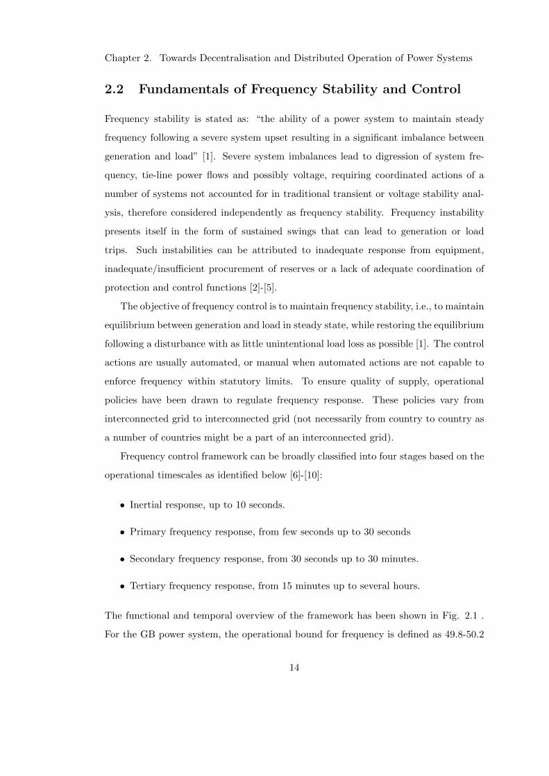
Frequency control framework can be broadly classified into four stages based on the
operational timescales as identified below [6]-[10]:
• Inertial response, up to 10 seconds.
• Primary frequency response, from few seconds up to 30 seconds
• Secondary frequency response, from 30 seconds up to 30 minutes.
• Tertiary frequency response, from 15 minutes up to several hours.
The functional and temporal overview of the framework has been shown in Fig. 2.1 .
For the GB power system, the operational bound for frequency is defined as 49.8-50.2
14

Chapter 2. Towards Decentralisation and Distributed Operation of Power Systems
Figure 2.1: Functional and temporal view of frequency control framework [10].
Hz, with the statutory limit set at 49.5-50.5 Hz. The maximum instantaneous deviation
in frequency from nominal is set at 0.8 Hz only for a duration of 60 s in response to
loss of largest infeed (1800 MW for GB) [11].
2.2.1 Inertial Response
Inertial response is the inherent response of synchronous generators to any power im-
balance, perceived as a change in frequency of the system. It is the release or the ab-
sorption of kinetic energy from/to the rotating mass of electrical machines connected
to the grid. This release/absorption of kinetic energy contributes towards limiting the
rate of change of frequency following an imbalance [12]. The kinetic energy stored in a
rotating machine (and its ability to limit the rate of change of frequency) is determined
by the inertia constant given by [13], [14]:
H =Jω2
0
2Sn(2.1)
where H is the inertia constant, J is the moment of inertia, ω0 is the rated angular
velocity of the machine and Sn is the rated power of the machine. Typically a power
system comprises a combination of generation units with different inertia constants
owing to diversity in type of fuel and the size of individual units. The equivalent
inertia constant (Heq) of a power system with n machines can be calculated as [15],
15
Chapter 2. Towards Decentralisation and Distributed Operation of Power Systems
[16]:
Heq =
∑ni=1Hi · Si∑ni=1 Si
(2.2)
The values of the inertia constants of power systems are typically in the range of 2 s to
9 s [17].
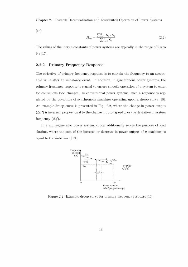
2.2.2 Primary Frequency Response
The objective of primary frequency response is to contain the frequency to an accept-
able value after an imbalance event. In addition, in synchronous power systems, the
primary frequency response is crucial to ensure smooth operation of a system to cater
for continuous load changes. In conventional power systems, such a response is reg-
ulated by the governors of synchronous machines operating upon a droop curve [18].
An example droop curve is presented in Fig. 2.2, where the change in power output
(∆P ) is inversely proportional to the change in rotor speed ω or the deviation in system
frequency (∆f).
In a multi-generator power system, droop additionally serves the purpose of load
sharing, where the sum of the increase or decrease in power output of n machines is
equal to the imbalance [19].
Figure 2.2: Example droop curve for primary frequency response [13].
16
Chapter 2. Towards Decentralisation and Distributed Operation of Power Systems
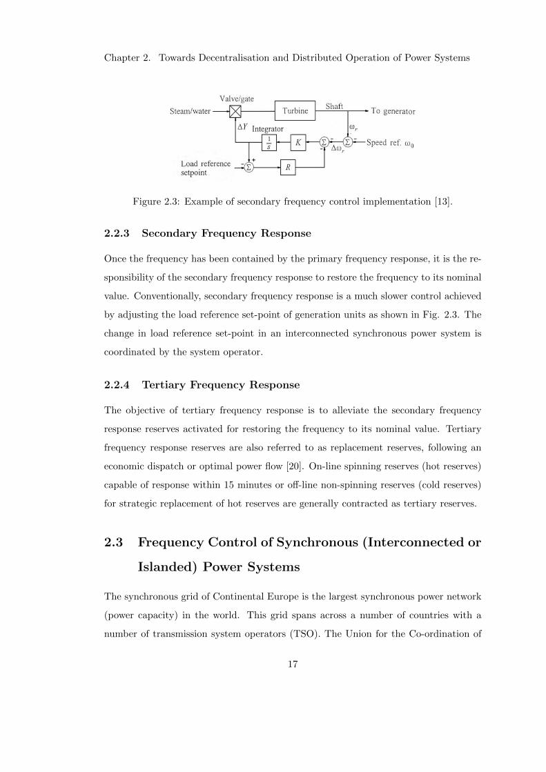
Figure 2.3: Example of secondary frequency control implementation [13].
2.2.3 Secondary Frequency Response
Once the frequency has been contained by the primary frequency response, it is the re-
sponsibility of the secondary frequency response to restore the frequency to its nominal
value. Conventionally, secondary frequency response is a much slower control achieved
by adjusting the load reference set-point of generation units as shown in Fig. 2.3. The
change in load reference set-point in an interconnected synchronous power system is
coordinated by the system operator.
2.2.4 Tertiary Frequency Response
The objective of tertiary frequency response is to alleviate the secondary frequency
response reserves activated for restoring the frequency to its nominal value. Tertiary
frequency response reserves are also referred to as replacement reserves, following an
economic dispatch or optimal power flow [20]. On-line spinning reserves (hot reserves)
capable of response within 15 minutes or off-line non-spinning reserves (cold reserves)
for strategic replacement of hot reserves are generally contracted as tertiary reserves.
2.3 Frequency Control of Synchronous (Interconnected or
Islanded) Power Systems
The synchronous grid of Continental Europe is the largest synchronous power network
(power capacity) in the world. This grid spans across a number of countries with a
number of transmission system operators (TSO). The Union for the Co-ordination of
17
Chapter 2. Towards Decentralisation and Distributed Operation of Power Systems
Transmission of Electricity (UCTE) has coordinated the operation and development
of the Continental Europe grid, ensuring reliable supply of electricity in Continental
Europe. UCTE operated since 1951, redefined itself as an association of TSO’s in 1999,
and was wounded up in 2009 with its responsibilities handed over to European Network
of Transmission System Operators for Electricity (ENTSO-E). ENTSO-E is responsible
not only for the Continental Europe grid but harmonizes the operation of the European
Grids representing 43 TSO’s from 36 countries across Europe [21].
In a synchronous grid, the network frequency is a common physical parameter,
observable throughout the network. On one hand, the frequency of the network impacts
all the installations (generation and demand) of the network, while on the other hand,
all installations impact the frequency. Therefore, although a TSO is responsible for its
own region (the geographical region across which the transmission network is spread),
ensuring a stable frequency control process is a common task of all operators within
the synchronous grid and a precondition for secure operation of the network. This can
be achieved if:
• A well defined and organised structure for load frequency control (LFC) is devel-
oped.
• TSO’s are obliged to cooperate.
For this reason, ENTSO-E has drafted the Network Code for Load Frequency Control
and Reserves (LFCR) to ensure frequency stability. Some of the key enabling features
of the network code are [22]:
• harmonised quality targets
• harmonised operational procedures
• harmonised minimum requirements
This chapter provides a common European framework for the Load-Frequency Con-
trol processes by setting technical requirements for the technical control structure and
the according responsibilities of the TSOs.
18
Chapter 2. Towards Decentralisation and Distributed Operation of Power Systems
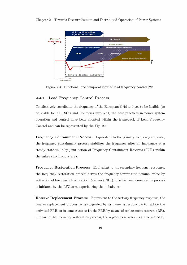
Figure 2.4: Functional and temporal view of load frequency control [22].
2.3.1 Load Frequency Control Process
To effectively coordinate the frequency of the European Grid and yet to be flexible (to
be viable for all TSO’s and Countries involved), the best practices in power system
operation and control have been adopted within the framework of Load-Frequency
Control and can be represented by the Fig. 2.4:
Frequency Containment Process: Equivalent to the primary frequency response,
the frequency containment process stabilizes the frequency after an imbalance at a
steady state value by joint action of Frequency Containment Reserves (FCR) within
the entire synchronous area.
Frequency Restoration Process: Equivalent to the secondary frequency response,
the frequency restoration process drives the frequency towards its nominal value by
activation of Frequency Restoration Reserves (FRR). The frequency restoration process
is initiated by the LFC area experiencing the imbalance.
Reserve Replacement Process: Equivalent to the tertiary frequency response, the
reserve replacement process, as is suggested by its name, is responsible to replace the
activated FRR, or in some cases assist the FRR by means of replacement reserves (RR).
Similar to the frequency restoration process, the replacement reserves are activated by
19
Chapter 2. Towards Decentralisation and Distributed Operation of Power Systems
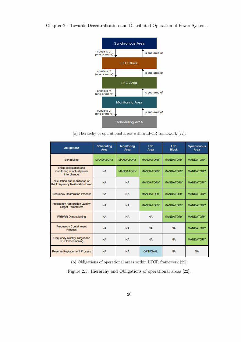
(a) Hierarchy of operational areas within LFCR framework [22].
(b) Obligations of operational areas within LFCR framework [22].
Figure 2.5: Hierarchy and Obligations of operational areas [22].
20
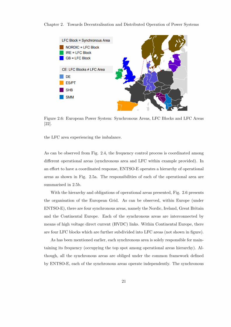
Chapter 2. Towards Decentralisation and Distributed Operation of Power Systems
Figure 2.6: European Power System: Synchronous Areas, LFC Blocks and LFC Areas[22].
the LFC area experiencing the imbalance.
As can be observed from Fig. 2.4, the frequency control process is coordinated among
different operational areas (synchronous area and LFC within example provided). In
an effort to have a coordinated response, ENTSO-E operates a hierarchy of operational
areas as shown in Fig. 2.5a. The responsibilities of each of the operational area are
summarised in 2.5b.
With the hierarchy and obligations of operational areas presented, Fig. 2.6 presents
the organisation of the European Grid. As can be observed, within Europe (under
ENTSO-E), there are four synchronous areas, namely the Nordic, Ireland, Great Britain
and the Continental Europe. Each of the synchronous areas are interconnected by
means of high voltage direct current (HVDC) links. Within Continental Europe, there
are four LFC blocks which are further subdivided into LFC areas (not shown in figure).
As has been mentioned earlier, each synchronous area is solely responsible for main-
taining its frequency (occupying the top spot among operational areas hierarchy). Al-
though, all the synchronous areas are obliged under the common framework defined
by ENTSO-E, each of the synchronous areas operate independently. The synchronous
21
Chapter 2. Towards Decentralisation and Distributed Operation of Power Systems
Frequency
Containment
Process
Frequency
Restoration
Process
Reserve
Replacement
Process
Frequency
Response
Services
Reserve
Services
Primary
Frequency Control
Secondary
Frequency Control
Tertiary
Frequency Control
ENTSO-E
LFCR
GB
Balancing
Services
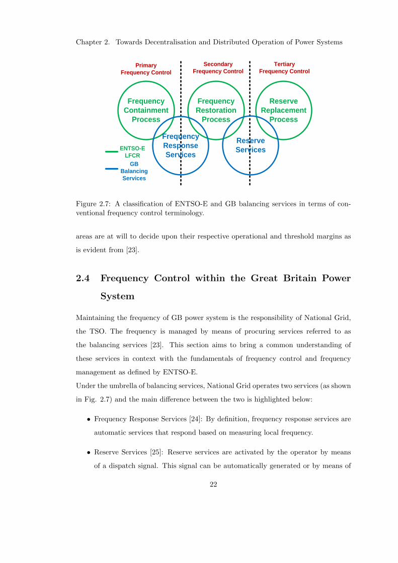
Figure 2.7: A classification of ENTSO-E and GB balancing services in terms of con-ventional frequency control terminology.
areas are at will to decide upon their respective operational and threshold margins as
is evident from [23].
2.4 Frequency Control within the Great Britain Power
System
Maintaining the frequency of GB power system is the responsibility of National Grid,
the TSO. The frequency is managed by means of procuring services referred to as
the balancing services [23]. This section aims to bring a common understanding of
these services in context with the fundamentals of frequency control and frequency
management as defined by ENTSO-E.
Under the umbrella of balancing services, National Grid operates two services (as shown
in Fig. 2.7) and the main difference between the two is highlighted below:
• Frequency Response Services [24]: By definition, frequency response services are
automatic services that respond based on measuring local frequency.
• Reserve Services [25]: Reserve services are activated by the operator by means
of a dispatch signal. This signal can be automatically generated or by means of
22

Chapter 2. Towards Decentralisation and Distributed Operation of Power Systems
Ba
lan
cin
g S
erv
ice
s Frequency
Response Services
Reserve Services
Mandatory Frequency
Response
Firm Frequency
Response
Demand Turn-Up
Balancing Mechanism
Start-Up
Short Term Operating
Reserves
Fast Reserve
Frequency
Containment Process
Frequency
Restoration Process
Reserve Replacement
Process
EN
TS
O-E
LF
CR
Figure 2.8: A mapping of GB balancing services to ENTSO-E LFCR (by means ofobjective of service).
manual intervention.
In Fig. 2.8, the frequency control objectives towards which the above services contribute
to are represented. As can be observed, the frequency response services contribute to
the objectives of frequency containment process and frequency restoration process while
the reserve services contribute to the objectives of frequency restoration process and
reserve replacement process. The following two sub-sections present the two services
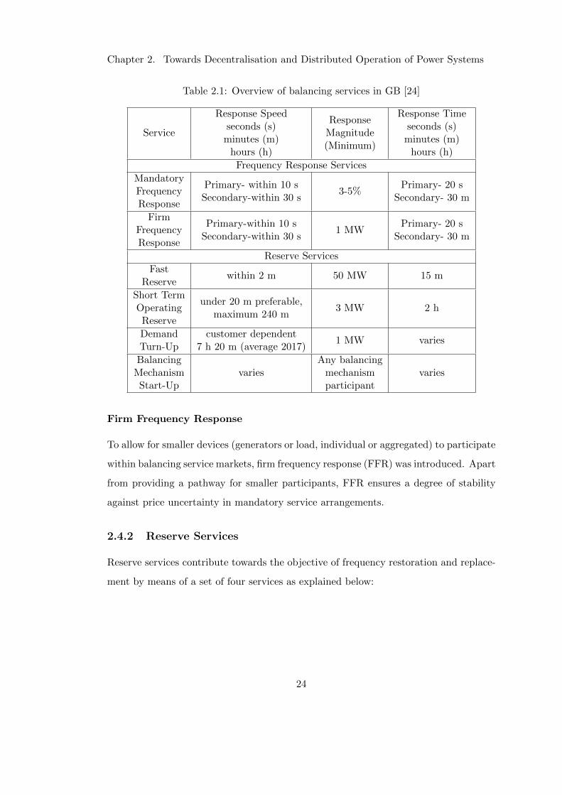
briefly with the technical requirements summarised in Table 2.1.
2.4.1 Frequency Response Services
As explained earlier, frequency response services contribute towards the objective of
frequency containment (including regulation) and restoration by means of a set of two
services as explained below:
Mandatory Frequency Response
The automatic change in active power in response to change in frequency is referred
to as the mandatory frequency response. This is a requirement by the grid code for
generators (usually greater than 30 MW).
23
Chapter 2. Towards Decentralisation and Distributed Operation of Power Systems
Table 2.1: Overview of balancing services in GB [24]
Service
Response Speedseconds (s)
minutes (m)hours (h)
ResponseMagnitude(Minimum)
Response Timeseconds (s)
minutes (m)hours (h)
Frequency Response Services
MandatoryFrequencyResponse
Primary- within 10 sSecondary-within 30 s
3-5%Primary- 20 s
Secondary- 30 m
FirmFrequencyResponse
Primary-within 10 sSecondary-within 30 s
1 MWPrimary- 20 s
Secondary- 30 m
Reserve Services
FastReserve
within 2 m 50 MW 15 m
Short TermOperatingReserve
under 20 m preferable,maximum 240 m
3 MW 2 h
DemandTurn-Up
customer dependent7 h 20 m (average 2017)
1 MW varies
BalancingMechanismStart-Up
variesAny balancing
mechanismparticipant
varies
Firm Frequency Response
To allow for smaller devices (generators or load, individual or aggregated) to participate
within balancing service markets, firm frequency response (FFR) was introduced. Apart
from providing a pathway for smaller participants, FFR ensures a degree of stability
against price uncertainty in mandatory service arrangements.
2.4.2 Reserve Services
Reserve services contribute towards the objective of frequency restoration and replace-
ment by means of a set of four services as explained below:
24
Chapter 2. Towards Decentralisation and Distributed Operation of Power Systems
Fast Reserve
The rapid and reliable delivery of active power by means of increasing output from
generating devices or reducing consumption from demand sources is referred to as Fast
Reserve service.
Short Term Operating Reserves
The delivery of active power by means of increasing output from generating devices or
reducing consumption from demand sources only at certain times of the day is referred
to as short term operating reserve. This service is intended to cater for forecast errors
and unforeseen generation unavailability.
Demand Turn-Up
The demand turn up service encourages large customers (load or generation) to ei-
ther increase demand or reduce generation at times of high renewable output and low
national demand. This service is usually requested overnight and during weekend af-
ternoons in summer.
Balancing Mechanism (BM) Start-Up
This service can be regarded as the precautionary (or anticipatory) service and is made
up of two elements: (i) BM start up where generation units are brought to a state at
which they will be able to synchronize to the network within 89 minutes, and (ii) hot
standby where the generation unit is capable to synchronize with the grid.
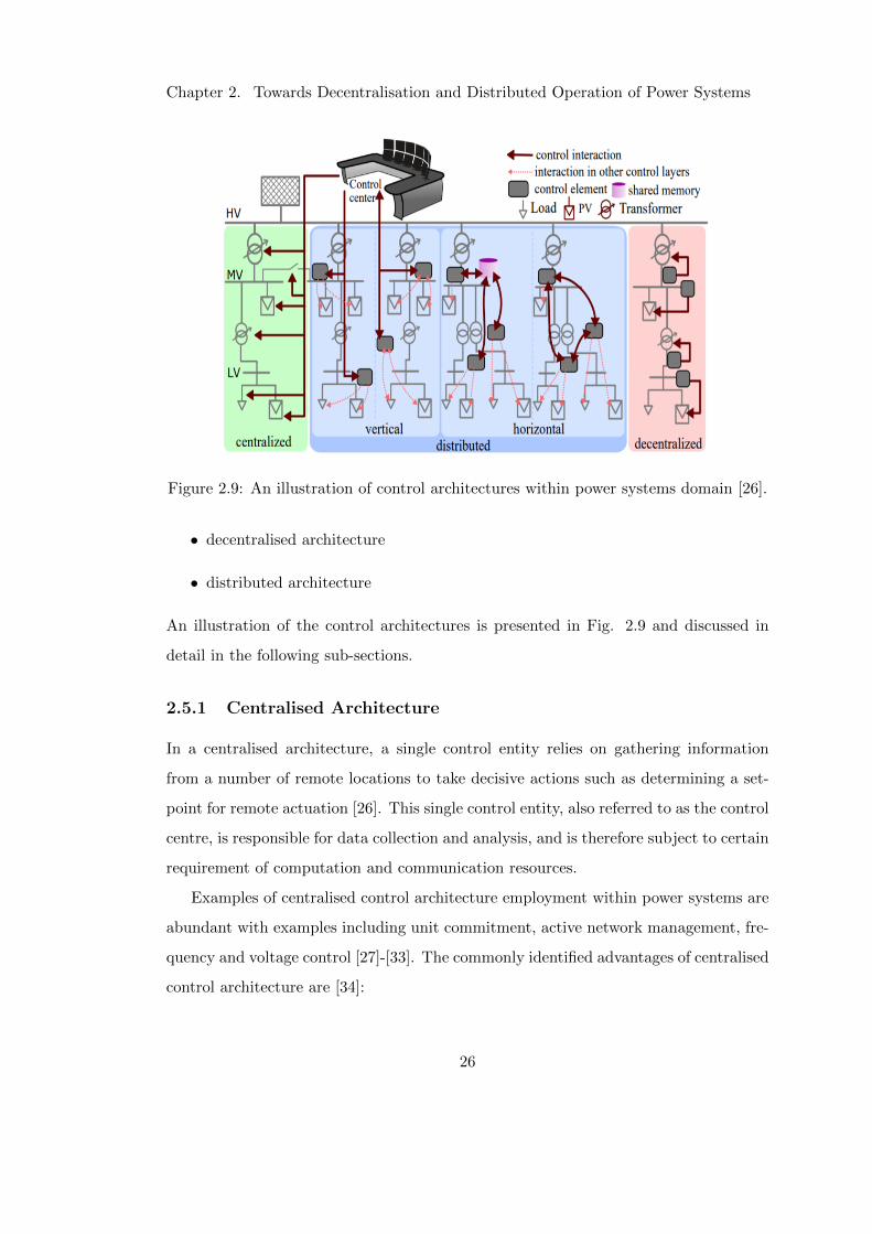
2.5 Control Architectures
The spatial distribution and function of the entities, such as the control elements and
instrumentation, within a control system and the relations between those entities can
be referred to as the control architecture [26]. The control architectures within power
systems domain can be classified into three:
• centralised architecture
25
Chapter 2. Towards Decentralisation and Distributed Operation of Power Systems
Figure 2.9: An illustration of control architectures within power systems domain [26].
• decentralised architecture
• distributed architecture
An illustration of the control architectures is presented in Fig. 2.9 and discussed in
detail in the following sub-sections.
2.5.1 Centralised Architecture
In a centralised architecture, a single control entity relies on gathering information
from a number of remote locations to take decisive actions such as determining a set-
point for remote actuation [26]. This single control entity, also referred to as the control
centre, is responsible for data collection and analysis, and is therefore subject to certain
requirement of computation and communication resources.
Examples of centralised control architecture employment within power systems are
abundant with examples including unit commitment, active network management, fre-
quency and voltage control [27]-[33]. The commonly identified advantages of centralised
control architecture are [34]:
26
Chapter 2. Towards Decentralisation and Distributed Operation of Power Systems
• A centralised control architecture is simple to implement, comprehend and there-
fore also easy to maintain.
• A centralised control architecture enables complete observability, i.e. ensures the
availability of overall system state or overall system knowledge.
• Owing to the comprehensive knowledge of the system, a centralised control archi-
tecture enables implementation of controls that guarantee fairness and optimality.
On the other hand, the disadvantages of a centralised control architecture can be sum-
marised as [34]:
• As all the intelligent computation is at one location within one entity (control
centre), centralised control architectures are susceptible to single point of failure.
• The responsiveness, in other words the performance, of a centralised control archi-
tecture is highly dependent upon the computational resources and communication
architecture employed.
• The scalability of centralised control architectures are limited by the computa-
tional resources and communication architecture employed.
2.5.2 Decentralised Architecture
In a decentralised architecture, multiple control entities are jointly responsible for a
common objective, intended to take decisive actions independently of each other based
on local observables only [26]. The most common decentralised control for power system
is the primary frequency control via active power/frequency droop [35] or the local
voltage control via reactive power/voltage droop [36].
The reliance of decentralised control on local observables voids any need for com-
munication, thereby offering a form of resilience. This resilience is the reason for de-
centralised control often being employed for system critical services such as primary
frequency control, the first line of defence in case of large system contingencies, and
over current protection against faults within the network.
27
Chapter 2. Towards Decentralisation and Distributed Operation of Power Systems
D-V-D D-V-I
D-H-C D-H-P
Figure 2.10: An illustration of distributed control architectures within power systemsdomain [26].
Coordination within decentralised control algorithms is difficult due to the lack
of interaction among the entities involved. A system level coordination in primary
frequency control is achieved due to the physical property of the controlled process,
i.e., the steady-state frequency is same irrespective of where it is measured within
a network and therefore acting as means of information. As the decisions taken by
decentralised control are under partial knowledge of the system, it is also difficult
to achieve optimality and to ensure fairness. An attempt to improve optimality in
decentralised controls by means of local signal processing and employment of improved
process models is reported in [37], while parametrisation of local control parameters by
addition of topological information to achieve fairness is reported in [38].
Although the mass deployment of such control is easy, owing to dependence on
local observables only, design and maintenance of such control algorithms are often
more challenging.
28
Chapter 2. Towards Decentralisation and Distributed Operation of Power Systems
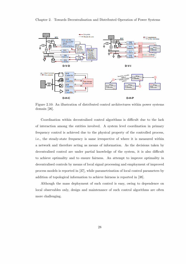
2.5.3 Distributed Architecture
A distributed control architecture can be observed as a hybrid (some form of combina-
tion of centralised and decentralised) where a common control objective is decomposed
and delegated to independent control elements. Depending upon how the common
control objective is decomposed and delegated, the distributed architectures can be
classified into two [26]:
Distributed Vertical (D-V): When the common control objective is decomposed
and delegated in a way such that the decision of one control element is imposed on the
other, the architecture is referred to as D-V. The D-V architecture imposes a level of
hierarchy among the participating control elements. In such an architecture, the low
level controllers (decentralised controllers) do lose a degree of freedom, however, owing
to the characteristics of hierarchy (a form of centralisation), more optimal solutions are
feasible. Examples are [39]-[42].
Distributed Horizontal (D-H): When the control responsibilities of all the con-
trol elements involved are symmetrical such that there is no hierarchy among them,
the control architecture is referred to as D-H. A system level coordination with such an
architecture is difficult and although the controllers have a higher degree of freedom,
the solutions are not necessarily optimal. Examples are [43]-[46].
Based on the type of information exchange between the control elements, each of the
two distributed architectures can be further sub-classified into two:
Distributed Vertical Determinate (D-V-D): An example representation of D-V-
D architecture is presented in Fig. 2.10. As can be observed, in a D-V-D architecture,
there is a hierarchical information collection and a centralised decision making. The
lower-level control elements do not have a say in the deterministic decision taken at the
higher level control. Examples are [41] and [42].
29
Chapter 2. Towards Decentralisation and Distributed Operation of Power Systems
Distributed Vertical Iterative (D-V-I): Similar to the D-V-D architecture, in
a D-V-I architecture, the information gathering is hierarchical; however, the lower-
level controllers can negotiate the decision brought by the higher-level controller, and
therefore incorporating the term iterative in its name. The negotiation between the
different control levels is captured by bi-directional arrows in 2.10. Examples are [39],
[40] and [47].
Distributed Horizontal Centralised (D-H-C): With the control responsibility
of all control elements involved being symmetrical, if an additional centralised entity
exists that coordinates the information exchange between the control elements, the
architecture is referred to as D-H-C (as shown in Fig 2.10). While the existence of
a centralised entity makes the architecture more susceptible to a single point of fail-
ure, it reduces the burden on communications infrastructure, making it more scalable.
Examples are [43] and [44].
Distributed Horizontal Peer to Peer (D-H-P): The final architecture is the D-
H-P, a fully distributed architecture, where the information exchange is wholly between
the controllers, peer to peer (P2P). Examples are [45] and [46]. The burden imposed
on communications infrastructure by the P2P information exchange can limit the scal-
ability of such architectures. In recent literature, graph theory has been utilised to
enforce sparse communication within a set of controllers, while ensuring that the con-
trol objective is achieved.
2.5.4 An Architectural Analysis of Present Day Frequency Control of
Power Systems
Generally in power systems, any control problem is mathematically decomposed into
three time-dependent cascaded layers referred to as the primary, secondary, and tertiary
control layers [48]. More often, the following architectural view is widely assumed for
the three layers:
• Primary ⇒ Decentralised
30
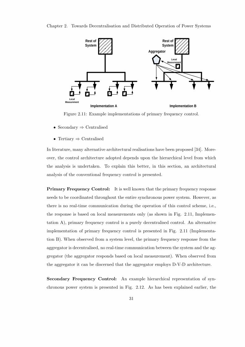
Chapter 2. Towards Decentralisation and Distributed Operation of Power Systems
Local
Measurement
Local
Measurement
Aggregator
Implementation A Implementation B
Rest of
System
Rest of
System
Figure 2.11: Example implementations of primary frequency control.
• Secondary ⇒ Centralised
• Tertiary ⇒ Centralised
In literature, many alternative architectural realisations have been proposed [34]. More-
over, the control architecture adopted depends upon the hierarchical level from which
the analysis is undertaken. To explain this better, in this section, an architectural
analysis of the conventional frequency control is presented.
Primary Frequency Control: It is well known that the primary frequency response
needs to be coordinated throughout the entire synchronous power system. However, as
there is no real-time communication during the operation of this control scheme, i.e.,
the response is based on local measurements only (as shown in Fig. 2.11, Implemen-
tation A), primary frequency control is a purely decentralised control. An alternative
implementation of primary frequency control is presented in Fig. 2.11 (Implementa-
tion B). When observed from a system level, the primary frequency response from the
aggregator is decentralised, no real-time communication between the system and the ag-
gregator (the aggregator responds based on local measurement). When observed from
the aggregator it can be discerned that the aggregator employs D-V-D architecture.
Secondary Frequency Control: An example hierarchical representation of syn-
chronous power system is presented in Fig. 2.12. As has been explained earlier, the
31
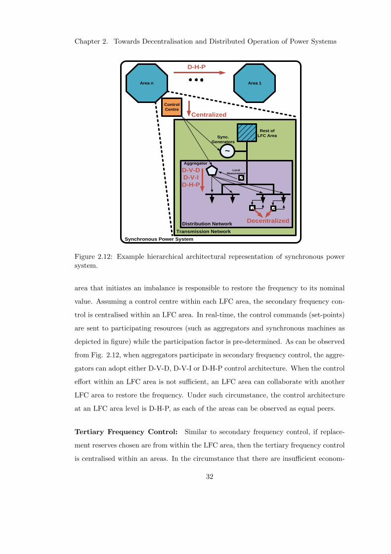
Chapter 2. Towards Decentralisation and Distributed Operation of Power Systems
Local
Measurement
Aggregator
Area 1Area n
Synchronous Power System
Control
Centre
Distribution Network
Transmission Network
~
Rest of
LFC Area
D-H-P
Decentralized
D-V-D
D-V-I
D-H-P
Centralized
Sync.
Generators
Figure 2.12: Example hierarchical architectural representation of synchronous powersystem.
area that initiates an imbalance is responsible to restore the frequency to its nominal
value. Assuming a control centre within each LFC area, the secondary frequency con-
trol is centralised within an LFC area. In real-time, the control commands (set-points)
are sent to participating resources (such as aggregators and synchronous machines as
depicted in figure) while the participation factor is pre-determined. As can be observed
from Fig. 2.12, when aggregators participate in secondary frequency control, the aggre-
gators can adopt either D-V-D, D-V-I or D-H-P control architecture. When the control
effort within an LFC area is not sufficient, an LFC area can collaborate with another
LFC area to restore the frequency. Under such circumstance, the control architecture
at an LFC area level is D-H-P, as each of the areas can be observed as equal peers.
Tertiary Frequency Control: Similar to secondary frequency control, if replace-
ment reserves chosen are from within the LFC area, then the tertiary frequency control
is centralised within an areas. In the circumstance that there are insufficient econom-
32
Chapter 2. Towards Decentralisation and Distributed Operation of Power Systems
ical replacement reserves within an area, the D-H-P architecture is adopted between
the LFC areas.
2.6 Transformation of the Great Britain Power System
For the past several decades, power systems have been characterised as “unidirectional”,
with a small number of relatively large power plants feeding power to end consumers.
End consumers remained fairly passive with no interaction with power delivery mecha-
nism. In the recent years, power systems have been experiencing a number of changes in
generation and consumption that have begun to set a trend internationally and present
a challenge to the traditional “unidirectional” view of the power system. In this section,
these changes will be presented for the GB power system categorically, summarising
views and foresights from the Institution of Engineering Technology (IET) reported in
a position statement towards a 2030 GB power system [49] and by National Grid re-
ported in the Future Energy Scenarios (FES) towards a 2050 power system [50]. These
categories presented below are considered as the challenges power networks face in the
circumstance of the transition.
Increasing Renewable Generation Penetration: About 34% (34GW) of the in-
stalled capacity (100GW) within the GB grid is renewable generation (as of 2016) and
is expected to grow rapidly with increasing pressure to meet the climate change ob-
jectives. Based on the two degree scenario of the FES, it is expected that there will
be 223% increase in capacity of renewable generation. This increased capacity will
represent 60% (110GW) of the total generation capacity (∼ 184GW) in 2050. Among
the different types of renewable resources, wind is expected to dominate in terms of
the magnitude of installation (50 GW of wind installation compared to 44 GW of solar
installation) however solar is expected to see the highest percentage (400%) increase.
Increasing Distributed Generation Penetration: In 2016, the reported installed
capacity from distributed generation (generation installed at distribution level rather
than transmission level) was 27% (∼ 26GW) of total installed capacity. In 2050, an
33
Chapter 2. Towards Decentralisation and Distributed Operation of Power Systems
increase to a total of 93 GW is expected, representing 50% of the total installed ca-
pacity. This expected increase will be from a mix of generation sources. Interestingly,
24GW of small-scale thermal generation is expected to be distributed within the grid.
The majority of the 44 GW solar penetration mentioned earlier will also be at the
distribution level. Energy storage (larger dedicated storage units or the battery within
an electric vehicle) is expected to be part of the distributed generation.
Changing Demand Profile: In 2050, electricity peak demand can be expected to
increase to 85GW from around 60GW in 2016. Electric vehicles are expected to see a
steady growth, owing to increasing customer acceptance and technology improvements,
with about one million cars in 2020 and more than nine million by 2030+. As per es-
timation, without coordinated smart charging mechanism, this increasing penetration
could directly translate to an increase in 8 GW of demand at peak times. With chang-
ing weather patterns, it is further anticipated that with an increase in temperature,
peak demand in summer could raise to levels as seen in winter due to increase in air
conditioning load. The increase in peak demand is not the only expected change, a
change in peak period is anticipated with increasing penetration of distributed genera-
tion. For example, in a future scenario with large percentage of residential consumers
with photovoltaic (PV) rooftops, sun shining in a summer month can lead to signifi-
cant reduction in transmission demand. This would set a new trend of noon time being
considered as the time with least demand (as compared to early mornings today).
Demand Side Management: In the present day power system, although there is
an increasing interest in utilising demand side to assist the network, this has been
limited to larger industrial demand. This is evident from the preference of 100kW or
greater capacity participants by the twenty three aggregators within the GB network.
Effectively, there is 0% penetration of home energy management in broad terms, i.e.
all the domestic residential demand is passive. With the mass roll-out of smart meters,
95% of UK homes are expected to be capable of providing real-time information for
active demand response by 2020. It is estimated that with only half of the installed
smart meters linked to an energy management system, there will be about 15 million
34
Chapter 2. Towards Decentralisation and Distributed Operation of Power Systems
units available for utilisation by 2030.
Modern Control and Automation: The advancements in information and com-
munication technologies (ICT) and automation technologies will bring more opportu-
nities (and challenges at the same time) to the traditional controls employed within
the present day power system. For example, in present day GB network 10-15 large
generating units connected at transmission level operate in frequency control mode,
maintaining the frequency of the network. In the future, most electrical devices are
expected to be interconnected and controllable via a phone or an aggregator. Although
the extent to how much flexibility this can deliver is unclear, an example representation
is the availability of 600,000 units available for assisting in frequency control if only
10% of interconnected devices are utilised. In a similar manner, about 10,000 devices
are responsible for voltage regulation within the present day distribution network under
the umbrella of distribution network automation. In the future, there will be 900,000
units capable of participation in voltage regulation within the distribution network, a
90% increase.
2.7 Analysing the Impact of Transformation
In this section, the impact of the transformations of GB power system summarised in
the previous section will be analysed with respect to the following three categories:
• System Frequency Response
• System Stability
• System Controllability
2.7.1 System Frequency Response
A majority of the renewable generation resources, such as PV and wind, are intercon-
nected to the grid through power electronics. As inertia of a system is derived from
energy stored in rotating masses within the network, the renewable resources effectively
35
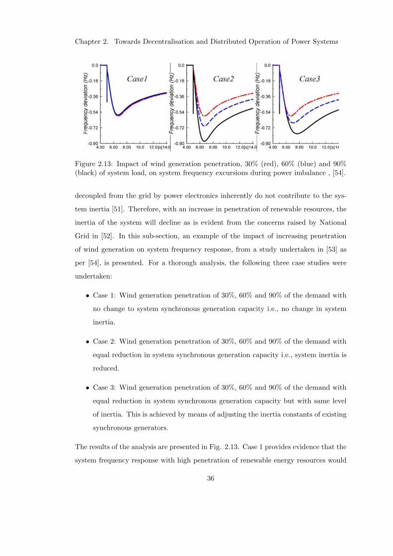
Chapter 2. Towards Decentralisation and Distributed Operation of Power Systems
Figure 2.13: Impact of wind generation penetration, 30% (red), 60% (blue) and 90%(black) of system load, on system frequency excursions during power imbalance , [54].
decoupled from the grid by power electronics inherently do not contribute to the sys-
tem inertia [51]. Therefore, with an increase in penetration of renewable resources, the
inertia of the system will decline as is evident from the concerns raised by National
Grid in [52]. In this sub-section, an example of the impact of increasing penetration
of wind generation on system frequency response, from a study undertaken in [53] as
per [54], is presented. For a thorough analysis, the following three case studies were
undertaken:
• Case 1: Wind generation penetration of 30%, 60% and 90% of the demand with
no change to system synchronous generation capacity i.e., no change in system
inertia.
• Case 2: Wind generation penetration of 30%, 60% and 90% of the demand with
equal reduction in system synchronous generation capacity i.e., system inertia is
reduced.
• Case 3: Wind generation penetration of 30%, 60% and 90% of the demand with
equal reduction in system synchronous generation capacity but with same level
of inertia. This is achieved by means of adjusting the inertia constants of existing
synchronous generators.
The results of the analysis are presented in Fig. 2.13. Case 1 provides evidence that the
system frequency response with high penetration of renewable energy resources would
36
Chapter 2. Towards Decentralisation and Distributed Operation of Power Systems
be unaffected if the capacity of synchronous generation within the system remains un-
changed. Case 2 provides the evidence of the impact of reduction of inertia of the
network on the system frequency response. The reduction in synchronous generation
capacity does not only impact the rate of change of frequency but also the frequency
nadir. Case 3 provides evidence that the increasing penetration of renewable gener-
ation and simultaneous reduction of synchronous generation capacity, even without
decreasing the system inertia, degrades the frequency response of the system (in terms
of frequency nadir).
From the above study it becomes clear that increasing penetration of renewable
generation sources, the decreasing penetration of synchronous generation and the con-
sequent decrease in system inertia deteriorates the system frequency response. This
deterioration in frequency response represents an emerging frequency control challenge
faced by system operators around the world. For example, in a study undertaken by
Australian Energy Market Operator (AEMO), the RoCoF level is expected to increase
with the expected change in generation mix (i.e., with rapid uptake of non-synchronous
generation) [55]. With the new expected levels of RoCoF in 2021-2022, it is anticipated
that there would be less than two seconds for primary frequency control actions to
arrest the frequency before it declines below the containment band defined by Fre-
quency Operating Standard (FOS) [56]. The two seconds range is much faster than
the typically observed response time of synchronous generators. Therefore, it can be
said that, the decreasing inertia in the network imposes new time restrictions (or re-
quirements) on existing services. As existing services are basically classified in terms
of time of response, the previous statement can be rephrased as: the decreasing inertia
in the network imposes new time restrictions (or requirements) therefore requiring new
services to be defined.
The need to reduce the RoCoF has motivated the development of virtual syn-
chronous generators (VSGs). The term VSG refers to a converter control approach
that enables emulation of inertial response of synchronous machines over short periods
of time, often referred to as virtual, synthetic or emulated inertia [57]-[59]. Typi-
cally, any power electronic interfaced distributed generation with appropriate control
37
Chapter 2. Towards Decentralisation and Distributed Operation of Power Systems
can help improve the dynamic response of the system (i.e., help improve RoCoF). Al-
though in recent literature a number of works have proposed novel synthetic-inertial
control approaches [60]-[65], in practice synthetic inertia is commercially unavailable
[66]. Furthermore, as reported in [66], virtual inertia emulation is feasible within power
networks with high inertia, but it becomes increasingly challenging to obtain an appro-
priate transient response in low inertia circumstances. In addition, system operators
realize the adaptable nature of power electronic interfaced devices can yield a wider
range of responses and enforcing only inertial response from such devices can be limiting
and can curb further developments.
Therefore the need for faster acting service provision has been realised by the sys-
tem operators. In this context, the inertial response from power electronic interfaced
devices is encompassed within the umbrella of fast acting service provision but not
limited to it. In essence, system operators are looking for fast response in the entire
spectrum of frequency control mechanisms as is evident from the pilots and plans of
some international system operators summarised below [67]:
• In Canada, Hydro-Quebec has mandated all wind generation connecting to its
network to provide inertial response [68]. Ontario and Brazil have more recently
introduced similar mandatory requirements[69], [70].
• In GB, National Grid has planned to pilot one second Enhanced Frequency Re-
sponse service to be delivered by batteries [71]. This service is based on droop
but with a narrow dead band, similar to primary frequency response delivered by
synchronous governors.
• In the USA, PJM has employed batteries and flywheels for dynamic regulation
services, responding to SFC signals. Participants are paid a price proportional to
their speed of response, encouraging faster response [72].
• In New Zealand, a one second service is already delivered by demand response
towards objective of primary frequency control [73].
• In Texas, Electric Reliability Council of Texas (ERCOT) proposed a half second
38
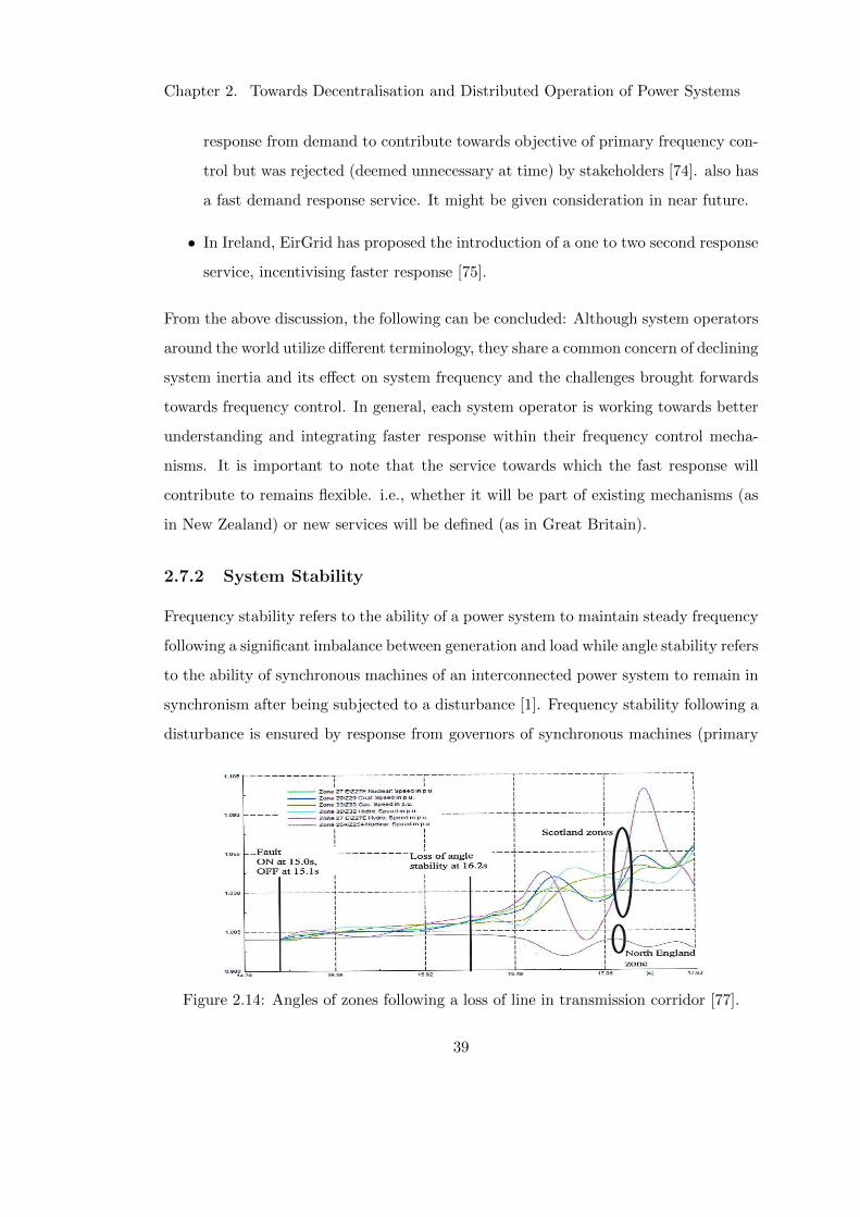
Chapter 2. Towards Decentralisation and Distributed Operation of Power Systems
response from demand to contribute towards objective of primary frequency con-
trol but was rejected (deemed unnecessary at time) by stakeholders [74]. also has
a fast demand response service. It might be given consideration in near future.
• In Ireland, EirGrid has proposed the introduction of a one to two second response
service, incentivising faster response [75].
From the above discussion, the following can be concluded: Although system operators
around the world utilize different terminology, they share a common concern of declining
system inertia and its effect on system frequency and the challenges brought forwards
towards frequency control. In general, each system operator is working towards better
understanding and integrating faster response within their frequency control mecha-
nisms. It is important to note that the service towards which the fast response will
contribute to remains flexible. i.e., whether it will be part of existing mechanisms (as
in New Zealand) or new services will be defined (as in Great Britain).
2.7.2 System Stability
Frequency stability refers to the ability of a power system to maintain steady frequency
following a significant imbalance between generation and load while angle stability refers
to the ability of synchronous machines of an interconnected power system to remain in
synchronism after being subjected to a disturbance [1]. Frequency stability following a
disturbance is ensured by response from governors of synchronous machines (primary
Figure 2.14: Angles of zones following a loss of line in transmission corridor [77].
39
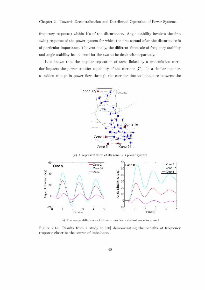
Chapter 2. Towards Decentralisation and Distributed Operation of Power Systems
frequency response) within 10s of the disturbance. Angle stability involves the first
swing response of the power system for which the first second after the disturbance is
of particular importance. Conventionally, the different timescale of frequency stability
and angle stability has allowed for the two to be dealt with separately.
It is known that the angular separation of areas linked by a transmission corri-
dor impacts the power transfer capability of the corridor [76]. In a similar manner,
a sudden change in power flow through the corridor due to imbalance between the
(a) A representation of 36 zone GB power system
(b) The angle difference of three zones for a disturbance in zone 1
Figure 2.15: Results from a study in [78] demonstrating the benefits of frequencyresponse closer to the source of imbalance.
40
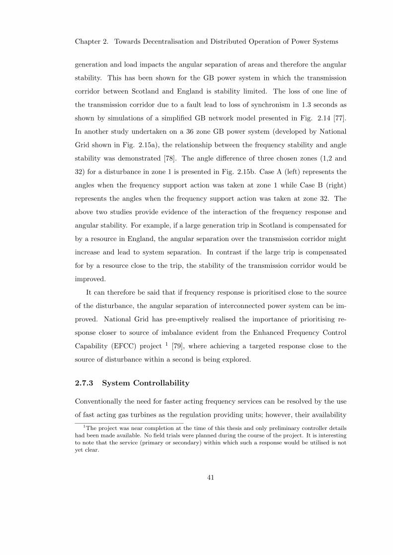
Chapter 2. Towards Decentralisation and Distributed Operation of Power Systems
generation and load impacts the angular separation of areas and therefore the angular
stability. This has been shown for the GB power system in which the transmission
corridor between Scotland and England is stability limited. The loss of one line of
the transmission corridor due to a fault lead to loss of synchronism in 1.3 seconds as
shown by simulations of a simplified GB network model presented in Fig. 2.14 [77].
In another study undertaken on a 36 zone GB power system (developed by National
Grid shown in Fig. 2.15a), the relationship between the frequency stability and angle
stability was demonstrated [78]. The angle difference of three chosen zones (1,2 and
32) for a disturbance in zone 1 is presented in Fig. 2.15b. Case A (left) represents the
angles when the frequency support action was taken at zone 1 while Case B (right)
represents the angles when the frequency support action was taken at zone 32. The
above two studies provide evidence of the interaction of the frequency response and
angular stability. For example, if a large generation trip in Scotland is compensated for
by a resource in England, the angular separation over the transmission corridor might
increase and lead to system separation. In contrast if the large trip is compensated
for by a resource close to the trip, the stability of the transmission corridor would be
improved.
It can therefore be said that if frequency response is prioritised close to the source
of the disturbance, the angular separation of interconnected power system can be im-
proved. National Grid has pre-emptively realised the importance of prioritising re-
sponse closer to source of imbalance evident from the Enhanced Frequency Control
Capability (EFCC) project 1 [79], where achieving a targeted response close to the
source of disturbance within a second is being explored.
2.7.3 System Controllability
Conventionally the need for faster acting frequency services can be resolved by the use
of fast acting gas turbines as the regulation providing units; however, their availability
1The project was near completion at the time of this thesis and only preliminary controller detailshad been made available. No field trials were planned during the course of the project. It is interestingto note that the service (primary or secondary) within which such a response would be utilised is notyet clear.
41
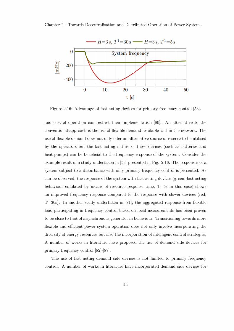
Chapter 2. Towards Decentralisation and Distributed Operation of Power Systems
Figure 2.16: Advantage of fast acting devices for primary frequency control [53].
and cost of operation can restrict their implementation [80]. An alternative to the
conventional approach is the use of flexible demand available within the network. The
use of flexible demand does not only offer an alternative source of reserve to be utilised
by the operators but the fast acting nature of these devices (such as batteries and
heat-pumps) can be beneficial to the frequency response of the system. Consider the
example result of a study undertaken in [53] presented in Fig. 2.16. The responses of a
system subject to a disturbance with only primary frequency control is presented. As
can be observed, the response of the system with fast acting devices (green, fast acting
behaviour emulated by means of resource response time, T=5s in this case) shows
an improved frequency response compared to the response with slower devices (red,
T=30s). In another study undertaken in [81], the aggregated response from flexible
load participating in frequency control based on local measurements has been proven
to be close to that of a synchronous generator in behaviour. Transitioning towards more
flexible and efficient power system operation does not only involve incorporating the
diversity of energy resources but also the incorporation of intelligent control strategies.
A number of works in literature have proposed the use of demand side devices for
primary frequency control [82]-[87].
The use of fast acting demand side devices is not limited to primary frequency
control. A number of works in literature have incorporated demand side devices for
42
Chapter 2. Towards Decentralisation and Distributed Operation of Power Systems
secondary frequency control and have brought forwards the advantages of the fast
acting nature of such devices. For example, in [88] and [89], it has been shown that
the utilisation of a utility scale battery energy storage system (BESS) in conjunction
with conventional generators (CG) improves the AGC performance of the CGs. In a
study that characterizes the effectiveness of utilising BESS for AGC compared to CGs,
it has been claimed that the utilisation of BESS reduces the regulation requirement
even when BESS constitute a small portion of total capacity [90]. This has also been
confirmed in studies conducted by [91]. Although the performance of AGC is improved
by utilising fast acting devices, the slow nature of AGC, due to ramp rate constraints
on CGs, does not allow for exploitation of the true potential of such devices.
An approach, already in use in the GB power system and referred to as frequency
control by demand management (FCDM) [92], provides an alternative means to exploit
the power ramping potential of fast acting devices. This approach is based on deter-
mining a frequency threshold for participating fast acting devices [93]. The amount of
reserves activated by such means is subtracted from the AGC regulation command. In
[94], it was shown that such an approach alleviates the burden on AGC and provides a
better frequency response. Bringing EFCC in context, it can be said that EFCC is an
improvement to the existing FCDM, extended to utilize faster responding devices with
responsibilisation. At present, only relatively large commercial customers participate in
FCDM and are activated by means of under-frequency relays while the market structure
for EFCC remains unclear. The dimensioning of FCDM reserves and the thresholds for
activation of FCDM reserves are carefully determined based on the system power fre-
quency characteristics. In the future, with high penetration of intermittent renewable
energy resources within the grid, the dimensioning of FCDM reserves and calculation of
thresholds for their activation will prove to be even more challenging as highly variable
system power frequency characteristics are anticipated. The opportunity of participat-
ing in FCDM will be extended to the large amount of flexibility foreseen to be available
within the grid (including domestic devices such as electric vehicles and heat pumps).
Devices interfaced by power electronics will have no difficulty in participating through
local measurements, however, some devices that inherently do not incorporate local
43
Chapter 2. Towards Decentralisation and Distributed Operation of Power Systems
observables may not be able to participate even with large amount of such devices may
be ICT enabled.
In other words, the large amount of distributed domestic flexibility within the net-
work will be available to participate through the traditional AGC (as it does not require
local measurements but requires ICT enabled devices). In [95]-[97], alternative struc-
tures for AGC and controls for fast acting devices to participate in such structures
have been proposed. This does play into the idea of utilising fast acting devices for a
wide spectrum of services (not just primary but secondary as well), however, as the
nature of AGC is centralised, the approach may not be able to operate under increased
number of participating units. This may be either due to the requirement of complex
communications network with two-way communication links or the requirement of a
powerful central controller to process large amount of data, both of which reduce over-
all system reliability and increases its sensitivity to failures [34]. The establishment
of the concept of demand side aggregators has facilitated the transition of AGC from
a centralised control approach to a distributed approach. In the process it has also
facilitated the participation of fast acting devices within AGC structures.
2.8 The Research Objectives
The analysis undertaken in the previous section affirms the challenges posed to conven-
tional approaches to frequency management under the certainty of changes expected
within the power systems around the world. To ensure the security of supply, following
requirements can be established:
• Frequency control approaches need to be faster acting.
• Frequency control approaches need to be locationally targeted.
• Frequency control approaches need to be able to incorporate the variety of devices
available within the network effectively.
Out of the three requirements identified, the most recently identified concept is the
need for incorporating locational information. Acknowledging this emerging need to
44
Chapter 2. Towards Decentralisation and Distributed Operation of Power Systems
incorporate locational information for a targeted response to a power system imbalance,
this thesis introduces the term “responsibilisation”:
“The prioritisation of remedial control measures electrically closer to the
source of the disturbance is referred to as responsibilisation”.
The introduction of the term is aimed at filling a gap in referring to an important
concept thereby supporting the drive towards the new paradigm of greater decentrali-
sation of power systems. With the review of fundamentals and practices of frequency
control presented, the requirements for frequency control approaches derived, and the
introduction of the term “responsibilisation”, the research questions to be addressed
by this thesis can be formulated as:
• Observing from a synchronous power system perspective, as every LFC area is
responsible to cater for its own imbalance, it can be said that responsibilisation is
incorporated within secondary frequency control implemented within the number
of LFC areas of the synchronous region. However, can its speed of response be
improved without jeopardising system stability?
• Primary frequency control’s operation at a much faster timescale than secondary
frequency control, where responsibilisation is conventionally in place, presents a
challenge for responsibilisation. Can effective decentralised method for responsi-
bilisation be developed for primary frequency control?
• The participation of demand side management in ancillary service provision is
proven in a number of energy markets, yet its full potential to benefit frequency
management, including the exploitation of fast power ramping capability of some
devices, is still undergoing research. Can the fast power ramping capability of
demand side devices be effectively harnessed?
2.9 Chapter Summary
In this chapter, the fundamentals of power system frequency control were presented fol-
lowed by frequency management within synchronous power system of Continental Eu-
45

Chapter 2. Towards Decentralisation and Distributed Operation of Power Systems
rope and GB. This chapter further introduced the concepts of centralised, decentralised
and distributed control architectures and presented an architectural analysis of present
day frequency control of power systems. By presenting the expected transformations of
GB power system in the near future, the impact of such system developments on sys-
tem frequency response, stability and controllability were discussed. From the analysis
of the impact, the emerging need to prioritize control measures close to the source of
imbalance events is acknowledged and the term responsibilisation is introduced. With
the discussion of the implications of the transformations, research questions for the
thesis were derived.
46

Chapter 2. Towards Decentralisation and Distributed Operation of Power Systems
References
[1] P. Kundur, J. Paserba, V. Ajjarapu, G. Andersson, A. Bose, C. Canizares, N.
Hatziargyriou, D. Hill, A. Stankovic, C. Taylor, T. Van Cutsem, V. Vittal, “Def-
inition and classification of power system stability IEEE/CIGRE joint task force
on stability terms and definitions”, in IEEE Trans. on Power Systems, vol. 19,
no. 3, pp. 1387-1401, Aug. 2004.
[2] “Analysis and Modeling Needs of Power Systems Under Major Frequency Distur-
bances”, CIGRE Task Force 38.02.14 Rep., Jan. 1999.
[3] P. Kundur, D. C. Lee, J. P. Bayne, and P. L. Dandeno, “Impact of turbine
generator controls on unit performance under system disturbance conditions”, in
IEEE Trans. Power Apparatus and Systems, vol. PAS-104, pp. 1262-1267, June
1985.
[4] Q. B. Chow, P. Kundur, P. N. Acchione, and B. Lautsch, “Improving nuclear
generating station response for electrical grid islanding”, in IEEE Trans. Energy
Conversion, vol. EC-4, pp. 406–413, Sept. 1989.
[5] P. Kundur, “A survey of utility experiences with power plant response during par-
tial load rejections and system disturbances”, in IEEE Trans. Power Apparatus
and Systems, vol. PAS-100, pp. 2471–2475, May 1981.
[6] F. Gonzalez-Longatt, E. Chikuni, and E. Rashayi, “Effects of the Synthetic Inertia
from wind power on the total system inertia after a frequency disturbance”, in
proceedings of the 2013 IEEE International Conference on Industrial Technology
(ICIT), 2013, pp. 826-832.
[7] J. Machowski, J. W. Bialek, and J. R. Bumby, Power System Dynamics - Stability
and Control, Second ed.: John Wiley & Sons, Ltd, 2008.
[8] ”The Grid Code Issue 5 Revision 14”, National Grid, 26 August 2015.
[9] “Policy P1: Load-Frequency Control and Performance”, in Continen-
tal Europe Operation Handbook, ENTSO-E, 2016. [Online]. Avail-
47
Chapter 2. Towards Decentralisation and Distributed Operation of Power Systems
able: https://www.entsoe.eu/publications/system-operations-reports/
operation-handbook/Pages/default.aspx
[10] R. S. Pearmine, “Review of primary frequency control requirements on the GB
power system against a background of increasing renewable generation”, Brunel
University 2006.
[11] “NETS Security and Quality of Supply Standard”, National Grid, 05 March 2012.
[12] “Frequency Response Standard Background Document”, North American Elec-
tric Reliability Corporation (NERC), Nov. 2012.
[13] P. Kundur, Power System Stability and Control: McGraw-Hill Inc., 1993.
[14] G. Shrinivasan, Power System Analysis: Technical Publications, 2009.
[15] P. Tielens and D. Van Hertem, “Grid Inertia and Frequency Control in Power
Systems with High Penetration of Renewables”, status: published, 2012.
[16] U. Rudez and R. Mihalic, “Analysis of Underfrequency Load Shedding Using a
Frequency Gradient”, in IEEE Trans. on Power Delivery, vol. 26, pp. 565-575,
2011.
[17] J. Grainger and W. Stevenson, Power System Analysis: New York, 1994.
[18] J. Undrill, “Power and Frequency Control as it Relates to Wind-Powered Gener-
ation”, Dec. 2010.
[19] M. Peydayesh and R. Baldick, “The Effects of Very Fast Response to Frequency
Fluctuation”, in proceedings of the USAEE/IAEE North American Conference,
Taxes, 2012.
[20] B. H. Chowdhury and S. Rahman, “A review of recent advances in economic
dispatch”, in IEEE Trans. on Power Systems, vol. 5, pp. 1248-1259, 1990.
[21] “Who is ENTSO-E”, European Network of Transmission System Operators for
Electricity, Website: https://www.entsoe.eu/about-entso-e/Pages/default.aspx
48
Chapter 2. Towards Decentralisation and Distributed Operation of Power Systems
[22] “Supporting Document for the Network Code on Load-Frequency Con-
trol and Reserves”, European Network of Transmission System Opera-
tors for Electricity. [Online]. Available: https://www.acer.europa.eu/
Official documents/Acts of the Agency/Annexes/ENTSO-E%E2%80%99s%
20supporting%20document%20to%20the%20submitted%20Network%20Code%
20on%20Load-Frequency%20Control%20and%20Reserves.pdf
[23] “Balancing Services”, National Grid, Website: https://www.nationalgrid.com/
uk/electricity/balancing-services
[24] “Frequency Response Services”, National Grid, Website: https://www.
nationalgrid.com/uk/electricity/balancing-services/frequency-response-services
[25] “Reserve Services”, National Grid, Website: https://www.nationalgrid.com/uk/
electricity/balancing-services/reserve-services
[26] X. Han, K. Heussen, O. Gehrke, H. W. Bindner and B. Kroposki, “Taxonomy for
Evaluation of Distributed Control Strategies for Distributed Energy Resources”,
in IEEE Trans. on Smart Grid, vol. PP, no. 99, pp. 1-1.
[27] M. Juelsgaard, P. Andersen, and R. Wisniewski, “Distribution loss reduction
by household consumption coordination in smart grids”, in IEEE Trans. Smart
Grid, vol. 5, no. 4, pp. 2133-2144, 2014.
[28] I.-K. Song, W.-W. Jung, J.-Y. Kim, S.-Y. Yun, J.-H. Choi, and S.-J. Ahn, “Op-
eration schemes of smart distribution networks with distributed energy resources
for loss reduction and service restoration”, in IEEE Trans. Smart Grid, vol. 4,
no. 1, pp. 367-374, 2013.
[29] C. Zhao, J. Wang, J.-P. Watson, and Y. Guan, “Multi-stage robust unit com-
mitment considering wind and demand response uncertainties”, in IEEE Trans.
Power Systems, vol. 28, no. 3, pp. 2708-2717, 2013.
[30] S. Han, S. Han, and K. Sezaki, “Development of an optimal vehicleto-grid aggre-
gator for frequency regulation”, in IEEE Trans. on Smart Grid, vol. 1, no. 1,
49
Chapter 2. Towards Decentralisation and Distributed Operation of Power Systems
pp. 65-72, 2010.
[31] A. Keane, L. F. Ochoa, E. Vittal, C. J. Dent, and G. P. Harrison, “Enhanced
utilization of voltage control resources with distributed generation”, in IEEE
Trans. on Power Systems, vol. 26, no. 1, pp. 252-260, 2011.
[32] N. Rotering and M. Ilic, “Optimal charge control of plug-in hybrid electric vehicles
in deregulated electricity markets”, in IEEE Trans. on Power Systems, vol. 26,
no. 3, pp. 1021-1029, 2011.
[33] L. H. Macedo, J. F. Franco, M. J. Rider, and R. Romero, “Optimal operation
of distribution networks considering energy storage devices”, in IEEE Trans. on
Smart Grid, vol. 6, no. 6, pp. 2825-2836, 2015.
[34] M. Yazdanian and A. Mehrizi-Sani, “Distributed control techniques in micro-
grids”, in IEEE Trans. on Smart Grid, vol. 5, no. 6, pp. 2901-2909, Nov.
2014.
[35] S. Steffel and A. Dinkel, “Absorbing the rays: Advanced inverters help integrate
PV into electric utility distribution systems”, in IEEE Power Energy Magazine,
vol. 11, no. 2, pp. 45-54, 2013.
[36] T. Fawzy, D. Premm, B. Bletterie, and A. Gorsek, “Active contribution of PV
inverters to voltage control–from a smart grid vision to fullscale implementation”,
in Elektrotechnik und Informationstechnik, vol. 128, no. 4, pp. 110-115, 2011.
[37] B. B. Johnson, S. V. Dhople, A. O. Hamadeh, and P. T. Krein, “Synchronization
of parallel single-phase inverters with virtual oscillator control”, in IEEE Trans.
on Power Electronics, vol. 29, no. 11, pp. 6124-6138, 2014.
[38] P. J. Douglass, R. Garcia-Valle, J. Ostergaard, and O. C. Tudora, “Voltage-
sensitive load controllers for voltage regulation and increased load factor in dis-
tribution systems”, in IEEE Trans. on Smart Grid, vol. 5, no. 5, 2014.
50
Chapter 2. Towards Decentralisation and Distributed Operation of Power Systems
[39] D. Papadaskalopoulos, D. Pudjianto, and G. Strbac, “Decentralized coordination
of microgrids with flexible demand and energy storage”, in IEEE Trans. on
Sustainable Energy, vol. 5, no. 4, pp. 1406-1414, 2014.
[40] E. Dallr’Anese, S. V. Dhople, B. B. Johnson, and G. B. Giannakis, “Decentralized
optimal dispatch of photovoltaic inverters in residential distribution systems”, in
IEEE Trans. on Energy Conversion, vol. 29, no. 4, pp. 957-967, 2014.
[41] F. Delfino, R. Minciardi, F. Pampararo, and M. Robba, “A multilevel approach
for the optimal control of distributed energy resources and storage”, in IEEE
Trans. on Smart Grid, vol. 5, no. 4, pp. 2155-2162, 2014.
[42] A. A. Aquino-Lugo, R. Klump, and T. J. Overbye, “A control framework for the
smart grid for voltage support using agent-based technologies”, in IEEE Trans.
on Smart Grid, vol. 2, no. 1, pp. 173-180, 2011.
[43] A. Barbato, A. Capone, L. Chen, F. Martignon, and S. Paris, “A distributed
demand-side management framework for the smart grid”, in Computer Commu-
nications, vol. 57, pp. 13-24, 2014.
[44] N. Forouzandehmehr, M. Esmalifalak, H. Mohsenian-Rad, and Z. Han, “Au-
tonomous demand response using stochastic differential games”, in IEEE Trans.
on Smart Grid, vol. 6, no. 1, pp. 291-300, 2015.
[45] L. Xiao and S. Boyd, “Optimal scaling of a gradient method for distributed
resource allocation”, in Journal of optimization theory and applications, vol. 129,
no. 3, pp. 469-488, 2006.
[46] B. Zhang, A. Y. Lam, A. D. Domınguez-Garcıa, and D. Tse, “An optimal and
distributed method for voltage regulation in power distribution systems”, in IEEE
Trans. on Power Systems, vol. 30, no. 4, pp. 1714-1726, 2015.
[47] O. Ardakanian, S. Keshav, and C. Rosenberg, “Real-time distributed control for
smart electric vehicle chargers: From a static to a dynamic study”, in IEEE
Trans. on Smart Grid, vol. 5, no. 5, pp. 2295-2305, 2014.
51
Chapter 2. Towards Decentralisation and Distributed Operation of Power Systems
[48] K. Heussen, A. Saleem, and M. Lind, “Control architecture of power systems:
Modeling of purpose and function,” in proceedings of the IEEE Power and Energy
Society General Meeting, 2009.
[49] “Electricity networks - handling a shock to the system”, The Institution for En-
gineering and Technology (IET), 2013. [Online]. Available: https://www.theiet.
org/factfiles/energy/elec-shock-page.cfm
[50] “Future Energy Scenarios 2017”, National Grid, 2017. [On-
line]. Available: http://fes.nationalgrid.com/media/1253/
final-fes-2017-updated-interactive-pdf-44-amended.pdf
[51] E. Loukarakis, I. Margaris, and P. Moutis, “Frequency control support and partic-
ipation methods provided by wind generation”, in proceedings of the 2009 IEEE
Electrical Power & Energy Conference (EPEC), 2009, pp. 1-6.
[52] “GC022 - Frequency Response”, National Grid Frequency Response Workgroup,
2013.
[53] X. Cao, “A novel zonal adaptive DG antiislanding protection scheme to enhance
future system stability using real-time inertia estimates”, PhD thesis, University
of Strathclyde, 2016.
[54] M. Kayikci and J.V.Milanovic, “Dynamic Contribution of DFIG-Based Wind
Plants to System Frequency Disturbances”, in IEEE Trans. on Power Systems,
vol. 24, pp. 859-867, 2009.
[55] “National Transmission Network Development Plan”, Australian Energy Mar-
ket Operator (AEMO), 2016. [Online]. Available: http://aemo.com.au/-/
media/Files/Electricity/NEM/Planning and Forecasting/NTNDP/2016/Dec/
2016-NATIONAL-TRANSMISSION-NETWORK-DEVELOPMENTPLAN.pdf
[56] “Frequency Operating Standards”, Australian Energy Market Commis-
sion (AEMC), 2017. [Online]. Available: https://www.aemc.gov.au/
markets-reviews-advice/review-of-the-frequency-operating-standard
52
Chapter 2. Towards Decentralisation and Distributed Operation of Power Systems
[57] “J. Driesen and K. Visscher, “Virtual synchronous generators”, in proceedings
of the 2008 IEEE Power and Energy Society General Meeting-Conversion and
Delivery of Electrical Energy in the 21st Century, pp. 1-3, 2008.
[58] Q.-C. Zhong and G. Weiss, “Synchronverters: Inverters that mimic synchronous
generators”, in IEEE Trans. on Industrial Electronics, vol. 58, no. 4, pp. 1259-
1267, 2011.
[59] H. Bevrani, T. Ise, and Y. Miura, “Virtual synchronous generators: a survey
and new perspectives”, in International Journal of Electrical Power & Energy
Systems, vol. 54, pp. 244-254, 2014.
[60] M. Torres, L. Lopes, L. Moran, and J. Espinoza, “Self-tuning virtual synchronous
machine: a control strategy for energy storage systems to support dynamic fre-
quency control”, in IEEE Trans. on Energy Conversion, vol. 29, no. 4, pp.
833-840, 2014.
[61] M. Torres and L. A. Lopes, “An optimal virtual inertia controller to support
frequency regulation in autonomous diesel power systems with high penetration
of renewables”, in proceedings of the International Conference on Renewable En-
ergies and Power Quality (ICREPQ11), Las Palmas de Gran Canaria, Spain,
2011.
[62] E. Rakhshani, D. Remon, A. M. Cantarellas, and P. Rodriguez, “Analysis of
derivative control based virtual inertia in multi-area high-voltage direct current
interconnected power systems”, in IET Generation, Transmission and Distribu-
tion, vol. 10, no. 6, pp. 1458-1469, 2016.
[63] N. Soni, S. Doolla, and M. C. Chandorkar, “Improvement of transient response
in microgrids using virtual inertia”, in IEEE Trans. on Power Delivery, vol. 28,
no. 3, pp. 1830-1838, 2013.
[64] J. Alipoor, Y. Miura, and T. Ise, “Stability assessment and optimization methods
for microgrid with multiple vsg units”, in IEEE Trans. on Smart Grid, 2016.
53
Chapter 2. Towards Decentralisation and Distributed Operation of Power Systems
[65] J. Alipoor, Y. Miura, and T. Ise, “Power system stabilization using virtual syn-
chronous generator with alternating moment of inertia”, in IEEE Journal of
Emerging and Selected Topics in Power Electronics, vol. 3, no. 2, pp. 451-458,
2015.
[66] “Fast Frequency Response in the NEM- Working Paper”, Australian
Energy Market Operator (AEMO), 2017. [Online]. Available: https:
//www.aemo.com.au/-/media/Files/Electricity/NEM/Security and Reliability/
Reports/2017/FFR-Working-Paper---Final.pdf
[67] “International Review of Frequency Control Adaptation”, DGA Consult-
ing report to AEMO, 2016. [Online]. Available: https://www.aemo.
com.au/-/media/Files/Electricity/NEM/Security and Reliability/Reports/
FPSS---International-Review-of-FrequencyControl.pdf
[68] M. Asmine and C.-E. Langlois, “Field measurements for the assessment of in-
ertial response for wind power plants based on Hydro-Quebec TransEnergie re-
quirements,” in IET Renewable Power Generation, vol. 10, no. 1, pp. 25-32,
2016.
[69] “LRP I RFP Backgrounder - Connection,” Independent Electricity System Op-
erator (IESO), 10 March 2015.
[70] D. Caldas, M. Fischer and S. Engelken, “Inertial Response Provided by Full
Converter Wind Turbines”, in proceedings of the Brazil Wind Power Conference
& Exhibition, Rio de Janeiro, Brazil, 3 September 2015.
[71] “Enhanced Frequency Control Capability (EFCC) - Battery Storage Investigation
Report”, National Grid, June 2015.
[72] “Case Study - PJM Interconnection (PA, US) - Regulation Services”, Ecoult
Energy Storage Solutions.
[73] “System Operator TASC - TASC 033 Report,” Transpower New Zealand Ltd -
The National Grid, July 2014.
54
Chapter 2. Towards Decentralisation and Distributed Operation of Power Systems
[74] “ERCOT Concept Paper - Future Ancillary Services in ERCOT”, ERCOT, Elec-
tric Reliability Council of Texas, 27 September 2013.
[75] “DS3 RoCoF Alternative Solutions Project Phase 1 Summary Report”, Eir-
Grid/SONI, 25 June 2015.
[76] D. Wang, D. H. Wilson, and S. Clark, “Defining constant thresholds by angles
in a stability constrained corridor with high wind”, in proceedings of the IEEE
T&D, Chicago, April, 2014.
[77] D. Wilson, S. Clark, S. Norris, J. Yu, P. Mohapatra, C. Grant, P. Ashton, P.
Wall and V. Terzija, “Advances in wide area monitoring and control to address
emerging requirements related to inertia, stability and power transfer in the GB
power system”, CIGRE, 2016.
[78] P. Wall, N. Shams, V. Terzija, V. Hamidi, C. Grant, D. Wilson, S. Norris, K.
Maleka, C. Booth, Q. Hong, and A. Roscoe, “Smart frequency control for the
future GB power system”, in proceedings of the IEEE PES Innovative Smart
Grid Technology Conference (ISGT) Europe, 2016.
[79] “Smart Frequency Control Project - The balance
of power”, National Grid, [Online]. Available:
http://www.nationalgridconnecting.com/The˙balance˙of˙power/.
[80] C. Jin, et al., “A coordinating algorithm for dispatching regulation services be-
tween slow and fast power regulating resources”, in IEEE Trans. on Smart Grid,
vol. 5, no. 2, pp. 1043-1050, Oct. 2013.
[81] A. Molina-Garcia, F. Bouffard and D. S. Kirschen, “Decentralized demand-side
contribution to primary frequency control”, in IEEE Trans. on Power Systems,
vol. 26, 2011.
[82] A. Molina-Garcia, I. Munoz-Benavente, A. D. Hansen and E. Gomez-Lazaro,
“Demand-Side Contribution to Primary Frequency Control With Wind Farm
55

Chapter 2. Towards Decentralisation and Distributed Operation of Power Systems
Auxiliary Control”, in IEEE Trans. on Power Systems, vol. 29, no. 5, pp.
2391-2399, Sept. 2014.
[83] A. Delavari and I. Kamwa, “Sparse and Resilient Hierarchical Direct Load Con-
trol for Primary Frequency Response Improvement and Inter-Area Oscillations
Damping,” in IEEE Trans. on Power Systems, vol. PP, no. 99, pp. 1-1.
[84] Q. Shi, H. Cui, F. Li, Y. Liu, W. Ju and Y. Sun, “A hybrid dynamic demand
control strategy for power system frequency regulation”, in CSEE Journal of
Power and Energy Systems, vol. 3, no. 2, pp. 176-185, June 2017.
[85] A. Kasis, E. Devane, C. Spanias and I. Lestas, “Primary Frequency Regulation
With Load-Side Participation—Part I: Stability and Optimality”, in IEEE Trans.
on Power Systems, vol. 32, no. 5, pp. 3505-3518, Sept. 2017.
[86] E. Devane, A. Kasis, M. Antoniou and I. Lestas, “Primary Frequency Regulation
With Load-Side Participation—Part II: Beyond Passivity Approaches”, in IEEE
Trans. on Power Systems, vol. 32, no. 5, pp. 3519-3528, Sept. 2017.
[87] V. Trovato, I. M. Sanz, B. Chaudhuri and G. Strbac, “Advanced Control of
Thermostatic Loads for Rapid Frequency Response in Great Britain”, in IEEE
Trans. on Power Systems, vol. 32, no. 3, pp. 2106-2117, May 2017.
[88] Y. Guo et al., “Improving AGC performance of a coal-fueled generators with MW-
level BESS”, in proceedings of 2016 IEEE PES Innovative Smart Grid Technology
Conference (ISGT), Minneapolis, pp. 1-5, 2016.
[89] X. Xie, Y. Guo, B. Wang, Y. Dong, L. Mou and F. Xue, “Improving AGC
Performance of Coal-fueled Thermal Generators using Multi-MW Scale BESS:
a Practical Application”, in IEEE Trans. Smart Grid, vol. no.99, 2016.
[90] F. Zhang, Z. Hu, X. Xie, J. Zhang and Y. Song, “Assessment of the effectiveness
of energy storage resources in the frequency regulation of a single-area power
system”, in IEEE Trans. on Power Systems, vol. no.99, 2016.
56
Chapter 2. Towards Decentralisation and Distributed Operation of Power Systems
[91] M. Kintner-Meyer, “Regulatory Policy and Markets for Energy Storage in North
America”, in Proceedings of the IEEE, vol. 102, no. 7, 2014.
[92] “Frequency Control by Demand Management (FCDM)”, National Grid. [On-
line]. Available:http://www2.nationalgrid.com/WorkArea/DownloadAsset.aspx?
id=41294
[93] J. A. Short, D. G. Infield and L. L. Freris, “Stabilization of grid frequency through
dynamic demand control”, in IEEE Trans. on Power Systems, vol. 22, no. 3,
Aug. 2007.
[94] J. Hu, J. Cao, J. M. Guerrero, T. Yong and J. Yu, “Improving Frequency Stability
Based on Distributed Control of Multiple Load Aggregators”, in IEEE Trans. on
Smart Grid, vol. no.99, pp.1-15, 2016.
[95] A. Keyhani and A. Chatterjee, “Automatic Generation Control Structure for
Smart Power Grids”, in IEEE Trans. on Smart Grid, Sept. 2012.
[96] M. H. Variani and K. Tomsovic, “Distributed Automatic Generation Control
Using Flatness-Based Approach for High Penetration of Wind Generation”, in
IEEE Trans. on Power Systems, vol. 28, no. 3, Aug. 2013
[97] P. Xie, Y. Li, L. Zhu, D. Shi and X. Duan, “Supplementary automatic genera-
tion control using controllable energy storage in electric vehicle battery swapping
stations”, in IET Generation, Transmission and Distribution, vol. 10, no. 4, pp.
1107-1116, 2016.
57
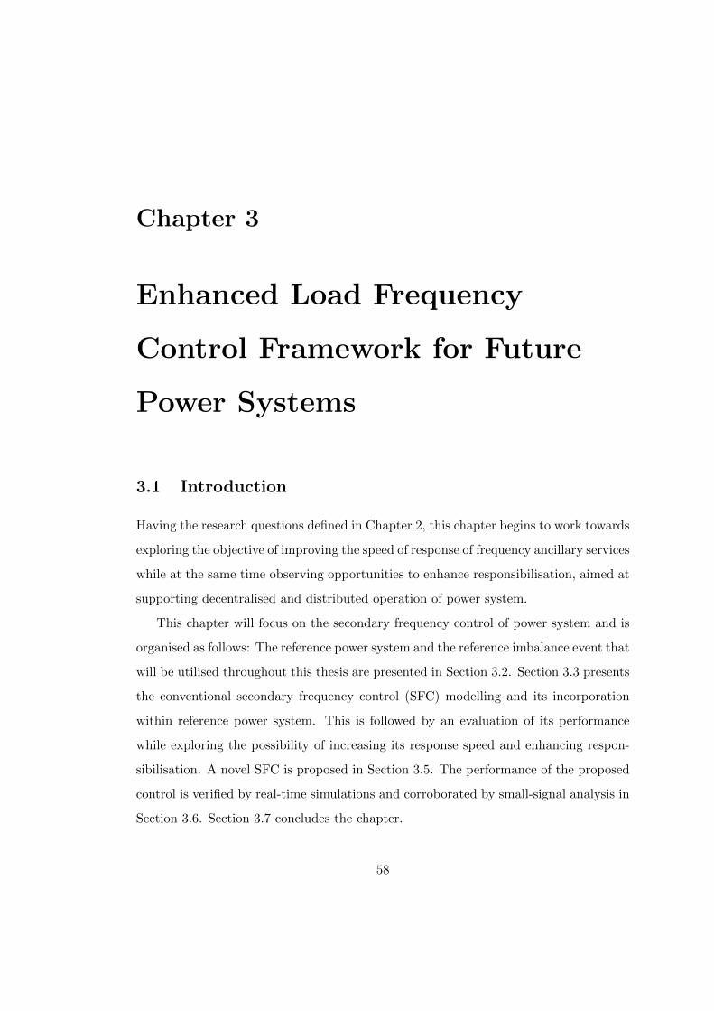
Chapter 3
Enhanced Load Frequency
Control Framework for Future
Power Systems
3.1 Introduction
Having the research questions defined in Chapter 2, this chapter begins to work towards
exploring the objective of improving the speed of response of frequency ancillary services
while at the same time observing opportunities to enhance responsibilisation, aimed at
supporting decentralised and distributed operation of power system.
This chapter will focus on the secondary frequency control of power system and is
organised as follows: The reference power system and the reference imbalance event that
will be utilised throughout this thesis are presented in Section 3.2. Section 3.3 presents
the conventional secondary frequency control (SFC) modelling and its incorporation
within reference power system. This is followed by an evaluation of its performance
while exploring the possibility of increasing its response speed and enhancing respon-
sibilisation. A novel SFC is proposed in Section 3.5. The performance of the proposed
control is verified by real-time simulations and corroborated by small-signal analysis in
Section 3.6. Section 3.7 concludes the chapter.
58
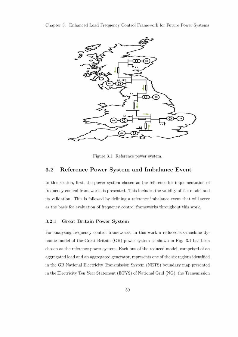
Chapter 3. Enhanced Load Frequency Control Framework for Future Power Systems
5
G1
G2
G3
G6
G5G4
L1
L2
L3
L4
L6
L5
Figure 3.1: Reference power system.
3.2 Reference Power System and Imbalance Event
In this section, first, the power system chosen as the reference for implementation of
frequency control frameworks is presented. This includes the validity of the model and
its validation. This is followed by defining a reference imbalance event that will serve
as the basis for evaluation of frequency control frameworks throughout this work.
3.2.1 Great Britain Power System
For analysing frequency control frameworks, in this work a reduced six-machine dy-
namic model of the Great Britain (GB) power system as shown in Fig. 3.1 has been
chosen as the reference power system. Each bus of the reduced model, comprised of an
aggregated load and an aggregated generator, represents one of the six regions identified
in the GB National Electricity Transmission System (NETS) boundary map presented
in the Electricity Ten Year Statement (ETYS) of National Grid (NG), the Transmission
59
Chapter 3. Enhanced Load Frequency Control Framework for Future Power Systems
System Operator (TSO) of GB [1]. The six regions have been identified around major
generation sources, power flow corridors and load centres [1].
Model Validity
From the discussion presented in Chapter 2, it is clear that the GB grid is inevitably
moving towards a drastic change over the next decade. Considering these changes, the
GB grid offers to be a suitable test bed due to the following:
• The future GB network will encompass all the major challenges expected within
power networks across the world in the coming decades- to name a few, the un-
certainty of secure operation with increasing penetration of intermittent sources
of energy, reducing system inertia and increasing profile of demand side partici-
pation. Interestingly, some of these challenges have begun to present themselves
within the present day GB network.
• As the GB grid has primarily been operated in a centralised manner, with no ele-
ments of decentralised operation as inherent within the larger synchronous grid of
Continental Europe (although limited), the advantages of more decentralised and
distributed operation are expected to be more perceptible and apparent within
the GB grid.
Therefore, the implementation of decentralised/distributed frequency control frame-
works within the GB grid and assessment of its performance, does not only form a basis
for this work but also holds the potential to offer interesting insights to the wider com-
munity including the system operators of GB.
Model Validation
The six-machine model has been developed in RSCAD and simulated in real-time using
a Real Time Digital Simulator from RTDS Technologies, with each area comprising an
aggregated generator and an aggregated load. Each aggregated generator is modelled
as a large synchronous machine connected to the transmission system via a step-up
60
Chapter 3. Enhanced Load Frequency Control Framework for Future Power Systems
transformer (13.8/400kV). The rating of each generator is set according to the pre-
dicted GB 2017 load flow [1]. Each generator is controlled by the widely used IEEE
type 1 static excitation system. A gas turbine and speed governor control the speed
and input torque of each machine. The synchronous machine, excitation system and
gas turbine parameters have been obtained from [2], while the governor speed control
parameters are tuned against real recorded events as will be explained in the following
paragraph. The transmission lines are modelled using Pi-sections with lumped resis-
tance, capacitance, and inductance parameters calculated from the power flow data
provided by the NG ETYS for 2017 [1] as per the methodology presented in [3].
The model has been validated by means of two tests in [4] :
1. Load flow analysis: This test is to evaluate the steady-state performance of the
model. The load flow simulation data of the six-machine test system closely
matches (average error < 3.24%, maximum error < 8.69%) the predicted data
obtained from ETYS, for the winter peak of 2017 [1]. This includes the generation
and demand data at each region and the power flow across the boundaries of the
regions.
2. Dynamic frequency response evaluation: The dynamic response of the six-machine
reference power system model is benchmarked against a number of real historic
frequency deviation events data recorded by phasor measurement units (PMU)
located at various points of the GB power transmission network. In [4], the
event chosen was the trip of the England-France HVDC inter-connector on 11th
of January 2016 leading to a power loss of 900MW. In other words, the model
represents the real-world GB network on the 11th of January, 2016. The total
generation and demand of the model is adjusted to match the values on the day
of the event (total demand=59.56GW). The inertia constant, the governor time
constant, the droop percentage, and the load reference set-point parameters are
tuned to ensure the model frequency response matches the frequency response
(pre-disturbance, rate of change of frequency and frequency nadir) obtained from
the PMUs.
61
Chapter 3. Enhanced Load Frequency Control Framework for Future Power Systems
The model parameters can be found in [4], and in Appendix A of the thesis.
Model Adaptation
The model initial frequency in [4] was adjusted to match that of the real GB power
network on the 11th of January 2016. However, as this work analyses frequency control
frameworks including primary and secondary control, the load reference of the model
was modified such that in steady state the model frequency is 50 Hz.
3.2.2 Reference Imbalance Event- Frequency Disturbance
In this sub-section, the frequency disturbance against which the performance of fre-
quency control frameworks will be assessed is quantified. In addition, justification for
the size of the disturbance is presented, considering the power system of 2030+.
Frequency control should cover the single biggest credible net generation loss (N-1
criteria) that ensures restoration of frequency within acceptable limits should the loss
occur. The biggest credible generation in the GB grid is 1800MW, up from 1320MW
in 2014. As per ENTSO-E guidelines, performance of any frequency control should
be assessed for net generation loss of 1000MW or greater [5]. For the present day
power system, where large synchronous generation still dominate the generation mix,
the assessment of performance of any frequency control against a net generation loss
of 1000 MW is credible. The question that arises is whether this magnitude of dis-
turbance remains to be credible for a 2030+ power system. The remainder of this
sub-section, presents a discussion on the security of supply of the GB grid with respect
to wind energy penetration and HVDC inter-connectors, establishing the credibility of
the magnitude of imbalance event.
Security of supply with high penetration of wind energy: With the decom-
missioning of Longannet power station (capacity 2400MW) in 2016, the commitment of
GB to end the era of reliance on fossil fuel based generation units has been reaffirmed,
with plans to decommission the last coal fired power plant in 2025. Moving forward,
large penetration of smaller sized distributed generation are set to take over the gener-
62
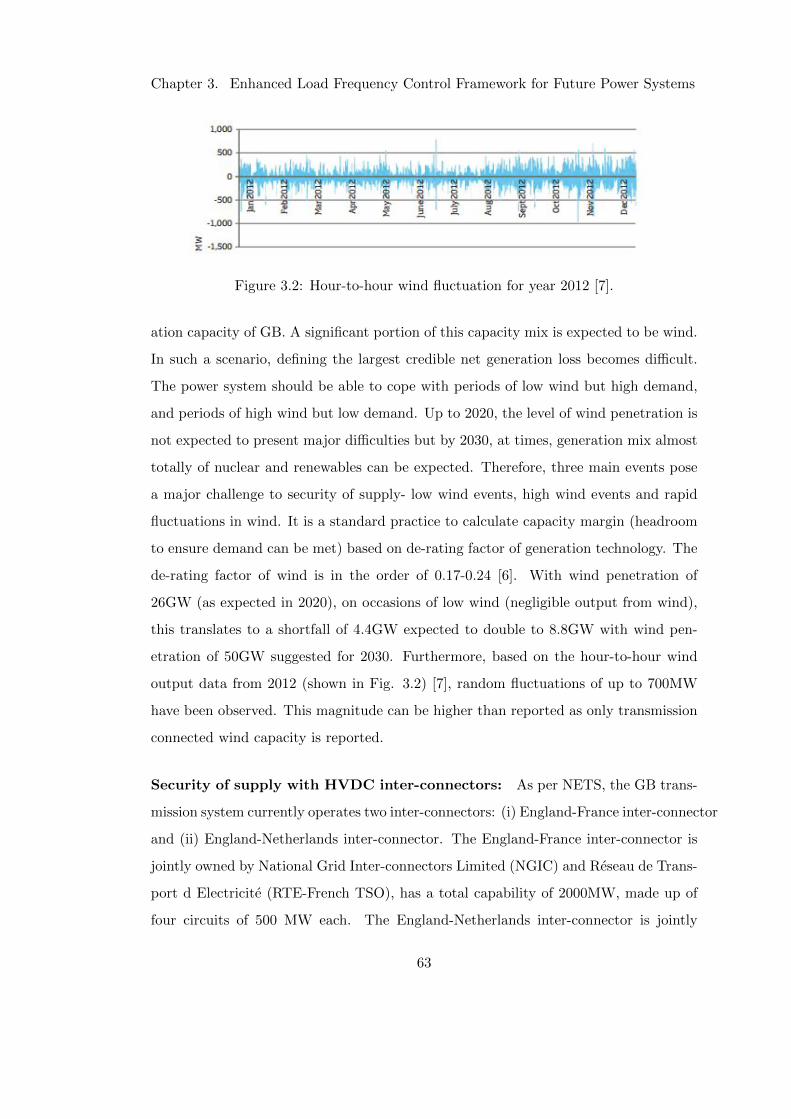
Chapter 3. Enhanced Load Frequency Control Framework for Future Power Systems
Figure 3.2: Hour-to-hour wind fluctuation for year 2012 [7].
ation capacity of GB. A significant portion of this capacity mix is expected to be wind.
In such a scenario, defining the largest credible net generation loss becomes difficult.
The power system should be able to cope with periods of low wind but high demand,
and periods of high wind but low demand. Up to 2020, the level of wind penetration is
not expected to present major difficulties but by 2030, at times, generation mix almost
totally of nuclear and renewables can be expected. Therefore, three main events pose
a major challenge to security of supply- low wind events, high wind events and rapid
fluctuations in wind. It is a standard practice to calculate capacity margin (headroom
to ensure demand can be met) based on de-rating factor of generation technology. The
de-rating factor of wind is in the order of 0.17-0.24 [6]. With wind penetration of
26GW (as expected in 2020), on occasions of low wind (negligible output from wind),
this translates to a shortfall of 4.4GW expected to double to 8.8GW with wind pen-
etration of 50GW suggested for 2030. Furthermore, based on the hour-to-hour wind
output data from 2012 (shown in Fig. 3.2) [7], random fluctuations of up to 700MW
have been observed. This magnitude can be higher than reported as only transmission
connected wind capacity is reported.
Security of supply with HVDC inter-connectors: As per NETS, the GB trans-
mission system currently operates two inter-connectors: (i) England-France inter-connector
and (ii) England-Netherlands inter-connector. The England-France inter-connector is
jointly owned by National Grid Inter-connectors Limited (NGIC) and Reseau de Trans-
port d Electricite (RTE-French TSO), has a total capability of 2000MW, made up of
four circuits of 500 MW each. The England-Netherlands inter-connector is jointly
63
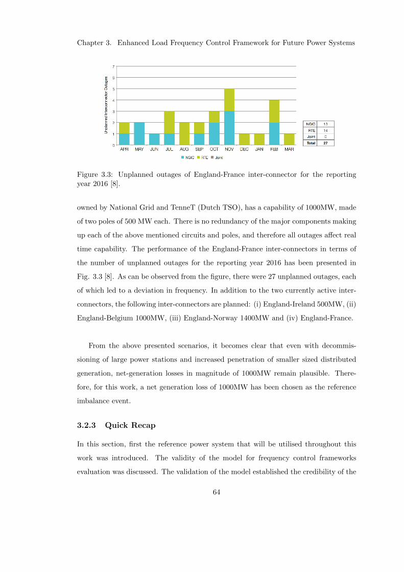
Chapter 3. Enhanced Load Frequency Control Framework for Future Power Systems
Figure 3.3: Unplanned outages of England-France inter-connector for the reportingyear 2016 [8].
owned by National Grid and TenneT (Dutch TSO), has a capability of 1000MW, made
of two poles of 500 MW each. There is no redundancy of the major components making
up each of the above mentioned circuits and poles, and therefore all outages affect real
time capability. The performance of the England-France inter-connectors in terms of
the number of unplanned outages for the reporting year 2016 has been presented in
Fig. 3.3 [8]. As can be observed from the figure, there were 27 unplanned outages, each
of which led to a deviation in frequency. In addition to the two currently active inter-
connectors, the following inter-connectors are planned: (i) England-Ireland 500MW, (ii)
England-Belgium 1000MW, (iii) England-Norway 1400MW and (iv) England-France.
From the above presented scenarios, it becomes clear that even with decommis-
sioning of large power stations and increased penetration of smaller sized distributed
generation, net-generation losses in magnitude of 1000MW remain plausible. There-
fore, for this work, a net generation loss of 1000MW has been chosen as the reference
imbalance event.
3.2.3 Quick Recap
In this section, first the reference power system that will be utilised throughout this
work was introduced. The validity of the model for frequency control frameworks
evaluation was discussed. The validation of the model established the credibility of the
64

Chapter 3. Enhanced Load Frequency Control Framework for Future Power Systems
LPmiP
Primary Control LoopSecondary Control Loop (AGC)
f
+
iACE
Ip
KK
s
1,
M
ij
j j i
T
2 s
iB
giP1
2 i iH s D
1 iR
1
1giT s
1
1
ai
bi
T s
T s
+
DSM Aggregators
ciP
1,
M
ij j
j j i
T f
EVAggregator 1
...
ESSDSA
EVAggregator M
ESS
CG
DSA
iP DSA
iP
tie
iPtie
iP
Area i
Interconnection with other areas
J=1...M, J≠i
Figure 3.4: Load Frequency Control Framework.
developed model. Furthermore, the magnitude of the imbalance event was quantified
and justified.
3.3 Legacy Load Frequency Control Framework
A synchronous power system is divided into a number of LFC areas, each responsible to
maintain the frequency of the system by means of maintaining its own scheduled power
flows. The frequency is restored to its nominal value by means of changing the set-point
of certain conventional generators (CG) chosen to participate in the restoration process
[5], [9].
3.3.1 Conventional LFC Framework Modeling
Consider an interconnected power system withM control areas indexed by i = 1, · · · ,M .
The LFC model of the ith control area is presented in Fig. 3.4. As shown, the LFC
comprises a primary control loop and a secondary control loop, where the aim of pri-
mary control is to contain the frequency deviation caused by power imbalance in any
control area, while the secondary control, i.e. automatic generation control (AGC), is
responsible to recover the frequency back to its nominal value [5]. The system dynamics
of the ith area can be represented by the following differential equations
(3.1)∆fi (t) = − D
2H∆fi (t) +
1
2Hi(∆Pmi (t)−∆PL,i (t))−∆Ptie,i (t) + ∆PDSA,i (t))
65
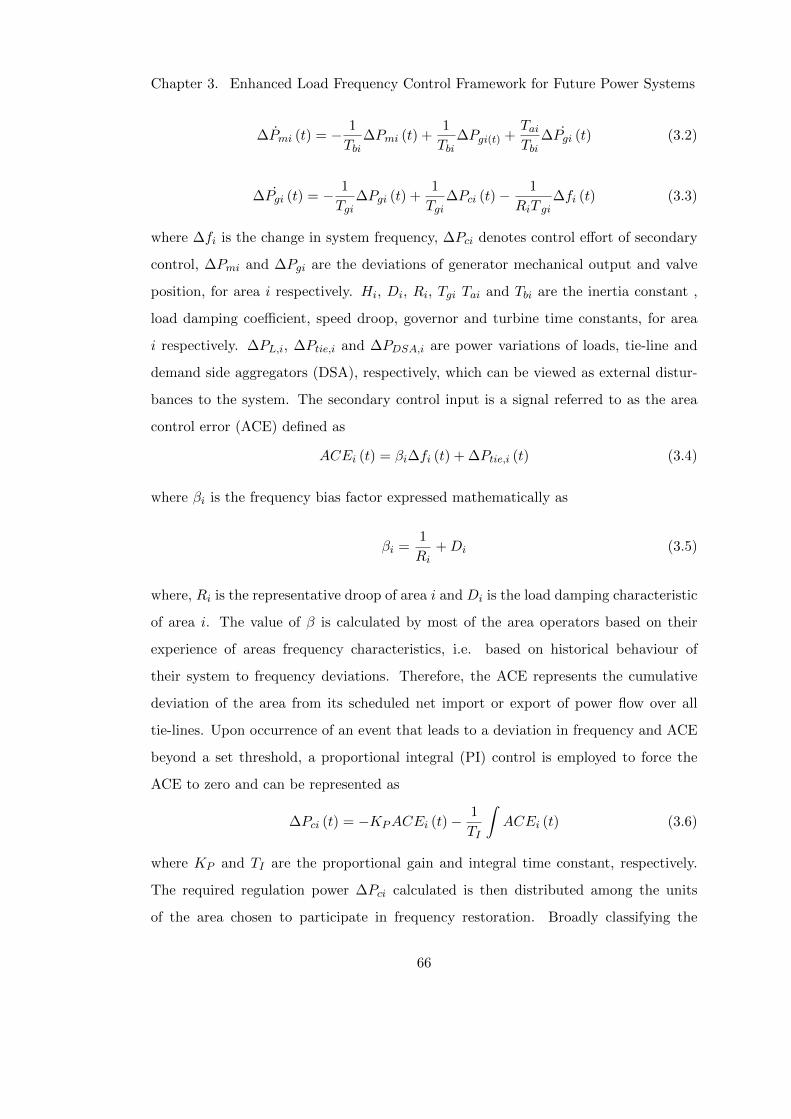
Chapter 3. Enhanced Load Frequency Control Framework for Future Power Systems
(3.2)∆Pmi (t) = − 1
Tbi∆Pmi (t) +
1
Tbi∆Pgi(t) +
TaiTbi
∆Pgi (t)
(3.3)∆Pgi (t) = − 1
Tgi∆Pgi (t) +
1
Tgi∆Pci (t)− 1
RiT gi∆fi (t)
where ∆fi is the change in system frequency, ∆Pci denotes control effort of secondary
control, ∆Pmi and ∆Pgi are the deviations of generator mechanical output and valve
position, for area i respectively. Hi, Di, Ri, Tgi Tai and Tbi are the inertia constant ,
load damping coefficient, speed droop, governor and turbine time constants, for area
i respectively. ∆PL,i, ∆Ptie,i and ∆PDSA,i are power variations of loads, tie-line and
demand side aggregators (DSA), respectively, which can be viewed as external distur-
bances to the system. The secondary control input is a signal referred to as the area
control error (ACE) defined as
(3.4)ACEi (t) = βi∆fi (t) + ∆Ptie,i (t)
where βi is the frequency bias factor expressed mathematically as
βi =1
Ri+Di (3.5)
where, Ri is the representative droop of area i and Di is the load damping characteristic
of area i. The value of β is calculated by most of the area operators based on their
experience of areas frequency characteristics, i.e. based on historical behaviour of
their system to frequency deviations. Therefore, the ACE represents the cumulative
deviation of the area from its scheduled net import or export of power flow over all
tie-lines. Upon occurrence of an event that leads to a deviation in frequency and ACE
beyond a set threshold, a proportional integral (PI) control is employed to force the
ACE to zero and can be represented as
(3.6)∆Pci (t) = −KPACEi (t)− 1
TI
∫ACEi (t)
where KP and TI are the proportional gain and integral time constant, respectively.
The required regulation power ∆Pci calculated is then distributed among the units
of the area chosen to participate in frequency restoration. Broadly classifying the
66
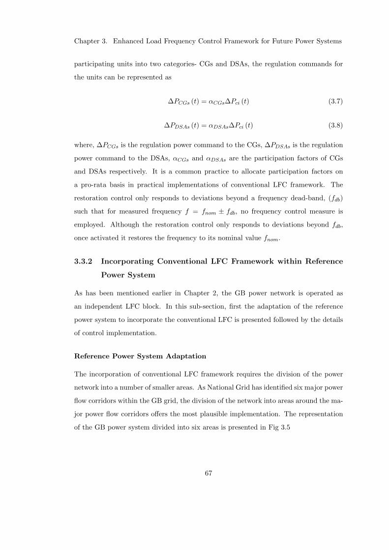
Chapter 3. Enhanced Load Frequency Control Framework for Future Power Systems
participating units into two categories- CGs and DSAs, the regulation commands for
the units can be represented as
∆PCGs (t) = αCGs∆Pci (t) (3.7)
∆PDSAs (t) = αDSAs∆Pci (t) (3.8)
where, ∆PCGs is the regulation power command to the CGs, ∆PDSAs is the regulation
power command to the DSAs, αCGs and αDSAs are the participation factors of CGs
and DSAs respectively. It is a common practice to allocate participation factors on
a pro-rata basis in practical implementations of conventional LFC framework. The
restoration control only responds to deviations beyond a frequency dead-band, (fdb)
such that for measured frequency f = fnom ± fdb, no frequency control measure is
employed. Although the restoration control only responds to deviations beyond fdb,
once activated it restores the frequency to its nominal value fnom.
3.3.2 Incorporating Conventional LFC Framework within Reference
Power System
As has been mentioned earlier in Chapter 2, the GB power network is operated as
an independent LFC block. In this sub-section, first the adaptation of the reference
power system to incorporate the conventional LFC is presented followed by the details
of control implementation.
Reference Power System Adaptation
The incorporation of conventional LFC framework requires the division of the power
network into a number of smaller areas. As National Grid has identified six major power
flow corridors within the GB grid, the division of the network into areas around the ma-
jor power flow corridors offers the most plausible implementation. The representation
of the GB power system divided into six areas is presented in Fig 3.5
67
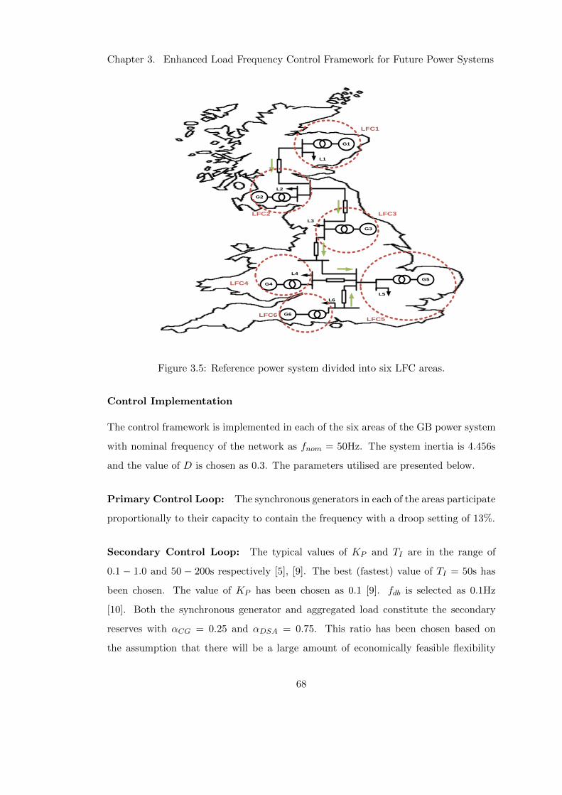
Chapter 3. Enhanced Load Frequency Control Framework for Future Power Systems
5
G1
G2
G3
G6
G5G4
L1
L2
L3
L4
L6
L5
LFC1
LFC2 LFC3
LFC4
LFC5LFC6
Figure 3.5: Reference power system divided into six LFC areas.
Control Implementation
The control framework is implemented in each of the six areas of the GB power system
with nominal frequency of the network as fnom = 50Hz. The system inertia is 4.456s
and the value of D is chosen as 0.3. The parameters utilised are presented below.
Primary Control Loop: The synchronous generators in each of the areas participate
proportionally to their capacity to contain the frequency with a droop setting of 13%.
Secondary Control Loop: The typical values of KP and TI are in the range of
0.1 − 1.0 and 50 − 200s respectively [5], [9]. The best (fastest) value of TI = 50s has
been chosen. The value of KP has been chosen as 0.1 [9]. fdb is selected as 0.1Hz
[10]. Both the synchronous generator and aggregated load constitute the secondary
reserves with αCG = 0.25 and αDSA = 0.75. This ratio has been chosen based on
the assumption that there will be a large amount of economically feasible flexibility
68
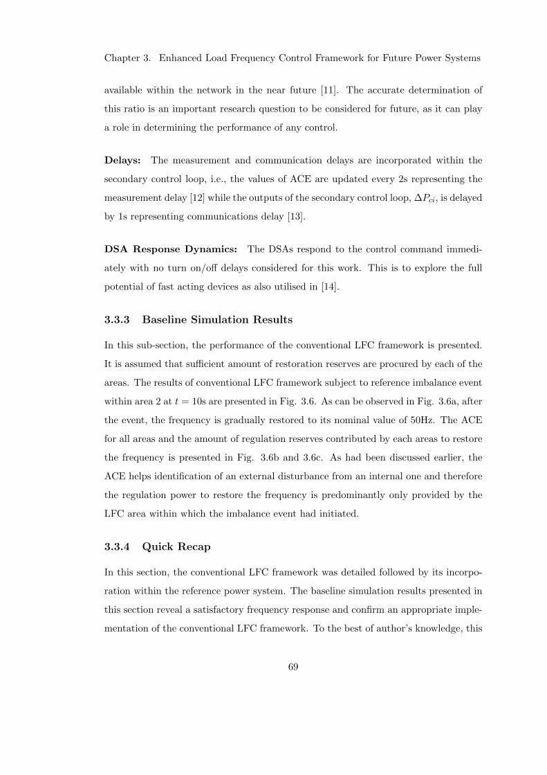
Chapter 3. Enhanced Load Frequency Control Framework for Future Power Systems
available within the network in the near future [11]. The accurate determination of
this ratio is an important research question to be considered for future, as it can play
a role in determining the performance of any control.
Delays: The measurement and communication delays are incorporated within the
secondary control loop, i.e., the values of ACE are updated every 2s representing the
measurement delay [12] while the outputs of the secondary control loop, ∆Pci, is delayed
by 1s representing communications delay [13].
DSA Response Dynamics: The DSAs respond to the control command immedi-
ately with no turn on/off delays considered for this work. This is to explore the full
potential of fast acting devices as also utilised in [14].
3.3.3 Baseline Simulation Results
In this sub-section, the performance of the conventional LFC framework is presented.
It is assumed that sufficient amount of restoration reserves are procured by each of the
areas. The results of conventional LFC framework subject to reference imbalance event
within area 2 at t = 10s are presented in Fig. 3.6. As can be observed in Fig. 3.6a, after
the event, the frequency is gradually restored to its nominal value of 50Hz. The ACE
for all areas and the amount of regulation reserves contributed by each areas to restore
the frequency is presented in Fig. 3.6b and 3.6c. As had been discussed earlier, the
ACE helps identification of an external disturbance from an internal one and therefore
the regulation power to restore the frequency is predominantly only provided by the
LFC area within which the imbalance event had initiated.
3.3.4 Quick Recap
In this section, the conventional LFC framework was detailed followed by its incorpo-
ration within the reference power system. The baseline simulation results presented in
this section reveal a satisfactory frequency response and confirm an appropriate imple-
mentation of the conventional LFC framework. To the best of author’s knowledge, this
69
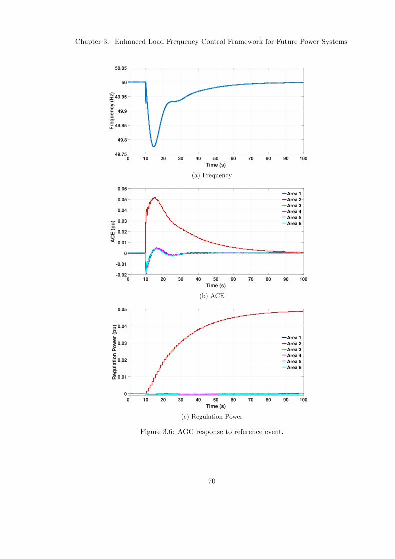
Chapter 3. Enhanced Load Frequency Control Framework for Future Power Systems
0 10 20 30 40 50 60 70 80 90 100
Time (s)
49.75
49.8
49.85
49.9
49.95
50
50.05
Fre
qu
en
cy
(H
z)
(a) Frequency
0 10 20 30 40 50 60 70 80 90 100
Time (s)
-0.02
-0.01
0
0.01
0.02
0.03
0.04
0.05
0.06
AC
E (
pu
)
Area 1
Area 2
Area 3
Area 4
Area 5
Area 6
(b) ACE
0 10 20 30 40 50 60 70 80 90 100
Time (s)
0
0.01
0.02
0.03
0.04
0.05
Re
gu
lati
on
Po
we
r (p
u)
Area 1
Area 2
Area 3
Area 4
Area 5
Area 6
(c) Regulation Power
Figure 3.6: AGC response to reference event.
70
Chapter 3. Enhanced Load Frequency Control Framework for Future Power Systems
0 50 100 150 200 250 300
Time (s)
49.8
49.9
50F
req
ue
nc
y (
Hz)
TI= 50s
TI= 100s
TI= 150s
TI= 200s
Figure 3.7: System frequency response subject to reference imbalance event in Area 2for different values of TI .
is the first implementation where the conventional LFC framework has been incorpo-
rated within the GB grid. The incorporation of conventional LFC framework within
the GB grid begins to introduce a degree of decentralisation and responsibilisation.
Remedial measures are taken closer to the location of the imbalance event, i.e. within
the area of the disturbance as opposed to the current practice within GB grid where
the response is from across GB.
3.4 Analysis of Conventional LFC Framework
Having incorporated the conventional LFC framework within the reference power sys-
tem and establishing a baseline response, in this section, the performance of the con-
ventional framework is analysed. The analysis takes into consideration the changes
expected within the near future, aimed at identifying issues that might need to be
addressed or areas where the performance of the conventional LFC can be further
improved.
For the baseline simulation results presented in Section 3.3.3, although 75% of the
regulation power is from DSAs (based on the participation factor chosen) that utilize
fast acting demand side resources with no turn on/off delays, the effect of their fast
71
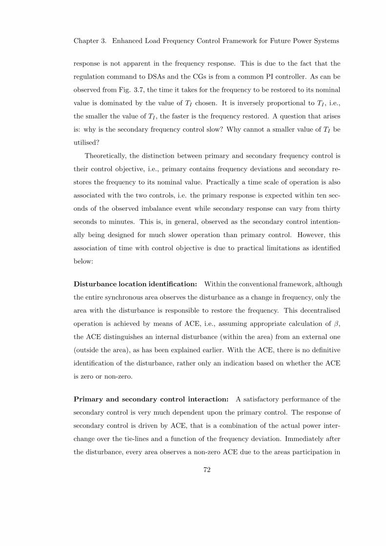
Chapter 3. Enhanced Load Frequency Control Framework for Future Power Systems
response is not apparent in the frequency response. This is due to the fact that the
regulation command to DSAs and the CGs is from a common PI controller. As can be
observed from Fig. 3.7, the time it takes for the frequency to be restored to its nominal
value is dominated by the value of TI chosen. It is inversely proportional to TI , i.e.,
the smaller the value of TI , the faster is the frequency restored. A question that arises
is: why is the secondary frequency control slow? Why cannot a smaller value of TI be
utilised?
Theoretically, the distinction between primary and secondary frequency control is
their control objective, i.e., primary contains frequency deviations and secondary re-
stores the frequency to its nominal value. Practically a time scale of operation is also
associated with the two controls, i.e. the primary response is expected within ten sec-
onds of the observed imbalance event while secondary response can vary from thirty
seconds to minutes. This is, in general, observed as the secondary control intention-
ally being designed for much slower operation than primary control. However, this
association of time with control objective is due to practical limitations as identified
below:
Disturbance location identification: Within the conventional framework, although
the entire synchronous area observes the disturbance as a change in frequency, only the
area with the disturbance is responsible to restore the frequency. This decentralised
operation is achieved by means of ACE, i.e., assuming appropriate calculation of β,
the ACE distinguishes an internal disturbance (within the area) from an external one
(outside the area), as has been explained earlier. With the ACE, there is no definitive
identification of the disturbance, rather only an indication based on whether the ACE
is zero or non-zero.
Primary and secondary control interaction: A satisfactory performance of the
secondary control is very much dependent upon the primary control. The response of
secondary control is driven by ACE, that is a combination of the actual power inter-
change over the tie-lines and a function of the frequency deviation. Immediately after
the disturbance, every area observes a non-zero ACE due to the areas participation in
72
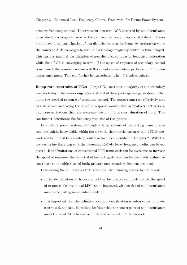
Chapter 3. Enhanced Load Frequency Control Framework for Future Power Systems
primary frequency control. This transient non-zero ACE observed by non-disturbance
areas slowly converges to zero as the primary frequency response stabilizes. There-
fore, to avoid the participation of non disturbance areas in frequency restoration while
the transient ACE converges to zero, the secondary frequency control is time delayed.
This ensures minimal participation of non disturbance areas in frequency restoration
while their ACE is converging to zero. If the speed of response of secondary control
is increased, the transient non-zero ACE can enforce secondary participation from non
disturbance areas. This can further be exacerbated when β is miscalculated.
Ramp-rate constraint of CGs: Large CGs constitute a majority of the secondary
reserves today. The power ramp rate constraint of these participating generators further
limits the speed of response of secondary control. The power ramp-rate effectively acts
as a delay and increasing the speed of response would cause sympathetic activations,
i.e., more activations than are necessary but only for a short duration of time. This
can further deteriorate the frequency response of the system.
In a future power system, although a large volume of fast acting demand side
resources might be available within the network, their participation within LFC frame-
work will be limited to secondary control as had been identified in Chapter 2. With the
decreasing inertia, along with the increasing RoCoF, lower frequency nadirs can be ex-
pected. If the limitations of conventional LFC framework can be overcome to increase
the speed of response, the potential of fast acting devices can be effectively utilised to
contribute to the objectives of both, primary and secondary frequency control.
Considering the limitations identified above, the following can be hypothesised:
• If the identification of the location of the disturbance can be definitive, the speed
of response of conventional LFC can be improved, with no risk of non-disturbance
area participating in secondary control.
• It is important that the definitive location identification is autonomous, fully de-
centralised, and fast. It needs to be faster than the convergence of non-disturbance
areas transient ACE to zero as in the conventional LFC framework.
73
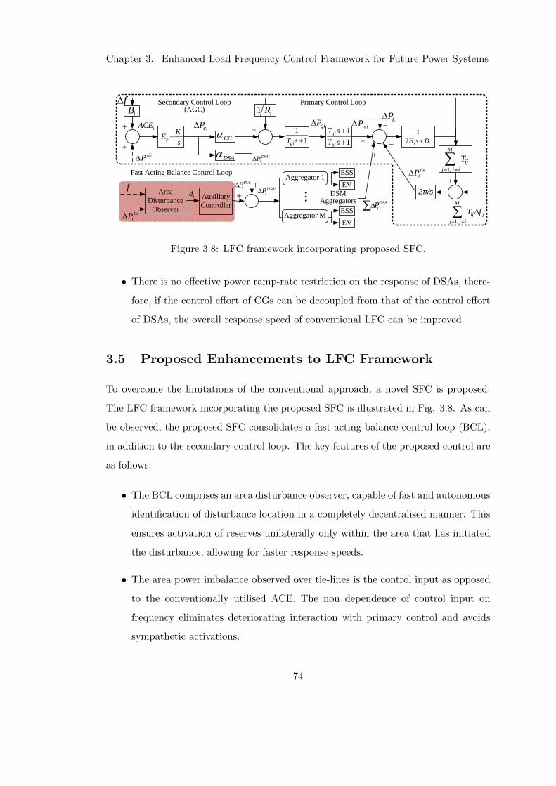
Chapter 3. Enhanced Load Frequency Control Framework for Future Power Systems
LPmiP
Primary Control LoopSecondary Control Loop (AGC)
f
+
iACE
Ip
KK
s
1,
M
ij
j j i
T
iB
giP1
2 i iH s D
1 iR
1
1giT s
1
1
ai
bi
T s
T s
+
DSM Aggregators
ciP
1,
M
ij j
j j i
T f
EVAggregator 1
...
ESS
DSA
EVAggregator M
ESS
CG
DSA
iP
Area
Disturbance
Observer
Auxiliary
Controller
Fast Acting Balance Control Loop
f *DSA
iP
BCL
iP
id
DSA
iP
tie
iP
tie
iP
tie
iP
2π/s
Figure 3.8: LFC framework incorporating proposed SFC.
• There is no effective power ramp-rate restriction on the response of DSAs, there-
fore, if the control effort of CGs can be decoupled from that of the control effort
of DSAs, the overall response speed of conventional LFC can be improved.
3.5 Proposed Enhancements to LFC Framework
To overcome the limitations of the conventional approach, a novel SFC is proposed.
The LFC framework incorporating the proposed SFC is illustrated in Fig. 3.8. As can
be observed, the proposed SFC consolidates a fast acting balance control loop (BCL),
in addition to the secondary control loop. The key features of the proposed control are
as follows:
• The BCL comprises an area disturbance observer, capable of fast and autonomous
identification of disturbance location in a completely decentralised manner. This
ensures activation of reserves unilaterally only within the area that has initiated
the disturbance, allowing for faster response speeds.
• The area power imbalance observed over tie-lines is the control input as opposed
to the conventionally utilised ACE. The non dependence of control input on
frequency eliminates deteriorating interaction with primary control and avoids
sympathetic activations.
74
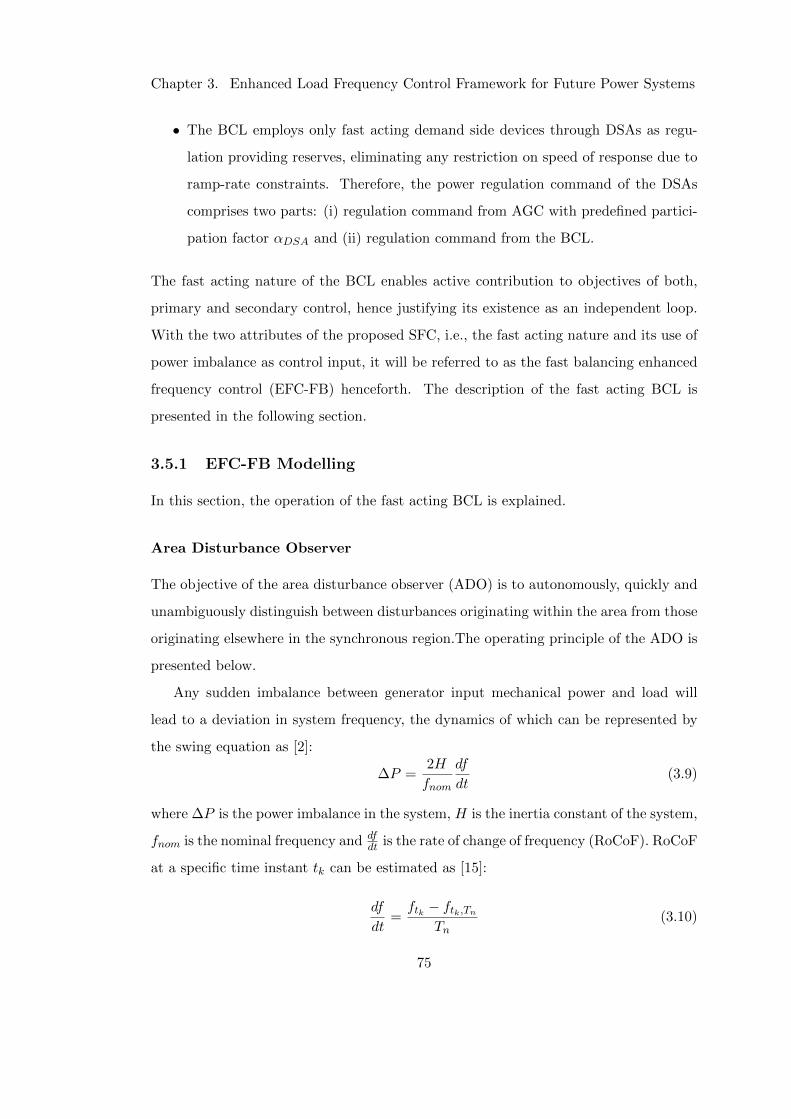
Chapter 3. Enhanced Load Frequency Control Framework for Future Power Systems
• The BCL employs only fast acting demand side devices through DSAs as regu-
lation providing reserves, eliminating any restriction on speed of response due to
ramp-rate constraints. Therefore, the power regulation command of the DSAs
comprises two parts: (i) regulation command from AGC with predefined partici-
pation factor αDSA and (ii) regulation command from the BCL.
The fast acting nature of the BCL enables active contribution to objectives of both,
primary and secondary control, hence justifying its existence as an independent loop.
With the two attributes of the proposed SFC, i.e., the fast acting nature and its use of
power imbalance as control input, it will be referred to as the fast balancing enhanced
frequency control (EFC-FB) henceforth. The description of the fast acting BCL is
presented in the following section.
3.5.1 EFC-FB Modelling
In this section, the operation of the fast acting BCL is explained.
Area Disturbance Observer
The objective of the area disturbance observer (ADO) is to autonomously, quickly and
unambiguously distinguish between disturbances originating within the area from those
originating elsewhere in the synchronous region.The operating principle of the ADO is
presented below.
Any sudden imbalance between generator input mechanical power and load will
lead to a deviation in system frequency, the dynamics of which can be represented by
the swing equation as [2]:
∆P =2H
fnom
df
dt(3.9)
where ∆P is the power imbalance in the system, H is the inertia constant of the system,
fnom is the nominal frequency and dfdt is the rate of change of frequency (RoCoF). RoCoF
at a specific time instant tk can be estimated as [15]:
df
dt=ftk − ftk,Tn
Tn(3.10)
75
Chapter 3. Enhanced Load Frequency Control Framework for Future Power Systems
where Tn is the length of the measuring window.Within a synchronous area A and for
area under consideration i, the neighborhood can be defined as NHi = {i,AN i} ⊆ A.
With j ∈ AN i as adjacent areas coupled over tie-lines with breaker state δij , the change
in tie-line power flow for area i, subject to the imbalance, can be calculated as
(3.11)∆P tiei =∑
j∈AN i
δijPtie0,i −
∑j∈AN i
δijPtiemeas,i
where P tie0,i and P tiemeas,i are the scheduled and measured tie-line power flow respectively.
As the change in electric power flow is immediate, upon occurrence of an imbalance
such that ∆P tiei ≥ ∆P tieTh,i, measuring the extremum of dfdt as df
dt
∗, for ∆P tiei , dfdt
∗ 6= 0,
the disturbance is classified as originating within the area if
floor
dfdt
∗∣∣∣dfdt ∗∣∣∣+ 1
− floor
−dfdt
∗∣∣∣dfdt ∗∣∣∣+ 1
6= floor
(∆P tiei∣∣∆P tiei ∣∣+ 1
)− floor
(−∆P tiei∣∣∆P tiei ∣∣+ 1
)(3.12)
where floor represents the flooring function, ∆P tieTh,i is the threshold of change in tie-line
power flow set based on largest expected load variation in area i. Upon satisfying equa-
tion (3.12), the output of the disturbance observer is di =∆P tiei , else di = 0. Therefore,
each area of A can identify disturbances originating within themselves based on local
measurements in a decentralised manner within 200ms. Although the identification is
fast, there might be a frequency dead-band, (fdb) such that for measured frequency
f = fnom ± fdb, no frequency control measure is employed.
Auxiliary Controller
The output of ADO is an input to the auxiliary controller, and for when equation (3.12)
is true, di should be controlled to zero. Employing a PI control, the control effort can
be represented as
∆PBCLi (t) = −KP,auxdi (t)− 1
TI,aux
∫di (t) (3.13)
where Kp,aux and TI,aux are the proportional gain and integral time constant of the
auxiliary control. Contrary to the secondary control loop, where smaller values of TI
76
Chapter 3. Enhanced Load Frequency Control Framework for Future Power Systems
are limited by ramp rate constraints of CGs, TI,aux can be chosen for faster response.
The use of PI control for BCL is not mandatory and the output of ADO can be an
auxiliary hook for direct load frequency control [16]. The effective power regulation
command issued to the DSAs can be represented as
∆PDSA∗
i (t) = ∆PDSAi (t) + ∆PBCLi (t) (3.14)
Low Pass Filtering
To suppress the measurement noise and to smoothen the response of BCL, a low pass
filter is utilised for ∆P tiei and dfdt . The filtered signals at time instant tk can be repre-
sented as
∆P tie,∗i (tk) = (1− a) ∆P tie,∗i (tk − 1) + a∆P tiei (tk) (3.15)
df
dt
∗(tk) = (1− a)
df
dt
∗(tk − 1) + a
df
dt(tk) (3.16)
where a = thTf+th
, with th as the time step of control implementation and Tf as the
filter time constant. It is important to choose filter time constant such that it renders
satisfactory quality of input while attributing least delay.
3.5.2 Incorporating EFC-FB within Reference Power System
The incorporation of the proposed EFC-FB does not require any further adaptation of
the reference power system. The EFC-FB is incorporated within the LFC framework
implemented in each of the six areas of the GB power system similar to the incorporation
of the conventional LFC framework. The parameters of primary control loop and
secondary control loop are same as utilised for conventional LFC framework. The
additional parameters chosen for implementation of the proposed EFC-FB are presented
below.
Balance Control Loop: With aggregated loads participating as reserves, the val-
ues of KP,aux and TI,aux are selected as 0.1 and 5s respectively. With no ramp-rate
constraints, a smaller value of TI,aux has been chosen to demonstrate the effectiveness
77
Chapter 3. Enhanced Load Frequency Control Framework for Future Power Systems
of BCL. For the ADO, the values of ∆P tieTh,i = 50MW, Tn = 0.02s and Tf = 0.02s are
selected.
Delays: The measurement and communication delays are incorporated within the
balance control loop similar to as incorporated within secondary control loop , i.e.,
the values of ACE are updated every 2s representing the measurement delay while the
outputs of the BCL, ∆PBCLi are delayed by 1s representing communications delay.
3.5.3 Quick Recap
In this section, a novel SFC referred to as EFC-FB is introduced and its modelling
presented. The design of EFC-FB overcomes the limitations set upon the conventional
LFC framework, as had been identified in Section 3.4. The incorporation of EFC-FB
within the reference power system with necessary parameters is presented.
3.6 Performance Evaluation
In this section, the applicability of the proposed EFC-FB is validated by means of
real-time simulations.
Methodology: The performance of LFC framework with EFC-FB is compared to
that of conventional LFC framework by means of the following two defined scenarios
1. Response to Reference Imbalance Event: The system is subject to two
disturbances, loss of generation and loss of load.
2. Sensitivity Analysis: A sensitivity analysis by varying the inertia of the system
and the size of disturbance is undertaken.
To aid the assessment, two key indicators are defined as:
• Frequency Restoration Time (TRest): To asses the T rest of the controllers,
an error margin ε = 0.01 is defined such that T rest is the time interval between
the initiation of disturbance to the point when |∆f |= |f − fnom|< ε, and can be
represented as T rest = {T rest ∈ R : ∀ t > T rest, |∆f |≤ ε}.
78
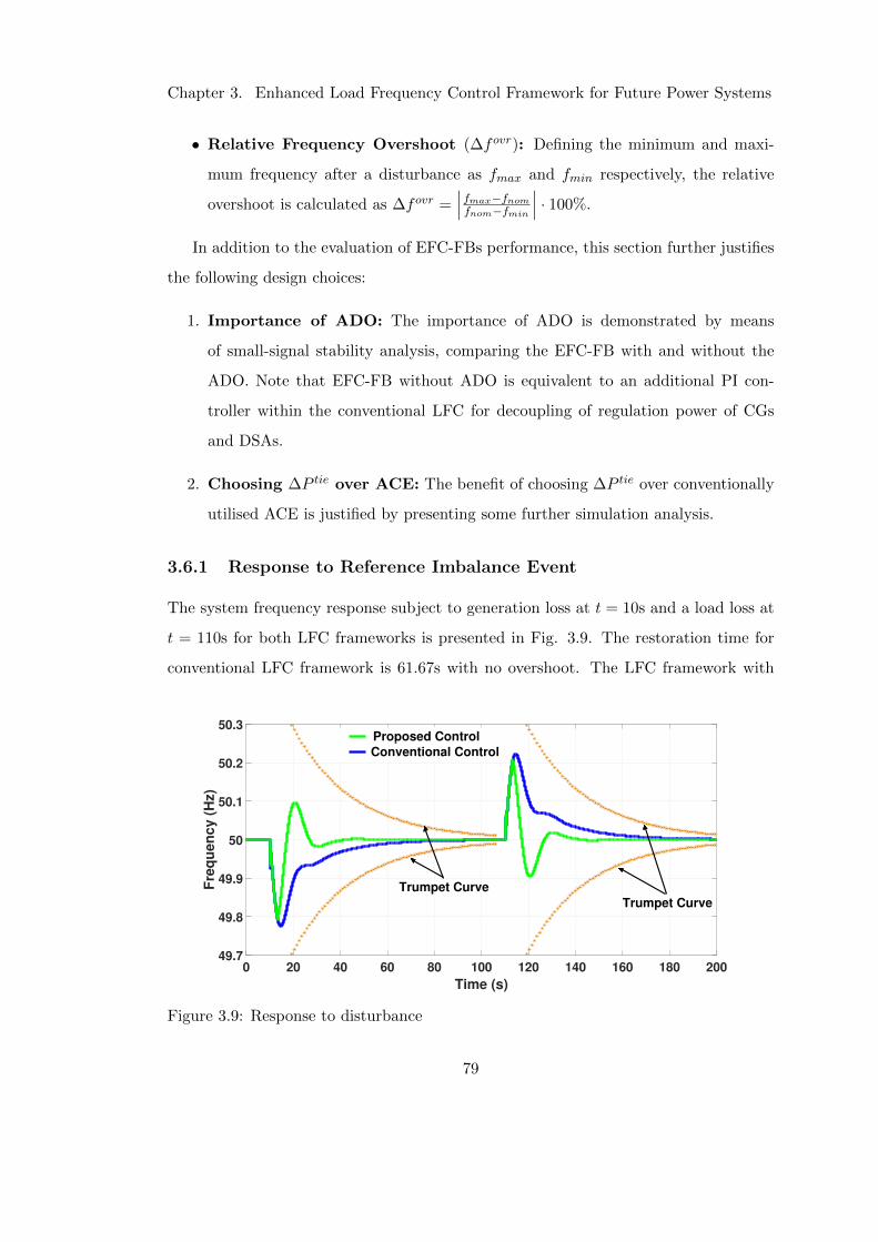
Chapter 3. Enhanced Load Frequency Control Framework for Future Power Systems
• Relative Frequency Overshoot (∆fovr): Defining the minimum and maxi-
mum frequency after a disturbance as fmax and fmin respectively, the relative
overshoot is calculated as ∆fovr =∣∣∣fmax−fnomfnom−fmin
∣∣∣ · 100%.
In addition to the evaluation of EFC-FBs performance, this section further justifies
the following design choices:
1. Importance of ADO: The importance of ADO is demonstrated by means
of small-signal stability analysis, comparing the EFC-FB with and without the
ADO. Note that EFC-FB without ADO is equivalent to an additional PI con-
troller within the conventional LFC for decoupling of regulation power of CGs
and DSAs.
2. Choosing ∆P tie over ACE: The benefit of choosing ∆P tie over conventionally
utilised ACE is justified by presenting some further simulation analysis.
3.6.1 Response to Reference Imbalance Event
The system frequency response subject to generation loss at t = 10s and a load loss at
t = 110s for both LFC frameworks is presented in Fig. 3.9. The restoration time for
conventional LFC framework is 61.67s with no overshoot. The LFC framework with
0 20 40 60 80 100 120 140 160 180 200
Time (s)
49.7
49.8
49.9
50
50.1
50.2
50.3
Fre
qu
en
cy
(H
z)
Trumpet Curve
Trumpet Curve
Proposed Control
Conventional Control
Figure 3.9: Response to disturbance
79
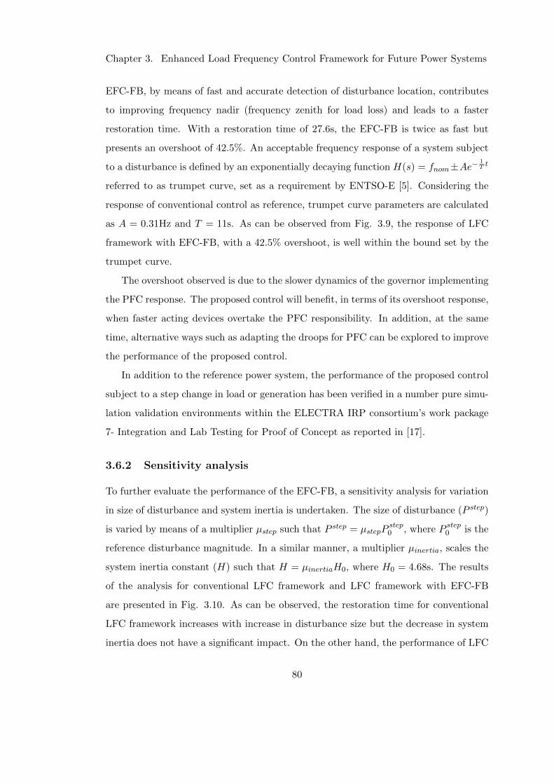
Chapter 3. Enhanced Load Frequency Control Framework for Future Power Systems
EFC-FB, by means of fast and accurate detection of disturbance location, contributes
to improving frequency nadir (frequency zenith for load loss) and leads to a faster
restoration time. With a restoration time of 27.6s, the EFC-FB is twice as fast but
presents an overshoot of 42.5%. An acceptable frequency response of a system subject
to a disturbance is defined by an exponentially decaying function H(s) = fnom±Ae−1Tt
referred to as trumpet curve, set as a requirement by ENTSO-E [5]. Considering the
response of conventional control as reference, trumpet curve parameters are calculated
as A = 0.31Hz and T = 11s. As can be observed from Fig. 3.9, the response of LFC
framework with EFC-FB, with a 42.5% overshoot, is well within the bound set by the
trumpet curve.
The overshoot observed is due to the slower dynamics of the governor implementing
the PFC response. The proposed control will benefit, in terms of its overshoot response,
when faster acting devices overtake the PFC responsibility. In addition, at the same
time, alternative ways such as adapting the droops for PFC can be explored to improve
the performance of the proposed control.
In addition to the reference power system, the performance of the proposed control
subject to a step change in load or generation has been verified in a number pure simu-
lation validation environments within the ELECTRA IRP consortium’s work package
7- Integration and Lab Testing for Proof of Concept as reported in [17].
3.6.2 Sensitivity analysis
To further evaluate the performance of the EFC-FB, a sensitivity analysis for variation
in size of disturbance and system inertia is undertaken. The size of disturbance (P step)
is varied by means of a multiplier µstep such that P step = µstepPstep0 , where P step0 is the
reference disturbance magnitude. In a similar manner, a multiplier µinertia, scales the
system inertia constant (H) such that H = µinertiaH0, where H0 = 4.68s. The results
of the analysis for conventional LFC framework and LFC framework with EFC-FB
are presented in Fig. 3.10. As can be observed, the restoration time for conventional
LFC framework increases with increase in disturbance size but the decrease in system
inertia does not have a significant impact. On the other hand, the performance of LFC
80
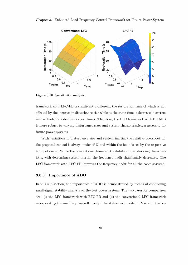
Chapter 3. Enhanced Load Frequency Control Framework for Future Power Systems
µStep
µInertia
701
80
0.9 2
Re
sto
rati
on
Tim
e (
s)
90
Conventional LFC
0.8 1.5
100
0.71
0.6 µStep
µInertia
251
30
0.9 2
Re
sto
rati
on
Tim
e (
s)
35
EFC-FB
0.8 1.5
40
0.71
0.630
40
50
60
70
80
90
100
Figure 3.10: Sensitivity analysis
framework with EFC-FB is significantly different, the restoration time of which is not
effected by the increase in disturbance size while at the same time, a decrease in system
inertia leads to faster restoration times. Therefore, the LFC framework with EFC-FB
is more robust to varying disturbance sizes and system characteristics, a necessity for
future power systems.
With variations in disturbance size and system inertia, the relative overshoot for
the proposed control is always under 45% and within the bounds set by the respective
trumpet curve. While the conventional framework exhibits no overshooting character-
istic, with decreasing system inertia, the frequency nadir significantly decreases. The
LFC framework with EFC-FB improves the frequency nadir for all the cases assessed.
3.6.3 Importance of ADO
In this sub-section, the importance of ADO is demonstrated by means of conducting
small-signal stability analysis on the test power system. The two cases for comparison
are: (i) the LFC framework with EFC-FB and (ii) the conventional LFC framework
incorporating the auxiliary controller only. The state-space model of M-area intercon-
81
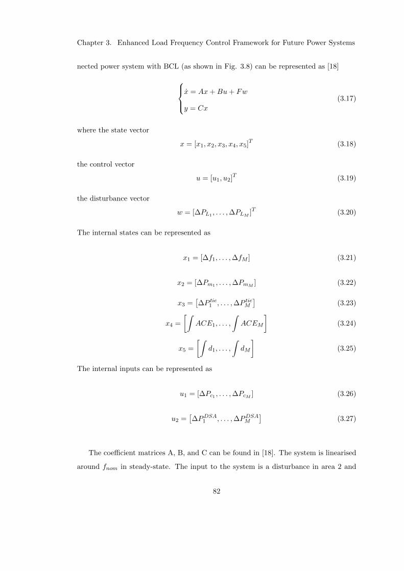
Chapter 3. Enhanced Load Frequency Control Framework for Future Power Systems
nected power system with BCL (as shown in Fig. 3.8) can be represented as [18]
x = Ax+Bu+ Fw
y = Cx
(3.17)
where the state vector
x = [x1, x2, x3, x4, x5]T (3.18)
the control vector
u = [u1, u2]T (3.19)
the disturbance vector
w = [∆PL1 , . . . ,∆PLM ]T (3.20)
The internal states can be represented as
x1 = [∆f1, . . . ,∆fM ] (3.21)
x2 = [∆Pm1 , . . . ,∆PmM ] (3.22)
x3 =[∆P tie1 , . . . ,∆P tieM
](3.23)
x4 =
[∫ACE1, . . . ,
∫ACEM
](3.24)
x5 =
[∫d1, . . . ,
∫dM
](3.25)
The internal inputs can be represented as
u1 = [∆Pc1 , . . . ,∆PcM ] (3.26)
u2 =[∆PDSA1 , . . . ,∆PDSAM
](3.27)
The coefficient matrices A, B, and C can be found in [18]. The system is linearised
around fnom in steady-state. The input to the system is a disturbance in area 2 and
82

Chapter 3. Enhanced Load Frequency Control Framework for Future Power Systems
-0.02 0 0.02 0.06
-100
-50
0
50
100Im
ag
ina
ry A
xis
(s
ec
on
ds
-1)
(seconds-1)
(se
co
nd
s-1
)
-0.03 -0.01 0 0.01
-100
-50
0
50
100
Ima
gin
ary
Ax
is (
se
co
nd
s-1
)
(seconds-1)
(se
co
nd
s-1
)
Real Axis (seconds )Real Axis (seconds )-1 -1
TI,aux
=5 s
TI,aux
=50 s
TI,aux
= 50 s - 5 s
TI,aux
=50 s
TI,aux
=5 s TI,aux
= 50 s - 5 s
Figure 3.11: Eigenvalue analysis
the output is the system frequency. The Eigenvalues for the two cases are obtained
by varying the TI,aux from 50s to 20s in steps of 10s and then to 5s in steps of 5s.
In Fig. 3.11, the pole-zero map for the conventional LFC framework (left) and the
LFC framework with EFC-FB (right) have been presented. Only the states that are
impacted by TI,aux are shown for clearer representation. As can be observed from
Fig. 3.11, for conventional LFC framework, as the value of TI,aux is reduced, the poles
move towards the imaginary axis. For TI,aux = 10s, the poles cross the imaginary
axis representing an unstable system. However, for the LFC framework with EFC-
FB, where the ADO ensures unilateral reserve activations only within the area where
the disturbance has occurred, the poles are very slightly impacted by the reduction in
TI,aux, which therefore does not deteriorate the stability of the system.
3.6.4 Choosing ∆P tie over ACE
This sub-section presents a justification for the use of ∆P tie within BCL as opposed
to the conventionally used ACE. Consider the frequency responses presented in Fig.
3.12a, with β miscalculation of 5% for both the conventional LFC framework and LFC
framework with EFC-FB. As can be observed, a 5% miscalculation of β results in a
±17s variation in T set for the conventional LFC framework while has no significant
83
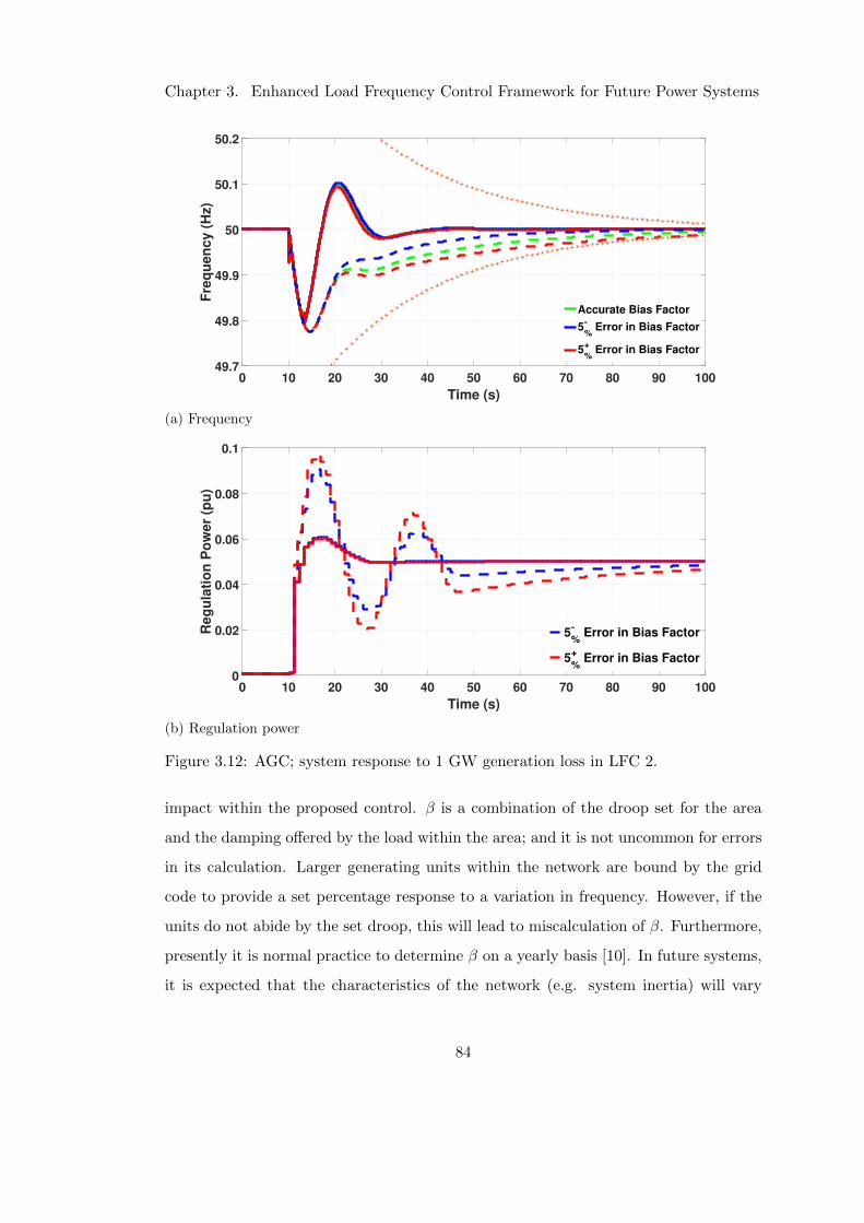
Chapter 3. Enhanced Load Frequency Control Framework for Future Power Systems
0 10 20 30 40 50 60 70 80 90 100
Time (s)
49.7
49.8
49.9
50
50.1
50.2
Fre
qu
en
cy
(H
z)
Accurate Bias Factor
5-
% Error in Bias Factor
5+
% Error in Bias Factor
(a) Frequency
0 10 20 30 40 50 60 70 80 90 100
Time (s)
0
0.02
0.04
0.06
0.08
0.1
Re
gu
lati
on
Po
we
r (p
u)
5-
% Error in Bias Factor
5+
% Error in Bias Factor
(b) Regulation power
Figure 3.12: AGC; system response to 1 GW generation loss in LFC 2.
impact within the proposed control. β is a combination of the droop set for the area
and the damping offered by the load within the area; and it is not uncommon for errors
in its calculation. Larger generating units within the network are bound by the grid
code to provide a set percentage response to a variation in frequency. However, if the
units do not abide by the set droop, this will lead to miscalculation of β. Furthermore,
presently it is normal practice to determine β on a yearly basis [10]. In future systems,
it is expected that the characteristics of the network (e.g. system inertia) will vary
84
Chapter 3. Enhanced Load Frequency Control Framework for Future Power Systems
vastly within a single day. It is also expected that the difference between the peak load
and the base load will increase significantly [19], thereby resulting in the load offering
a different damping effect at different times. Therefore, the proposed control utilising
∆P tie is more resilient to changes expected within the future power system.
Furthermore, if ACE is utilised within the BCL of the proposed framework, although
the activations of reserves are guaranteed to be unilateral within the area where distur-
bance has been detected, the miscalculation of β leads to nuisance activations as shown
in Fig. 3.12b. It should be noted that utilising ∆P tie avoids any nuisance activations.
3.7 Conclusions
In response to the research questions set forth in Chapter 2, this chapter investigates
enhanced responsibilisation for secondary frequency control. To this end, the approach,
key conclusions and findings are summarised below:
• The modeling of conventional LFC framework was presented, followed by its in-
corporation within the validated reduced dynamic model of GB reference power
system. The baseline simulation results revealed a satisfactory frequency re-
sponse. The incorporation of conventional LFC framework within the GB grid
begins to introduce a degree of decentralisation and responsibilisation. Remedial
measures are taken closer to the location of the imbalance event, i.e., within the
area of the disturbance as opposed to the current practice within GB grid where
the response is from across GB. To the best of authors knowledge, this is the first
implementation where the conventional LFC framework has been incorporated
within the GB grid.
• An analysis of the conventional LFC framework response revealed that the two
objectives set in Chapter 2, i.e., improved responsibilisation and improved re-
sponse speed, were contradictory to each other. An increase in response speed
of conventional LFC would lead to degrading responsibilisation. Furthermore, in
regards to the third objective of effective utilisation of fast acting demand side
85

Chapter 3. Enhanced Load Frequency Control Framework for Future Power Systems
devices within the network, it was found that although a large proportion of ac-
tivated secondary reserves were fast acting, the speed of response of such devices
did not contribute to frequency restoration speed. Further analysis identified
practical limitations that lead to conflicting objectives. These limitations are:
– Lack of fast and definitive identification of the location of imbalance.
– A common control effort for both CGs, that may have a ramp-rate constraint
and fast acting resources with no ramp-rate constraint.
• To overcome the limitations of the conventional approach, a novel SFC (EFC-FB)
is proposed. The control incorporates a fast acting balance control loop (BCL),
in addition to the secondary control loop. The key features of the proposed
framework are:
– It incorporates an area disturbance observer capable of fast, autonomous
and definitive identification of location of the imbalance.
– The impact of definitive identification of location of imbalance is two-fold:
(i) it ensures unilateral activation of reserves only within the LFC area where
the imbalance initiated, allowing faster response speed, and (ii) enables use
of area power imbalance observed over tie-lines as control input as opposed to
conventionally utilised area control error, avoiding sympathetic activations
due to faster response speeds.
– Decouples the control effort of fast acting resources from that of CGs. The
control effort to fast acting resources is a combination of effort from BCL
and secondary control loop, while the control effort to CGs is from secondary
control loop only.
• The results of real-time simulations and small-signal analysis conducted on the
reduced dynamic model of GB presented within this chapter provides a high
degree of confidence in the performance of the proposed control. This chapter
further presents a justification, informed by simulation and small-signal analysis
results, of design choices of the proposed control. It should be noted that al-
86
Chapter 3. Enhanced Load Frequency Control Framework for Future Power Systems
though no offline simulations have been undertaken in this work, they serve an
important role in large scale representative studies of the power system for both
theoretical and practical applications. One such example is the determination
of accurate/realistic value of load damping characteristic D under varying load
composition. Detailed modelling of a power system is made possible by offline
simulation tools that do not have restrictions such as the computational effort in
clock time imposed on real-time simulators.
• The work presented in this chapter effectively works towards addressing the re-
search questions and objectives set in Chapter 2. The proposed control enables
fast response speeds while at the same time ensuring effective, improved respon-
sibilisation. In addition, the EFC-FB enables effective utilisation of fast acting
devices, allowing for their fast response speed to contribute to frequency restora-
tion time.
87

Chapter 3. Enhanced Load Frequency Control Framework for Future Power Systems
REFERENCES
[1] “Electricity Ten Year Statement 2016”, National Grid, 2016. [On-
line]. Available: http://www2.nationalgrid.com/UK/Industry-information/
Future-of-Energy/Electricity-ten-year-statement
[2] P. Kundur, “Control of Active Power and Reactive Power”, in Power System
Stability and Control, McGraw-Hill, Inc., ch. 11, sec. 11.1.6, pp. 617-623.
[3] X. Jun and A. Dysko,“UK transmission system modelling and validation for dy-
namic studies”, in proceedings of 4ˆth IEEE PES Innovative Smart Grid Tech-
nologies (ISGT Europe), Lyngby, Denmark, pp. 1-5, 2013.
[4] A. Emhemed, et al., “Studies of dynamic interactions in hybrid ac-dc grid under
different fault conditions using real time digital simulation”, in proceedings of
the 13ˆth IET International conference on AC and DC Power Transmission,
Manchester, pp. 1-5, 2017.
[5] “Policy P1: Load-Frequency Control and Performance”, in Continental
Europe Operation Handbook, ENTSO-E, 2016. [Online]. Available:https:
//www.entsoe.eu/publications/system-operations-reports/operation-handbook/
Pages/default.aspx
[6] “Electricity Capacity Assessment Report”, ofgem, 2013. [On-
line]. Available:https://www.ofgem.gov.uk/ofgem-publications/75232/
electricity-capacity-assessment-report-2013-pdf
[7] “Wind energy implications of large scale deployment”, Royal Academy of En-
gineering, 2014. [Online]. Available:https://www.raeng.org.uk/publications/
reports/wind-energy-implications-of-large-scale-deployment
[8] “National Electricity Transmission System Performance Report 2015-2016 – Re-
port to the Gas and Electricity Markets Authority”, National Grid, 2016. [On-
line]. Available:http://www2.nationalgrid.com/WorkArea/DownloadAsset.aspx?
id=8589936830
88
Chapter 3. Enhanced Load Frequency Control Framework for Future Power Systems
[9] “Appendix 1: Load-Frequency Control and Performance”, in Continen-
tal Europe Operation Handbook, ENTSO-E, 2016. [Online]. Avail-
able: https://www.entsoe.eu/publications/system-operations-reports/
operation-handbook/Pages/default.aspx
[10] “Balancing and Frequency Control”, NERC, 2011. [Online]. Available:
http://www.nerc.com/docs/oc/rs/NERC%20Balancing%20and%20Frequency%
20Control%20040520111.pdf
[11] “The Power of Transformation – Wind, Sun and the Economics of
Flexible Power Systems”, International Energy Agency, 2014. [Online].
Available: https://www.iea.org/publications/freepublications/publication/The
power of Transformation.pdf
[12] C. K. Zhang, L. Jiang, Q. H. Wu, Y. He and M. Wu,“Delay-Dependent Robust
Load Frequency Control for Time Delay Power Systems”, in IEEE Trans. on
Power Systems, vol. 28, no. 3, pp. 2192-2201, Aug. 2013.
[13] K. S. Ko and D. K. Sung, “The Effect of Cellular Network-based Communication
Delays in an EV Aggregator’s Domain on Frequency Regulation Service”, in IEEE
Trans. on Smart Grid, vol. PP, no. 99, pp. 1-1.
[14] N. Lu et al, “Design Considerations of a Centralized Load Controller Using Ther-
mostatically Controlled Appliances for Continuous Regulation Reserves”, in IEEE
Trans. on Smart Grid, vol. 4, no. 2, June 2013.
[15] F. Ding, et. al, “Peak-ratio analysis method for enhancement of LOM protection
using M class PMUs”, in IEEE Trans. on Smart Grid, 2016, pp. 291-299.
[16] A. M. Prostejovsky, M. Marinelli, M. Rezkalla, M. H. Syed, and E. Guillo Sansano,
“Tuningless Load Frequency Control through Active Engagement of Distributed
Resources’ in IEEE Trans. on Power Systems, September 2017.
[17] “Report on the evaluation and validation of the ELECTRA WoC control concept”
ELECTRA IRP consortium, Deliverable D7.1, 2018.
89

Chapter 3. Enhanced Load Frequency Control Framework for Future Power Systems
[18] N. V. Ramana, “Two-Area Load Frequency Control”, in Power System Operation
and Control, Pearson Education India, ch. 6, pp. 115-131.
[19] “System Operability Framework 2016”, National Grid, 2016. [On-
line]. Available: http://www2.nationalgrid.com/UK/Industry-information/
Future-of-Energy/System-Operability-Framework
90
Chapter 4
Novel Decentralised Primary
Frequency Control: Introducing
Responsibilisation within
Primary Frequency Control
4.1 Introduction
Having improved the response speed of secondary frequency control (SFC) by means
of introducing enhanced responsibilisation in Chapter 3, this chapter works towards
achieving responsibilisation within primary frequency control (PFC).
This chapter is organised as follows: Section 4.2 presents the conventional PFC
modelling and its incorporation within reference power system. This is followed by
an evaluation of its responsibilisation capability. Section 4.3 discusses the approaches
established in literature for PFC responsibilisation. A novel decentralised PFC, where
responsibilisation is achieved by means of measuring the transient phase offset (TPO)
within each of the load frequency control (LFC) areas is proposed in Section 4.4. The
performance of the proposed control is verified by real-time simulations and corrobo-
rated by small-signal analysis in Section 4.5. Section 4.6 concludes the chapter.
91
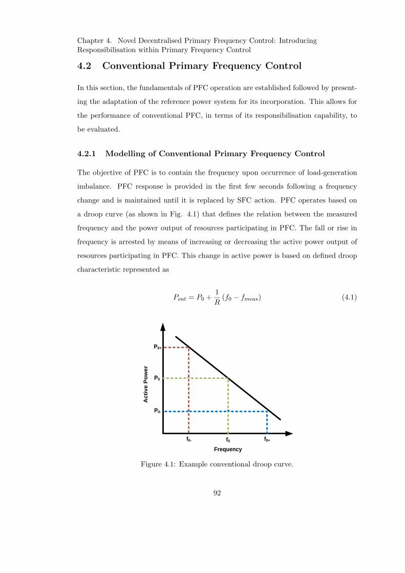
Chapter 4. Novel Decentralised Primary Frequency Control: IntroducingResponsibilisation within Primary Frequency Control
4.2 Conventional Primary Frequency Control
In this section, the fundamentals of PFC operation are established followed by present-
ing the adaptation of the reference power system for its incorporation. This allows for
the performance of conventional PFC, in terms of its responsibilisation capability, to
be evaluated.
4.2.1 Modelling of Conventional Primary Frequency Control
The objective of PFC is to contain the frequency upon occurrence of load-generation
imbalance. PFC response is provided in the first few seconds following a frequency
change and is maintained until it is replaced by SFC action. PFC operates based on
a droop curve (as shown in Fig. 4.1) that defines the relation between the measured
frequency and the power output of resources participating in PFC. The fall or rise in
frequency is arrested by means of increasing or decreasing the active power output of
resources participating in PFC. This change in active power is based on defined droop
characteristic represented as
Pout = P0 +1
R(f0 − fmeas) (4.1)
P0
f0
Ac
tiv
e P
ow
er
Frequency
f0+f0-
P0-
P0+
Figure 4.1: Example conventional droop curve.
92
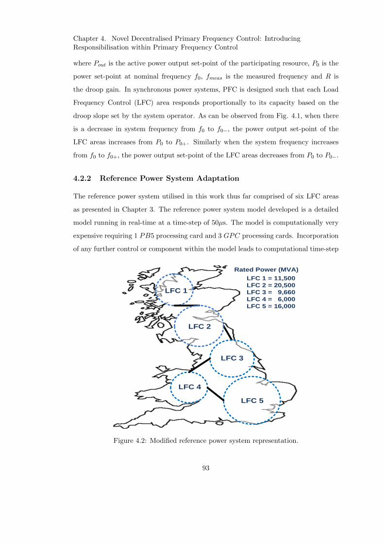
Chapter 4. Novel Decentralised Primary Frequency Control: IntroducingResponsibilisation within Primary Frequency Control
where Pout is the active power output set-point of the participating resource, P0 is the
power set-point at nominal frequency f0, fmeas is the measured frequency and R is
the droop gain. In synchronous power systems, PFC is designed such that each Load
Frequency Control (LFC) area responds proportionally to its capacity based on the
droop slope set by the system operator. As can be observed from Fig. 4.1, when there
is a decrease in system frequency from f0 to f0−, the power output set-point of the
LFC areas increases from P0 to P0+. Similarly when the system frequency increases
from f0 to f0+, the power output set-point of the LFC areas decreases from P0 to P0−.
4.2.2 Reference Power System Adaptation
The reference power system utilised in this work thus far comprised of six LFC areas
as presented in Chapter 3. The reference power system model developed is a detailed
model running in real-time at a time-step of 50µs. The model is computationally very
expensive requiring 1 PB5 processing card and 3 GPC processing cards. Incorporation
of any further control or component within the model leads to computational time-step
LFC 1
LFC 2
LFC 5
LFC 3
LFC 4
Rated Power (MVA)
LFC 1 = 11,500
LFC 2 = 20,500
LFC 3 = 9,660
LFC 4 = 6,000
LFC 5 = 16,000
Figure 4.2: Modified reference power system representation.
93
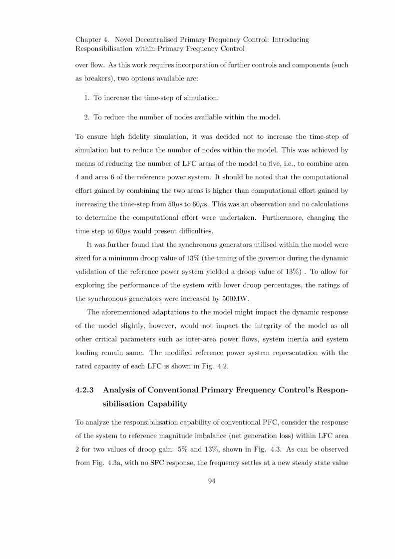
Chapter 4. Novel Decentralised Primary Frequency Control: IntroducingResponsibilisation within Primary Frequency Control
over flow. As this work requires incorporation of further controls and components (such
as breakers), two options available are:
1. To increase the time-step of simulation.
2. To reduce the number of nodes available within the model.
To ensure high fidelity simulation, it was decided not to increase the time-step of
simulation but to reduce the number of nodes within the model. This was achieved by
means of reducing the number of LFC areas of the model to five, i.e., to combine area
4 and area 6 of the reference power system. It should be noted that the computational
effort gained by combining the two areas is higher than computational effort gained by
increasing the time-step from 50µs to 60µs. This was an observation and no calculations
to determine the computational effort were undertaken. Furthermore, changing the
time step to 60µs would present difficulties.
It was further found that the synchronous generators utilised within the model were
sized for a minimum droop value of 13% (the tuning of the governor during the dynamic
validation of the reference power system yielded a droop value of 13%) . To allow for
exploring the performance of the system with lower droop percentages, the ratings of
the synchronous generators were increased by 500MW.
The aforementioned adaptations to the model might impact the dynamic response
of the model slightly, however, would not impact the integrity of the model as all
other critical parameters such as inter-area power flows, system inertia and system
loading remain same. The modified reference power system representation with the
rated capacity of each LFC is shown in Fig. 4.2.
4.2.3 Analysis of Conventional Primary Frequency Control’s Respon-
sibilisation Capability
To analyze the responsibilisation capability of conventional PFC, consider the response
of the system to reference magnitude imbalance (net generation loss) within LFC area
2 for two values of droop gain: 5% and 13%, shown in Fig. 4.3. As can be observed
from Fig. 4.3a, with no SFC response, the frequency settles at a new steady state value
94
Chapter 4. Novel Decentralised Primary Frequency Control: IntroducingResponsibilisation within Primary Frequency Control
0 10 20 30 40 50 60 70 80 90 100
Time (s)
49.75
49.8
49.85
49.9
49.95
50
50.05
Fre
qu
en
cy (
Hz)
Frequency 13% Fixed Droop
Frequency 5% Fixed Droop
(a) Frequency.
0 10 20 30 40 50 60 70 80 90 100
Time (s)
0
100
200
300
400
500
Po
wer
(MW
)
LFC 1 LFC 2 LFC 3 LFC 4 LFC 5
(b) PFC response.
Figure 4.3: System PFC response to 1000MW generation loss.
after the imbalance. In accordance with droop response, the frequency settles at two
different values for the two different droop gains utilised. A 5% droop gain corresponds
to a higher PFC response and therefore the frequency settles at a higher value than
compared to with droop gain of 13%. However, it should be noted that although
two different values of droop gains have been utilised, for a disturbance of reference
magnitude, the contribution of active power from each of the LFC area remains same
and proportional to the capacity of individual LFC area as shown in Fig. 4.3b. For
further evaluation, reference magnitude imbalance is emulated in each of the LFC areas
individually with a variation in droop gain from 13% to 5%. The droop is varied in
95

Chapter 4. Novel Decentralised Primary Frequency Control: IntroducingResponsibilisation within Primary Frequency Control
Area 1
12
34
5
Area5
10
15
Droop (%)
174
175
176
Po
ut
Area 2
12
34
5
Area5
10
15
Droop (%)
325
326
327
Po
ut
Area 3
12
34
5
Area5
10
15
Droop (%)
148
149
150
Po
ut
Area 4
12
34
5
Area5
10
15
Droop (%)
89
90
91
Po
ut
Area 5
12
34
5
Area5
10
15
Droop (%)
259
260
261
Po
ut
Figure 4.4: Individual LFC areas’ contribution to PFC
steps of 1% for all the LFC areas, i.e, if the droop value is 6%, it is 6% for all the LFC
areas. The increase in power output of individual LFC area, i.e., the PFC response
of each LFC area, is presented in Fig. 4.4. As can be observed, irrespective of the
location of the imbalance event or the value of droop gain chosen (as long as it is same
for each area), the PFC response of each LFC area remains same, i.e., proportional to
the capacity of the LFC area.
From the analysis presented above, it can therefore be inferred that there is no
inherent responsibilisation within the conventional PFC as there is in conventional
SFC.
4.3 Responsibilising Primary Frequency Control
Introducing responsibilisation within PFC of synchronous power systems refers to en-
forcing the LFC area with an imbalance event to contribute more PFC response to the
96
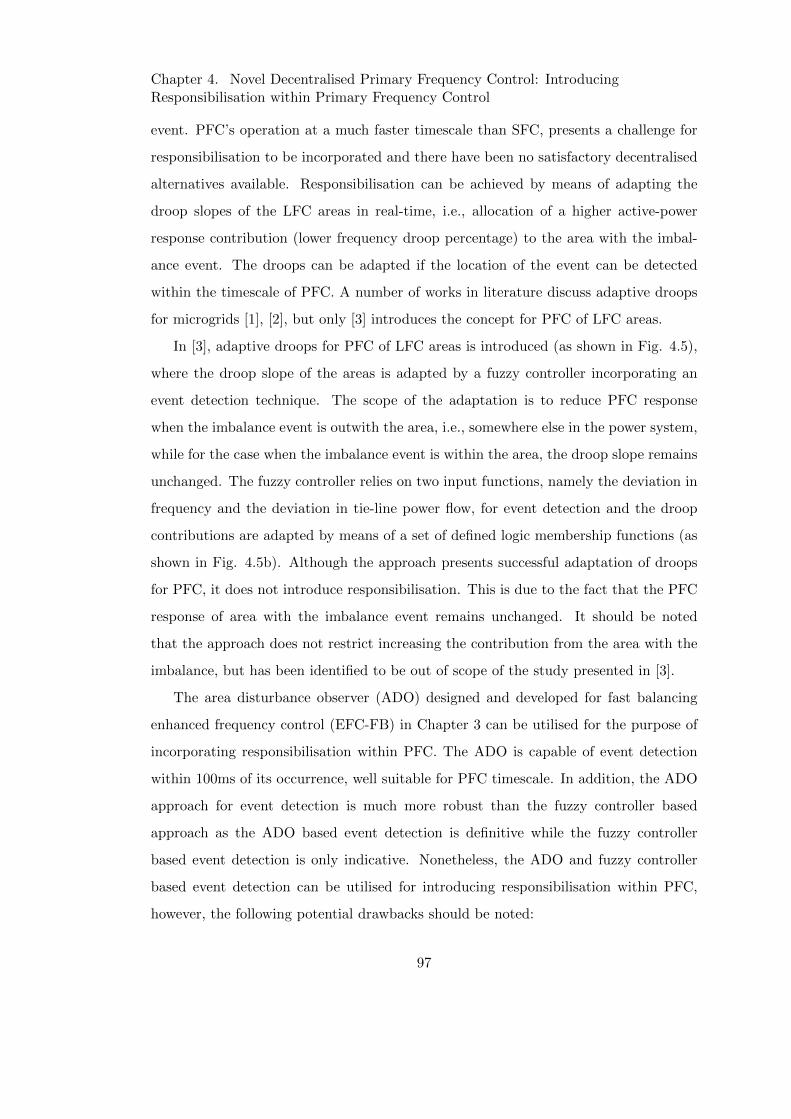
Chapter 4. Novel Decentralised Primary Frequency Control: IntroducingResponsibilisation within Primary Frequency Control
event. PFC’s operation at a much faster timescale than SFC, presents a challenge for
responsibilisation to be incorporated and there have been no satisfactory decentralised
alternatives available. Responsibilisation can be achieved by means of adapting the
droop slopes of the LFC areas in real-time, i.e., allocation of a higher active-power
response contribution (lower frequency droop percentage) to the area with the imbal-
ance event. The droops can be adapted if the location of the event can be detected
within the timescale of PFC. A number of works in literature discuss adaptive droops
for microgrids [1], [2], but only [3] introduces the concept for PFC of LFC areas.
In [3], adaptive droops for PFC of LFC areas is introduced (as shown in Fig. 4.5),
where the droop slope of the areas is adapted by a fuzzy controller incorporating an
event detection technique. The scope of the adaptation is to reduce PFC response
when the imbalance event is outwith the area, i.e., somewhere else in the power system,
while for the case when the imbalance event is within the area, the droop slope remains
unchanged. The fuzzy controller relies on two input functions, namely the deviation in
frequency and the deviation in tie-line power flow, for event detection and the droop
contributions are adapted by means of a set of defined logic membership functions (as
shown in Fig. 4.5b). Although the approach presents successful adaptation of droops
for PFC, it does not introduce responsibilisation. This is due to the fact that the PFC
response of area with the imbalance event remains unchanged. It should be noted
that the approach does not restrict increasing the contribution from the area with the
imbalance, but has been identified to be out of scope of the study presented in [3].
The area disturbance observer (ADO) designed and developed for fast balancing
enhanced frequency control (EFC-FB) in Chapter 3 can be utilised for the purpose of
incorporating responsibilisation within PFC. The ADO is capable of event detection
within 100ms of its occurrence, well suitable for PFC timescale. In addition, the ADO
approach for event detection is much more robust than the fuzzy controller based
approach as the ADO based event detection is definitive while the fuzzy controller
based event detection is only indicative. Nonetheless, the ADO and fuzzy controller
based event detection can be utilised for introducing responsibilisation within PFC,
however, the following potential drawbacks should be noted:
97
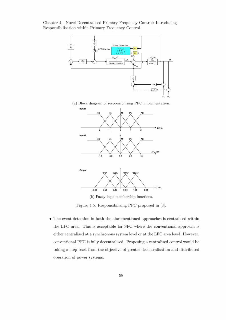
Chapter 4. Novel Decentralised Primary Frequency Control: IntroducingResponsibilisation within Primary Frequency Control
(a) Block diagram of responsibilising PFC implementation.
(b) Fuzzy logic membership functions.
Figure 4.5: Responsibilising PFC proposed in [3].
• The event detection in both the aforementioned approaches is centralised within
the LFC area. This is acceptable for SFC where the conventional approach is
either centralised at a synchronous system level or at the LFC area level. However,
conventional PFC is fully decentralised. Proposing a centralised control would be
taking a step back from the objective of greater decentralisation and distributed
operation of power systems.
98
Chapter 4. Novel Decentralised Primary Frequency Control: IntroducingResponsibilisation within Primary Frequency Control
• Although the event detection by fuzzy based control is only indicative, its perfor-
mance for PFC has been shown to be satisfactory in [3]. However, the appraisal of
the approach does not incorporate communication delays. It is important to note
that once the event has been identified, the new values of droop percentages do
need to be communicated to the resources participating in PFC. Therefore, the
performance of the approach relies extensively on communication infrastructure.
• The above approaches require more observables than that utilised by present day
PFC, and therefore would be subject to higher measurement uncertainty.
4.4 Proposed Novel Decentralised Responsibilising Pri-
mary Frequency Control
This work proposes an alternative novel decentralised PFC, referred to as the respon-
sibilising primary enhanced frequency control (EFC-RP), where responsibilisation is
achieved by means of measuring the TPO within each of the LFC areas. The pro-
posed approach is fully decentralised as it relies on a single local measurement only
and requires no form of communication. In the following sub-sections, the TPO based
method of responsibilisation is presented.
4.4.1 Fast Event Location Detection by Transient Phase Offset
Any sudden imbalance between generator mechanical power and load leads to a per-
ceived change in frequency, in high or low inertia systems, due to the changing phase
angles across network impedances, as active power flows change. The local Rate of
Change of Frequency (RoCoF ) in response to sudden imbalance can be approximated
as [4]:
RoCoF =∆P · f
2 ·G ·HHz/s (4.2)
where ∆P is the change in active power output, f is the system frequency, G is the
nominal generator rating of the area under consideration and H is the inertia constant
99
Chapter 4. Novel Decentralised Primary Frequency Control: IntroducingResponsibilisation within Primary Frequency Control
of the generator of the area under consideration. The local RoCoF at time instant k
can then be measured as [4]:
RoCoF =fk − f(k−T )
THz/s (4.3)
where T represents the measurement window length. Essentially, RoCoF is an estimate
of local double derivative of the phase angle φ over the window T , obtainable by:
f =dφ
dt(4.4)
0 10 20 30 40 50 60 70 80 90 100
Time (s)
49.8
49.9
50
Fre
qu
en
cy (
Hz)
Frequency LFC 1
Frequency LFC 2
Frequency LFC 3
Frequency LFC 4
Frequency LFC 5
9.98 10 10.02 10.04 10.06 10.08 10.149.95
50
(a) Frequency.
10 10.02 10.04 10.06 10.08 10.1
Time (s)
0
1
2
3
4
5
6
TP
O (
Deg
rees)
TPO LFC 1
TPO LFC 2
TPO LFC 3
TPO LFC 4
TPO LFC 5
(b) TPO.
Figure 4.6: System Response to 1000 MW Generation Loss.
100
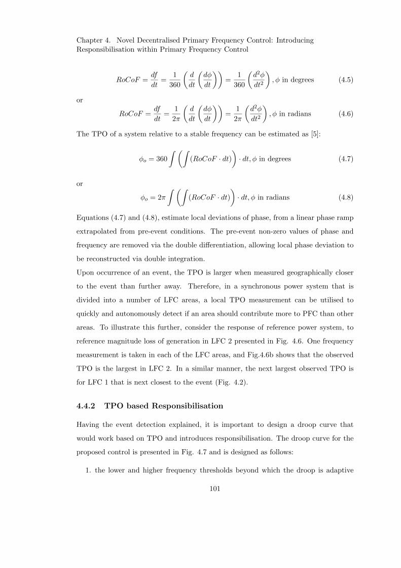
Chapter 4. Novel Decentralised Primary Frequency Control: IntroducingResponsibilisation within Primary Frequency Control
RoCoF =df
dt=
1
360
(d
dt
(dφ
dt
))=
1
360
(d2φ
dt2
), φ in degrees (4.5)
or
RoCoF =df
dt=
1
2π
(d
dt
(dφ
dt
))=
1
2π
(d2φ
dt2
), φ in radians (4.6)
The TPO of a system relative to a stable frequency can be estimated as [5]:
φo = 360
∫ (∫(RoCoF · dt)
)· dt, φ in degrees (4.7)
or
φo = 2π
∫ (∫(RoCoF · dt)
)· dt, φ in radians (4.8)
Equations (4.7) and (4.8), estimate local deviations of phase, from a linear phase ramp
extrapolated from pre-event conditions. The pre-event non-zero values of phase and
frequency are removed via the double differentiation, allowing local phase deviation to
be reconstructed via double integration.
Upon occurrence of an event, the TPO is larger when measured geographically closer
to the event than further away. Therefore, in a synchronous power system that is
divided into a number of LFC areas, a local TPO measurement can be utilised to
quickly and autonomously detect if an area should contribute more to PFC than other
areas. To illustrate this further, consider the response of reference power system, to
reference magnitude loss of generation in LFC 2 presented in Fig. 4.6. One frequency
measurement is taken in each of the LFC areas, and Fig.4.6b shows that the observed
TPO is the largest in LFC 2. In a similar manner, the next largest observed TPO is
for LFC 1 that is next closest to the event (Fig. 4.2).
4.4.2 TPO based Responsibilisation
Having the event detection explained, it is important to design a droop curve that
would work based on TPO and introduces responsibilisation. The droop curve for the
proposed control is presented in Fig. 4.7 and is designed as follows:
1. the lower and higher frequency thresholds beyond which the droop is adaptive
101
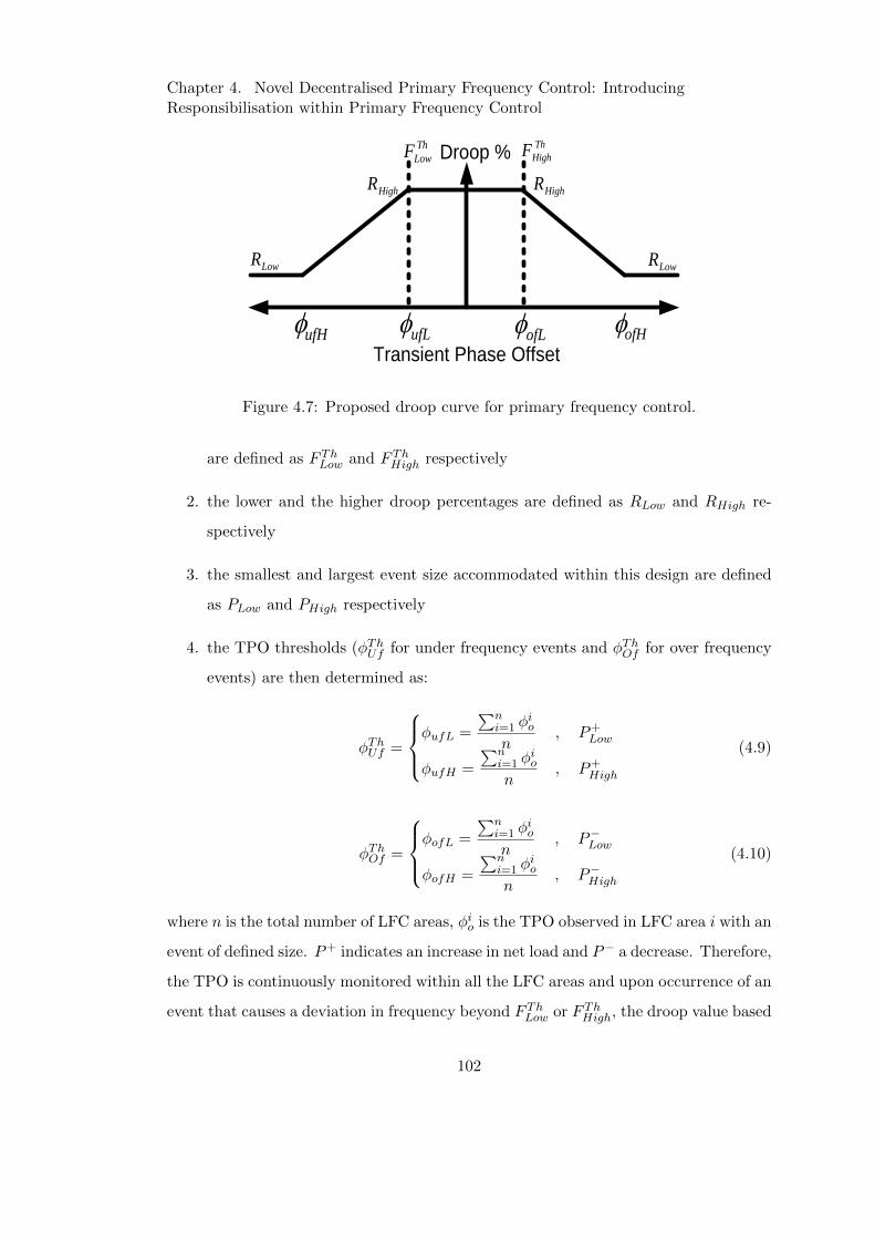
Chapter 4. Novel Decentralised Primary Frequency Control: IntroducingResponsibilisation within Primary Frequency Control
Droop %
Transient Phase Offset
HighR
LowR
ufH
Th
LowFTh
HighF
ufL ofHofL
LowR
HighR
Figure 4.7: Proposed droop curve for primary frequency control.
are defined as F ThLow and F ThHigh respectively
2. the lower and the higher droop percentages are defined as RLow and RHigh re-
spectively
3. the smallest and largest event size accommodated within this design are defined
as PLow and PHigh respectively
4. the TPO thresholds (φThUf for under frequency events and φThOf for over frequency
events) are then determined as:
φThUf =
φufL =
∑ni=1 φ
io
n, P+
Low
φufH =
∑ni=1 φ
io
n, P+
High
(4.9)
φThOf =
φofL =
∑ni=1 φ
io
n, P−Low
φofH =
∑ni=1 φ
io
n, P−High
(4.10)
where n is the total number of LFC areas, φio is the TPO observed in LFC area i with an
event of defined size. P+ indicates an increase in net load and P− a decrease. Therefore,
the TPO is continuously monitored within all the LFC areas and upon occurrence of an
event that causes a deviation in frequency beyond F ThLow or F ThHigh, the droop value based
102
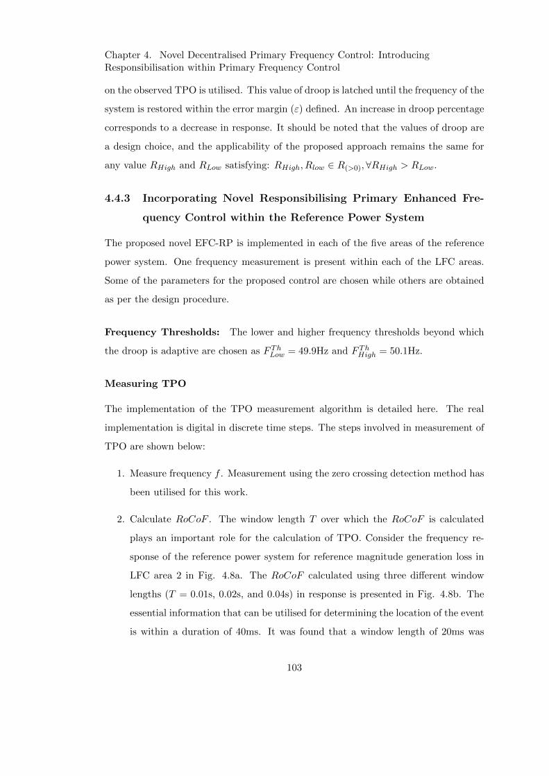
Chapter 4. Novel Decentralised Primary Frequency Control: IntroducingResponsibilisation within Primary Frequency Control
on the observed TPO is utilised. This value of droop is latched until the frequency of the
system is restored within the error margin (ε) defined. An increase in droop percentage
corresponds to a decrease in response. It should be noted that the values of droop are
a design choice, and the applicability of the proposed approach remains the same for
any value RHigh and RLow satisfying: RHigh, Rlow ∈ R(>0),∀RHigh > RLow.
4.4.3 Incorporating Novel Responsibilising Primary Enhanced Fre-
quency Control within the Reference Power System
The proposed novel EFC-RP is implemented in each of the five areas of the reference
power system. One frequency measurement is present within each of the LFC areas.
Some of the parameters for the proposed control are chosen while others are obtained
as per the design procedure.
Frequency Thresholds: The lower and higher frequency thresholds beyond which
the droop is adaptive are chosen as F ThLow = 49.9Hz and F ThHigh = 50.1Hz.
Measuring TPO
The implementation of the TPO measurement algorithm is detailed here. The real
implementation is digital in discrete time steps. The steps involved in measurement of
TPO are shown below:
1. Measure frequency f . Measurement using the zero crossing detection method has
been utilised for this work.
2. Calculate RoCoF . The window length T over which the RoCoF is calculated
plays an important role for the calculation of TPO. Consider the frequency re-
sponse of the reference power system for reference magnitude generation loss in
LFC area 2 in Fig. 4.8a. The RoCoF calculated using three different window
lengths (T = 0.01s, 0.02s, and 0.04s) in response is presented in Fig. 4.8b. The
essential information that can be utilised for determining the location of the event
is within a duration of 40ms. It was found that a window length of 20ms was
103
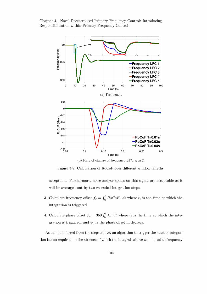
Chapter 4. Novel Decentralised Primary Frequency Control: IntroducingResponsibilisation within Primary Frequency Control
0 10 20 30 40 50 60 70 80 90 100
Time (s)
49.8
49.9
50
Fre
qu
en
cy (
Hz)
Frequency LFC 1
Frequency LFC 2
Frequency LFC 3
Frequency LFC 4
Frequency LFC 5
9.98 10 10.02 10.04 10.06 10.08 10.149.95
50
(a) Frequency.
0.05 0.1 0.15 0.2 0.25 0.3
Time (s)
-1.2
-1
-0.8
-0.6
-0.4
-0.2
0
0.2
Ro
Co
F (
Hz/s
)
RoCoF T=0.01s
RoCoF T=0.02s
RoCoF T=0.04s
(b) Rate of change of frequency LFC area 2.
Figure 4.8: Calculation of RoCoF over different window lengths.
acceptable. Furthermore, noise and/or spikes on this signal are acceptable as it
will be averaged out by two cascaded integration steps.
3. Calculate frequency offset fo =∫ tttRoCoF · dt where tt is the time at which the
integration is triggered.
4. Calculate phase offset φo = 360∫ tttfo · dt where tt is the time at which the inte-
gration is triggered, and φo is the phase offset in degrees.
As can be inferred from the steps above, an algorithm to trigger the start of integra-
tion is also required; in the absence of which the integrals above would lead to frequency
104
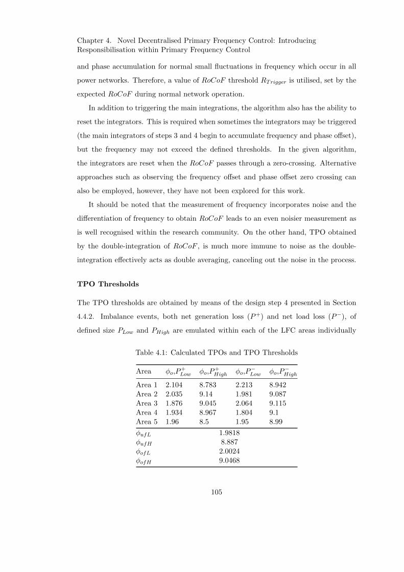
Chapter 4. Novel Decentralised Primary Frequency Control: IntroducingResponsibilisation within Primary Frequency Control
and phase accumulation for normal small fluctuations in frequency which occur in all
power networks. Therefore, a value of RoCoF threshold RTrigger is utilised, set by the
expected RoCoF during normal network operation.
In addition to triggering the main integrations, the algorithm also has the ability to
reset the integrators. This is required when sometimes the integrators may be triggered
(the main integrators of steps 3 and 4 begin to accumulate frequency and phase offset),
but the frequency may not exceed the defined thresholds. In the given algorithm,
the integrators are reset when the RoCoF passes through a zero-crossing. Alternative
approaches such as observing the frequency offset and phase offset zero crossing can
also be employed, however, they have not been explored for this work.
It should be noted that the measurement of frequency incorporates noise and the
differentiation of frequency to obtain RoCoF leads to an even noisier measurement as
is well recognised within the research community. On the other hand, TPO obtained
by the double-integration of RoCoF , is much more immune to noise as the double-
integration effectively acts as double averaging, canceling out the noise in the process.
TPO Thresholds
The TPO thresholds are obtained by means of the design step 4 presented in Section
4.4.2. Imbalance events, both net generation loss (P+) and net load loss (P−), of
defined size PLow and PHigh are emulated within each of the LFC areas individually
Table 4.1: Calculated TPOs and TPO Thresholds
Area φo,P+Low φo,P
+High φo,P
−Low φo,P
−High
Area 1 2.104 8.783 2.213 8.942Area 2 2.035 9.14 1.981 9.087Area 3 1.876 9.045 2.064 9.115Area 4 1.934 8.967 1.804 9.1Area 5 1.96 8.5 1.95 8.99
φufL 1.9818φufH 8.887φofL 2.0024φofH 9.0468
105
Chapter 4. Novel Decentralised Primary Frequency Control: IntroducingResponsibilisation within Primary Frequency Control
and the TPO is calculated. The TPO of each LFC for P+Low, P+
Highi and P−Low , P−High
are tabulated in Table: 4.1. As per the design procedure, averaging the calculated
TPOs of all areas, the TPO thresholds are obtained as φufL= 2, φufH= 9, φofL= 2
and φofH= 9 (rounded to nearest integer).
Droop Range: In the validation of the reference power system, the droop value was
observed as 13% [6]. In general, ENTSO-E recommends a droop value in the range
of 2-12% [7]. Assuming that 13% would be the maximum value of droop within the
reference power system and the typical value of droop identified as 5% in [8], the droop
values were chosen as RLow = 5% and RHigh = 13%.
Event Size: The smallest and the largest event size need to be defined for obtaining
the TPO thresholds. The smallest event size is chosen as three times the expected
load change while the largest event size is according to N-1 contingency planning. For
the given study, the values are chosen as PLow = 500MW and PHigh = 1800MW. To
be consistent with the remainder of the thesis, in this chapter the performance of the
proposed control will be evaluated for the reference event, i.e., 1000MW in size.
4.5 Performance Evaluation of Proposed Novel Responsi-
bilising Primary Enhanced Frequency Control
In this section, the applicability of the proposed novel EFC-RP is validated by means
of real-time simulations.
Methodology: The performance of the proposed novel EFC-RP is compared to that
of conventional PFC by means of the following defined scenario:
Response to Reference Imbalance Event: The system is subject to one distur-
bance, net loss of generation of reference magnitude.
To aid the assessment, one key indicator is defined as:
• Percentage Change in Primary Frequency Control Response (∆PCPFC):
∆PCPFC is defined as the percentage change (increase or decrease) in PFC re-
106
Chapter 4. Novel Decentralised Primary Frequency Control: IntroducingResponsibilisation within Primary Frequency Control
sponse of individual LFC area subject to an imbalance event compared to that
of conventional PFC approach where fixed droops for all LFC areas are utilised
and can be calculated as :
∆PCPFC =∆PPPFCPFC −∆PCPFCPFC
∆PCPFCPFC
100% (4.11)
where ∆PPPFCPFC is the PFC response with proposed PFC and ∆PCPFCPFC is the
PFC response with conventional PFC.
In addition to the evaluation of proposed EFC-RP performance, this section further
presents a small-signal stability analysis to affirm the applicability of the approach in
conjunction with SFC.
4.5.1 Response to Imbalance Event
The system response subject to reference magnitude generation loss at t = 10s is
presented in Fig. 4.9. The system frequency response is shown in Fig. 4.9a to be stable
and between fixed droop response of RLow and RHigh. The PFC response, i.e., the
active power contribution of each LFC, and change in droop of each LFC are presented
in Fig. 4.9b and Fig. 4.9c. As can be observed, the change in droop is within 1s
of the occurrence of the event. The solid line represents the system response with
fixed droop and the dotted line represents system response with the proposed control.
LFC area 2 increases its PFC response contribution to the event, demonstrating greater
responsibilisation. In a similar manner, LFC area 1 (that is next closest to the imbalance
event) increases its PFC response while all the other LFC areas decrease their PFC
response. The percentage change in PFC response of all the areas is shown in Fig.
4.10a
To further evaluate the performance of the proposed control and to demonstrate its
applicability, the imbalance event is emulated in each of the LFC areas individually.
The change in PFC response of each LFC area for the above scenarios are shown in Fig.
4.10b. Within a synchronous area A and for area under consideration i, defining the
neighborhood as NHi = {i,AN i} ⊆ A, with j ∈ AN i as adjacent areas coupled over
107
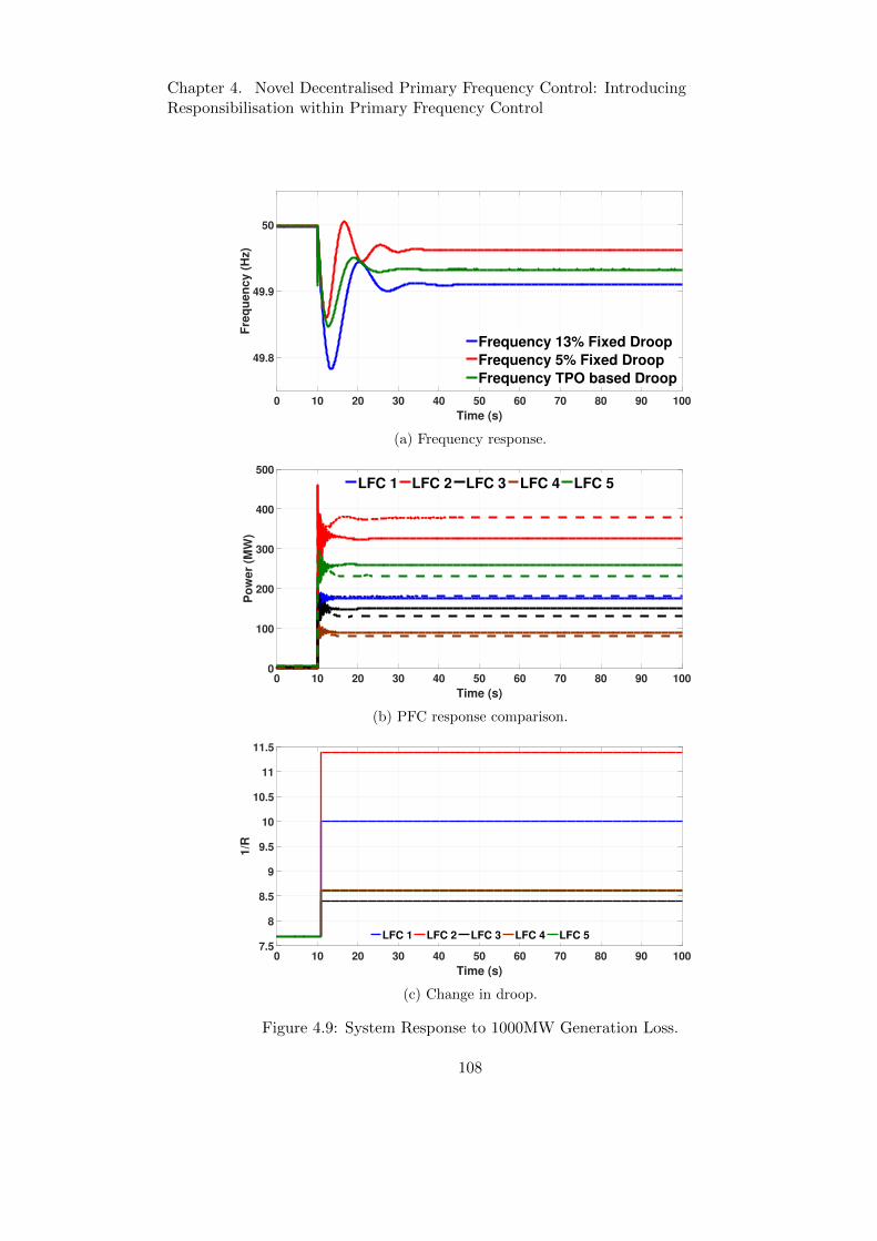
Chapter 4. Novel Decentralised Primary Frequency Control: IntroducingResponsibilisation within Primary Frequency Control
0 10 20 30 40 50 60 70 80 90 100
Time (s)
49.8
49.9
50
Fre
qu
en
cy (
Hz)
Frequency 13% Fixed Droop
Frequency 5% Fixed Droop
Frequency TPO based Droop
(a) Frequency response.
0 10 20 30 40 50 60 70 80 90 100
Time (s)
0
100
200
300
400
500
Po
wer
(MW
)
LFC 1 LFC 2 LFC 3 LFC 4 LFC 5
(b) PFC response comparison.
0 10 20 30 40 50 60 70 80 90 100
Time (s)
7.5
8
8.5
9
9.5
10
10.5
11
11.5
1/R
LFC 1 LFC 2 LFC 3 LFC 4 LFC 5
(c) Change in droop.
Figure 4.9: System Response to 1000MW Generation Loss.
108

Chapter 4. Novel Decentralised Primary Frequency Control: IntroducingResponsibilisation within Primary Frequency Control
tie-lines with breaker state δij , it can be observed that for an event in area i, in most
cases there is increase in PFC response from {i, j} and a decrease from {A −NHi}.
This study therefore demonstrates the ability of the proposed control to introduce
responsibilisation within PFC and serves as a proof of concept.
4.5.2 Small Signal Analysis
It is essential to assess the stability of a system with the proposed EFC-RP operating
in conjunction with SFC. In this sub-section, the stability is assessed by means of a
Area 1 Area 2 Area 3 Area 4 Area 5-15
-10
-5
0
5
10
15
20
Ch
an
ge in
PF
C R
esp
on
se (
%)
(a) Percentage change in PFC response.
Area 1 Area 2 Area 3 Area 4 Area 5-15
-10
-5
0
5
10
15
20
Ch
an
ge
in
PF
C R
es
po
ns
e (
%)
Event Area 1 Event Area 2 Event Area 3 Event Area 4 Event Area 5
(b) A snapshot of change in PFC response for events in individual LFC areas
Figure 4.10: Analysis of System Response to 1000 MW Generation Loss.
109

Chapter 4. Novel Decentralised Primary Frequency Control: IntroducingResponsibilisation within Primary Frequency Control
small-signal analysis. Small-signal analysis affirms the soundness and feasibility of the
approach. As highlighted by [9], small-signal analysis is a pragmatic approach, results
of which are of great practical relevance.
The system frequency response model of an n-area interconnected power system
is presented in Fig. 4.11. It should be noted that the model is similar to the model
utilised for small-signal analysis in the previous chapter, but not the same. For the
purpose of simplicity, only the conventional SFC is considered. The state-space model
of n-area system can be represented as [10]:
x = Ax+Bu+ Fw
y = Cx
(4.12)
where the state vector
x = [x1, x2, x3, x4]T (4.13)
the control vector
u = [δP rCGs1, . . . , δPrCGsn]T (4.14)
the disturbance vector
w = [∆PD1, . . . ,∆PDn]T (4.15)
ACEi
+
+
iiR/1
)(sPIi
-)(sMi
Governor
Turbine
s/2
ii DsH 2
1
Rotating Mass
and Load
+
PCEi
if
-
+
miP
DiP
n
ijj
ijT,1
+
-
-
PI
Controller
δPri
Coupling with
other areas
j
n
ijj
ij fT ,1
Figure 4.11: n-area interconnected power system frequency response model.
110
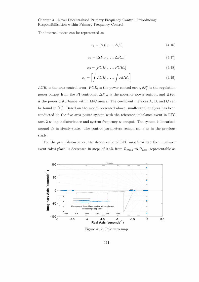
Chapter 4. Novel Decentralised Primary Frequency Control: IntroducingResponsibilisation within Primary Frequency Control
The internal states can be represented as
x1 = [∆f1, . . . ,∆fn] (4.16)
x2 = [∆Pm1, . . . ,∆Pmn] (4.17)
x3 = [PCE1, . . . , PCEn] (4.18)
x4 =
[∫ACE1, . . . ,
∫ACEn
](4.19)
ACEi is the area control error, PCEi is the power control error, δP ri is the regulation
power output from the PI controller, ∆Pmi is the governor power output, and ∆PDi
is the power disturbance within LFC area i. The coefficient matrices A, B, and C can
be found in [10]. Based on the model presented above, small-signal analysis has been
conducted on the five area power system with the reference imbalance event in LFC
area 2 as input disturbance and system frequency as output. The system is linearised
around f0 in steady-state. The control parameters remain same as in the previous
study.
For the given disturbance, the droop value of LFC area 2, where the imbalance
event takes place, is decreased in steps of 0.5% from RHigh to RLow, representable as
Pole-Zero Map
Real Axis (seconds-1)
Ima
gin
ary
Ax
is (
se
co
nd
s-1
)
-3 -2.5 -2 -1.5 -1 -0.5 0 0.5-100
-50
0
50
100
100
0.0030.00650.010.0150.0210.03
0.05
0.1
0.0030.00650.010.0150.0210.03
0.05
0.1
20
40
60
80
100
20
40
60
80
Real Axis (seconds-1
)
Ima
gin
ary
Ax
is (
se
co
nd
s-1
)
-0.58 -0.56 -0.54 -0.52 -0.5 -0.48
-4
-2
0
2
Movement of three different poles, left to right with
decreasing droop value
Figure 4.12: Pole zero map.
111
Chapter 4. Novel Decentralised Primary Frequency Control: IntroducingResponsibilisation within Primary Frequency Control
ReventLFC = {RHigh : −0.5 : RLow}. For each aforementioned step reduction, the non-
event LFC areas droop values are changed by parametric sweep in steps of 0.5% from
RHigh to RLow, representable as Rnon−eventLFC = {RHigh : −0.5 : RLow}∀R ∈ ReventLFC .
For all of the above defined cases, it can be observed that the non-zero eigenvalues lie
on the left half plane (as shown in Fig. 4.12). This demonstrates stable operation of
the system with proposed EFC-RP operating in conjunction with SFC for the chosen
design parameters.
4.6 Conclusions
This chapter has worked towards introducing responsibilisation within PFC. The key
conclusions are summarised below:
• A novel decentralised responsibilising PFC, referred to as the responsibilising
primary enhanced frequency control, has been proposed. The control achieves
responsibilisation by means of fast and autonomous event detection and droop
adaptation of LFC areas in real-time.
• The fast and autonomous event detection is achieved by means of calculating
the TPO locally at every resource participating in PFC. Simulation results have
shown that an event can effectively be identified within 100ms of its occurrence.
• Although RoCoF can also be utilised for achieving responsibilisation, the TPO
algorithm is robust for real-time implementation and more immune to noise and
interference effects than RoCoF . TPO is calculated by double integration of
RoCoF , effectively equivalent to two stages of averaging, and therefore offering
good rejection of noise on a frequency/RoCoF measurement.
• The droops of LFC areas are adapted based on the droop curve proposed. Simula-
tion results show that the droop curve enables effective responsibilisation, where
the PFC response of areas closer to the imbalance event is increased.
• The linear droop curve proposed in this work serves as a proof of concept. More
112
Chapter 4. Novel Decentralised Primary Frequency Control: IntroducingResponsibilisation within Primary Frequency Control
sophisticated droop curves can be designed to achieve more effective responsibil-
isation. This has not been explored within this work.
• It should be noted that the window length utilised for the measurement of TPO
could also play a role in adaptation of droops, in addition to the droop curve.
This has not been explored in this work but will be considered for expansion of
the work.
• The applicability and soundness of the proposed approach to be operated in
conjunction with SFC has been demonstrated by means of small-signal analysis.
• In contrast to the only approach in literature for achieving responsibilisation
within PFC of synchronous areas, the proposed approach is fully decentralised as
it relies on local measurement only and requires no form of communication.
113
Chapter 4. Novel Decentralised Primary Frequency Control: IntroducingResponsibilisation within Primary Frequency Control
REFERENCES
[1] Y. Han, H. Li, P. Shen, E. A. A. Coelho, and J. M. Guerrero “Review of Active
and Reactive Power Sharing Strategies in Hierarchical Controlled Microgrids”, in
IEEE Trans. on Power Electronics, 2017, pp. 2427-2451.
[2] S. M. Malik, X. Ai, Y. Sun, C. Zhenqgi and Z. Shupeng, “Voltage and frequency
control strategies of hybrid AC/DC microgrid: a review”, in IET Generation,
Transmission and Distribution, 2017, pp. 303-313.
[3] E. Rikos, et al., “Adaptive Fuzzy Control for Power-Frequency Characteristic
Regulation in High-RES Power Systems”, Energies, 2017, pp. 1-14.
[4] F. Ding, C. D. Booth, and A. J. Roscoe, “Peak-ratio analysis method for en-
hancement of LOM protection using M class PMUs”, in IEEE Trans. on Smart
Grid, 2016, pp. 291-299.
[5] A. J. Roscoe, “Measurement, control and protection of microgrids at low frame
rates supporting security of supply”, Ch. 6. PhD thesis, University of Strath-
clyde, 2009, pp. 262-329.
[6] A. Emhemed, G. Adam, Q. Hong, and G. M. Burt, “Studies of dynamic interac-
tions in hybrid ac-dc grid under different fault conditions using real time digital
simulation”, in proceedings of the 13ˆth IET International conference on AC and
DC Power Transmission, Manchester, pp. 1-5, 2017.
[7] “Policy P1: Load-Frequency Control and Performance”, in Continental
Europe Operation Handbook, ENTSO-E, 2016. [Online]. Available:https:
//www.entsoe.eu/publications/system-operations-reports/operation-handbook/
Pages/default.aspx
[8] “International Review of Frequency Control Adaptation”, Australian En-
ergy Market Operator (AEMO). [Online]. Available: https://www.aemo.
com.au/-/media/Files/Electricity/NEM/Security and Reliability/Reports/
FPSS---International-Review-of-Frequency-Control.pdf
114

Chapter 4. Novel Decentralised Primary Frequency Control: IntroducingResponsibilisation within Primary Frequency Control
[9] P. Kundur, J. Paserba, V. Ajjarapu, G. Andersson, A. Bose, C. Canizares, N.
Hatziargyriou, D. Hill, A. Stankovic, C. Taylor, T. Van Cutsem, V. Vittal, “Def-
inition and classification of power system stability IEEE/CIGRE joint task force
on stability terms and definitions”, in IEEE Trans. on Power Systems, vol. 19,
no. 3, pp. 1387-1401, Aug. 2004.
[10] N. V. Ramana, “Two-Area Load Frequency Control”, in Power System Operation
and Control, Pearson Education India, ch. 6, pp. 115-131.
115
Chapter 5
Design to Validation: Using
SGAM as a Tool to Facilitate
Laboratory Validation of Control
Solutions
5.1 Introduction
The evolution of power systems into a more complex cyber-physical system has been
facilitated by the integration of advanced automation and communication technologies
[1]. The benefits of intelligent smart grid control solutions developed within this realm
have already been brought forward by means of a number of research and demonstration
projects [2]. It is now more probable that such control solutions will make their way
to the market either as a product, solution or a service. Validation plays a pivotal role
in the roll-out, wide scale deployment and acceptance of any such control solution and
this aspect has been identified as a major European infrastructure priority [3, 4].
In a validation chain proposed for smart grid control solutions [5], the necessity for
laboratory validation before field implementation has been brought out. Laboratory
validation is not uncommon within the power systems domain and is sometimes also
116
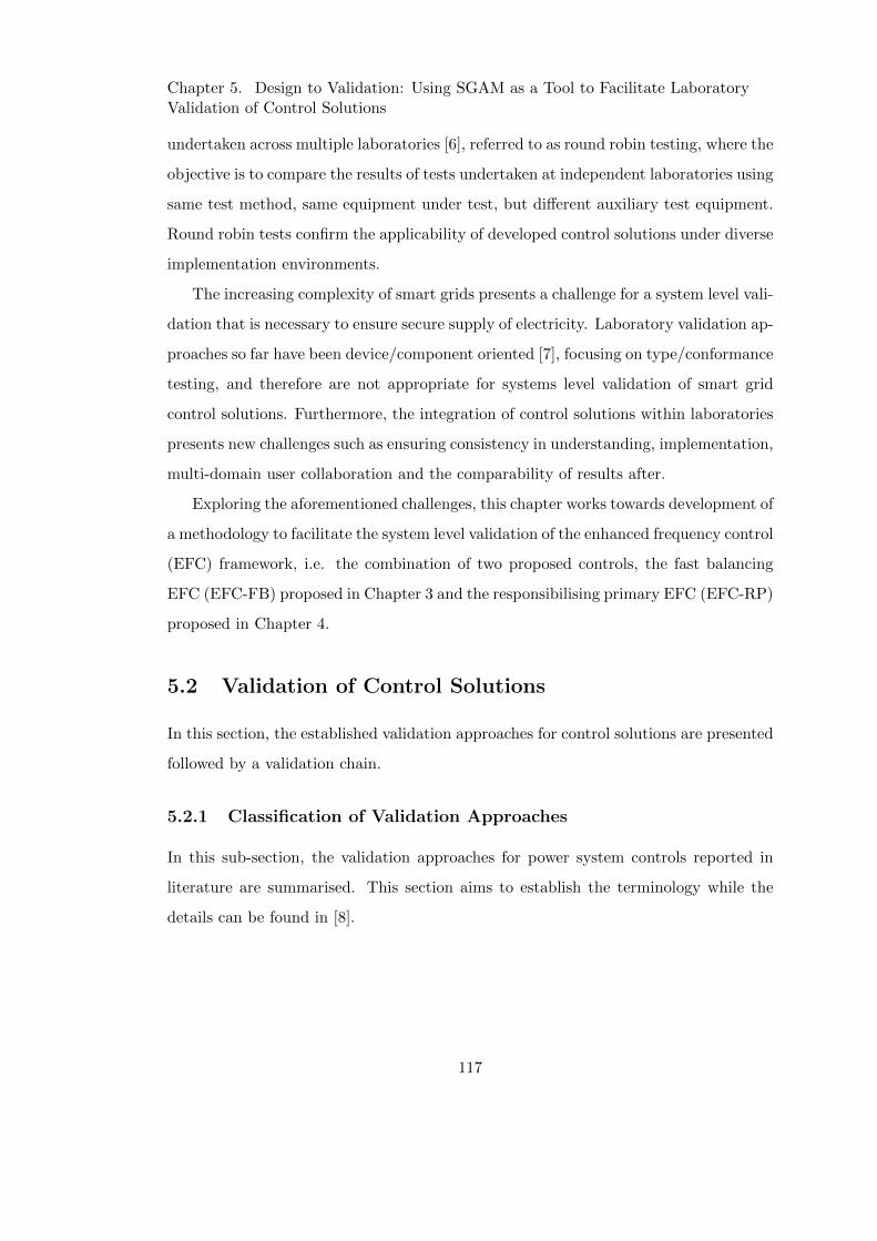
Chapter 5. Design to Validation: Using SGAM as a Tool to Facilitate LaboratoryValidation of Control Solutions
undertaken across multiple laboratories [6], referred to as round robin testing, where the
objective is to compare the results of tests undertaken at independent laboratories using
same test method, same equipment under test, but different auxiliary test equipment.
Round robin tests confirm the applicability of developed control solutions under diverse
implementation environments.
The increasing complexity of smart grids presents a challenge for a system level vali-
dation that is necessary to ensure secure supply of electricity. Laboratory validation ap-
proaches so far have been device/component oriented [7], focusing on type/conformance
testing, and therefore are not appropriate for systems level validation of smart grid
control solutions. Furthermore, the integration of control solutions within laboratories
presents new challenges such as ensuring consistency in understanding, implementation,
multi-domain user collaboration and the comparability of results after.
Exploring the aforementioned challenges, this chapter works towards development of
a methodology to facilitate the system level validation of the enhanced frequency control
(EFC) framework, i.e. the combination of two proposed controls, the fast balancing
EFC (EFC-FB) proposed in Chapter 3 and the responsibilising primary EFC (EFC-RP)
proposed in Chapter 4.
5.2 Validation of Control Solutions
In this section, the established validation approaches for control solutions are presented
followed by a validation chain.
5.2.1 Classification of Validation Approaches
In this sub-section, the validation approaches for power system controls reported in
literature are summarised. This section aims to establish the terminology while the
details can be found in [8].
117

Chapter 5. Design to Validation: Using SGAM as a Tool to Facilitate LaboratoryValidation of Control Solutions
Validation Approaches
Pure Simulation
Offline Simulations
Monolithic
Slower than Real-Time
Faster than Real-Time
Non-Monolithic
Slower than Real-Time
Faster than Real-Time
Real-Time Simulations
Monolithic
Non-Monolithic
Pure Hardware
Controlled Environment
Uncontrolled Environment
Hybrid
C-HiL
P-HiL
Figure 5.1: Classification of validation approaches.
Pure Simulation Approaches
Pure simulation based approaches can be broadly classified into two: (i) off-line simu-
lations and (ii) real-time simulations. To define and distinguish between the two, first
let us define execution time (τex) as the time taken by a processor to integrate given
set of equations for the defined time step (τs). The two types of pure simulations can
now be defined as:
Off-line Simulations: Simulations where τex 6= τs are referred to as off-line simula-
tions.
Real-Time Simulations: Simulations where τex = τs is guaranteed, are referred to
as real-time simulations.
Off-line simulations with τex > τs are referred to as slower than real-time and τex < τs
as faster than real-time. Typically the execution time is always greater than the step
time for off-line simulations. With increase in size and complexity of the system under
simulation, the execution time increases significantly.
118

Chapter 5. Design to Validation: Using SGAM as a Tool to Facilitate LaboratoryValidation of Control Solutions
Pure simulation approaches (both off-line and real-time) can further be classified
into two:
Monolithic: Simulation setup where only one simulation tool is employed.
Non-monolithic: Simulation setup where more than one simulation tool is employed.
Non-monolithic pure simulations can be observed as co-simulation and are also referred
to as software-in-the-loop in literature [9], [10].
Off-line simulations can be considered as the cheapest, easiest, and safest option
available for validation while real-time simulations, with their ability to recreate power
system dynamics at the natural time-scale of their occurrence, are being increasingly
employed to obtain results closer to the real-world.
Pure Hardware Approaches
Validation approach where only actual power system components are utilised is referred
to as pure hardware validation. They can be broadly classified into two depending upon
the environment within which they are undertaken as:
Controlled Environment: Validation undertaken in a controlled environment such
as a laboratory falls under this category. It offers more flexibility in terms of validation
under extreme conditions and is less expensive compared to its alternative.
Uncontrolled Environment: Validation undertaken in the field falls under this cat-
egory, often referred to as field trials. Field trials are expensive and limited to steady-
state validation.
Both the above approaches are undertaken in real-world conditions, offering a higher
degree of confidence. Typically, pure hardware validations are in real-time and often
comprise more than one equipment constituting a real-time non-monolithic setup by
nature.
Hybrid Approaches
Validation approaches that combine simulations and hardware in some form are referred
to as hybrid approaches. They are commonly referred to as Hardware-in-the-Loop (HiL)
simulations, involving a part of the simulated system to be present physically, i.e., as
119
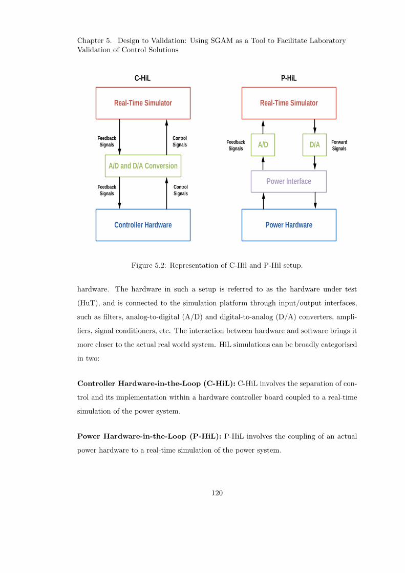
Chapter 5. Design to Validation: Using SGAM as a Tool to Facilitate LaboratoryValidation of Control Solutions
Controller Hardware Power Hardware
A/D and D/A Conversion
A/D
Real-Time Simulator Real-Time Simulator
Control
Signals
Control
Signals
Feedback
Signals
Feedback
Signals
C-HiL P-HiL
D/A
Power Interface
Feedback
Signals
Forward
Signals
Figure 5.2: Representation of C-Hil and P-Hil setup.
hardware. The hardware in such a setup is referred to as the hardware under test
(HuT), and is connected to the simulation platform through input/output interfaces,
such as filters, analog-to-digital (A/D) and digital-to-analog (D/A) converters, ampli-
fiers, signal conditioners, etc. The interaction between hardware and software brings it
more closer to the actual real world system. HiL simulations can be broadly categorised
in two:
Controller Hardware-in-the-Loop (C-HiL): C-HiL involves the separation of con-
trol and its implementation within a hardware controller board coupled to a real-time
simulation of the power system.
Power Hardware-in-the-Loop (P-HiL): P-HiL involves the coupling of an actual
power hardware to a real-time simulation of the power system.
120
Chapter 5. Design to Validation: Using SGAM as a Tool to Facilitate LaboratoryValidation of Control Solutions
Figure 5.3: Validation chain proposed in [5].
The difference essentially lies in the levels (magnitude) of interface signals exchanged
between the hardware and real-time simulation as shown in Fig. 5.2. C-HiL involves
exchange of control signals (usually in the order of±10V) while P-HiL involves exchange
of real power across the interface thus requiring an amplifier as the interface (in addition
to the A/D, D/A cards).
5.2.2 Validation Chain
Having the terminologies of validation approaches established, this sub-section presents
the validation chain for power system controls as proposed in [5], shown in Fig. 5.3.
As can be observed from the figure, the validation chain comprises of five phases.
Phase I: First stage to validation is a pure software simulation approach wherein the
power network and control are developed within one simulation platform. A plethora of
121
Chapter 5. Design to Validation: Using SGAM as a Tool to Facilitate LaboratoryValidation of Control Solutions
commercially available simulation tools can be utilised, some designed for steady state
analysis (for example PSSE [11-13]) and some more specifically for transient analysis
(for example PSCAD [14-16]).
Phase II: To adequately capture the interface between power and control systems, a
natural progression is the use of two dedicated software simulation tools, one for power
system and one for control system in closed loop configuration. In other words, phase
II is a co-simulation or SiL approach [17-19].
Phase III: The next phase involves testing of the control in a C-HiL setup [20-22].
The advantages offered by C-HiL include: (i) the ability to reveal hidden issues of the
control solution (often in terms of its implementation and real-time run capability) and
(ii) allows for control solutions performance to be evaluated under realistic conditions.
Phase IV: The penultimate phase of the validation chain is the combination of C-
HiL and P-HiL techniques in one simulation/experimental setup [23-25]. Such a setup
enables validation of controls under a wide range of scenarios, which can be difficult,
risky, expensive, and even impossible to perform in real life systems.
Phase V: The final phase of validation is by means of its implementation within the
field.
The validation chain presented above is intended to be carried out serially for rigorous
validation of a control solution developed for power systems. It should however be noted
that phase I/II is/are often the only validation undertaken by researchers. This can be
associated to the lack of availability of equipment required for the consequent phases
of validation chain. It is also important to note that each phase of the validation chain
offers significant advances in terms of the readiness of the proposed control solution. To
illustrate this better, consider the relation drawn between each phase of the validation
chain and technology readiness level (TRL) [26] in Fig. 5.4.
Phase I and II effectively establish the feasibility and soundness of the developed
122
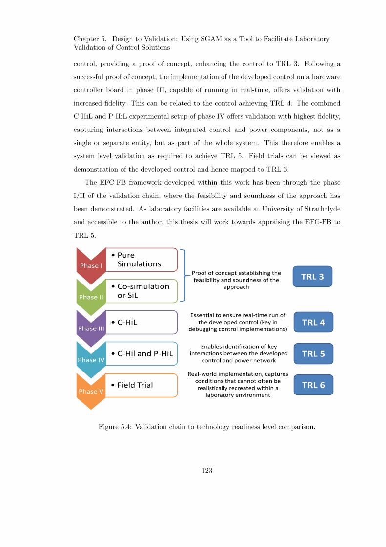
Chapter 5. Design to Validation: Using SGAM as a Tool to Facilitate LaboratoryValidation of Control Solutions
control, providing a proof of concept, enhancing the control to TRL 3. Following a
successful proof of concept, the implementation of the developed control on a hardware
controller board in phase III, capable of running in real-time, offers validation with
increased fidelity. This can be related to the control achieving TRL 4. The combined
C-HiL and P-HiL experimental setup of phase IV offers validation with highest fidelity,
capturing interactions between integrated control and power components, not as a
single or separate entity, but as part of the whole system. This therefore enables a
system level validation as required to achieve TRL 5. Field trials can be viewed as
demonstration of the developed control and hence mapped to TRL 6.
The EFC-FB framework developed within this work has been through the phase
I/II of the validation chain, where the feasibility and soundness of the approach has
been demonstrated. As laboratory facilities are available at University of Strathclyde
and accessible to the author, this thesis will work towards appraising the EFC-FB to
TRL 5.
Phase I
• Pure Simulations
Phase II
• Co-simulation or SiL
Phase III • C-HiL
Phase IV • C-Hil and P-HiL
Phase V • Field Trial
Proof of concept establishing the feasibility and soundness of the
approach
TRL 3
Essential to ensure real-time run of the developed control (key in
debugging control implementations) TRL 4
TRL 5
TRL 6
Enables identification of key interactions between the developed
control and power network
Real-world implementation, captures conditions that cannot often be realistically recreated within a
laboratory environment
Figure 5.4: Validation chain to technology readiness level comparison.
123
Chapter 5. Design to Validation: Using SGAM as a Tool to Facilitate LaboratoryValidation of Control Solutions
5.3 Challenges with Laboratory Validation of Control So-
lutions
Challenges faced by laboratory users can be classified into two: (i) technical challenges
and (ii) practical challenges. Technical challenges are often associated with capabilities
of a laboratory. A good example is the stability and accuracy of a P-HiL setup, where
ensuring a stable and accurate P-HiL setup for experimental validation is challenging
and offers excellent research opportunities that are continuously addressed and reported
by the research community. On the other hand, the practical challenges associated
with laboratory validations have not been given much importance to date, although
they are often time consuming and well recognised as an issue within the laboratory
user community.
With increasing significance of laboratory validations, practical challenges are now
being acknowledged as an important research direction. This section works towards
establishing a set of practical challenges, derived by a discussion between dynamic
power systems laboratory (DPSL) users, in consultation with users of three laboratories
across Europe, and further developed through thought experiments. In addition, this
section aims to deduce the root causes of these challenges.
The practical challenges with laboratory validations can be classified into two cate-
gories:
1. Single laboratory validation challenges
2. Multiple laboratory validation challenges
The following two sub-sections present each category in detail.
5.3.1 Single Laboratory Validation Challenges
Real-Time Implementation
Laboratory validations are expensive and control solution developers visit the labora-
tories for a short duration of time in order to validate their control solutions. As is
usually the case, the control solutions are developed independently of the laboratory
124

Chapter 5. Design to Validation: Using SGAM as a Tool to Facilitate LaboratoryValidation of Control Solutions
within which they will be validated. Furthermore, the control solution developers are
used to monolithic implementation (i.e. within a simulation tool) and do not necessar-
ily understand the real-time requirements of laboratory implementation. The control
solutions developed and brought to the laboratory for their validation by the control
solution developers often require changes to enable the developed control to run in
real-time. These changes may involve minor modifications to the control or sometimes
complete re-development from scratch on a different platform. Therefore, it has been
observed that usually more than one visit is required to carry out validation of control
solutions, where the first visit is spent in understanding the implementation environ-
ment and the required control changes, and the second where the validation takes place.
Multi-Domain User Collaboration
Similar to the evolution of smart grids, the smart grid laboratories are in the process of
continuous evolution and development. This development involves not only the addition
of new equipment but also incorporation of new domains within the laboratories. This
although enhances the capabilities of a laboratory, brings forth challenges in terms of
multi-domain user collaboration. The process of validation of control solutions within a
laboratory is adhoc, and with multiple users and multiple domains, this becomes even
more challenging. Although the adhoc process of validation suits the dynamic nature
of research work undertaken, it is not efficient and may lead to serialisation of tasks.
Repeatability
Generally speaking, users of the laboratories have a particular expertise they develop
over time. The expertise may be (i) domain specific, such as communications, multi-
agent systems, or power systems, (ii) research area specific, such as protection, fre-
quency control or wide area monitoring and control, (iii) kit specific or (iv) technique
specific such as real-time power hardware in the loop. Upon the departure of the users
either due to graduation, or change in position, the transfer of knowledge is not always
an easy process. This leads to uncertainty in terms of repeatability of experiments. Fur-
thermore, when a particular control solution is enhanced after its initial validation and
125
Chapter 5. Design to Validation: Using SGAM as a Tool to Facilitate LaboratoryValidation of Control Solutions
brought for re-validation, not only is repeatability uncertain, often the whole process
of implementing the control from scratch is chosen, i.e. there is little or no provision of
extending the previously done experiments.
5.3.2 Multiple Laboratory Validation/ Round Robin Validation Chal-
lenges
Round robin testing refers to an inter-laboratory test undertaken independently a num-
ber of times. This involves testing by independent laboratories using same method and
same or different equipment. Within power systems domain, round robin tests are
generally undertaken on equipment, where the objective is to compare the results of
tests undertaken at independent laboratories using same test method, same equipment
under test, but different auxiliary test equipment. Development of round robin test
procedures is an active area of research where the objective is to ensure the repro-
ducibility of such procedures and is often undertaken by standardisation bodies [27].
In terms of validation of novel control solutions for smart grids, round robin tests can be
undertaken to ensure the applicability of the developed control solution under diverse
implementation environments. However, contrary to the testing of equipment where
standard testing procedures can be developed, the nature of validation of control so-
lutions is more dynamic. An important aspect to ensure while undertaking multiple
laboratory testing is the comparability of results and the following challenges can be
observed:
Consistency in Implementation
An important aspect to understand is that no two smart grid laboratories are the
same. It is not uncommon that when a control solution is presented to two different
laboratory user groups, the understanding in implementation of the two user group
varies. This difference in understanding might be infrastructure driven or convenience
driven. Most of the smart grid laboratories are designed to be flexible, and there is often
more than one way in which a particular control solution can be implemented, unless
otherwise restricted by infrastructure availability. Therefore, if results of validation
126
Chapter 5. Design to Validation: Using SGAM as a Tool to Facilitate LaboratoryValidation of Control Solutions
carried out independently at two laboratories are to be compared, the consistency in
its implementation needs to be maintained.
Consistency in Recording and Reporting
To elaborate on the differences between two smart grid laboratories, the practices of
recording and reporting experimentation results is a good example. In order for the
results of two laboratories to be compared, consistency in terms of data recording
and reporting needs to be maintained. Although a lot of work in this area is being
undertaken in terms of developing standards such as IEC 61850 [28] and Common
Information Model [29], not all laboratories have these standards incorporated and
much effort is required to do so.
5.3.3 Analysing Laboratory Validation Challenges
Having the challenges associated with laboratory validation described, this sub-section
presents some of the underlying causes deduced.
Limited Laboratory Engagement
It can be said that if laboratory validation of a control solution is the goal, as would be
in the case when appraisal of a proposed control solution to TRL 5 is desired, involving
the laboratory (or laboratory user group) in earlier stages of design and development of
control solution would be beneficial. Consulting with targeted laboratory user groups
during the developmental stages of a control solution can save valuable time.
Laboratory Infrastructure Bias
When control solutions are presented to multiple laboratory user groups, their un-
derstanding of its implementation is biased towards their individual laboratory infras-
tructure. This is not uncommon and is definitely not wrong. However, if the control
solution is presented in a format that would enable the laboratory user groups to un-
ambiguously identify the infrastructure needs to validate the solution, this can lead to
more consistent implementation.
127

Chapter 5. Design to Validation: Using SGAM as a Tool to Facilitate LaboratoryValidation of Control Solutions
Multi-Domain Interoperability
Incorporating more than one domain in laboratory validation, in some simple form,
has existed for a while. For example, communication delay being incorporated within
laboratory validation in the form of a simple delay block (readily available in most
commercial simulation tools). However, laboratories have witnessed inclusion of more
sophisticated, dedicated, domain specific equipments and simulation tools. With these
changes, it is important to develop a multi-domain approach to validation.
Lack of an Integrated Methodology
It is recognised that development of standard procedures for validation of novel control
solutions is difficult owing to the the dynamic nature of validation (different control
solutions would entail different validation objectives and approaches). However, a more
holistic approach to deriving an integrated methodology can be undertaken. The need
for such integrated methodology has also been acknowledged by the European Commis-
sion as is evident from the scope of the ERIGrid project [30]. It can also be inferred that
some of the aforementioned challenges with laboratory validation can be attributed to
lack of an integrated approach to validation.
Therefore, some of the challenges associated with laboratory validation of control solu-
tions can be overcome if an integrated methodology is developed that incorporates the
following features:
• Involves active engagement of laboratory (or laboratory user group) during the
design and development of control solution.
• Defines a common unambiguous template for control solution description.
• Incorporates multiple domains and allows for interoperability to be captured.
• Defines a common template for documenting validation approach undertaken.
Such a methodology would facilitate the transition of control solution from its design to
its validation. The emphasis on consistent implementations across multiple laboratories
128
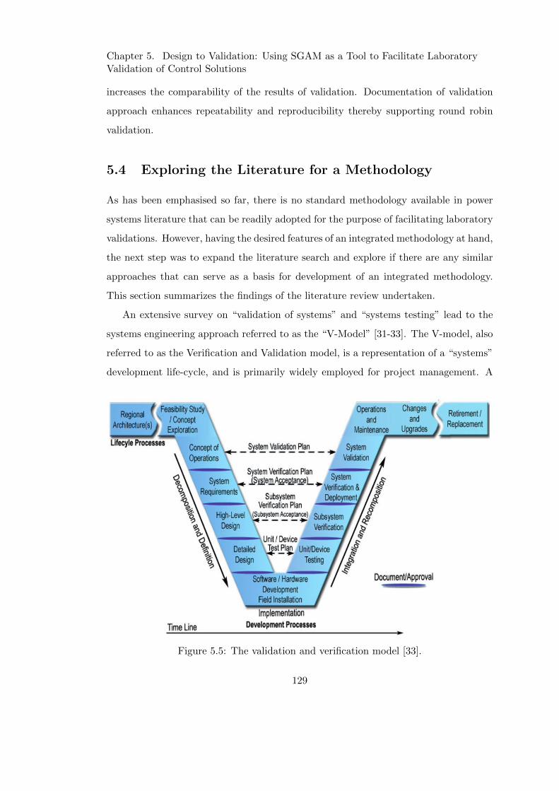
Chapter 5. Design to Validation: Using SGAM as a Tool to Facilitate LaboratoryValidation of Control Solutions
increases the comparability of the results of validation. Documentation of validation
approach enhances repeatability and reproducibility thereby supporting round robin
validation.
5.4 Exploring the Literature for a Methodology
As has been emphasised so far, there is no standard methodology available in power
systems literature that can be readily adopted for the purpose of facilitating laboratory
validations. However, having the desired features of an integrated methodology at hand,
the next step was to expand the literature search and explore if there are any similar
approaches that can serve as a basis for development of an integrated methodology.
This section summarizes the findings of the literature review undertaken.
An extensive survey on “validation of systems” and “systems testing” lead to the
systems engineering approach referred to as the “V-Model” [31-33]. The V-model, also
referred to as the Verification and Validation model, is a representation of a “systems”
development life-cycle, and is primarily widely employed for project management. A
Figure 5.5: The validation and verification model [33].
129
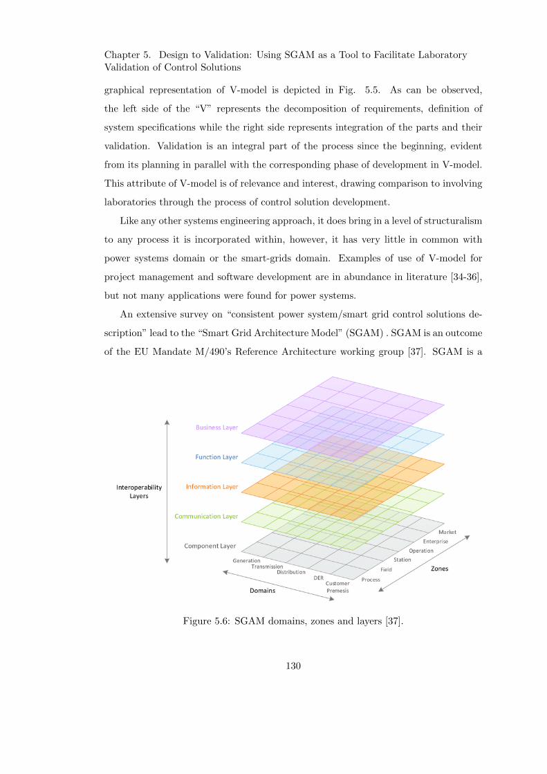
Chapter 5. Design to Validation: Using SGAM as a Tool to Facilitate LaboratoryValidation of Control Solutions
graphical representation of V-model is depicted in Fig. 5.5. As can be observed,
the left side of the “V” represents the decomposition of requirements, definition of
system specifications while the right side represents integration of the parts and their
validation. Validation is an integral part of the process since the beginning, evident
from its planning in parallel with the corresponding phase of development in V-model.
This attribute of V-model is of relevance and interest, drawing comparison to involving
laboratories through the process of control solution development.
Like any other systems engineering approach, it does bring in a level of structuralism
to any process it is incorporated within, however, it has very little in common with
power systems domain or the smart-grids domain. Examples of use of V-model for
project management and software development are in abundance in literature [34-36],
but not many applications were found for power systems.
An extensive survey on “consistent power system/smart grid control solutions de-
scription” lead to the “Smart Grid Architecture Model” (SGAM) . SGAM is an outcome
of the EU Mandate M/490’s Reference Architecture working group [37]. SGAM is a
Figure 5.6: SGAM domains, zones and layers [37].
130
Chapter 5. Design to Validation: Using SGAM as a Tool to Facilitate LaboratoryValidation of Control Solutions
reference model intended to analyse and visualize smart grid use cases in a technology-
neutral manner. It provides a systematic approach to cope with the complexity of smart
grids, allowing representation of control solutions in the current state of the electrical
grid as well as the ability to capture their evolution and integration within future smart
grid scenarios.
The three dimensional representation of SGAM spans six hierarchical power system
zones (Process, Field, Station, Operation, Enterprise and Market) and five domains
encompassing complete electrical energy conversion chain (Generation, Transmission,
Distribution, Distributed Energy Resources and Customer Premise) as shown in Fig.
5.6. Five superimposed layers (Business, Function, Information, Communication and
Component Layer) allow for the interoperability of multiple functions in the power sys-
tem to be depicted. Such a representation enables different smart grid control solutions
to be visualised and compared.
The SGAM combines effective approaches of systems engineering with power sys-
tems in a simple yet comprehensive manner. SGAM builds upon significant existing
work such as the National Institute of Standards and Technology (NIST) Conceptual
Model [38], the GridWise Architecture Council Stack interoperability categories [39],
the IntelliGrid Methodology [40], the European Conceptual Model and architecture
standards like The Open Group Architecture Framework (TOGAF) and Archimate
[41].
The use of SGAM in literature has been limited so far. One of the first reported
use of SGAM was by standardisation bodies to identify standardisation gaps [42]. The
capabilities of SGAM were then further enhanced by development of a methodology
that allowed for smart grid control solutions to be represented within the three dimen-
sions of SGAM (referred to as SGAM mappings henceforth) and analysed [43]. This
was undertaken as part of the DISCERN project [44], where the participating Dis-
tribution System Operators (DSO) produced SGAM mappings for a control solutions
deployed within their network [45]. The SGAM mappings of each DSO were then inde-
pendently analysed by other participating DSOs. The objective was to allow DSOs to
exchange information on smart grid realisation options from their experience of smart
131
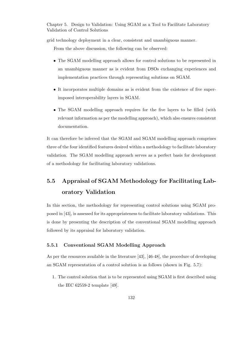
Chapter 5. Design to Validation: Using SGAM as a Tool to Facilitate LaboratoryValidation of Control Solutions
grid technology deployment in a clear, consistent and unambiguous manner.
From the above discussion, the following can be observed:
• The SGAM modelling approach allows for control solutions to be represented in
an unambiguous manner as is evident from DSOs exchanging experiences and
implementation practices through representing solutions on SGAM.
• It incorporates multiple domains as is evident from the existence of five super-
imposed interoperability layers in SGAM.
• The SGAM modelling approach requires for the five layers to be filled (with
relevant information as per the modelling approach), which also ensures consistent
documentation.
It can therefore be inferred that the SGAM and SGAM modelling approach comprises
three of the four identified features desired within a methodology to facilitate laboratory
validation. The SGAM modelling approach serves as a perfect basis for development
of a methodology for facilitating laboratory validations.
5.5 Appraisal of SGAM Methodology for Facilitating Lab-
oratory Validation
In this section, the methodology for representing control solutions using SGAM pro-
posed in [43], is assessed for its appropriateness to facilitate laboratory validations. This
is done by presenting the description of the conventional SGAM modelling approach
followed by its appraisal for laboratory validation.
5.5.1 Conventional SGAM Modelling Approach
As per the resources available in the literature [43], [46-48], the procedure of developing
an SGAM representation of a control solution is as follows (shown in Fig. 5.7):
1. The control solution that is to be represented using SGAM is first described using
the IEC 62559-2 template [49].
132
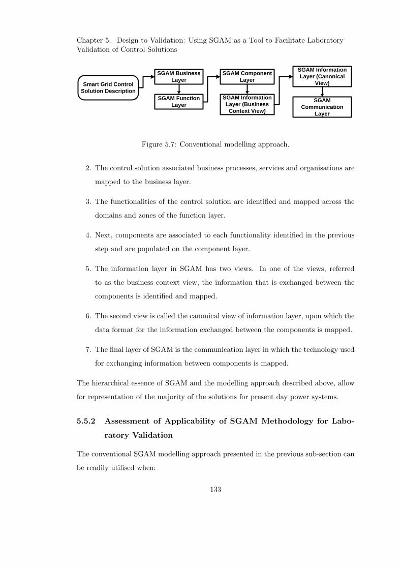
Chapter 5. Design to Validation: Using SGAM as a Tool to Facilitate LaboratoryValidation of Control Solutions
Smart Grid Control
Solution Description
SGAM Business
Layer
SGAM Function
Layer
SGAM Information
Layer (Business
Context View)
SGAM Information
Layer (Canonical
View)
SGAM Component
Layer
SGAM
Communication
Layer
Figure 5.7: Conventional modelling approach.
2. The control solution associated business processes, services and organisations are
mapped to the business layer.
3. The functionalities of the control solution are identified and mapped across the
domains and zones of the function layer.
4. Next, components are associated to each functionality identified in the previous
step and are populated on the component layer.
5. The information layer in SGAM has two views. In one of the views, referred
to as the business context view, the information that is exchanged between the
components is identified and mapped.
6. The second view is called the canonical view of information layer, upon which the
data format for the information exchanged between the components is mapped.
7. The final layer of SGAM is the communication layer in which the technology used
for exchanging information between components is mapped.
The hierarchical essence of SGAM and the modelling approach described above, allow
for representation of the majority of the solutions for present day power systems.
5.5.2 Assessment of Applicability of SGAM Methodology for Labo-
ratory Validation
The conventional SGAM modelling approach presented in the previous sub-section can
be readily utilised when:
133
Chapter 5. Design to Validation: Using SGAM as a Tool to Facilitate LaboratoryValidation of Control Solutions
• Solutions already implemented in the field are to be visualised.
• Novel solutions are to be implemented within the installed utility equipment.
However, for the purpose of laboratory validation of novel control solutions, shortcom-
ings within the conventional SGAM modelling approach have been identified and listed
below:
S1. Missing Validation Objectives: The IEC 62559-2 template is aimed at de-
riving a technical requirement specification for implementation of a control solution in
the field (i.e., within the installed utility equipment). This is not directly of relevance
to laboratory validation. In contrast, for laboratory validation, deriving the objectives
of validation is of more importance.
S2. Redundant Layer: SGAM is multi-faceted, allowing not only for technical
implementation details of control solution to be depicted but also incorporating the
business, organisational and regulatory aspects associated with the control solution.
Although, this depiction within the business layer of SGAM does have an practical
relevance to DSOs, it is not of relevance for laboratory validation of any given control
solution.
S3. Inadequate Sequence of Layer Mapping: Within the conventional approach,
after functionalities of a control solution are identified, the next step is to identify
components that can be associated to the functionalities. As mentioned earlier, this
is practical for control solutions that are already implemented within the field, or
when a control solution has to be implemented within a given set of utility equipment.
However, this transition from function layer to component layer is not appropriate
for laboratory validation. Consider the following example: a simple control function,
moving average filter, is to be implemented within laboratory. Within the DPSL, there
are five implementation platforms (equipment) that can be utilised for this purpose.
Without any additional information, the choice of equipment would be based on ease
of implementation. However, this might not be an appropriate choice. On the other
134
Chapter 5. Design to Validation: Using SGAM as a Tool to Facilitate LaboratoryValidation of Control Solutions
hand, if the information that the control function is required to exchange is known, the
frequency of information exchange is known, a more informed decision on the choice of
implementation platform can be made.
S4. No Demarcation of Responsibility: The present methodology does not ex-
plicitly demarcate the responsibilities of the control solution developers and the labo-
ratory users, although the involvement of the two is implicit.
S5. Unambiguous Guidance on Zone Mapping: The mapping of a function to
an SGAM domain and zone is an integral step of the SGAM modelling approach. There
is no formal guidance available on how a function is to be mapped on to a corresponding
domain and zone. The formal description of the SGAM domains and zones, in addition
to a limited number of example mappings in literature, serve as the only guidelines
for prospective SGAM users. When novel control solutions are to be mapped on to
SGAM, these guidelines may not be directly applicable. For a given control function,
it is quite clear to which domain (generation, transmission, distribution, distributed
energy resource (DER) or customer) it belongs to, however the description of zones is
ambiguous and generally leads to users choosing a zone based on their understanding.
As the objective of utilising SGAM is consistency, a clear set of unambiguous guidelines
to choose a zone for control function are required.
S6. Limited to Representation of Control Solutions within a Single Entity:
Due to the hierarchical nature of SGAM, solutions that can be represented using SGAM
correspond to one single entity, such as a Transmission System Operator (TSO) or a
Distribution Network Operator (DNO). If a control solution involves two TSOs, two
SGAM representations are required, one for each TSO.
Therefore, the conventional SGAM methodology, presented in this section, requires
adaptation to enable its effective utilisation to facilitate the laboratory validation of
novel control solutions.
135

Chapter 5. Design to Validation: Using SGAM as a Tool to Facilitate LaboratoryValidation of Control Solutions
5.6 Proposed SGAM Modelling Approach for Laboratory
Validation
In this section, the shortfalls identified within the conventional SGAM modelling ap-
proach will be addressed. First, an adapted SGAM modelling approach is proposed,
followed by formalisation of guidelines for mapping functions on zones of SGAM plane.
5.6.1 Adapted SGAM Modelling Approach
The proposed SGAM modelling approach is presented in Fig. 5.8. As can be seen
from the figure, the modelling approach is structured in four stages. The following
subsections will present each of the stages in detail.
Stage I: Control Solution Description
For control solutions to be validated within a laboratory, it is essential to formulate
clear validation objectives. In the conventional modelling procedure, the use case is
described using the IEC 62559 template. However, as the IEC 62559 template is not
intended to be utilised for the purpose of laboratory validation, a template specific
to laboratory testing should be utilised, such as that presented in [50]. The test case
specification template of [50] aims to clarify the “why, what and how” of the validation
that is intended to be carried out. The template comprises a narrative, identification
SGAM Component
Layer
Smart Grid Control
Solution
Description
Reference
Power System
Laboratory
Infrastructure
Stage I Stage II Stage III Stage IV
SGAM Function
Layer
SGAM Information
Layer (Business
Context View)
SGAM
Communication
Layer
SGAM Information
Layer (Canonical
View)
Figure 5.8: Modelling approach for laboratory validation.
136
Chapter 5. Design to Validation: Using SGAM as a Tool to Facilitate LaboratoryValidation of Control Solutions
of functions under test (FuT), establishing the purpose of investigation (PoI) and the
test criteria (TCR). The narrative is a storyline summarising the motivation and scope
of the test to be undertaken, FuT is a list of all functions required for the test. PoI
formulates purpose of test in terms of characterisation, verification or validation while
TCR enlists the measures to be quantified and evaluated for each PoI. This effectively
addresses the shortcoming S1.
Stage II: Consolidated Function Mapping
As the business processes, services and organisations are not of interest for labora-
tory validation, the business layer can be omitted from the process. Similar to the
conventional process, once the use case is described using the test case specification,
the functions identified are mapped on to the function layer. However, after defin-
ing the function layer, in contrast to the conventional process, the information that is
exchanged between the different functions is identified and the business context view
of the SGAM information layer is developed. The next step is to establish the data
transfer requirements (e.g. periodic refresh rate) for the information that is exchanged
between the functions. This depends upon the application of the control solution and
is usually determined by the control solution developers. The population of functional
layer and the business context view of information layer completes the second stage of
the methodology. The omission of business layer from the modelling process and the
transition from function layer to business context view of information layer addresses
the shortcomings S2 and S3. The process until now, stages I and II, is to be carried
out by the control developers who wish for their developed solution to be tested within
a laboratory.
Stage III: Reference Power System Selection
The remainder of the modelling process is to be undertaken by the laboratory that
is to carry out the intended validation. In order to test and validate the smart grid
control solution in the laboratory, a reference power network is required. In most
laboratories, the reference power network is the power network available within the
137
Chapter 5. Design to Validation: Using SGAM as a Tool to Facilitate LaboratoryValidation of Control Solutions
laboratory. However, in laboratories capable of conducting power hardware-in-the-loop
simulations (P-HiL), a larger power network can be simulated, with the laboratory
network being a small part of the larger virtually simulated network. In such cases,
a reference power system is chosen based on the individual laboratory capabilities.
Furthermore, the objectives of the validation also influence the choice of reference
power network. The clear assignment of responsibility to control solution developers
and laboratory users and the a clear demarcation in the process addresses shortcoming
S4.
Stage IV: Experiment Specification
Depending upon the data transfer requirements established in Stage II, the components
– i.e. the intelligent electronic devices (IEDs) – in the laboratory that can be utilised
for the implementation of the functions are identified. Once the components have been
identified, the communication protocols and data formats supported by these compo-
nents are summarised in a table. This enables the population of the component layer,
communication layer and canonical view of information layer of SGAM. Having all the
layers of SGAM populated provides a full view of the laboratory testing environment.
5.6.2 SGAM Zone Mapping Guidelines
In this section, guidelines for the zone mapping of a control solution functions are
established by means of presenting the formal descriptions of zones and contrasting the
changes and enhancements required, thereby addressing shortfall S5.
Process Zone
Definition: This zone is utilised to represent physical, chemical or spatial transfor-
mation of energy (such as power generation itself) and any equipment involved (such
as generator).
Remark 1: From the above description, it is clear that the process zone involves the
elementary devices of the power system
138
Chapter 5. Design to Validation: Using SGAM as a Tool to Facilitate LaboratoryValidation of Control Solutions
Guideline 1: For the purpose of representation of control solution functions, the
process zone is not utilised. However, physical power system components expected to
be part of the validation are represented on the process zone.
Field Zone
Definition: Any equipment to protect, control and monitor the process of power sys-
tem is attributed to the field zone. Examples include protection relays, bay controllers
and any IED that acquires data from power system.
Remark 2: The formal description of field zone refers to equipment only, although
it might be intuitive to map control functions associated with such equipment, it may
constitute to confusion.
Guideline 2: Any control function that is implemented at a device level is attributed
to the field zone. Examples of such controls include speed governing control of syn-
chronous machines and local power controller of domestic heater.
Station Zone
Definition: Aggregation of field zone functions or equipment are represented on the
station zone. Data concentrators, substation automation and SCADA systems are some
examples presented in literature.
Guideline 3: Any control function that operates at an aggregated level is attributed
to station zone. This includes any function that relies on aggregated data or controls
an aggregation of devices. Demand side aggregators form a good example of functions
to be mapped on to the station zone.
Operation Zone
Definition: This zone hosts power system control operations. This includes distri-
bution management systems, micro-grid management systems, etc.
139
Chapter 5. Design to Validation: Using SGAM as a Tool to Facilitate LaboratoryValidation of Control Solutions
Remark 3: From the above description of operation zone, it may appear that all con-
trol operations of the power system are to be attributed to the operation zone. However,
as is evident, the guidelines being proposed in this work have already attributed control
functions to field and station zone of SGAM. This is another reason why a clear set of
guidelines for consistent SGAM modelling is required.
Guideline 4: A control function that is unique within the entity being represented
on SGAM should be attributed to the operation zone. The word unique here points to
the uniqueness of the objective of the function. If only one function with a particular
objective exists, it should be represented on the operation zone. If more than one
control function with a similar objective might exist, such control functions should be
attributed to the station zone.
Enterprise Zone
Definition: Includes commercial and organisational processes, services and infras-
tructures for enterprises. Examples are asset management, logistics, staff training etc.
Remark 4: The description of enterprise zone renders it irrelevant for laboratory
validation of novel control solutions. However, as has been mentioned earlier, only a
control solution implemented within an entity can be represented using SGAM. If a
control solution within an entity relies on information exchange from another entity,
there is no guidance available on how this interaction can be captured.
Guideline 5: Any control function within an entity that relies on information from
another entity is attributed to the enterprise zone.
Remark 5: Being able to capture the interaction between two entities renders the
capability of representing distributed control solutions that are implemented at different
entity levels thereby addressing shortfall S6.
140
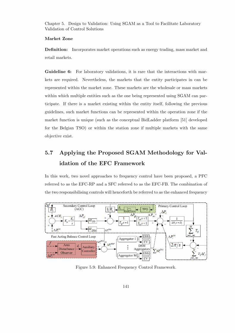
Chapter 5. Design to Validation: Using SGAM as a Tool to Facilitate LaboratoryValidation of Control Solutions
Market Zone
Definition: Incorporates market operations such as energy trading, mass market and
retail markets.
Guideline 6: For laboratory validations, it is rare that the interactions with mar-
kets are required. Nevertheless, the markets that the entity participates in can be
represented within the market zone. These markets are the wholesale or mass markets
within which multiple entities such as the one being represented using SGAM can par-
ticipate. If there is a market existing within the entity itself, following the previous
guidelines, such market functions can be represented within the operation zone if the
market function is unique (such as the conceptual BidLadder platform [51] developed
for the Belgian TSO) or within the station zone if multiple markets with the same
objective exist.
5.7 Applying the Proposed SGAM Methodology for Val-
idation of the EFC Framework
In this work, two novel approaches to frequency control have been proposed, a PFC
referred to as the EFC-RP and a SFC referred to as the EFC-FB. The combination of
the two responsibilising controls will henceforth be referred to as the enhanced frequency
Figure 5.9: Enhanced Frequency Control Framework.
141
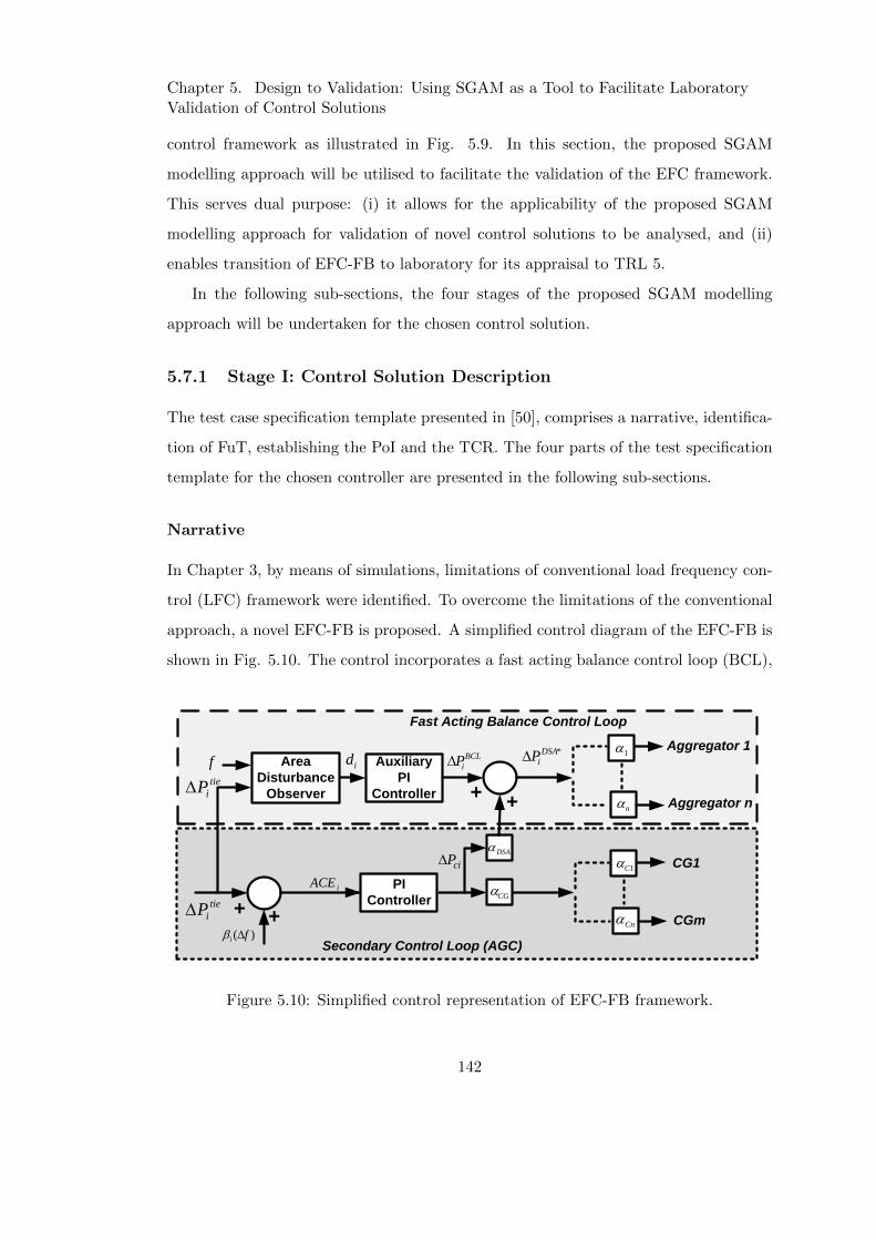
Chapter 5. Design to Validation: Using SGAM as a Tool to Facilitate LaboratoryValidation of Control Solutions
control framework as illustrated in Fig. 5.9. In this section, the proposed SGAM
modelling approach will be utilised to facilitate the validation of the EFC framework.
This serves dual purpose: (i) it allows for the applicability of the proposed SGAM
modelling approach for validation of novel control solutions to be analysed, and (ii)
enables transition of EFC-FB to laboratory for its appraisal to TRL 5.
In the following sub-sections, the four stages of the proposed SGAM modelling
approach will be undertaken for the chosen control solution.
5.7.1 Stage I: Control Solution Description
The test case specification template presented in [50], comprises a narrative, identifica-
tion of FuT, establishing the PoI and the TCR. The four parts of the test specification
template for the chosen controller are presented in the following sub-sections.
Narrative
In Chapter 3, by means of simulations, limitations of conventional load frequency con-
trol (LFC) framework were identified. To overcome the limitations of the conventional
approach, a novel EFC-FB is proposed. A simplified control diagram of the EFC-FB is
shown in Fig. 5.10. The control incorporates a fast acting balance control loop (BCL),
+
PI
Controller
Auxiliary
PI
Controller
Aggregator 1
Aggregator n
CG1
CGm+
Area
Disturbance
Observer
Secondary Control Loop (AGC)
Fast Acting Balance Control Loop
tie
iP
BCL
iP
ciPDSA
CG
*DSA
iP 1
n
1C
Cn)( fi
iACE
tie
iP
f id
++
Figure 5.10: Simplified control representation of EFC-FB framework.
142
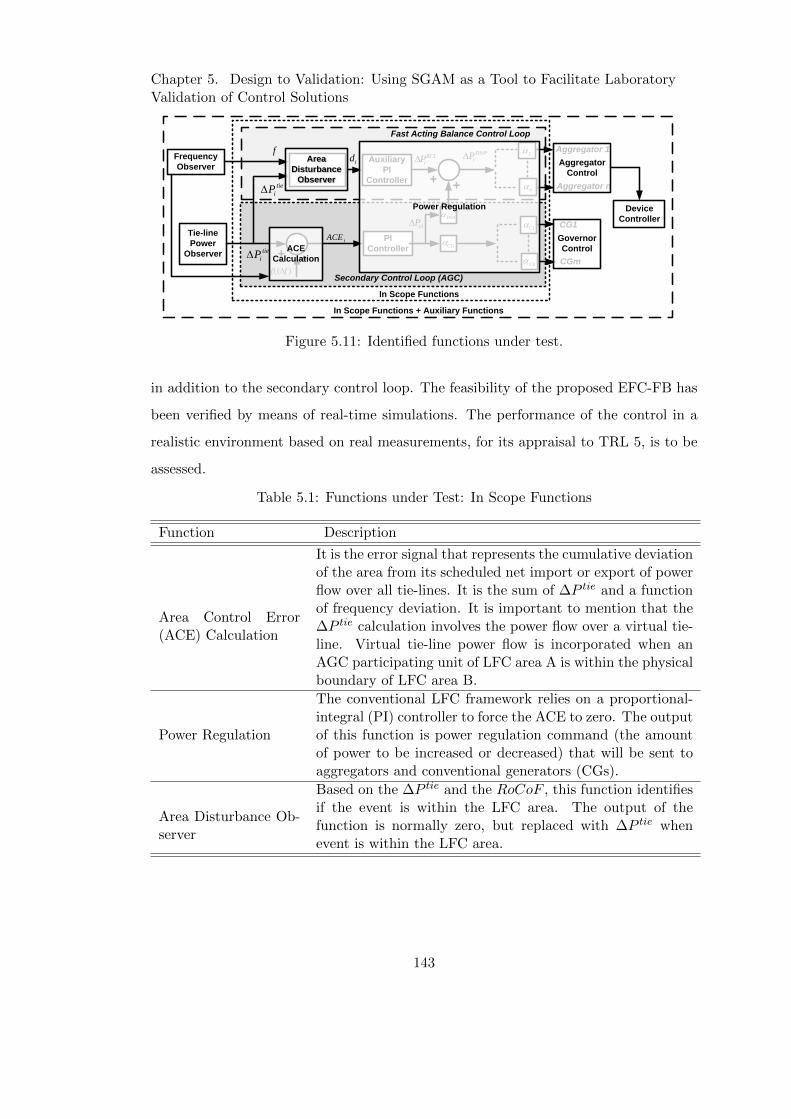
Chapter 5. Design to Validation: Using SGAM as a Tool to Facilitate LaboratoryValidation of Control Solutions
Tie-line
Power
Observer
Frequency
Observer
Device
Controller
In Scope Functions + Auxiliary Functions
+
PI
Controller
Auxiliary
PI
Controller
Aggregator 1
Aggregator n
CG1
CGm+
Area
Disturbance
Observer
Secondary Control Loop (AGC)
Fast Acting Balance Control Loop
tie
iP
BCL
iP
ciPDSA
CG
*DSA
iP 1
n
1C
Cn)( fi
iACE
tie
iP
fid
++
Area
Disturbance
Observer
Power Regulation
Aggregator
Control
Governor
Control
In Scope Functions
ACE
Calculation
Figure 5.11: Identified functions under test.
in addition to the secondary control loop. The feasibility of the proposed EFC-FB has
been verified by means of real-time simulations. The performance of the control in a
realistic environment based on real measurements, for its appraisal to TRL 5, is to be
assessed.
Table 5.1: Functions under Test: In Scope Functions
Function Description
Area Control Error(ACE) Calculation
It is the error signal that represents the cumulative deviationof the area from its scheduled net import or export of powerflow over all tie-lines. It is the sum of ∆P tie and a functionof frequency deviation. It is important to mention that the∆P tie calculation involves the power flow over a virtual tie-line. Virtual tie-line power flow is incorporated when anAGC participating unit of LFC area A is within the physicalboundary of LFC area B.
Power Regulation
The conventional LFC framework relies on a proportional-integral (PI) controller to force the ACE to zero. The outputof this function is power regulation command (the amountof power to be increased or decreased) that will be sent toaggregators and conventional generators (CGs).
Area Disturbance Ob-server
Based on the ∆P tie and the RoCoF , this function identifiesif the event is within the LFC area. The output of thefunction is normally zero, but replaced with ∆P tie whenevent is within the LFC area.
143
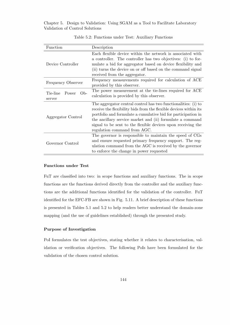
Chapter 5. Design to Validation: Using SGAM as a Tool to Facilitate LaboratoryValidation of Control Solutions
Table 5.2: Functions under Test: Auxiliary Functions
Function Description
Device Controller
Each flexible device within the network is associated witha controller. The controller has two objectives: (i) to for-mulate a bid for aggregator based on device flexibility and(ii) turns the device on or off based on the command signalreceived from the aggregator.
Frequency ObserverFrequency measurements required for calculation of ACEprovided by this observer.
Tie-line Power Ob-server
The power measurement at the tie-lines required for ACEcalculation is provided by this observer.
Aggregator Control
The aggregator central control has two functionalities: (i) toreceive the flexibility bids from the flexible devices within itsportfolio and formulate a cumulative bid for participation inthe ancillary service market and (ii) formulate a commandsignal to be sent to the flexible devices upon receiving theregulation command from AGC.
Governor Control
The governor is responsible to maintain the speed of CGsand ensure requested primary frequency support. The reg-ulation command from the AGC is received by the governorto enforce the change in power requested
Functions under Test
FuT are classified into two: in scope functions and auxiliary functions. The in scope
functions are the functions derived directly from the controller and the auxiliary func-
tions are the additional functions identified for the validation of the controller. FuT
identified for the EFC-FB are shown in Fig. 5.11. A brief description of these functions
is presented in Tables 5.1 and 5.2 to help readers better understand the domain-zone
mapping (and the use of guidelines established) through the presented study.
Purpose of Investigation
PoI formulates the test objectives, stating whether it relates to characterisation, val-
idation or verification objectives. The following PoIs have been formulated for the
validation of the chosen control solution.
144
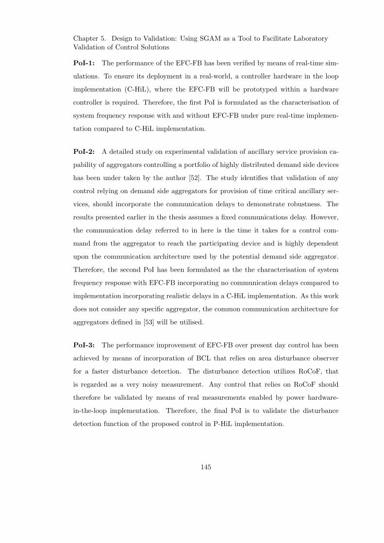
Chapter 5. Design to Validation: Using SGAM as a Tool to Facilitate LaboratoryValidation of Control Solutions
PoI-1: The performance of the EFC-FB has been verified by means of real-time sim-
ulations. To ensure its deployment in a real-world, a controller hardware in the loop
implementation (C-HiL), where the EFC-FB will be prototyped within a hardware
controller is required. Therefore, the first PoI is formulated as the characterisation of
system frequency response with and without EFC-FB under pure real-time implemen-
tation compared to C-HiL implementation.
PoI-2: A detailed study on experimental validation of ancillary service provision ca-
pability of aggregators controlling a portfolio of highly distributed demand side devices
has been under taken by the author [52]. The study identifies that validation of any
control relying on demand side aggregators for provision of time critical ancillary ser-
vices, should incorporate the communication delays to demonstrate robustness. The
results presented earlier in the thesis assumes a fixed communications delay. However,
the communication delay referred to in here is the time it takes for a control com-
mand from the aggregator to reach the participating device and is highly dependent
upon the communication architecture used by the potential demand side aggregator.
Therefore, the second PoI has been formulated as the the characterisation of system
frequency response with EFC-FB incorporating no communication delays compared to
implementation incorporating realistic delays in a C-HiL implementation. As this work
does not consider any specific aggregator, the common communication architecture for
aggregators defined in [53] will be utilised.
PoI-3: The performance improvement of EFC-FB over present day control has been
achieved by means of incorporation of BCL that relies on area disturbance observer
for a faster disturbance detection. The disturbance detection utilizes RoCoF, that
is regarded as a very noisy measurement. Any control that relies on RoCoF should
therefore be validated by means of real measurements enabled by power hardware-
in-the-loop implementation. Therefore, the final PoI is to validate the disturbance
detection function of the proposed control in P-HiL implementation.
145
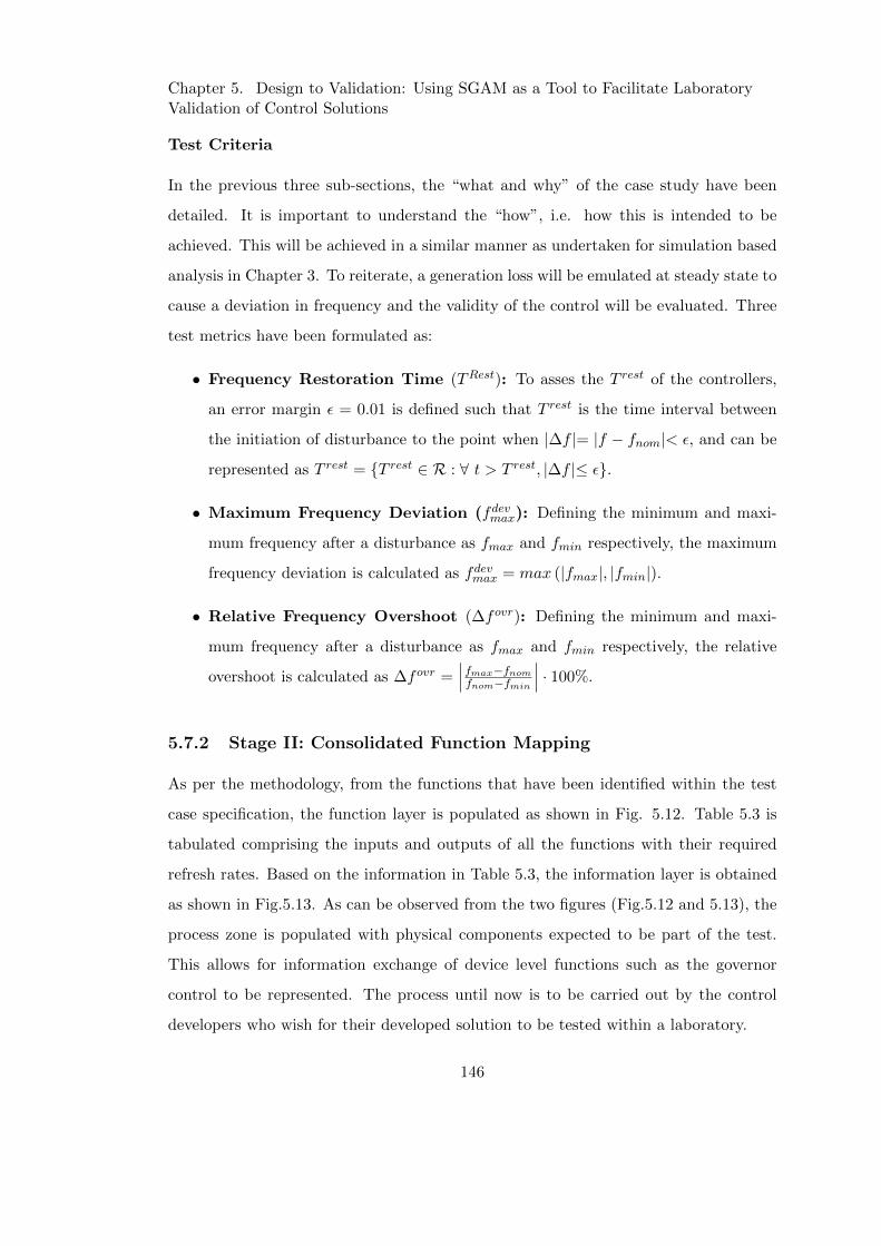
Chapter 5. Design to Validation: Using SGAM as a Tool to Facilitate LaboratoryValidation of Control Solutions
Test Criteria
In the previous three sub-sections, the “what and why” of the case study have been
detailed. It is important to understand the “how”, i.e. how this is intended to be
achieved. This will be achieved in a similar manner as undertaken for simulation based
analysis in Chapter 3. To reiterate, a generation loss will be emulated at steady state to
cause a deviation in frequency and the validity of the control will be evaluated. Three
test metrics have been formulated as:
• Frequency Restoration Time (TRest): To asses the T rest of the controllers,
an error margin ε = 0.01 is defined such that T rest is the time interval between
the initiation of disturbance to the point when |∆f |= |f − fnom|< ε, and can be
represented as T rest = {T rest ∈ R : ∀ t > T rest, |∆f |≤ ε}.
• Maximum Frequency Deviation (fdevmax): Defining the minimum and maxi-
mum frequency after a disturbance as fmax and fmin respectively, the maximum
frequency deviation is calculated as fdevmax = max (|fmax|, |fmin|).
• Relative Frequency Overshoot (∆fovr): Defining the minimum and maxi-
mum frequency after a disturbance as fmax and fmin respectively, the relative
overshoot is calculated as ∆fovr =∣∣∣fmax−fnomfnom−fmin
∣∣∣ · 100%.
5.7.2 Stage II: Consolidated Function Mapping
As per the methodology, from the functions that have been identified within the test
case specification, the function layer is populated as shown in Fig. 5.12. Table 5.3 is
tabulated comprising the inputs and outputs of all the functions with their required
refresh rates. Based on the information in Table 5.3, the information layer is obtained
as shown in Fig.5.13. As can be observed from the two figures (Fig.5.12 and 5.13), the
process zone is populated with physical components expected to be part of the test.
This allows for information exchange of device level functions such as the governor
control to be represented. The process until now is to be carried out by the control
developers who wish for their developed solution to be tested within a laboratory.
146

Chapter 5. Design to Validation: Using SGAM as a Tool to Facilitate LaboratoryValidation of Control Solutions
Table 5.3: Inputs, outputs for FuT with their required refresh rate
Function Inputs(In)
In RefreshRate
Outputs(Out)
Out RefreshRate
ACE CalculationP tiemeas 100 Hz ACEi 100 Hzf 100 HzP tievirtual 100 Hz ∆P tiei 100 Hz
Power RegulationACEi 100 Hz αCG∆Pci 1 Hz∆P tiei 100 Hz ∆PDSA∗i 1 Hz
ADO∆P tiei 100 Hz
∆P tiei 100 Hzf 100 Hz
Aggregator Control δP rDSM 1 Hz ActivationSignal
1 Hz
Device Controller ActivationSignal
1 Hz On/Off 1 Hz
Governor Control αCG∆Pci 1 Hz PSP Continuous
Frequency Observer Raw Mea-surement
Analog Frequency 100 Hz
Tie-line Power Observer Raw Mea-surement
Analog P T iemeas 100 Hz
Aggregator Control
ACE
Calculation
Tie-Line
Power
Observer
ADO
Distribution DER Customer
Pro
ce
ss
Fie
ldS
tatio
nO
pe
ratio
nE
nte
rpris
e
Power
Regulation
Device Controller
Market Zone
Frequency
Observer
Governor
Control
TransmissionGeneration
GeneratorDistribution
Equipment Controllable DevicesTransmission Lines
Figure 5.12: SGAM function layer.
147
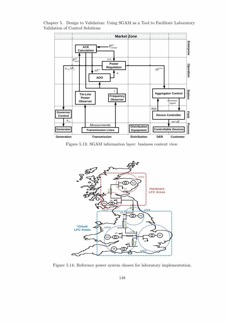
Chapter 5. Design to Validation: Using SGAM as a Tool to Facilitate LaboratoryValidation of Control Solutions
Aggregator Control
ACE
Calculation
Tie-Line
Power
Observer
ADO
Distribution DER Customer
Pro
ce
ss
Fie
ldS
tatio
nO
pe
ratio
nE
nte
rpris
e
Power
Regulation
Device Controller
Market Zone
Frequency
Observer
Governor
Control
TransmissionGeneration
GeneratorDistribution
Equipment Controllable DevicesTransmission Lines
id
tie
iP
iACE
f
*DSA
iP
tie
measP
tie
virtualP
Bids
ActivationSignal
SPP offon/
tsMeasuremen
ciCG P
Figure 5.13: SGAM information layer: business context view.
5
G1
G2
G3
G6
G5G4
L1
L2
L3
L4
L6
L5
LFC1
LFC2 LFC3
LFC4
LFC5
Hardware
LFC Areas
Virtual
LFC Areas
Figure 5.14: Reference power system chosen for laboratory implementation.
148
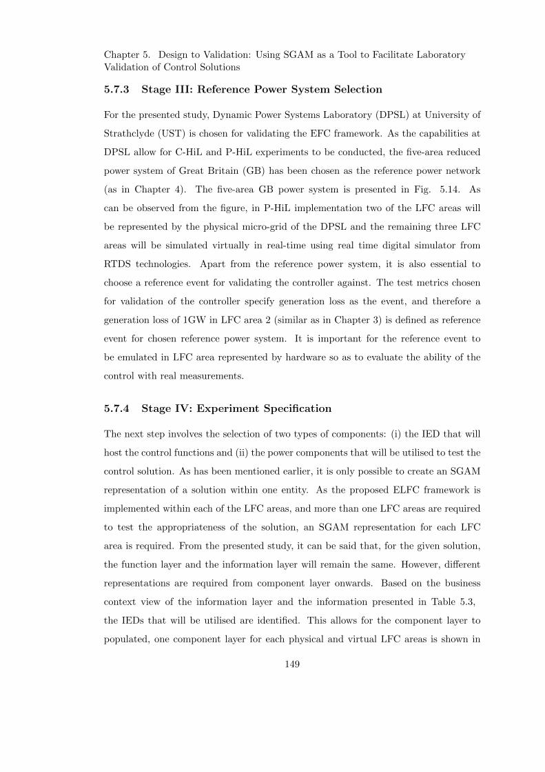
Chapter 5. Design to Validation: Using SGAM as a Tool to Facilitate LaboratoryValidation of Control Solutions
5.7.3 Stage III: Reference Power System Selection
For the presented study, Dynamic Power Systems Laboratory (DPSL) at University of
Strathclyde (UST) is chosen for validating the EFC framework. As the capabilities at
DPSL allow for C-HiL and P-HiL experiments to be conducted, the five-area reduced
power system of Great Britain (GB) has been chosen as the reference power network
(as in Chapter 4). The five-area GB power system is presented in Fig. 5.14. As
can be observed from the figure, in P-HiL implementation two of the LFC areas will
be represented by the physical micro-grid of the DPSL and the remaining three LFC
areas will be simulated virtually in real-time using real time digital simulator from
RTDS technologies. Apart from the reference power system, it is also essential to
choose a reference event for validating the controller against. The test metrics chosen
for validation of the controller specify generation loss as the event, and therefore a
generation loss of 1GW in LFC area 2 (similar as in Chapter 3) is defined as reference
event for chosen reference power system. It is important for the reference event to
be emulated in LFC area represented by hardware so as to evaluate the ability of the
control with real measurements.
5.7.4 Stage IV: Experiment Specification
The next step involves the selection of two types of components: (i) the IED that will
host the control functions and (ii) the power components that will be utilised to test the
control solution. As has been mentioned earlier, it is only possible to create an SGAM
representation of a solution within one entity. As the proposed ELFC framework is
implemented within each of the LFC areas, and more than one LFC areas are required
to test the appropriateness of the solution, an SGAM representation for each LFC
area is required. From the presented study, it can be said that, for the given solution,
the function layer and the information layer will remain the same. However, different
representations are required from component layer onwards. Based on the business
context view of the information layer and the information presented in Table 5.3,
the IEDs that will be utilised are identified. This allows for the component layer to
populated, one component layer for each physical and virtual LFC areas is shown in
149
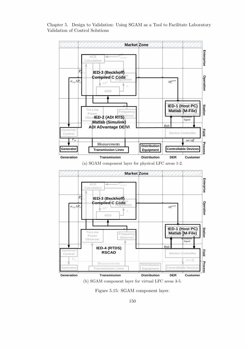
Chapter 5. Design to Validation: Using SGAM as a Tool to Facilitate LaboratoryValidation of Control Solutions
Aggregator Control
ACE
Calculation
Tie-Line
Power
Observer
ADO
Distribution DER Customer
Pro
ce
ss
Fie
ldS
tatio
nO
pe
ratio
nE
nte
rpris
e
Power
Regulation
Device Controller
Market Zone
Frequency
Observer
Governor
Control
TransmissionGeneration
GeneratorDistribution
Equipment Controllable DevicesTransmission Lines
id
tie
iP
iACE
f
*DSA
iP
tie
measP
tie
virtualP
Bids
ActivationSignal
SPP offon/
tsMeasuremen
IED-3 (Beckhoff)
Compiled C Code
IED-1 (Host PC)
Matlab (M-File)
IED-2 (ADI RTS)
Matlab (Simulink)
ADI ADvantage DE/VI
ciCG P
(a) SGAM component layer for physical LFC areas 1-2.
Aggregator Control
ACE
Calculation
Tie-Line
Power
Observer
ADO
Distribution DER Customer
Pro
ce
ss
Fie
ldS
tatio
nO
pe
ratio
nE
nte
rpris
e
Power
Regulation
Device Controller
Market Zone
Frequency
Observer
Governor
Control
TransmissionGeneration
GeneratorDistribution
Equipment Controllable DevicesTransmission Lines
id
tie
iP
iACE
f
*DSA
iP
tie
measP
tie
virtualP
Bids
ActivationSignal
SPP offon/
tsMeasuremen
IED-3 (Beckhoff)
Compiled C Code
IED-1 (Host PC)
Matlab (M-File)
ciCG P
IED-4 (RTDS)
RSCAD
(b) SGAM component layer for virtual LFC areas 3-5.
Figure 5.15: SGAM component layer.
150
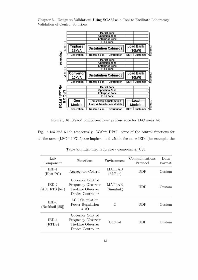
Chapter 5. Design to Validation: Using SGAM as a Tool to Facilitate LaboratoryValidation of Control Solutions
Market Zone
Enterprise ZoneOperation Zone
Field Zone
Pro
ce
ss
Generation Transmission Distribution DER Customer
Controllable
DevicesDistribution Equipment
Load Bank
(10kW)Distribution Cabinet 2
LF
C 1P
hy
sic
al
Triphase
15kVA
Market Zone
Enterprise ZoneOperation Zone
Field Zone
Pro
ce
ss
Generation Transmission Distribution DER Customer
Controllable
DevicesDistribution Equipment
Load Bank
(10kW)Distribution Cabinet 3
LF
C 2 Convertor
10kVA
Market Zone
Enterprise ZoneOperation Zone
Field Zone
Pro
ce
ss
Generation Transmission Distribution DER Customer
Controllable
DevicesDistribution Equipment
Load
ModelsTransmission, Distribution
Lines & Transformer Models
Gen
Models
LF
C 3
-5
Virtu
al : R
TD
S
Figure 5.16: SGAM component layer process zone for LFC areas 1-6.
Fig. 5.15a and 5.15b respectively. Within DPSL, some of the control functions for
all the areas (LFC 1-LFC 5) are implemented within the same IEDs (for example, the
Table 5.4: Identified laboratory components: UST
LabComponent
Functions EnvironmentCommunications
ProtocolData
Format
IED-1(Host PC)
Aggregator ControlMATLAB(M-File)
UDP Custom
IED-2(ADI RTS [54])
Governor ControlFrequency ObserverTie-Line ObserverDevice Controller
MATLAB(Simulink)
UDP Custom
IED-3(Beckhoff [55])
ACE CalculationPower Regulation
ADOC UDP Custom
IED-4(RTDS)
Governor ControlFrequency ObserverTie-Line ObserverDevice Controller
Control UDP Custom
151
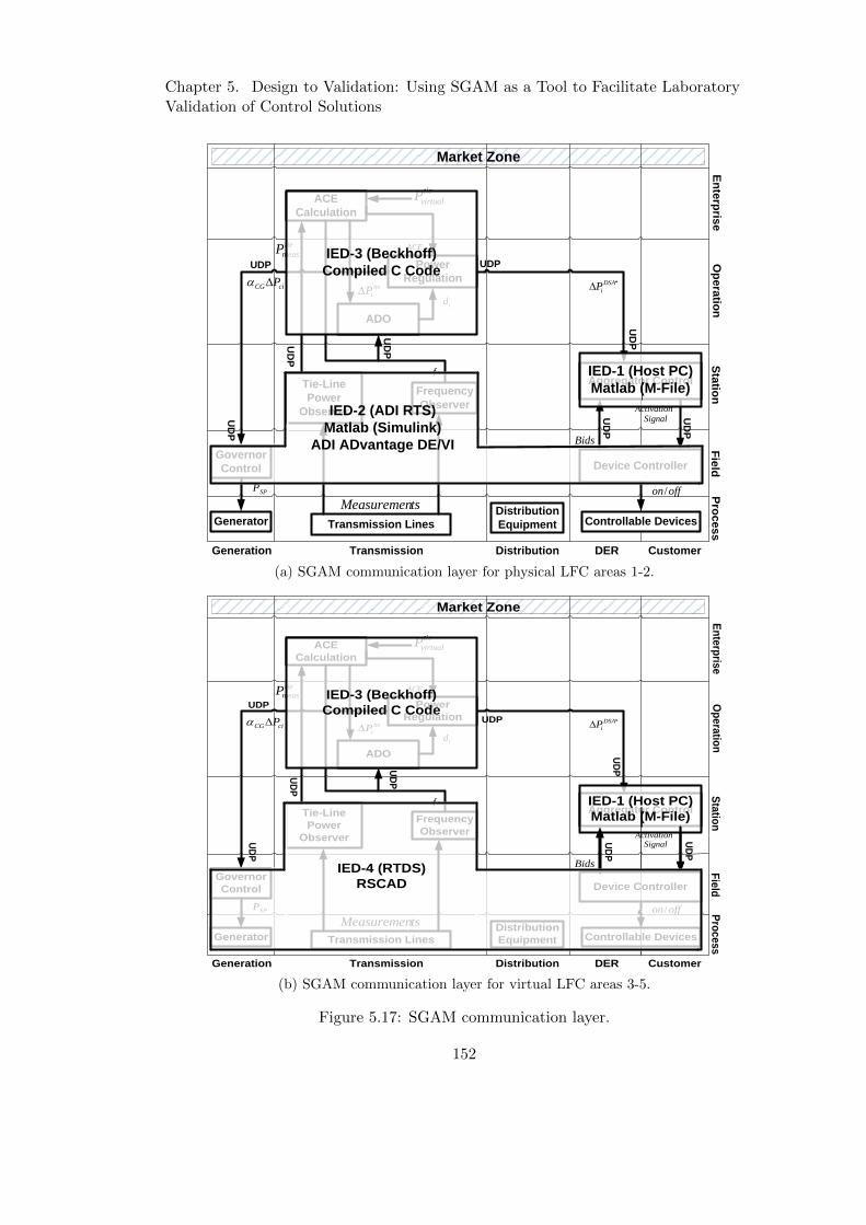
Chapter 5. Design to Validation: Using SGAM as a Tool to Facilitate LaboratoryValidation of Control Solutions
Aggregator Control
ACE
Calculation
Tie-Line
Power
Observer
ADO
Distribution DER Customer
Pro
ce
ss
Fie
ldS
tatio
nO
pe
ratio
nE
nte
rpris
e
Power
Regulation
Device Controller
Market Zone
Frequency
Observer
Governor
Control
TransmissionGeneration
GeneratorDistribution
Equipment Controllable DevicesTransmission Lines
id
tie
iP
iACE
f
*DSA
iP
tie
measP
tie
virtualP
Bids
ActivationSignal
SPP offon/
tsMeasuremen
IED-3 (Beckhoff)
Compiled C Code
IED-1 (Host PC)
Matlab (M-File)
IED-2 (ADI RTS)
Matlab (Simulink)
ADI ADvantage DE/VI
UD
P
UD
P
UDP
UD
P
UD
P
UD
P
UD
P
UDP
ciCG P
(a) SGAM communication layer for physical LFC areas 1-2.
Aggregator Control
ACE
Calculation
Tie-Line
Power
Observer
ADO
Distribution DER Customer
Pro
ce
ss
Fie
ldS
tatio
nO
pe
ratio
nE
nte
rpris
e
Power
Regulation
Device Controller
Market Zone
Frequency
Observer
Governor
Control
TransmissionGeneration
GeneratorDistribution
Equipment Controllable DevicesTransmission Lines
id
tie
iP
iACE
f
*DSA
iP
tie
measP
tie
virtualP
Bids
ActivationSignal
SPP offon/
tsMeasuremen
IED-3 (Beckhoff)
Compiled C Code
IED-1 (Host PC)
Matlab (M-File)
ciCG P
IED-4 (RTDS)
RSCAD
UD
P
UD
P
UD
P
UD
P
UDP
UDP
UD
P
UD
P
(b) SGAM communication layer for virtual LFC areas 3-5.
Figure 5.17: SGAM communication layer.
152
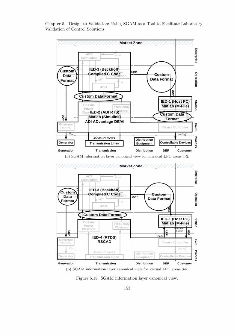
Chapter 5. Design to Validation: Using SGAM as a Tool to Facilitate LaboratoryValidation of Control Solutions
Aggregator Control
ACE
Calculation
Tie-Line
Power
Observer
ADO
Distribution DER Customer
Pro
ce
ss
Fie
ldS
tatio
nO
pe
ratio
nE
nte
rpris
e
Power
Regulation
Device Controller
Market Zone
Frequency
Observer
Governor
Control
TransmissionGeneration
GeneratorDistribution
Equipment Controllable DevicesTransmission Lines
id
tie
iP
iACE
f
*DSA
iPciCG P
tie
measP
tie
virtualP
Bids
ActivationSignal
SPP offon/
tsMeasuremen
IED-3 (Beckhoff)
Compiled C Code
IED-1 (Host PC)
Matlab (M-File)
IED-2 (ADI RTS)
Matlab (Simulink)
ADI ADvantage DE/VI
UD
P
UD
P
UDP
UD
P
UD
P
UD
P
UD
P
UDPCustom
Data
Format
Custom
Data Format
Custom Data Format
Custom Data
Format
(a) SGAM information layer canonical view for physical LFC areas 1-2.
Aggregator Control
ACE
Calculation
Tie-Line
Power
Observer
ADO
Distribution DER Customer
Pro
ce
ss
Fie
ldS
tatio
nO
pe
ratio
nE
nte
rpris
e
Power
Regulation
Device Controller
Market Zone
Frequency
Observer
Governor
Control
TransmissionGeneration
GeneratorDistribution
Equipment Controllable DevicesTransmission Lines
id
tie
iP
iACE
f
*DSA
iP
tie
measP
tie
virtualP
Bids
ActivationSignal
SPP offon/
tsMeasuremen
IED-3 (Beckhoff)
Compiled C Code
IED-1 (Host PC)
Matlab (M-File)
ciCG P
IED-4 (RTDS)
RSCAD
UD
P
UD
P
UD
P
UD
P
UDP
UDP
UD
P
UD
P
Custom
Data Format
Custom Data Format
Custom
Data
Format
(b) SGAM information layer canonical view for virtual LFC areas 3-5.
Figure 5.18: SGAM information layer canonical view.
153
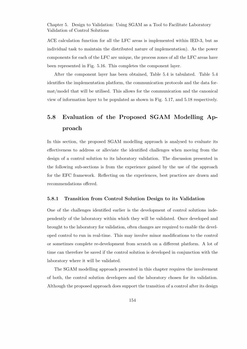
Chapter 5. Design to Validation: Using SGAM as a Tool to Facilitate LaboratoryValidation of Control Solutions
ACE calculation function for all the LFC areas is implemented within IED-3, but as
individual task to maintain the distributed nature of implementation). As the power
components for each of the LFC are unique, the process zones of all the LFC areas have
been represented in Fig. 5.16. This completes the component layer.
After the component layer has been obtained, Table 5.4 is tabulated. Table 5.4
identifies the implementation platform, the communication protocols and the data for-
mat/model that will be utilised. This allows for the communication and the canonical
view of information layer to be populated as shown in Fig. 5.17, and 5.18 respectively.
5.8 Evaluation of the Proposed SGAM Modelling Ap-
proach
In this section, the proposed SGAM modelling approach is analysed to evaluate its
effectiveness to address or alleviate the identified challenges when moving from the
design of a control solution to its laboratory validation. The discussion presented in
the following sub-sections is from the experience gained by the use of the approach
for the EFC framework. Reflecting on the experiences, best practices are drawn and
recommendations offered.
5.8.1 Transition from Control Solution Design to its Validation
One of the challenges identified earlier is the development of control solutions inde-
pendently of the laboratory within which they will be validated. Once developed and
brought to the laboratory for validation, often changes are required to enable the devel-
oped control to run in real-time. This may involve minor modifications to the control
or sometimes complete re-development from scratch on a different platform. A lot of
time can therefore be saved if the control solution is developed in conjunction with the
laboratory where it will be validated.
The SGAM modelling approach presented in this chapter requires the involvement
of both, the control solution developers and the laboratory chosen for its validation.
Although the proposed approach does support the transition of a control after its design
154
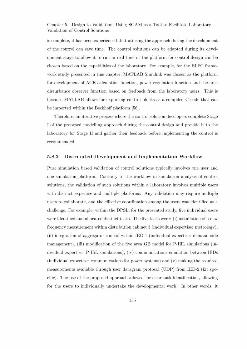
Chapter 5. Design to Validation: Using SGAM as a Tool to Facilitate LaboratoryValidation of Control Solutions
is complete, it has been experienced that utilising the approach during the development
of the control can save time. The control solutions can be adapted during its devel-
opment stage to allow it to run in real-time or the platform for control design can be
chosen based on the capabilities of the laboratory. For example, for the ELFC frame-
work study presented in this chapter, MATLAB Simulink was chosen as the platform
for development of ACE calculation function, power regulation function and the area
disturbance observer function based on feedback from the laboratory users. This is
because MATLAB allows for exporting control blocks as a compiled C code that can
be imported within the Beckhoff platform [56].
Therefore, an iterative process where the control solution developers complete Stage
I of the proposed modelling approach during the control design and provide it to the
laboratory for Stage II and gather their feedback before implementing the control is
recommended.
5.8.2 Distributed Development and Implementation Workflow
Pure simulation based validation of control solutions typically involves one user and
one simulation platform. Contrary to the workflow in simulation analysis of control
solutions, the validation of such solutions within a laboratory involves multiple users
with distinct expertise and multiple platforms. Any validation may require multiple
users to collaborate, and the effective coordination among the users was identified as a
challenge. For example, within the DPSL, for the presented study, five individual users
were identified and allocated distinct tasks. The five tasks were: (i) installation of a new
frequency measurement within distribution cabinet 3 (individual expertise: metrology),
(ii) integration of aggregator control within IED-1 (individual expertise: demand side
management), (iii) modification of the five area GB model for P-HiL simulations (in-
dividual expertise: P-HiL simulations), (iv) communications emulation between IEDs
(individual expertise: communications for power systems) and (v) making the required
measurements available through user datagram protocol (UDP) from IED-2 (kit spe-
cific). The use of the proposed approach allowed for clear task identification, allowing
for the users to individually undertake the developmental work. In other words, it
155
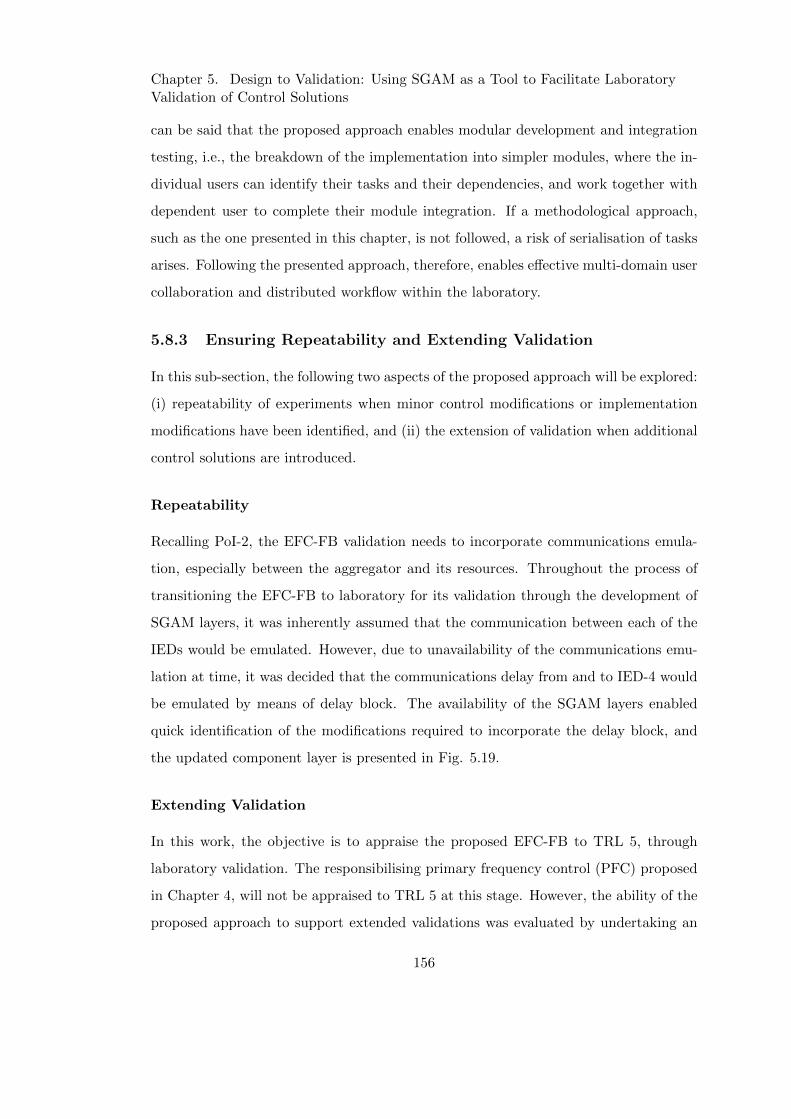
Chapter 5. Design to Validation: Using SGAM as a Tool to Facilitate LaboratoryValidation of Control Solutions
can be said that the proposed approach enables modular development and integration
testing, i.e., the breakdown of the implementation into simpler modules, where the in-
dividual users can identify their tasks and their dependencies, and work together with
dependent user to complete their module integration. If a methodological approach,
such as the one presented in this chapter, is not followed, a risk of serialisation of tasks
arises. Following the presented approach, therefore, enables effective multi-domain user
collaboration and distributed workflow within the laboratory.
5.8.3 Ensuring Repeatability and Extending Validation
In this sub-section, the following two aspects of the proposed approach will be explored:
(i) repeatability of experiments when minor control modifications or implementation
modifications have been identified, and (ii) the extension of validation when additional
control solutions are introduced.
Repeatability
Recalling PoI-2, the EFC-FB validation needs to incorporate communications emula-
tion, especially between the aggregator and its resources. Throughout the process of
transitioning the EFC-FB to laboratory for its validation through the development of
SGAM layers, it was inherently assumed that the communication between each of the
IEDs would be emulated. However, due to unavailability of the communications emu-
lation at time, it was decided that the communications delay from and to IED-4 would
be emulated by means of delay block. The availability of the SGAM layers enabled
quick identification of the modifications required to incorporate the delay block, and
the updated component layer is presented in Fig. 5.19.
Extending Validation
In this work, the objective is to appraise the proposed EFC-FB to TRL 5, through
laboratory validation. The responsibilising primary frequency control (PFC) proposed
in Chapter 4, will not be appraised to TRL 5 at this stage. However, the ability of the
proposed approach to support extended validations was evaluated by undertaking an
156
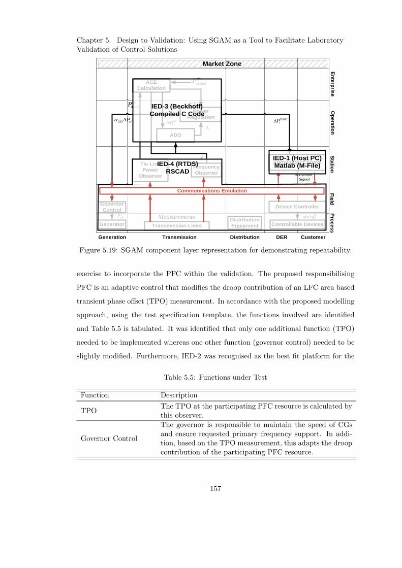
Chapter 5. Design to Validation: Using SGAM as a Tool to Facilitate LaboratoryValidation of Control Solutions
Aggregator Control
ACE
Calculation
Tie-Line
Power
Observer
ADO
Distribution DER Customer
Pro
ce
ss
Fie
ldS
tatio
nO
pe
ratio
nE
nte
rpris
e
Power
Regulation
Device Controller
Market Zone
Frequency
Observer
Governor
Control
TransmissionGeneration
GeneratorDistribution
Equipment Controllable DevicesTransmission Lines
id
tie
iP
iACE
f
*DSA
iP
tie
measP
tie
virtualP
Bids
ActivationSignal
SPP offon/tsMeasuremen
IED-3 (Beckhoff)
Compiled C Code
IED-1 (Host PC)
Matlab (M-File)IED-4 (RTDS)
RSCAD
ciCG P
Communications Emulation
Figure 5.19: SGAM component layer representation for demonstrating repeatability.
exercise to incorporate the PFC within the validation. The proposed responsibilising
PFC is an adaptive control that modifies the droop contribution of an LFC area based
transient phase offset (TPO) measurement. In accordance with the proposed modelling
approach, using the test specification template, the functions involved are identified
and Table 5.5 is tabulated. It was identified that only one additional function (TPO)
needed to be implemented whereas one other function (governor control) needed to be
slightly modified. Furthermore, IED-2 was recognised as the best fit platform for the
Table 5.5: Functions under Test
Function Description
TPOThe TPO at the participating PFC resource is calculated bythis observer.
Governor Control
The governor is responsible to maintain the speed of CGsand ensure requested primary frequency support. In addi-tion, based on the TPO measurement, this adapts the droopcontribution of the participating PFC resource.
157
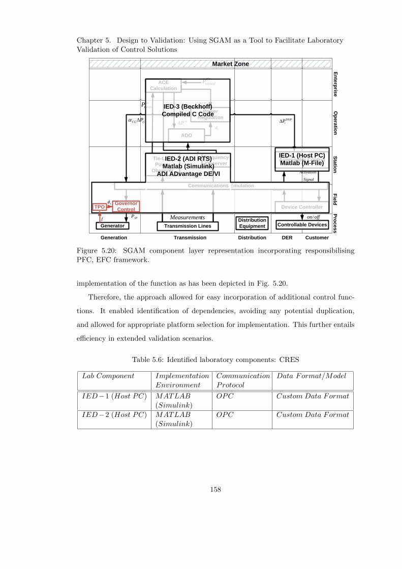
Chapter 5. Design to Validation: Using SGAM as a Tool to Facilitate LaboratoryValidation of Control Solutions
Aggregator Control
ACE
Calculation
Tie-Line
Power
Observer
ADO
Distribution DER Customer
Pro
ce
ss
Fie
ldS
tatio
nO
pe
ratio
nE
nte
rpris
e
Power
Regulation
Device Controller
Market Zone
Frequency
Observer
TransmissionGeneration
GeneratorDistribution
Equipment Controllable DevicesTransmission Lines
id
tie
iP
iACE
f
*DSA
iP
tie
measP
tie
virtualP
Bids
Activation
Signal
SPP offon/tsMeasuremen
IED-3 (Beckhoff)
Compiled C Code
IED-1 (Host PC)
Matlab (M-File)
Communications Emulation
IED-2 (ADI RTS)
Matlab (Simulink)
ADI ADvantage DE/VI
ciCG P
TPO
f
o Governor
Control
Figure 5.20: SGAM component layer representation incorporating responsibilisingPFC, EFC framework.
implementation of the function as has been depicted in Fig. 5.20.
Therefore, the approach allowed for easy incorporation of additional control func-
tions. It enabled identification of dependencies, avoiding any potential duplication,
and allowed for appropriate platform selection for implementation. This further entails
efficiency in extended validation scenarios.
Table 5.6: Identified laboratory components: CRES
Lab Component ImplementationEnvironment
CommunicationProtocol
Data Format/Model
IED−1 (Host PC) MATLAB(Simulink)
OPC Custom Data Format
IED−2 (Host PC) MATLAB(Simulink)
OPC Custom Data Format
158
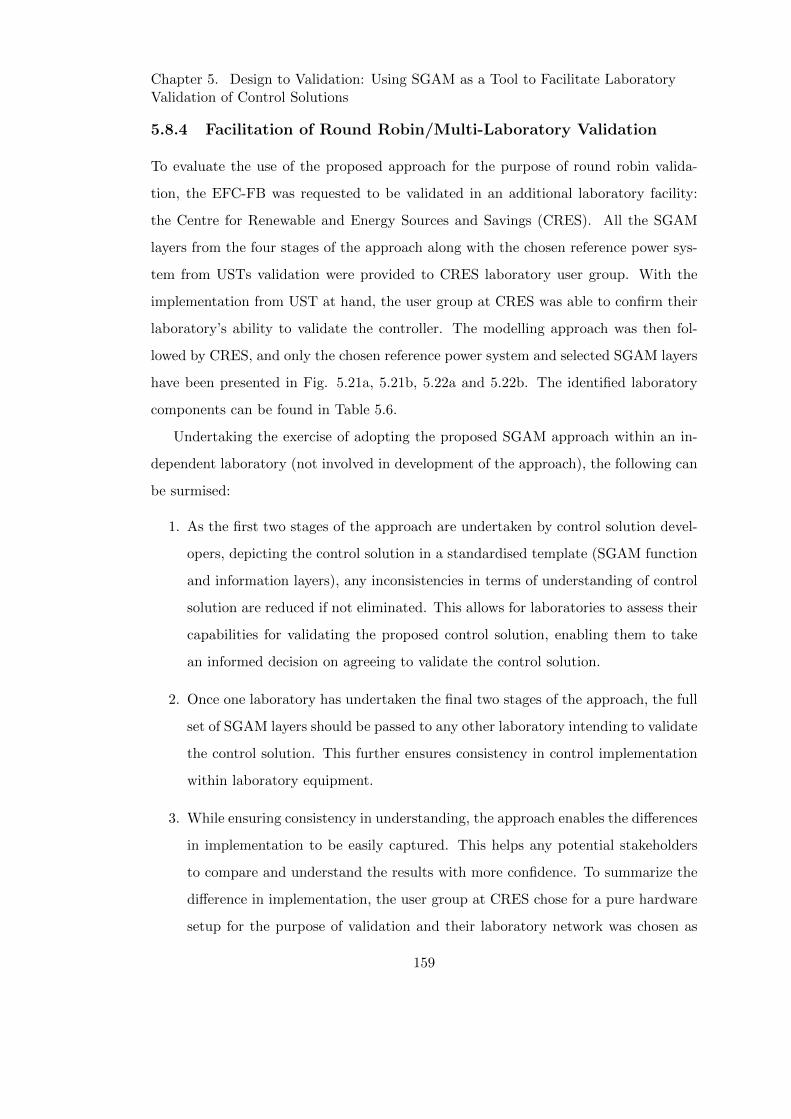
Chapter 5. Design to Validation: Using SGAM as a Tool to Facilitate LaboratoryValidation of Control Solutions
5.8.4 Facilitation of Round Robin/Multi-Laboratory Validation
To evaluate the use of the proposed approach for the purpose of round robin valida-
tion, the EFC-FB was requested to be validated in an additional laboratory facility:
the Centre for Renewable and Energy Sources and Savings (CRES). All the SGAM
layers from the four stages of the approach along with the chosen reference power sys-
tem from USTs validation were provided to CRES laboratory user group. With the
implementation from UST at hand, the user group at CRES was able to confirm their
laboratory’s ability to validate the controller. The modelling approach was then fol-
lowed by CRES, and only the chosen reference power system and selected SGAM layers
have been presented in Fig. 5.21a, 5.21b, 5.22a and 5.22b. The identified laboratory
components can be found in Table 5.6.
Undertaking the exercise of adopting the proposed SGAM approach within an in-
dependent laboratory (not involved in development of the approach), the following can
be surmised:
1. As the first two stages of the approach are undertaken by control solution devel-
opers, depicting the control solution in a standardised template (SGAM function
and information layers), any inconsistencies in terms of understanding of control
solution are reduced if not eliminated. This allows for laboratories to assess their
capabilities for validating the proposed control solution, enabling them to take
an informed decision on agreeing to validate the control solution.
2. Once one laboratory has undertaken the final two stages of the approach, the full
set of SGAM layers should be passed to any other laboratory intending to validate
the control solution. This further ensures consistency in control implementation
within laboratory equipment.
3. While ensuring consistency in understanding, the approach enables the differences
in implementation to be easily captured. This helps any potential stakeholders
to compare and understand the results with more confidence. To summarize the
difference in implementation, the user group at CRES chose for a pure hardware
setup for the purpose of validation and their laboratory network was chosen as
159
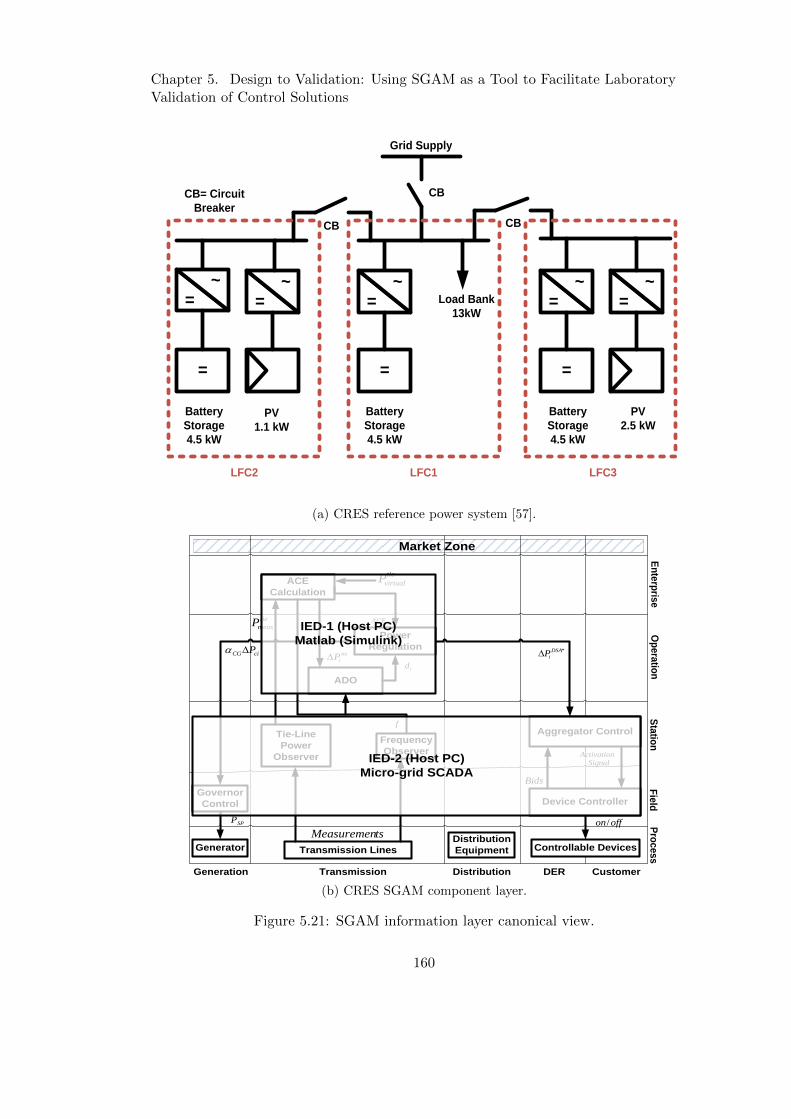
Chapter 5. Design to Validation: Using SGAM as a Tool to Facilitate LaboratoryValidation of Control Solutions
Load Bank
13kW=
~
=
Battery
Storage
4.5 kW
=
~
=
=
~
PV
1.1 kW
=
~
=
Battery
Storage
4.5 kW
=
~
PV
2.5 kW
Battery
Storage
4.5 kW
Grid Supply
CB CB
CBCB= Circuit
Breaker
LFC1LFC2 LFC3
(a) CRES reference power system [57].
Aggregator Control
ACE
Calculation
Tie-Line
Power
Observer
ADO
Distribution DER Customer
Pro
ce
ss
Fie
ldS
tatio
nO
pe
ratio
nE
nte
rpris
e
Power
Regulation
Device Controller
Market Zone
Frequency
Observer
Governor
Control
TransmissionGeneration
GeneratorDistribution
Equipment Controllable DevicesTransmission Lines
id
tie
iP
iACE
f
*DSA
iP
tie
measP
tie
virtualP
Bids
ActivationSignal
SPP offon/
tsMeasuremen
ciCG P
IED-1 (Host PC)
Matlab (Simulink)
IED-2 (Host PC)
Micro-grid SCADA
(b) CRES SGAM component layer.
Figure 5.21: SGAM information layer canonical view.
160
Chapter 5. Design to Validation: Using SGAM as a Tool to Facilitate LaboratoryValidation of Control Solutions
Market Zone
Enterprise ZoneOperation Zone
Field Zone
Pro
ce
ss
Generation Transmission Distribution DER Customer
Controllable
DevicesDistribution Equipment
Load Bank
13 kW
Distribution Cable
and Circuit Breaker
LF
C 1
Market Zone
Enterprise ZoneOperation Zone
Field Zone
Pro
ce
ss
Generation Transmission Distribution DER Customer
Controllable
DevicesDistribution Equipment
PV-1
1.1 kW
LF
C 2
Market Zone
Enterprise ZoneOperation Zone
Field Zone
Pro
ce
ss
Generation Transmission Distribution DER Customer
Controllable
DevicesDistribution Equipment
PV-2
2.5 kW
LF
C 3
Distribution Cable
and Circuit Breaker
Distribution Cable
and Circuit Breaker
Convertor
4.5 kW
Convertor
4.5 kW
Convertor
4.5 kW
(a) CRES SGAM component layer process zones for all LFCs.
OPC
OP
C
OP
C
Aggregator Control
ACE
Calculation
Tie-Line
Power
Observer
ADO
Distribution DER Customer
Pro
ce
ss
Fie
ldS
tatio
nO
pe
ratio
nE
nte
rpris
e
Power
Regulation
Device Controller
Market Zone
Frequency
Observer
Governor
Control
TransmissionGeneration
GeneratorDistribution
Equipment Controllable DevicesTransmission Lines
id
tie
iP
iACE
f
*DSA
iP
tie
measP
tie
virtualP
Bids
ActivationSignal
SPP offon/
tsMeasuremen
ciCG P
IED-1 (Host PC)
Matlab (Simulink)
IED-2 (Host PC)
Micro-grid SCADA
OP
C
OPCCustom
Data
Format
Custom
Data Format
Custom Data Format
(b) CRES SGAM information layer canonical view for all LFCs.
Figure 5.22: SGAM information layer canonical view.
161
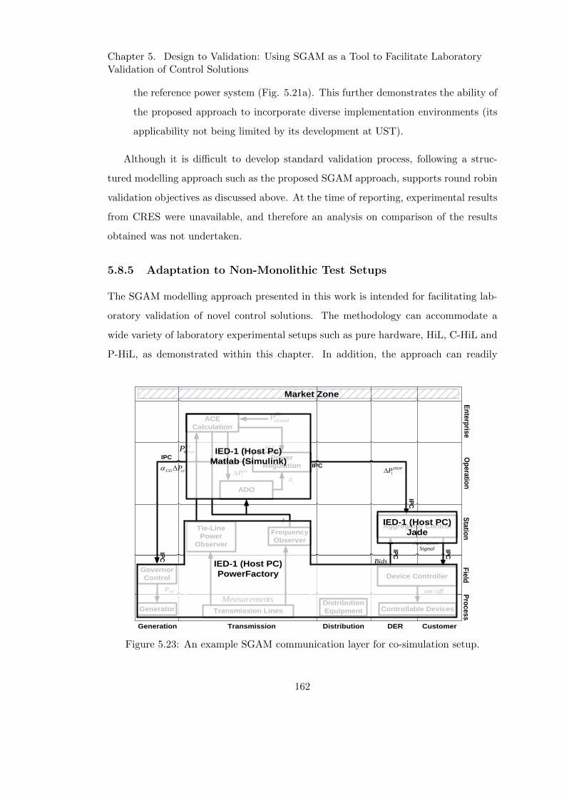
Chapter 5. Design to Validation: Using SGAM as a Tool to Facilitate LaboratoryValidation of Control Solutions
the reference power system (Fig. 5.21a). This further demonstrates the ability of
the proposed approach to incorporate diverse implementation environments (its
applicability not being limited by its development at UST).
Although it is difficult to develop standard validation process, following a struc-
tured modelling approach such as the proposed SGAM approach, supports round robin
validation objectives as discussed above. At the time of reporting, experimental results
from CRES were unavailable, and therefore an analysis on comparison of the results
obtained was not undertaken.
5.8.5 Adaptation to Non-Monolithic Test Setups
The SGAM modelling approach presented in this work is intended for facilitating lab-
oratory validation of novel control solutions. The methodology can accommodate a
wide variety of laboratory experimental setups such as pure hardware, HiL, C-HiL and
P-HiL, as demonstrated within this chapter. In addition, the approach can readily
Aggregator Control
ACE
Calculation
Tie-Line
Power
Observer
ADO
Distribution DER Customer
Pro
ce
ss
Fie
ldS
tatio
nO
pe
ratio
nE
nte
rpris
e
Power
Regulation
Device Controller
Market Zone
Frequency
Observer
Governor
Control
TransmissionGeneration
GeneratorDistribution
Equipment Controllable DevicesTransmission Lines
id
tie
iP
iACE
f
*DSA
iP
tie
measP
tie
virtualP
Bids
ActivationSignal
SPP offon/
tsMeasuremen
ciCG P
IED-1 (Host Pc)
Matlab (Simulink)
IED-1 (Host PC)
Jade
IED-1 (Host PC)
PowerFactory
IPC
IPC
IPCIPC
IPC
IPC
Figure 5.23: An example SGAM communication layer for co-simulation setup.
162
Chapter 5. Design to Validation: Using SGAM as a Tool to Facilitate LaboratoryValidation of Control Solutions
be adapted and utilised for the purpose facilitating validation by any non-monolithic
setups such as those utilised within the paradigm of co-simulation. Although several
multi-domain simulators such as MATLAB Simulink and OpenModelica are available
to validate smart grid control solutions in a monolithic way, co-simulation is utilised
when more accurate validation by means of utilising domain specific simulation tools
is desired. For example, for the study presented in this chapter, three distinct domains
can be identified: (i) power systems, (ii) controls and (iii) multi-agent system (MAS).
For monolithic validation MATLAB Simulink can readily be utilised, however, more
domain specific simulation tools exist for a thorough evaluation and can be utilised
within a co-simulation setup. In Fig. 5.23, an example mapping for co-simulation
setup is presented. As can be observed from the figure, three distinct simulation tools
for each domain have been utilised, namely, PowerFactory for power systems, MATLAB
Simulink for controls and Jade for MAS. As is common for co-simulation validation, all
the three simulation tools are within the same IED and Inter Process Communication
(IPC) is referred to as the common communication standard. When multiple IEDs are
utilised, this can be easily captured within the mappings as earlier presented.
5.9 Conclusions
In this chapter, the transition of a control from its design to its validation is discussed.
The key conclusions of the chapter are summarised below:
• The practical challenges that arise from the integration of control solutions within
laboratory environments, for their validation, are identified. These practical chal-
lenges have been given little or no importance in the past, however, with increasing
recognition of laboratory validations, to the best of authors knowledge, this is the
first attempt at reporting these challenges.
• The challenges identified were correlated to a lack of an integrated methodology.
To address this issue of lack of an integrated methodology, a structured approach
that utilizes SGAM as a tool to facilitate laboratory validations is proposed.
163
Chapter 5. Design to Validation: Using SGAM as a Tool to Facilitate LaboratoryValidation of Control Solutions
• As per the proposed SGAM modelling approach, any control solution to be vali-
dated is first represented using the SGAM followed by adding the representation
of the laboratory infrastructure which will validate the control solution. The
structured approach that leads to combined representation of control solutions
and laboratory infrastructure, in other words a validation environment, using the
SGAM facilitates the transition from the design of radical grid control solutions,
to their rigorous validation.
• The proposed SGAM modelling approach is applied to transition the EFC frame-
work to laboratory for its validation. This served two purposes: (i) it allowed
for developing the validation environment for the EFC-FB as is required for its
appraisal to TRL 5, and (ii) served as a basis for evaluating the proposed SGAM
modelling approach.
• An evaluation of the proposed SGAM modelling approach, apprised by the exer-
cise of its application to EFC framework, is presented. The key findings can be
summarised as:
– The proposed SGAM modelling approach encourages cooperation of con-
trol solution developers and laboratory user groups from the design stage,
entailing efficiency to the process.
– The proposed SGAM modelling approach is laboratory independent, i.e.,
it supports representation of any non-monolithic validation setups, evident
from its adoption in an independent smart grid laboratory (apart from DPSL
where the approach was developed) and its adoption for example represen-
tation of a co-simulation setup.
– The proposed SGAM modelling approach enhances: (i) repeatability after
modification to a control solution or its implementation, or when additional
control functions are incorporated, extending the scope of validation, and
(ii) reproducibility, enabling independent laboratories to develop tailored
validation environments for control solutions based on an example provided.
164

Chapter 5. Design to Validation: Using SGAM as a Tool to Facilitate LaboratoryValidation of Control Solutions
In essence, by enhancing repeatability and reproducibility of control solution
validation, the proposed approach supports round robin validations.
• The conventional SGAM modelling approach is limited to representation of con-
trol solutions implemented within a single entity (for example, one DSO, one
TSO, one LFC area, etc.). For the first time in this chapter, a concept to repre-
sent a control solution implemented within more than one entity is introduced.
The concept still requires two individual SGAM representations, one for each
entity, but enables capturing the information exchange between the two enti-
ties. This extends the ability of SGAM to represent distributed control solutions
implemented between the entities.
• Consequently, for the first time, two state-of-the-art smart grid laboratories have
been represented using the SGAM. The proposed SGAM modelling approach
presents an effective way to communicate research infrastructure features for in-
tegration and validation of control solutions.
165

Chapter 5. Design to Validation: Using SGAM as a Tool to Facilitate LaboratoryValidation of Control Solutions
REFERENCES
[1] E. Widl, P. Palensky, P. Siano, C. Rehtanz, “Guest editorial modeling, simulation,
and application of cyber-physical energy systems”, in IEEE Trans. Industrial
Informatics, Volume10, issue4, pp-2244-2246, 2014.
[2] T. I. Strasser, F. Andren, G. Lauss, R. Brundlinger, H. Brunner, C. Moyo, C.
Seitl, S. Rohjans, S. Lehnhoff, P. Palensky, P. Kotsampopoulos N. Hatziargyriou,
G. Arnold, W. Heckmann, E. Jong, M. Verga, G. Franchioni, L. Martini, A.
Kosek, O. Gehrke, H. Bindner, F. Coffele, G. Burt, M. Calin, E. Rodriguez-Seco
“Towards holistic power distribution system validation and testing—an overview
and discussion of different possibilities”, in e & I Elektrotechnik und Information-
stechnik, pp. 71-77, 2017.
[3] “Smart Grids: from innovation to deployment”, European Commission, Com-
munication from the Commission to the European Parliament, the Council, the
European Economic and Social Committee and the Committee of the Regions,
2011.
[4] “Roadmap 2010-18 and detailed implementation plan 2010-12”, European Elec-
tricity Grid Initiative (EEGI), 2010.
[5] M. Maniatopoulos, D. Lagos, P. Kotsampopoulos, and N. Hatziargyriou, “Com-
bined control and power hardware in-the-loop simulation for testing smart grid
control algorithms”, inIET Generation, Transmission and Distribution, vol. 11,
no. 12, pp. 3009-3018, 2017.
[6] A. Gil de Muro, J. E. Rodriguez-Seco, E. Zabala, C. Mayr, R. Brundlinger,
G. Romanovsky, O. Gehrke, and F. Isleifsson, “Inverter interconnection tests
performed in the LABEIN-Tecnalia microgrid involved in the DERlab round-
robin testing activity”, in proceedings of the International Conference Electrical
Power Quality and Utilisation, Lodz, pp. 1-5, 2009.
[7] R. Brundlinger, T. I. Strasser, G. Lauss, A. Hoke, S. Chakraborty, G. Martin, B.
166
Chapter 5. Design to Validation: Using SGAM as a Tool to Facilitate LaboratoryValidation of Control Solutions
Kroposki, J. Johnson, and E. Jong, “Lab tests: verifying that Smart Grid power
converters are truly smart”, in IEEE Power Energy Magazine, pp. 30-42, 2015.
[8] J. Belanger, P. Venne, J.-N, Paquin, “The what, where, and why of real-time
simulation”, Planet RT. 37-49, 2010.
[9] M. Muresan, D. Pitica, “Software in the loop environment reliability for testing
embedded code”, in proceedings of IEEE 18th International Symposium for De-
sign and Technology in Electronic Packaging, Alba Iulia, Romania, pp. 325-328,
October 2012.
[10] S. Werner, L. Masing, F. Lesniak, and J. Becker, “Software-in-the-loop simulation
of embedded control applications based on virtual platforms”, in proceedings of
25th International Conference on Field Programmable Logic Applications, Lon-
don, England, pp. 1-8, September 2015.
[11] “PSSE User Manual v30.2, Siemens Power Transmission & Distribution”, Siemens
Power Technologies International Inc., 2005.
[12] M. Perron, E. Ghahremani, A. Heniche, I. Kamwa, C. Lafond, M. Racine, H.
Akremi, P. Cadieux, S. Lebeau, and S. Landry, “Wide-area voltage control system
of flexible AC transmission system devices to prevent voltage collapse”, in IET
Generation, Transmission and Distribution, vol. 11, no. 18, pp. 4556-4564, 2017.
[13] J. Coser, A. S. Costa and J. G. Rolim,“Metering Scheme Optimization With
Emphasis on Ensuring Bad-Data Processing Capability”, in IEEE Trans. on
Power Systems, vol. 21, no. 4, pp. 1903-1911, Nov. 2006.
[14] J. Xu, C. Zhao, W. Liu and C. Guo, “Accelerated Model of Modular Multilevel
Converters in PSCAD/EMTDC”, in IEEE Trans. on Power Delivery, vol. 28,
no. 1, pp. 129-136, Jan. 2013.
[15] X. Wu, V. Simha, Y. Xue and R. Wellman, “Substation Grounding Studies with
More Accurate Fault Simulation Strategy and SI / MI Method”, in IEEE Trans.
on Power Delivery, vol. PP no. 99, pp. 1-1, 2018.
167
Chapter 5. Design to Validation: Using SGAM as a Tool to Facilitate LaboratoryValidation of Control Solutions
[16] J. Tant and J. Driesen, ”On the Numerical Accuracy of Electromagnetic Transient
Simulation with Power Electronics,” in IEEE Trans. on Power Delivery, vol. PP
no. 99, pp. 1-1, 2018.
[17] K. Johnstone, S. M. Blair, M. H. Syed, A. Emhemed, G. M. Burt and T. I.
Strasser, ”Co-simulation approach using PowerFactory and MATLAB/Simulink
to enable validation of distributed control concepts within future power systems,”
in CIRED - Open Access Proceedings Journal, vol. 2017, no. 1, pp. 2192-2196,
10 2017.
[18] T. I. Strasser, M. Stifter, F. Andren, and P. Palensky, “Co-simulation training
platform for smart grids”, in IEEE Trans. on Power Systems, 1989-1997, 2014.
[19] C. Steinbrink, S. Lehnhoff, S. Rohjans, T. I. Strasser, E. Widl, C. Moyo, G.
Lauss, F. Lehfuss, M. Faschang, P. Palensky, A. A. van der Meer, K. Heussen, O.
Gehrke, E. Guillo-Sansano, M. H. Syed, A. Emhemed, R. Brandl, V. H. Nguyen,
A. Khavari, Q. T. Tran, P. Kotsampopoulos, N. Hatziargyriou, N. Akroud, E.
Rikos, and M. Z. Degefa “Simulation-based validation of smart grids - status quo
and future research trends”, in Proc. Int. Conf. on Ind. Appl. of Holonic and
Multi-Agent Syst., Lyon, pp. 171-185, 2017.
[20] J. Jeon, J. Kim, H. Kim, S. Kim, C. Cho, J. Kim, J. Ahn, and K. Nam “De-
velopment of hardware in-the-loop simulation system for testing operation and
control functions of microgrid”, in IEEE Trans. on Power Electronics, 25, (12),
pp. 2919-2929, 2010.
[21] M. O. Faruque, and V. Dinavahi, “Hardware-in-the-loop simulation of power
electronic system using adaptive discretization”,in IEEE Trans. on Industrial
Electronics, pp. 1146-1158, 2010.
[22] J. Wang, Y. Song, W. Li, J. Guo, and A. Monti, “Development of a univer-
sal platform for hardware in-the-loop testing of microgrids”,in IEEE Trans. on
Industrial Informatics, pp. 2154-2165, 2014.
168
Chapter 5. Design to Validation: Using SGAM as a Tool to Facilitate LaboratoryValidation of Control Solutions
[23] P. Kotsampopoulos, F. Lehfuss, G. Lauss, B. Bletterie, and N. D. Hatziargyriou,
“The limitations of digital simulation and the advantages of PHIL testing in
studying distributed generation provision of ancillary services”, in IEEE Trans.
on Industrial Electronics, 62, (9), pp. 5502-5515, 2015.
[24] M. Steurer, C. S. Edrington, M. Sloderbeck, W. Ren, and J. Langston, “A
megawatt-scale power hardware-in-the-loop simulation setup for motor drives”,
inIEEE Trans. on Industrial Electronics, 57, (4), pp. 1254-1260, 2010.
[25] G. F. Lauss, M. O. Faruque, K. Schoder, C. Dufour, A. Viehweider, and J.
Langston, “Characteristics and design of power hardware-in-the-loop simulations
for electrical power systems”, in IEEE Trans. on Industrial Electronics, 63, (1),
pp. 406-417, 2015.
[26] M. Heder, “From NASA to EU: the evolution of the TRL scale in Public Sector
Innovation”, in The Innovation Journal, pp. 1-23, 2017.
[27] “Test protocols for advances inverter interoperability functions”, Sandia National
Laboratories, Sandia Corporation, pp 1-22, 2013.
[28] IEC/TR 61850 (2003-04), Communication networks and systems in substations.
[29] CIM Users Group’s Home Page, http://cimug.ucaiug.org/default.aspx
[30] “The Project”, https://erigrid.eu/the-project/
[31] B. Marick, “New Models for Test Development”, http://www.exampler.com/
testing-com/writings/new-models.pdf
[32] C. Bucanac, “The V-Model”, Quality Management, University of Karl-
skrona/Ronneby.
[33] T. Weilkiens, J. G. Lamm, S. Roth, and M. Walker, “Model based system archi-
tecture”, John Wiley and Sons.
169
Chapter 5. Design to Validation: Using SGAM as a Tool to Facilitate LaboratoryValidation of Control Solutions
[34] “What is V-model- advantages, disadvantages and
when to use it?”, http://istqbexamcertification.com/
what-is-v-model-advantages-disadvantages-and-when-to-use-it/
[35] R. S. Pressman, “Software Engineering: A Practitioner’s Approach”, The
McGraw-Hill Companies.
[36] M. Hoffman, and B. Beaumont, “Application Development: Managing the
Project Life Cycle”, Mc Press.
[37] “Standardization Mandate to European Standardisation Organisations (ESOs)
to support European Smart Grid deployment”, European Commission. [On-
line]. Available: https://ec.europa.eu/energy/sites/ener/files/documents/2011
03 01 mandate m490 en.pdf
[38] “NIST Framework and Roadmap for Smart Grid Interoperability, Interoperability
Standards Release 1.0”, Office of the National Coordinator for Smart Grid Inter-
operability, National Institute of Standards and Technology, U.S. Department of
Commerce, 2009.
[39] “GridWise Interoperability Context-Setting Framework”, 2008, GridWise Archi-
tecture Council, www.gridwiseac.org.
[40] “IntelliGrid Methodology for Developing Requirements for Energy Systems”,
IEC/PAS 62559. [Online]. Available: https://webstore.iec.ch/preview/info
iecpas62559%7Bed1.0%7Den.pdf
[41] “TOGAF 9 and ArchiMate 1.0 White paper”, The Open Group 2010, [Online].
Available: http://pubs.opengroup.org/architecture/togaf9-doc/arch/ and http:
//pubs.opengroup.org/architecture/archimate2-doc/
[42] “Smart Grid Coordination Group (SGCG) First Set of Standards”, CEN, CEN-
ELEC, and ETSI, Nov. 2012.
[43] R. Santodomingo, M. Uslar, A. Goring, M. Gottschalk, L. Nordstrom, A. Saleem,
and M. Chenine, “SGAM-based methodology to analyse Smart Grid solutions in
170
Chapter 5. Design to Validation: Using SGAM as a Tool to Facilitate LaboratoryValidation of Control Solutions
DISCERN European research project”, in proceedings of 2014 IEEE International
Energy Conference (ENERGYCON), Cavtat, pp. 751-758, 2014.
[44] “Annex I: Description of the Work”, Distributed Intelligence for Cost-Effective
and Reliable Distribution Network Operation (DISCERN) EU project, September
2012, http://www.discern.eu/
[45] “Deliverable D4.2: New system functionality”, Distributed Intelligence for Cost-
Effective and Reliable Distribution Network Operation (DISCERN), Jan. 2014.
[46] “Smart Grid Coordination Group (SGCG) Reference Architecture Smart Grid”,
CEN, CENELEC, and ETSI, Nov. 2012.
[47] “Smart Grid Coordination Group (SGCG) Methodology and New Applications”,
CEN, CENELEC, and ETSI, Dec. 2014.
[48] “Deliverable D1.3: Architecture templates and guidelines”, Distributed Intel-
ligence for Cost-Effective and Reliable Distribution Network Operation (DIS-
CERN), Nov. 2013.
[49] “Draft IEC 62559: Use Case Methodology – Part 2: Definition of the templates
for use cases, actor list and requirements list”, IEC TC8 Standard, Jun. 2013.
[50] Blank, S. Lehnhoff, K. Heussen, D. E. M. Bondy, C. Moyo, and T. Strasser,
“Towards a foundation for holistic power system validation and testing”, in pro-
ceedings of 2016 IEEE 21st International Conference on Emerging Technologies
and Factory Automation (ETFA), 2016.
[51] “Proposal for the bidding and activation process and balancing en-
ergy products for the bid ladder platform”, Elia. [online] Available:
http://www.elia.be/en/users-group/ad-hoc-taskforce-balancing/Bid-ladder-
platform.
[52] M. H. Syed, G.M. Burt, R. D’Hulst, and J. Verbeeck,“Experimental Validation
of Flexibility Provision by Highly Distributed Demand Portfolio”, in proceedings
of the 2016 CIRED Workshop, pp. 1-4, Helsinki, Finland, 2016.
171
Chapter 5. Design to Validation: Using SGAM as a Tool to Facilitate LaboratoryValidation of Control Solutions
[53] P. Dambrauskas, M. H. Syed, S. M. Blair, J. M. Irvine, I. F. Abdulhadi, G. M.
Burt, and D. E. M. Bondy ”Impact of realistic communications for fast-acting
demand side management,” in CIRED - Open Access Proceedings Journal, vol.
2017, no. 1, pp. 1813-1817, 10 2017.
[54] T. Magisos, “Real-time Simulation and Model-Based-Systems Engineering us-
ing Commercial-Off-The-Shelf (COTS) Computer Equipment”, Applied Dynam-
ics International (ADI). [Online]. Available: https://www.adi.com/wp-content/
uploads/2016/06/Real-time COTS Paper v1.7.pdf
[55] S. M. Blair, “Beckhoff and TwinCAT 3 System Development Guide” Report.
[Online]. Available https://strathprints.strath.ac.uk/55254/
[56] “Simulink Coder - Generate C and C++ code from Simulink
and Stateflow models”, MathWorks, 2012. [Online]. Available:
http://www.mathworks.co.uk/products/simulinkcoder/.
[57] A. Neris, S. Tselepis, and C. Protogeropoulos, “Description of a Simulated Micro-
grid Test Field Facility and Results from System Testing under Different Load
Control Strategies”, in proceedings of CIGRE Symposium, Power Systems with
Dispersed Generation, Athens, Greece, 13-16 April 2005.
172
Chapter 6
Appraisal of Fast Balancing
Enhanced Frequency Control to
TRL 5
6.1 Introduction
The validation of the fast balancing enhanced frequency control (EFC-FB) in real-time
has demonstrated the feasibility and soundness of the approach effectively appraising it
to technology readiness level (TRL) 3. With the three purpose of investigations (PoI)
set in Chapter 5, in this chapter, the EFC-FB is appraised to TRL 5. In accordance
with the PoI’s, first the results of controller hardware-in-the-loop (C-HiL) implemen-
tation are presented. This involves the prototypical implementation of the EFC-FB
within a controller hardware. This is followed by results from a C-HiL implementation
incorporating realistic communications delays. With the C-HiL validation, EFC-FB is
appraised to TRL 4. The incorporation of the reference power system, the five area
Great Britain (GB) power system, in a power hardware-in-the-loop (P-HiL) setup is
presented. This complex setup presented a challenge in terms of initialisation and
synchronisation, for which a range of alternatives are investigated and recommended
approach identified. This is followed by appraising the performance of EFC-FB under
173
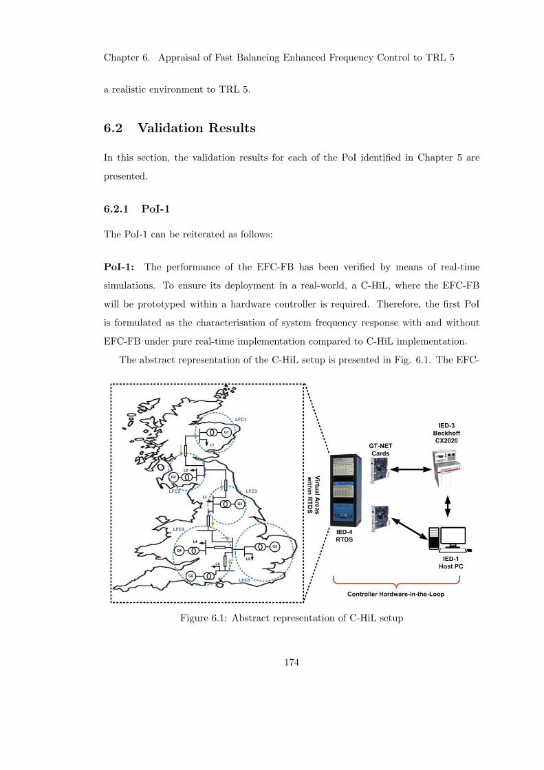
Chapter 6. Appraisal of Fast Balancing Enhanced Frequency Control to TRL 5
a realistic environment to TRL 5.
6.2 Validation Results
In this section, the validation results for each of the PoI identified in Chapter 5 are
presented.
6.2.1 PoI-1
The PoI-1 can be reiterated as follows:
PoI-1: The performance of the EFC-FB has been verified by means of real-time
simulations. To ensure its deployment in a real-world, a C-HiL, where the EFC-FB
will be prototyped within a hardware controller is required. Therefore, the first PoI
is formulated as the characterisation of system frequency response with and without
EFC-FB under pure real-time implementation compared to C-HiL implementation.
The abstract representation of the C-HiL setup is presented in Fig. 6.1. The EFC-
Figure 6.1: Abstract representation of C-HiL setup
174
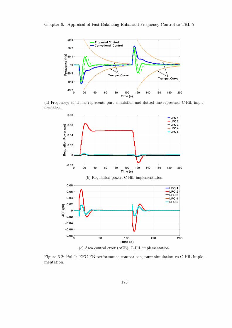
Chapter 6. Appraisal of Fast Balancing Enhanced Frequency Control to TRL 5
0 20 40 60 80 100 120 140 160 180 200
Time (s)
49.7
49.8
49.9
50
50.1
50.2
50.3
Fre
qu
en
cy (
Hz)
Trumpet CurveTrumpet Curve
Proposed ControlConvetional Control
(a) Frequency; solid line represents pure simulation and dotted line represents C-HiL imple-mentation.
0 20 40 60 80 100 120 140 160 180 200
Time (s)
-0.02
0
0.02
0.04
0.06
0.08
Reg
ula
tio
n P
ow
er
(pu
)
LFC 1
LFC 2
LFC 3
LFC 4
LFC 5
(b) Regulation power, C-HiL implementation.
0 50 100 150 200
Time (s)
-0.08
-0.06
-0.04
-0.02
0
0.02
0.04
0.06
0.08
AC
E (
pu
)
LFC 1
LFC 2
LFC 3
LFC 4
LFC 5
(c) Area control error (ACE), C-HiL implementation.
Figure 6.2: PoI-1: EFC-FB performance comparison, pure simulation vs C-HiL imple-mentation.
175
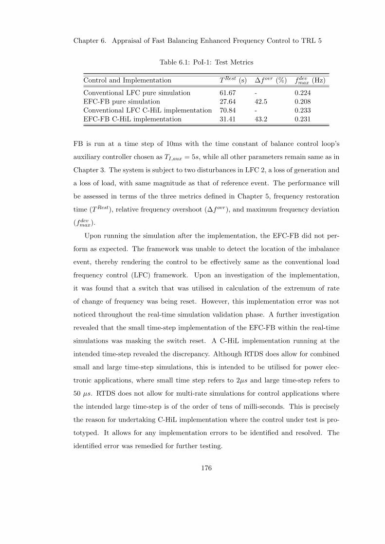
Chapter 6. Appraisal of Fast Balancing Enhanced Frequency Control to TRL 5
Table 6.1: PoI-1: Test Metrics
Control and Implementation TRest (s) ∆fovr (%) fdevmax (Hz)
Conventional LFC pure simulation 61.67 - 0.224EFC-FB pure simulation 27.64 42.5 0.208Conventional LFC C-HiL implementation 70.84 - 0.233EFC-FB C-HiL implementation 31.41 43.2 0.231
FB is run at a time step of 10ms with the time constant of balance control loop’s
auxiliary controller chosen as TI,aux = 5s, while all other parameters remain same as in
Chapter 3. The system is subject to two disturbances in LFC 2, a loss of generation and
a loss of load, with same magnitude as that of reference event. The performance will
be assessed in terms of the three metrics defined in Chapter 5, frequency restoration
time (TRest), relative frequency overshoot (∆fovr), and maximum frequency deviation
(fdevmax).
Upon running the simulation after the implementation, the EFC-FB did not per-
form as expected. The framework was unable to detect the location of the imbalance
event, thereby rendering the control to be effectively same as the conventional load
frequency control (LFC) framework. Upon an investigation of the implementation,
it was found that a switch that was utilised in calculation of the extremum of rate
of change of frequency was being reset. However, this implementation error was not
noticed throughout the real-time simulation validation phase. A further investigation
revealed that the small time-step implementation of the EFC-FB within the real-time
simulations was masking the switch reset. A C-HiL implementation running at the
intended time-step revealed the discrepancy. Although RTDS does allow for combined
small and large time-step simulations, this is intended to be utilised for power elec-
tronic applications, where small time step refers to 2µs and large time-step refers to
50 µs. RTDS does not allow for multi-rate simulations for control applications where
the intended large time-step is of the order of tens of milli-seconds. This is precisely
the reason for undertaking C-HiL implementation where the control under test is pro-
totyped. It allows for any implementation errors to be identified and resolved. The
identified error was remedied for further testing.
176
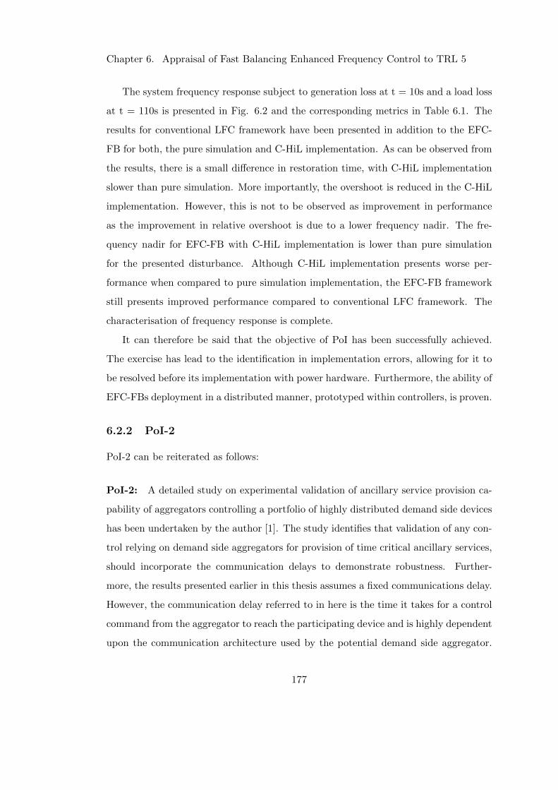
Chapter 6. Appraisal of Fast Balancing Enhanced Frequency Control to TRL 5
The system frequency response subject to generation loss at t = 10s and a load loss
at t = 110s is presented in Fig. 6.2 and the corresponding metrics in Table 6.1. The
results for conventional LFC framework have been presented in addition to the EFC-
FB for both, the pure simulation and C-HiL implementation. As can be observed from
the results, there is a small difference in restoration time, with C-HiL implementation
slower than pure simulation. More importantly, the overshoot is reduced in the C-HiL
implementation. However, this is not to be observed as improvement in performance
as the improvement in relative overshoot is due to a lower frequency nadir. The fre-
quency nadir for EFC-FB with C-HiL implementation is lower than pure simulation
for the presented disturbance. Although C-HiL implementation presents worse per-
formance when compared to pure simulation implementation, the EFC-FB framework
still presents improved performance compared to conventional LFC framework. The
characterisation of frequency response is complete.
It can therefore be said that the objective of PoI has been successfully achieved.
The exercise has lead to the identification in implementation errors, allowing for it to
be resolved before its implementation with power hardware. Furthermore, the ability of
EFC-FBs deployment in a distributed manner, prototyped within controllers, is proven.
6.2.2 PoI-2
PoI-2 can be reiterated as follows:
PoI-2: A detailed study on experimental validation of ancillary service provision ca-
pability of aggregators controlling a portfolio of highly distributed demand side devices
has been undertaken by the author [1]. The study identifies that validation of any con-
trol relying on demand side aggregators for provision of time critical ancillary services,
should incorporate the communication delays to demonstrate robustness. Further-
more, the results presented earlier in this thesis assumes a fixed communications delay.
However, the communication delay referred to in here is the time it takes for a control
command from the aggregator to reach the participating device and is highly dependent
upon the communication architecture used by the potential demand side aggregator.
177
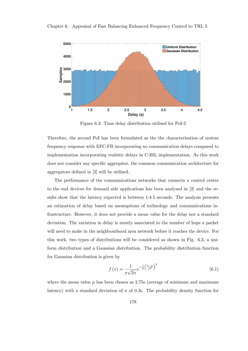
Chapter 6. Appraisal of Fast Balancing Enhanced Frequency Control to TRL 5
1 1.5 2 2.5 3 3.5 4 4.5
Delay (s)
0
1000
2000
3000
4000
5000
Sam
ple
s
Uniform Distribution
Gaussian Distribution
Figure 6.3: Time delay distribution utilised for PoI-2
Therefore, the second PoI has been formulated as the the characterisation of system
frequency response with EFC-FB incorporating no communication delays compared to
implementation incorporating realistic delays in C-HiL implementation. As this work
does not consider any specific aggregator, the common communication architecture for
aggregators defined in [2] will be utilised.
The performance of the communications networks that connects a control centre
to the end devices for demand side applications has been analysed in [2] and the re-
sults show that the latency expected is between 1-4.5 seconds. The analysis presents
an estimation of delay based on assumptions of technology and communications in-
frastructure. However, it does not provide a mean value for the delay nor a standard
deviation. The variation in delay is mostly associated to the number of hops a packet
will need to make in the neighbourhood area network before it reaches the device. For
this work, two types of distributions will be considered as shown in Fig. 6.3, a uni-
form distribution and a Gaussian distribution. The probability distribution function
for Gaussian distribution is given by
(6.1)f (x) =1
σ√
2πe− 1
2
(x−µσ2
)2
where the mean value µ has been chosen as 2.75s (average of minimum and maximum
latency) with a standard deviation of σ of 0.3s. The probability density function for
178
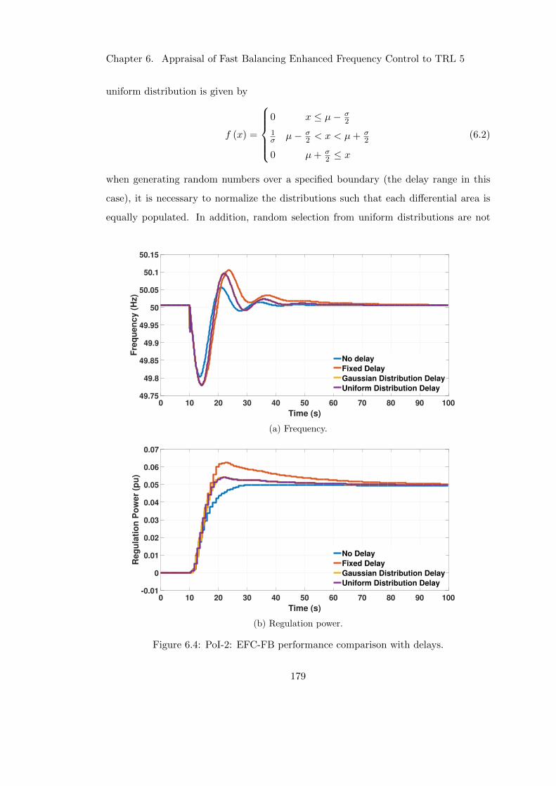
Chapter 6. Appraisal of Fast Balancing Enhanced Frequency Control to TRL 5
uniform distribution is given by
(6.2)f (x) =
0 x ≤ µ− σ
2
1σ µ− σ
2 < x < µ+ σ2
0 µ+ σ2 ≤ x
when generating random numbers over a specified boundary (the delay range in this
case), it is necessary to normalize the distributions such that each differential area is
equally populated. In addition, random selection from uniform distributions are not
0 10 20 30 40 50 60 70 80 90 100
Time (s)
49.75
49.8
49.85
49.9
49.95
50
50.05
50.1
50.15
Fre
qu
en
cy (
Hz)
No delay
Fixed Delay
Gaussian Distribution Delay
Uniform Distribution Delay
(a) Frequency.
0 10 20 30 40 50 60 70 80 90 100
Time (s)
-0.01
0
0.01
0.02
0.03
0.04
0.05
0.06
0.07
Reg
ula
tio
n P
ow
er
(pu
)
No Delay
Fixed Delay
Gaussian Distribution Delay
Uniform Distribution Delay
(b) Regulation power.
Figure 6.4: PoI-2: EFC-FB performance comparison with delays.
179
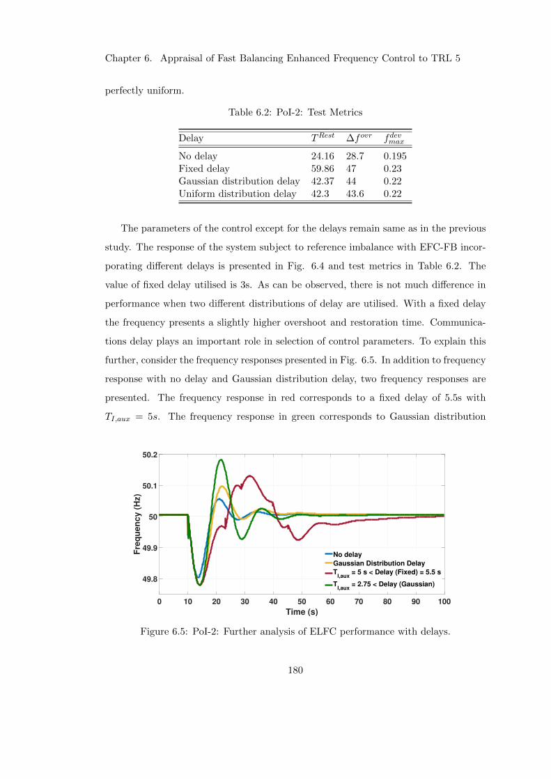
Chapter 6. Appraisal of Fast Balancing Enhanced Frequency Control to TRL 5
perfectly uniform.
Table 6.2: PoI-2: Test Metrics
Delay TRest ∆fovr fdevmax
No delay 24.16 28.7 0.195Fixed delay 59.86 47 0.23Gaussian distribution delay 42.37 44 0.22Uniform distribution delay 42.3 43.6 0.22
The parameters of the control except for the delays remain same as in the previous
study. The response of the system subject to reference imbalance with EFC-FB incor-
porating different delays is presented in Fig. 6.4 and test metrics in Table 6.2. The
value of fixed delay utilised is 3s. As can be observed, there is not much difference in
performance when two different distributions of delay are utilised. With a fixed delay
the frequency presents a slightly higher overshoot and restoration time. Communica-
tions delay plays an important role in selection of control parameters. To explain this
further, consider the frequency responses presented in Fig. 6.5. In addition to frequency
response with no delay and Gaussian distribution delay, two frequency responses are
presented. The frequency response in red corresponds to a fixed delay of 5.5s with
TI,aux = 5s. The frequency response in green corresponds to Gaussian distribution
0 10 20 30 40 50 60 70 80 90 100
Time (s)
49.8
49.9
50
50.1
50.2
Fre
qu
en
cy (
Hz)
No delay
Gaussian Distribution Delay
TI,aux
= 5 s < Delay (Fixed) = 5.5 s
TI,aux
= 2.75 < Delay (Gaussian)
Figure 6.5: PoI-2: Further analysis of ELFC performance with delays.
180
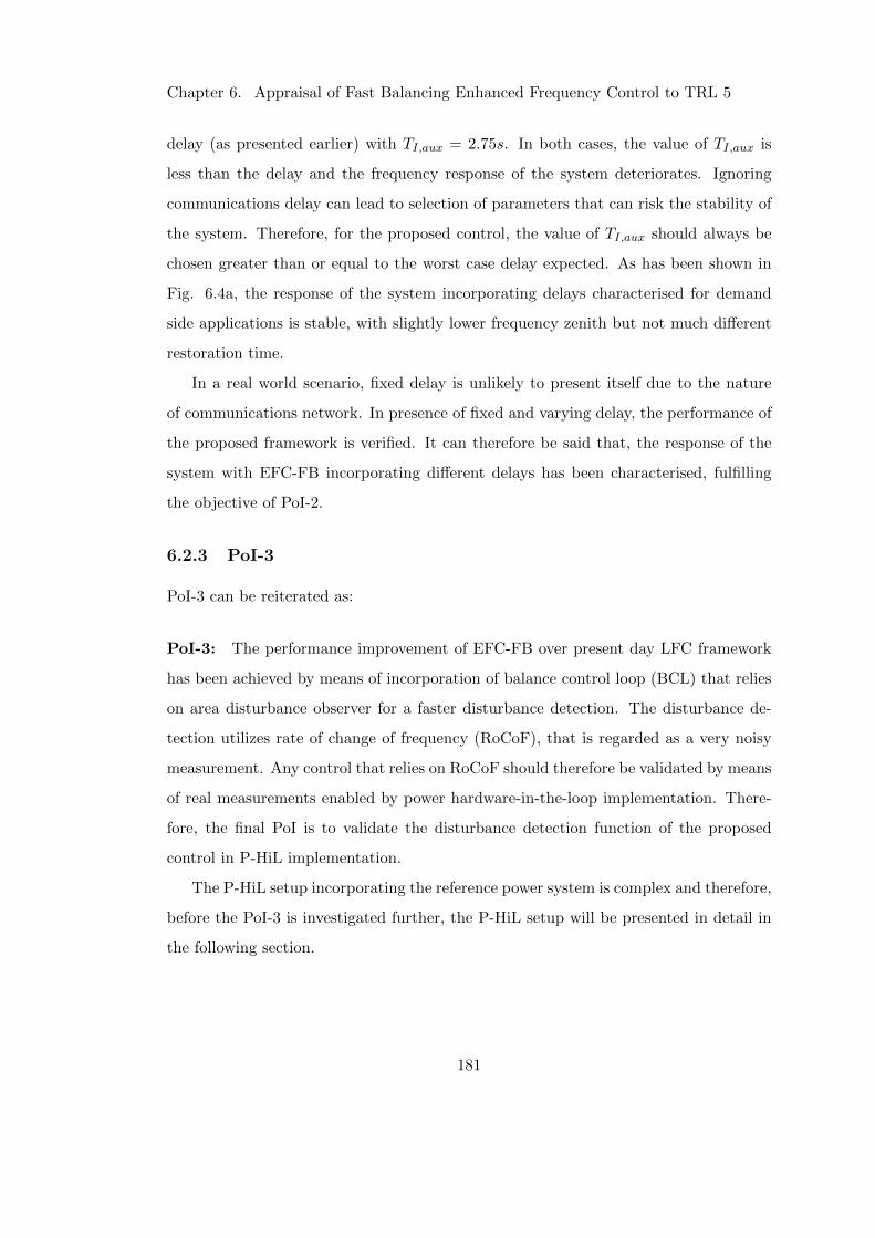
Chapter 6. Appraisal of Fast Balancing Enhanced Frequency Control to TRL 5
delay (as presented earlier) with TI,aux = 2.75s. In both cases, the value of TI,aux is
less than the delay and the frequency response of the system deteriorates. Ignoring
communications delay can lead to selection of parameters that can risk the stability of
the system. Therefore, for the proposed control, the value of TI,aux should always be
chosen greater than or equal to the worst case delay expected. As has been shown in
Fig. 6.4a, the response of the system incorporating delays characterised for demand
side applications is stable, with slightly lower frequency zenith but not much different
restoration time.
In a real world scenario, fixed delay is unlikely to present itself due to the nature
of communications network. In presence of fixed and varying delay, the performance of
the proposed framework is verified. It can therefore be said that, the response of the
system with EFC-FB incorporating different delays has been characterised, fulfilling
the objective of PoI-2.
6.2.3 PoI-3
PoI-3 can be reiterated as:
PoI-3: The performance improvement of EFC-FB over present day LFC framework
has been achieved by means of incorporation of balance control loop (BCL) that relies
on area disturbance observer for a faster disturbance detection. The disturbance de-
tection utilizes rate of change of frequency (RoCoF), that is regarded as a very noisy
measurement. Any control that relies on RoCoF should therefore be validated by means
of real measurements enabled by power hardware-in-the-loop implementation. There-
fore, the final PoI is to validate the disturbance detection function of the proposed
control in P-HiL implementation.
The P-HiL setup incorporating the reference power system is complex and therefore,
before the PoI-3 is investigated further, the P-HiL setup will be presented in detail in
the following section.
181
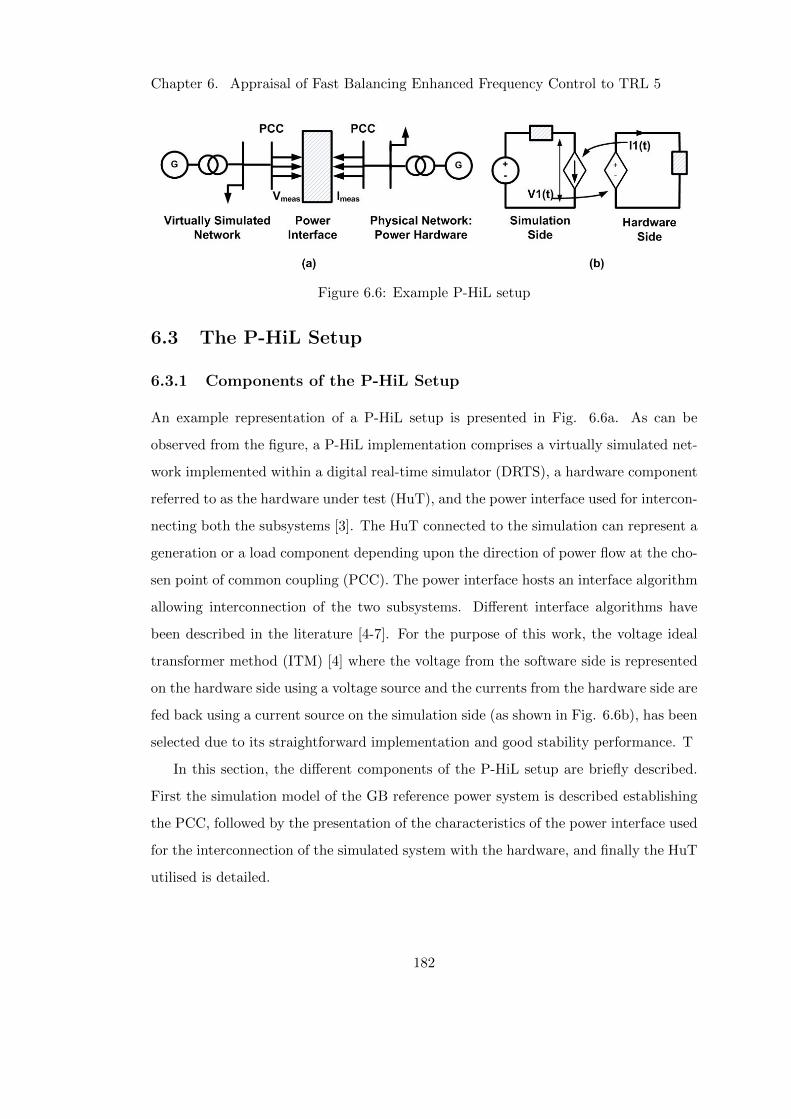
Chapter 6. Appraisal of Fast Balancing Enhanced Frequency Control to TRL 5
Figure 6.6: Example P-HiL setup
6.3 The P-HiL Setup
6.3.1 Components of the P-HiL Setup
An example representation of a P-HiL setup is presented in Fig. 6.6a. As can be
observed from the figure, a P-HiL implementation comprises a virtually simulated net-
work implemented within a digital real-time simulator (DRTS), a hardware component
referred to as the hardware under test (HuT), and the power interface used for intercon-
necting both the subsystems [3]. The HuT connected to the simulation can represent a
generation or a load component depending upon the direction of power flow at the cho-
sen point of common coupling (PCC). The power interface hosts an interface algorithm
allowing interconnection of the two subsystems. Different interface algorithms have
been described in the literature [4-7]. For the purpose of this work, the voltage ideal
transformer method (ITM) [4] where the voltage from the software side is represented
on the hardware side using a voltage source and the currents from the hardware side are
fed back using a current source on the simulation side (as shown in Fig. 6.6b), has been
selected due to its straightforward implementation and good stability performance. T
In this section, the different components of the P-HiL setup are briefly described.
First the simulation model of the GB reference power system is described establishing
the PCC, followed by the presentation of the characteristics of the power interface used
for the interconnection of the simulated system with the hardware, and finally the HuT
utilised is detailed.
182
Chapter 6. Appraisal of Fast Balancing Enhanced Frequency Control to TRL 5
Great Britain Power System
A single line diagram of the reduced five-area GB power system is shown in Fig. 6.7.
The bus wise generation, bus wise active and reactive power load, inter-area power
flows have been presented in Tables 6.3 - 6.7. As can be observed from Fig. 6.7, the
Table 6.3: Bus wise Generation (MVA)
G1 G2 G3 G4 G5 G6
11500 20500 9660 16000 5500 500
Table 6.4: Bus wise Load: Active (MW)
L1 L2 L3 L4 L5 L6
8486 12548 8398 26852 2000 100
Table 6.5: Bus wise Load: Reactive (MVAR)
L1 L2 L3 L4 L5 L6
4109 6077 4067 13005 1041 500
5
G1
G2
G3
G6
G5G4
L1
L2
L3
L4
L6
L5
LFC1
LFC2 LFC3
LFC4
LFC5
Hardware
LFC Areas
Virtual
LFC Areas
Figure 6.7: Five area GB reference power system.
183
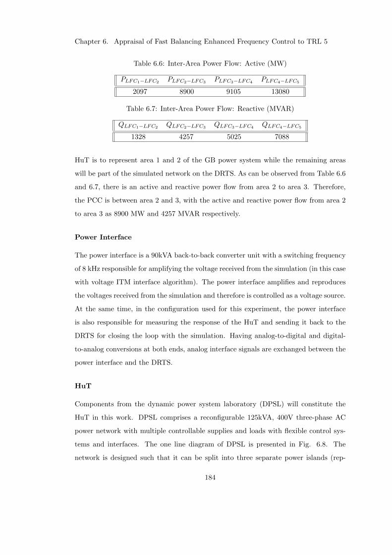
Chapter 6. Appraisal of Fast Balancing Enhanced Frequency Control to TRL 5
Table 6.6: Inter-Area Power Flow: Active (MW)
PLFC1−LFC2 PLFC2−LFC3 PLFC3−LFC4 PLFC4−LFC5
2097 8900 9105 13080
Table 6.7: Inter-Area Power Flow: Reactive (MVAR)
QLFC1−LFC2 QLFC2−LFC3 QLFC3−LFC4 QLFC4−LFC5
1328 4257 5025 7088
HuT is to represent area 1 and 2 of the GB power system while the remaining areas
will be part of the simulated network on the DRTS. As can be observed from Table 6.6
and 6.7, there is an active and reactive power flow from area 2 to area 3. Therefore,
the PCC is between area 2 and 3, with the active and reactive power flow from area 2
to area 3 as 8900 MW and 4257 MVAR respectively.
Power Interface
The power interface is a 90kVA back-to-back converter unit with a switching frequency
of 8 kHz responsible for amplifying the voltage received from the simulation (in this case
with voltage ITM interface algorithm). The power interface amplifies and reproduces
the voltages received from the simulation and therefore is controlled as a voltage source.
At the same time, in the configuration used for this experiment, the power interface
is also responsible for measuring the response of the HuT and sending it back to the
DRTS for closing the loop with the simulation. Having analog-to-digital and digital-
to-analog conversions at both ends, analog interface signals are exchanged between the
power interface and the DRTS.
HuT
Components from the dynamic power system laboratory (DPSL) will constitute the
HuT in this work. DPSL comprises a reconfigurable 125kVA, 400V three-phase AC
power network with multiple controllable supplies and loads with flexible control sys-
tems and interfaces. The one line diagram of DPSL is presented in Fig. 6.8. The
network is designed such that it can be split into three separate power islands (rep-
184
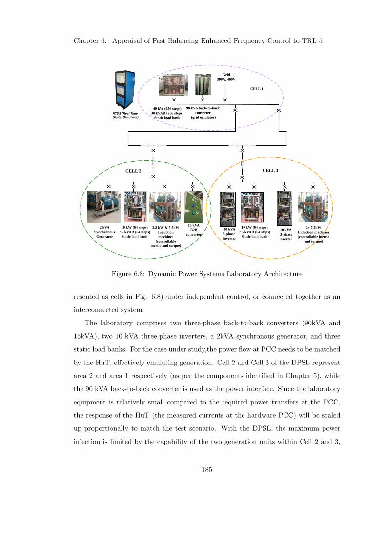
Chapter 6. Appraisal of Fast Balancing Enhanced Frequency Control to TRL 5
RTDS (Real Time
Digital Simulator)
Grid
300A, 400V
90 kVA back-to-back
converter
(grid emulator)
40 kW (256 steps)
30 kVAR (256 steps)
Static load bank
2 kVA
Synchronous
Generator
2x 7.5kW
Induction machines
(controllable inertia
and torque)
10 kVA
3-phase
inverter
2.2 kW & 5.5kW
Induction
machines
(controllable
inertia and torque)
10 kVA
3-phase
inverter
15 kVA
B2B
converter
10 kW (64 steps)
7.5 kVAR (64 steps)
Static load bank
10 kW (64 steps)
7.5 kVAR (64 steps)
Static load bank
CELL 1
CELL 2 CELL 3
Figure 6.8: Dynamic Power Systems Laboratory Architecture
resented as cells in Fig. 6.8) under independent control, or connected together as an
interconnected system.
The laboratory comprises two three-phase back-to-back converters (90kVA and
15kVA), two 10 kVA three-phase inverters, a 2kVA synchronous generator, and three
static load banks. For the case under study,the power flow at PCC needs to be matched
by the HuT, effectively emulating generation. Cell 2 and Cell 3 of the DPSL represent
area 2 and area 1 respectively (as per the components identified in Chapter 5), while
the 90 kVA back-to-back converter is used as the power interface. Since the laboratory
equipment is relatively small compared to the required power transfers at the PCC,
the response of the HuT (the measured currents at the hardware PCC) will be scaled
up proportionally to match the test scenario. With the DPSL, the maximum power
injection is limited by the capability of the two generation units within Cell 2 and 3,
185

Chapter 6. Appraisal of Fast Balancing Enhanced Frequency Control to TRL 5
i.e. 10kVA per cell. In order to represent the 8900MW and 4257MVAR from area 1
and 2, the hardware currents are scaled by means of a scaling factor. For this work the
scaling factor is chosen as k=1x10⁶.
6.3.2 Initialisation and Synchronisation of the P-HiL Setup
The incorporation of the five area GB reference power system within P-HiL setup entails
the representation of a large portion of the test network by HuT. Such a P-HiL setup
has not been reported in literature and presents challenges that need to be addressed.
In the following sub-sections, first the challenge is defined followed by exploring the
options available to address the challenge.
Challenge: A Paradoxical Scenario
The process of setting up a P-HiL simulation involves the following steps:
1. The power network within the DRTS is initialised, allowing for it to attain a
steady state (referred to as initialisation in this work).
2. Interface signals from the initialised DRTS simulation are reproduced by the
power interface.
3. The HuT response to the reproduced signals is measured and fed back to the
DRTS by the power interface to complete the loop (referred to as synchronisation
in this work).
For studies of synchronous power systems, the load and generation conditions along
with the power transfer at selected points of interest are selected from known scenarios.
This allows for testing under known stress conditions of the network or scenarios of
interest (for example, a measured past pre-fault condition of the network, where a
novel control algorithm can be tested in order to analyse if the performance of such
controller can improve the behaviour compared to the former one). Therefore, when
a P-HiL simulation is initialised and synchronised, it is important to ensure that the
conditions at the different buses of the test network are comparable to that of a pure
simulation.
186
Chapter 6. Appraisal of Fast Balancing Enhanced Frequency Control to TRL 5
In most P-HiL applications, the HuT is or represents a relatively small portion of
the network compared to the grid emulation i.e., the rest of the system being simulated
on the DRTS [8-10]. In such cases, the DRTS simulation can be initialised without the
HuT, as the power network within the DRTS is usually a stiff grid whose voltage and
frequency are not dependent upon the HuT to be interconnected. In a similar manner,
the HuT is synchronised with DRTS simulation by means of a simple switch, closing
the loop between HuT and DRTS. Operation of a switch always introduces transient;
however, in cases where the simulated network is a stiff grid or the HuT is a small
network component, this transient does not pose a risk to the stability of the system.
It can therefore be said that the process of initialisation and synchronisation of P-HiL
setup is relatively straightforward.
However, for the case under study, the HuT represents a significant portion of the
test network. In such cases, the initialisation and synchronisation of P-HiL experiment
presents a paradoxical scenario where the DRTS simulation cannot be initialised with-
out the hardware currents, while the hardware currents cannot be produced without
the DRTS simulation being initialised. To elaborate, as the HuT to be connected rep-
resents a large portion of generation of the test network, the DRTS simulation will fail
to initialize due to the lack of generation. Without the DRTS simulation initialised, the
power interface will not be capable of reproducing the interface signals and therefore
the HuT response cannot be synchronised. On the other hand reproducing the interface
signal during the initialisation of DRTS is risky as the signal might not be suitable for
reproduction or may be over the safety limits of the power amplifier and HuT.
A number of studies have investigated the stability of P-HiL simulations [11-13],
where the main findings are related to stability thresholds imposed by the interface
algorithms used for the P-HiL implementation. Improvements to alleviate the identified
stability limitations have been proposed in [14], [15]. However, these studies investigate
the stability of a P-HiL setup, assuming that the initialisation of the P-HiL simulation
sections, virtual and hardware, have been successfully completed independently and
synchronisation by switch is feasible.
In the following sub-sections the options identified for initialisation and synchroni-
187
Chapter 6. Appraisal of Fast Balancing Enhanced Frequency Control to TRL 5
sation of P-HiL simulations, where the HuT represents a larger or significant portion
of the test network such that the conventional approaches can no longer be employed,
are presented. Through a discussion of the the advantages and disadvantages of each
of the options, this sub-section aims to deduce the the best combination to be utilised.
Options for Initialisation of DRTS Simulation
As has been explained, the GB power system within the DRTS fails to initialize due
to a lack generation. Therefore, to allow for the simulation to initialize, an auxiliary
generation can be utilised, and the following four possible options have been identified.
It should be noted that the options presented below are for more generic P-HiL setups
and not limited to the case under study.
Detailed Simulation of HuT: A detailed model of the HuT can be developed as
part of the network for initialising the DRTS simulation. In most cases, a detailed
model would be the best option, however, developing a detailed model of the HuT can
be an arduous task, and considering that the power flows at the PCC are known, much
simpler solutions can be utilised.
AC Voltage Source: Readily available in every power system simulation tool, an
AC voltage source can be utilised to initialize the test network for P-HiL simulation.
However, as the AC voltage source acts as an infinite source, the power flow of the
network at the PCC cannot be controlled. This would lead to, what can be referred to
as, an unsuccessful initialisation as the state of the network is no longer the intended
test scenario, required for comparison of results (with pure simulation results).
Synchronous Generator: A synchronous generator model can control the active
power at its output terminals for emulating the required active power transfers at the
PCC by means of a simple set-point. The reactive power of a synchronous generator is
controlled by controlling the voltage at its terminal (controlling the excitation system).
Either manual tuning of the voltage reference to the exciter or developing a simple PI
control is required to attain the required reactive power flow at the PCC.
188
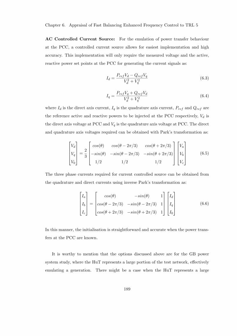
Chapter 6. Appraisal of Fast Balancing Enhanced Frequency Control to TRL 5
AC Controlled Current Source: For the emulation of power transfer behaviour
at the PCC, a controlled current source allows for easiest implementation and high
accuracy. This implementation will only require the measured voltage and the active,
reactive power set points at the PCC for generating the current signals as:
Id =PrefVd −QrefVq
V 2d + V 2
q
(6.3)
Iq =PrefVq +QrefVd
V 2d + V 2
q
(6.4)
where Id is the direct axis current, Iq is the quadrature axis current, Pref and Qref are
the reference active and reactive powers to be injected at the PCC respectively, Vd is
the direct axis voltage at PCC and Vq is the quadrature axis voltage at PCC. The direct
and quadrature axis voltages required can be obtained with Park’s transformation as:
Vd
Vq
V0
=2
3
cos(θ) cos(θ − 2π/3) cos(θ + 2π/3)
−sin(θ) −sin(θ − 2π/3) −sin(θ + 2π/3)
1/2 1/2 1/2
Va
Vb
Vc
(6.5)
The three phase currents required for current controlled source can be obtained from
the quadrature and direct currents using inverse Park’s transformation as:
Ia
Ib
Ic
=
cos(θ) −sin(θ) 1
cos(θ − 2π/3) −sin(θ − 2π/3) 1
cos(θ + 2π/3) −sin(θ + 2π/3) 1
Id
Iq
I0
(6.6)
In this manner, the initialisation is straightforward and accurate when the power trans-
fers at the PCC are known.
It is worthy to mention that the options discussed above are for the GB power
system study, where the HuT represents a large portion of the test network, effectively
emulating a generation. There might be a case when the HuT represents a large
189
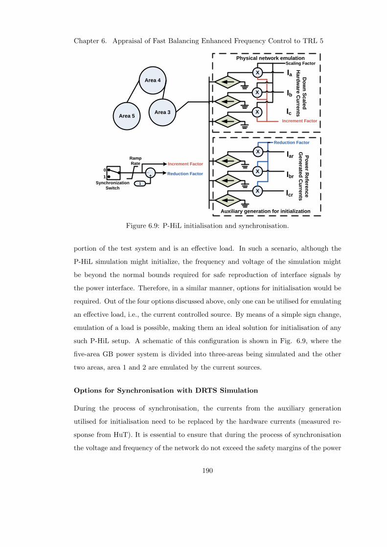
Chapter 6. Appraisal of Fast Balancing Enhanced Frequency Control to TRL 5
Do
wn
Sc
ale
d
Ha
rdw
are
Cu
rren
ts
Ia
Ib
Ic
Area 4
Scaling Factor
Area 5Area 3
Iar
Ibr
Icr
Reduction Factor
Increment Factor
Auxiliary generation for initialization
Synchronization
Switch
0
1
Ramp
Rate
1
_+
Increment Factor
Reduction Factor
Physical network emulation
Po
we
r Re
fere
nc
e
Ge
ne
rate
d C
urre
nts
X
X
X
X
X
X
Figure 6.9: P-HiL initialisation and synchronisation.
portion of the test system and is an effective load. In such a scenario, although the
P-HiL simulation might initialize, the frequency and voltage of the simulation might
be beyond the normal bounds required for safe reproduction of interface signals by
the power interface. Therefore, in a similar manner, options for initialisation would be
required. Out of the four options discussed above, only one can be utilised for emulating
an effective load, i.e., the current controlled source. By means of a simple sign change,
emulation of a load is possible, making them an ideal solution for initialisation of any
such P-HiL setup. A schematic of this configuration is shown in Fig. 6.9, where the
five-area GB power system is divided into three-areas being simulated and the other
two areas, area 1 and 2 are emulated by the current sources.
Options for Synchronisation with DRTS Simulation
During the process of synchronisation, the currents from the auxiliary generation
utilised for initialisation need to be replaced by the hardware currents (measured re-
sponse from HuT). It is essential to ensure that during the process of synchronisation
the voltage and frequency of the network do not exceed the safety margins of the power
190
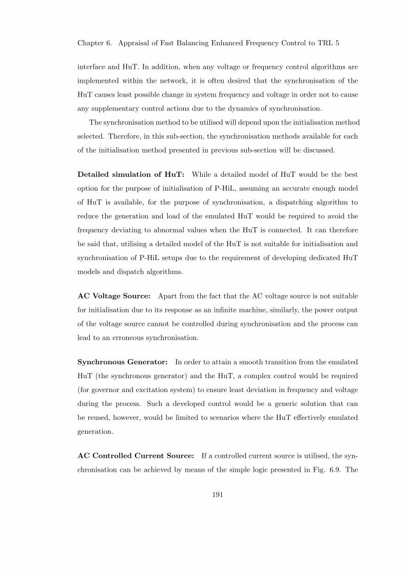
Chapter 6. Appraisal of Fast Balancing Enhanced Frequency Control to TRL 5
interface and HuT. In addition, when any voltage or frequency control algorithms are
implemented within the network, it is often desired that the synchronisation of the
HuT causes least possible change in system frequency and voltage in order not to cause
any supplementary control actions due to the dynamics of synchronisation.
The synchronisation method to be utilised will depend upon the initialisation method
selected. Therefore, in this sub-section, the synchronisation methods available for each
of the initialisation method presented in previous sub-section will be discussed.
Detailed simulation of HuT: While a detailed model of HuT would be the best
option for the purpose of initialisation of P-HiL, assuming an accurate enough model
of HuT is available, for the purpose of synchronisation, a dispatching algorithm to
reduce the generation and load of the emulated HuT would be required to avoid the
frequency deviating to abnormal values when the HuT is connected. It can therefore
be said that, utilising a detailed model of the HuT is not suitable for initialisation and
synchronisation of P-HiL setups due to the requirement of developing dedicated HuT
models and dispatch algorithms.
AC Voltage Source: Apart from the fact that the AC voltage source is not suitable
for initialisation due to its response as an infinite machine, similarly, the power output
of the voltage source cannot be controlled during synchronisation and the process can
lead to an erroneous synchronisation.
Synchronous Generator: In order to attain a smooth transition from the emulated
HuT (the synchronous generator) and the HuT, a complex control would be required
(for governor and excitation system) to ensure least deviation in frequency and voltage
during the process. Such a developed control would be a generic solution that can
be reused, however, would be limited to scenarios where the HuT effectively emulated
generation.
AC Controlled Current Source: If a controlled current source is utilised, the syn-
chronisation can be achieved by means of the simple logic presented in Fig. 6.9. The
191

Chapter 6. Appraisal of Fast Balancing Enhanced Frequency Control to TRL 5
synchronisation process is begun by means of a synchronisation switch that inversely
ramps up and down both controlled current sources. The ramp rate can be chosen such
that it does not create any oscillations or transients on the system. Once the currents
from the auxiliary generation are reduced to zero and the currents from the HuT are
fully connected to the simulation, the system is synchronised.
From the above discussion, it can be deduced that for the purpose of initialisation
and synchronisation of P-HiL setups, where the HuT represents a large portion of the
test network, the most convenient option available is to utilize a controlled current
source. A controlled current source offers the easiest implementation, is very accurate
while at the same time a generic approach that can be utilised when the HuT emulates
a generation or a load.
6.3.3 Accuracy of the P-HiL Setup
Once a P-HiL has been successfully initialised and synchronised, an important aspect
of any P-HiL setup is to ensure its accuracy before any tests are undertaken. In any
P-HiL setup, it can be observed that the power exchange at the physical PCC does not
match the power exchange at the virtual PCC, i.e. although accurate power is being
injected/drawn by the HuT at the physical PCC, the PCC within the DRTS simulation
presents a different power factor. This behaviour can be attributed to the time delay
of the entire P-HiL process: the processing time of the DRTS, the communication
between DRTS and power interface, the power interface processing time for amplifying
the signal and the feedback loop measurement and communication. This time delay
presents itself as an additional phase difference between voltage and current. The added
phase difference between voltage and current at the simulation PCC, affects the power
factor of the HuT, leading to inaccurate active and reactive power exchanges compared
to an ideal scenario.
The impact of time delay on the accuracy of simulations has been extensively evalu-
ated and the need for compensating the delay emphasised in [16-18]. If these delays are
not appropriately compensated, it is not possible to ensure the equality of the reference
192
Chapter 6. Appraisal of Fast Balancing Enhanced Frequency Control to TRL 5
Figure 6.10: Time delay compensation method employed [22].
power and the injected power and therefore the fidelity of the simulation. A number
of methods have been reported in literature to compensate for the delays encountered
while closing the loop in a P-HiL setup [19-21]. For this work, a phase compensation
method, as reported in [22], is utilised. The time delay of an AC signal is equivalent
to a phase shift in the frequency domain, the method proposed to compensate for the
time delay (as shown in Fig. 6.10) decomposes the signal from the DRTS with an
FFT transforming the time domain signal into the frequency domain. In the frequency
domain, additional phase is added to the fundamental and harmonics analysed to com-
pensate for the time delay of the system. After the compensation takes place, the signal
is reconstructed and can be accurately amplified by the power interface. For a specific
implementation, this delay can be treated as approximately constant and deterministic,
although this should be assessed on a case by case basis.
6.3.4 Initialisation and Synchronisation Results
A schematic of the P-HiL interconnection within RSCAD has been shown in Fig. 6.9.
An auxiliary generation (the controlled current source in this case) is utilised to re-
produce currents generated from the power reference i.e. 8900MW and 4257MVAR,
initialising the real time simulation. Once the simulation has initialised and attained a
steady state, the PCC voltages are reproduced using the power interface. The measured
HuT currents should be equal (as much as possible) to the emulated HuT currents. In
193
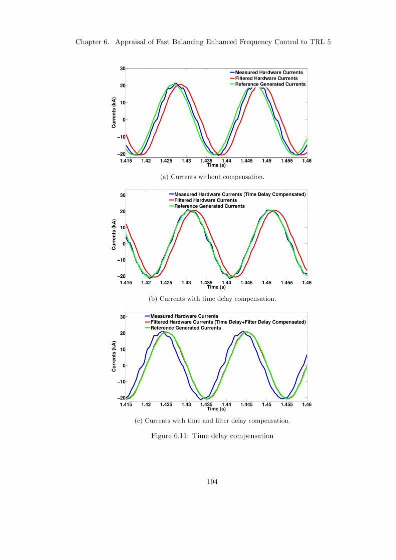
Chapter 6. Appraisal of Fast Balancing Enhanced Frequency Control to TRL 5
1.415 1.42 1.425 1.43 1.435 1.44 1.445 1.45 1.455 1.46
−20
−10
0
10
20
30
Time (s)
Cu
rren
ts (
kA
)
Measured Hardware Currents
Filtered Hardware Currents
Reference Generated Currents
(a) Currents without compensation.
1.415 1.42 1.425 1.43 1.435 1.44 1.445 1.45 1.455 1.46
−20
−10
0
10
20
30
Time (s)
Cu
rren
ts (
kA
)
Measured Hardware Currents (Time Delay Compensated)
Filtered Hardware Currents
Reference Generated Currents
(b) Currents with time delay compensation.
1.415 1.42 1.425 1.43 1.435 1.44 1.445 1.45 1.455 1.46
−20
−10
0
10
20
30
Time (s)
Cu
rren
ts (
kA
)
Measured Hardware Currents
Filtered Hardware Currents (Time Delay+Filter Delay Compensated)
Reference Generated Currents
(c) Currents with time and filter delay compensation.
Figure 6.11: Time delay compensation
194
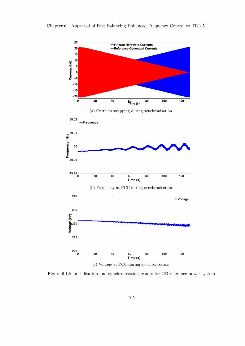
Chapter 6. Appraisal of Fast Balancing Enhanced Frequency Control to TRL 5
0 20 40 60 80 100 120
−20
−15
−10
−5
0
5
10
15
20
25
Time (s)
Cu
rren
ts (
kA
)
Filtered Hardware Currents
Reference Generated Currents
(a) Currents swapping during synchronisation.
0 20 40 60 80 100 120
Time (s)
49.98
49.99
50
50.01
50.02
Fre
qu
en
cy (
Hz)
Frequency
(b) Frequency at PCC during synchronisation.
0 20 40 60 80 100 120
Time (s)
220
225
230
235
240
Vo
ltag
e (
kV
)
Voltage
(c) Voltage at PCC during synchronisation.
Figure 6.12: Initialisation and synchronisation results for GB reference power system
195
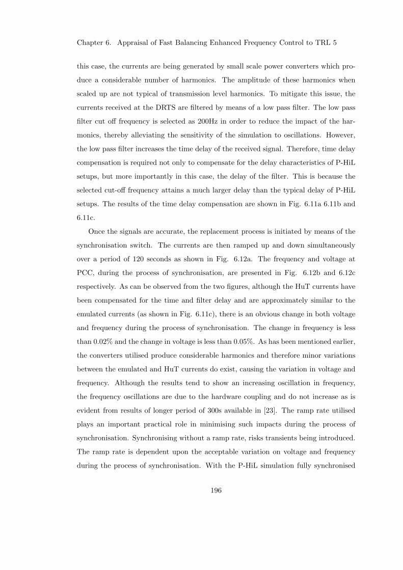
Chapter 6. Appraisal of Fast Balancing Enhanced Frequency Control to TRL 5
this case, the currents are being generated by small scale power converters which pro-
duce a considerable number of harmonics. The amplitude of these harmonics when
scaled up are not typical of transmission level harmonics. To mitigate this issue, the
currents received at the DRTS are filtered by means of a low pass filter. The low pass
filter cut off frequency is selected as 200Hz in order to reduce the impact of the har-
monics, thereby alleviating the sensitivity of the simulation to oscillations. However,
the low pass filter increases the time delay of the received signal. Therefore, time delay
compensation is required not only to compensate for the delay characteristics of P-HiL
setups, but more importantly in this case, the delay of the filter. This is because the
selected cut-off frequency attains a much larger delay than the typical delay of P-HiL
setups. The results of the time delay compensation are shown in Fig. 6.11a 6.11b and
6.11c.
Once the signals are accurate, the replacement process is initiated by means of the
synchronisation switch. The currents are then ramped up and down simultaneously
over a period of 120 seconds as shown in Fig. 6.12a. The frequency and voltage at
PCC, during the process of synchronisation, are presented in Fig. 6.12b and 6.12c
respectively. As can be observed from the two figures, although the HuT currents have
been compensated for the time and filter delay and are approximately similar to the
emulated currents (as shown in Fig. 6.11c), there is an obvious change in both voltage
and frequency during the process of synchronisation. The change in frequency is less
than 0.02% and the change in voltage is less than 0.05%. As has been mentioned earlier,
the converters utilised produce considerable harmonics and therefore minor variations
between the emulated and HuT currents do exist, causing the variation in voltage and
frequency. Although the results tend to show an increasing oscillation in frequency,
the frequency oscillations are due to the hardware coupling and do not increase as is
evident from results of longer period of 300s available in [23]. The ramp rate utilised
plays an important practical role in minimising such impacts during the process of
synchronisation. Synchronising without a ramp rate, risks transients being introduced.
The ramp rate is dependent upon the acceptable variation on voltage and frequency
during the process of synchronisation. With the P-HiL simulation fully synchronised
196
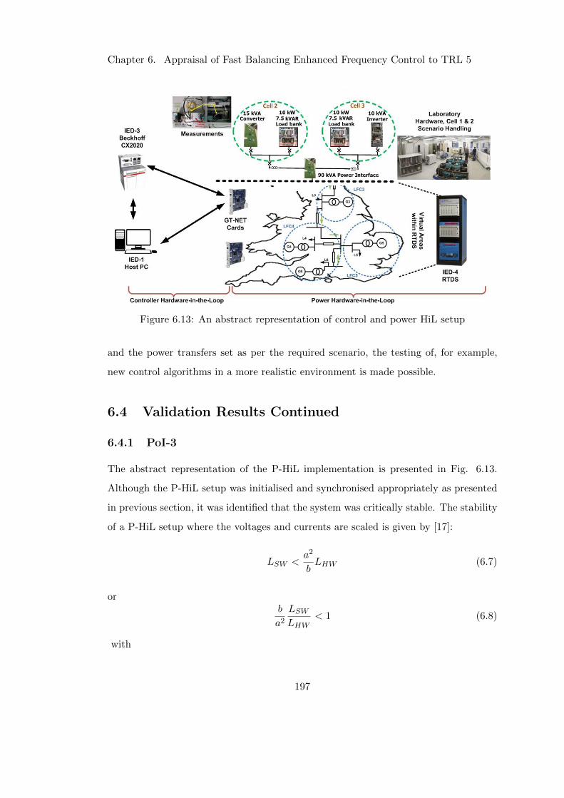
Chapter 6. Appraisal of Fast Balancing Enhanced Frequency Control to TRL 5
Figure 6.13: An abstract representation of control and power HiL setup
and the power transfers set as per the required scenario, the testing of, for example,
new control algorithms in a more realistic environment is made possible.
6.4 Validation Results Continued
6.4.1 PoI-3
The abstract representation of the P-HiL implementation is presented in Fig. 6.13.
Although the P-HiL setup was initialised and synchronised appropriately as presented
in previous section, it was identified that the system was critically stable. The stability
of a P-HiL setup where the voltages and currents are scaled is given by [17]:
LSW <a2
bLHW (6.7)
orb
a2LSWLHW
< 1 (6.8)
with
197

Chapter 6. Appraisal of Fast Balancing Enhanced Frequency Control to TRL 5
a =VSWVHW
(6.9)
b =IHuTfullIHuTred
(6.10)
where LSW is the software side inductance, LHW is the hardware side inductance, VSW ,
VHW are the phase nominal voltages of the software and hardware side respectively,
IHuTfull , IHuTred are the nominal current of the full-scale HuT and the reduced-scale
HuT respectively. For the study under consideration,
a =VSWVHW
=400kV
400V= 1× 10³ (6.11)
b =IHuTfullIHuTred
= 1× 10⁶ (6.12)
b
a2= 1 (6.13)
LSWLHW
' 1 (6.14)
with the given values, as can be observed, the condition for stability is met, however,
any small change can lead the system to instability. To allow for a safety margin,
the value of IHuTred is increased such that b = 0.8. As the currents from hardware
units needed to be increased, this limits the spare power capacity that was reserved
for reference imbalance event. For this reason, the value of imbalance event in this
case is reduced to 800MW (maximum) represented by 1000W in hardware. This would
suffice to achieve the objective of PoI-3, i.e., to test the ability of the control with real
measurements.
The system is subject to two disturbances in LFC 2 (Cell 2 in hardware, Fig.
6.8), a loss of generation and a loss of load, with magnitudes of 800MW (1000kW in
hardware) and 700MW (875W in hardware) respectively. The parameters of the control
system remain same as in the previous study. The system frequency response subject
to generation loss and load loss at t = 10s are presented in Fig. 6.14 (superimposed).
As can be observed, the EFC-FB was able to identify the imbalance evident from the
restoration of frequency much faster than conventional LFC framework.
198
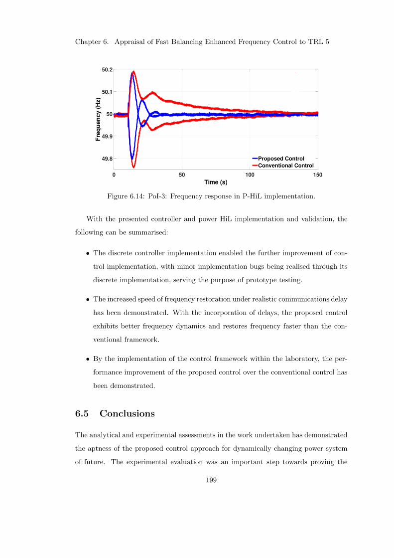
Chapter 6. Appraisal of Fast Balancing Enhanced Frequency Control to TRL 5
0 50 100 150
Time (s)
49.8
49.9
50
50.1
50.2
Fre
qu
en
cy (
Hz)
Proposed Control
Conventional Control
Figure 6.14: PoI-3: Frequency response in P-HiL implementation.
With the presented controller and power HiL implementation and validation, the
following can be summarised:
• The discrete controller implementation enabled the further improvement of con-
trol implementation, with minor implementation bugs being realised through its
discrete implementation, serving the purpose of prototype testing.
• The increased speed of frequency restoration under realistic communications delay
has been demonstrated. With the incorporation of delays, the proposed control
exhibits better frequency dynamics and restores frequency faster than the con-
ventional framework.
• By the implementation of the control framework within the laboratory, the per-
formance improvement of the proposed control over the conventional control has
been demonstrated.
6.5 Conclusions
The analytical and experimental assessments in the work undertaken has demonstrated
the aptness of the proposed control approach for dynamically changing power system
of future. The experimental evaluation was an important step towards proving the
199

Chapter 6. Appraisal of Fast Balancing Enhanced Frequency Control to TRL 5
ability of the proposed controls to perform under real-world conditions. While the
simulations already highlighted the benefits of these controls over state-of-the-art, it
remained unclear whether the new approach would perform satisfactorily outside ide-
alised simulated conditions. Therefore, the conducted experiments where imperative
to highlight the real-world applicability of the proposed control. The resilience of the
proposed controller to communications asynchronicity, finite measurement and control
step resolution, various noise sources, parameter uncertainties, and other factors not ex-
plicitly incorporated in the mathematical model were tested in the process as well. The
deployment of the control on dedicated controller hardware enabled rapid prototyping,
allowing for an efficient iterative development process by feeding back experiences made
under real conditions into the theoretical method.
With the development of the EFC and its validation in a laboratory environment,
the ability of more decentralised and distributed operation of power system has been
proven. Furthermore, the developed control, in essence works towards the objective
of solving local problems locally. Beginning with the speculation of advantages of
more local control, this exercise has proven some merits of prioritising of local response
to a local imbalance, such as improved dynamic response, robust reserve activations
and reducing the divergence from planned system conditions and hence minimising the
operational implications of the disturbance. In addition, the developed controls support
enhanced scalability in the future grid given the autonomy of the approaches.
200
Chapter 6. Appraisal of Fast Balancing Enhanced Frequency Control to TRL 5
REFERENCES
[1] M. H. Syed, G.M. Burt, R. D’Hulst, and J. Verbeeck,“Experimental Validation
of Flexibility Provision by Highly Distributed Demand Portfolio”, in proceedings
of the 2016 CIRED Workshop, pp. 1-4, Helsinki, Finland, 2016.
[2] P. Dambrauskas, M. H. Syed, S. M. Blair, J. M. Irvine, I. F. Abdulhadi, G. M.
Burt, and D. E. M. Bondy ”Impact of realistic communications for fast-acting
demand side management,” in CIRED - Open Access Proceedings Journal, vol.
2017, no. 1, pp. 1813-1817, 10 2017.
[3] G. F. Lauss, M. O. Faruque, K. Schoder, C. Dufour, A. Viehweider, and J.
Langston, “Characteristics and Design of Power Hardware-in-the-Loop Simula-
tions for Electrical Power Systems”, in IEEE Trans. on Industrial Electronics,
vol. 63, no. 1, pp. 406-417, Jan. 2016.
[4] W. Ren, M. Steurer, and T. L. Baldwin, “Improve the Stability and the Accuracy
of Power Hardware-in-the-Loop Simulation by Selecting Appropriate Interface
Algorithms”, in IEEE Trans. on Industry Applications, vol. 44, no. 4, pp. 1286-
1294, July 2008.
[5] F. Lehfuss, G. Lauss, and T. Strasser, “Implementation of a multi-rating inter-
face for Power-Hardware-in-the-Loop simulations”, in proceedings of 2012 38ˆth
Annual Conference on IEEE Industrial Electronics Society (IECON), Montreal,
QC, pp. 4777-4782, 2012.
[6] S. Lentijo, S. D’Arco, and A. Monti, “Comparing the Dynamic Performances of
Power Hardware-in-the-Loop Interfaces”, in IEEE Trans. on Industrial Electron-
ics, vol. 57, no. 4, pp. 1195-1207, April 2010.
[7] E. Jong, R. de Graaff, P. Vaessen, P. Crolla, A. J. Roscoe, F. Lefuss, G. Lauss,
P. Kotsampopoulos, and F. Gafaro, “European White Book on Real-Time Power
Hardware in the Loop Testing”, DERlab, 2012.
201
Chapter 6. Appraisal of Fast Balancing Enhanced Frequency Control to TRL 5
[8] J. Langston, K. Schoder, M. Steurer, O. Faruque, J. Hauer, F. Bogdan, R. Bravo,
B. Mather, and F. Katiraei, “Power hardware-in-the-loop testing of a 500 kW
photovoltaic array inverter”, in proceedings of 2012 38ˆth Annual Conference on
IEEE Industrial Electronics Society (IECON), Montreal, QC, pp. 4797-4802,
2012.
[9] O. Naeckel, J. Langston, M. Steurer, F. Fleming, S. Paran, C. Edrington, and M.
Noe, “Power Hardware-in-the-Loop Testing of an Air Coil Superconducting Fault
Current Limiter Demonstrator”, in IEEE Trans. on Applied Superconductivity,
vol. 25, no. 3, pp. 1-7, June 2015.
[10] P. Kotsampopoulos, N. Hatziargyriou, B. Bletterie, G. Lauss, and T. Strasser,
“Introduction of advanced testing procedures including PHIL for DG providing
ancillary services”, in proceedings of the 39ˆth Annual Conference of the IEEE
Industrial Electronics Society (IECON), Vienna, pp. 5398-5404, 2013.
[11] A. Viehweider, G. Lauss, and F. Lehfuss, “Stabilization of Power Hardware-in-
the-Loop Simulations of Electric Energy Systems”, Simulation Modelling Practice
and Theory, vol.19, no.7, pp. 1699-1708, 2011.
[12] T. Hatakeyama, A. Riccobono, and A. Monti, “Stability and accuracy analysis
of power hardware in the loop system with different interface algorithms”, in
proceedings of the 2016 IEEE 17ˆth Workshop on Control and Modeling for Power
Electronics (COMPEL), Trondheim, pp. 1-8, 2016.
[13] M. Dargahi, A. Ghosh, and G. Ledwich, “Stability synthesis of power hardware-in-
the-loop (PHIL) simulation”, in proceedings of the 2014 IEEE Power and Energy
Society General Meeting - Conference & Exposition, National Harbor, MD, pp.
1-5, 2014.
[14] E. Liegmann, A. Riccobono, and A. Monti, “Wideband identification of impedance
to improve accuracy and stability of power-hardware-in-the-loop simulations”, in
proceeding of the 2016 IEEE International Workshop on Applied Measurements
for Power Systems (AMPS), Aachen, pp. 1-6, 2016.
202
Chapter 6. Appraisal of Fast Balancing Enhanced Frequency Control to TRL 5
[15] R. Brandl, ‘’‘Operational Range of Several Interface Algorithms for Different
Power Hardware-In-The-Loop Setups”,in Energies, 10, 1946, 2017.
[16] F. Huerta, R. L. Tello, and M. Prodanovic, “Real-Time Power-Hardwarein-the-
Loop Implementation of Variable-Speed Wind Turbines”, in IEEE Trans. on
Industrial Electronics, vol. 64, no. 3, pp. 1893–1904, 2017.
[17] I. D. Yoo, and A. M. Gole, “Compensating for interface equipment limitations to
improve simulation accuracy of real-time power hardware in loop simulation”, in
IEEE Trans. on Power Delivery, vol. 27, no. 3, pp. 1284–1291, 2012.
[18] W. Ren, “Accuracy evaluation of power hardware-in-the-loop (PHIL) simulation”,
Ph.D. dissertation, The Florida State University, 2007.
[19] P. C. Kotsampopoulos, F. Lehfuss, G. F. Lauss, B. Bletterie, and N. D. Hatziar-
gyriou, “The limitations of digital simulation and the advantages of PHIL testing
in studying distributed generation provision of ancillary services”, in IEEE Trans.
on Industrial Electronics, vol. 62, no. 9, pp. 5502–5515, 2015.
[20] P. Kotsampopoulos, V. Kleftakis, G. Messinis, and N. Hatziargyriou, “Design,
development and operation of a PHIL environment for Distributed Energy Re-
sources”, in Proceedings of Industrial Electronics Conference (IECON), pp. 4765–4770,
2012.
[21] N. Ainsworth, A. Hariri, K. Prabakar, A. Pratt, and M. Baggu, “Modeling and
compensation design for a power hardware-in-the-loop simulation of an AC distri-
bution system”, in proceedings of the NAPS 2016 - 48th North American Power
Symposium, 2016.
[22] E. Guillo-Sansano, A. J. Roscoe, and G. M. Burt, “Harmonic-by-harmonic time
delay compensation method for PHIL simulation of low impedance power sys-
tems”, in proceedings of the 2015 International Symposium on Smart Electric
Distribution Systems and Technologies (EDST), Vienna, pp. 560-565, 2015.
203

Chapter 6. Appraisal of Fast Balancing Enhanced Frequency Control to TRL 5
[23] E. Guillo-Sansano, M. H. Syed, A. J. Roscoe, and G. M. Burt, “Initialization and
Synchronization of Power Hardware-in-the-Loop Simulations: A Great Britain
Network Case Study”, in Energies, vol 11, no. 5, 1087, April 2018.
204

Chapter 7
Conclusions and Future Work
7.1 Summary
With the changes the power systems around the world are expected to undergo in the
near future, the conventional approaches to frequency control ancillary service provi-
sion are being challenged. The need for new services to ensure security of supply has
been established in literature. To this end, this thesis presents two novel frequency
control approaches: (i) a secondary frequency control (SFC) referred to as fast bal-
ancing enhanced frequency control (EFC-FB), and (ii) a primary frequency control
(PFC) referred to as responsibilising primary enhanced frequency control (EFC-RP).
The proposed controls are enabled by effective event detection techniques developed.
The performance of the proposed controls has been verified by real-time simulations
conducted on a validated reduced dynamic model of the Great Britain (GB) power sys-
tem. With the objective of appraising the proposed EFC-FB framework to technology
readiness level (TRL) 5, this thesis further presents a novel methodology to facilitate
laboratory validations of smart grid control solutions.
The following sections outline the major conclusions of this research and identify
areas of research worth being taken forward as future work.
205
Chapter 7. Conclusions and Future Work
7.2 Conclusions
The contributions from the work undertaken throughout this thesis can be attributed
to three distinct knowledge streams. The following three sub-sections present the con-
tributions to each stream in detail.
7.2.1 Enhanced Frequency Control Approaches
Acknowledging the recently identified importance of locational information in addition
to temporal information in effective provision of ancillary services, this thesis intro-
duces the term “responsibilisation” that refers to the prioritisation of remedial control
measures closer to source of an imbalance, thereby supporting the drive towards greater
decentralisation of power systems. To this end, two responsibilising frequency control
ancillary services were proposed. The two control approaches ensure the prioritisation
of local response to a local imbalance, reducing the divergence from planned system
conditions, thereby minimising the operational implications of any system imbalance
event. In addition, they support enhanced scalability in the future grid given the rel-
ative autonomy of the approaches. Each of the following sub-sections will detail the
conclusions of each proposed control.
Fast Balancing Enhanced Frequency Control
The incorporation of conventional Load Frequency Control (LFC) framework within a
validated reduced dynamic model of GB grid, a first implementation of its kind, was
a first step towards increased decentralisation and responsibilisation, where remedial
control measures are taken closer to the location of the imbalance event, i.e. within the
area of the disturbance as opposed to the current practice within GB grid where the
response is from across the country. The GB grid, with conventional LFC framework
incorporated, when subjected to reference imbalance event presented a satisfactory
frequency response. As is well established, responsibilisation within conventional LFC
framework is inherent, therefore the focus was directed towards improving the response
speed.
206
Chapter 7. Conclusions and Future Work
An analysis of the conventional LFC framework response revealed the conflicting
nature of the two objectives, the enhanced responsibilisation and improved response
speed. Increasing the response speed of conventional LFC lead to degradation in re-
sponsibilisation. Further analysis identified limitations within the conventional LFC
framework as a cause for the two objectives to project conflict. These limitations were
identified as:
• The inability of the conventional LFC framework to ascertain definitive location
of the imbalance event.
• The use of a common control effort for slower and faster acting resources.
To overcome the limitations identified, a novel EFC-FB is proposed. The proposed
control incorporates a fast acting balance control loop (BCL), in addition to the sec-
ondary control loop (SCL). The BCL comprises an area disturbance observer, capable
of fast, autonomous and definitive identification of imbalance event location. The con-
trol effort to fast acting resources is a combination of effort from BCL and SCL, while
the control effort to slower acting resources is from SCL only, thereby decoupling the
two. Addressing the limitations allows for unilateral activation of reserves only within
the area where the imbalance event initiated even with faster response speeds. Further-
more, the definitive identification of imbalance location enables the use of direct power
imbalance observed over area tie-lines to be utilised as control input, that is shown to
avoid sympathetic activations at faster response speeds contrary to the conventionally
utilised area control error.
The performance of the proposed control framework is verified by means of real-
time simulations and small-signal analysis conducted on the reduced dynamic model of
GB, before its implementation within the Dynamic Power Systems Laboratory (DPSL)
for its appraisal to TRL 5. Controller hardware in the loop validation revealed issues
in the implementation of the algorithm that were masked by small computational time
step of real-time simulations. This highlights the importance of each stage of the val-
idation chain and further reveals the limitation of pure simulation based approaches.
These issues were addressed before the combined controller and power hardware in
207

Chapter 7. Conclusions and Future Work
the loop validation. The ability of the proposed framework to operate in real-world
conditions, with actual measurements and communication delays, was proven, provid-
ing high degree of confidence in the credibility of the proposed control for real world
implementation.
In essence it can be said that the proposed EFC-FB enables improved response
speeds while at the same time not only ensuring effective, but also enhanced responsi-
bilisation.
Responsibilising Primary Enhanced Frequency Control
Responsibilisation within PFC can be introduced by means of adapting the droop
slopes of the LFC areas in real-time, if the location of the imbalance event can be de-
tected within the timescale of PFC. The disturbance observer of the EFC-FB developed
within this work could be utilised for the purpose of incorporating responsibilisation
within PFC. The disturbance observer approach for event detection is much more ro-
bust compared to alternatives but still not appropriate to be utilised for PFC due to
its centralised event detection as reported in Chapter 4.
Therefore, a novel decentralised responsibilising PFC has been proposed. The con-
trol achieves responsibilisation by means of fast and autonomous event detection and
droop adaptation of LFC areas in real-time. The fast and autonomous event detec-
tion is achieved by means of calculating the transient phase offset (TPO) locally at
resources participating in PFC, while the droop of LFC areas are adapted based on a
droop curve proposed. The proposed approach is fully decentralised as it relies on local
measurement only and requires no form of communication.
Real-time simulation results have shown that an event can effectively be identified
within 100ms of its occurrence and the proposed droop curve enables effective respon-
sibilisation. The linear droop curve proposed in this work serves as a proof of concept.
More sophisticated droop curves can be designed to achieve more effective responsibili-
sation. This has not been explored within this work. The applicability and soundness of
the proposed approach to be operated in conjunction with SFC has been demonstrated
by means of small-signal analysis.
208
Chapter 7. Conclusions and Future Work
7.2.2 Methodology to Facilitate Laboratory Validation of Complex
Smart Grid Control Solutions
The practical challenges that arise from the integration of control solutions within
laboratory environments, for their validation, are identified. These practical challenges
have been given little or no attention in the past, however, with increasing recognition
of laboratory validations, this is the first attempt at reporting these challenges. The
challenges identified were correlated to a lack of an integrated methodology. To address
this issue of lack of an integrated methodology, an approach that utilizes SGAM as a
tool to facilitate laboratory validations is proposed. The proposed methodology leads
to a combined representation of control solutions and laboratory infrastructure, in
other words a comprehensive validation environment, using the SGAM, facilitating the
transition from the design of radical grid control solutions, to their rigorous validation.
The proposed SGAM modelling approach was utilised to develop the validation en-
vironment for the EFC framework. Through a qualitative assessment the competence
of the proposed approach to: (i) entail efficiency in the process of control solution vali-
dation, (ii) incorporate a variety of non-monolithic validation setups and (iii) enhance
repeatability and reproducibility of control solution validations, was established. This
included the adoption of the approach in an independent smart grid laboratory (at
Centre for Renewable Sources and Savings in Greece) to develop a tailored validation
environment for the EFC-FB.
For the first time, two state-of-the-art smart grid laboratories were represented
using SGAM. The representation of two state-of-the-art smart grid laboratories using
SGAM presented an effective means to communicate research infrastructure features
for the integration and validation of complex smart grid control solutions.
The conventional SGAM modelling approach is limited to representation of control
solutions implemented within a single entity (for example, one DSO or TSO). This
presents a limitation on the control solutions that can be represented using SGAM. This
work further introduced a concept to represent a control solution implemented within
more than one entity. This enables representation of distributed control solutions in
SGAM broadening the conventional bounds of SGAM.
209
Chapter 7. Conclusions and Future Work
7.2.3 Extending the Boundaries of Real-Time Power Hardware-in-
the-Loop Simulations
For the first time, the process of initialisation and synchronisation of a power hard-
ware in the loop (P-HiL) setup, wherein the hardware under test (HuT) represents a
significant portion of the network compared to the rest of the system being simulated
within the digital real-time simulator (DRTS), has been demonstrated by means of
implementation within the DPSL.
The initialisation and synchronisation of such setups present challenges such as the
paradoxical scenario explained in detail in Chapter 6. This thesis presents a range
of possible methodologies for improving the initialisation and synchronisation of such
scenarios. The investigation of these alternatives has led to the identification of a
recommended approach that uses current sources for initialisation and symmetrical
ramping rates for synchronisation of the P-HiL simulation with the hardware under
test.
The options available for initialisation and synchronisation of such P-HiL setups
are discussed and the best practices drawn. Furthermore, an additional scenarios that
would transgress from the traditional bounds of P-HiL techniques is identified. The
resulting improved performance and extended range of feasible scenarios that can be
studied have been validated by experimentation of frequency control scenarios for the
GB system. This will allow for safer and more stable P-HiL simulations, and permit
validation of a wider range of realistic simulations through P-HiL to the betterment of
new controllers and power components.
7.3 Future Work
In this section, based on the findings and conclusions of the work undertaken, areas of
future work have been identified and presented in the following sub-sections.
210
Chapter 7. Conclusions and Future Work
7.3.1 Enhanced Frequency Control Architecture for Future Power
Systems
In this work, the two novel frequency control solutions for greater decentralisation and
distributed operation of future power systems were developed. The following can be
deduced:
• The two controls were developed independently.
• The traditional definitions used for frequency control are being challenged, the
line between the primary frequency control and secondary frequency control is
becoming more blurred.
• The TPO based method holds greater potential.
Therefore, the future work involves the development of a novel frequency control ar-
chitecture that incorporates the TPO based disturbance detection for both frequency
containment and restoration.
7.3.2 Refinement of Laboratory Validation Approach
The SGAM based modelling approach for laboratory validation of smart grid control
solutions proposed in this work has proven to be advantageous. The methodology
was adopted for laboratory validation of EFC framework proposed within this work
by two independent laboratories. However, the methodology was confined to in-house
developed control solution. The future work involves the use of the methodology for
wide range of smart grid control solutions, in particular control solutions developed
by third party, and to spread the use of the methodology to more laboratories across
Europe. This will allow for feedback to be gathered and to identify the potential areas
for further refinement of the proposed approach.
211
Chapter 7. Conclusions and Future Work
7.3.3 Improving Real-Time Simulations for Extending Laboratory Val-
idations
The traditional P-HiL methods are being challenged by the need for expanding its
envelope to validate larger power networks in larger P-HiL setups. An example of such
is, the additional scenario identified within this thesis, of a power system incorporating
high penetration of converter based generation and/or wide area monitoring control
solutions. Such setups present a number of challenges in terms of the protection and
stability of P-HiL. This again presents an excellent direction that is worthy of further
exploration.
7.3.4 Monetisation of Developed Frequency Control Approaches
The monetisation and incorporation within the market of novel frequency support ap-
proaches such as those proposed in this work is an important aspect that remains
to be investigated. Although it is intuitive that the change in market design is in-
evitable, driven by the need of the power system, it is important to understand how
the responsibilising controls will be regulated to ensure fairness. It is assumed that re-
sponsibilisation would prevent wider system participation (as is its objective), thereby
causing monetary hotspots in the network where participants stand to gain more profits
than resources elsewhere in the network. An analysis of the impact of responsibilisation
on market regulations and framework is an area that deserves more attention.
212

Appendices
213
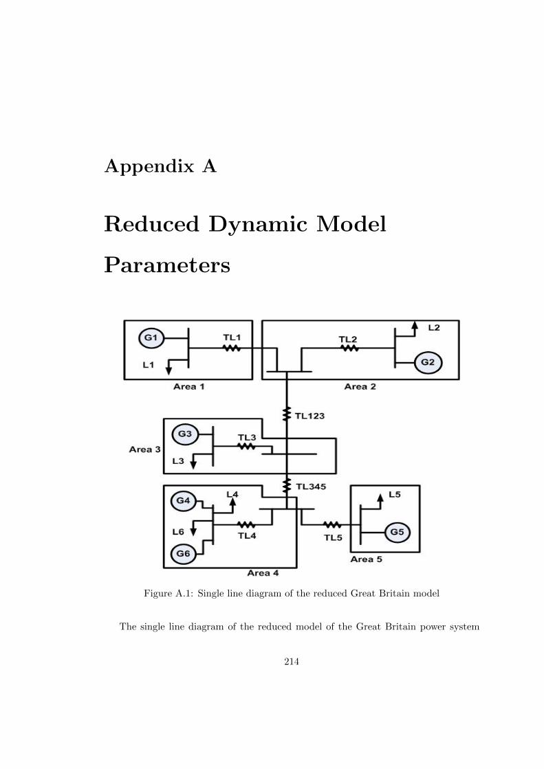
Appendix A
Reduced Dynamic Model
Parameters
Figure A.1: Single line diagram of the reduced Great Britain model
The single line diagram of the reduced model of the Great Britain power system
214
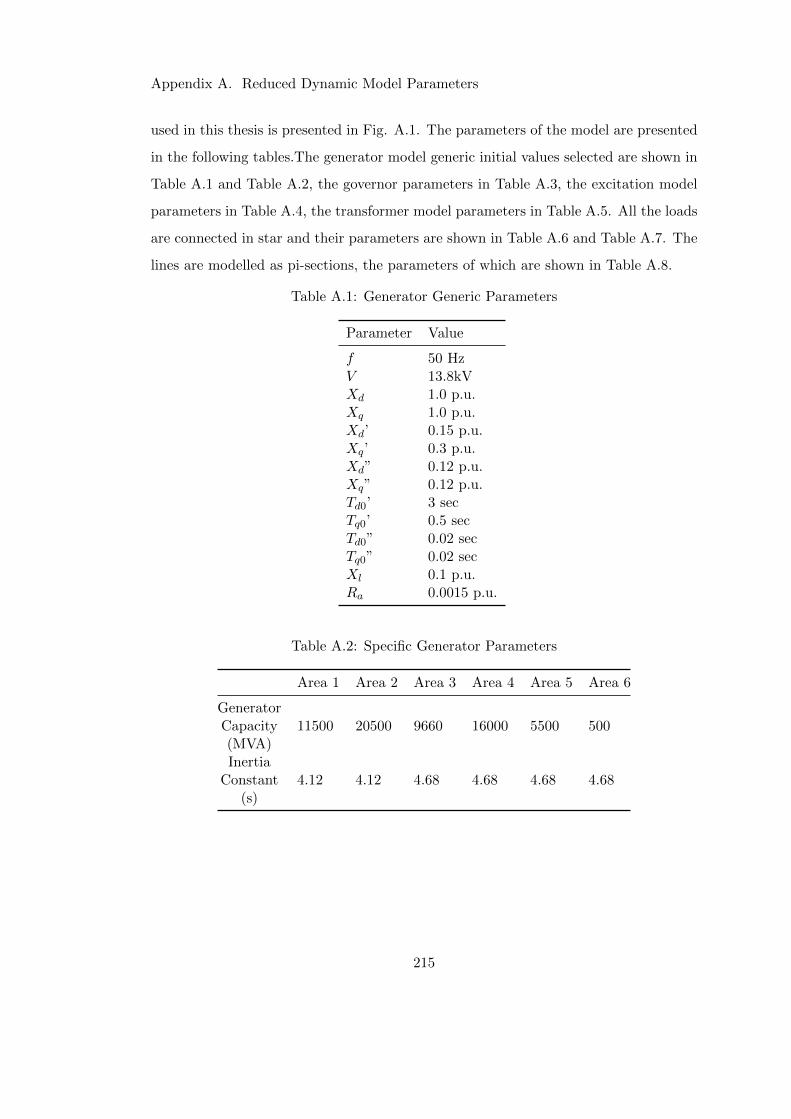
Appendix A. Reduced Dynamic Model Parameters
used in this thesis is presented in Fig. A.1. The parameters of the model are presented
in the following tables.The generator model generic initial values selected are shown in
Table A.1 and Table A.2, the governor parameters in Table A.3, the excitation model
parameters in Table A.4, the transformer model parameters in Table A.5. All the loads
are connected in star and their parameters are shown in Table A.6 and Table A.7. The
lines are modelled as pi-sections, the parameters of which are shown in Table A.8.
Table A.1: Generator Generic Parameters
Parameter Value
f 50 HzV 13.8kVXd 1.0 p.u.Xq 1.0 p.u.Xd’ 0.15 p.u.Xq’ 0.3 p.u.Xd” 0.12 p.u.Xq” 0.12 p.u.Td0’ 3 secTq0’ 0.5 secTd0” 0.02 secTq0” 0.02 secXl 0.1 p.u.Ra 0.0015 p.u.
Table A.2: Specific Generator Parameters
Area 1 Area 2 Area 3 Area 4 Area 5 Area 6
GeneratorCapacity(MVA)
11500 20500 9660 16000 5500 500
InertiaConstant
(s)4.12 4.12 4.68 4.68 4.68 4.68
215
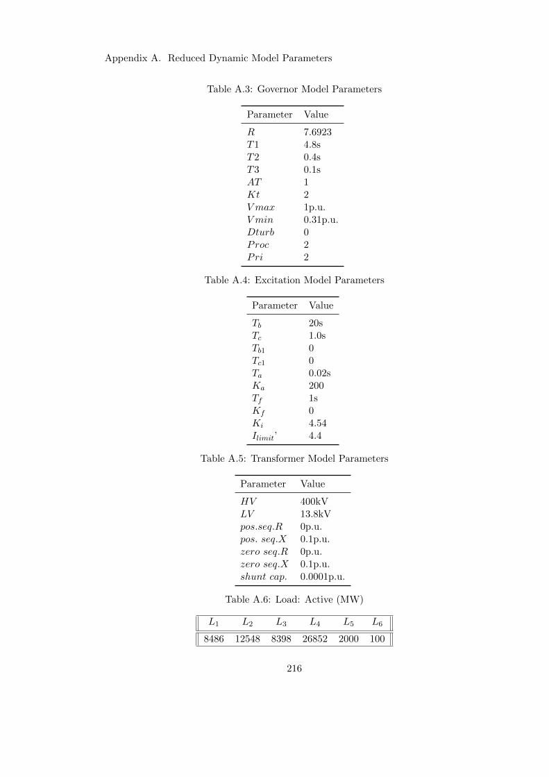
Appendix A. Reduced Dynamic Model Parameters
Table A.3: Governor Model Parameters
Parameter Value
R 7.6923T1 4.8sT2 0.4sT3 0.1sAT 1Kt 2V max 1p.u.V min 0.31p.u.Dturb 0Proc 2Pri 2
Table A.4: Excitation Model Parameters
Parameter Value
Tb 20sTc 1.0sTb1 0Tc1 0Ta 0.02sKa 200Tf 1sKf 0Ki 4.54Ilimit’ 4.4
Table A.5: Transformer Model Parameters
Parameter Value
HV 400kVLV 13.8kVpos.seq.R 0p.u.pos. seq.X 0.1p.u.zero seq.R 0p.u.zero seq.X 0.1p.u.shunt cap. 0.0001p.u.
Table A.6: Load: Active (MW)
L1 L2 L3 L4 L5 L6
8486 12548 8398 26852 2000 100
216
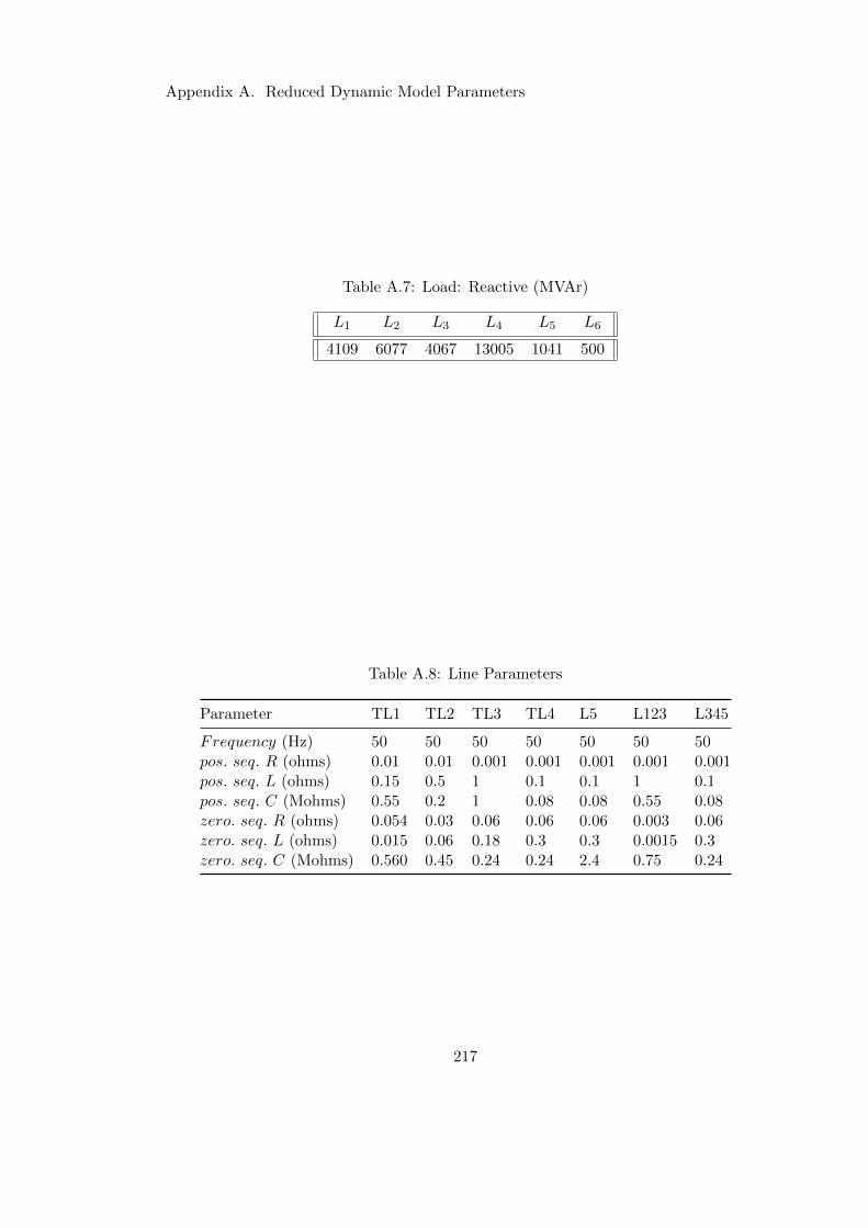
Appendix A. Reduced Dynamic Model Parameters
Table A.7: Load: Reactive (MVAr)
L1 L2 L3 L4 L5 L6
4109 6077 4067 13005 1041 500
Table A.8: Line Parameters
Parameter TL1 TL2 TL3 TL4 L5 L123 L345
Frequency (Hz) 50 50 50 50 50 50 50pos. seq. R (ohms) 0.01 0.01 0.001 0.001 0.001 0.001 0.001pos. seq. L (ohms) 0.15 0.5 1 0.1 0.1 1 0.1pos. seq. C (Mohms) 0.55 0.2 1 0.08 0.08 0.55 0.08zero. seq. R (ohms) 0.054 0.03 0.06 0.06 0.06 0.003 0.06zero. seq. L (ohms) 0.015 0.06 0.18 0.3 0.3 0.0015 0.3zero. seq. C (Mohms) 0.560 0.45 0.24 0.24 2.4 0.75 0.24
217