Embed Size (px)
Citation preview
Journal ofMARINE RESEARCHVolume 56 Number 1
Enhanced dispersion of near-inertial waves in an idealizedgeostrophic ow
by N J Balmforth1 Stefan G Llewellyn Smith1 and W R Young1
ABSTRACTThis paper presents a simpli ed model of the process through which a geostrophic ow enhances
the vertical propagation of near-inertial activity from the mixed layer into the deeper ocean Thegeostrophic ow is idealized as steady and barotropic with a sinusoidal dependence on thenorth-south coordinate the corresponding streamfunction takes the form c 5 2 C cos (2 a y)Near-inertial oscillations are considered in linear theory and disturbances are decomposed intohorizontal and vertical normal modes For this particular ow the horizontal modes are given interms of Mathieu functionsThe initial-value problem can then be solved by projecting onto this setof normal modes A detailed solution is presented for the case in which the mixed layer is set intomotion as a slab There is no initial horizontal structure in the model mixed layer rather horizontalstructure such as enhanced near-inertial energy in regions of negative vorticity is impressed on thenear-inertial elds by the pre-existinggeostrophic ow
Many details of the solution such as the rate at which near-inertial activity in the mixed layerdecays are controlled by the nondimensional number Y 5 4 C f0H mix
2 N mix2 where f0 is the inertial
frequencyHmix is the mixed-layer depth and Nmix is the buoyancy frequency immediately below thebase of the mixed layer When Y is large near-inertial activity in the mixed layer decays on atime-scale HmixNmix a 2 C 32f 0
12 When Y is small near-inertialactivity in the mixed layer decays on atime-scale proportional to N mix
2 H mix2 a 2C 2f0
1 Introduction
The vertical propagation of near-inertial oscillations (NIOs) from the mixed layer intothe thermocline is a crucial ingredient in current conceptions of how the upper ocean ismixed Local violations of the Miles-Howard stability criterion (eg Polzin 1996) are
1 Scripps Institution of Oceanography University of California at San Diego La Jolla California 92093-0230 USA
Journal of Marine Research 56 1ndash40 1998
1
thought to be created by the arrival of internal waves that are originally generated at eitherthe top or the bottom of the ocean As far as surface generation by wind events isconcerned one difficulty with this scenario is the very slow propagation rate of NIOs withlength scales characteristic of the atmospheric forcing mechanism Gill (1984) estimatedthat an NIO with a horizontal length scale of 1000 km will remain in the mixed layer forlonger than one year On the other hand observations do show that after a storm thenear-inertial energy in the mixed layer returns to background levels on a time scale of ten totwenty days (eg DrsquoAsaro et al 1995 van Meurs 1998) The implication is that at leastpart of this decay is associated with vertical transmission of near-inertial excitation into theupper ocean
DrsquoAsaro (1989) suggested a partial resolution of this problem he showed that theb -effect results in a steady increase of the north-south wavenumber of the NIO with timel(t ) 5 l(0) 2 b t Because the vertical group velocity of near-inertial waves is cg lt2 N 2(k2 1 l 2)2f0m3 the steady increase in l accelerates vertical propagationHowever thislsquo b -dispersionrsquo is only effective for the low vertical wavenumbers (notice that cg ~ m 2 3)which typically contain about 20 to 50 of the initial energy see Zervakis and Levine(1995) But b -dispersion cannot explain the vertical propagation of the remaining energynor the transmission of the near-inertial shear both of which are contained in the higherorder modes
The mechanism which is the focus of this paper is the refraction of NIOs by mesoscaleeddies Ray tracing studies have shown that geostrophic vorticity has an importantrefractive effect on near-inertial activity (Kunze 1985) Consequently several authorshave suggested that the mesoscale eddy eld plays a role in spatially modulatingnear-inertial activity (Weller et al 1991) and that enhanced vertical transmission isassociated with this induced spatial structure Indications of such an effect can be seen innumerical solutions such as those of Klein and Treguier (1995) DrsquoAsaro (1995a) vanMeurs (1998) and Lee and Niiler (1998)
Additional evidence that the mesoscale eddy eld accelerates the downward propagationof near-inertial oscillations comes from a recent theory by Young and Ben Jelloul (1997)This calculation involves an asymptotic reduction of the problem that lters the fast inertialoscillations and isolates the slower subinertial evolution of the amplitude Young and BenJelloul employ the resulting reduced equations to show that the recti ed effect of small-(relative to the initial scale of the NIO) scale geostrophic eddies can induce verticaldispersion of near-inertial waves In this paper we continue in the vein proposed by Youngand Ben Jelloul We use their reduced description to study vertical dispersion induced bymesoscale motions One important advantage of this approach over ray-tracing is that it isnot necessary to assume that the scale of the near-inertial waves is much less than that ofthe mesoscale eddies Indeed in the ocean near-inertial waves are forced on the largespatial scales characteristic of atmospheric storm systems so that the WKB approximationis not applicable
Our larger purpose in this work is to lay the wave-mechanical foundation for a theory of
2 Journal of Marine Research [56 1
NIO propagation through the strongly inhomogeneous environment of the mesoscale eddy eld But we must start with a simple theoretical formulation rather than with complicatedmodels of geostrophic turbulence In this paper in fact we attempt only to construct thesimplest model we can think of which has some expectation of representing the realphysical situation of very large-scale near-inertial excitation superposed on a smaller scalegeostrophic ow
The simpli ed model is similar to the initial value problem of Gill (1984) at t 5 0 themixed layer moves as a slab and the deeper water is motionless Gill consideredbackground states without barotropic ow and modulated the initial slab velocity with ahorizontal structure proportional to cos ly In Gillrsquos problem the lengthscale l 2 1 is vital insetting the rate at which the near-inertial activity in the mixed layer decays if l 5 0 then themixed layer oscillates unendingly at precisely the inertial frequency there is no verticaltransmission and no decay of the inertial oscillations in the mixed layer We depart fromGillrsquos analysis by introducing a background geostrophic ow We show that even if initialconditions are horizontally homogeneous (l 5 0) the pre-existing geostrophic ow im-presses horizontal structure on the near-inertial motion and a relatively rapid verticaltransmission ensues We idealize this lsquobackgroundrsquo as a steady barotropic unidirectionalvelocity with sinusoidal variation c 5 2 C cos 2 a y
We use a single sinusoid c ~ cos (2 a y) as a background ow because the model isintended to represent the propagation of NIOs in a simple environment such as the site ofthe Ocean Storms experiment in the Northeast Paci c (see DrsquoAsaro et al 1995) We arenot concerned with near-inertial propagation through spatially localized features such asintense jet (for example Rubenstein and Roberts 1986 Wang 1991 Klein and Treguier1995) or Gulf Stream Rings (Kunze et al 1995 Lee and Niiler 1998)
Our goal is to answer several basic questions within the context of the simple modeloutlined above These questions are
(i) How rapidly do the inertial oscillations in the mixed layer decay and what featuresof the background determine the timescale of this decay
(ii) Does the near-inertial activity in the mixed layer develop strong spatial modula-tions during the decay process
(iii) Does the dispersal of near-inertial waves into the upper ocean result in theformation of isolated maxima in energy below the mixed layer
The rst question is directed at the issue of the decay of near-inertial energy and shear inthe mixed layer given that b -dispersion is ineffective for the high vertical modes can therefractive effects of a geostrophic ow result in enhanced vertical propagation of smallvertical scales The second and third questions are motivated by observations made duringthe Ocean Storms experiment First using drifter data van Meurs (1998) observed thatdepending on spatial location near-inertial oscillations in the mixed layer disappear ontimescales which vary between 2 days and 20 days Second the mooring data summarized
1998] 3Balmforth et al Dispersion of near-inertial waves
by DrsquoAsaro et al (1995) showed that as the inertial energy in the mixed layer decreases astrong maximum in inertial energy appears at around 100 m (this was called a lsquobeamrsquo)
Our solution method is an expansion in the normal modes (both horizontal and vertical)of the problem the details of these modes and how we superpose them to solve the initialvalue problem are given in Sections 2 through 4 Section 5 deals with visualizing theresults In Section 6 we discuss some limiting cases in which analytical approximationsprovide insight We sum up in Section 7
2 Formulation for a barotropic and unidirectional geostrophic ow
Our point of departure is the NIO equation of Young and Ben Jelloul To leading orderthe NIO velocity eld (u v w) buoyancy b and pressure p are expressed in terms of acomplex eld A (x y z t)
u 1 iv 5 e 2 if0tL A
w 5 21
2f 0
2N 2 2( Azx 2 i Ayz )e 2 if0t 1 cc
b 5i
2f0 ( Azx 2 i Ayz )e 2 if0t 1 cc
p 5i
2f0 ( Ax 2 i Ay)e 2 if0t 1 cc
(21andashd)
where L is a differential operator de ned by
L A ( f 02N 2 1 Az )z (22)
and N(z) is the buoyancy frequency Thus the complex function A concisely describes allof the NIO elds
If the background geostrophic ow is barotropic when A evolves according to theequation
L At 1shy ( c L A )
shy (x y)1
i
2f0 = 2 A 1 i 1 b y 1
1
2z 2 L A 5 0 (23)
In (23) c (x y) is the steady barotropic streamfunction and z = 2c is the correspondingvorticity Throughout this paper = 2 is the horizontal Laplacian ie = 2 5 shy x
2 1 shy y2 The
boundary condition is that Az 5 0 at the top and bottom of the ocean from (21b) thisensures that w vanishes on the boundaries
The approximate description in (23) is obtained by applying a multiple timescaleapproximation to the linearized primitive equations the linearization is around thegeostrophic background ow c The small parameter in the expansion is essentially( v 2 f0)f0 that is the departure of the wave frequency from the inertial frequency Thereis no assumption of spatial scale separation between the geostrophic background ow and
4 Journal of Marine Research [56 1
the near-inertial wave The evolution equation in (23) displays the processes whichdetermine the subinertial evolution of the near-inertial part of the wave spectrum namelyadvection dispersion and refraction by the combination b y 1 ( z 2)
In Gillrsquos (1984) notation the Sturm-Liouville problem associated with the linearoperator L is
Lpn 1 f 02c n
2 2pn 5 0 (24)
where the eigenvalue cn 5 f0Rn is the speed of mode n and Rn is the Rossby radius Withthe barotropic idealization c z 5 0 one can project A onto the basis set in (24)
A (x y z t) 5 Sn5 1
`
An(x y t)pn (z) (25)
Each modal amplitude then satis es the Schrodinger-like equation
shy An
shy t1
shy ( c An )
shy (x y)1 i 1 b y 1
1
2z 2 An 5
i n
2= 2 An (26)
where
n f0Rn2 (27)
is the lsquodispersivityrsquoof mode n We will solve (26) as an initial value problem in Section 4To make an analogy with quantum mechanics rewrite Eq (26) as
i n
shy An
shy t5
1
2(i n = 2 u)2 An 1 Vn An (28)
where
Vn n3 b y 11
2z 4 2
1
2u middot u
(29ab)u 5 z 3 = c
After notational changes Eq (28) is the same as Schrodingerrsquos equation for the motion ofa particle (with mass m 5 1) in a magnetic eld = 2 c z In this analogy the geostrophicvelocityu 5 z 3 = c is the vector potential of the magnetic eld (usually denoted by A inquantum mechanics) and Vn is the potential function The quantum analogy is awedbecause the potential Vn contains the term u middot u2 and there is no equivalent term in thequantum mechanical case Nonetheless the quantum analogy is suggestive and useful2
2 For instance if c 5 0 then (28) is equivalent to the motion of a particle falling in a uniform gravitationalpotential n b y Thus particles (ie near-inertial wave packets) accelerate toward the equator with gn 5 b nDrsquoAsarorsquos (1989) result that l(t) 5 l(0) 2 b t is the linear-in-time momentum increase occurring as a particle fallsin a uniform gravitational eld The paths of wave packet centers in the (x y)-plane are the parabolic trajectoriesof ballistically launched particles
1998] 5Balmforth et al Dispersion of near-inertial waves
We now limit attention to zonal parallel ows that is c x 5 0 and z 5 c yy One can thensolve (26) by looking for normal mode solutions with
An (x y t ) 5 An(y) exp (ikx 2 iv nt) (210)
The resulting eigenproblem for v n is
n
d2An
dy21 [2 v n 2 nk 2 2 F ]An 5 0 (211)
where
F (y) 5 c yy 2 2kc y 1 2 b y (212)
In the remainder of this paper we construct the solutions of the eigenproblem in (211)then solve the initial value problem
Earlier studies of NIO interaction with geostrophic ows have emphasized that wavesare concentrated in regions of negative z 5 c yy (Kunze 1985 Rubenstein and Roberts1986 Klein and Treguier 1995) On the other hand the quantum analogy suggests that thesolution of (211) will be large in regions where F is negative (ie inside potential wells)Provided that F lt c yy there is agreement between these two approaches
3 The normal modes for a sinusoidal shear ow
We now consider the sinusoidal barotropic ow with associated streamfunction
c 5 2 C cos (2 a y) (31)
where for de niteness we take C 0 We also take b 5 0 The potential function F ( y) in(212) can then be put in the form
F 5 4 a Icirc a 2 1 k 2 C cos 2 h h a y 1g
2 (32ab)
where
sin g 5 k Y Icirc a 2 1 k 2 cos g 5 a Y Icirc a 2 1 k 2 (32cd)
Hence (211) can be written as
d2An
d h 21 (a 2 2q cos 2h )An 5 0 (33a)
where
a (2 v 2 nk2 ) Y n a 2 q 2 C Icirc 1 1 a 2 2k2 Y n (33bc)
The differential equation (33a) is Mathieursquos equation (Abramowitz and Stegun 1972)
6 Journal of Marine Research [56 1
From this point forward we take k 5 0 It is clear from (32) and (33) that nonzero k hasno qualitative effects provided that k a frac12 1 for NIOs forced by large-scale winds this isthe case In the special case k 5 0 the Mathieu equation can also be derived directly fromthe primitive equationsmdashsee AppendixA
a Solutions of Mathieursquos equation
Mathieu functions are examples of classical special functions and descriptions of themmay be found in texts (eg Abramowitz and Stegun 1972 Brillouin 1946 McLachlan1947) However these particular special functions are neither common nor are theymembers of the hypergeometric family and so we give a rudimentary discussion of them
It follows from Floquet theory that every solution of Mathieursquos equation (32) can beexpressed in the form
An( h ) 5 e i n h P( h a q) (34)
where n (a q) (the lsquolsquocharacteristic exponentrsquorsquo or Bloch wavenumber in quantum mechan-ics) is a (possibly complex) function of a and q and P( h a q) is a periodic function ofperiod p There is a special class of solutions in which n (a q) 5 0 so that A in (34) is aperiodic function of h These periodic functions are the lsquoMathieu functions of integerorderrsquo because n 5 0 these functions exist only on a set of curves in the (a q) parameterplane These curves displayed in Figure 201 of Abramowitz and Stegun (1972) de ne theeigenvalue a as a function of the parameter q
The Mathieu functions of integer order r divide into even solutions cer( h q) and intoodd ones ser( h q) the integer index r 5 0 1 is the horizontal mode number Thesesolutions have the eigenvalues ar(q) and br(q) respectively Linear combinations ofMathieu functions of integer order can be used to represent any function which has theperiodicity F( h ) 5 F( h 1 p ) this completeness is the basis of our solution in Section 4More precisely we will be concerned with solving the NIO equation subject to an initialcondition which is uniform in the horizontal That is we are interested in a situation inwhich we need to express a constant initial condition in terms of the normal modesolutions Since a constant is a (trivial) example of a function with period p the particularsolutions of (32) which we need are precisely the Mathieu functions of integer orderMoreover since only even modes project onto that constant we need only the Mathieufunctions of even integer order denoted by cer( h q) Hence from this point forward wefocus entirely on these speci c solutions these modes are the building blocks used inSection 4 (We would need a more general class of modal solutions including both the oddMathieu functions ser( h q) and the other nonperiodic solutions with n THORN 0 were we toconsider an initial condition with more complicated horizontal structure)
1998] 7Balmforth et al Dispersion of near-inertial waves
b The Mathieu functions of even integer order
We use the package written by Shirts (1993) and available from httpgamsnistgov tocompute the Mathieu functions of integer order In Figures 1 and 2 we display the structureof the lower order even Mathieu functions In Figure 1a we show the functions ce0( h q)for various values of q Notice that ce0( h 0) 5 1 Icirc 2 but as q increases the eigenmodece0( h q) becomes increasingly concentrated to the vicinity of h 5 p 2 This correspondsto a localization of the mode to the region where the geostrophic vorticity 4a 2C cos (2 h )is negative (the minima of the quantum mechanical potential)
Figure 1b shows the same transition for the eigenfunction ce4( h q) The localization isillustrated further in Figure 2 which shows cer( h 100) with r 5 0 1 and 2 the main pointto note here is the general trend that the higher-order eigenmodes are less concentrated thanthe low-order modes
The most physically relevant quantity is the eigenfrequency v rn In order to determinethese modal frequencies we need to rst specify q then obtain the appropriate eigenvaluear(q) from (32) Finally using (33b)
v rn 51
2a 2 nar(2 C n ) (35)
A more revealing way of representing the dispersion relation (35) is to observe fromL An 1 R n
2 2 An 5 0 that the Rossby radius of deformation of the nth vertical mode Rnand the local vertical wavenumber m(z) are related by
m (z) 5 N (z)f0Rn (36)
On combining the above with (27) and (33c) we obtain
q 52 C f0
N 2m 2 (37)
The expression in (37) motivates the de nition of a dimensionless vertical wavenumber as
m Icirc 2 C f0
N 2m (38a)
or equivalently m 5 Icirc q Now de ne a dimensionless frequency as
v ˆ 2v z min (38b)
where z min 2 4 a 2 C 0 is the most negative value of the geostrophic vorticity Thesede nitions put (35) into the compact form
v ˆ 51
2m 2ar (m 2 ) (39)
8 Journal of Marine Research [56 1
Figure 1 (a) Mathieu functions ce0( h q) with q 5 0 through 5 then q 5 10 followed by steps of 10until q 5 100 (b) Mathieu functions ce4(h q) at the same values of q as part (a) Notice thatce0( h 0) 5 1 Icirc 2 and ce4(h 0) 5 cos (4h ) As q increases both of these eigenfunctions becomeconcentrated around the vorticity minimum at h 5 p 2
1998] 9Balmforth et al Dispersion of near-inertial waves
where the index r 5 0 1 middot middot middot is the horizontal mode number In Figure 3 we show thedispersion relation of the even modes with r 5 0 2 middot middot middot 20 All of the eigenbranchesslowly asymptote to v ˆ 5 2 1 corresponding to a dimensional frequency shift of z min2 (cfKunze 1985)
We summarize our progress by saying that there is a set of two-dimensional eigenfunc-tions pn (z)cer ( a y 2C f0Rn
2 ) The eigenfunctions are indexed by (n r) and the eigenfre-quencies are given by (35)
c Representation of one as a sum of Mathieu eigenfunctions
In the next section we solve (26) as an initial value problem with An( y t 5 0) 5 1This is accomplished by projecting the initial condition onto the eigenmodes describedabove that is by representing 1 as a sum of Mathieu functionsThe orthogonalityproperty
e 0
2pce n ( h q)cemicro (h q) dh 5 p d micron (310)
can be used to deduce the representation
1 51
p Sr 8 5 0
`
J 2r 8(q)ce2r 8( h q) (311a)
Figure 2 The three Mathieu functions ce0(h 100) ce1(h 100) and ce2( h 100) As the index rincreases the function becomes less localized Notice also that ce1 is antisymmetric around h 5p 2 This antisymmetry ensures that ce1 does not project onto 1 in the sum (311a)
10 Journal of Marine Research [56 1
where
J r (q) e 0
2 pcer ( h q) d h (311b)
In the notation of Abramowitz and Stegun (1972) J r(q) 5 A 0r (q) due to our alternative
use of lsquoArsquo we prefer to introduce the quantity in (311b) Because of symmetry the oddeigenfunctions ser( h q) do not appear in the series (311a) There is also a furthersymmetry evident in the graph of ce1 in Figure 2 that removes the functions ce2r8 1 1( h q)from the series (ie J 2r8 1 1(q) 5 0)
The series in (311a) converges very quickly in fact if q 5 0 one term is exact If q frac34 1the convergence is still very fast Figure 4 shows the partial sums of (311a) with q 5 100Using eleven terms (this is the truncation we employ in Section 5) the error is less than onepercent
4 The initial value problem
In this section we solve the initial value problem by projection onto the modes describedabove Up to this point we have avoided making a particular choice of buoyancy pro leN(z) But now we need to specify the vertical modes and so we adopt Gillrsquos (1984) modelbuoyancy pro le which combines analytical simplicity with physical realism Zervakis and
Figure 3 The dimensionless frequency v ˆ in (38b) as a function of the dimensionlesswavenumberm 5 Icirc q We show only the dispersion relations of the eigenfunctions ce2r8( h q) which appear in(311a) (r8 5 0 through r8 5 10)All of the curves asymptote to v ˆ 5 2 1 In anticipationof resultsfrom Section 6 we show the strong dispersion approximation as the dashed curve v ˆ 5 2 m24labelled lsquoSDArsquo Notice that the strong dispersionapproximationcaptures only the r 5 0 branch
1998] 11Balmforth et al Dispersion of near-inertial waves
Levine (1995) provide some useful additional information concerning the properties ofthese vertical modes
a Gillrsquos buoyancy pro le
Gillrsquos buoyancy pro le is
N (z) 5 50 if 2 Hmix z 0
s(z0 2 H 2 z) if 2 H z 2 Hmix(41)
(Gill placed z 5 0 at the bottom of the ocean we prefer to use the convention that z 5 0 isthe surface of the ocean) Typical values for the parameters are given in Table 1 Asmentioned in Section 2 there is a set of Sturm-Liouville eigenfunctions that satisfy
dpn
dz5 2 N 2hn cn
2dhn
dz5 pn (42ab)
where cn 5 f0Rn is the eigenspeed Gillrsquos analytic solution for hn and pn arises on solving(42ab) with (41)
Figure 5 summarizes the solution of the eigenproblem by showing qn2 5 2 C f0n 2R n2 as
a function of n Figure 5 can be used to quickly estimate the value of q which is used in thesolution of the horizontal eigenproblem (33a) For instance suppose that one is interested
Figure 4 The series in (311a) truncated after the indicated number of terms Because (311a) isrepresenting a smooth periodic function (viz one) as a superposition of smooth periodicfunctions (viz cer( h 100)) there is no Gibbsrsquo phenomenon and the error of the truncated sumeventually decays exponentiallyas the number of retained terms increases
12 Journal of Marine Research [56 1
Table 1 Numerical values of the parameters used in the calculationsThe numerical values of C a Y and T refer to the lsquostandard casersquo of Section 5b
Quantity Symbol Typical numerical value
Ocean depth H 4200 mMixed layer depth Hmix 50 mStrati cation parameter s 25 m s2 1
Vertical scale of N z0 43296 mN at base of mixed layer Nmix 001392 s 2 1
Inertial frequency f0 10 2 4 s 2 1
Length scale of geostrophic ow a 2 1 80000 mMaximum geostrophic streamfunction C 4000 m2 s 2 1
Minimum geostrophic vorticity z min 5 2 4 a 2C 2 25 3 10 2 6 s 2 1
Kinetic energy density K 5 (a C )2 1400 m2 s2 2
Time scale T 5 2 z min 926 daysNondimensionalocean depth H 83Nondimensional strati cation parameter micro 0139Nondimensionalgeostrophic ow strength Y 3302Normalization constant N 1200
Figure 5 A plot of 2 C n 2R n2 f0 versus vertical mode number n The modal speed cn 5 f0Rn is the
eigenvalue obtained from solving the vertical eigenproblem in (41) and (42) We use thenumerical values from Table 1 ie C 5 4000 m2 s2 1 Using the combination qn2 on the verticalaxis removes the strongest dependence on the vertical mode number
1998] 13Balmforth et al Dispersion of near-inertial waves
in vertical mode number n 5 10 and C 5 4000 m2 s 2 1 Then it follows from Figure 5 thatq(10)2 5 0115 or q 5 115 Using Figures 1 and 2 one can then get some impression ofthe structure of the horizontal modes with the common vertical mode number n 5 10
The eigenmodes in (42a) are orthogonal
e 0
Hpn (z)pm(z) dz 5 (Hmixs n )d mn e 0
HN 2 (z)hn(z)hm(z) dz 5 (Hmixcn
2 s n ) d mn (43ab)
where the normalization constant s n is de ned in Eq (A9) of Gill3
b The vertical structure of the initial condition
Gill considered an initial condition in which the mixed layer moves as a slab Here weuse a modi ed form of Gillrsquos initial condition Speci cally we take
uI(z) Sn 5 1
80
e ns npn (z) e n N exp ( 2 n 2600) (44ab)
and vI(z) 5 0 The normalization factor N in (43b) is computed to ensure that uI(0) 5 1The initial condition (43) is shown in Figure 6 As a result of truncating the sum at n 5 80and including the low pass lter e n there is now some initial excitation in about the rst 20
3 There is a misprint in (A9) of Gill With the notation of that Appendix the expression for s n should be
s n 5 2 e 1 1 1e
22 m 2 5 1 m 2 11
42 [ e 1 j T (1 1 e 2m 2 )] 62 1
Figure 6 The initial velocity uI(z) and the initial shear duI(z)dz (solid and dashed respectively)calculated from (44) The highest vertical eigenmode n 5 80 is shown in the left-hand portion ofthe gure The function p80(z) is shown by the solid curve and h80(z) by the dotted curve
14 Journal of Marine Research [56 1
meters below the mixed layer This is probably more realistic than a completely discontinu-ous initial condition Further since we are interested in examining the evolution of thevertical shear we must have an initial condition in which the shear is nite the initial shearpro le in Figure 6 is consistent with the observation of shear concentration at the base ofthe mixed layer
Additional motivation for the initial condition in Figure 6 is provided by the very slowconvergence of the un ltered series to Gillrsquos discontinuous initial velocity For instance ifthe un ltered series is truncated after P terms then the error is O(1P) Further the initialcondition de ned by a truncated sum exhibits Gibbsrsquo phenomenon even with P 5 120terms there is unrealistic oscillatory structure at relatively deep levels The ltering factore n eliminates this lsquolsquoringingrsquoand provides a strongly localized initial excitation
c Projection of the initial condition on the modes
We now represent A ( y z t ) as a sum of vertical normal modes as in (25) and projectthe initial condition L A ( y z 0) 5 uI(z) in (44) onto this basis set The result is that
An (y 0) 5 2 R n2e ns n (45)
Thus after the projection on vertical normal modes the problem is to solve
shy An
shy t1 2ia 2C cos (2a y) An 5
i
2 n
shy 2 An
shy y2 (46)
with the initial condition in (45)Next we use (311a) to project the initial condition (45) onto horizontal eigenmodes
This gives
An (y t ) 5 2 R n2e ns n S
r 8 5 0
`
J 2r8n exp ( 2 iv 2r8nt ) ce2r 8 (a y 2 C n ) (47)
where J 2r8n J 2r8(2 C n) The frequency of the mode with index (2r8 n) is as beforev 2r8n 5 na 2a2r8(2 C n)2
d Reconstruction of the velocity and the shear
To reconstruct the nal elds one must sum (47) over the vertical mode number nThus using (21a) with Lpn 5 2 Rn
2 2pn one nds that the horizontal velocities are given by
u 1 iv 5 e 2 if0t Sn5 1
80
Sr 8 5 0
10
e n s n J 2r 8n exp ( 2 i v 2r 8nt ) ce2r 8( a y 2C n) pn (z) (48)
The sum over r8 in (48) has been truncated after eleven terms this is more than enough toensure convergence (see Fig 4) In addition one obtains from (48) the following
1998] 15Balmforth et al Dispersion of near-inertial waves
expression for the vertical shear
uz1 ivz 5 2 e 2 if0tN 2 Sn5 1
80
Sr 8 5 0
10
e n s n J 2r 8n exp ( 2 iv 2r 8nt ) ce2r 8( a y 2 C n ) hn(z) (49)
where hn is de ned in (42) The series in (48) and (49) are our solution of the initial valueproblem posed in Figure 6
Before attemptingvisualizationof the solution let us examine the spectral decay of (48)and (49) Using the orthogonality relations in (43) the total squared velocity is
e 0
2p a
e 0
H(u 2 1 v2 ) dz dy 5 p Hmix a
2 1 Sn 5 1
80
Sr 8 5 0
10
e n2s nJ 2r 8n
2 (410)
from which we can read off the fraction of energy contained in the mode (r8 n)
E2r 8n e n2s nJ 2r 8n
2 Y Sn5 1
80
Sr 8 5 0
10
e n2 s n J 2r 8n
2 (411)
This modal energy fraction is shown in Figure 7aThe modal content of the total squared shear is a little more difficult to estimate because
the functions N 2 n(z) are not orthogonal Hence the total square shear
e 0
2p a
e 0
H(u z
2 1 v z2 ) dz dy (412)
does not separate into a convenient sum over squares of modal amplitudes However theorthogonality relation (43b) shows that the functions Nhn(z) are orthogonal Hence weestimate the modal content of the mean square shear using the weighted average
e 0
2p a
e 0
HN 2 2 (u z
2 1 v z2 ) dz dy (413)
Thence the fraction of the weighted mean square shear in the mode (r8 n) is given by
S2r8n e n2s nJ 2r 8n
2 c n2 2 Y Sn 5 1
80
Sr 8 5 0
10
laquo n2 s n J 2r 8n
2 c n2 2 (414)
which is shown in Figure 7b Notice that the expression in (413) is proportional to anlsquoinverse Richardson numberrsquo averaged over the volume of the uid Thus S2r8n in (414) isthe contributionof mode (2r8 n) to the inverse Richardson number
Figure 7 shows that the truncation in (48) is sufficient to resolve both the velocity andshear The velocity is heavily concentrated in the low modes In particular the modes withhorizontal mode number r 5 0 contain over 85 of the energy On the other hand the shearis distributed more evenly over higher modes (note the different scales of the vertical axesin the two parts of Fig 7)
16 Journal of Marine Research [56 1
Another view of the initial excitation is shown in Figure 8 where E2r8n is plotted againstthe dimensionless modal eigenfrequency v ˆ in (39) It is signi cant that the eigenfrequen-cies with v ˆ lt 2 1 (that is dimensional frequencies close to z min2) do not contain muchenergy This might bear on DrsquoAsarorsquos (1995b) unsuccessful attempt to observe a z 2frequency shift using the Ocean Storms data set Our model initial condition simply doesnot excite modes with eigenfrequencies close to z min2 In fact the concept of a spatiallylocal frequency shift is usually meaningless when one has eigenmodes The conceptacquires some meaning if the eigenmodes are spatially localized near a potentialminimum
Figure 7 (a) Upper panel the fraction of energy E2r8n in (411) in the mode (2r8 n) Notice that theaxis is r 5 2r8 Most of the energy is contained in the rst two horizontal modes with r8 5 0 andr8 5 1 (b) Lower panel the fraction of square shear (or inverse Richardson number) S2r8n in(414) in mode (2r8 n) Note the different scales on the vertical axes in (a) and (b) As expectedhigher modes make a more important contribution to the shear
1998] 17Balmforth et al Dispersion of near-inertial waves
this is why the eigencurves in Figure 3 asymptote to v ˆ 5 2 1 (corresponding to z min2) Butto strongly excite such localized modes we would need a very different initial condition
5 Results
a Dimensional considerations
To systematically discuss the results of parametric variations we must rst consider thenondimensional form of the problem As nondimensional independent variables we use
t tT h a y z 5 (z 1 Hmix)Hmix (51)
where following our earlier de nition of the nondimensional frequency in (38b) thetimescale is T 5 2 z min For the sinusoidal ow in (31) this choice of T is equivalent to
T 1
2 a 2 C (52)
The nondimensional vertical coordinate is 2 H z 1 where the nondimensional oceandepth is H (H 2 Hmix)Hmix Notice that z 5 0 is the base of the mixed layer and z 5 1 isthe ocean surface The buoyancy frequency can be measured in units of its value directly
Figure 8 The fraction of energy in mode (2r8 n) E2r8n in (411) plotted against the nondimensionalmodal frequency 2 v 2r8nz min The horizontal axis is truncated at v ˆ 5 25 there are higherfrequencies in the series (48)
18 Journal of Marine Research [56 1
beneath the mixed layer Nmix for the particular pro le of (41) we then nd
N (z) 5 50 if 0 z 1
1(1 2 2microz) if 2 H z 0(53)
where micro Hmix2(z0 1 Hmix 2 H ) and Nmix s(z0 2 H 1 Hmix)The nondimensional form of the A equation can then be written
Y [L A t 1 i cos 2 h L A ] 1 i A h h 5 0 (54)
where L is the nondimensional differential operator
L 5 shy z N 2 2 shy z (55)
The most important nondimensionalparameter in the problem is
Y 4C f0
Hmix2 Nmix
2 (56)
Y is a measure of the strength of the geostrophic ow speci cally Y z minV where V a 2Hmix
2 Nmix2 f0 is the back-rotated frequency of a wave whose horizontal scale is that of the
geostrophic ow and whose vertical scale is the mixed layer depthThe solution of the initial value problem is discussed mainly using dimensional
variables However the considerations above show that there are only three independentnondimensional parameters viz micro H and Y In fact of the parameters in the barotropicstreamfunction C and a the length scale a 2 1 appears only in the time scale T Hencechanges in the strength of background ow are made by modifying C which is equivalentto changing Y
b The standard case
We now examine the temporal behavior of the solution for a particular selection ofmodel parameters which we refer to as the lsquostandardrsquocase (we use the label S to signify thiscase in subsequent gures) these choices are listed in Table 1 Figures 9ndash11 summarize theresults because Y 5 3302 (corresponding to a peak velocity of 10 cm s 2 1) the standardcase has a fairly strong background ow
In Figure 9 we show how the lsquospeedrsquo Icirc L A L A 5 Icirc u2 1 v 2 evolves in timeInitially the speed is sharply concentrated in and just below the mixed layer (see Fig 6)But after 10 days (Fig 9a) the development of both horizontal and vertical structure isevident
In the mixed layer itself the sinusoidal barotropic ow (c z ) ~ cos 2h impresses ananalogous modulation cos 2h on the NIO speed In fact the modulation is so strong that itincreases the speed by about 20 over its initial value in the vicinity of the vorticityminima ( h 5 p 2) The structure is very different directly below the mixed layer Enhanced
1998] 19Balmforth et al Dispersion of near-inertial waves
downward propagation is correlated with both the maxima and the minima of the vorticitythis results in a second harmonic cos 4 h structure in the NIO speed below the mixed layer
In some respects these patterns agree with the observations described by van Meurs(1998) First the rate at which near-inertial activity lsquodisappearsrsquo from the mixed layer isspatially inhomogeneousvan Meurs observed that the time scale varied between 2 and 20
Figure 9 Panels (a)ndash(f) show snapshots of the speed L A ( y z t ) 5 Icirc u2 1 v 2 as surface plotsabove the ( h z) plane every 10 days after the initiation of the near-inertialoscillationThe depth zis in meters and h 5 2 a y is dimensionless
20 Journal of Marine Research [56 1
days depending on locationvan Meurs also attempted to correlate the energy level with thegeostrophic vorticity Figure 9a suggests that in the mixed layer there is a strongcorrelation high NIO energy with negative vorticity (eg h 5 p 2) and low NIO energywith positive vorticity (eg h 5 0 and p ) Such a correlation was not seen unambiguouslyin van Meursrsquos drifter observations It may be that the mesoscale vorticity is not wellresolved by this data set Alternatively if some of the drifters happened to be drogued to uid beneath the mixed layer then those drifters would see elevated energy levels at boththe maxima and minima of the vorticity (as in Fig 9a)
By 20 days the spatial pattern is even clearer (Fig 9b) Notice that near the vorticitymaxima ( h 5 0 and p ) the speed now has a submixed-layer maximum In other words itappears as though the near-inertial energy has been expelled from the mixed layer at h 5 0and p and concentrated just below the base of the mixed layer These concentrations ofactivity subsequently propagate horizontally (Figs 9bndash9e) and add to downwardly propa-gating oscillations from the mixed layer near h 5 p 2 This results in the formation of asubstantial peak in speed just below the mixed layer at the vorticity minima ( h 5 p 2)
Over this period the activity in the mixed layer near the vorticity minimum begins todecline Eventually in Figures 9dndashf the near-inertial activity disperses downward At thevorticity minimum ( h 5 p 2) the mixed-layer speed nally falls below its initial level By60 days activity remains peaked below the mixed layer at the vorticity minimum and verydeep penetrationof near-inertial activity takes place only in regions of positive vorticity (inFig 9f near h 5 0 and p the speed is fairly uniform over the top 1000 m)
More quantitative features of the solution are shown in Figures 10 and 11 Figure 10shows the backrotated velocity eld below both the maximum (Fig 10a) and the minimum(Fig 10b) of the vorticity The contours in Figure 10 are curves of constant speed Bothparts of Figure 10 show the formation of what DrsquoAsaro et al (1995) call a lsquolsquobeamrsquorsquo InFigure 10b the lsquolsquobeamrsquorsquo is composed of strong inertial currents below the mixed layer andis located roughly in the region between z 5 2 50 m and z 5 2 100 m In fact as thecontour labelled 125 indicates the speed can be larger than that of the initial conditionThe lsquolsquobeamrsquorsquo is also apparent though less intense in Figure 10a
Figure 11 shows the backrotated shear vectors below the maximum (Fig 11a) andminimum (Fig 11b) of the vorticity Because the shear eld is shallower and has moresmall-scale structure than the velocity eld we have changed the depth scale relative tothat of Figure 10 We have also not shown the mixed layer (where the shear is zero) Thereare interesting qualitative differences between Figure 11a and 11b (The differences aregreater than those between Figs 10a and 10b)
c Parametric variations
As gross indications of how changes in the parameters alter the evolution we use twoaveraged measures of the inertial activity in the mixed layer
1998] 21Balmforth et al Dispersion of near-inertial waves
Figure 10 Temporal evolution of the backrotatedvelocity eld (u v) with depth z (meters) at (a) thevorticity maxima (h 5 0 p ) and (b) the vorticity minima (h 5 p 2 3 p 2 ) Shown arethe backrotated velocity vectors at the points (t z) The contours are curves of constant speed
Icirc u 2 1 v2 The initial speed in the mixed layer is 1 and the contour interval is 02
22 Journal of Marine Research [56 1
Figure 11 Temporal evolution of the backrotated shear eld (uz vz) with depth z (meters) at (a) thevorticity maxima (h 5 0 p ) and (b) the vorticity minima (h 5 p 2 3 p 2 ) Note Thedepth scale in this gure differs from that of Figure 10 Shown are the backrotated shear vectors at
the points (t z) The contours are curves of constant shear strength Icirc u z2 1 v z
2 In the initialcondition the shear has a maximum value of 514
1998] 23Balmforth et al Dispersion of near-inertial waves
First from (311a) and (47) we obtain the horizontally averaged velocity
7 u 1 iv8 a
p e 0
p a(u 1 iv) dy
51
2 pe 2 i f0t S
n 5 1
80
Sr 8 5 0
10
e n s n exp ( 2 iv 2r 8nt ) J 2r 8n2 pn(z)
(57)
In the mixed layer the expression above simpli es because pn(z) 5 1 Thus one measureof inertial activity obtained from (57) with pn 5 1 is the magnitude of the horizontallyaveraged mixed-layer velocity that is Icirc 7 u 8 2 1 7 v 8 2
Our second measure of near-inertial activity uses the shear The horizontal average ofthe shear is from (48)
7 uz 1 ivz 8 5 21
2 pe 2 if0tN 2 S
n 5 1
80
Sr 8 5 0
10
e ns nJ 2r 8n2 exp ( 2 iv 2r 8nt ) hn(z) (58)
from which we may construct the magnitude Icirc 7 uz8 2 1 7 vz 8 2 at a depth of 51 m This depthone meter below the base of the model mixed layer is very close to where the initial shearin Figure 6 achieves its maximum value
Suppose that the parameters de ning the sinusoidal ow in (31) are varied by changingboth a and C so that the timescale T in (52) is xed at the value of the standard casenamely T 5 926 days Figure 12a then shows the decrease of Icirc 7 u 8 2 1 7 v 8 2 versus t 5 tT at ve different values of Y Figure 12b shows the variation of Icirc 7 uz 8 2 1 7 vz 8 2 at the base of themixed layer in the same ve cases The trend in Figure 12 is clear increasing Y in (54)while holding T 5 2 z min xed enhances the decay of mixed-layer speed and shear(though the shear is less sensitive to changes in Y than the speed)
The parameter Y is the most important nondimensional group controlling the decay rateof inertial activity in the mixed layer the results in Figure 12 are insensitive to changes inthe other two nondimensionalparameters micro and H of (53) For example for the parametervalues summarized in Table 2 Y and T are xed but the strati cation parameters arealtered by factors of over two Figure 13 shows the decay of Icirc 7 u 8 2 1 7 v8 2 in these differentcases the decay is clearly similar for all four4
The horizontal modulation of the NIO is also strongly dependent on changes in Y Toillustrate this behavior consider the three calculations in Figure 12a with Y 5 3302 1651and 0413 at the times when Icirc 7 u 8 2 1 7 v 8 2 5 054 in the mixed layer For the standard casethis is at t 5 30 days or tT 5 324 and Figure 9c shows a snapshot of the speed Icirc u 2 1 v 2
4 In view of the sensitivity in Figure 12 the collapse of the four curves in Figure 13 is impressive but notperfect The differences which remain in Figure 13 are due to two effects The most important is that the lteringfactor exp ( 2 n2600) in (43b) is not changed when the parameters are varied Thus in terms of thenondimensional coordinate z in (51) the four cases have slightly different initial conditions Second because ofthe large differences in H the lowest vertical modes have signi cantly different frequencies this producesidiosyncratic lsquowigglesrsquo such as the large dip on curve B at around tT 5 8
24 Journal of Marine Research [56 1
Figure 12 (a) Evolution of the speed Icirc 7 u8 2 1 7 v8 2 or the horizontally averaged velocity 7 u 1 iv 8de ned in (57) The value of Y in the ve different curves is indicated beside each curve The casewith C 5 4000 m2 s2 1 or Y 5 3302 is the standard case shown in Figures 9 through 11 Thehorizontal axis is in units of tT where T 1(2a 2C ) (b) Temporal evolution of the magnitude of
the shear of the horizontally averaged ow Icirc 7 uz 8 2 1 7 vz 8 2
as a surface plot above the ( h z) plane Figure 14 shows the analogous surface plots for theother two calculationswith smaller values of Y As Y is reduced the horizontal modulationof the NIO elds become weaker (The strong dispersion approximation of Young and BenJelloul (1997) is valid in the case Y frac12 1 the leading order term of this approximation isthat A is independent of the horizontal coordinates Figure 14b is approaching thisweakly modulated state)
d Radiation of a near-inertial wave train
In the standard case the solution develops what we have termed a lsquolsquobeamrsquorsquo (followingDrsquoAsaro et al 1995) This is the shallow concentration of energy which rst appears
Table 2 Four parameter settings all with Y 4C f0(NmixHmix)2 5 3302 and all with the sametimescale T 5 1(2a 2 C ) 5 926 days S denotes the standard case from Table 1 The buoyancypro le is speci ed by giving (H Hmix z0 Nmix) and then the strati cation parameter s in (41) iscalculated from s 5 Nmix[z0 2 H 1 Hmix] In all four cases H 5 4200 m and z0 5 43296 m
Case C (m2 s2 1) a 2 1 (km) Nmix (s 2 1) Hmix (m) micro H s (m s2 1)
S 4000 80 001392 50 01392 83 25000A 1000 40 001392 25 00808 167 21520B 1000 40 0009843 3535 01071 1178 16236C 4000 80 0006960 100 02178 41 15980
Figure 13 Evolution of the speed Icirc 7 u 8 2 1 7 v 8 2 for the four parameter sets (A B C and S) inTable 2 Y 5 3302 in all cases while micro and H have large variations
26 Journal of Marine Research [56 1
below the base of the mixed layer at the vorticity maximum and then moves horizontally tothe vorticity minimum (see Fig 9) We stress that the vertical propagation of the beam ismodest the maximum in near-inertial energy is concentrated just below the base of themixed layer (see Fig 10) The phenomenon occurs at depth between 50 and 100 m
Another interesting phenomenon which occurs at a different parameter settings (name-ly when 03 Y 1) is illustrated in Figure 15 a train of near-inertial waves is radiatedfrom the mixed layer into the deeper ocean Because the train is con ned to theneighborhood of vorticity minimum it has a relatively small horizontal length scale Incontrast to the beam the near-inertial wavetrain has a substantial vertical propagation
The wavetrain is evidently a phenomenon in which the modes of the system are acting inconcert to produce local vertically propagating wave packets In fact the horizontallocalization of the train near the vorticity minimum is explained by Kunzersquos ray-tracing
Figure 14 Snapshots of the speed L A ( y z t ) 5 Icirc u 2 1 v 2 as a surface plot above the (h z)
plane The two calculations above and the one in Figure 9c all have Icirc 7 u8 2 1 7 v8 25 054 in themixed layer The value of Y and the nondimensional time is indicated on the gure As Y isincreased the horizontal structure of the elds becomes more complex When Y is small as inFigure 14b the relatively weak horizonal modulations indicate that the strong dispersionapproximation of Section 6 is valid
1998] 27Balmforth et al Dispersion of near-inertial waves
arguments Equivalently the Mathieu modes of Figures 1 and 2 tend to be trapped aroundthe vorticity minimum at h 5 p 2 More precisely from the Mathieu equation (33) thereare turning points at the values of h determined by a 2 2q cos 2 h 5 0 or equivalently2 v 5 z min cos 2 h In the vicinity of the vorticity minimum bounded by these points wavesmay propagate vertically they are evanescent elsewhere This explains qualitatively whythe wavetrain arises at the vorticity minimum and not at the maximum
A second argument follows from considering an effective group velocity Because most
Figure 15 An illustration of the radiation of a near-inertial wave train from the mixed layer (a)Speed as a functionof depth (meters) and time (days) below the vorticity maxima h 5 0 and p (b)Speed as a function of depth and time below the vorticity minima h 5 p 2 The wave train isapparent only below the vorticity minimum (c) Another view of the near-inertial activity belowthe vorticity minimum the arrows indicate the backrotated velocity L A 5 exp (if0t )(u 1 iv)superposed on a depth-time plot The solid curve is the trajectory in (512) Notice the reversal indirection with depth of the near-inertialvelocity
28 Journal of Marine Research [56 1
of the energy is contained in the Mathieu mode with r 5 0 we use the nondimensionaldispersion relation in (39) and consider only the zeroth eigenmode Figure 16 shows thenondimensional frequency and group velocity
v ˆ 5 a0 (m 2)2m 2 and v ˆ m 5 [m 2 1a08 (m 2 ) 2 m 2 3a0 (m 2)] (59ab)
as functions of m The crucial point is that the group velocity has a minimum (ie mostnegative) value at m p 10 In terms of dimensional variables the extremum is at
m p Icirc N 22 C f0 (510a)
and the minimum group velocity is
cg 2 038a 2 C Icirc 2 C f0
N 2 (510b)
the frequency at m 5 m p is
v p 2 024a 2 C (510c)
Figure 16 The dimensionless frequency v ˆ (the dashed curve) in (38b) as a function of thedimensionless vertical wavenumber m in (38a) Only the r 5 0 branch from Figure 3 is shownAlso shown is the dimensionless vertical group velocity v ˆ m (the solid curve) The vertical groupvelocity has an extremum at around m 5 10
1998] 29Balmforth et al Dispersion of near-inertial waves
As an application of these results one can calculate the position of the front of thewavetrain in Figure 15 by integrating
dz
dt5 cg (z) (511)
where the dependence of cg on z arises because N(z) is given by (41) On using the initialcondition z(0) 5 2 Hmix one nds that
z(t ) 5 (z0 2 H ) 1 (H 2 Hmix 2 z0 ) exp [038a 2(2 C )32f 012s 2 1t] (512)
The trajectory in (512) is plotted in Figure 15c and gives an indication of the location ofthe front of the wavetrain
It is interesting that the vertical group velocity in (510b) is proportional to N 2 1 Thisexplains the acceleration with depth of the front of the wavetrain in Figure 15c (the frontgoes faster as N decreases) The standard internal wave dispersion relation has the oppositetendencywith xed k and m the vertical group velocity of internal waves in a resting ocean( C 5 0) decreases as N decreases
Wavetrains like that of Figure 15 occur only if Y is neither too small nor too largeRoughly speaking if N(z) is speci ed using the parameters in Table 1 then trains areprominent over the range 03 Y 1 To rationalize this dependence on Y notice that ifY ~ C reg 0 then the wavenumber m p in (510a) becomes large the maximum groupvelocity occurs at high vertical wavenumbers which are not initially excited On the otherhand if Y frac34 1 then m p becomes small the maximum group velocity approaches smallvertical mode numbers and eventually certainly before m p
2 1 H there is no longer aneffective continuum of modes In this case the concept of a group velocity is meaninglessand in numerical calculations we observe little coherent vertical propagation but rathersubstantial horizontal modulation
6 Limiting cases
Throughout this paper we have con ned attention to the sinusoidal ow in (31) Thisnarrow focus has enabled us to obtain a detailed picture of the radiation of a large-scalenear-inertial excitation Now we consider two limiting cases Y frac12 1 and Y frac34 1 in whichinsight can be obtained by analytical considerations
a Strong dispersion Y frac12 1
The case Y frac12 1 corresponds to the strong dispersion approximation of Young and BenJelloul (1997) The validity of strong dispersion requires C f0R n
2 frac12 1 For the low modeswith Rn 10 km C f0R n
2 is small But because Rn reg 0 as n increases the strong dispersionapproximation fails for sufficiently high vertical modes We can better appreciate the utilityof the approximation by applying it to the speci c problem we have solved in this paper
In the present context the strong dispersion approximation is a perturbative solution of
30 Journal of Marine Research [56 1
the nondimensional A -equation (55) in the case Y frac12 1 By expanding A 5 A0 1Y A1 1 middot middot middot one nds that the leading order is just A0h h 5 0 that is horizontal wavedispersion dominates The solution of the leading order problem is therefore
A0 5 A0(z t) (61a)
In Appendix B the expansion is carried to higher order the nal result in dimensionalvariables is an evolution equation for B L A0
Bt 1 if 02 1KL B 5 0 (61b)
where K a 2C 2 is the average kinetic energy density of the sinusoidal ow (31) Thedispersion relation obtained from (61b) is the parabola v ˆ 5 2 m24 labelled lsquoSDArsquo inFigure 3
In the strong dispersion approximation the small parameter Y multiplies the terms withthe most z-derivatives in (55) this hints that the expansion in (61) is not uniformly validfor the high vertical modes This nonuniformity can be assessed more precisely byreturning to the horizontal eigenproblem the Mathieu equation in (33a) and noting thatthe strong dispersion approximation is equivalent to using the q frac12 1 expansion of the r 5 0eigenfunction ie
ce( h q) 51
Icirc 2 3 1 2q
2cos 2 h 1 O (q 2) 4 (62)
On referring to Figure 1a we see that if q frac12 1 then the eigenmodes have weak horizontalmodulation But because q 2C n n2 (see Fig 5) the expansion is invalid as n reg `with C xed
Because the strong dispersion approximation fails for sufficiently high vertical modenumber n its validity is determined by how strongly the initial condition excites modeswith n frac34 1 Moreover the strong dispersion approximation lters all of the horizontalmodes with r $ 2 Hence we also require a weak excitation of these more complicatedhorizontal structures
We make a pragmatic assessment of the approximation by tolerating a fractionalfrequency error of about 03 That is referring to Figure 3 let us say that the strongdispersion approximation is acceptable if
q 5 m 2 2 (63)
(Because a0(2) 5 151395 the error in the SDA eigenfrequency is 32 at q 5 2) Given(63) and the de nition q 2 C f0Rn
2 we can plot the curve C 5 f0Rn2 (equivalently q 5 2)
in the (n C ) plane see Figure 17 In the region below the curve we decree that theapproximation is acceptable
Also superposed on Figure 17 is the cumulative fraction of energy which is contained inmodes with vertical mode number less than or equal to n That is because s n e n
2 is the
1998] 31Balmforth et al Dispersion of near-inertial waves
fraction of energy in vertical mode number n the right-hand axis shows
Cn Sj5 1
n
e n2 s n (64)
as a function of n The two parts of Figure 17 are for different values of HmixGiven the value of C we read off the number of modes that are acceptably approximated
by strong dispersion and also the amount of energy contained in them For example withC 5 2000 m2 s 2 1 the accurately approximated modes are those with n 6 These modescontain 80 of the energy if Hmix 5 50 m but only 65 if Hmix 5 25 m Provided that the
Figure 17 The gure above can be used to estimate the fraction of the energy which is contained inmodes which are acceptablydescribed by the strong dispersionapproximationsThe solid curve isq 5 2 (that is C 5 f0 n
2 ) as a function of the vertical mode number n This curve depends on theparameters used to specify the model buoyancy pro le in (41) shown above are two exampleswith different values of Hmix as indicated (The other parameters are given in Table 1) The circlesand right-hand ordinate show the cumulative fraction of energy contained in modes with verticalmode number less than or equal to n
32 Journal of Marine Research [56 1
fraction of energy contained in these lsquolsquostrongly dispersingrsquorsquo modes is sufficiently large wehave some grounds for making the approximation Accordingly we might expect theapproximation to be adequate in the former example less so in the latter
Hence if we insist that 80 of the energy must be contained in the strongly dispersingmodes in order to use the approximation then this restricts us to the parameter regime C 2000 m2 s 2 1 if Hmix 5 50 This range is sufficiently wide to make the approximation arelatively useful tool in more complicated situations
As an example of the application of the approximation the solution of (61b) with theinitial condition in Figure 6 is
L A0 5 Sn 5 1
80
s ne npn (z) exp 1 iKt
n 2 (65)
Figure 18 shows a comparison between the approximate solution in (65) (the dotted curve)and the full numerical solutionsThe standard case which has Y 5 3302 is labelled by lsquoSrsquoThe other solid curves in Figure 18 are obtained by varying C and therefore Y by factorsof 2 while also adjusting a so that the kinetic energy density K 5 a 2 C 2 is xed Figure 18shows that the standard case is not well approximated by (65) but that if Y 5 1651( C 5 2000) is less there is agreement
Figure 18 Comparison of the speed of the average velocity in the mixed layer (de ned in (57) withpn(z) 5 1) calculated with the strong dispersion approximation (65) with that obtained from thefull series expansion in (48) The results from (48) are the solid curves and the standardcase fromTable 1 is labelled lsquoSrsquo The other four solid curves are obtained by varying C by factors of 2 withthe kinetic energy density K 5 a 2 C 2 xed The value of C is indicated in three cases eg for thestandard case C 5 4000 m2 s2 1 The approximation (65) is the dotted curve
1998] 33Balmforth et al Dispersion of near-inertial waves
One interesting point apparent from (65) from Figure 18 and also from the multipletime scale expansion in Appendix B is that in the strong dispersion regime the relevantevolutionary time scale is
T
Y5
1
8
Nmix2 Hmix
2
f0K (66)
Notice that T Y depends only on the combination K 5 C 2 a 2 (not on C and a separately)This explains the condensation of the solid curves in Figure 18 as Y is reduced with K xed once one enters the strong dispersion regime the rate of decay of mixed layer speed isinsensitive to further reductions in Y
b Strong trapping Y frac34 1
When Y is large we may again simplify (54) by asymptotic means We proceed byde ning a small parameter e 5 Y 2 14 Next we observe that for a xed mixed layerstructure (constant Hmix and Nmix) q ~ Y where q is the Mathieu parameter in (33) Hencein this limit q frac34 1 and the Mathieu modes into which we decompose the initial conditionare localized (or lsquostrongly trapppedrsquo) near the vorticity minimum at h 5 p 2 (see Section 3and Fig 1) This guides us to introduce a rescaling of the horizontal spatial coordinate
h 5p
21 e j (67)
We further de ne multiple timescales such that
shy t reg shy t 1 e 2 shy t (68)
The governing equation is then
L At 1 e 2LAt 1 i cos ( p 1 2 e j ) L A 1 ie 2 A j j 5 0 (69)
On introducing the asymptotic sequence A 5 A0 1 laquo A1 1 we nd at leadingorder
L A0t 2 iL A0 5 0 (610)
Without loss of generality we solve (610) with
A0 5 e it C ( h z t ) (611)
where C is an as yet undetermined functionThe physical content of (611) is that at leading order the wave frequency is shifted by
z min2 indeed because the modes are strongly trapped Kunzersquos ray tracing approximationis applicable in this limit However the small parameter in this approximation is e 5 Y 2 14
and because of the small power it is difficult to access this asymptotic regime with oceanicvalues
34 Journal of Marine Research [56 1
At order e 2 we obtain
L A1t 2 iL A1 1 LA0 t 1 ij 2
2L A0 1 i A0j j 5 0 (612)
The terms in A1 will lead to secularly growing solutions on the fast timescale t unless theterms containing A0 cancel This leads to
LC t 1 ij 2
2LC 1 iC j j 5 0 (613)
The vertical transmission of the disturbance is therefore described by the solvabilitycondition (613) That is vertical propagation occurs on the timescale t 5 t Y Icirc Y Onrestoring the dimensions the dimensional timescale is
T1 5 Y 2 12T HmixNmix
4 a 2C 32f 012
(614)
Evidently the larger the Y the smaller the T1 and so the energy disperses faster out of themixed layer as one increases the strength of the geostrophic ow
Figure 19 Speed averaged in the mixed layer against the scaled time tT1 where T1 is de ned in(614) for ve calculations with Y 5 1651 3302 6604 1321 and 2642 Hmix and Nmix are as inthe standard case
1998] 35Balmforth et al Dispersion of near-inertial waves
In Figure 19 we display the speed average in the mixed layer plotted against the scaledtime tT1 for various values of Y 1 Relative to Figure 12 the curves collapse rathermore closely to a common behavior we take this as con rmation that the dominant decaytimescale is T1 when Y frac34 1
7 Discussion and conclusion
In this paper we have given a detailed solution of an idealized problem which modelsthe vertical transmission of near-inertial activity Despite the many simpli cations themodel does represent some realistic features For instance in response to the questionsposed in the introduction the solutions show the way in which a pre-existing geostrophic ow creates horizontal modulations in an initiallyuniform NIO (eg Fig 9) The solutionsalso show the formation of a lsquobeamrsquo of near-inertial energy below the mixed-layer (cfDrsquoAsaro et al 1995)
Given these qualitative successes in this conclusive section a quantitative comparisonof our results with observations such as the Ocean Storms Experiment (DrsquoAsaro et al1995) is in order However such a comparison is not straightforward One issue which hasfocussed research in this area for many years is the rate at which near-inertial activitydisappears from the mixed layer after impulsive excitation The model shows that therelevant time-scale depends on the value of the nondimensional group Y in (54) Thestrong dependence of Y on the spatially variable and subjectively determined parametersHmix and Nmix makes decisive conclusions difficult
Setting aside the problem of determining Hmix and Nmix it is next necessary to appreciatesome of the caveats of our model We assume a simple steady barotropic ow andconsider linear near-inertial oscillations we restrict attention to two-dimensional owsand ignore the effect of b Even within the limited arena of idealized two-dimensionalproblems we have used a streamfunction with a single sinusoid which has the unrealisticfeature that the wavenumber which contains all the energy is also the wavenumbercontaining all the vorticity
Given all these lacunae we can hope for no more than order of magnitude agreementbetween our model and observations Nonetheless we now attempt a comparison withOcean Storms First we must assign lsquolsquoobservational valuesrsquorsquo to C and a of the modelstreamfunction c 5 2 C cos (2 a y) DrsquoAsaro et al state that most of the kinetic energy iscontained in features with approximately the Rossby radius scale that is 40 km Accord-ingly we take
2 a 51
40 km (71)
DrsquoAsaro et al also state that the RMS eddy velocity is URMS 5 0053 m2 s 2 1 Thus froma C 5 URMS Y Icirc 2 we obtain
C 5 3000 m2 s 2 1 (72)
36 Journal of Marine Research [56 1
Given C and a we can now determine the minimum vorticity and the time scale T 52 Y z min in the model
z min 5 1874 3 102 6 s 2 1 T 5 1235 days (73ab)
To estimate Y we take Hmix 5 30 m and Nmix 5 0012 s 2 1 and we then nd Y 5 10 Hencefrom Figure 12a we estimate that to reduce the average speed to 03 of its initial level (thatis the energy to 10 of its initial level) one must wait for around t 5 3T or 37 days Thistimescale is rather long but there are greater uncertainties in both the model and theobservational parameters
For example in calculating the model parameters above we are led to an unavoidableinconsistency with the observations The observed eddy vorticity has an RMS value of0023f lt 246 3 102 6 s 2 1 and the observed z min is greater by a factor of three than theobserved RMS vorticity The model evidently does not have enough adjustable parametersto t the observed spatial scales the kinetic energy level the RMS vorticity and theminimum vorticityTo determine roughly how much the failure of the model may affect ourpredictions we calculate T directly from the observed vorticity z min lt 72 3 10 2 6 Thisgives T lt 32 daysmdashshorter by a factor of 4 than (73b) If we further take the value (72)for C we nd that the mixed layer energy falls to within 10 of its initial level after only96 days which is well within the observational constraints In view of the manyde ciencies of the model we therefore regard our study as an encouraging success
Acknowledgments This research was supported by the National Science Foundation (GrantOCE-9616017)NJB thanks the Green Foundation for generoussupport SGLS is a grateful recipientof a Lindemann Trust Fellowship
APPENDIX A
Near-inertial waves with k 5 0
The primitive equations for zonally-uniform disturbances on a unidirectional barotropic ow with streamfunction c ( y) and vorticity z 5 c yy are
ut 1 fev 5 0 vt 2 fu 1 py 5 0 pz 2 b 5 0
vy 1 wz 5 0 bt 1 wN 2 5 0(A1andashe)
where
f 5 f0 1 b y fe f0 1 b y 1 z (A2)
One can eliminate all variables in favor of v to obtain
Lvtt 1 ffeLv 1 f 02vyy 5 0 (A3)
where L is the differential operator in (22) By projecting (A3) on the vertical normalmodes in (24) we nd the Klein-Gordon equation
vntt 1 ffevn 2 cn2vnyy 5 0 (A4)
where cn 5 f0Rn is the modal speed
1998] 37Balmforth et al Dispersion of near-inertial waves
If b 5 0 and c ( y) is the sinusoid in (31) then we can look for horizontal modes byintroducing
vn (y t ) 5 Vn (y) exp [ 2 i( f0 1 v )t] (A5)
The result is the Mathieu equation
d2Vn
d h 21 (a 2 2q cos 2h )Vn 5 0 (A6)
where h 5 a y and
a 5 2 3 1 1v
2f0 4v
n a 2 q 2 C n (A7ab)
On comparing (A6) with the result obtained by setting k 5 0 in (33) we see that the twoexpressions for a differ only because of the factor 1 1 ( v 2f0) This factor is very close tounity for near-inertial oscillations (by de nition) Setting the tautology aside this calcula-tions shows us how to make an a posteriori assessment of the validity of (211) (theeigenproblem which was derived by starting with Young and Ben Jelloulrsquos NIO equation)one must check that v f0 frac12 1 for the most excited modes (this is indeed the case for thecalculations presented in the main body of the paper)
The main point to note is that the NIO equation does not assume a spatial scaleseparation between the geostrophic ow and the near-inertial eigenmodes Moreover forthe k 5 0 modes it is clear that our normal mode solution can be taken through evenwithout the asymptotic scheme of Young and Ben Jelloul and with negligible differencesin the results
APPENDIX B
The strong dispersion approximation
A specialized form of the strong dispersion approximation can be obtained by reducing(55) with Y frac12 1 On introducing the slow time
t 5 Y t (B1)
we nd
Y 2L A t 1 Y i cos 2 h L A 1 iA h h 5 0 (B2)
Now substitute A 5 A0 1 Y A1 1 into (B2) The terms of order Y 0 are simplyA0h h 5 0 and thus A0 5 A0(z t ) The terms of order Y 1 are
i cos 2h L A0 1 i A h h 5 0 (B3)
38 Journal of Marine Research [56 1
so that
A1 51
4cos 2 h L A0 (B4)
At order Y 2 we have
L A0 t 1i
4cos2 2 h L 2 A0 1 i A2h h 5 0 (B5)
In order to obtain a periodic-in-h solution of (B5) for A2 one must take
L A0t 1i
8L 2 A0 5 0 (B6)
The solvability condition in (B6) indicates that the recti ed part of cos2 2 h is balanced bythe slow evolution of the large-scale eld A0 By restoring the dimensions in (B6) weobtain the strong dispersion approximation as given in (61b)
REFERENCESAbramowitz M and I A Stegun 1972 Handbook of Mathematical Functions Wiley Interscience
Publications 1046 ppBrillouin L 1946 Wave Propagation in Periodic Structures Dover 255 ppDrsquoAsaro E A 1989 The decay of wind forced mixed layer inertial oscillationsdue to the b -effect J
Geophys Res 94 2045ndash2056mdashmdash 1995a Upper-ocean inertial currents forced by a strong storm Part II Modeling J Phys
Oceanogr 25 2937ndash2952mdashmdash 1995b Upper-ocean inertial currents forced by a strong storm Part III Interaction of inertial
currents and mesoscale eddies J Phys Oceanogr 25 2953ndash2958DrsquoAsaro E A C C Eriksen M D Levine P P Niiler C A Paulson and P van Meurs 1995
Upper-ocean inertial currents forced by a strong storm Part I Data and comparisons with lineartheory J Phys Oceanogr 25 2909ndash2936
Gill A E 1984 On the behavior of internal waves in the wakes of storms J Phys Oceanogr 141129ndash1151
Klein P and A M Treguier 1995 Dispersion of wind-induced inertial waves by a barotropic jet JMar Res 53 1ndash22
Kunze E 1985 Near inertial wave propagation in geostrophic shear J Phys Oceanogr 15544ndash565
Kunze E R W Schmitt and J M Toole 1995 The energy balance in a warm-core ringrsquosnear-inertial critical layer J Phys Oceanogr 25 942ndash957
Lee D-K and P P Niiler 1998 The inertial chimney the near-inertial energy drainage from theocean surface to the deep layer Preprint
McLachlan N W 1947 Theory and Applications of Mathieu Functions Oxford University Press401 pp
Polzin K L 1996 Statistics of the Richardson number Mixing models and nestructure J PhysOceanogr 26 1409ndash1425
Rubenstein D H and G O Roberts 1986 Scattering of inertial waves by an ocean front J PhysOceanogr 16 121ndash131
1998] 39Balmforth et al Dispersion of near-inertial waves
Shirts R B 1993 Algorithm 721mdashMTIEU1 and MTIEU2mdashtwo subroutines to compute eigenval-ues and solutions to the Mathieu differential equation for noninteger and integer order ACMTransactionson Mathematical Software 19 389ndash404 See also httpgamsnistgov
van Meurs P 1998 Interactions between near-inertial mixing layer currents and the mesoscale Theimportance of spatial variabilities in the corticity eld J Phys Oceanogr (submitted)
Wang D P 1991 Generation and propagationof inertial waves in the subtropicalfront J Mar Res49 619ndash663
Weller R A D L Rudnick C C Eriksen K L Polzin N S Oakey J W Toole R W Schmitt andR T Pollard 1991 Forced ocean response during the Frontal Air-Sea Interaction Experiment JGeophys Res 96 8611ndash8638
Young W R and M Ben Jelloul 1997 Propagation of near-inertial oscillations through ageostrophic ow J Mar Res 55 735ndash766
Zervakis V and M Levine 1995 Near-inertial energy propagationfrom the mixed layer theoreticalconsiderationsJ Phys Oceanogr 25 2872ndash2889
Received 13 May 1997 revised 9 September 1997
40 Journal of Marine Research [56 1
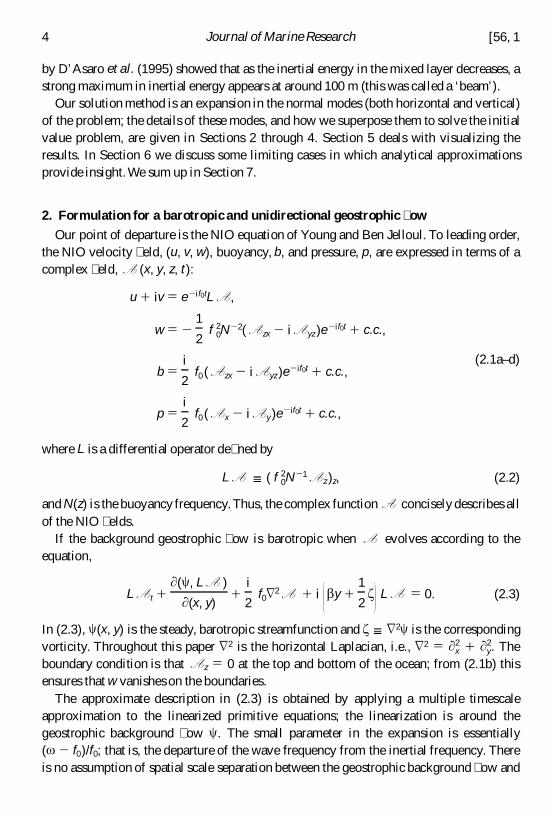
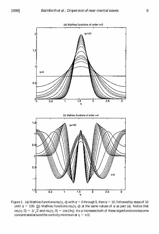
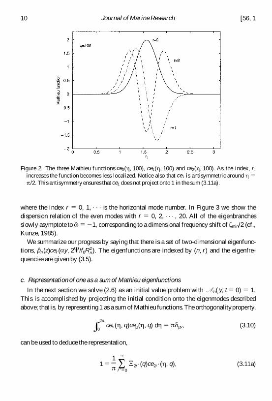
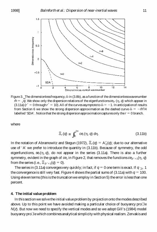
where
J r (q) e 0
2 pcer ( h q) d h (311b)
In the notation of Abramowitz and Stegun (1972) J r(q) 5 A 0r (q) due to our alternative
use of lsquoArsquo we prefer to introduce the quantity in (311b) Because of symmetry the oddeigenfunctions ser( h q) do not appear in the series (311a) There is also a furthersymmetry evident in the graph of ce1 in Figure 2 that removes the functions ce2r8 1 1( h q)from the series (ie J 2r8 1 1(q) 5 0)
The series in (311a) converges very quickly in fact if q 5 0 one term is exact If q frac34 1the convergence is still very fast Figure 4 shows the partial sums of (311a) with q 5 100Using eleven terms (this is the truncation we employ in Section 5) the error is less than onepercent
4 The initial value problem
In this section we solve the initial value problem by projection onto the modes describedabove Up to this point we have avoided making a particular choice of buoyancy pro leN(z) But now we need to specify the vertical modes and so we adopt Gillrsquos (1984) modelbuoyancy pro le which combines analytical simplicity with physical realism Zervakis and
Figure 3 The dimensionless frequency v ˆ in (38b) as a function of the dimensionlesswavenumberm 5 Icirc q We show only the dispersion relations of the eigenfunctions ce2r8( h q) which appear in(311a) (r8 5 0 through r8 5 10)All of the curves asymptote to v ˆ 5 2 1 In anticipationof resultsfrom Section 6 we show the strong dispersion approximation as the dashed curve v ˆ 5 2 m24labelled lsquoSDArsquo Notice that the strong dispersionapproximationcaptures only the r 5 0 branch
1998] 11Balmforth et al Dispersion of near-inertial waves
Levine (1995) provide some useful additional information concerning the properties ofthese vertical modes
a Gillrsquos buoyancy pro le
Gillrsquos buoyancy pro le is
N (z) 5 50 if 2 Hmix z 0
s(z0 2 H 2 z) if 2 H z 2 Hmix(41)
(Gill placed z 5 0 at the bottom of the ocean we prefer to use the convention that z 5 0 isthe surface of the ocean) Typical values for the parameters are given in Table 1 Asmentioned in Section 2 there is a set of Sturm-Liouville eigenfunctions that satisfy
dpn
dz5 2 N 2hn cn
2dhn
dz5 pn (42ab)
where cn 5 f0Rn is the eigenspeed Gillrsquos analytic solution for hn and pn arises on solving(42ab) with (41)
Figure 5 summarizes the solution of the eigenproblem by showing qn2 5 2 C f0n 2R n2 as
a function of n Figure 5 can be used to quickly estimate the value of q which is used in thesolution of the horizontal eigenproblem (33a) For instance suppose that one is interested
Figure 4 The series in (311a) truncated after the indicated number of terms Because (311a) isrepresenting a smooth periodic function (viz one) as a superposition of smooth periodicfunctions (viz cer( h 100)) there is no Gibbsrsquo phenomenon and the error of the truncated sumeventually decays exponentiallyas the number of retained terms increases
12 Journal of Marine Research [56 1
Table 1 Numerical values of the parameters used in the calculationsThe numerical values of C a Y and T refer to the lsquostandard casersquo of Section 5b
Quantity Symbol Typical numerical value
Ocean depth H 4200 mMixed layer depth Hmix 50 mStrati cation parameter s 25 m s2 1
Vertical scale of N z0 43296 mN at base of mixed layer Nmix 001392 s 2 1
Inertial frequency f0 10 2 4 s 2 1
Length scale of geostrophic ow a 2 1 80000 mMaximum geostrophic streamfunction C 4000 m2 s 2 1
Minimum geostrophic vorticity z min 5 2 4 a 2C 2 25 3 10 2 6 s 2 1
Kinetic energy density K 5 (a C )2 1400 m2 s2 2
Time scale T 5 2 z min 926 daysNondimensionalocean depth H 83Nondimensional strati cation parameter micro 0139Nondimensionalgeostrophic ow strength Y 3302Normalization constant N 1200
Figure 5 A plot of 2 C n 2R n2 f0 versus vertical mode number n The modal speed cn 5 f0Rn is the
eigenvalue obtained from solving the vertical eigenproblem in (41) and (42) We use thenumerical values from Table 1 ie C 5 4000 m2 s2 1 Using the combination qn2 on the verticalaxis removes the strongest dependence on the vertical mode number
1998] 13Balmforth et al Dispersion of near-inertial waves
in vertical mode number n 5 10 and C 5 4000 m2 s 2 1 Then it follows from Figure 5 thatq(10)2 5 0115 or q 5 115 Using Figures 1 and 2 one can then get some impression ofthe structure of the horizontal modes with the common vertical mode number n 5 10
The eigenmodes in (42a) are orthogonal
e 0
Hpn (z)pm(z) dz 5 (Hmixs n )d mn e 0
HN 2 (z)hn(z)hm(z) dz 5 (Hmixcn
2 s n ) d mn (43ab)
where the normalization constant s n is de ned in Eq (A9) of Gill3
b The vertical structure of the initial condition
Gill considered an initial condition in which the mixed layer moves as a slab Here weuse a modi ed form of Gillrsquos initial condition Speci cally we take
uI(z) Sn 5 1
80
e ns npn (z) e n N exp ( 2 n 2600) (44ab)
and vI(z) 5 0 The normalization factor N in (43b) is computed to ensure that uI(0) 5 1The initial condition (43) is shown in Figure 6 As a result of truncating the sum at n 5 80and including the low pass lter e n there is now some initial excitation in about the rst 20
3 There is a misprint in (A9) of Gill With the notation of that Appendix the expression for s n should be
s n 5 2 e 1 1 1e
22 m 2 5 1 m 2 11
42 [ e 1 j T (1 1 e 2m 2 )] 62 1
Figure 6 The initial velocity uI(z) and the initial shear duI(z)dz (solid and dashed respectively)calculated from (44) The highest vertical eigenmode n 5 80 is shown in the left-hand portion ofthe gure The function p80(z) is shown by the solid curve and h80(z) by the dotted curve
14 Journal of Marine Research [56 1
meters below the mixed layer This is probably more realistic than a completely discontinu-ous initial condition Further since we are interested in examining the evolution of thevertical shear we must have an initial condition in which the shear is nite the initial shearpro le in Figure 6 is consistent with the observation of shear concentration at the base ofthe mixed layer
Additional motivation for the initial condition in Figure 6 is provided by the very slowconvergence of the un ltered series to Gillrsquos discontinuous initial velocity For instance ifthe un ltered series is truncated after P terms then the error is O(1P) Further the initialcondition de ned by a truncated sum exhibits Gibbsrsquo phenomenon even with P 5 120terms there is unrealistic oscillatory structure at relatively deep levels The ltering factore n eliminates this lsquolsquoringingrsquoand provides a strongly localized initial excitation
c Projection of the initial condition on the modes
We now represent A ( y z t ) as a sum of vertical normal modes as in (25) and projectthe initial condition L A ( y z 0) 5 uI(z) in (44) onto this basis set The result is that
An (y 0) 5 2 R n2e ns n (45)
Thus after the projection on vertical normal modes the problem is to solve
shy An
shy t1 2ia 2C cos (2a y) An 5
i
2 n
shy 2 An
shy y2 (46)
with the initial condition in (45)Next we use (311a) to project the initial condition (45) onto horizontal eigenmodes
This gives
An (y t ) 5 2 R n2e ns n S
r 8 5 0
`
J 2r8n exp ( 2 iv 2r8nt ) ce2r 8 (a y 2 C n ) (47)
where J 2r8n J 2r8(2 C n) The frequency of the mode with index (2r8 n) is as beforev 2r8n 5 na 2a2r8(2 C n)2
d Reconstruction of the velocity and the shear
To reconstruct the nal elds one must sum (47) over the vertical mode number nThus using (21a) with Lpn 5 2 Rn
2 2pn one nds that the horizontal velocities are given by
u 1 iv 5 e 2 if0t Sn5 1
80
Sr 8 5 0
10
e n s n J 2r 8n exp ( 2 i v 2r 8nt ) ce2r 8( a y 2C n) pn (z) (48)
The sum over r8 in (48) has been truncated after eleven terms this is more than enough toensure convergence (see Fig 4) In addition one obtains from (48) the following
1998] 15Balmforth et al Dispersion of near-inertial waves
expression for the vertical shear
uz1 ivz 5 2 e 2 if0tN 2 Sn5 1
80
Sr 8 5 0
10
e n s n J 2r 8n exp ( 2 iv 2r 8nt ) ce2r 8( a y 2 C n ) hn(z) (49)
where hn is de ned in (42) The series in (48) and (49) are our solution of the initial valueproblem posed in Figure 6
Before attemptingvisualizationof the solution let us examine the spectral decay of (48)and (49) Using the orthogonality relations in (43) the total squared velocity is
e 0
2p a
e 0
H(u 2 1 v2 ) dz dy 5 p Hmix a
2 1 Sn 5 1
80
Sr 8 5 0
10
e n2s nJ 2r 8n
2 (410)
from which we can read off the fraction of energy contained in the mode (r8 n)
E2r 8n e n2s nJ 2r 8n
2 Y Sn5 1
80
Sr 8 5 0
10
e n2 s n J 2r 8n
2 (411)
This modal energy fraction is shown in Figure 7aThe modal content of the total squared shear is a little more difficult to estimate because
the functions N 2 n(z) are not orthogonal Hence the total square shear
e 0
2p a
e 0
H(u z
2 1 v z2 ) dz dy (412)
does not separate into a convenient sum over squares of modal amplitudes However theorthogonality relation (43b) shows that the functions Nhn(z) are orthogonal Hence weestimate the modal content of the mean square shear using the weighted average
e 0
2p a
e 0
HN 2 2 (u z
2 1 v z2 ) dz dy (413)
Thence the fraction of the weighted mean square shear in the mode (r8 n) is given by
S2r8n e n2s nJ 2r 8n
2 c n2 2 Y Sn 5 1
80
Sr 8 5 0
10
laquo n2 s n J 2r 8n
2 c n2 2 (414)
which is shown in Figure 7b Notice that the expression in (413) is proportional to anlsquoinverse Richardson numberrsquo averaged over the volume of the uid Thus S2r8n in (414) isthe contributionof mode (2r8 n) to the inverse Richardson number
Figure 7 shows that the truncation in (48) is sufficient to resolve both the velocity andshear The velocity is heavily concentrated in the low modes In particular the modes withhorizontal mode number r 5 0 contain over 85 of the energy On the other hand the shearis distributed more evenly over higher modes (note the different scales of the vertical axesin the two parts of Fig 7)
16 Journal of Marine Research [56 1
Another view of the initial excitation is shown in Figure 8 where E2r8n is plotted againstthe dimensionless modal eigenfrequency v ˆ in (39) It is signi cant that the eigenfrequen-cies with v ˆ lt 2 1 (that is dimensional frequencies close to z min2) do not contain muchenergy This might bear on DrsquoAsarorsquos (1995b) unsuccessful attempt to observe a z 2frequency shift using the Ocean Storms data set Our model initial condition simply doesnot excite modes with eigenfrequencies close to z min2 In fact the concept of a spatiallylocal frequency shift is usually meaningless when one has eigenmodes The conceptacquires some meaning if the eigenmodes are spatially localized near a potentialminimum
Figure 7 (a) Upper panel the fraction of energy E2r8n in (411) in the mode (2r8 n) Notice that theaxis is r 5 2r8 Most of the energy is contained in the rst two horizontal modes with r8 5 0 andr8 5 1 (b) Lower panel the fraction of square shear (or inverse Richardson number) S2r8n in(414) in mode (2r8 n) Note the different scales on the vertical axes in (a) and (b) As expectedhigher modes make a more important contribution to the shear
1998] 17Balmforth et al Dispersion of near-inertial waves
this is why the eigencurves in Figure 3 asymptote to v ˆ 5 2 1 (corresponding to z min2) Butto strongly excite such localized modes we would need a very different initial condition
5 Results
a Dimensional considerations
To systematically discuss the results of parametric variations we must rst consider thenondimensional form of the problem As nondimensional independent variables we use
t tT h a y z 5 (z 1 Hmix)Hmix (51)
where following our earlier de nition of the nondimensional frequency in (38b) thetimescale is T 5 2 z min For the sinusoidal ow in (31) this choice of T is equivalent to
T 1
2 a 2 C (52)
The nondimensional vertical coordinate is 2 H z 1 where the nondimensional oceandepth is H (H 2 Hmix)Hmix Notice that z 5 0 is the base of the mixed layer and z 5 1 isthe ocean surface The buoyancy frequency can be measured in units of its value directly
Figure 8 The fraction of energy in mode (2r8 n) E2r8n in (411) plotted against the nondimensionalmodal frequency 2 v 2r8nz min The horizontal axis is truncated at v ˆ 5 25 there are higherfrequencies in the series (48)
18 Journal of Marine Research [56 1
beneath the mixed layer Nmix for the particular pro le of (41) we then nd
N (z) 5 50 if 0 z 1
1(1 2 2microz) if 2 H z 0(53)
where micro Hmix2(z0 1 Hmix 2 H ) and Nmix s(z0 2 H 1 Hmix)The nondimensional form of the A equation can then be written
Y [L A t 1 i cos 2 h L A ] 1 i A h h 5 0 (54)
where L is the nondimensional differential operator
L 5 shy z N 2 2 shy z (55)
The most important nondimensionalparameter in the problem is
Y 4C f0
Hmix2 Nmix
2 (56)
Y is a measure of the strength of the geostrophic ow speci cally Y z minV where V a 2Hmix
2 Nmix2 f0 is the back-rotated frequency of a wave whose horizontal scale is that of the
geostrophic ow and whose vertical scale is the mixed layer depthThe solution of the initial value problem is discussed mainly using dimensional
variables However the considerations above show that there are only three independentnondimensional parameters viz micro H and Y In fact of the parameters in the barotropicstreamfunction C and a the length scale a 2 1 appears only in the time scale T Hencechanges in the strength of background ow are made by modifying C which is equivalentto changing Y
b The standard case
We now examine the temporal behavior of the solution for a particular selection ofmodel parameters which we refer to as the lsquostandardrsquocase (we use the label S to signify thiscase in subsequent gures) these choices are listed in Table 1 Figures 9ndash11 summarize theresults because Y 5 3302 (corresponding to a peak velocity of 10 cm s 2 1) the standardcase has a fairly strong background ow
In Figure 9 we show how the lsquospeedrsquo Icirc L A L A 5 Icirc u2 1 v 2 evolves in timeInitially the speed is sharply concentrated in and just below the mixed layer (see Fig 6)But after 10 days (Fig 9a) the development of both horizontal and vertical structure isevident
In the mixed layer itself the sinusoidal barotropic ow (c z ) ~ cos 2h impresses ananalogous modulation cos 2h on the NIO speed In fact the modulation is so strong that itincreases the speed by about 20 over its initial value in the vicinity of the vorticityminima ( h 5 p 2) The structure is very different directly below the mixed layer Enhanced
1998] 19Balmforth et al Dispersion of near-inertial waves
downward propagation is correlated with both the maxima and the minima of the vorticitythis results in a second harmonic cos 4 h structure in the NIO speed below the mixed layer
In some respects these patterns agree with the observations described by van Meurs(1998) First the rate at which near-inertial activity lsquodisappearsrsquo from the mixed layer isspatially inhomogeneousvan Meurs observed that the time scale varied between 2 and 20
Figure 9 Panels (a)ndash(f) show snapshots of the speed L A ( y z t ) 5 Icirc u2 1 v 2 as surface plotsabove the ( h z) plane every 10 days after the initiation of the near-inertialoscillationThe depth zis in meters and h 5 2 a y is dimensionless
20 Journal of Marine Research [56 1
days depending on locationvan Meurs also attempted to correlate the energy level with thegeostrophic vorticity Figure 9a suggests that in the mixed layer there is a strongcorrelation high NIO energy with negative vorticity (eg h 5 p 2) and low NIO energywith positive vorticity (eg h 5 0 and p ) Such a correlation was not seen unambiguouslyin van Meursrsquos drifter observations It may be that the mesoscale vorticity is not wellresolved by this data set Alternatively if some of the drifters happened to be drogued to uid beneath the mixed layer then those drifters would see elevated energy levels at boththe maxima and minima of the vorticity (as in Fig 9a)
By 20 days the spatial pattern is even clearer (Fig 9b) Notice that near the vorticitymaxima ( h 5 0 and p ) the speed now has a submixed-layer maximum In other words itappears as though the near-inertial energy has been expelled from the mixed layer at h 5 0and p and concentrated just below the base of the mixed layer These concentrations ofactivity subsequently propagate horizontally (Figs 9bndash9e) and add to downwardly propa-gating oscillations from the mixed layer near h 5 p 2 This results in the formation of asubstantial peak in speed just below the mixed layer at the vorticity minima ( h 5 p 2)
Over this period the activity in the mixed layer near the vorticity minimum begins todecline Eventually in Figures 9dndashf the near-inertial activity disperses downward At thevorticity minimum ( h 5 p 2) the mixed-layer speed nally falls below its initial level By60 days activity remains peaked below the mixed layer at the vorticity minimum and verydeep penetrationof near-inertial activity takes place only in regions of positive vorticity (inFig 9f near h 5 0 and p the speed is fairly uniform over the top 1000 m)
More quantitative features of the solution are shown in Figures 10 and 11 Figure 10shows the backrotated velocity eld below both the maximum (Fig 10a) and the minimum(Fig 10b) of the vorticity The contours in Figure 10 are curves of constant speed Bothparts of Figure 10 show the formation of what DrsquoAsaro et al (1995) call a lsquolsquobeamrsquorsquo InFigure 10b the lsquolsquobeamrsquorsquo is composed of strong inertial currents below the mixed layer andis located roughly in the region between z 5 2 50 m and z 5 2 100 m In fact as thecontour labelled 125 indicates the speed can be larger than that of the initial conditionThe lsquolsquobeamrsquorsquo is also apparent though less intense in Figure 10a
Figure 11 shows the backrotated shear vectors below the maximum (Fig 11a) andminimum (Fig 11b) of the vorticity Because the shear eld is shallower and has moresmall-scale structure than the velocity eld we have changed the depth scale relative tothat of Figure 10 We have also not shown the mixed layer (where the shear is zero) Thereare interesting qualitative differences between Figure 11a and 11b (The differences aregreater than those between Figs 10a and 10b)
c Parametric variations
As gross indications of how changes in the parameters alter the evolution we use twoaveraged measures of the inertial activity in the mixed layer
1998] 21Balmforth et al Dispersion of near-inertial waves
Figure 10 Temporal evolution of the backrotatedvelocity eld (u v) with depth z (meters) at (a) thevorticity maxima (h 5 0 p ) and (b) the vorticity minima (h 5 p 2 3 p 2 ) Shown arethe backrotated velocity vectors at the points (t z) The contours are curves of constant speed
Icirc u 2 1 v2 The initial speed in the mixed layer is 1 and the contour interval is 02
22 Journal of Marine Research [56 1
Figure 11 Temporal evolution of the backrotated shear eld (uz vz) with depth z (meters) at (a) thevorticity maxima (h 5 0 p ) and (b) the vorticity minima (h 5 p 2 3 p 2 ) Note Thedepth scale in this gure differs from that of Figure 10 Shown are the backrotated shear vectors at
the points (t z) The contours are curves of constant shear strength Icirc u z2 1 v z
2 In the initialcondition the shear has a maximum value of 514
1998] 23Balmforth et al Dispersion of near-inertial waves
First from (311a) and (47) we obtain the horizontally averaged velocity
7 u 1 iv8 a
p e 0
p a(u 1 iv) dy
51
2 pe 2 i f0t S
n 5 1
80
Sr 8 5 0
10
e n s n exp ( 2 iv 2r 8nt ) J 2r 8n2 pn(z)
(57)
In the mixed layer the expression above simpli es because pn(z) 5 1 Thus one measureof inertial activity obtained from (57) with pn 5 1 is the magnitude of the horizontallyaveraged mixed-layer velocity that is Icirc 7 u 8 2 1 7 v 8 2
Our second measure of near-inertial activity uses the shear The horizontal average ofthe shear is from (48)
7 uz 1 ivz 8 5 21
2 pe 2 if0tN 2 S
n 5 1
80
Sr 8 5 0
10
e ns nJ 2r 8n2 exp ( 2 iv 2r 8nt ) hn(z) (58)
from which we may construct the magnitude Icirc 7 uz8 2 1 7 vz 8 2 at a depth of 51 m This depthone meter below the base of the model mixed layer is very close to where the initial shearin Figure 6 achieves its maximum value
Suppose that the parameters de ning the sinusoidal ow in (31) are varied by changingboth a and C so that the timescale T in (52) is xed at the value of the standard casenamely T 5 926 days Figure 12a then shows the decrease of Icirc 7 u 8 2 1 7 v 8 2 versus t 5 tT at ve different values of Y Figure 12b shows the variation of Icirc 7 uz 8 2 1 7 vz 8 2 at the base of themixed layer in the same ve cases The trend in Figure 12 is clear increasing Y in (54)while holding T 5 2 z min xed enhances the decay of mixed-layer speed and shear(though the shear is less sensitive to changes in Y than the speed)
The parameter Y is the most important nondimensional group controlling the decay rateof inertial activity in the mixed layer the results in Figure 12 are insensitive to changes inthe other two nondimensionalparameters micro and H of (53) For example for the parametervalues summarized in Table 2 Y and T are xed but the strati cation parameters arealtered by factors of over two Figure 13 shows the decay of Icirc 7 u 8 2 1 7 v8 2 in these differentcases the decay is clearly similar for all four4
The horizontal modulation of the NIO is also strongly dependent on changes in Y Toillustrate this behavior consider the three calculations in Figure 12a with Y 5 3302 1651and 0413 at the times when Icirc 7 u 8 2 1 7 v 8 2 5 054 in the mixed layer For the standard casethis is at t 5 30 days or tT 5 324 and Figure 9c shows a snapshot of the speed Icirc u 2 1 v 2
4 In view of the sensitivity in Figure 12 the collapse of the four curves in Figure 13 is impressive but notperfect The differences which remain in Figure 13 are due to two effects The most important is that the lteringfactor exp ( 2 n2600) in (43b) is not changed when the parameters are varied Thus in terms of thenondimensional coordinate z in (51) the four cases have slightly different initial conditions Second because ofthe large differences in H the lowest vertical modes have signi cantly different frequencies this producesidiosyncratic lsquowigglesrsquo such as the large dip on curve B at around tT 5 8
24 Journal of Marine Research [56 1
Figure 12 (a) Evolution of the speed Icirc 7 u8 2 1 7 v8 2 or the horizontally averaged velocity 7 u 1 iv 8de ned in (57) The value of Y in the ve different curves is indicated beside each curve The casewith C 5 4000 m2 s2 1 or Y 5 3302 is the standard case shown in Figures 9 through 11 Thehorizontal axis is in units of tT where T 1(2a 2C ) (b) Temporal evolution of the magnitude of
the shear of the horizontally averaged ow Icirc 7 uz 8 2 1 7 vz 8 2
as a surface plot above the ( h z) plane Figure 14 shows the analogous surface plots for theother two calculationswith smaller values of Y As Y is reduced the horizontal modulationof the NIO elds become weaker (The strong dispersion approximation of Young and BenJelloul (1997) is valid in the case Y frac12 1 the leading order term of this approximation isthat A is independent of the horizontal coordinates Figure 14b is approaching thisweakly modulated state)
d Radiation of a near-inertial wave train
In the standard case the solution develops what we have termed a lsquolsquobeamrsquorsquo (followingDrsquoAsaro et al 1995) This is the shallow concentration of energy which rst appears
Table 2 Four parameter settings all with Y 4C f0(NmixHmix)2 5 3302 and all with the sametimescale T 5 1(2a 2 C ) 5 926 days S denotes the standard case from Table 1 The buoyancypro le is speci ed by giving (H Hmix z0 Nmix) and then the strati cation parameter s in (41) iscalculated from s 5 Nmix[z0 2 H 1 Hmix] In all four cases H 5 4200 m and z0 5 43296 m
Case C (m2 s2 1) a 2 1 (km) Nmix (s 2 1) Hmix (m) micro H s (m s2 1)
S 4000 80 001392 50 01392 83 25000A 1000 40 001392 25 00808 167 21520B 1000 40 0009843 3535 01071 1178 16236C 4000 80 0006960 100 02178 41 15980
Figure 13 Evolution of the speed Icirc 7 u 8 2 1 7 v 8 2 for the four parameter sets (A B C and S) inTable 2 Y 5 3302 in all cases while micro and H have large variations
26 Journal of Marine Research [56 1
below the base of the mixed layer at the vorticity maximum and then moves horizontally tothe vorticity minimum (see Fig 9) We stress that the vertical propagation of the beam ismodest the maximum in near-inertial energy is concentrated just below the base of themixed layer (see Fig 10) The phenomenon occurs at depth between 50 and 100 m
Another interesting phenomenon which occurs at a different parameter settings (name-ly when 03 Y 1) is illustrated in Figure 15 a train of near-inertial waves is radiatedfrom the mixed layer into the deeper ocean Because the train is con ned to theneighborhood of vorticity minimum it has a relatively small horizontal length scale Incontrast to the beam the near-inertial wavetrain has a substantial vertical propagation
The wavetrain is evidently a phenomenon in which the modes of the system are acting inconcert to produce local vertically propagating wave packets In fact the horizontallocalization of the train near the vorticity minimum is explained by Kunzersquos ray-tracing
Figure 14 Snapshots of the speed L A ( y z t ) 5 Icirc u 2 1 v 2 as a surface plot above the (h z)
plane The two calculations above and the one in Figure 9c all have Icirc 7 u8 2 1 7 v8 25 054 in themixed layer The value of Y and the nondimensional time is indicated on the gure As Y isincreased the horizontal structure of the elds becomes more complex When Y is small as inFigure 14b the relatively weak horizonal modulations indicate that the strong dispersionapproximation of Section 6 is valid
1998] 27Balmforth et al Dispersion of near-inertial waves
arguments Equivalently the Mathieu modes of Figures 1 and 2 tend to be trapped aroundthe vorticity minimum at h 5 p 2 More precisely from the Mathieu equation (33) thereare turning points at the values of h determined by a 2 2q cos 2 h 5 0 or equivalently2 v 5 z min cos 2 h In the vicinity of the vorticity minimum bounded by these points wavesmay propagate vertically they are evanescent elsewhere This explains qualitatively whythe wavetrain arises at the vorticity minimum and not at the maximum
A second argument follows from considering an effective group velocity Because most
Figure 15 An illustration of the radiation of a near-inertial wave train from the mixed layer (a)Speed as a functionof depth (meters) and time (days) below the vorticity maxima h 5 0 and p (b)Speed as a function of depth and time below the vorticity minima h 5 p 2 The wave train isapparent only below the vorticity minimum (c) Another view of the near-inertial activity belowthe vorticity minimum the arrows indicate the backrotated velocity L A 5 exp (if0t )(u 1 iv)superposed on a depth-time plot The solid curve is the trajectory in (512) Notice the reversal indirection with depth of the near-inertialvelocity
28 Journal of Marine Research [56 1
of the energy is contained in the Mathieu mode with r 5 0 we use the nondimensionaldispersion relation in (39) and consider only the zeroth eigenmode Figure 16 shows thenondimensional frequency and group velocity
v ˆ 5 a0 (m 2)2m 2 and v ˆ m 5 [m 2 1a08 (m 2 ) 2 m 2 3a0 (m 2)] (59ab)
as functions of m The crucial point is that the group velocity has a minimum (ie mostnegative) value at m p 10 In terms of dimensional variables the extremum is at
m p Icirc N 22 C f0 (510a)
and the minimum group velocity is
cg 2 038a 2 C Icirc 2 C f0
N 2 (510b)
the frequency at m 5 m p is
v p 2 024a 2 C (510c)
Figure 16 The dimensionless frequency v ˆ (the dashed curve) in (38b) as a function of thedimensionless vertical wavenumber m in (38a) Only the r 5 0 branch from Figure 3 is shownAlso shown is the dimensionless vertical group velocity v ˆ m (the solid curve) The vertical groupvelocity has an extremum at around m 5 10
1998] 29Balmforth et al Dispersion of near-inertial waves
As an application of these results one can calculate the position of the front of thewavetrain in Figure 15 by integrating
dz
dt5 cg (z) (511)
where the dependence of cg on z arises because N(z) is given by (41) On using the initialcondition z(0) 5 2 Hmix one nds that
z(t ) 5 (z0 2 H ) 1 (H 2 Hmix 2 z0 ) exp [038a 2(2 C )32f 012s 2 1t] (512)
The trajectory in (512) is plotted in Figure 15c and gives an indication of the location ofthe front of the wavetrain
It is interesting that the vertical group velocity in (510b) is proportional to N 2 1 Thisexplains the acceleration with depth of the front of the wavetrain in Figure 15c (the frontgoes faster as N decreases) The standard internal wave dispersion relation has the oppositetendencywith xed k and m the vertical group velocity of internal waves in a resting ocean( C 5 0) decreases as N decreases
Wavetrains like that of Figure 15 occur only if Y is neither too small nor too largeRoughly speaking if N(z) is speci ed using the parameters in Table 1 then trains areprominent over the range 03 Y 1 To rationalize this dependence on Y notice that ifY ~ C reg 0 then the wavenumber m p in (510a) becomes large the maximum groupvelocity occurs at high vertical wavenumbers which are not initially excited On the otherhand if Y frac34 1 then m p becomes small the maximum group velocity approaches smallvertical mode numbers and eventually certainly before m p
2 1 H there is no longer aneffective continuum of modes In this case the concept of a group velocity is meaninglessand in numerical calculations we observe little coherent vertical propagation but rathersubstantial horizontal modulation
6 Limiting cases
Throughout this paper we have con ned attention to the sinusoidal ow in (31) Thisnarrow focus has enabled us to obtain a detailed picture of the radiation of a large-scalenear-inertial excitation Now we consider two limiting cases Y frac12 1 and Y frac34 1 in whichinsight can be obtained by analytical considerations
a Strong dispersion Y frac12 1
The case Y frac12 1 corresponds to the strong dispersion approximation of Young and BenJelloul (1997) The validity of strong dispersion requires C f0R n
2 frac12 1 For the low modeswith Rn 10 km C f0R n
2 is small But because Rn reg 0 as n increases the strong dispersionapproximation fails for sufficiently high vertical modes We can better appreciate the utilityof the approximation by applying it to the speci c problem we have solved in this paper
In the present context the strong dispersion approximation is a perturbative solution of
30 Journal of Marine Research [56 1
the nondimensional A -equation (55) in the case Y frac12 1 By expanding A 5 A0 1Y A1 1 middot middot middot one nds that the leading order is just A0h h 5 0 that is horizontal wavedispersion dominates The solution of the leading order problem is therefore
A0 5 A0(z t) (61a)
In Appendix B the expansion is carried to higher order the nal result in dimensionalvariables is an evolution equation for B L A0
Bt 1 if 02 1KL B 5 0 (61b)
where K a 2C 2 is the average kinetic energy density of the sinusoidal ow (31) Thedispersion relation obtained from (61b) is the parabola v ˆ 5 2 m24 labelled lsquoSDArsquo inFigure 3
In the strong dispersion approximation the small parameter Y multiplies the terms withthe most z-derivatives in (55) this hints that the expansion in (61) is not uniformly validfor the high vertical modes This nonuniformity can be assessed more precisely byreturning to the horizontal eigenproblem the Mathieu equation in (33a) and noting thatthe strong dispersion approximation is equivalent to using the q frac12 1 expansion of the r 5 0eigenfunction ie
ce( h q) 51
Icirc 2 3 1 2q
2cos 2 h 1 O (q 2) 4 (62)
On referring to Figure 1a we see that if q frac12 1 then the eigenmodes have weak horizontalmodulation But because q 2C n n2 (see Fig 5) the expansion is invalid as n reg `with C xed
Because the strong dispersion approximation fails for sufficiently high vertical modenumber n its validity is determined by how strongly the initial condition excites modeswith n frac34 1 Moreover the strong dispersion approximation lters all of the horizontalmodes with r $ 2 Hence we also require a weak excitation of these more complicatedhorizontal structures
We make a pragmatic assessment of the approximation by tolerating a fractionalfrequency error of about 03 That is referring to Figure 3 let us say that the strongdispersion approximation is acceptable if
q 5 m 2 2 (63)
(Because a0(2) 5 151395 the error in the SDA eigenfrequency is 32 at q 5 2) Given(63) and the de nition q 2 C f0Rn
2 we can plot the curve C 5 f0Rn2 (equivalently q 5 2)
in the (n C ) plane see Figure 17 In the region below the curve we decree that theapproximation is acceptable
Also superposed on Figure 17 is the cumulative fraction of energy which is contained inmodes with vertical mode number less than or equal to n That is because s n e n
2 is the
1998] 31Balmforth et al Dispersion of near-inertial waves
fraction of energy in vertical mode number n the right-hand axis shows
Cn Sj5 1
n
e n2 s n (64)
as a function of n The two parts of Figure 17 are for different values of HmixGiven the value of C we read off the number of modes that are acceptably approximated
by strong dispersion and also the amount of energy contained in them For example withC 5 2000 m2 s 2 1 the accurately approximated modes are those with n 6 These modescontain 80 of the energy if Hmix 5 50 m but only 65 if Hmix 5 25 m Provided that the
Figure 17 The gure above can be used to estimate the fraction of the energy which is contained inmodes which are acceptablydescribed by the strong dispersionapproximationsThe solid curve isq 5 2 (that is C 5 f0 n
2 ) as a function of the vertical mode number n This curve depends on theparameters used to specify the model buoyancy pro le in (41) shown above are two exampleswith different values of Hmix as indicated (The other parameters are given in Table 1) The circlesand right-hand ordinate show the cumulative fraction of energy contained in modes with verticalmode number less than or equal to n
32 Journal of Marine Research [56 1
fraction of energy contained in these lsquolsquostrongly dispersingrsquorsquo modes is sufficiently large wehave some grounds for making the approximation Accordingly we might expect theapproximation to be adequate in the former example less so in the latter
Hence if we insist that 80 of the energy must be contained in the strongly dispersingmodes in order to use the approximation then this restricts us to the parameter regime C 2000 m2 s 2 1 if Hmix 5 50 This range is sufficiently wide to make the approximation arelatively useful tool in more complicated situations
As an example of the application of the approximation the solution of (61b) with theinitial condition in Figure 6 is
L A0 5 Sn 5 1
80
s ne npn (z) exp 1 iKt
n 2 (65)
Figure 18 shows a comparison between the approximate solution in (65) (the dotted curve)and the full numerical solutionsThe standard case which has Y 5 3302 is labelled by lsquoSrsquoThe other solid curves in Figure 18 are obtained by varying C and therefore Y by factorsof 2 while also adjusting a so that the kinetic energy density K 5 a 2 C 2 is xed Figure 18shows that the standard case is not well approximated by (65) but that if Y 5 1651( C 5 2000) is less there is agreement
Figure 18 Comparison of the speed of the average velocity in the mixed layer (de ned in (57) withpn(z) 5 1) calculated with the strong dispersion approximation (65) with that obtained from thefull series expansion in (48) The results from (48) are the solid curves and the standardcase fromTable 1 is labelled lsquoSrsquo The other four solid curves are obtained by varying C by factors of 2 withthe kinetic energy density K 5 a 2 C 2 xed The value of C is indicated in three cases eg for thestandard case C 5 4000 m2 s2 1 The approximation (65) is the dotted curve
1998] 33Balmforth et al Dispersion of near-inertial waves
One interesting point apparent from (65) from Figure 18 and also from the multipletime scale expansion in Appendix B is that in the strong dispersion regime the relevantevolutionary time scale is
T
Y5
1
8
Nmix2 Hmix
2
f0K (66)
Notice that T Y depends only on the combination K 5 C 2 a 2 (not on C and a separately)This explains the condensation of the solid curves in Figure 18 as Y is reduced with K xed once one enters the strong dispersion regime the rate of decay of mixed layer speed isinsensitive to further reductions in Y
b Strong trapping Y frac34 1
When Y is large we may again simplify (54) by asymptotic means We proceed byde ning a small parameter e 5 Y 2 14 Next we observe that for a xed mixed layerstructure (constant Hmix and Nmix) q ~ Y where q is the Mathieu parameter in (33) Hencein this limit q frac34 1 and the Mathieu modes into which we decompose the initial conditionare localized (or lsquostrongly trapppedrsquo) near the vorticity minimum at h 5 p 2 (see Section 3and Fig 1) This guides us to introduce a rescaling of the horizontal spatial coordinate
h 5p
21 e j (67)
We further de ne multiple timescales such that
shy t reg shy t 1 e 2 shy t (68)
The governing equation is then
L At 1 e 2LAt 1 i cos ( p 1 2 e j ) L A 1 ie 2 A j j 5 0 (69)
On introducing the asymptotic sequence A 5 A0 1 laquo A1 1 we nd at leadingorder
L A0t 2 iL A0 5 0 (610)
Without loss of generality we solve (610) with
A0 5 e it C ( h z t ) (611)
where C is an as yet undetermined functionThe physical content of (611) is that at leading order the wave frequency is shifted by
z min2 indeed because the modes are strongly trapped Kunzersquos ray tracing approximationis applicable in this limit However the small parameter in this approximation is e 5 Y 2 14
and because of the small power it is difficult to access this asymptotic regime with oceanicvalues
34 Journal of Marine Research [56 1
At order e 2 we obtain
L A1t 2 iL A1 1 LA0 t 1 ij 2
2L A0 1 i A0j j 5 0 (612)
The terms in A1 will lead to secularly growing solutions on the fast timescale t unless theterms containing A0 cancel This leads to
LC t 1 ij 2
2LC 1 iC j j 5 0 (613)
The vertical transmission of the disturbance is therefore described by the solvabilitycondition (613) That is vertical propagation occurs on the timescale t 5 t Y Icirc Y Onrestoring the dimensions the dimensional timescale is
T1 5 Y 2 12T HmixNmix
4 a 2C 32f 012
(614)
Evidently the larger the Y the smaller the T1 and so the energy disperses faster out of themixed layer as one increases the strength of the geostrophic ow
Figure 19 Speed averaged in the mixed layer against the scaled time tT1 where T1 is de ned in(614) for ve calculations with Y 5 1651 3302 6604 1321 and 2642 Hmix and Nmix are as inthe standard case
1998] 35Balmforth et al Dispersion of near-inertial waves
In Figure 19 we display the speed average in the mixed layer plotted against the scaledtime tT1 for various values of Y 1 Relative to Figure 12 the curves collapse rathermore closely to a common behavior we take this as con rmation that the dominant decaytimescale is T1 when Y frac34 1
7 Discussion and conclusion
In this paper we have given a detailed solution of an idealized problem which modelsthe vertical transmission of near-inertial activity Despite the many simpli cations themodel does represent some realistic features For instance in response to the questionsposed in the introduction the solutions show the way in which a pre-existing geostrophic ow creates horizontal modulations in an initiallyuniform NIO (eg Fig 9) The solutionsalso show the formation of a lsquobeamrsquo of near-inertial energy below the mixed-layer (cfDrsquoAsaro et al 1995)
Given these qualitative successes in this conclusive section a quantitative comparisonof our results with observations such as the Ocean Storms Experiment (DrsquoAsaro et al1995) is in order However such a comparison is not straightforward One issue which hasfocussed research in this area for many years is the rate at which near-inertial activitydisappears from the mixed layer after impulsive excitation The model shows that therelevant time-scale depends on the value of the nondimensional group Y in (54) Thestrong dependence of Y on the spatially variable and subjectively determined parametersHmix and Nmix makes decisive conclusions difficult
Setting aside the problem of determining Hmix and Nmix it is next necessary to appreciatesome of the caveats of our model We assume a simple steady barotropic ow andconsider linear near-inertial oscillations we restrict attention to two-dimensional owsand ignore the effect of b Even within the limited arena of idealized two-dimensionalproblems we have used a streamfunction with a single sinusoid which has the unrealisticfeature that the wavenumber which contains all the energy is also the wavenumbercontaining all the vorticity
Given all these lacunae we can hope for no more than order of magnitude agreementbetween our model and observations Nonetheless we now attempt a comparison withOcean Storms First we must assign lsquolsquoobservational valuesrsquorsquo to C and a of the modelstreamfunction c 5 2 C cos (2 a y) DrsquoAsaro et al state that most of the kinetic energy iscontained in features with approximately the Rossby radius scale that is 40 km Accord-ingly we take
2 a 51
40 km (71)
DrsquoAsaro et al also state that the RMS eddy velocity is URMS 5 0053 m2 s 2 1 Thus froma C 5 URMS Y Icirc 2 we obtain
C 5 3000 m2 s 2 1 (72)
36 Journal of Marine Research [56 1
Given C and a we can now determine the minimum vorticity and the time scale T 52 Y z min in the model
z min 5 1874 3 102 6 s 2 1 T 5 1235 days (73ab)
To estimate Y we take Hmix 5 30 m and Nmix 5 0012 s 2 1 and we then nd Y 5 10 Hencefrom Figure 12a we estimate that to reduce the average speed to 03 of its initial level (thatis the energy to 10 of its initial level) one must wait for around t 5 3T or 37 days Thistimescale is rather long but there are greater uncertainties in both the model and theobservational parameters
For example in calculating the model parameters above we are led to an unavoidableinconsistency with the observations The observed eddy vorticity has an RMS value of0023f lt 246 3 102 6 s 2 1 and the observed z min is greater by a factor of three than theobserved RMS vorticity The model evidently does not have enough adjustable parametersto t the observed spatial scales the kinetic energy level the RMS vorticity and theminimum vorticityTo determine roughly how much the failure of the model may affect ourpredictions we calculate T directly from the observed vorticity z min lt 72 3 10 2 6 Thisgives T lt 32 daysmdashshorter by a factor of 4 than (73b) If we further take the value (72)for C we nd that the mixed layer energy falls to within 10 of its initial level after only96 days which is well within the observational constraints In view of the manyde ciencies of the model we therefore regard our study as an encouraging success
Acknowledgments This research was supported by the National Science Foundation (GrantOCE-9616017)NJB thanks the Green Foundation for generoussupport SGLS is a grateful recipientof a Lindemann Trust Fellowship
APPENDIX A
Near-inertial waves with k 5 0
The primitive equations for zonally-uniform disturbances on a unidirectional barotropic ow with streamfunction c ( y) and vorticity z 5 c yy are
ut 1 fev 5 0 vt 2 fu 1 py 5 0 pz 2 b 5 0
vy 1 wz 5 0 bt 1 wN 2 5 0(A1andashe)
where
f 5 f0 1 b y fe f0 1 b y 1 z (A2)
One can eliminate all variables in favor of v to obtain
Lvtt 1 ffeLv 1 f 02vyy 5 0 (A3)
where L is the differential operator in (22) By projecting (A3) on the vertical normalmodes in (24) we nd the Klein-Gordon equation
vntt 1 ffevn 2 cn2vnyy 5 0 (A4)
where cn 5 f0Rn is the modal speed
1998] 37Balmforth et al Dispersion of near-inertial waves
If b 5 0 and c ( y) is the sinusoid in (31) then we can look for horizontal modes byintroducing
vn (y t ) 5 Vn (y) exp [ 2 i( f0 1 v )t] (A5)
The result is the Mathieu equation
d2Vn
d h 21 (a 2 2q cos 2h )Vn 5 0 (A6)
where h 5 a y and
a 5 2 3 1 1v
2f0 4v
n a 2 q 2 C n (A7ab)
On comparing (A6) with the result obtained by setting k 5 0 in (33) we see that the twoexpressions for a differ only because of the factor 1 1 ( v 2f0) This factor is very close tounity for near-inertial oscillations (by de nition) Setting the tautology aside this calcula-tions shows us how to make an a posteriori assessment of the validity of (211) (theeigenproblem which was derived by starting with Young and Ben Jelloulrsquos NIO equation)one must check that v f0 frac12 1 for the most excited modes (this is indeed the case for thecalculations presented in the main body of the paper)
The main point to note is that the NIO equation does not assume a spatial scaleseparation between the geostrophic ow and the near-inertial eigenmodes Moreover forthe k 5 0 modes it is clear that our normal mode solution can be taken through evenwithout the asymptotic scheme of Young and Ben Jelloul and with negligible differencesin the results
APPENDIX B
The strong dispersion approximation
A specialized form of the strong dispersion approximation can be obtained by reducing(55) with Y frac12 1 On introducing the slow time
t 5 Y t (B1)
we nd
Y 2L A t 1 Y i cos 2 h L A 1 iA h h 5 0 (B2)
Now substitute A 5 A0 1 Y A1 1 into (B2) The terms of order Y 0 are simplyA0h h 5 0 and thus A0 5 A0(z t ) The terms of order Y 1 are
i cos 2h L A0 1 i A h h 5 0 (B3)
38 Journal of Marine Research [56 1
so that
A1 51
4cos 2 h L A0 (B4)
At order Y 2 we have
L A0 t 1i
4cos2 2 h L 2 A0 1 i A2h h 5 0 (B5)
In order to obtain a periodic-in-h solution of (B5) for A2 one must take
L A0t 1i
8L 2 A0 5 0 (B6)
The solvability condition in (B6) indicates that the recti ed part of cos2 2 h is balanced bythe slow evolution of the large-scale eld A0 By restoring the dimensions in (B6) weobtain the strong dispersion approximation as given in (61b)
REFERENCESAbramowitz M and I A Stegun 1972 Handbook of Mathematical Functions Wiley Interscience
Publications 1046 ppBrillouin L 1946 Wave Propagation in Periodic Structures Dover 255 ppDrsquoAsaro E A 1989 The decay of wind forced mixed layer inertial oscillationsdue to the b -effect J
Geophys Res 94 2045ndash2056mdashmdash 1995a Upper-ocean inertial currents forced by a strong storm Part II Modeling J Phys
Oceanogr 25 2937ndash2952mdashmdash 1995b Upper-ocean inertial currents forced by a strong storm Part III Interaction of inertial
currents and mesoscale eddies J Phys Oceanogr 25 2953ndash2958DrsquoAsaro E A C C Eriksen M D Levine P P Niiler C A Paulson and P van Meurs 1995
Upper-ocean inertial currents forced by a strong storm Part I Data and comparisons with lineartheory J Phys Oceanogr 25 2909ndash2936
Gill A E 1984 On the behavior of internal waves in the wakes of storms J Phys Oceanogr 141129ndash1151
Klein P and A M Treguier 1995 Dispersion of wind-induced inertial waves by a barotropic jet JMar Res 53 1ndash22
Kunze E 1985 Near inertial wave propagation in geostrophic shear J Phys Oceanogr 15544ndash565
Kunze E R W Schmitt and J M Toole 1995 The energy balance in a warm-core ringrsquosnear-inertial critical layer J Phys Oceanogr 25 942ndash957
Lee D-K and P P Niiler 1998 The inertial chimney the near-inertial energy drainage from theocean surface to the deep layer Preprint
McLachlan N W 1947 Theory and Applications of Mathieu Functions Oxford University Press401 pp
Polzin K L 1996 Statistics of the Richardson number Mixing models and nestructure J PhysOceanogr 26 1409ndash1425
Rubenstein D H and G O Roberts 1986 Scattering of inertial waves by an ocean front J PhysOceanogr 16 121ndash131
1998] 39Balmforth et al Dispersion of near-inertial waves
Shirts R B 1993 Algorithm 721mdashMTIEU1 and MTIEU2mdashtwo subroutines to compute eigenval-ues and solutions to the Mathieu differential equation for noninteger and integer order ACMTransactionson Mathematical Software 19 389ndash404 See also httpgamsnistgov
van Meurs P 1998 Interactions between near-inertial mixing layer currents and the mesoscale Theimportance of spatial variabilities in the corticity eld J Phys Oceanogr (submitted)
Wang D P 1991 Generation and propagationof inertial waves in the subtropicalfront J Mar Res49 619ndash663
Weller R A D L Rudnick C C Eriksen K L Polzin N S Oakey J W Toole R W Schmitt andR T Pollard 1991 Forced ocean response during the Frontal Air-Sea Interaction Experiment JGeophys Res 96 8611ndash8638
Young W R and M Ben Jelloul 1997 Propagation of near-inertial oscillations through ageostrophic ow J Mar Res 55 735ndash766
Zervakis V and M Levine 1995 Near-inertial energy propagationfrom the mixed layer theoreticalconsiderationsJ Phys Oceanogr 25 2872ndash2889
Received 13 May 1997 revised 9 September 1997
40 Journal of Marine Research [56 1
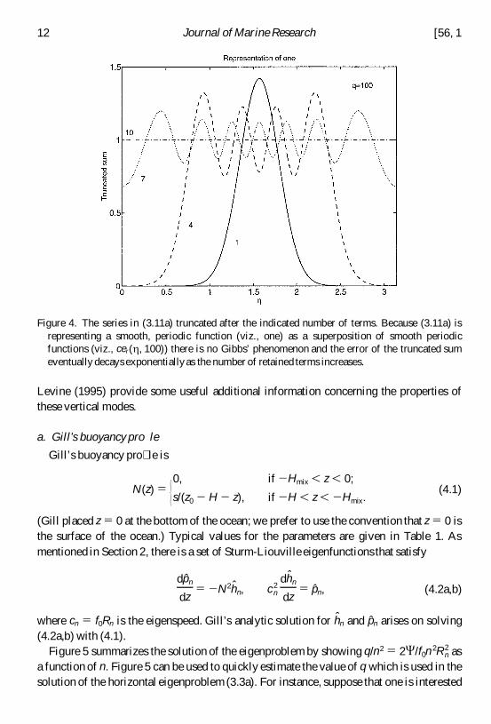
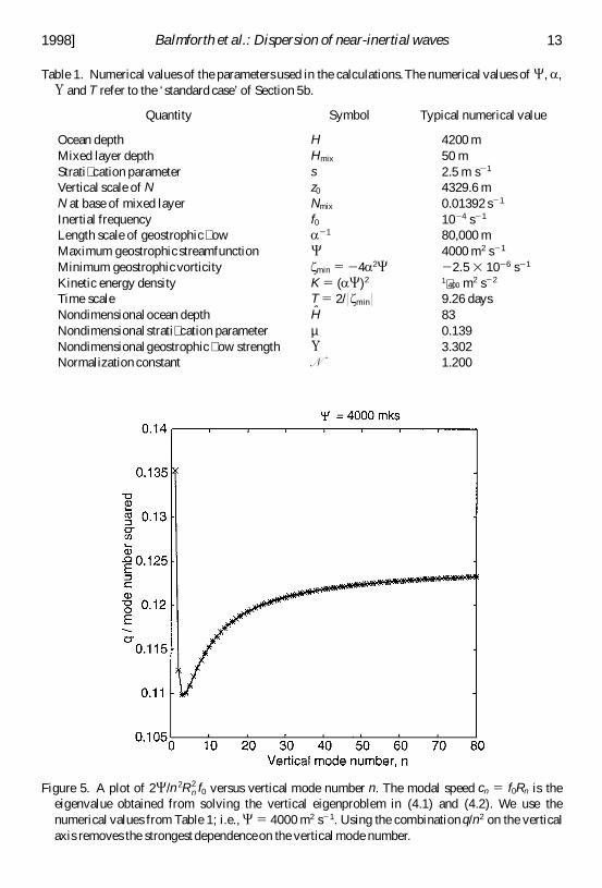
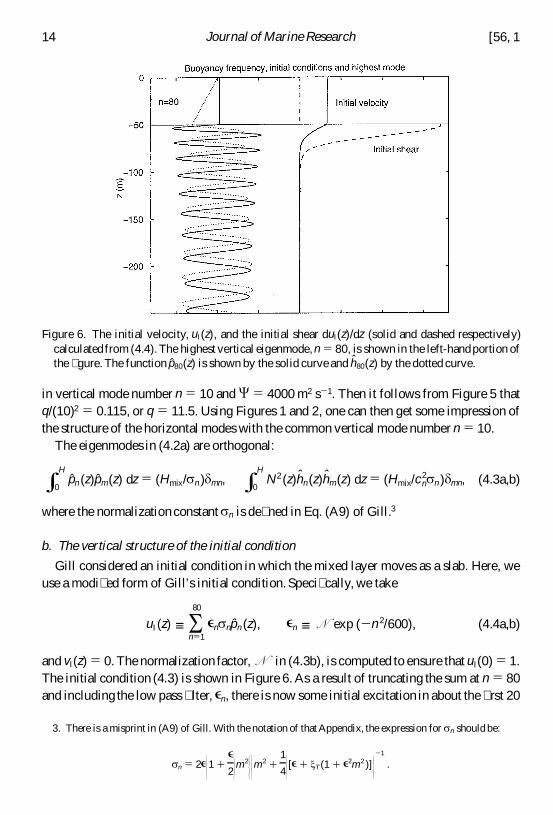
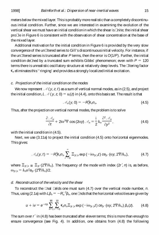
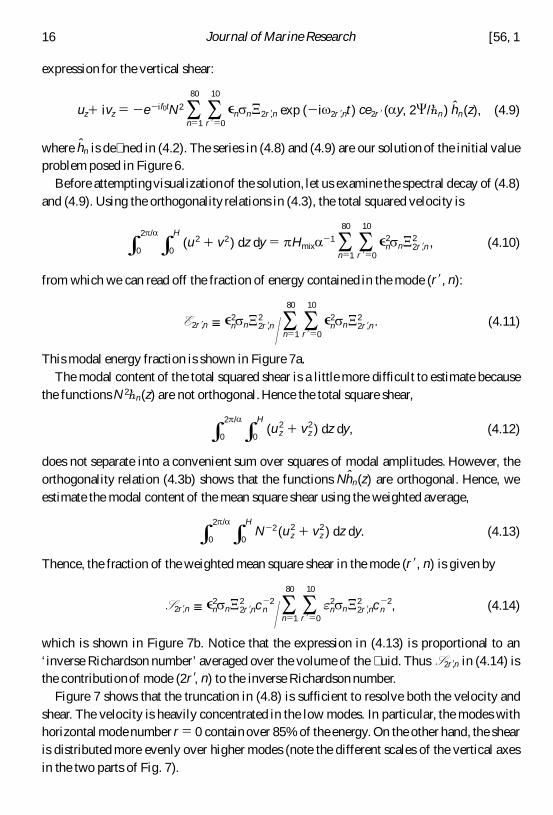
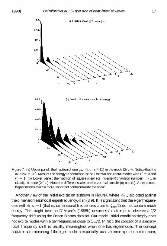
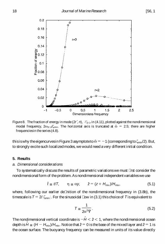
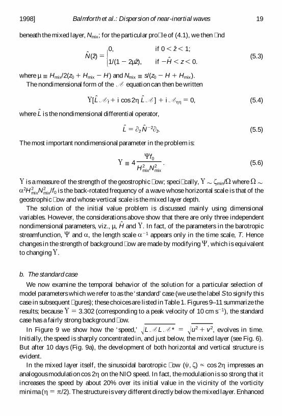
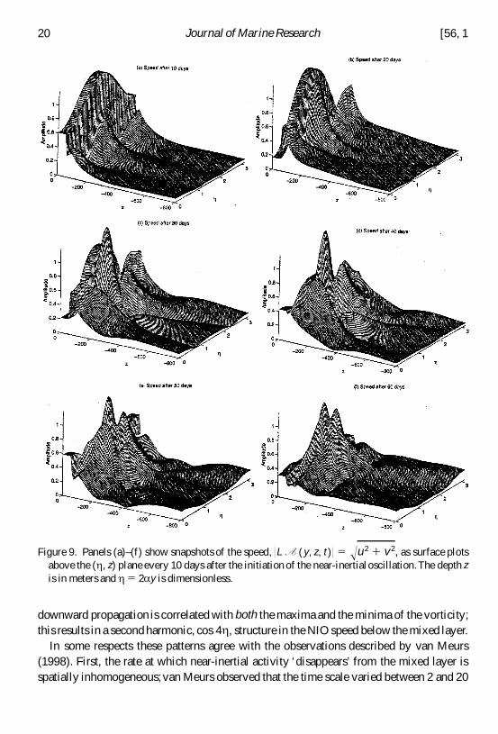
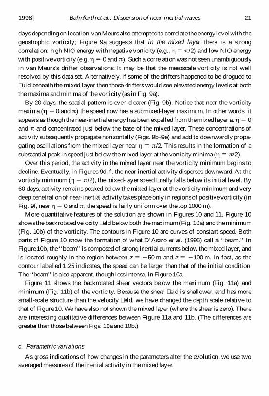
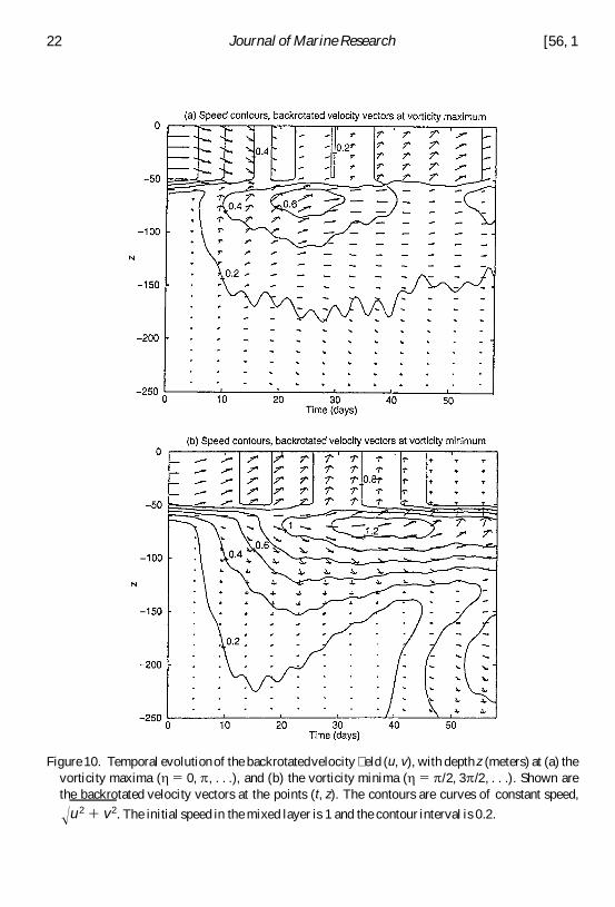
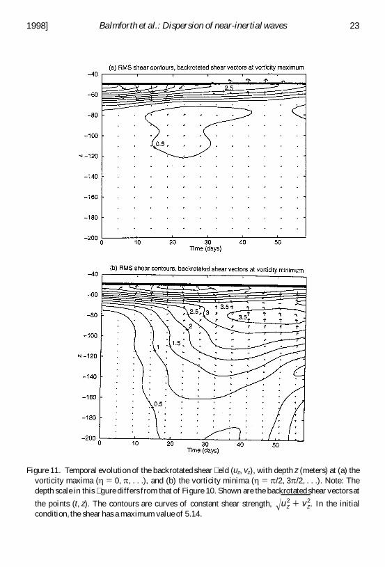
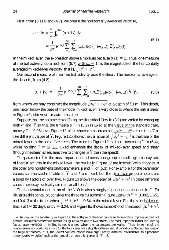
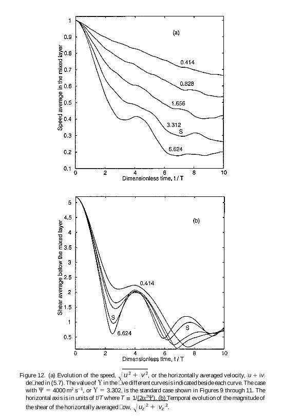
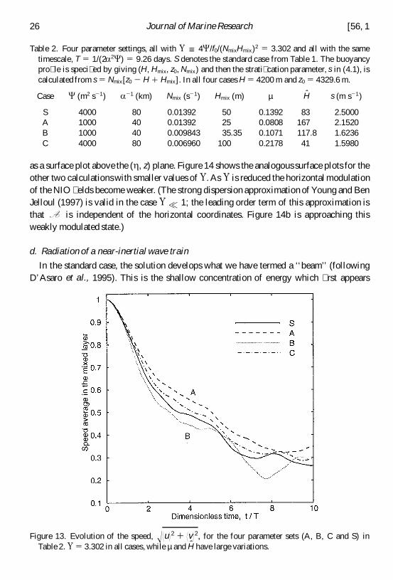
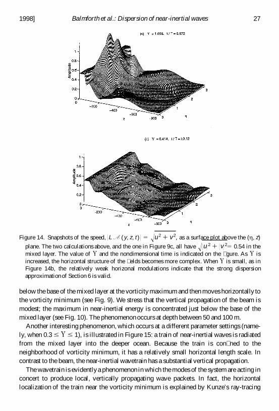
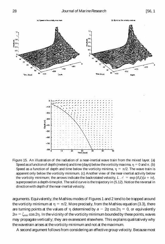
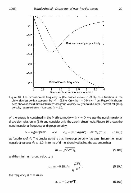
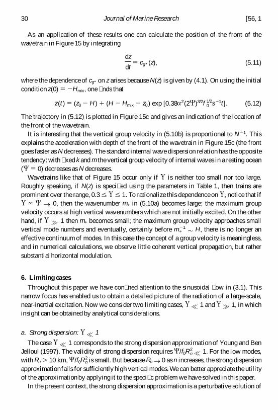
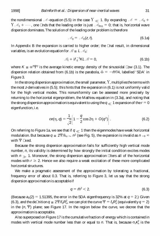
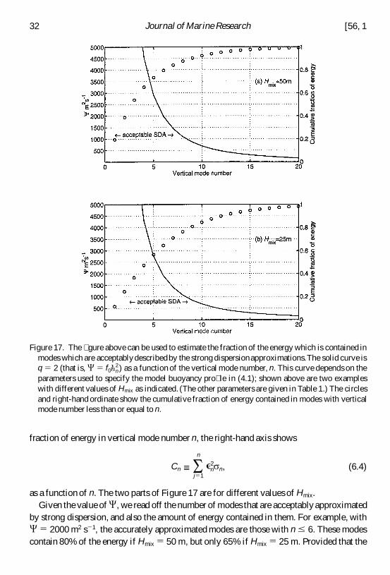
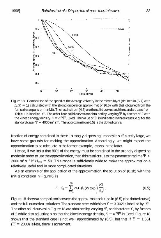
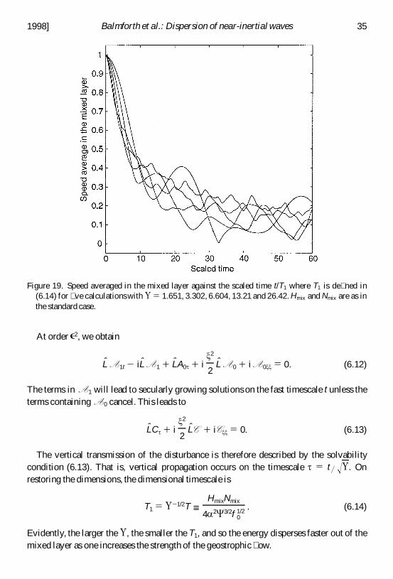
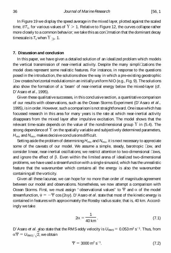