Embed Size (px)
Citation preview

Rowan University Rowan University
Rowan Digital Works Rowan Digital Works
Theses and Dissertations
7-24-2011
Enhanced degradation of fats, oils and greases in domestic Enhanced degradation of fats, oils and greases in domestic
wastewater sewer networks and grease interception systems wastewater sewer networks and grease interception systems
using peat humic substances using peat humic substances
Matthew Hunnemeder
Follow this and additional works at: https://rdw.rowan.edu/etd
Part of the Chemical Engineering Commons
Recommended Citation Recommended Citation Hunnemeder, Matthew, "Enhanced degradation of fats, oils and greases in domestic wastewater sewer networks and grease interception systems using peat humic substances" (2011). Theses and Dissertations. 41. https://rdw.rowan.edu/etd/41
This Thesis is brought to you for free and open access by Rowan Digital Works. It has been accepted for inclusion in Theses and Dissertations by an authorized administrator of Rowan Digital Works. For more information, please contact [email protected].

ENHANCED DEGRADATION OF FATS, OILS AND GREASES IN DOMESTIC WASTEWATER SEWER NETWORKS AND GREASE INTERCEPTION
SYSTEMS USING PEAT HUMIC SUBSTANCES
by Matthew Gregory Hunnemeder
A Thesis
Submitted to the Department of Chemical Engineering
College of Engineering In partial fulfillment of the requirement
For the degree of Master of Science
at Rowan University
April 27, 2011
Thesis Chair: Zenaida Otero Gephardt, Ph.D., P.E.

© 2011 Matthew Gregory Hunnemeder

iii
Acknowledgements
The author gratefully acknowledges the support of JSH International and Rowan
University. The author expresses the utmost appreciation and gratitude to his research
advisor, Dr. Zenaida Otero Gephardt, and the University Committee Members, Drs.
Dianne Dorland, Gregory Hecht, Robert Hesketh, and Kauser Jahan. The author also
gratefully acknowledges the assistance from the Rowan University Department of
Chemical Engineering staff, Ms. Susan Patterson and Mr. Marvin Harris, and
undergraduate engineering clinic team members, John Burke, Stephen Clarke, Amy
Manaresi, and Theodora Maravegias. Finally, the author gratefully acknowledges the
assistance and support of his parents, Gregory and Robin Hunnemeder.

iv
Abstract
Matthew Gregory Hunnemeder ENHANCED DEGRADATION OF FATS, OILS AND GREASES IN DOMESTIC
WASTEWATER SEWER NETWORKS AND GREASE INTERCEPTION SYSTEMS USING PEAT HUMIC SUBSTANCES
2009/10 Zenaida Otero Gephardt, Ph.D., P.E.
Master of Science in Chemical Engineering
The efficacy of peat humic substances in enhancing the degradation of fats, oils
and greases (FOG) was investigated under controlled laboratory conditions using bench
scale well-mixed bioreactors. An experimental design was used to evaluate the effects of
temperature and peat humic substance (PHS) concentration on FOG degradation in
domestic wastewater for a temperature range from 10°C to 30°C and a PHS concentration
range from 0 to 20 ppm(v). Factors and interactions significantly affecting the rate of
FOG degradation were identified, and models to predict FOG degradation rates as a
function of PHS concentration and temperature were developed. The models were used to
develop a PHS dosage calculation technique for field operations. Results indicate that
PHS can enhance FOG degradation rates by up to a factor of 2, and microbial cell growth
rates by up to a factor of 3. Atmospheric hydrogen sulfide generation increased with high
PHS concentration at high temperature. The rate of FOG degradation using grease
interceptor material was studied at 25°C and a PHS concentration of 500 ppm(v). In these
systems, PHS was observed to increase the rate of FOG degradation by up to a factor of
2, and microbial colony growth rates by up to a factor of 5. This work indicates that PHS
can enhance FOG degradation rates and increase microbial growth rates in wastewater
treatment systems. These results have significant implications for wastewater treatment
applications.

v
Table of Contents
Abstract iv
List of Figures vii
List of Tables viii
Chapter Page
Chapter 1: Introduction 1
1.1 Purpose of Experiment 2
Chapter 2: Literature Review 3
2.1 Wastewater Components 3
2.2 Wastewater Treatment Process Conditions 6
2.3 Microbial Activity 8
2.4 Wastewater Facilities 11
2.5 Sewer Design 12
2.6 Wastewater Treatment 14
2.7 Humic Substance 17
Chapter 3: Materials and Methods 20
3.1 Peat Humic Substance 20
3.2 Bioreactor Experiments 20
3.3 Statistical Methods and Analysis 34
Chapter 4: Results 37
4.1 Domestic Wastewater Study 37
4.2 Grease Interceptor Material Experiment 46
Chapter 5: Discussion 49
5.1 Domestic Wastewater Study 49

vi
Table of Contents (Continued)
5.2 Grease Interceptor Material Experiment 54
5.3 Experimental Limitations 55
Chapter 6: Conclusions & Recommendations 57
References 59
Appendices 63
Appendix A: Experimental Data 64
Appendix B: Calibration Data 73
Appendix C: Other Experiments 76

vii
List of Figures
Figure Page
Figure 1 Benchtop Bioreactor System Inside Fume Hood 22
Figure 2 Sample Prepared for FOG Quantification 24
Figure 3 MTUD Pumping Station #917 28
Figure 4 Experimental Design Matrix 29
Figure 5 H2Satm Sample Draw Detection Scheme 31
Figure 6 Heterogeneous Restaurant Grease interceptor Material 32
Figure 7 July Wastewater Sample FOG Degradation 38
Figure 8 Pareto Variable Significance Charts 40
Figure 9 Empirical Response Surface Analysis Models 42
Figure 10 January Wastewater Sample Bioreactor pH 43
Figure 11 July Wastewater Sample H2Saq Concentration 44
Figure 12 July Wastewater Sample H2Satm Concentration 45
Figure 13 Bioreactor Equivalency Experiment 46
Figure 14 Grease Interceptor Experiments 9 & 10 47
Figure 15 FOG Calibration 74
Figure 16 H2Saq Calibration 75
Figure 17 Sterile Oil-Water – Non-sterile PHS Experiment Results 76
Figure 18 Preliminary Wastewater Experiment Results 77
Figure 19 Batch Jar Experiment Results 80

viii
List of Tables
Table Page
Table 1 Experimental Conditions Coded for Design 36
Table 2 Experimental Design Results 38
Table 3 Degradation Model Regression Coefficients 41
Table 4 Dissolved Oxygen Results 42
Table 5 July Wastewater Sample Microorganism Counts 45
Table 6 Grease Interceptor FOG Degradation Results 47
Table 7 Grease Interceptor Microorganism Counts 48
Table 8 January Sample Wastewater FOG Data 64
Table 9 July Sample Wastewater FOG Data 65
Table 10 July Sample Wastewater H2Saq and H2Satm Data 66
Table 11 Grease Interceptor Material FOG Data 67
Table 12 January Sample Wastewater pH 68
Table 13 July Sample Wastewater Microbial Quantification Data 69
Table 14 July Sample Wastewater Microbial Quantification Data Summary 70
Table 15 Grease Interceptor Material Microbial Quantification Data 71
Table 16 Grease Interceptor Material Microbial Quantification Data Summary 72
Table 17 FOG Concentration Calibration Data 73
Table 18 H2Saq Concentration Calibration Data 75
Table 19 Sterile Oil-Water – Non-sterile PHS Experiment Data 76
Table 20 Preliminary Wastewater Experiment Data 77
Table 21 Non-biological H2Saq Concentration Experiment Data 83

1
Chapter 1: Introduction
Human population growth has led to increases in liquid and solid wastes as well
as air emissions. Wastewater, a combination of liquid or water-carried wastes is removed
from all varieties of establishments including residences, institutions, commercial and
industrial operations. Untreated wastewater contains nutrients and numerous pathogenic
microorganisms which may stimulate the growth of aquatic flora. Where untreated
wastewater collects and accumulates, the decomposition of the organic matter it contains
can lead to nuisance conditions including the production of malodorous gases. The
removal of wastewater from its sources of generation and its subsequent treatment or
reuse is necessary to sustain public health and the environment [1], [2].
Increases in legislated regulations regarding wastewater effluents have been a
result of high concentrations of biodegradable organic pollutants [3]. Due to the severe
consequences associated with the release of pollutants, particularly fats, oils and grease
(FOG), the U.S. Environmental Protection Agency, states, and cities regulate the
discharge of oil and grease into sanitary sewer collection and treatment systems [4]. FOG
is generated everyday by residential sewer usage and commercial establishments. Federal
regulations require municipal utility and sewer collection entities to properly manage,
operate, and maintain the collection system. The primary means of controlling FOG
blockages is to capture and retain FOG materials before discharge into sewer systems
through the use of passive interception devices [4].
1.1 Purpose of Experiment
This study examines the potential of peat humic substances as an additive for
aiding the remediation of the wastewater pollutants; fats, oils and greases (FOG) and

2
hydrogen sulfide in sewer networks and grease interceptor systems. Humic substances are
a naturally occurring material and their use in wastewater treatment is especially
attractive due to their low pollution potential and cost-efficiency [5]. The purpose of this
work is to test the efficacy of these substances under controlled laboratory conditions and
determine their effect on FOG degradation.

3
Chapter 2: Literature Review
Water science involving wastewater differs significantly from other water
sciences in terms of particulate matter and degree of microbial activity. Wastewater
consists of polluted water and solid matter that may clog sewers or settle and lead to
undesirable consequences such as sanitary system overflow (SSO), odor nuisance,
increased maintenance and wastewater treatment performance problems [6]. The
consequences may be severe for local governments and may include responsibility for
clearing clogged pipes, regulatory fines, and pollution of local environments [7]. Federal
regulations require municipal utilities and sewer collection entities to properly manage,
operate, and maintain the wastewater collection network. The primary focus of many
capacity management operations maintenance (CMOM) regulations is the prevention of
fats, oils and grease (FOG) (including waxes and paraffins) discharge to the collection
system [4]. FOG has been found to be a source of capacity reduction and reduced
treatment system efficiency.
2.1 Wastewater Components
Constituents in wastewater may come from a variety of sources. Many wastewater
sources are rich in organic matter and biomass, often quantified by the chemical oxygen
demand (COD). The chemical oxygen demand is a measure of water quality that
indicates the mass of oxygen consumed per liter of solution and is the result of the
microbial activity in a combination of phases, particularly the biofilm and sediment. In
these phases, FOG and sulfur containing pollutants account for a substantial part of
oxygen consumption and are associated with many of the common problems of sewer
networks and treatment facilities [8]. The general problems associated with FOG include

4
reduction in cell-aqueous phase transfer rates, sedimentation, development and flotation
of low-activity sludge, and system clogging. General problems associated with sulfur-
containing pollutants, particularly hydrogen sulfide, include corrosive and toxic
properties, unpleasant odors and the ability to contaminate atmospheres [9].
The sulfur-containing chemical species of importance found in wastewater
include hydrogen sulfide, sulfates, and the sulfur contained in organic material. Domestic
wastewater normally contains these components in varying concentrations depending on
the source and hardness of the wastewater [10]. Domestic sewage normally contains
3 to 6 mg L-1 of sulfur-containing organic material, present mainly as proteinaceous
matter, and also in the form of sulfonates derived from household detergents. Hydrogen
sulfide and other malodorous sulfur compounds are formed from the reduction of these
sulfur-containing organic materials [11]. Atmospheric hydrogen sulfide can be
considered the principal source of many of the problems associated with these species in
wastewater. Hydrogen sulfide, H2S, is a weak diprotic acid that chemically dissociates to
the species HS- and S2-. The proportion of these species is primarily a function of pH and
to a lesser extent, temperature and ionic strength. Hydrogen sulfide crosses the aqueous-
atmospheric phase boundary as a function of process conditions [10]. This results in
maintenance hazards and environmental nuisances for municipalities. Hydrogen sulfide
may also be oxidized from the sewer atmosphere by microbial activity to form sulfuric
acid (H2SO4) which subsequently attacks surfaces and other parts of wastewater facilities
(pumping stations, manholes, reservoirs, etc.) [11]. Microbial activity involving sulfide
generation (sulfate reduction) also has a direct influence to the content of organic matter
measured as COD [10].

5
A significant fraction of the COD from municipal wastewaters is composed of
fats, oils and grease. The FOG fraction of COD is composed of a variety of different
molecules that represent a degree of biodegradability lower than other wastewater COD
fractions such as proteins and carbohydrates [12]. The accumulation of pollutants with
low biodegradability leads to several problems impacting wastewater treatment systems
including: non-optimal operational performance (clogging, fouling, reduction of
separation efficiency), non-optimal microbial activity, and operational nuisance
(increased maintenance, cost and foul odors) [9].
High FOG accumulation in treatment systems, particularly pumping and aeration
systems, may promote the concentration of filamentous microorganisms. High
concentrations of these organisms may cause undesirable pollutant characteristics and
treatment difficulties such as the formation of scum and stable viscous foams at pumping
stations and sewage treatment works [9], [13]. Scum and foams also hinder biomass
flocculation, sedimentation and generate unpleasant odors. FOG is also capable of
forming lipid coats on the biological floc in wastewater. Lipid coating resistance reduces
biological-aqueous phase transfer rates, inhibiting natural biological degradation.
Hydrolysis of FOG produces long-chain fatty acids which are also reported to inhibit the
activity of various microorganisms [9], [14].
From wastewater sources such as domestic and commercial kitchens, a significant
portion of FOG is made up of fats and oils, also known as lipids. Lipids are a family of
naturally occurring organic compounds that are relatively insoluble in water. Lipids
consist of fatty acid molecules chemically bonded with glycerol by ester linkages and are
biologically assembled by dehydration reactions and disassembled by hydrolytic

6
reactions [15]. A simple lipid consists of three fatty acid molecules bonded to the three-
carbon molecule, glycerol, and is also known as a triglyceride. The accumulation of fatty
acids is a source of microbial inhibition [14]. Fatty acids consist of long hydrocarbon
chains (attributing hydrophobic properties), with a carboxyl group at one end, varying in
chain length and degree of saturation [15]. Generally, carbon chains consisting of 16 to
18 carbon atoms in length are designated as long-chain fatty acids (LCFA), commonly
found in edible fats and oils [13]. The component fatty acids in domestic and commercial
wastewater source edible fats and oils vary considerably. Most land-animal lipids contain
saturated LCFA and most plant and fish lipids contain unsaturated fatty acids [16].
Lipids are essential components of all cells. Biologically, the major functions of
lipids are cellular structure and energy storage. The fatty acid composition of cells varies
between species and within species due to temperature (growth at low temperatures
favors shorter-length fatty acids, higher temperatures longer length fatty acids). Fatty
acids are good electron donors for microorganisms [16]. Energy from fatty acids are
oxidized by a process called beta oxidation. The products of this process may be acetate,
carbon dioxide, and methane depending on the microbial species involved. A significant
amount of microorganism families capable of metabolizing lipids in wastewater
environments are presently known and many are yet to be discovered.
2.2 Wastewater Treatment Process Conditions
Dissolved oxygen, pH and oxidation-reduction potential (ORP) are characteristics
of wastewater which are central to biological wastewater pollutant transformation. They
may fluctuate as a function of sewer microbial activity and wastewater source. The pH of
many commercial wastewater sources is often basic due to the presence of equipment

7
cleaning solutions and degreasers [4]. Wastewater pH subsequently decreases upon
entering the collection system due to microbial activity including the fermentation of
FOG (production of acetic acid), oxidation of hydrogen sulfide and the formation of
volatile acids under anaerobic conditions [10]. Decreasing pH is often observed in sewer
networks as a function of relatively high wastewater residence time, high COD and
temperature in pipes. The oxidation-reduction potential, in which dissolved oxygen (as an
electron acceptor) is pivotally important, governs the mode of microbial transformations
in sewer wastewater. The ORP is the difference in electric potential measured between a
platinum electrode and a hydrogen standard electrode. In an aqueous medium, the ORP is
an approximate measure of the equilibrium existing between the reducing and oxidizing
substances in water. Generally, positive values of ORP correspond to oxidizing
conditions - negative values correspond to reducing conditions [10], [11]. Dissolved
oxygen influences both the pH and ORP and is a determining factor for microbial
respiration. The dissolved oxygen concentration in wastewater is a function of the initial
oxygen concentration, oxygen consumption rate, and bulk water reaeration. Sewer
networks are designed to allow for reaeration of wastewater yet dissolved oxygen
concentrations are subject to large fluctuations [17].
Temperature is one characteristic of wastewater that has a significant impact on
pollutants as applied to wastewater collection systems. Biological activity including the
utilization of FOG and reduction of sulfates takes place at a range of temperatures in
collection systems which are responsible for the selection of dominant species. There are
two main classes of microorganisms considered in biological remediation of FOG in
wastewater: mesophilic and thermophilic. Temperatures that provide optimal growth for

8
mesophilic organisms range from 20°C to 45°C and range from 45°C to 80°C for
thermophilic organisms [18]. Thermophilic temperatures are typically seen in digesters
treating wastewater with a defined composition and high fat content such as those found
in the dairy or meat processing industries [9]. Commercial grease interceptors have also
been known to experience temperatures close to the thermophilic range [4]. Mesophilic
temperatures are found in most parts of a sewer network. However, psychrophilic
organisms also exist in sewer networks, exhibiting optimal growth at temperatures which
do not exceed a maximum of 20°C. Some microorganisms found in sewer systems can
grow over a wide range of temperatures; for example: E. coli has the ability to grow over
a temperature range of 8°C to 48°C with optimal growth occurring at 39°C [18].
However, generally only mesophilic and psychrophilic microorganisms play a major role
in biological in-sewer processes.
2.3 Microbial Activity
Microbial respiration in sewage systems is a function of the concentration of
dissolved oxygen in the bulk liquid and by wastewater component and are referred to as
aerobic, anoxic and anaerobic. During aerobic conditions (oxygen > 0.5 mg/L)
microorganisms may utilize oxygen as a terminal electron acceptor (TEA) for metabolic
respiration. When the oxygen in the bulk liquid has been depleted, anoxic modes of
metabolism occur to continue to provide the microorganisms with energy. Anoxic
respiration utilizes TEAs which are less thermodynamically favorable for microbial
respiration (compared with oxygen) such as nitrate. Addition of nitrate to promote anoxic
processes (denitrification) is a well-studied method for avoiding anaerobic conditions
[17]. Anaerobic (oxygen < 0.5 mg/L) conditions lead to many of the problems associated

9
with wastewater collection systems. Microorganisms capable of anaerobic respiration
rely on metabolic pathways which produce smaller energy gains when compared with
pathways utilizing oxygen as a TEA [18]. Sulfate has been reported as a common TEA
for anaerobic microbial activity [10]. For example, acetate may be mineralized through
the three aforementioned processes as expressed by the following stoichiometric
equations:
Aerobic respiration: CH3COOH + 2O2 → H2O + CO2 + HCO3–
Anoxic respiration: 5CH3COOH + 8NO3– →4N2 + 10CO2 + 6H2O + 8OH–
Anaerobic respiration: CH3COOH + SO42– → S2– + H2O + CO2 +HCO3
–
Aerobic transformations of pollutants are characterized by high heterotrophic
biomass activity including excelled growth of the biofilm and suspended phases and
corresponding organic substrate hydrolysis, degradation, and consumption. Aerobic
wastewater quality changes include reduced biodegradability and increased compatibility
with mechanical treatments. The magnitude of aerobic transformation varies significantly
depending on initial wastewater quality and sewer system conditions. Using oxygen as a
TEA, organic carbon can be completely mineralized to carbon dioxide by a single
microorganism [19]. Studies have shown that the rate of uptake of dissolved oxygen by
microorganisms present in domestic sewage varies from about 2 mg/L at 15°C and may
increase to values about 20 mg/L as the sewage ‘ages’ within the sewerage system under
aerobic conditions. The average is approximately 14 mg/L h at 15°C [16].
Aerobic FOG metabolism by microorganisms has been documented by several
researchers [13]. The initial attack on triglycerides by microorganisms is extracellular and
involves the hydrolysis of the ester bonds by lipolytic, hydrolytic enzymes (lipases)
which remove the fatty acids from the glycerol molecules [9]. Once hydrolyzed, fatty

10
acids may enter a microbial cell and either catabolized directly or incorporated into
complex lipids. Glycerol is released into the bulk liquid [20]. Lipases have been found by
researchers to be both highly- or non-selective in regards to attacking lipids containing
specific fatty acids. One reason for this difference in fatty acid selectivity has been
suggested to be due to the substrate dependency of a microbial population. The removal
of FOG by different organisms has been investigated in batch-growth studies and results
indicate that removal could be significantly affected by the substrate specificity of the
induced extra-cellular lipases, the physical and chemical characteristics of the substrate,
and the pH of the culture medium [21], [22].
Anaerobic transformations are characterized by hydrolysis and fermentation of
organic substrate, methanogenesis, and sulfate reduction. The rate at which anaerobic
transformations proceed is relatively lower than aerobic transformations [17]. The
consumption of readily biodegradable (fermentable) organic substrate is generally slower
than production of fermentable substrate from hydrolysis. Slight net production of
fermentable substrate may be expected of this mode of transformation [17]. Anaerobic
decomposition (particularly in inundated wetland soils) requires many interdependent
microbial processes (known as syntrophy) and can generate both CO2 and methane as
end products of organic substrate mineralization [20].
Anaerobic transformations in sewer networks are generally associated with
sulfide generation by sulfate reducing bacteria (SRB) [11]. SRB are widespread in
aquatic and terrestrial environments that become anoxic or anaerobic as a result of
microbial decomposition processes. SRB may conduct dissimilatory reduction (producing
an inorganic compound from an organic compound). The genera group I (non-acetate

11
oxidizers) of SRB can utilize lactate, pyruvate, ethanol, or certain fatty acids as electron
donors reducing sulfate to sulfide. The genera of group II (acetate oxidizers) specialize in
the oxidation of fatty acids, particularly acetate, reducing sulfate to sulfide. The sulfide
generation rate is a function of several factors including pH, temperature, nutrients,
presence of biofilm on sewer surfaces, presence of sulfate reduction inhibitors, and the
oxidation-reduction potential (ORP). Sulfate is often not the limiting nutrient in sulfide
generation unless its concentration is below 10-15 mg/L [11]. Wastewater components
required for SRB activity include electron-donating organic matter (including FOG) and
sulfate or sulfur-containing organic substrate (TEAs). Wastewater pH has an influence
over sulfide generation, but rates appear to be highest for pH ranges between 6.5 and 8.0,
which is typical of domestic wastewater [11]. A small amount of reduced sulfur is
assimilated by the bacteria, but most is released into the external environment as sulfide
ions [10].
Anaerobic treatment of lipid rich wastewater or solid waste is difficult in practice
due to significant accumulation of LCFA derived from hydrolyzed lipids [17]. Long
chain fatty acids are toxic to anaerobic bacteria and sulfate reducing bacteria [14], [23].
The unionized form of these acids, namely the long chain free fatty acids may decrease
the availability of ATP to many microbial species. However, it has also been
demonstrated that improved microbial fatty acid biodegradation and tolerance can be
achieved by substrate acclimatization [14].
2.4 Wastewater Facilities
Sewer networks collect source wastewater and discharge at wastewater treatment
facilities. Traditional facilities consist of three general types of wastewater treatment

12
processes: the primary and secondary treatments which remove the bulk of pollutants and
tertiary treatment which decreases the concentration of pollutants to meet regulatory
standards before discharge or recycle [5]. Primary treatment (generally physical
processing and/or chemical addition) removes settable solids and secondary treatment
(biological processes) breaks down waste stream pollutants to non-toxic or benign
products. Tertiary treatment, including adsorption on activated carbon, ion exchange and
chemical oxidation may be expensive and affected greatly by the efficacy of the primary
and secondary treatments [5], [24]. In several instances, traditional wastewater treatment
has been found to be too expensive or insufficient in reducing the concentration of
pollutants in wastewater streams [5]. Many industrial and commercial establishments
generate wastewaters for which current treatment technologies remain unacceptable and
unvalidated [24]. Wastewater treatment design has traditionally considered treatment to
start at the “end-of-pipe” which had limited the improvement of treatment processes to
treatment facilities. However, it has been observed that chemical and biological in-sewer
processes affect the sewer itself and subsequent treatment facility performance [17].
Thus, the “sewer as a bioreactor” concept has become corollary to “pipe-and-plant
treatment” allowing for improved engineering, sustainability and treatment performance.
Currently, rather than existing as solely a collector and transporter of wastewater, the
sewer itself may be considered a complex processing system that transforms pollutants
and characteristics of wastewater [17].
2.5 Sewer Design
Design and investment in the understanding of sewer networks has, in general,
mainly focused on the physical aspects of sewer performance (hydrology, hydraulics and

13
solids transport). More recently, significant research advancements have included more
consideration for microbial activity such as reaeration, water velocity and materials of
construction [17], [25]. Low cost, naturally occurring, sustainable and non-polluting
treatment solutions are ideal for enabling increases in organic matter removal efficiency
and promoting high quality effluents [17].
In-sewer wastewater quality transformations generally take place in four phases:
suspended water, sewer sediments, biofilm and sewer atmosphere. Chemical and
biological processes occur in situ in these phases and by the exchange of material across
phase boundaries. Influencing factors include wastewater constituents and microbial
activity which are affected by the sewer design which determines sewer process
conditions. The sewer networks in many municipalities are the result of years of
investment and are continually maintained and revised with pollution control strategies
[17]. Volumetric flow capacity is a main factor in the design of sewer networks
accounting for the daily fluctuation of sewer usage (referred to as time series) and also
fluctuation due to precipitation. This design factor is critical to avoiding septic system
overflow and has a large impact on microbial activity. High water velocity causes
increase in dissolved oxygen concentration and high rates of microbial activity associated
with aerobic respiration. However, high water velocity causes a loss of system biomass in
both aqueous and sediment phases decreasing the overall microbial activity. Conversely,
periods of low water velocity may cause high sedimentation of suspended solids and
microbial activity leading to a high oxygen uptake rate and anaerobic activity. During
these different flow periods chemical components of wastewater may undergo significant
chemical and microbial transformation, especially in warm temperature regions or sewer

14
sections. Due to the high and uncontrolled fluctuation of the time series, both pollutant
concentrations and process conditions may fluctuate heavily [17]. Therefore, biological
wastewater transformation processes proceed under significantly variable system
conditions. In addition, models for the degradation of well-defined chemical
compositions of FOG which allow for more deterministic modeling of biological
processes become less accurate when applied to sewer network systems [25].
In addition to fluctuation in water velocity, sewer networks may be subject to
seasonal temperature variation and stratification depending on the region of interest. It is
reported that in cold weather, the efficiency of the biological processes may decrease and
many of the pollutants of concern, particularly FOG, which solidifies at low temperature,
become resistant to biological degradation [12]. Thermal energy is a significant factor
driving microbial growth and activity. Sewer temperatures may fluctuate by as much as
19°C between the extremes of seasons depending on the geographical location of the
sewer network [26]. Temperature stratification may be a significant factor in pretreatment
systems and in wet wells. Plumes of high temperature water have been hypothesized to
displace pollutants and facilitate their transport through the collection system [4]. Water
networks may also experience temperature stratification also influencing biological
transformations [26].
2.6 Wastewater Treatment
Many industries including food processing and service have experienced an
extensive range of problems related to the treatment of oil- and grease-containing
wastewater prior to sewer discharge. Treatment of this wastewater prior to sewer
discharge and main wastewater treatment processing is required by Federal and local

15
regulations and plays an important role in maintaining wastewater processing efficiency
and pollution control. Unrestrained FOG from industrial pretreatment systems can be a
nuisance to biological treatment systems, especially in conventional mesophilic processes
[2], [27]. A variety of pretreatment systems are employed to remove FOG and prevent
associated problems, however commercially available pretreatments have, in some cases,
been considered to deliver inadequate performance [3], [6]. Many commercially available
systems act primarily as solid separators and operate marginally as biological treatment
processes [27]. The technology of biodegradation as a pretreatment has not yet been fully
exploited in the processing of organic material present in wastewater streams. Operators
of conventional pretreatment systems and biological nutrient supplement systems would
benefit significantly from any commercial development of a product or process that
would improve grease control [4].
A variety of commercial FOG-restraining pretreatment systems are commercially
available such as grease interceptors, tilted plate separators, dissolved air flotation
systems and physical-chemical treatments. The main technique for separating oils and
fats from commercial restaurant and fast-food wastewater is by grease interceptors or
grease collection methods. A grease interceptor is primarily a physical separation unit; a
vessel through which wastewater passes a series of baffles in laminar-flow conditions at a
rate that allows fat/oil particles to rise to the surface before reaching the trap outlet [9].
The separation principle is based on Stoke’s Law relating the rising velocity of a lipid
particle to its radius, and on the theory that the separation efficiency is independent of
depth [9]. In practice, grease interceptors are designed to allow sludge to accumulate at
the bottom of the device and fat to accumulate at the top. However, non-optimized design

16
and sizing of these systems may lead to discharge of FOG pollutants beyond regulatory
standards. Also, grease interceptors tend to become unaesthetic in terms of maintenance
and may cause localized air pollution [9].
Other commercially acceptable techniques take advantages of different physical
properties for improving separation efficiency of FOG. Tilted plate separators provide a
high surface area for separation and are also available as pre-packaged units. However,
the high surface area may be more susceptible to fouling and cleaning of the system is
time-consuming. Dissolved-air flotation systems increase the rate of rise of FOG by
forming micro-bubbles which attach to FOG particles. However, high air-loading rates,
raw wastewater recycling and water temperature are critical parameters to maintain
efficient operation. Chemical-physical treatments reduce organic COD loads in
wastewater by protein and fat precipitation or flotation using chemical compounds such
as aluminum sulfate, ferric chloride, or more commonly, lyme. These compounds are
intended to break fat emulsions and coagulate fat particles, which can then be readily
separated by physical means such as flotation or sedimentation. Use of these
pretreatments is not expected to be widespread due to high cost of chemical reagents and
formation of problematic sludge during flocculation [9].
Significant research advancements have been made toward treatment of defined-
composition industrial wastewater [9]. Food processing industries generating high FOG
content wastewaters may operate bioreactors for biodegradation of waste streams. These
bioreactors may operate in single units or staged in series under a variety of conditions
(anaerobic, aerobic, mesophilic or thermophilic). Many industrially operated bioreactors
include a chemical or enzymatic hydrolysis pretreatment step for the reduction of FOG

17
particle size. FOG particle size regulates the biodegradability and bioavailability of
substrate materials. Alkaline hydrolysis pretreatments have been mostly tested in waste
activated sludge or municipal waste. Treatment with NaOH has been shown to increase
the ratio of soluble substrates and reduce the volatile solid content during anaerobic
digestion. However, increased pH from alkaline pretreatments may have deleterious
effects for subsequent operations and research for alkaline treatments regarding complex
waste from wastewater collection systems is insufficient [9].
Biological enzymes, particularly lipases, have been used in the treatment of
domestic wastewaters and in the cleaning of sewer systems, cesspools, sinkholes, and in
the effluents of restaurants [9]. Several patents exist for the application of hydrolytic
enzymes, including hydrolases and lipases, in wastewater treatment. Pretreatment with
pancreatic lipases has been reported to reduce FOG particle size by 60% although high
doses were required to obtain a substantial reduction in laboratory reactors [27]. Multiple
inoculations of the reactors were found to be necessary for establishing proper conditions
and microbial activity. Hydrolases, biological enzymes produced by fungi, are capable of
degrading the most complex organic compounds. This wide-spectrum degradation of
organic compounds enables a considerable increase in organic matter removal efficiency
in laboratory bioreactors [9].
2.7 Humic Substance
Addition of humic substance is an attractive means for wastewater remediation
due to its natural origin and low pollution potential. It is found among other dissolved
organic matter in the natural environment such as compost heaps, marine and lake
sediments and peat bogs and constitutes about 60-70% of soil organic matter and 30-50%
18
of surface water organic matter on earth [5]. Humic substance is widely reported to
stimulate plants through a mechanism associated with soil microbial activity and binding
of readily absorbed soil contaminants [28]. The concept has been extended to both
aerobic and anaerobic digestion of municipal sewage showing substantially increased
process activity. In a two-year study of anaerobic digestion of municipal waste with peat
humic substance addition, positive observations included an increase conversion of
organics to combustible gas, changes in sludge character, reduction of sludge volume,
and elimination of odors [29]. Other laboratory tests using activated sludge found
aqueous humic substance to have a high affinity for organic material, increasing non-
polar organic compound solubility [30]. Other field experiments have demonstrated the
successful detoxification of a plant-operated activated sludge aerator contaminated with
inhibitory metals [29].
Humic substance is a high-molecular weight polymeric mixture of partially
decayed organic materials derived partly from the constituents of microorganisms that
have resisted decomposition and partly from refractory plant materials [5]. It exists in
both solid and aqueous phases as sub-micron colloids and dissolved anionic
macromolecules, respectively; each phase exhibiting unique chemical properties.
Extracted humic substance from natural environments is a heterogeneous mixture of
molecules containing multiple chemical functional groups. Common chemical (free and
bound) functional groups to both aqueous and solid phases include phenolic groups,
quinone structures, nitrogen and oxygen as bridge units and COOH groups variously
placed on aromatic rings [5]. Aqueous humic substances molecular structure has been
described as containing glassy and rubbery domains: small quantities of high surface area

19
carbonaceous material admixed in a larger amount of solvent-like matter and rigid
structures due to intra-molecular forces and site-specific surface interaction [28].
Observed properties of aqueous-phase humic substance (AHS) are the ability to
create complexes, increase solubility, and facilitate transport of hydrophobic organic
solutes and metals [5], [30]. AHS has been found to have much greater capacity for
creating complexes with organic solutes than the capacity for solid phase humic
substance to absorb organic solutes. It has been reported that the oxygen-containing
functional groups may be largely responsible for regulating properties such as water
solubility, acidity, surface activity, and metal complexing capacity [5]. Humic substance
has been reported to have the ability to accept terminal electrons from some
microorganisms capable of anaerobic oxidation of organic compounds and hydrogen.
This electron transport yields energy to support growth and further enhances the capacity
for microorganisms to reduce other, less accessible electron acceptors due to an electron
shuttling mechanism. These properties suggest that AHS may play a larger role than is
currently understood about the oxidation of organic matter and also about the impact on
the fate of other environmental contaminants [31].

20
Chapter 3: Materials and Methods
The materials, methods and equipment used for all experiments are described
below. All bioreactor experiments were conducted under controlled laboratory conditions
and operated inside a fume hood. An approved job safety analysis was performed before
starting experimentation. All experiments followed standard operating procedures
including a protocol for the safe-disposal of hazardous materials.
3.1 Peat Humic Substance
Concentrated peat humic substance (PHS) was provided by JSH International in
16 ounce HDPE bottles. The same batch of PHS product was used for all experiments.
The PHS is 10% extracted peat humic substance dissolved in water.
3.2 Bioreactor Experiments
Experimental System
Two Eyela® Heavy Duty Benchtop Fermentors (bioreactors), model MBF250
were used for this work. Each bioreactor consisted of a main unit and a fermentation
vessel. The fermentation vessel construction consisted of a 2.5 L borosilicate glass
cylinder with a secondary glass wall and a stainless steel lid. The vessel lid was
constructed with a magnetic drive system for turning an impeller shaft with two impellers
spaced 2.5 in. apart, a four-baffle configuration, and multiple configurable ports. The
secondary glass wall was used as a temperature regulating jacket. A NESLAB™ water
circulator with an operating range of -10°C to 70°C provided uniform temperature
control to both vessels in parallel. Each fermentation vessel docked to a main unit which
controlled agitation speed in a range of 100 RPM to 1200 RPM (for runtimes greater than
24 h) and up to a speed of 1500 RPM (for runtimes less than 24 h). A photograph and

21
schematic of the reactor system with docked bioreactors and temperature control
configuration are shown in Figures 1 a and b. Prior to each experiment, bioreactors were
hand-washed and sterilized in a BetaStar® autoclave at 123°C at 16 psig for 16min. Total
autoclave cycle time was 40 min. Maintenance of rotating parts was performed as
needed.
a) Experimental System

22
Tachometer
Bioreactor
(aqueous)
(atmosphere)
MagneticDrive
NESLAB™Water Circulator
Sam
ple
Line
Main Unit
Laboratory Fume Hood
Gla
ss J
acke
t
b) Schematic of Experimental System
Figures 1 a-b. Bench-top Bioreactor System
Fats, Oils and Greases (FOG) Quantification
The method of FOG quantification used in this work is analogous to United States
EPA Method 1664 [32], [33]. EPA method 1664 Revision A quantifies n-hexane
extractable material (HEM)) from an aqueous matrix. It is a performance-based method
that gravimetrically determines the concentration of hexane extractable material using
laboratory grade n-hexane with 99% purity. The limits of detection for Method 1664 are
5 to 1000 mg/L; extendable by sample dilution [34]. The method used in this work
determines concentration based on infrared (IR) absorption of HEM thin-films extracted
with technical grade n-hexane (98.5% purity). The detection limits of this work are from

23
10 mg/L with accuracy within 10% to an upper detection dependent upon sample dilution
[33].
Sample Extraction & Preparation
Samples were extracted from agitated bioreactors via a liquid sample port. The
liquid sample port line was constructed of a 0.25 in. stainless steel tube inserted through a
liquid sampling port into the fermentation vessel. The line penetrated to a depth between
the two impellers at a radius from the impeller shaft close to the baffles to ensure well-
mixed sampling. The tube-end inside the bioreactor had a 45° edge. The opposite end of
the sample line was connected by silicon rubber tubing to a syringe (5 – 10 ml) outside of
the reactor. The sample line was held in place by a silicon rubber stopper.
The line was cleared of air and debris by passing a minimum of six sample
volumes through the syringe to minimize sample contamination and optimize
reproducibility. A volume of 5 ml was drawn for each sample and transferred into a new
15 ml polypropylene centrifuge tube. Hexane (OmniSolv® Hexanes 98.5%) was added to
each sample for solute extraction and mixed vigorously with a Fisher™ vortexer at 2800
RPM for 45 s. The samples were subsequently centrifuged using a Forma™ centrifuge at
3200 RPM for 3.25 min to ensure well-defined polar (aqueous), non-polar (organic), and
solid layers. Figure 2 shows an example of a sample prepared for quantification.

24
Figure 2. Sample Prepared for FOG Quantification (Grease interceptor material experiment with clearly defined aqueous, organic and solid
phases)
Infrared Absorption (IR)
The Wilks’s InfraCal™ Total Organic Carbon / Total Petroleum Hydrocarbon
analyzer, model HATR-T2, was used to measure the IR absorption of FOG constituents.
The instrument is a compact, fixed-filter, mid-band IR detector with an insignificant
optical air path. The detector uses an attenuated total reflectance (ATR) sample plate
where a prescribed volume of hexane containing extracted material is deposited on a
zirconia crystal window. The hexane and lighter volatiles evaporate, leaving behind a
film that is measured by infrared [32].
The InfraCal™ instrument was operated under a fume hood for safety
consideration and to expedite the evaporation of volatile materials. Prior to making
measurements, the analyzer was switched on and idled for 1 h. HPLC-grade methanol,
hexane and Kimwipes™ were used to clean the zirconia detection window before the
instrument was zeroed. To check for detector malfunction, the absorbance of pure hexane
was tested and compared with known values. From the non-polar extract layer of each

25
sample, 50 µl were deposited on the detector window using a micropipette. Evaporation
of volatile material was allowed for 5 min before measurement of the film. The
absorbance of the HEM film was recorded and converted to FOG concentration using the
calibration curve in Appendix B.
Rate of FOG Degradation
The FOG degradation rate was determined by linear regression of the
concentration measurements as a function of time. The concentration data were readied
for analysis using standard statistical techniques. The first regression point was selected
after the large molecule breakdown phase observed in the majority of experiments. The
last regression point was selected at the naturally occurring end of ingestion period, also
observed in the majority of experiments. The end of the FOG ingestion cycle is identified
by a second large molecule breakdown phase characterized by an increase in FOG
concentration after a general concentration decrease. Each regression contained at least
three data points and allowed for the determination of an average degradation rate
represented by the slope expressed in mg FOG L-1 day-1. This rate is an averaged rate
representative of the complex processes occurring in the bioreactor.
Microbial Quantification
For quantification of viable, colony-forming, microbiological units (CFU) present
at the start and end of the bioreactor trials, a serial dilution method was used. Liquid
assays for colony-forming cell counts from agitated bioreactors were drawn in triplicate
and aseptically preserved in centrifuge tubes with Fisher® BioReagents™ glycerol in a
sample-cryoprotectant ratio of 10:1. The samples were mixed for 10 seconds at 2800
RPM using a Fisher™ vortex mixer and stored in a laboratory freezer at -70°C.

26
Preserved biological assays were removed from storage and thawed for
quantification. Ten Fisher™ micro-centrifuge tubes were prepared for aseptic dilutions.
Each micro-centrifuge tube was filled with 1 mL of nutritionally rich media (Difco™
Lysogeny Broth (LB), Lennox). Dilutions, in a ratio of 1:10, were made by inoculating
the first filled micro-centrifuge tube with 100 µL of the thawed sample and vortex mixing
for 2 s. Dilutions continued in series by transferring 100 µL of inoculated broth from
each previous microfuge tube to the subsequent with mixing until each tube was used.
Each microfuge tube was aseptically plated onto nutritionally rich agar media.
Stackable Fisherbrand™ 100 O.D. x 15 mm petri dishes were prepared with LB and agar,
To each plate, 100 µL of each dilution sample was deposited and distributed over the
plate using a glass rod technique. After an incubation period of 72 h, the plates were
photographed. Plates containing between 30 and 300 individual colonies were selected,
counted and recorded. The sample cell culture density was calculated using Equation 1:
𝜌𝑏𝑟𝑥𝑡𝑟 =
𝐶𝐹𝑈𝑉 ∗ 𝑑𝑓
(1)
where ρbrxtr is the cell culture density of the liquid sample, CFU is the number of counted
colonies, V is the sample volume of dilution (100 µL), and df is the dilution factor. The
cell culture density of the liquid sample calculated as CFU ml-1 were averaged from
triplicate liquid assays to increase the likelihood of accurate representation of the
biological population density inside the bioreactors.
Domestic Wastewater Study
The effects of peat humic substance on the rate of FOG degradation were
investigated in a replicated experimental design. The dissolved oxygen concentration and
system pH were measured for wastewater samples obtained in January 2010; aqueous and

27
atmospheric hydrogen sulfide concentrations were measured for wastewater samples
obtained in July 2010.
Sample Collection
Wastewater grab samples were obtained in the months of January and July from
the Monroe Township Utility Department’s (MTUD) pumping stations #917 (The
Ridings) and #916 (Deschler Farms), respectively. Figure 3 shows pumping station #917
during site research. FOG is visible in an upper left crescent of the well surface. Samples
were obtained on-site. The absence of commercial biological stimulants or oxidizers in
the pumping stations was verified by the MTUD. A bucket-and-chain device with
interchangeable buckets was lowered into the pumping station to obtain samples from the
water surface. A 0.5 gal iron bucket fitted with holes in the bottom and another plastic 5
gal bucket were used for collecting surface FOG and wastewater. The pH and dissolved
oxygen content of the liquid samples were measured on-site using a Hach™ HQ40d
digital meter in conjunction with IntelliCal™ field probes. The liquid and solid samples
were stored together in clean 1 gal. glass containers and transported to the laboratory.
Samples that were not immediately used were stored in laboratory refrigeration at 4°C.
Sample wastewater obtained for preliminary investigation was collected in
October. Sample wastewater obtained for experimental design use was obtained in
January and July. January wastewater samples were used within 18 days and the July
samples were used within 23 days.
28
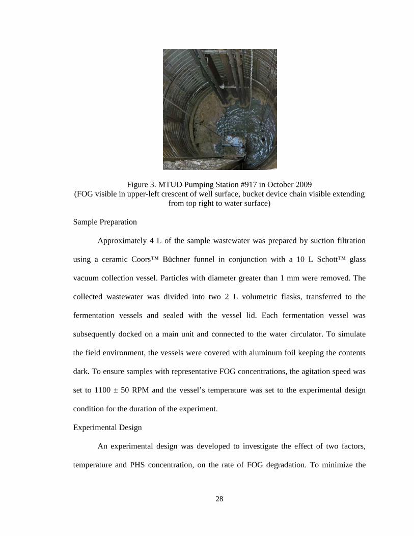
Figure 3. MTUD Pumping Station #917 in October 2009 (FOG visible in upper-left crescent of well surface, bucket device chain visible extending
from top right to water surface)
Sample Preparation
Approximately 4 L of the sample wastewater was prepared by suction filtration
using a ceramic Coors™ Büchner funnel in conjunction with a 10 L Schott™ glass
vacuum collection vessel. Particles with diameter greater than 1 mm were removed. The
collected wastewater was divided into two 2 L volumetric flasks, transferred to the
fermentation vessels and sealed with the vessel lid. Each fermentation vessel was
subsequently docked on a main unit and connected to the water circulator. To simulate
the field environment, the vessels were covered with aluminum foil keeping the contents
dark. To ensure samples with representative FOG concentrations, the agitation speed was
set to 1100 ± 50 RPM and the vessel’s temperature was set to the experimental design
condition for the duration of the experiment.
Experimental Design
An experimental design was developed to investigate the effect of two factors,
temperature and PHS concentration, on the rate of FOG degradation. To minimize the

29
number of required experiments, a 22 factorial design was developed using a PHS
concentration range of 1 to 20 parts per million by volume, ppm(v), and seasonal
wastewater temperatures with a range of 10°C to 30°C (50°F - 86°F) [35]. Factor ranges
were chosen representative of field operating conditions. The design included two center
points at 20°C and 10 ppm(v) PHS to test for system nonlinearity. Figure 4 is a graphic
representation of the design matrix. Tests were performed two experimental points at a
time; each using a similar bacterial sample and the same temperature.
Figure 4. Experimental Design Matrix (Graphical representation)
The experimental design was performed using wastewater obtained from pumping
station site #917 in January. The bioreactors were configured for PHS inoculation, liquid
sampling, venting, pH, ORP measurement, and wastewater sample capacity of 2 L. Once
the bioreactors had reached their specified operating temperature, initial FOG samples
were obtained and the vessels were subsequently inoculated with PHS. For each set of
experiments, FOG concentration, pH and ORP were measured in 24 h intervals from each
bioreactor. For each FOG sample, 1 ml of hexane was used for FOG quantification.
The experimental design was replicated using wastewater obtained from pumping
station site #916 in July due to difficulties in obtaining samples at pumping station #917.

30
The replicate design included the addition of control experiments operated at the design
center point temperature of 20°C. Control reactors used the same microbially active
wastewater samples as the corresponding PHS dosed reactors. PHS concentrations of 0
and 10 ppm(v) were used for the control and design center point, respectively. The
bioreactors were configured for PHS inoculation, liquid sampling, gas sampling, venting
and a sample capacity of 2 L. Initial FOG concentration measurement, PHS inoculation,
and the hexane extraction quantity were replicated identically. For each set of
experiments, FOG concentration, Aqueous and atmospheric hydrogen sulfide
concentration (H2Saq and H2Satm) were measured in 12 h intervals from each bioreactor.
Biological samples were taken before and after each trial for the assessment of colony
forming microorganisms.
Dissolved Oxygen and pH
For continuous measurements of pH, two-channel Thermo™ Orion 720A analog
meters coupled with pH (channel-1) probes were configured for the bioreactors. The pH
probes were calibrated using an internal three point calibration with standards from
Fisher™. Probes were held rigidly in their respective ports using modified rubber
stoppers to maintain them at the correct depth. Dissolved oxygen (DO) and pH were also
measured directly in the unsealed fermentation vessel before and after each experiment
using a Hach™ HQ40d digital meter in conjunction with IntelliCal™ field probes.
Atmospheric and Aqueous Hydrogen Sulfide
To measure the atmospheric hydrogen sulfide concentration (H2Satm), a RKI
Instruments™ GD-K71D H2Satm environmental sample-draw detector was mounted
between the two main units. The sample draw detector had a range of 0-30 ppm(v) and

31
was calibrated using a two point internal calibration with a gas standard from GTS-
Welco®. Atmospheric sampling ports from both fermentation vessels were connected to
a three-way switching valve with rigid laboratory tubing. The switching valve allowed
atmospheric samples to be drawn to the detector, one bioreactor at a time. A dilution
junction was incorporated to further dilute concentrated samples with ambient air. An in-
line moisture and particulate filter was located immediately upstream from the
electrolytic chemical detector. The H2Satm concentration was read directly from the
detection unit. A schematic of the H2Satm detector sample line is shown in Figure 5.
Switching Valve
BioreactorBioreactor
(aqueous)
(atmosphere)
Dilution Valve
Moisture and Particulate Filter
RKI Instruments™ GD-K71D H2Satm
sample draw detectorTo Laboratory Hood Vent
Ambient Air
Figure 5. H2Satm Sample Draw Detection Scheme
The aqueous hydrogen sulfide concentration (H2Saq) measurements were
performed using the extracted wastewater samples for FOG measurement. H2Saq
measurements were performed using a modified method of Cline used for measurement
of sulfide in environmental samples [36]. Prepared diamine reagent was contained in a

32
graduated 100 ml buret. To each bioreactor sample, 1 ml of prepared diamine reagent was
dispensed into the centrifuge tube. The sample was prepared for FOG analysis. After
centrifugation, 3 ml of the aqueous phase was transferred into a cuvette with a
micropipette and stored for 20 minutes to allow color development. The absorbance at a
wavelength of 670 nm was measured using a Milton Roy™ Spectronic 21D and
recorded. Liquid sulfide calibration data are listed in Appendix B.
Grease Interceptor Material Experiment
Grease interceptor material experiments evaluated the rate of FOG degradation
with grease collector material as the main substrate. Experiments were performed at 25°C
(77°F), with 5% (volume) grease in tap water. Typically, 16 ounces of PHS are poured in
the grease interceptor every 24 hours. Based on an industrial grease interceptor with a
liquid holding capacity of 35 gal, the average PHS concentration in the grease interceptor
was approximately 500 ppm(v) h-1. Side-by-side experiments were performed with a
control and a PHS-dosed bioreactor. Two separate batches of grease samples were used
over the duration of these trials. Bioreactors were configured for PHS inoculation, liquid
sampling, and venting. FOG concentration was measured in 12 h intervals and biological
samples were taken before and after each trial for each bioreactor. Due to the high
quantity of extractable content contained in each bioreactor liquid sample, a dilution step
was required before IR measurement. To each bioreactor FOG sample, 5 ml of hexane
were added, and prepared for quantification. From the prepared sample, 1 mL of the
organic layer was diluted in 10 ml of pure hexane and vortexed 5 s to ensure well mixed
samples.

33
Sample Grease Material
Grease collector sample material was provided by JSH International. Samples
contained FOG removed from a restaurant grease interceptor. Samples were collected
from the grease interceptor before business hours of operation and stored in mason jars.
Samples were transported to the Rowan University laboratory and stored in a 4°C
refrigerator if not used immediately.
Sample Preparation
Grease samples were heterogeneous in color and consistency when received.
Figure 6 shows typical grease interceptor material from a restaurant.
Figure 6. Heterogeneous Restaurant Grease Interceptor Material (Collected 6:00am, April 20, 2010)
Samples were warmed in a scientific oven in a temperature range of 30°C and
37°C for at least 3 h to obtain uniformity and increase material flow-ability. A single
main unit was fit with a custom mixing device for mason jar attachment. To prevent
overflow during the mixing process, the volume of material in the sample containers was

34
checked and adjusted. After warming, samples were subsequently docked to the mixing
unit, sealed, and blended to a satisfactory uniform consistency.
The grease sample was prepared in a 5% (volume) system by first preheating to
30°C to improve flowing characteristics. Fermentation vessels were loaded with 100 ml
of grease measured with graduated cylinders. Tap water (1900 ml) was measured with
volumetric flasks and added to the bioreactor. The bioreactors were subsequently sealed
and docked on a main unit. Water circulation lines were connected and the bioreactors
covered with aluminum foil. Agitation speeds were set to a nominal 1100 RPM.
3.3 Statistical Methods and Analysis
Statistical methods were employed depending on the quantity of data. FOG
concentration data were analyzed for the rate of FOG degradation.
Data Preparation
For each FOG concentration measurement, a set of three samples was drawn and
the absorbance of the HEM film for each sample was recorded. An average absorbance
from each set of data was computed for conversion to FOG concentration. A modified
nearest-neighbor method of outlier detection was used in data analysis. The average and
standard deviation of the data set were calculated from the data selected. The two-tailed
student’s t distribution for 95% confidence was compared to the standard calculated t for
the selected value [35]. The average absorbance was then converted to FOG
concentration using the calibration curve in Appendix B. The calibration used was based
on a mixture of olive and rapeseed oil and modeled by a linear, forced-zero trend with an
R2 value of 0.976.

35
Experimental Design
The experimental design and the replicate used biological samples from January
and July. Due to the variation in sewer network conditions and the geographical variation
between biological samples, it was hypothesized that the biological consortium from each
biological sample could be different. Therefore, the design was analyzed for each season
and also with all data combined. The January design was completed without control and
center-point side-by-side replicates; therefore, calculated data were used to complete the
analysis. A ratio of design center points from the January data and July data was
calculated. Two July design control points and one center point were multiplied by this
ratio to calculate three January wastewater sample rates 263, 243, and 196 mg FOG L-1
day -1 found in Table 2.
The response surface method of analysis was selected for application to the 22
factorial designs with center points and controls. The response surface method is used for
modeling and optimization of systems, in which, a response of interest is influenced by
several variables. The form of the relationship between the rate of FOG degradation and
the variables, temperature and PHS concentration, is unknown. However, the response
surface method serves to find a suitable approximation for the true relationship.33 Strong
variable interaction and nonlinearity were hypothesized for this experiment; therefore, the
analysis used second-order polynomial models. Statgraphics Centurion™ v16.1 was used
in the construction and analysis of the experimental design. The design was coded for the
experimental conditions as shown in Table 1 for the response surface analysis.
36
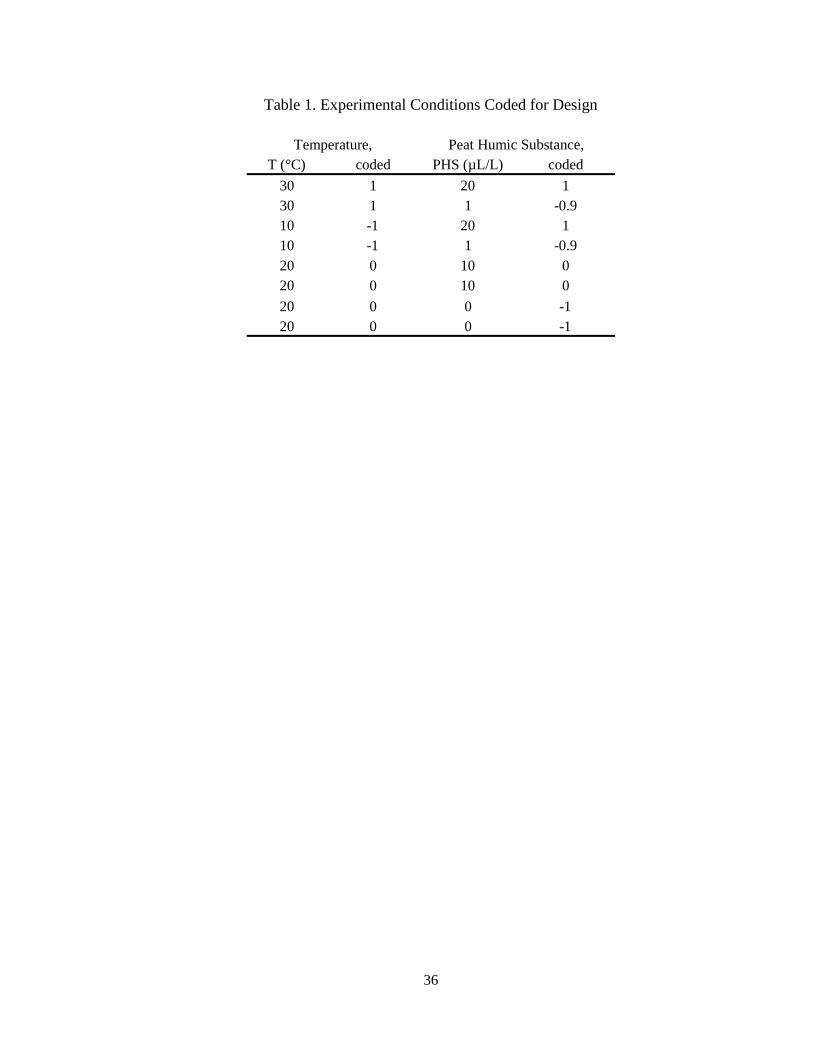
Table 1. Experimental Conditions Coded for Design
T (°C) coded PHS (µL/L) coded 30 1 20 1 30 1 1 -0.9 10 -1 20 1 10 -1 1 -0.9 20 0 10 0 20 0 10 0 20 0 0 -1 20 0 0 -1
Temperature, Peat Humic Substance,

37
Chapter 4: Results
The full composition of experiments and raw data are presented in Appendix A.
FOG degradation rates and cell counts were obtained using the methods described in the
Materials and Methods: Rate of FOG Degradation and Cell Counts sections.
4.1 Domestic Wastewater Study
A replicated 22 experimental design was completed for wastewater studies with
wastewater samples from January and July. The effects of temperature and PHS
concentration on the rate of FOG degradation were studied. Viable colony-forming cells,
pH, DO, and atmospheric and aqueous phase hydrogen sulfide concentration were also
measured in some experiments. January wastewater sample experiments were conducted
over a period of 18 days with each experiment’s duration ranging from 112 to 122 hours.
July wastewater sample experiments were conducted over a period of 23 days with each
experiment’s duration ranging from 82 to 84 hours.
FOG Degradation Analysis
Figure 7 is a plot of FOG concentration as a function of time for a typical
wastewater experiment. As the figure indicates, there is an increase in FOG concentration
at the start of the experiment. The FOG concentration subsequently decreases and, at
approximately 3.5 days, ceases to significantly decrease. This characteristic was observed
in the majority of the FOG degradation results.

38
Figure 7. July Wastewater Sample FOG Degradation (T = 30°C, PHS = 20 ppm(v))
A summary of the experimental design results is presented in Table 2. The rates
obtained for the July and January wastewater samples ranged from 113 to 721 and 25 to
590 mg FOG L-1 day-1, respectively. The highest observed rate of FOG degradation was
721 mg FOG L-1 day-1, which corresponds to a PHS concentration of 20 ppm(v) at a
temperature of 30°C from the July wastewater sample.
Table 2. Experimental Design Results
Standard analysis of variance and experimental design analyses were carried out.
The data were analyzed independently for each (January and July) wastewater sample
and as a combined data set. January and July data analyses were performed at the 90%
0
1000
2000
3000
4000
5000
6000
0.0 1.0 2.0 3.0 4.0
FOG
Con
cent
ratio
n[m
g FO
G L
-1]
Time [days]
Temperature PHS January JulyT (°C) ppm(v) (µL/L) mg FOG L-1 d-1 mg FOG L-1 d-1
30 20 590 72130 1 327 63610 20 42 14810 1 25 11320 10 294 31120 10 243 25720 0 263 27820 0 196 207
Experimental Condition, FOG degradation rate,

39
confidence level to be consistent with the 11% deviation observed in FOG concentration
measurements and the combined data were analyzed at the 85% confidence level (α =
0.15). Figures 2 a-c are Pareto charts for the January, July and combined wastewater data
showing the factors that significantly affect the rate of FOG degradation.
a) January Wastewater Sample
b) July Wastewater Sample

40
c) Combined Data
Figures 8 a-c. Pareto Variable Significance Charts
The pareto charts identify the significance of the variables studied. Bars which
surpass the minimum significant value (vertical line) indicate significance at the specified
confidence level. Both water temperature and PHS concentration have a significant
effect on the rate of FOG degradation in each analysis, with water temperature being
more significant. It is noteworthy that the interaction between water temperature and
PHS concentration (C x T) is significant in the January sample and the second order
temperature effect is significant in the July sample.
Empirical models were developed for FOG degradation rate as a function of PHS
concentration and water temperature. The form of the model is displayed in Equation 2:
RFOG = A + B*[T] + C*[PHS] + D*[T] 2 + E*[T]*[PHS] + F*[PHS] 2 (2)
where RFOG = FOG degradation rate, T = temperature (°C), [PHS] = PHS concentration
(ppm(v)), and A-F are model coefficients. The model coefficients and R2 values for each
analysis are summarized in Table 3.

41
Table 3. Degradation Model Regression Coefficients
Figures 9 a-c display the model-predicted FOG degradation rate as a function of PHS
concentration for the temperatures investigated for each data set.
a) January Wastewater Sample
b) July Wastewater Sample
Data R2 A B C D E FJanuary 0.92 -130.30 15.63 -12.20 0.04 0.65 0.32
July 0.92 386.54 -46.67 2.42 1.90 0.13 -0.09Combined 0.86 -23.76 5.74 -4.89 0.36 0.39 0.11
Coefficient
0
200
400
600
800
0 5 10 15 20
FOG
Deg
rada
tion
Rat
e[m
g FO
G L
-1da
y-1]
PHS concentration [ppmv]
10 C 20 C 30 C
0
200
400
600
800
0 5 10 15 20
FOG
Deg
rada
tion
Rat
e[m
g FO
G L
-1da
y-1]
PHS concentration [ppmv]
10 C 20 C 30 C
42
c) Combined Data
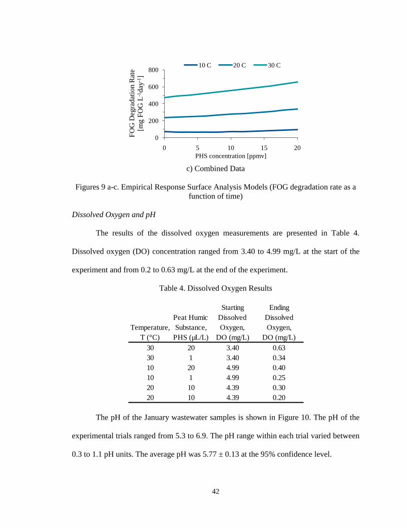
Figures 9 a-c. Empirical Response Surface Analysis Models (FOG degradation rate as a function of time)
Dissolved Oxygen and pH
The results of the dissolved oxygen measurements are presented in Table 4.
Dissolved oxygen (DO) concentration ranged from 3.40 to 4.99 mg/L at the start of the
experiment and from 0.2 to 0.63 mg/L at the end of the experiment.
Table 4. Dissolved Oxygen Results
The pH of the January wastewater samples is shown in Figure 10. The pH of the
experimental trials ranged from 5.3 to 6.9. The pH range within each trial varied between
0.3 to 1.1 pH units. The average pH was 5.77 ± 0.13 at the 95% confidence level.
0
200
400
600
800
0 5 10 15 20
FOG
Deg
rada
tion
Rat
e[m
g FO
G L
-1da
y-1]
PHS concentration [ppmv]
10 C 20 C 30 C
Starting Ending
Temperature, Peat Humic Substance,
Dissolved Oxygen,
Dissolved Oxygen,
T (°C) PHS (µL/L) DO (mg/L) DO (mg/L)30 20 3.40 0.6330 1 3.40 0.3410 20 4.99 0.4010 1 4.99 0.2520 10 4.39 0.3020 10 4.39 0.20

43
Figure 10. January Wastewater Sample Bioreactor pH (Compilation of all experiments)
Aqueous and Atmospheric Hydrogen Sulfide
The concentration of aqueous hydrogen sulfide, H2Saq, measurements ranged
from 4.6 to 12.5 mg/L. Data indicated that the fluctuations in aqueous sulfide
concentration in both control and PHS-supplemented bioreactors were statistically
identical. Figure 11 is an example of the aqueous sulfide concentration between a control
and PHS-supplemented bioreactor. For temperatures of 20-30°C, each set of side-by-side
experiments exhibited the highest H2Saq concentration at the beginning of the experiment
followed by a sharp decrease and subsequent smaller fluctuations in concentration.
4
5
6
7
8
0.0 1.0 2.0 3.0 4.0 5.0
pH
Time [days]

44
Figure 11. July Wastewater Sample H2Saq Concentration (T = 20°C, PHS = 10 ppm(v), 0 (Control))
The atmospheric hydrogen sulfide concentration measurements ranged from 2 to
60 ppm(v). Similar to the aqueous hydrogen sulfide data, the atmospheric hydrogen
sulfide concentration was highest at the beginning of the experiment and was followed by
an initial sharp decrease. Smaller fluctuations and a gradual increase in atmospheric
sulfide concentration were observed for temperatures of 20°C and 30°C. At an operating
temperature of 10°C, atmospheric sulfide was below the detection limits of the
equipment. At temperatures of 20°C and 30°C, the PHS-supplemented bioreactors
produced more atmospheric hydrogen sulfide in a range of 1.8 to 3.2 ppm(v) greater than
the control as shown in Figure 12.
0.0
2.0
4.0
6.0
8.0
10.0
12.0
0 0.5 1 1.5 2 2.5 3 3.5
H2S
aq[m
g S2-
L-1]
Time [days]
Control PHS-supplemented

45
Figure 12. July Wastewater Sample H2Satm Concentration (T = 20°C, PHS = 10 ppm(v), 0 (Control))
Cell Counts
Table 5 lists the results for the viable CFU concentration (CFU/mL) for
experiments from the July wastewater samples. The concentrations are reported for a
temperature range of 20°C to 30°C and a PHS concentration range of 0 to 20 ppm(v). The
increase in viable cell concentration in the bioreactors ranges from 12 to 102 times more
than the original starting concentration. The data indicate increasing PHS concentration
and temperature both increase the viable colony forming units in the bioreactor.
Table 5. July Wastewater Sample Microorganism Counts
0.0
2.0
4.0
6.0
8.0
0.00 0.50 1.00 1.50 2.00 2.50 3.00 3.50
H2S
atm
[ ppm
(v)]
Time [days]
Control PHS-supplemented
Detection Limits Surpassed
Temperature, PHS, start end
(°C) (µL/L) CFU mL-1 CFU mL-1 per Trial Ratio1 2.7E+04 1.6E+06 58
20 3.5E+04 3.6E+06 1020 (Control) 4.1E+04 5.3E+05 12
10 2.9E+04 1.1E+06 3720
Viable CFU Concentration, Concentration
Increase,
1.8
3.1
30

46
4.2 Grease Interceptor Material Experiment
Grease interceptor material experiments were conducted at 25°C and 5% grease in
tap water by volume.
Fog Degradation Analysis
Bioreactors were tested to ensure their equivalency by running two control
reactors side by side. The results of the equivalency test are shown in Figure 13.
Figure 13. Bioreactor Equivalency Experiment (5% (vol.) Grease, T = 25°C, PHS = 0 (Control))
The figure indicates no significant difference (95% confidence level) exists
between bioreactors. Bioreactor experiments were performed side by side with bioreactor
controls. Therefore all experimental results are reported as ratios of FOG degradation
rates affected by PHS relative to FOG degradation rates from control bioreactors. Figure
14 is an example of experimental results from a side-by-side experiment and control.
0
4000
8000
12000
16000
0.0 1.0 2.0 3.0 4.0 5.0 6.0
FOG
Con
cent
ratio
n[m
g FO
G L
-1]
Time [days]
Control Control

47
Figure 14. Grease Interceptor Experiments 9 & 10 (5% (vol.) Grease, T = 25°C, PHS = 500 ppm(v), 0(Control))
A significant difference (95% confidence level) exists in the FOG concentration
as a function of time in the control bioreactor and the PHS dosed bioreactor. Figure 14
shows an initial increase in FOG concentration which is also observed in the majority of
FOG degradation experiments. The results of the replicate experiments are presented in
Table 6. The measured ratios of FOG degradation rate varied from 0.9 to 2.2.
Table 6. Grease Interceptor FOG Degradation Results
0
4000
8000
12000
16000
0.0 1.0 2.0 3.0
FOG
Con
cent
ratio
n[m
g FO
G L
-1]
Time [days]
Control PHS
Reactor Trial,
Peat Humic Substance,
FOG Degradation Rate,
FOG Degradation Rate,
Designation PHS (µL L-1) mg FOG L-1 d-1 RatioG8 0 756G7 500 1322G9 0 2320G10 500 3471G11 0 2167G12 500 2367G13 0 1429G14 500 1303G16 0 1814G17 500 4011
2.2
1.7
1.5
1.1
0.9

48
Cell Counts
Cell count samples were acquired at the start and end of the experiments. Table 7
is a typical set of cell count data for an experiment.
Table 7. Grease Interceptor Microorganism Counts
The increase in CFU concentration ranges from 18.7 to 82.5 times more than the
original starting concentration. The data indicate the rate of cell growth in the PHS-dosed
bioreactor is approximately 4.5 times greater relative to the control.
Experiment,Colony Forming
Unit Concentration,Concentration
Increase,Reactor Sample CFU mL-1 per trial
Start 7.87E+04End 1.55E+06Start 4.25E+04End 3.55E+06
Control 18.7
PHS 82.5

49
Chapter 5: Discussion
This work is an investigation of the degradation of fats, oils and grease and
reduction of hydrogen sulfide in domestic wastewater collection systems and commercial
grease interception systems. The results are discussed here with reference to available
literature related to FOG degradation and microbial activity in wastewater.
5.1 Domestic Wastewater Study
FOG Degradation
The rate of FOG degradation was selected as a characteristic for the evaluation of
peat humic substance additive performance. Degradation, in this work, is defined as a
breakdown of molecules into smaller molecules or decomposition of a compound by
stages; exhibiting well-defined intermediate products. An increase in FOG concentration
from the initial FOG concentration as measured by the InfraCal™ infrared detector was
observed in most experiments as shown in Figure 7. The results suggest that this is a
beginning stage of FOG degradation and may be the result of both the reduction of FOG
particle size and increase in FOG bioavailability. One possible explanation for the
reduction in particle size may be the mixing intensity (applying shearing force) coupled
with the release of extracellular enzymes such as lipases or hydrolases, initially reduced
FOG particle size and increased the concentration of free lipids and fatty acids. Smaller
particles have a high surface area to volume ratio and offer a larger surface area for
bacterial colonization [27]. Smaller FOG particles are also more soluble in hexane due to
the larger surface area were found to be more easily detected by the method of
quantification used in this work. Literature also suggests that under anaerobic conditions,
it is also likely for microbial activity to produce more fermentable material than is

50
consumed [17]. This increase in concentration is also consistent with an observed lag
phase approximately 24 hours in length before a reduction in FOG concentration. This is
consistent with literature reporting a lag phase of approximately 24 hours before
significant degradation of FOG material [13]. However, some experiments exhibited no
lag phase. This might suggest that microbial flora present in the bioreactors had been
acclimatized to their environment. Microbes that have acclimatized may not exhibit
evidence of a developmental lag phase [16].
Dissolved Oxygen and pH
The dissolved oxygen concentration was initially observed to be under aerobic
conditions and proceed to or approach anaerobic conditions for bioreactor trials in which
DO was measured listed in Table 4. The high content of FOG may contribute to high
chemical and biological oxygen demand. Reported rates for oxygen uptake rates in
domestic sewage have been reported in a range from 2 to 20 mg L-1 h-1 with an average
rate of 14 L-1 h-1. For the 2 L experimental system it may be reasonable to assume that the
time taken to transition between aerobic and anaerobic microbial respiration was less than
24 hours [10]. The role of PHS in the stimulation of microorganisms may change during
the aerobic-anaerobic transition however it is reported to have positive effects in each
regime [29]. The pH was observed to range between 5.3 and 6.9 for bioreactor trials in
which pH was measured as shown in Figure 10. An average pH of 5.77 indicated the
biodegradation experiments took place in a slightly acidic environment. This pH range
suggests that the experimental medium has been subject to microbial activity, particularly
organic matter fermentation [4], [12]. In this range of pH the production and quantity of
hydrogen sulfide are near maximum [11].

51
Aqueous and Atmospheric Hydrogen Sulfide
The measured aqueous and atmospheric hydrogen sulfide concentrations were
difficult to analyze. Aqueous phase H2S concentrations were measureable, however their
degree of fluctuation as shown in Figures 11 and 12 did not allow for meaningful
interpretation. One possible explanation for the high initial H2Saq concentrations detected
in most experiments may be due to the activity of sulfate reducing bacteria during sample
storage. The subsequent sudden decrease and fluctuation of H2Saq may be caused by
equalization with H2Satm upon vigorous agitation. Sulfide concentration fuctuation may
also be caused by microbial activity involving microbial sulfate reduction and sulfide re-
oxidation cycles [19], [37].
The generation of atmospheric H2S was observed over the full range of the
experimental detection system; however, no H2Satm was detected at a temperature of
10°C. It is hypothesized that H2Saq did not evolve from the aqueous phase in detectable
quantities due to high solubility at low temperature, or increased gaseous density
prevented detectable quantities of H2Satm from entering the analysis stream. In agreement
with H2Saq measurements, a high initial concentration was detected for experimental
temperatures 20°C and 30°C followed by a sudden decrease. The initial trend in H2Satm
concentration may correspond to the initial non-equilibrium of aqueous hydrogen sulfide
and intense agitation may have facilitated degassing of the saturated aqueous medium.
Continuing after the initial concentration trend, a gradual increase in H2Satm
concentration was observed for experimental temperatures of 20°C and 30°C which is
attributed to the activity of sulfate reducing bacteria. SRB inhabit many aquatic and
terrestrial environments that transition between aerobic and anaerobic conditions [10],

52
[11]. High PHS dosed reactors produced more H2Satm than low PHS dosed reactors and
controls. Literature studies indicate humic substances are capable of both providing both
electron accepting and donating capability for organisms for highly oxidized and reduced
humic substances, respectively [37]. The capability of humic substances to bind, create
complexes with, and increase the organic partitioning coefficient is also well-documented
[30]. It is hypothesized that due to the possible high chemical oxygen demand exerted on
the medium, the addition of PHS provided a degree of stimulation by three mechanisms.
Initially, PHS functioned as an electron acceptor, replacing sulfate as a terminal electron
acceptor for microbial respiration. In the second mechanism, PHS increased the solubility
of sulfur-containing organic compounds, and created PHS-sulfur organic compound
complexes. Once reduced, PHS functioned as a thermodynamically favorable electron
donor, increasing the short term availability of an easily fermentable sulfur-containing
substrate.
Cell Counts
Colony-forming microorganism concentration measurements were performed for
the July wastewater sample for organisms limited to aerobic conditions capable of
growing on a nutrient-rich media. It was observed that the rate of cell growth increased as
a function of PHS concentration and temperature. These results shown in Table 5 were
expected and consistent with available literature.
Experimental Design Analysis
The experimental design analysis of FOG degradation rate as a function of PHS
and temperature found that both factors significantly impacted the degradation rate in
wastewater samples. Temperature and PHS were both expected to contribute to FOG

53
degradation. As shown in Table 2, the highest observed rates of FOG degradation for
each wastewater sample occurred at high temperature and high doses of PHS. Therefore,
it is inferred that the optimal conditions for FOG degradation were outside of the
parameter ranges tested. The highest FOG degradation rate,
721 mg FOG L-1 day-1 or 0.03 g FOG L-1 h-1, compares well with the pilot and industrial
scale study of Grulois et al. (1993). For semi-continuous processes treating grease
residue, a special consortium of biomass was found to degrade lipids between 0.03 and
0.04 g FOG L-1 h-1 in a mesophilic temperature range of 25 to 30°C [38]. A first order
kinetic model was applied to calculate the apparent degradation rate constant, k, as a
measure of the rate of biochemical degradation [39]. The k values ranged from 0.02 day-1
at a temperature of 10°C to 0.25 day-1 at 30°C. These values are close to the accepted
typical values for municipal wastewater (0.17 day-1) and petroleum oils (0.11 day-1) [40].
Wastewater samples collected during January were found to have lower FOG degradation
rates compared to wastewater samples collected during July for the same experimental
conditions. These results indicate that the samples may have contained different
microbial communities. For wastewater samples collected in January, it was additionally
found that the interaction of temperature and PHS concentration is significant for FOG
degradation. This would suggest the increased microbial activity associated with high
temperatures caused a larger response toward PHS as a degradation stimulant. It has been
observed in both wastewater samples that the temperature is a more significant parameter
in enhancing biological FOG degradation. Warmer temperatures allow for the increased
microbial activity due to increased solubility and subsequent bioavailability of FOG and
also reduction in the amount of energy required for microorganism activity [41]. For
54
wastewater samples collected in July, it was additionally observed that the second order
effect of temperature significantly impacted FOG degradation. One possible explanation
for this is that the microbial community contained in the July wastewater sample was
more sensitive to temperature changes in the range tested. Microbial communities will
perform optimally in environments similar to those in which they have been acclimatized
[12]. Tolerance for temperature shock and performance of biodegradation after
adjustment varies among mixed microbial communities [18]. Empirical models were
created for predicting FOG degradation rates in wastewater as a function of temperature
and PHS concentration for application to field trials. The models suggest that PHS has a
greater effect on microbial activity in the January wastewater sample and also has a
greater effect at high temperature. This may also be explained by the interaction between
temperature and PHS on biodegradation.
5.2 Grease Interceptor Material Experiment
FOG Degradation
Bioreactors were tested to ensure their equivalency by running control (no PHS)
experiments. No significant difference between FOG degradation in the bioreactors exists
at the 95% confidence level. For most FOG degradation experiments the trends observed
for FOG concentration as a function of time included a characteristic initial increase in
concentration followed by a period of decreasing concentration as shown in Figure 14.
The mechanism as described for FOG degradation in wastewater experiments previously
discussed is likely to also apply to these experiments. FOG degradation rates for PHS-
dosed reactors ranged from 0.9 to 2.2 times greater than control reactors. The average
apparent degradation rate constant was found to be 0.24 ± 0.10 day-1 at the 95%

55
confidence interval which is between rate constants reported for municipal wastewater
(0.17) and edible oils (0.35) [40]. The large differences observed between comparisons of
FOG degradation rates are suggested to be a function of differences in sample preparation
and storage. Different storage periods and numbers of warming cycles are hypothesized
to have changed the properties of the microbial consortium and FOG substrate present in
each sample [9], [41].
Cell Counts
The results of the grease material study cell counts listed in Table 7 have
indicated that PHS may stimulate the rate of cellular growth on grease material substrate
by up to a factor of 4 to 5, relative to a control. Large variations were observed between
trials; most are considered to be a function of sample preparation.
5.3 Experimental Limitations
Extensive care was taken in preparation of the collected data yet high variability
was observed in some measurements. This is suggested to be due to the limitations of the
experimental system and procedures. It is important to note that this work did not include
chemical analysis and characterization of the FOG samples or peat humic substance.
Thus, the changes in chemical composition of the FOG material is not known, nor the
concentration of PHS during experimentation. Preliminary analyses have identified the
mixed microbial cultures acquired from wet well and grease interceptor grab samples as
another source of performance variability. The peat humic substance product
was also found to contain an average microorganism concentration in a range of
1.85 x 10⁴ CFU mL-1. Given that wastewater experiments used PHS in a range of
2 to 40 μL, it is unlikely that any colony forming units could compete with established

56
microorganisms. Grease interceptor material experiments used a PHS dosage of 1 mL
which may have contributed to the FOG degradation performance.

57
Chapter 6: Conclusions & Recommendations
The effects of peat humic substance on the rate of FOG degradation in wastewater
and grease interceptor materials were studied. The effects of PHS on wastewater pH,
dissolved oxygen and hydrogen sulfide concentrations were also investigated in a well-
mixed, controlled, batch laboratory bioreactor. Samples used for all experimentation were
provided by JSH International including peat humic substance (PHS), grease interceptor
and domestic wastewater materials.
For experiments using domestic wastewater, an experimental design was used to
investigate the effects of PHS concentration and temperature on FOG degradation. It was
found that the FOG degradation rate increased as a function of temperature and PHS
concentration and ranged from 10% to 110% relative to control experiments. The data
suggest that FOG degradation in these systems proceeds by a two-part biological
mechanism involving increasing FOG bioavailability and FOG consumption. The
mechanism suggests activity of microorganisms breaks down large FOG molecules and
particles initially which is consistent with an observed increase in FOG concentration.
This is followed by consumption of smaller FOG molecules and subsequent decrease in
FOG concentration. In the experiments using grease interceptor material, the results again
supported this two-part mechanism. For grease interceptor material experiments at
constant temperature, peat humic substance enhanced FOG degradation rates by up to
120% relative to control experiments. The addition of PHS also increased the growth rate
of microorganisms during both wastewater and grease interceptor experiments by up to a
factor of 3 and 4, respectively. Peat humic substance was observed to have no effect on
the concentration of aqueous hydrogen sulfide, however, increases in hydrogen sulfide
58
concentration were observed in correspondence with high PHS dosing. Thus, it appears
that the PHS products enhance microbial metabolic activity, leading to enhanced FOG
degradation rates and H2Satm generation.
The results of this work have led to several recommendations for further research.
Larger scale experimentation, particularly in commercial grease interception systems and
domestic wastewater collection systems is needed before peat humic substance additives
can be optimally applied in industrial applications. It is recommended that a similar
scaled-up study be performed with several method revisions in order to more confidently
quantify and describe the effects of peat humic substances in wastewater systems. Futher
experiments to verify hypotheses concerning biological degradation of FOG may include
add-back studies in which non-sterile and sterile experiments are compared side-by-side.
Other recommendations include the use of a standardized and robust microbial culture,
use of real-time investigation of microbial activity based on gene and protein expression,
use of well-defined aqueous media, improvement of water-quality parameter
measurement and improvement of characterization and quantification techniques for both
FOG and PHS.

59
References
[1] G. Tchobanoglous, F. L. Burton, and H. D. Stensel, Wastewater Engineering: Treatment and Reuse. New York, NY: McGraw-Hill, 2003.
[2] W. Miller and R. M. Miller, Environmental Hazards - Liquid Wastes: A Bibliography. Monticello, IL: Vance Bibliographies, 1985.
[3] H. K. Shon et al., "Degradation of Fat, Oil, and grease (FOGs) by Lipase-producing Bacterium Pseudomonas sp. Strain D2D3," Journal of Microbiology and Biotechnology, vol. 12, pp. 583-591, 2002.
[4] J. J. Ducoste, K. M. Keener, J. W. Groninger, and L. M. Holt, "Assessment of Grease Interceptor Performance," Water Environment Research Foundation, Alexandria, VA, Technical Report 2008.
[5] O. Da-Silva and E. Alpay, "Removal of Organic Pollutants from Wastewater Using Humic Substances," Water Resources Management II, vol. 8, pp. 125-134, 2003.
[6] W. H. Hager, "Wastewater Hydraulics: Theory and Practice," Berlin, 1999.
[7] R. Southerland, "Sewer Fitness: Cutting the Fat," American City and Country, vol. 117, no. 15, pp. 27-31, 2002.
[8] S. Okabe, T. Ito, H. Satoh, and Y. Watanabe, "Effect of Nitrite and Nitrate on Biogenic sulfide Production in Sewer Biofilms Determined by the Use of Microelectrodes," Water Science and Technology, vol. 47, no. 11, pp. 281-288, 2003.
[9] M. Cammarota and D. Freire, "A Review on Hydrolytic Enzymes in the Treatment of Wastewater with High Oil and Grease Content," Bioresource Technology, vol. 97, pp. 2195-2210, 2006.
[10] A. G. Boon, "Septicity in Sewers: Causes, Consequences and Containment," Water Science and Technology, vol. 31, no. 7, pp. 237-253, 1995.
[11] S. Delgado, M. Alvarez, L. E. Rodriguez-Gomez, and E. Aguiar, "H2S Generation in a Reclaimed Urban Wastewater Pipe. Case Study: Tenerife (Spain)," Water Research, vol. 69, pp. 539-547, 1999.

60
[12] G. Vidal, A. Carvalho, R. Mendez, and J. A. Lema, "Influence of the Content in Fats and Proteins on the Anaerobic Biodegradability of Dairy Wastewaters," Bioresource Technology, vol. 74, pp. 231-239, 2000.
[13] N. Wakelin and C. Forster, "An Investigation into Microbial Removal of Fats, Oils and Greases," Bioresource Technology, vol. 59, pp. 37-43, 1997.
[14] L. Maya-Altamira, A. Baun, I. Angelidaki, and J. E. Schmidt, "Influence of Wastewater Characteristics on Methane Potential in Food-processing Industry Wastewaters," Water Research, vol. 42, pp. 2195-2203, 2008.
[15] N. A. Campbell and J. B. Reece, Biology 7th ed. San Francisco, California, United States of America: Benjamin Cummings, 2005, ch. 1, pp. 75-76.
[16] T. Shigematsu et al., "Microbial Diversity of Mesophilic Methanogenic Consortium that can Degrade Long-chain Fatty Acids in Chemostat Cultivation," Journal of Bioscience, vol. 102, no. 11, pp. 535-544, 2006.
[17] T. Hvitved-Jacobsen, J. Vollertsen, and J. S. Matos, "The Sewer as a Bioreactor - A Dry Weather Approach," Water Science and Technology, vol. 45, no. 3, pp. 11-24, 2002.
[18] M. T. Madigan and J. M. Martinko, Brock Biology of Microorganisms 11th ed. Upper Saddle River, United States of America: Pearson Prentice Hall, 2006.
[19] J. K. Keller, P. B. Weisenhorn, and J. P. Megonigal, "Humic Acids as Electron Acceptors in Wetland Decomposition," Soil Biology and Biotechnology, vol. 41, pp. 1518-1522, 2009.
[20] M. Perle, K. Shlomo, and G. Shelef, "Some Biochemical Aspects of the Anaerobic Degradation of Dairy Wastewater," Water Research, vol. 29, no. 6, pp. 1549-1554, 1995.
[21] K. H. Tan and C. O. Gill, "Effect of Culture Conditions on Batch Growth of Saccharomycopsis Lipolytica on Olive Oil," Applied Microbiology, vol. 20, pp. 201-206, 1984.
[22] K. H. Tan and C. O. Gill, "Batch Growth of Saccharomycopsis Lipolytica on Animal Fats," Applied Microbiology, vol. 21, pp. 292-298, 1985.

61
[23] D. Vieira, E. Servulo, and M. Cammarota, "Degradation Potential and Growth of Anaerobic Bacteria in Produce Water," Environmental Technology, vol. 26, pp. 915-922, 2005.
[24] J. H. van der Graaf, J. M. de Koning, A. Ravazzini, and V. Miska, "Treatment Matrix for Reuse of Upgraded Wastewater," Water Science and Technology, vol. 5, no. 1, pp. 87-94, 2005.
[25] R. M. Ashley, T. Hvitvd-Jacobsen, and J. L. Bertrand-Krajewski, "Quo Vadis Sewer Process Modelling," Water Science and Technology, vol. 39, no. 9, pp. 9-22, 1999.
[26] B. K. Reese, M. A. Anderson, and C. Amrhein, "Hydrogen Sulfide Production and Volatization in a Polymictic Eutrophic Saline Lake, Salton Sea, California," The Science of the Total Environment, vol. 046, pp. 205-218, 2008.
[27] L. Masse, K. J. Kennedy, and S. Chou, "Testing of Alkaline and Enzymatic Hydrolysis Pretreatments for Fat Particles in Slaughterhouse Wastewater," Bioresouce Technology, vol. 77, pp. 145-155, 2001.
[28] Y. Laor and M. Rebhun, "Evidence for Non-linear Binding of PAHs to Dissolved Humic Acids," Environmental Science and Technology, vol. 36, no. 5, pp. 955-961, 2002.
[29] H. A. Hartung, "Stimulation of Anaerobic Digestion with Peat Humic Substance," The Science of the Total Environment, vol. 113, pp. 17-33, 1992.
[30] S. Matsui, H. Yamamoto, Y. Shimizu, J. Harada, and D. Einaga, "Humic Substances Affecting the Limitation of the Activated Sludge Process for Removal of Micropollutants," Water Science and Technology, vol. 38, no. 7, pp. 217-225, 1998.
[31] D. R. Lovley, J. D. Coates, E. L. Blunt-Harris, E. J. P. Phillips, and J. C. Woodward, "Humic Substances as Electron Acceptors for Microbial Respiration," Letters to Nature, vol. 382, pp. 445-448, 1996.
[32] Wilks Enterprise Inc. (2009, April) Wilks Enterprise Inc. Web site. [Online]. http://www.wilksir.com
[33] Wilks Enterprise Inc. (2009, April) Wilks Enterprise Inc. Web site. [Online]. http://www.wilksir.com/oilgrease-analyzers
[34] W. A. Telliard, Method 1664, Revision A. Washington, DC, Maryland, United States of America: United States Environmental Protection Agency, 2010.

62
[35] D. C. Montgomery, G. C. Runger, and N. F. Hubele, "Design of Engineering Experiments," in Engineering Statistics 3rd ed. Hoboken, New Jersey, United States of America: John Wiley & Sons, 2006.
[36] J. D. Cline, "Spectrophotometric Determination of Hydrogen Sulfide in Natural Waters," Limnology and Oceanography, vol. 14, no. 3, pp. 454-458, 1969.
[37] S. Minderlein and C. Blodau, "Humic-rich Peat Extracts Inhibit Sulfate Reduction, Methanogenesis and Anaerobic Respiration but not Acetogenesis in Peat Soils of a Temperate Bog," Soil Biology and Biochemistry, vol. 42, pp. 2078-2086, 2010.
[38] P. Becker et al., "The Biodegradation of Olive Oil and the Treatment of Lipid-rich Wool Scouring Wastewater Under Aerobic Thermophilic Conditions," Water Research, vol. 33, no. 3, pp. 653-660, 1999.
[39] J. Kudo, K. Kobayashi, K. Marumo, and T. Yoshinori, "Fluctuation in Proteinaceous Labile Organic Matter Verified with Degradation Rate Constants of Terrestrial Biochemical Indicators," Organic Geochemistry, vol. 37, pp. 1655-1663, 2006.
[40] J. C. Groenwold, R. F. Pico, and K. S. Watson, "Comparison of BOD Relationships for Typical Edible and Petroleum Oils," Water Pollution Control Federation, vol. 54, no. 4, pp. 398-405, 1982.
[41] G. Nakhla, M. Al-Sabawi, A. Bassi, and V. Liu, "Anaerobic Treatability of High Oil and Grease Rendering Wastewater," Journal of Hazardous Materials: B, vol. 102, pp. 243-255, 2003.

63
Appendices
64
Appendix A: Experimental Data
Table 8. January Sample Wastewater FOG Data
Run
#
Sam
ple
Time Days a1 a2 a3 d1 d2 T n1 n2 n3 tav stdev t stat A IR_Av F conav Sdev %SD % Dec. Dif.Slope
[ppm/D]Cycle
Regrssn.Design Code 1,1 1 1/6/10 1:05 PM 0.00 141 134 207 66 7 207 141 134 FALSE 137.5 4.9 19.86 137.5 1301 381 29.3% 0%Vessel T [C] 30 2 1/7/10 10:35 AM 0.90 222 159 134 63 25 222 FALSE 159 134 146.5 17.7 6.04 171.7 1624 429 26.4% -25% -25% 360.8 -590
Agitation [rpm] 1100 3 1/8/10 10:35 AM 1.90 72 77 98 21 5 98 72 77 FALSE 74.5 3.5 9.40 82.3 779 131 16.8% 40% 65% -845.2PHS [ppmv] 20 4 1/9/10 8:30 PM 3.31 19 19 17 0 2 17 19 19 FALSE 19 0.0 #DIV/0! 18.3 173 11 6.3% 87% 47% -428.5
5 1/10/10 10:15 PM 4.38 16 12 12 4 0 16 FALSE 12 12 12 0.0 #DIV/0! 13.3 126 22 17.3% 90% 4% -44.16 1/11/10 11:20 AM 4.93 19 16 12 3 4 12 19 16 FALSE 17.5 2.1 3.67 15.7 148 33 22.4% 89% -2% 40.5
Design Code 1,-1 1 1/6/10 1:05 PM 0.00 100 109 124 15 9 124 100 109 FALSE 104.5 6.4 4.33 111.0 1050 115 10.9% 0%Vessel T [C] 30 2 1/7/10 10:35 AM 0.90 93 114 48 21 45 48 93 114 FALSE 103.5 14.8 5.29 85.0 804 319 39.7% 23% 23% -274.6 -327
Agitation [rpm] 1100 3 1/8/10 10:35 AM 1.90 88 99 87 11 1 99 88 FALSE 87 87.5 0.7 23.00 87.5 828 63 7.6% 21% -2% 23.7PHS [ppmv] 1 4 1/9/10 8:30 PM 3.31 42 37 37 5 0 42 FALSE 37 37 37 0.0 #DIV/0! 38.7 366 27 7.5% 65% 44% -326.9
5 1/10/10 10:15 PM 4.38 13 19 15 4 2 19 13 FALSE 15 14 1.4 5.00 15.7 148 29 19.5% 86% 21% -202.86 1/11/10 11:20 AM 4.93 9 12 9 3 0 12 9 FALSE 9 9 0.0 #DIV/0! 10.0 95 16 17.3% 91% 5% -98.3
Design Code -1,-1 1 1/11/10 5:45 PM 0.00 57 98 118 20 41 57 FALSE 98 118 108 14.1 5.10 91.0 861 294 34.2% 0%Vessel T [C] 10 2 1/12/10 1:45 PM 0.83 106 84 105 1 21 84 106 FALSE 105 105.5 0.7 43.00 105.5 998 118 11.8% -16% -16% 164.6 -42
Agitation [rpm] 1100 3 1/13/10 3:20 PM 1.90 109 20 76 33 56 20 109 FALSE 76 92.5 23.3 4.39 68.3 646 426 65.8% 25% 41% -329.9PHS [ppmv] 1 4 1/14/10 3:20 PM 2.90 112 92 85 20 7 112 FALSE 92 85 88.5 4.9 6.71 96.3 911 133 14.5% -6% -31% 264.9
5 1/15/10 12:05 PM 3.76 117 99 76 18 23 76 117 99 FALSE 108 12.7 3.56 97.3 921 194 21.1% -7% -1% 10.96 1/16/10 8:40 PM 5.12 84 88 59 4 25 59 84 88 FALSE 86 2.8 13.50 86.0 814 149 18.3% 5% 12% -79.07 1/17/10 9:05 AM 5.64 50 53 50 3 0 53 50 FALSE 50 50 0.0 #DIV/0! 51.0 482 16 3.4% 44% 38% -640.0
Design Code -1,1 1 1/11/10 5:45 PM 0.00 54 19 76 22 35 19 54 FALSE 76 65 15.6 4.18 49.7 470 272 57.9% 0%Vessel T [C] 10 2 1/12/10 1:45 PM 0.83 85 53 61 24 8 85 FALSE 53 61 57 5.7 7.00 66.3 628 158 25.1% -34% -34% 189.2 -25
Agitation [rpm] 1100 3 1/13/10 3:20 PM 1.90 68 64 56 4 8 56 68 64 FALSE 66 2.8 5.00 62.7 593 58 9.8% -26% 7% -32.5PHS [ppmv] 20 4 1/14/10 3:20 PM 2.90 56 66 61 5 5 FALSE 56 66 61 61 5.0 #VALUE! 61.0 577 47 8.2% -23% 3% -15.8
5 1/15/10 12:05 PM 3.76 79 65 58 14 7 79 FALSE 65 58 61.5 4.9 5.00 67.3 637 101 15.9% -36% -13% 69.36 1/16/10 8:40 PM 5.12 51 56 41 5 10 41 51 56 FALSE 53.5 3.5 5.00 49.3 467 72 15.5% 1% 36% -125.47 1/17/10 9:05 AM 5.64 39 33 36 3 3 FALSE 39 33 36 36 3.0 #VALUE! 36.0 341 28 8.3% 28% 27% -243.8
Design Code 0,0 1 1/19/10 7:15 PM 0.00 423 433 479 46 10 479 423 433 FALSE 428 7.1 10.20 445.0 4210 283 6.7% 0%Vessel T [C] 20 2 1/20/10 10:20 AM 0.63 507 495 640 133 12 640 507 495 FALSE 501 8.5 23.17 501.0 4740 761 16.1% -13% -13% 843.0
Agitation [rpm] 1150 3 1/21/10 10:55 AM 1.65 636 580 572 56 8 636 FALSE 580 572 576 5.7 15.00 576.0 5449 330 6.1% -29% -17% 692.7PHS [ppmv] 10 4 1/22/10 9:30 AM 2.59 578 464 700 122 114 700 578 464 FALSE 521 80.6 3.14 580.7 5494 1117 20.3% -30% -1% 46.9
5 1/23/10 5:30 PM 3.93 715 666 770 55 49 770 715 666 FALSE 690.5 34.6 3.24 717.0 6783 492 7.3% -61% -31% 967.46 1/24/10 11:40 AM 4.68 756 652 732 24 80 652 756 FALSE 732 744 17.0 7.67 713.3 6749 515 7.6% -60% 1% -45.8
Design Code 0,0 1 1/19/10 7:15 PM 0.00 414 385 382 29 3 414 FALSE 385 382 383.5 2.1 20.33 383.5 3628 167 4.6% 0%Vessel T [C] 20 2 1/20/10 10:20 AM 0.63 700 500 508 192 8 700 FALSE 500 508 504 5.7 49.00 504.0 4768 1071 22.5% -31% -31% 1814.0
Agitation [rpm] 1150 3 1/21/10 10:55 AM 1.65 650 708 640 58 10 708 650 FALSE 640 645 7.1 12.60 666.0 6301 347 5.5% -74% -42% 1496.3 -294PHS [ppmv] 10 4 1/22/10 9:30 AM 2.59 614 588 636 22 26 588 614 FALSE 636 625 15.6 3.36 612.7 5796 227 3.9% -60% 14% -536.2
5 1/23/10 5:30 PM 3.93 600 566 612 12 34 566 600 FALSE 612 606 8.5 6.67 592.7 5607 226 4.0% -55% 5% -141.96 1/24/10 11:40 AM 4.68 540 532 570 30 8 570 540 532 FALSE 536 5.7 8.50 547.3 5178 190 3.7% -43% 12% -566.6
E6
E4
E3
E1
E2
E5

65
Table 9. July Sample Wastewater FOG Data
Run
#
Sam
ple
Time Days a1 a2 a3 d1 d2 T n1 n2 n3 tav stdev t stat A IR_Av F conav Sdev %SD % Dec. Dif.Slopes
[ppm/D]Cycle
Regrssn.1 7/15/10 9:45 PM 0.56 337 320 368 31 17 368 337 320 FALSE 328.5 12.0 4.65 341.7 3232 230 7% 0%
Vessel T [C] 30 2 7/16/10 11:15 AM 0.00 319 305 384 65 14 384 319 305 FALSE 312 9.9 10.29 336.0 3179 399 13% 2% 2% 95.3Agitation [rpm] 1000 3 7/16/10 10:20 PM 0.46 345 364 332 19 13 364 345 FALSE 332 338.5 9.2 3.92 347.0 3283 152 5% -2% -3% 225.4
PHS [ppmv] 20 4 7/17/10 10:30 AM 0.97 546 414 354 132 60 546 FALSE 414 354 384 42.4 5.40 438.0 4144 929 22% -28% -27% 1698.3 -7215 7/17/10 10:30 PM 1.47 353 372 424 52 19 424 353 372 FALSE 362.5 13.4 6.47 383.0 3623 348 10% -12% 16% -1040.76 7/18/10 10:30 AM 1.97 434 359 350 75 9 434 FALSE 359 350 354.5 6.4 17.67 354.5 3354 436 13% -4% 8% -539.37 7/18/10 10:00 PM 2.45 398 336 350 48 14 398 FALSE 336 350 343 9.9 7.86 361.3 3418 308 9% -6% -2% 134.98 7/19/10 10:00 AM 2.95 283 240 248 35 8 283 FALSE 240 248 244 5.7 9.75 257.0 2431 216 9% 25% 31% -1974.19 7/19/10 10:45 PM 3.48 261 222 39 39 FALSE 261 222 241.5 27.6 #VALUE! 241.5 2285 261 11% 29% 5% -276.01 7/15/10 9:45 PM 0.56 362 328 286 34 42 286 362 328 FALSE 345 24.0 3.47 325.3 3078 360 12% 0%
Vessel T [C] 30 2 7/16/10 11:15 AM 0.00 419 274 320 99 46 419 FALSE 274 320 297 32.5 5.30 337.7 3195 701 22% -4% -4% -207.4Agitation [rpm] 1050 3 7/16/10 10:20 PM 0.46 279 310 283 27 4 310 279 FALSE 283 281 2.8 14.50 281.0 2658 160 6% 14% 17% -1160.9
PHS [ppmv] 1 4 7/17/10 10:30 AM 0.97 431 344 326 87 18 431 FALSE 344 326 335 12.7 10.67 367.0 3472 531 15% -13% -26% 1605.0 -6365 7/17/10 10:30 PM 1.47 486 360 324 126 36 486 FALSE 360 324 342 25.5 8.00 390.0 3690 805 22% -20% -7% 435.26 7/18/10 10:30 AM 1.97 342 367 346 21 4 367 342 FALSE 346 344 2.8 11.50 351.7 3327 127 4% -8% 12% -725.37 7/18/10 10:00 PM 2.45 516 304 255 212 49 516 FALSE 304 255 279.5 34.6 9.65 358.3 3390 1312 39% -10% -2% 131.68 7/19/10 10:00 AM 2.95 215 210 213 2 3 210 215 FALSE 213 214 1.4 4.00 212.7 2012 24 1% 35% 45% -2756.29 7/19/10 10:45 PM 3.48 235 259 253 6 18 235 FALSE 259 253 256 4.2 7.00 249.0 2356 118 5% 23% -11% 647.01 7/9/10 12:30 PM 0.00 551 572 559 13 8 572 551 FALSE 559 555 5.7 4.25 560.7 5304 100 2% 0% -148
Vessel T [C] 10 2 7/9/10 11:00 PM 0.44 560 553 541 7 12 541 560 553 FALSE 556.5 4.9 4.43 551.3 5216 91 2% 2% 2% -201.8Agitation [rpm] 1050 3 7/10/10 1:55 PM 1.06 573 544 511 29 33 511 573 544 FALSE 558.5 20.5 3.28 542.7 5134 293 6% 3% 2% -131.9
PHS [ppmv] 20 4 7/10/10 11:45 PM 1.47 538 536 612 74 2 612 538 536 FALSE 537 1.4 75.00 537.0 5080 410 8% 4% 1% -130.85 7/11/10 1:00 PM 2.02 546 532 506 14 26 506 546 532 FALSE 539 9.9 4.71 528.0 4995 192 4% 6% 2% -154.26 7/11/10 11:55 PM 2.48 605 549 538 56 11 605 FALSE 549 538 543.5 7.8 11.18 564.0 5336 340 6% -1% -6% 748.87 7/12/10 11:00 AM 2.94 638 530 514 108 16 638 FALSE 530 514 522 11.3 14.50 522.0 4939 638 13% 7% 7% -860.48 7/12/10 11:30 PM 3.46 536 543 493 7 43 493 536 543 FALSE 539.5 4.9 13.29 539.5 5104 256 5% 4% -3% 317.91 7/9/10 12:30 PM 0.00 536 546 580 34 10 580 536 546 FALSE 541 7.1 7.80 554.0 5241 218 4% 0% -113
Vessel T [C] 10 2 7/9/10 11:00 PM 0.44 612 567 531 45 36 612 FALSE 567 531 549 25.5 3.50 570.0 5393 384 7% -3% -3% 346.0Agitation [rpm] 1050 3 7/10/10 1:55 PM 1.06 570 520 523 47 3 570 FALSE 520 523 521.5 2.1 32.33 521.5 4934 265 5% 6% 9% -738.3
PHS [ppmv] 1 4 7/10/10 11:45 PM 1.47 566 506 535 31 29 566 FALSE 506 535 520.5 20.5 3.14 535.7 5068 284 6% 3% -3% 327.15 7/11/10 1:00 PM 2.02 542 489 544 2 53 489 542 FALSE 544 543 1.4 54.00 543.0 5137 295 6% 2% -1% 125.76 7/11/10 11:55 PM 2.48 594 532 555 39 23 594 FALSE 532 555 543.5 16.3 4.39 560.3 5301 297 6% -1% -3% 360.57 7/12/10 11:00 AM 2.94 595 535 490 60 45 595 FALSE 535 490 512.5 31.8 3.67 540.0 5109 498 10% 3% 4% -416.68 7/12/10 11:30 PM 3.46 549 532 539 10 7 549 FALSE 532 539 535.5 4.9 3.86 540.0 5109 81 2% 3% 0% 0.01 7/1/10 12:00 PM 0.00 453 456 400 3 53 400 453 456 FALSE 454.5 2.1 36.33 454.5 4300 298 7% 0% -311
Vessel T [C] 20 2 7/1/10 9:45 PM 0.41 413 394 440 27 19 440 413 394 FALSE 403.5 13.4 3.84 415.7 3933 219 6% 9% 9% -904.3Agitation [rpm] 1000 3 7/2/10 12:00 PM 1.00 524 407 367 117 40 524 FALSE 407 367 387 28.3 6.85 432.7 4093 772 19% 5% -4% 270.9
PHS [ppmv] 10 4 7/2/10 10:25 PM 1.43 486 373 384 102 11 486 FALSE 373 384 378.5 7.8 19.55 378.5 3581 589 16% 17% 12% -1180.75 7/3/10 12:00 PM 2.00 375 398 399 1 23 375 FALSE 398 399 398.5 0.7 47.00 398.5 3770 128 3% 12% -4% 334.36 7/3/10 10:30 PM 2.44 378 394 516 122 16 516 378 394 FALSE 386 11.3 16.25 386.0 3652 714 20% 15% 3% -270.37 7/4/10 10:50 AM 2.95 546 432 414 114 18 546 FALSE 432 414 423 12.7 13.67 423.0 4002 677 17% 7% -8% 681.28 7/4/10 10:40 PM 3.44 520 439 403 81 36 520 FALSE 439 403 421 25.5 5.50 454.0 4295 567 13% 0% -7% 594.81 7/21/10 10:45 AM 0.00 374 396 437 41 22 437 374 396 FALSE 385 15.6 4.73 402.3 3806 302 8% 0% -257
Vessel T [C] 20 2 7/21/10 10:25 PM 0.49 347 349 348 1 1 FALSE 347 349 348 348 1.0 #VALUE! 348.0 3292 9 0% 14% 14% -1057.4Agitation [rpm] 1050 3 7/22/10 10:00 AM 0.97 366 352 341 14 11 366 FALSE 352 341 346.5 7.8 3.55 353.0 3340 119 4% 12% -1% 98.0
PHS [ppmv] 10 4 7/22/10 9:15 PM 1.44 529 419 393 110 26 529 FALSE 419 393 406 18.4 9.46 447.0 4229 683 16% -11% -23% 1897.25 7/23/10 10:40 AM 2.00 503 389 411 92 22 503 FALSE 389 411 400 15.6 9.36 434.3 4109 572 14% -8% 3% -214.46 7/23/10 10:15 PM 2.48 338 322 303 16 19 303 338 322 FALSE 330 11.3 3.38 321.0 3037 166 5% 20% 28% -2221.67 7/24/10 11:00 AM 3.01 329 310 331 2 19 310 329 FALSE 331 330 1.4 20.00 330.0 3122 110 4% 18% -2% 160.38 7/24/10 9:55 PM 3.47 269 307 310 3 38 269 FALSE 307 310 308.5 2.1 26.33 308.5 2919 216 7% 23% 5% -447.21 7/1/10 12:00 PM 0.00 386 342 326 44 16 386 FALSE 342 326 334 11.3 6.50 351.3 3324 294 9% 0% -278
Vessel T [C] 20 2 7/1/10 9:45 PM 0.41 383 363 308 20 55 308 383 363 FALSE 373 14.1 6.50 351.3 3324 367 11% 0% 0% 0.0Agitation [rpm] 1000 3 7/2/10 12:00 PM 1.00 457 307 314 143 7 457 FALSE 307 314 310.5 4.9 41.86 310.5 2938 801 27% 12% 12% -650.6
PHS [ppmv] 0 4 7/2/10 10:25 PM 1.43 327 297 298 29 1 327 FALSE 297 298 297.5 0.7 59.00 297.5 2815 161 6% 15% 4% -283.45 7/3/10 12:00 PM 2.00 326 263 267 59 4 326 FALSE 263 267 265 2.8 30.50 265.0 2507 334 13% 25% 9% -543.36 7/3/10 10:30 PM 2.44 268 315 300 15 32 268 FALSE 315 300 307.5 10.6 5.27 294.3 2785 227 8% 16% -8% 634.37 7/4/10 10:50 AM 2.95 341 262 304 37 42 262 341 FALSE 304 322.5 26.2 3.27 302.3 2860 374 13% 14% -2% 147.38 7/4/10 10:40 PM 3.44 307 311 320 9 4 320 307 311 FALSE 309 2.8 5.50 312.7 2958 63 2% 11% -3% 198.31 7/21/10 10:45 AM 0.00 378 409 385 24 7 409 378 FALSE 385 381.5 4.9 7.86 390.7 3696 154 4% 0% -207
Vessel T [C] 20 2 7/21/10 10:25 PM 0.49 367 349 358 9 9 FALSE 367 349 358 358 9.0 #VALUE! 358.0 3387 85 3% 8% 8% -635.8Agitation [rpm] 1050 3 7/22/10 10:00 AM 0.97 364 346 332 18 14 364 FALSE 346 332 339 9.9 3.57 347.3 3286 152 5% 11% 3% -209.1
PHS [ppmv] 0 4 7/22/10 9:15 PM 1.44 430 379 376 51 3 430 FALSE 379 376 377.5 2.1 35.00 377.5 3571 287 8% 3% -8% 608.95 7/23/10 10:40 AM 2.00 367 381 352 14 15 352 367 381 FALSE 374 9.9 3.14 366.7 3469 137 4% 6% 3% -183.36 7/23/10 10:15 PM 2.48 334 282 295 39 13 334 FALSE 282 295 288.5 9.2 7.00 303.7 2873 256 9% 22% 16% -1234.97 7/24/10 11:00 AM 3.01 314 319 351 32 5 351 314 319 FALSE 316.5 3.5 13.80 316.5 2994 190 6% 19% -3% 228.58 7/24/10 9:55 PM 3.47 294 334 349 15 40 294 FALSE 334 349 341.5 10.6 6.33 325.7 3081 269 9% 17% -2% 190.7
WW
1W
W7
WW
6W
W5
WW
4W
W3
WW
2W
W8

66
Table 10. July Sample Wastewater H2Saq and H2Satm Data
0 10 1 20 1 20 0 101 11.1 9.8 4.9 5.4 12.0 11.1 12.2 12.52 6.4 5.3 5.3 5.2 8.2 8.7 4.9 5.03 4.6 4.9 7.4 7.6 7.4 6.8 7.7 7.34 7.1 7.2 8.0 8.3 7.3 7.5 5.2 5.65 8.7 8.1 8.6 8.0 6.4 6.8 7.1 7.26 9.3 9.0 7.4 7.8 9.6 9.6 9.6 9.77 7.5 6.8 5.8 6.4 10.3 9.7 6.6 7.08 7.3 7.5 5.8 6.1 9.0 9.2 8.2 7.81 21.0 15.8 0.0 0.0 19.4 29.4 20.6 20.62 19.4 - 0.0 0.0 28.4 p/d 0.0 0.03 1.8 0.0 0.0 0.0 21.8 p/d 0.0 0.04 6.4 2.0 0.0 0.0 3.4 3.4 0.0 0.05 23.2 4.0 0.0 0.0 2.0 3.8 1.8 3.46 26.8 3.2 0.0 0.0 4.0 7.2 2.6 2.87 15.0 2.2 0.0 0.0 4.8 7.0 0.0 0.08 1.8 0.0 0.0 0.0 5.6 7.8 0.0 0.0
Temp. [C]PHS conc.
[ppmv]
H2S
atm
[ppm
v] S
ampl
eH
2Saq
[mg
L-1] S
ampl
e
20 10 30 20

67
Table 11. Grease Interceptor Material FOG Data
PHS
[ppm
v]
Run
#
Sam
ple
Time Days vD [m
L]
vDt [
mL]
vsti
[mL]
vTti
[mL]
aIR
C vDt [
mL]
vsti
[mL]
vTti
[mL]
aIR
C vDt [
mL]
vsti
[mL]
vTti
[mL]
aIR
C hd1
ld2
T n1 n2 n3 tav
stde
v
t sta
t µg/mL BRxtr
SD [ppm] %SD % Dec. Rate
1 3/4/10 3:00 PM 0.002 3/5/10 11:35 PM 1.36 1.0 10.6 4.5 10.0 173 19084 10.5 4.5 10 137 14970 10.3 4.66 10.33 132 14586 4114 384 19084 FALSE 14970 14586 14778 271 22.44 14778 271 1.8% 0%3 3/6/10 11:45 AM 1.86 1.0 10.2 4.7 9.8 130 12670 10.3 4.8 10 140 14325 10.2 4.75 10 113 11450 1654 1221 14325 12670 FALSE 11450 12060 863 3.71 12815 1443 11.3% 13%4 3/6/10 10:05 PM 2.30 1.0 10.4 4.5 10.0 93 10065 10.4 4.5 10 92 9957 10.3 4.5 10 83 8897 108 1060 8897 10065 9957 FALSE 10011 77 20.60 10011 77 0.8% 32%5 3/7/10 2:35 PM 2.98 1.0 10.3 4.5 10.0 95 10183 10.3 4.5 10 78 8361 10.3 4.5 9.75 76 7776 1822 585 10183 FALSE 8361 7776 8068 413 7.23 8773 1255 14.3% 41%6 3/8/10 6:30 PM 4.15 1.0 10.4 4.5 9.9 81 8607 10.4 4.7 10 72 7509 10.3 4.75 10 66 6753 1098 756 8607 FALSE 7509 6753 7131 535 3.90 7623 932 12.2% 48%7 3/9/10 6:30 PM 5.15 1.0 10.3 4.7 9.9 67 6790 10.4 4.7 10 63 6571 10.3 4.7 10 63 6507 219 63 6790 FALSE 6571 6507 6539 45 7.95 6623 148 2.2% 55%1 3/4/10 3:00 PM 0.002 3/5/10 11:35 PM 1.36 1.0 10.4 4.6 9.8 157 16065 10.3 4.7 10 134 13841 10.3 4.7 10.25 151 16333 267 2224 13841 16065 FALSE 16333 16199 189 17.63 16199 189 1.2% 0%3 3/6/10 11:45 AM 1.86 1.0 10.3 4.8 10.0 136 13915 10.3 4.5 9.5 136 13253 10.2 4.75 10 134 13577 338 325 13915 FALSE 13253 13577 13415 230 3.08 13582 331 2.4% 16%4 3/6/10 10:05 PM 2.30 1.0 10.5 4.0 9.8 90 10281 10.4 4.5 10 86 9308 10.35 4.4 9.9 87 9371 911 63 10281 FALSE 9308 9371 9339 45 29.93 9339 45 0.5% 42%5 3/7/10 2:35 PM 2.98 1.0 10.3 4.5 10.0 78 8361 10 4.8 9.8 83 7852 10.4 4.6 10 76 8076 285 224 8361 FALSE 7852 8076 7964 158 3.55 8096 255 3.1% 50%6 3/8/10 6:30 PM 4.15 1.0 10.4 4.5 9.8 72 7403 10.3 4.6 9.8 72 7297 10.3 4.7 9.9 78 7905 502 106 7905 7403 7297 FALSE 7350 75 10.48 7535 325 4.3% 53%7 3/9/10 6:30 PM 5.15 1.0 10.2 4.5 9.8 72 7295 10.3 4.5 9.6 75 7455 10.4 4.5 9.7 66 6754 159 542 6754 7295 7455 FALSE 7375 113 7.80 7168 367 5.1% 56%1 3/15/10 3:00 PM 0.002 3/16/10 9:20 AM 0.76 1.0 10.1 5.8 11.0 91 9130 10 4.75 9.9 71 6919 10.1 4.75 9.9 80 7874 1257 955 9130 FALSE 6919 7874 7396 675 3.63 7974 1109 13.9% 0% 1322.33 3/16/10 8:40 PM 1.24 0.7 10.4 4.9 10.1 63 9209 10.3 4.8 10 62 8976 10.4 4.75 10 56 8265 233 711 8265 9209 8976 FALSE 9093 165 7.10 8817 492 5.6% -11%4 3/17/10 8:40 AM 1.74 1.0 10.1 4.8 9.9 76 7407 10 4.5 9.55 67 6402 10 5 10 69 6528 879 126 7407 FALSE 6402 6528 6465 89 14.98 6465 89 1.4% 19%5 3/17/10 10:00 PM 2.29 1.0 10.1 4.8 10.0 63 6321 10 4.75 10 55 5464 10.1 4.8 10.1 60 6077 244 614 5464 6321 FALSE 6077 6199 172 6.04 5954 442 7.4% 25%6 3/18/10 11:00 AM 2.83 1.0 10.3 4.8 10.0 66 6753 10.1 4.5 9.6 68 6628 10.1 4.5 9.6 61 5945 125 682 5945 6753 6628 FALSE 6690 89 11.88 6442 435 6.7% 19%7 3/19/10 11:00 AM 3.83 1.01 3/15/10 3:00 PM 0.002 3/16/10 9:20 AM 0.76 1.0 10.0 4.6 9.7 64 6176 10.15 4.7 9.8 63 6171 10 4.75 9.9 68 6626 450 5 6626 6176 6171 FALSE 6173 4 170.70 6173 4 0.1% 0% 756.13 3/16/10 8:40 PM 1.24 0.7 10.4 5.0 10.2 63 9209 10.4 4.8 10 67 9888 10.2 4.75 10 84 12159 2271 679 12159 9209 9888 FALSE 9549 480 7.69 10419 1545 14.8% -69%4 3/17/10 8:40 AM 1.74 1.0 10.0 4.6 9.6 50 4730 10 4.75 9.75 57 5393 10 4.9 9.9 59 5582 189 662 4730 FALSE 5393 5582 5487 134 8.00 5235 447 8.5% 15%5 3/17/10 10:00 PM 2.29 1.0 10.1 4.5 9.9 51 5263 10.1 4.75 9.9 47 4626 10.2 4.8 9.9 50 4921 342 296 5263 FALSE 4626 4921 4774 209 3.31 4937 319 6.5% 20%6 3/18/10 11:00 AM 2.83 1.0 10.0 4.8 9.8 56 5351 10.2 4.5 9.5 45 4342 10 4.8 10 42 4132 1009 210 5351 FALSE 4342 4132 4237 149 10.60 4609 651 14.1% 25%7 3/19/10 11:00 AM 3.83 1.01 3/18/10 3:30 PM 0.00 1.0 10.1 4.6 9.75 119 11712 10 4.7 9.8 98 9457 10.1 4.75 9.9 97 9547 2165 90 11712 FALSE 9457 9547 9502 63 49.23 9502 63 0.7% 0%2 3/19/10 10:35 AM 0.80 1.0 10.1 4.8 9.9 112 11023 9.95 4.75 10 133 13146 10.1 4.8 9.8 114 10893 2123 130 13146 11023 FALSE 10893 10958 92 33.67 10958 92 0.8% -15% 2319.83 3/19/10 10:35 PM 1.30 0.7 10.2 4.8 9.8 68 9468 10.2 4.8 9.9 75 10649 10.1 4.5 9.6 72 10025 624 557 10649 9468 FALSE 10025 9746 394 3.24 10047 591 5.9% -6%4 3/20/10 10:35 AM 1.80 1.0 10.2 4.6 9.7 90 8815 10.2 4.8 9.9 80 7874 10.2 4.8 9.8 79 7623 941 251 8815 FALSE 7874 7623 7749 177 8.50 8104 628 7.8% 15%5 3/20/10 10:35 PM 2.30 1.0 10.1 4.5 9.6 68 6628 10.1 4.75 9.9 73 7185 10.1 4.6 9.7 66 6433 557 195 7185 6628 FALSE 6433 6530 138 6.72 6748 390 5.8% 29%6 3/21/10 10:35 AM 2.80 1.0 10.1 4.6 9.8 64 6299 10.1 4.9 10 58 5653 9.9 4.75 9.8 67 6338 39 646 5653 6299 FALSE 6338 6318 28 33.98 6318 28 0.4% 34%7 3/21/10 10:35 PM 3.30 1.01 3/18/10 3:30 PM 0.00 1.0 10.1 4.75 9.9 93 9153 10.1 4.75 9.9 88 8661 10 4.75 9.8 87 8313 492 348 9153 FALSE 8661 8313 8487 246 3.83 8709 422 4.8% 0%2 3/19/10 10:35 AM 0.80 1.0 10.1 4.8 9.8 90 8686 10 4.75 9.9 87 8478 10 4.75 9.8 94 8982 296 208 8982 8686 8478 FALSE 8582 147 3.85 8715 253 2.9% 0% 3471.43 3/19/10 10:35 PM 1.30 0.7 9.6 4.6 9.8 48 6415 10.2 4.6 9.7 46 6468 10.1 4.75 9.75 46 6279 54 135 6279 6415 6468 FALSE 6441 38 6.06 6387 97 1.5% 27%4 3/20/10 10:35 AM 1.80 1.0 10.1 4.9 10.0 47 4581 10.2 4.75 9.8 44 4288 10.2 4.75 9.8 48 4678 97 292 4288 4581 FALSE 4678 4630 69 7.00 4516 203 4.5% 48%5 3/20/10 10:35 PM 2.30 1.0 10.0 4.5 9.6 38 3667 10.1 4.8 10 36 3578 10.2 4.75 9.9 33 3280 89 298 3280 3667 3578 FALSE 3622 63 7.65 3508 203 5.8% 60%6 3/21/10 10:35 AM 2.80 1.0 10.2 4.8 9.9 42 4154 10.1 4.75 9.9 36 3543 10.1 4.85 10 45 4429 275 611 3543 4154 FALSE 4429 4292 194 5.45 4042 453 11.2% 54%7 3/21/10 10:35 PM 3.30 1.01 3/24/10 11:25 AM 0.00 1.0 10.1 4.75 9.8 89 8589 10.1 4.5 9.7 94 9341 10.2 4.7 9.8 88 8662 680 72 9341 8589 FALSE 8662 8626 51 19.75 8626 51 0.6% 0%2 3/24/10 11:05 PM 0.49 1.0 10.3 4.7 10.0 125 12849 10.3 4.75 10 120 12278 10.35 4.8 10.2 107 11315 571 963 11315 12849 12278 FALSE 12564 404 4.37 12147 775 6.4% -41% 2167.03 3/25/10 1:00 PM 1.07 1.0 10.1 4.8 9.8 118 11275 10.1 4.6 9.6 120 11466 10.1 4.75 9.8 106 10230 191 1045 10230 11275 11466 FALSE 11371 135 11.94 10991 666 6.1% -27%4 3/25/10 9:05 PM 1.40 1.0 10.2 4.5 9.6 136 13386 10.2 4.8 10 136 13649 10.1 4.75 9.9 119 11712 262 1674 11712 13386 13649 FALSE 13518 186 13.76 13518 186 1.4% -57%5 3/26/10 11:10 AM 1.99 1.0 10.0 4.5 9.7 92 9052 10 4.75 9.8 92 8791 9.9 4.7 9.75 96 9081 29 261 8791 9052 FALSE 9081 9067 21 18.78 9067 21 0.2% -5%6 3/26/10 10:40 PM 2.47 1.0 10.2 4.5 9.6 83 8170 10.2 4.5 9.6 80 7874 10.2 4.8 10 78 7828 295 46 8170 FALSE 7874 7828 7851 33 13.75 7851 33 0.4% 9%7 3/27/10 12:00 PM 3.02 1.0 10.0 4.7 9.8 80 7644 9.9 4.7 9.8 81 7738 9.95 4.7 9.75 77 7321 94 323 7321 7644 7738 FALSE 7691 66 7.88 7568 219 2.9% 12%1 3/24/10 11:25 AM 0.00 1.0 10 4.6 9.75 101 9842 10.1 4.8 10 93 9242 10.1 4.75 10 92 9230 600 11 9842 FALSE 9242 9230 9236 8 105.67 9236 8 0.1% 0%2 3/24/10 11:05 PM 0.49 1.0 10.3 4.8 10.2 137 14418 10.3 4.8 10.1 106 10949 10.3 4.9 10.25 133 13867 551 2918 10949 14418 FALSE 13867 14143 389 11.60 13078 1864 14.3% -42% 2366.93 3/25/10 1:00 PM 1.07 1.0 10.2 4.8 9.8 115 10933 10.1 4.6 9.7 112 10916 10.1 4.9 10 114 11111 178 17 11111 10933 10916 FALSE 10924 12 22.50 10924 12 0.1% -18%4 3/25/10 9:05 PM 1.40 1.0 10.1 4.9 10.0 120 11696 10.2 4.7 9.8 114 11221 10.2 5 10.1 115 11319 376 98 11696 FALSE 11221 11319 11270 70 8.65 11412 251 2.2% -24%5 3/26/10 11:10 AM 1.99 1.0 9.9 4.8 9.8 111 10500 10 4.9 10 104 10036 10.1 4.75 9.8 99 9554 464 482 9554 10500 10036 FALSE 10268 328 3.07 10030 473 4.7% -9%6 3/26/10 10:40 PM 2.47 1.0 10.2 4.8 9.8 86 8382 10.2 4.5 9.7 85 8531 10.15 4.5 9.7 84 8389 142 7 8531 8382 FALSE 8389 8385 5 41.92 8385 5 0.1% 9%7 3/27/10 12:00 PM 3.02 1.0 10.1 4.8 9.8 107 10275 10.2 4.7 9.8 91 8957 10 4.7 9.75 88 8409 1318 548 10275 FALSE 8957 8409 8683 388 5.81 9214 959 10.4% 0%1 4/21/10 2:30 PM 0.00 1.0 9.9 4.7 9.75 104 9838 9.9 4.6 9.6 90 8430 10 4.75 9.75 84 7947 1409 482 9838 FALSE 8430 7947 8188 341 6.84 8738 983 11.2% 0%2 4/22/10 1:55 AM 0.48 1.0 10.0 4.8 9.8 101 9555 9.9 4.7 9.8 97 9267 9.8 4.6 9.7 92 8700 288 566 8700 9555 9267 FALSE 9411 204 4.93 9174 435 4.7% -5%3 4/22/10 2:15 PM 0.99 1.0 10.1 4.5 9.5 180 17200 9.7 4.6 9.6 122 11196 10 4.75 9.75 103 9745 6004 1451 17200 FALSE 11196 9745 10470 1026 9.27 12713 3952 31.1% -45%4 4/22/10 11:15 PM 1.36 1.0 10.1 4.8 9.8 97 9269 10.1 4.75 9.75 92 8791 10 4.5 9.5 89 8420 478 371 9269 FALSE 8791 8420 8605 262 3.58 8827 425 4.8% -1%5 4/23/10 9:50 AM 1.81 1.0 10.0 4.5 9.6 112 10808 10.1 4.6 9.75 120 11810 10.1 4.5 9.6 100 9746 1002 1061 9746 10808 11810 FALSE 11309 709 3.12 10788 1032 9.6% -23% 1429.66 4/23/10 11:45 PM 2.39 1.0 10.2 4.5 9.8 92 9322 10.2 4.5 9.7 88 8832 10.1 4.6 9.8 85 8447 490 385 9322 FALSE 8832 8447 8639 272 3.55 8867 439 4.9% -1%7 4/24/10 11:30 AM 2.88 1.0 10.2 4.8 10.0 100 10132 10.2 4.5 9.5 101 9746 10.1 4.5 9.75 89 8929 386 817 8929 10132 9746 FALSE 9939 273 5.23 9603 614 6.4% -10%8 4/24/10 11:30 PM 3.38 1.0 10.1 4.7 9.8 84 8107 10 4.5 9.7 87 8560 10.1 4.5 9.6 92 8967 407 453 8107 FALSE 8560 8967 8763 288 3.23 8545 430 5.0% 2%1 4/21/10 2:30 PM 0.00 1.0 10 4.75 9.75 86 8136 10 4.75 9.75 95 8988 10 4.6 9.7 102 9843 855 851 9843 8136 8988 FALSE 8562 602 3.01 8989 853 9.5% 0%2 4/22/10 1:55 AM 0.48 1.0 9.7 4.6 9.7 89 8331 9.9 4.6 9.7 86 8216 9.9 4.6 9.7 85 8120 115 96 8331 FALSE 8216 8120 8168 68 3.40 8222 105 1.3% 9%3 4/22/10 2:15 PM 0.99 1.0 10.1 4.8 9.8 177 16913 10.1 4.6 9.6 114 10893 10.1 4.6 9.6 91 8695 6020 2198 16913 FALSE 10893 8695 9794 1554 6.48 12167 4254 35.0% -35%4 4/22/10 11:15 PM 1.36 1.0 10.0 4.6 9.7 93 8974 10.1 4.7 9.8 107 10429 10.1 4.5 9.55 102 9844 585 869 8974 FALSE 10429 9844 10136 414 3.97 9749 732 7.5% -8%5 4/23/10 9:50 AM 1.81 1.0 10.1 4.7 9.8 127 12317 10.1 4.9 10 96 9357 10.1 4.7 9.85 110 10826 1491 1470 12317 FALSE 9357 10826 10091 1039 3.03 10833 1480 13.7% -21% 1302.56 4/23/10 11:45 PM 2.39 1.0 10.1 4.8 9.9 88 8661 10.1 4.75 9.9 99 9744 10.2 4.8 10 99 9936 192 1083 8661 FALSE 9744 9936 9840 136 12.28 9447 687 7.3% -5%7 4/24/10 11:30 AM 2.88 1.0 10.2 4.6 9.8 138 13850 10.2 4.75 10 122 12362 10.1 4.5 9.7 120 11925 1488 437 13850 FALSE 12362 11925 12143 309 7.82 12712 1009 7.9% -41%8 4/24/10 11:30 PM 3.38 1.0 10.2 4.7 9.8 99 9649 10.1 4.6 9.8 78 7751 10.1 4.7 9.8 92 8967 682 1215 7751 9649 FALSE 8967 9308 482 4.56 8789 961 10.9% 2%1 4/21/10 2:30 PM 0.00 1.0 10 4.6 9.7 104 10036 10 4.5 9.5 95 8988 10 4.5 9.5 82 7758 1048 1230 7758 10036 8988 FALSE 9512 741 3.35 8927 1140 12.8% 0%2 4/22/10 1:55 AM 0.48 1.0 9.8 4.6 9.7 94 8890 9.8 4.7 9.8 88 8322 9.9 4.6 9.7 78 7452 567 870 7452 8890 8322 FALSE 8606 401 4.07 8221 724 8.8% 8%3 4/22/10 2:15 PM 0.99 1.0 10.0 4.7 9.7 94 8893 9.9 4.6 9.7 140 13375 10 4.6 9.7 86 8299 4482 594 13375 8893 FALSE 8299 8596 420 16.09 8596 420 4.9% 4%4 4/22/10 11:15 PM 1.36 1.0 10.0 4.6 9.6 105 9934 10 4.75 9.7 94 8804 10.1 4.5 9.6 88 8577 1130 227 9934 FALSE 8804 8577 8691 161 10.94 9105 727 8.0% -2%5 4/23/10 9:50 AM 1.81 1.0 10.1 4.8 9.8 82 7797 9.95 4.55 9.65 77 7393 10.15 4.75 9.8 101 9796 1999 403 9796 7797 7393 FALSE 7595 285 10.91 8329 1286 15.4% 7%6 4/23/10 11:45 PM 2.39 1.0 10.1 4.8 9.8 100 9555 10 4.75 9.9 96 9355 10.2 4.6 9.8 85 8531 201 824 8531 9555 9355 FALSE 9455 142 9.22 9147 543 5.9% -2%7 4/24/10 11:30 AM 2.88 1.0 10.1 4.5 9.7 126 12521 10.1 4.7 9.75 118 11388 10.1 4.75 9.9 106 10433 1133 956 12521 FALSE 11388 10433 10910 676 3.37 11447 1046 9.1% -28%8 4/24/10 11:30 PM 3.38 1.0 10.1 4.7 9.8 88 8577 10.2 5.4 10.5 106 10434 10.2 4.6 9.7 86 8465 1857 112 10434 8577 FALSE 8465 8521 79 34.17 8521 79 0.9% 5%1 5/6/10 12:35 PM 0.00 1.0 10.2 4.7 9.9 179 17964 10.1 4.6 9.75 182 17912 10.2 4.75 9.8 176 17154 52 759 17154 17964 17912 FALSE 17938 37 30.24 17938 37 0.2% 0% 1814.92 5/7/10 12:20 AM 0.49 1.0 10.3 4.8 10.0 157 15911 10.1 4.7 9.8 172 16764 10.2 4.75 9.75 175 16887 124 853 15911 FALSE 16764 16887 16826 87 14.81 16826 87 0.5% 6%3 5/7/10 1:00 PM 1.02 1.0 10.3 4.8 10.0 165 16722 10.2 4.8 9.9 161 16003 10.2 4.7 9.8 158 15552 719 451 16722 FALSE 16003 15552 15777 319 4.19 16092 590 3.7% 10%4 5/7/10 9:15 PM 1.36 1.0 10.1 4.7 9.9 165 16397 10.1 4.7 9.9 163 16198 10.1 4.7 9.8 160 15594 199 604 15594 16397 16198 FALSE 16298 141 7.08 16063 418 2.6% 10%5 5/8/10 10:00 AM 1.89 1.0 10.3 4.6 9.8 154 15457 10.2 4.6 9.8 156 15656 10.2 4.8 10 142 14251 199 1206 14251 15457 15656 FALSE 15556 141 13.10 15556 141 0.9% 13%6 5/8/10 8:45 PM 2.34 1.0 10.1 4.7 9.8 150 14620 10 4.7 9.8 139 13413 10 4.7 9.8 139 13413 1206 0 14620 FALSE 13413 13413 13413 0 #DIV/0! 13413 696 5.2% 25%7 5/9/10 9:00 AM 2.85 1.0 10.2 4.7 9.7 144 13896 10.1 4.6 9.6 137 13091 10.1 4.5 9.5 112 10702 805 2389 10702 13896 13091 FALSE 13493 569 6.93 12563 1661 13.2% 30%8 5/9/10 10:50 PM 3.43 1.0 10.2 4.6 9.8 130 12921 10 4.7 9.8 101 9746 10.1 4.7 9.75 97 9361 3175 385 12921 FALSE 9746 9361 9554 272 17.49 9554 272 2.9% 47%1 5/6/10 12:35 PM 0.00 1.0 10.2 4.75 9.8 181 17641 10 4.7 9.8 185 17852 10.2 4.9 10 211 211 FALSE 17641 17852 17747 149 #VALUE! 17747 149 0.8% 0%2 5/7/10 12:20 AM 0.49 1.0 10.2 4.5 9.7 191 19169 10.1 4.7 9.8 178 17349 10.2 4.8 10 183 18366 803 1017 17349 19169 FALSE 18366 18767 568 3.53 18294 912 5.0% -3% 4011.03 5/7/10 1:00 PM 1.02 1.0 10.2 4.7 9.8 174 17127 10.1 4.9 10 165 16082 10.2 4.7 9.75 154 15010 1045 1072 15010 17127 16082 FALSE 16604 739 3.05 16073 1059 6.6% 9%4 5/7/10 9:15 PM 1.36 1.0 10.1 4.7 9.9 158 15701 10 4.7 9.9 134 13184 10.1 4.5 9.7 156 15503 199 2318 13184 15701 FALSE 15503 15602 141 24.33 15602 141 0.9% 12%5 5/8/10 10:00 AM 1.89 1.0 10.2 4.8 9.9 142 14114 10 4.75 9.9 154 15007 10.2 4.7 9.8 152 14961 45 847 14114 FALSE 15007 14961 14984 32 38.38 14984 32 0.2% 16%6 5/8/10 8:45 PM 2.34 1.0 10.1 4.6 9.7 140 13645 9.9 4.6 9.7 130 12419 10.1 4.7 9.8 154 15010 1365 1226 15010 13645 12419 FALSE 13032 867 3.23 13691 1296 9.5% 23%7 5/9/10 9:00 AM 2.85 1.0 10.1 4.6 9.7 100 9746 10 4.9 9.9 86 8136 10.1 4.75 9.8 89 8589 1157 453 9746 FALSE 8136 8589 8363 320 6.11 8824 830 9.4% 50%8 5/9/10 10:50 PM 3.43 1.0 10.1 4.6 9.6 91 8695 10 4.75 9.8 84 8026 8.5 4.6 9.6 146 11741 3045 669 11741 8695 8026 FALSE 8361 473 10.11 9488 1980 20.9% 47%1 5/6/10 12:35 PM 0.00 1.0 10.2 4.8 9.9 153 15060 10.2 4.75 9.9 158 15704 10 4.75 9.75 170 16083 379 645 15060 FALSE 15704 16083 15894 268 4.40 15616 517 3.3% 0%2 5/7/10 12:20 AM 0.49 1.0 10.2 4.7 9.8 10.2 4.75 9.9 166 16499 10.1 4.8 10 152 15105 1394 1394 FALSE 16499 15105 15802 986 #VALUE! 15802 986 6.2% -1%3 5/7/10 1:00 PM 1.02 1.0 10.2 4.8 9.9 158 15552 10.2 4.8 9.9 144 14313 10.1 4.8 10 143 14211 1239 102 15552 FALSE 14313 14211 14262 72 25.27 14262 72 0.5% 9%4 5/7/10 9:15 PM 1.36 1.0 10.2 4.9 10.0 136 13386 10.1 4.8 9.9 139 13548 10 4.6 9.75 125 12181 161 1206 12181 13386 13548 FALSE 13467 114 15.96 13467 114 0.8% 14%5 5/8/10 10:00 AM 1.89 1.0 10.2 4.8 9.9 143 14144 10.2 4.6 9.75 122 12126 10.1 4.8 10 140 13913 231 1786 12126 14144 FALSE 13913 14028 163 16.46 14028 163 1.2% 10%6 5/8/10 8:45 PM 2.34 1.0 10.0 4.9 10.0 153 14764 10.1 4.9 10 137 13353 10 4.75 9.9 131 12765 1412 587 14764 FALSE 13353 12765 13059 415 5.81 13627 1027 7.5% 13%7 5/9/10 9:00 AM 2.85 1.0 10.1 4.8 9.8 100 9555 10 4.8 9.75 98 9179 10.2 4.8 9.8 91 8781 377 397 8781 9555 9179 FALSE 9367 266 3.11 9172 387 4.2% 41%8 5/9/10 10:50 PM 3.43 1.0 8.1 4.6 9.6 178 13640 8.2 4.75 9.8 154 12066 8.2 4.8 9.9 148 11711 1574 355 13640 FALSE 12066 11711 11889 251 9.86 12473 1027 8.2% 20%
321Subsample
G18
G16
G17
G11
G12
G13
G14
G15
G9
G10
G8
G7
G5
G6
0
0
500
0
0
500
0
500
500
0
500
500
0
500

68
Table 12. January Sample Wastewater pH Data
E1 & E2 E3 & E4 E5 & E6 E1 E2 E3 E4 E5 E6
1 0.00 0.00 0.00 5.81 5.81 5.28 5.28 5.57 5.962 0.90 0.83 0.63 5.81 5.59 5.44 5.46 6.11 5.913 1.90 1.90 1.65 5.79 5.83 5.35 5.49 5.94 5.794 3.31 2.90 2.59 6.61 5.98 5.36 5.54 5.89 5.655 4.38 3.76 3.93 6.88 5.95 5.38 5.51 5.85 5.656 4.93 5.12 4.68 6.85 5.85 5.58 5.67 5.84 5.657 5.00 5.64 4.68 7.14 6.32 5.87 5.93 6.00 6.118 5.68 6.04 5.82
Trial Length [days] pHSam
ple Experiment

69
Table 13. July Sample Wastewater Microbial Quantification Data
Trial 1 2 3 4 5 61 482 283 371231 232 133 211231 270 46 572 753 871 1312 1333 115 581 299 592 533 561 219 39 602 2093 1151 26 42 26 33 28 41 173 22 12 184 25 13 129 13 11 31 42 40 43 35 31 46 32 48 43 15 11 100 32 58 103 52 01 222 1703 791 29 32 15 133 29 01 180 22 21 33 87 0
WW7E1
WW4E1
WW4C1
WW3E1
WW3C1
WW8C1
WW8E1
Set
WW6C1
WW6E1
WW5C1
WW5E1
WW7C1
CountDilution
WW1C1
WW1E1
WW2C1
WW2E1

70
Table 14. Wastewater Study Microbial Quantification Data Summary
Trial Count Population Temperature PHS IncreaseSample avg. [CFU/mL] [C] [ppmv] per trialWW1C1 38 3.8E+03WW1E1WW2C1 19 1.9E+03WW2E1WW3C1 69 6.9E+05WW3E1 126 1.3E+07WW4C1 56 5.6E+05WW4E1 181 1.8E+06WW5C1 27 2.7E+04WW5E1 162 1.6E+06WW6C1 35 3.5E+04WW6E1 36 3.6E+06WW7C1 70 7.0E+06WW7E1 90 9.0E+07WW8C1 24 2.4E+06WW8E1 96 9.6E+07
0 (Control)
10
20
1
10
12
3
102
18
0 (Control)
1
20
58
3820
20
10
30

71
Table 15. Grease Interceptor Material Study Microbial Quantification Data
Trial 1 2 3 4 5 61 762 913 711 145 252 1633 1571 472 383 601 1352 256 283 225 431 352 463 321 174 162 148 133 146
Set
R16B
R16E
R17B
CountDilution
R17E
R18B
R18E

72
Table 16. Grease Interceptor Material Microbial Quantification Data Summary
PHS Reactor Population Conc. Increaseppm(v) Sample [CFU/mL] per trial
7B 3.24E+047E 3.93E+068B 2.47E+048E 3.11E+06
0 (Control) 9E 7.60E+06500 10E 3.80E+07
13B 3.30E+07 1.113E 3.53E+0714B 3.10E+07 1.214E 3.73E+0715B 5.30E+07 1.415E 7.50E+0716B 7.87E+0416E 1.55E+0617B 4.25E+0417E 3.55E+0618B 3.35E+0418E 1.47E+06
19.7
83.5
0 (Control)
PHS
500 43.9
0 (Control)
121.1
126.1
500
0 (Control)
500
500

73
Appendix B: Calibration Data
Table 17. FOG Concentration Calibration Data
Concentration[mg Oil L -1 n-hexane] a1 a2 a3 a4 a5 avg. StDev
100 18 14 14 16 15.5 1.9250 35 39 36 37 35 36.4 1.7750 95 101 107 103 103 101.8 4.41000 135 131 132 126 135 131.8 3.7520 45 46 54 54 49.8 4.9124 12 12 15 12 12.8 1.5400 52 47 48 51 49.5 2.4632 75 78 75 75 75.8 1.553 4 4 3 3.7 0.6
102 7 8 8 7.7 0.6260 34 27 29 30.0 3.6488 53 56 57 55.3 2.1744 74 81 75 76.7 3.8996 102 108 103 104.3 3.21248 133 122 115 123.3 9.11484 179 168 153 166.7 13.11748 171 173 162 168.7 5.91964 166 184 190 180.0 12.52244 216 222 218 218.7 3.12520 229 230 221 226.7 4.92760 256 242 237 245.0 9.83012 246 246 250 247.3 2.3
0 9 8 10 9.0 1.053 19 23 27 23.0 4.0
102 27 36 37 33.3 5.5260 39 34 50 41.0 8.2488 68 58 53 59.7 7.6744 67 71 68 68.7 2.1996 93 98 99 96.7 3.21248 106 111 116 111.0 5.01484 140 123 135 132.7 8.71748 155 167 168 163.3 7.21964 196 205 208 203.0 6.22244 246 234 241 240.3 6.02520 232 258 267 267 256.0 16.62760 316 315 315 315.3 0.63012 366 348 322 326 340.5 20.5
90%
Can
ola,
10%
Oliv
e +
Extra
ctio
n Pr
oces
s
Organic Carbon Solute
IR Absorbance
3-in
-1
fact
ory
stan
dard
sLa
rd90
% C
anol
a, 1
0% O
live
Oil

74
Figures 15 a-b. FOG Calibration
a) Organic Carbon Source Comparison
b) 10% Olive, 90% Canola Oil Calibration with Extraction Process
y = 0.1338xR² = 0.9978
y = 0.1125xR² = 0.9405
y = 0.0918xR² = 0.9742
0.0
50.0
100.0
150.0
200.0
250.0
300.0
0 1000 2000 3000 4000
IR A
bsor
banc
e
Oil Concentration (mg Oil L-1 n-hexane)
3 in 1
Lard
Canola/Olive Oil
Linear (3 in 1)
Linear (Lard)
Linear (Canola/Olive Oil)
y = 0.1057xR² = 0.9759
0.0
50.0
100.0
150.0
200.0
250.0
300.0
350.0
0 1000 2000 3000 4000
IR A
bsor
banc
e
Oil Concentration (mg Oil L-1 n-hexane)
5-1 dilution
Linear (5-1 dilution)

75
Table 18. Aqueous Hydrogen Sulfide Concentration Calibration Data
Figure 16. H2Saq Calibration
H 2 S aq Conc. Absorbance (670nm)0.7 0.022.4 0.135.0 0.287.2 0.429.6 0.60
y = 0.060xR² = 0.991
0.0
0.1
0.2
0.3
0.4
0.5
0.6
0.7
0 2 4 6 8 10
Abs
orba
nce
[670
nm]
H2Saq Concentration [mg S2- L-1]

76
Appendix C: Other Experiments
Sterile Oil/Water & Non-sterile PHS Experiment
This test was performed to assess the effect of PHS in an initially sterile
environment containing edible cooking oil to simulate FOG. The test was conducted at a
temperature of 30°C and a PHS concentration of 10 ppm(v). Experimental methods were
in the testing and refining stage during this experiment. The raw data and result of this
experiment are shown in Table AB and Figure C, respectively. It was determined from
this experiment that PHS does not show a significant impact in the mineralization of FOG
without the presence of a biological consortium.
Table 19. Sterile Oil/Water – Non-sterile PHS Experiment Data
Figure 17. Sterile Oil-Water – Non-sterile PHS Experiment Results
Sample Time day 1 2 3 avg. std. avg. std.1 11/18/09 6:27 PM 0.00 281 251 323 285 36.2 2192 2802 11/19/09 11:25 AM 0.71 195 134 77 135 59.0 1042 4553 11/19/09 6:10 PM 0.99 94 218 143 152 62.5 1167 4824 11/20/09 8:47 AM 1.60 299 354 393 349 47.2 2682 3655 11/20/09 9:40 AM 1.63 369 345 365 360 12.9 2766 1016 11/21/09 5:47 PM 2.97 387 405 410 401 12.1 3081 957 11/23/09 10:20 AM 4.66 420 351 365 379 36.5 2912 2828 11/23/09 6:15 PM 4.99 363 335 345 348 14.2 2674 111
A IR Conc.
0500
100015002000250030003500
0.00 1.00 2.00 3.00 4.00 5.00
Con
cent
ratio
n [m
g FO
G L
-1]
Time [days]

77
Preliminary Wastewater Experiment
Table 20. Preliminary Wastewater Experiment Data
Figure 18. Preliminary Wastewater Experiment Results
Sample Time day a1 a2 a3 a4 a5 a6 a7 a8 a9 a10 avg. std. avg. std.1 11/10/09 4:10 PM 0.00 253 207 213 222 223.8 20.5 1721.5 158.92 11/10/09 5:15 PM 0.05 250 235 234 235 238.5 7.7 1834.9 60.73 11/10/09 6:15 PM 0.09 238 229 206 242 228.8 16.1 1760.0 125.54 11/10/09 8:15 PM 0.17 187 244 215 212 214.5 23.3 1650.4 181.05 11/11/09 11:45 AM 0.82 151 215 196 199 190.3 27.5 1464.0 212.86 11/11/09 6:15 PM 1.09 227 206 210 223 216.5 10.1 1665.8 79.27 11/12/09 10:30 AM 1.76 160 158 174 170 165.5 7.7 1273.8 61.18 11/12/09 4:50 PM 2.03 158 124 129 137.0 18.4 1054.7 142.89 11/13/09 9:45 AM 2.73 82 83 96.5 81.5 85.8 7.2 660.8 57.010 11/14/09 1:10 PM 3.88 47 45 47.5 52 52 45.5 48.2 3.1 371.9 25.611 11/16/09 11:45 AM 5.82 58.5 58 59 68.5 92.5 72 65.5 66 61.5 57 65.9 10.6 507.9 83.3
A IR conc.
0.0200.0400.0600.0800.0
1000.01200.01400.01600.01800.02000.0
0.00 1.00 2.00 3.00 4.00 5.00 6.00
Con
cent
ratio
n [m
g FO
G L
-1]
Time [day]

78
Batch Jar Screening Experiment
The batch jar screening experiment was designed to monitor long-term effects of
PHS in batch, high grease, non-agitated environments. Uniform restaurant grease samples
(refer to Sample Grease Material: Sample Preparation) were used in these experiments.
Six new, clean, identical 800 mL mason jars were filled with 500 ml of PHS solution
(measured using a volumetric flask) and 200 ml of grease (measured using a graduated
cylinder. PHS concentrations tested were 0, 100, 250, 500, 1000 and 3500 ppm(v).
Samples were sealed and stored in a laboratory fume hood to minimize agitation
or interruption of forming biological structures. For a period of 45 days, the ambient
temperature ranged from 18°C to 21°C during which high-resolution photographs were
taken at intervals ranging from 1 to 7 days. Using a ruler and white paper background,
sample characteristics were identified and measured. The observed liquid turbidity, layer
color, and height of interface boundaries: atmosphere/organic, organic/aqueous and
aqueous/solid sediment were recorded.
Batch experiments were disassembled for further quantification. Parameters for
further quantification included aqueous phase dissolved FOG concentration, solid
sediment mass and aqueous phase biological concentration. To access the aqueous phase,
the organic sample phase was bypassed to collect sediment and aqueous samples. A
double pipette tip-in-tip device was used to access the aqueous phase and a peristaltic
pump with hose assembly was used to collect sediment. The sediment was pumped to a
suction filtration apparatus using a paper-filtered ceramic Coors™ Büchner funnel in
conjunction with a 2 L glass vacuum collection vessel. The dry weight of the wet
sediment, deposited on the filter paper, was determined using a Denver Instrument™ IR-

79
35 moisture analyzer. Liquid assays from each sample were analyzed for FOG content
(refer to FOG Quantification) and were preserved for future biological quantification.
Static batch grease material experiments show the interaction of PHS at varying
concentration and grease material at room temperature in a controlled, minimally agitated
system. After a period of 40 days of observation the grease material experiments were
further quantified for analysis. Figures 15 a-c are plots of the observed height of settled
material (sediment) collected, quantified sediment mass and aqueous phase FOG
concentration as functions of PHS concentration in the batch experiments.
a) Sediment Height
b) Sediment Mass
0
2
4
6
8
10
12
0 1000 2000 3000
Sedi
men
t Hei
ght [
mm
]
PHS Concentration [ppm(v)]
0
0.1
0.2
0.3
0.4
0.5
0.6
0 1000 2000 3000
Sedi
men
t Mas
s [g]
PHS Concentration [ppm(v)]

80
c) Aqueous Phase FOG Concentration
Figures 19. a-c. Batch Experiment Results (40 day period).
Sediment height increased with increasing PHS concentration from 1 to 11 mm.
Most of the sedimentation occurred at the beginning of the experiment. During the course
of the experiment, the aqueous phases of some batches were observed to change in color
and opacity over time. Batch experiments containing PHS concentrations equal to and
lower than 250 ppm(v) were found to exhibit a cloudy white aqueous phase which did not
completely clear over the duration of the experiment. Experiments with PHS
concentrations greater than 250 ppm(v) were found to have initially dark opaque aqueous
phases that gradually became clear. Upon disassembly, batch experiments were
quantified for sediment mass and aqueous phase FOG concentration.
The dry mass of the sediment ranged from 0.170 to 0.531 g. The measurement at
a PHS concentration of 500 ppm(v), was removed due to procedural errors in
quantification. FOG quantification of the aqueous phase also follows a similar trend as
the sediment height and dry mass. The FOG concentration present in the aqueous phase
ranges from 280 to 570 mg FOG L-1 with the maximum at a PHS concentration of 1000
ppm(v).
0.0
0.1
0.2
0.3
0.4
0.5
0.6
0 1000 2000 3000Se
dim
ent M
ass [
g]PHS Concentration [ppm(v)]

81
Chemical Reduction of H2Saq Concentration Experiment
Experiments were performed to determine the effect of peat humic substance on
aqueous hydrogen sulfide. A 22 factorial experimental design was performed in triplicate
using aqueous sulfide concentrations in a range of 3 to 7 mg L-1, PHS concentrations of
20 to 380 ppm(v) and ambient laboratory temperature of 18 to 21°C. Sulfide
quantification was performed using the method described by Cline.35 The method utilizes
a single crystalline color-forming reagent, N,N-di-methyl-p-phenylenediaminesulfate.
The reagent provides applicability to a wide range of aqueous sulfide quantification
including stability for quantification of low sulfide concentrations and a simple procedure
for standardization. The method was specifically adapted for quanitification of sulfides in
concentrations between 0.03 and 32 mg L-1 and is free of salt effects and temperature
dependence.16
Batch experiments were performed in stirred laboratory beakers. A sulfide
solution of 50 mg L-1 was prepared from solid Na2S and purified deionized water (pDI).
Aqueous sulfide solutions were prepared by dilution of the concentrated sulfide solution
with pDI to experimental concentrations at a volume of 50 mL. To each experimental
batch of aqueous sulfide solution, a dose of peat humic substance was added via
micropipette. Control batches were inoculated with a 0.5 mL of pDI in place of PHS. A
dose of acidic diamine reagent was added and the batch was mixed by stir-bar. Allowing
20 minutes for color to develop, 10 mL of each batch was transferred to a centrifuge tube,
and centrifuged at 2500 rpm for 3 min. prior to spectrophotometric analysis for
minimization of measurement interference due to suspended particles. Samples were
subsequently transferred to clean cuvettes and absorbance of light at a wavelength of 670

82
nm was measured using a Spectronic 21D. Resulting sulfide concentrations were
calculated using the calibration curve in Appendix B.
Analysis of the experimental design was completed by combining all data from
the triplicate experimental design. All data sets were prepared using the procedure
described in the Statistical Methods and Analysis section. The percent sulfide reduction
was calculated by comparing the aqueous sulfide concentrations of the control batches to
the experimental batches dosed with peat humic substance using Equation 3.
%𝑟𝑒𝑑𝑢𝑐𝑡𝑖𝑜𝑛 =
𝐶𝑆𝐶 − 𝐶𝑆𝐸𝐶𝑆𝐶
(3)
Where CSC is the concentration of aqueous sulfide in the control experiments and CSE is
the concentration of aqueous sulfide in the experimental batches dosed with PHS. A
factorial analysis for screening experimental designs was used to determine the
significant trends in the data using Statgraphics Centurion.
A 22 factorial experimental design was completed in triplicate for aqueous sulfide
reduction with peat humic substances. The effects of sulfide concentration and PHS
concentration were studied. The reduction of aqueous sulfide ranged from 11% to 47% of
the initial concentration. Results indicate that the highest percentage of sulfide reduction
occurs at an initial sulfide concentration of 3 mg L-1 with a PHS concentration of 380
ppm(v). A pareto analysis of the experimental design indicates that PHS concentration is
a significant positive factor for sulfide reduction at the 95% confidence level.

83
Table 21. Non-biological H2Saq Concentration Experiment Data
H 2 S aq (nom.) PHS Conc. H 2 S aq
mg L -1 ppm(v) a1 a2 a3 avg. mg L -1 % dec.3 0 0.304 0.319 0.300 0.308 3.115 0 0.450 0.390 0.398 0.413 4.177 0 0.744 0.742 0.756 0.747 7.55
-1 -1 3 20 0.207 0.272 0.257 0.245 2.48 20.3%-1 1 3 380 0.163 0.193 0.202 0.186 1.88 39.5%0 0 5 200 0.326 0.335 0.333 0.331 3.35 19.7%1 -1 7 20 0.622 0.594 0.657 0.624 6.31 16.5%1 1 7 380 0.583 0.570 0.541 0.565 5.70 24.4%
Absorbance 670Design Code
Sulfi
de
PHS