Enhanced Coagulation and Enhanced Precipitative · PDF fileEnhanced Coa gulation and Enhanced Precipitative ... 4-3 DBP Precursor Removal Compliance Calculations for ... Settled Water

Enhanced Coa gulation andEnhanced PrecipitativeSoftenin g Guidance Manual

United StatesEnvironmental Protection Agency

Office of Water(4607)

EPA 815-R-99-012May 1999

ii

DISCLAIMER

This manual provides public water systems and drinking water primacy agencies with guidance forcomplying with the enhanced coagulation and enhanced precipitative softening treatment techniquecontained in the Stage 1 Disinfectants and Disinfection Byproducts Rule (DBPR).

This document is EPA guidance only. It does not establish or affect legal rights or obligation. EPAdecisions in any particular case will be made applying the laws and regulation on the basis of specificfacts when permits are issued or regulations promulgated.

Mention of trade names or commercial products does not constitute an EPA endorsement orrecommendation for use.

iii

ACKNOWLEDGMENTS

The Environmental Protection Agency gratefully acknowledges the assistance of themembers of the Microbial and Disinfection Byproducts Federal Advisory Committee andTechnical Work Group for their comments and suggestions to improve this document.EPA also wishes to thank the representatives of drinking water utilities, researchers, andthe American Water Works Association for their review and comment. In particular, theAgency would like to recognize the following individuals for their contributions:

Stuart Krasner, Metropolitan Water District of Southern CaliforniaSarah Clark, City of AustinMike Hotaling, City of Newport NewsR. Scott Summers, University of ColoradoDan Schechter, American Water Works Service Company, Inc.Tim Soward, International Consultants, Inc.David Jorgenson, International Consultants, Inc.Zaid Chowdhury, Malcolm Pirnie, Inc.Anne Jack, Malcolm Pirnie, Inc.Dan Fraser, The Cadmus Group, Inc.Thomas Grubbs, EPASteve Allgeier, EPA

iv

Table of Contents

Page

EXECUTIVE SUMMARY . . . . . . . . . . . . . . . . . . . . . . . . . . . . . . . . . . . . . . . . . . . . . . . . . . ES-1

1.0 DISINFECTION BYPRODUCT RULE OVERVIEW1.1 Introduction. . . . . . . . . . . . . . . . . . . . . . . . . . . . . . . . . . . . . . . . . . . . . . . . . . . . . 1-11.2 General Requirements . . . . . . . . . . . . . . . . . . . . . . . . . . . . . . . . . . . . . . . . . . . . . 1-1

1.2.1 Treatment Techniques. . . . . . . . . . . . . . . . . . . . . . . . . . . . . . . . . . . . . . . 1-11.2.2 Compliance Schedule. . . . . . . . . . . . . . . . . . . . . . . . . . . . . . . . . . . . . . . 1-21.2.3 Maximum Contaminant Levels. . . . . . . . . . . . . . . . . . . . . . . . . . . . . . . . 1-31.2.4 Maximum Residual Disinfectant Levels. . . . . . . . . . . . . . . . . . . . . . . . . 1-5

1.3 Analytical Requirements . . . . . . . . . . . . . . . . . . . . . . . . . . . . . . . . . . . . . . . . . . . 1-61.4 Reporting Requirements . . . . . . . . . . . . . . . . . . . . . . . . . . . . . . . . . . . . . . . . . . . 1-61.5 Compliance . . . . . . . . . . . . . . . . . . . . . . . . . . . . . . . . . . . . . . . . . . . . . . . . . . . . . 1-6

2.0 DEFINITIONS OF ENHANCED COAGULATION AND ENHANCED PRECIPITATIVE SOFTENING2.1 Introduction. . . . . . . . . . . . . . . . . . . . . . . . . . . . . . . . . . . . . . . . . . . . . . . . . . . . . 2-12.2 Applicability of Treatment Technique Requirements. . . . . . . . . . . . . . . . . . . . . 2-22.3 TOC Removal Performance Requirements. . . . . . . . . . . . . . . . . . . . . . . . . . . . . 2-2

2.3.1 Step 1 TOC Removal Requirements. . . . . . . . . . . . . . . . . . . . . . . . . . . . 2-32.3.2 Step 2 Alternative TOC Removal Requirements. . . . . . . . . . . . . . . . . . 2-62.3.3 Frequency of Step 2 Testing. . . . . . . . . . . . . . . . . . . . . . . . . . . . . . . . . . 2-8

2.4 Alternative Compliance Criteria . . . . . . . . . . . . . . . . . . . . . . . . . . . . . . . . . . . . . 2-82.4.1 Finished Water SUVA Jar Testing. . . . . . . . . . . . . . . . . . . . . . . . . . . . 2-10

2.5 Treatment Technique Waiver . . . . . . . . . . . . . . . . . . . . . . . . . . . . . . . . . . . . . . 2-112.6 Sampling Frequency for Compliance Calculations. . . . . . . . . . . . . . . . . . . . . . 2-112.7 Compliance Considerations When Blending Source Waters. . . . . . . . . . . . . . 2-12

3.0 THE STEP 2 PROCEDURE AND JAR TESTING3.1 Introduction. . . . . . . . . . . . . . . . . . . . . . . . . . . . . . . . . . . . . . . . . . . . . . . . . . . . . 3-13.2 Enhanced Coagulation . . . . . . . . . . . . . . . . . . . . . . . . . . . . . . . . . . . . . . . . . . . . . 3-2

3.2.1 Full-Scale Evaluation of TOC Removal Requirements. . . . . . . . . . . . . 3-23.2.2 Bench-Scale and Pilot-Scale Testing. . . . . . . . . . . . . . . . . . . . . . . . . . . . 3-3

3.2.2.1 Apparatus and Reagents. . . . . . . . . . . . . . . . . . . . . . . . . . . . . . . 3-43.2.2.2 Protocol for Bench-Scale (Jar) Testing. . . . . . . . . . . . . . . . . . . . 3-63.2.2.3 Protocol for Pilot-Scale Testing. . . . . . . . . . . . . . . . . . . . . . . . 3-11

3.2.3 Application of Step 2 Protocol. . . . . . . . . . . . . . . . . . . . . . . . . . . . . . . 3-113.2.3.1 Example 1: Adjusting the Full-Scale Dose to Meet

the Step 1 Requirement . . . . . . . . . . . . . . . . . . . . . . . . . . . . . 3-13

v

3.2.3.2 Example 2: Determining the Step 2 TOC Removal Requirement . . . . . . . . . . . . . . . . . . . . . . . . . . . . . . . . . . . . . . 3-18

3.2.3.3 Example 3: Determining the Step 2 Requirement when the PODR is Met Twice . . . . . . . . . . . . . . . . . . . . . . . . . . . . . 3-26

3.2.3.4 Example 4: Adding Base to Maintain Minimum pH During Step 2 Jar Testing . . . . . . . . . . . . . . . . . . . . . . . . . . . . 3-29

3.2.3.5 Example 5: Determining that the PODR is Never Met. . . . . . . 3-323.3 Enhanced Precipitative Softening . . . . . . . . . . . . . . . . . . . . . . . . . . . . . . . . . . . 3-35

3.3.1 Full-Scale Evaluation of TOC Removal Requirements. . . . . . . . . . . . . . 3-353.3.2 Bench-Scale and Pilot-Scale Testing. . . . . . . . . . . . . . . . . . . . . . . . . . . 3-36

3.3.2.1 Apparatus and Reagents. . . . . . . . . . . . . . . . . . . . . . . . . . . . . . 3-363.3.2.2 Protocol for Bench-Scale (Jar) Testing. . . . . . . . . . . . . . . . . . . 3-373.3.2.3 Protocol for Pilot-Scale Testing. . . . . . . . . . . . . . . . . . . . . . . . 3-39

4.0 MONITORING AND REPORTING4.1 Introduction. . . . . . . . . . . . . . . . . . . . . . . . . . . . . . . . . . . . . . . . . . . . . . . . . . . . . 4-14.2 Monitoring Plans . . . . . . . . . . . . . . . . . . . . . . . . . . . . . . . . . . . . . . . . . . . . . . . . . 4-14.3 Sampling Locations and Monitoring Frequency . . . . . . . . . . . . . . . . . . . . . . . . . 4-2

4.3.1 TOC. . . . . . . . . . . . . . . . . . . . . . . . . . . . . . . . . . . . . . . . . . . . . . . . . . . . . 4-24.3.2 Alkalinity . . . . . . . . . . . . . . . . . . . . . . . . . . . . . . . . . . . . . . . . . . . . . . . . . 4-24.3.3 Reduced Monitoring for TOC and Alkalinity. . . . . . . . . . . . . . . . . . . . . 4-24.3.4 Monitoring for Alternative Compliance Criteria. . . . . . . . . . . . . . . . . . . 4-2

4.3.4.1 Additional Alternative Compliance Criteria forSoftening Plants . . . . . . . . . . . . . . . . . . . . . . . . . . . . . . . . . . . . 4-3

4.3.4.2 Monitoring for TTHMs and HAA5. . . . . . . . . . . . . . . . . . . . . . . 4-44.4 Enhanced Coagulation and Softening . . . . . . . . . . . . . . . . . . . . . . . . . . . . . . . . . 4-5

4.4.1 Reporting Requirements for TOC Compliance. . . . . . . . . . . . . . . . . . . . 4-54.4.2 Reporting for Alternative Compliance Criteria. . . . . . . . . . . . . . . . . . . . 4-64.4.3 Compliance Calculations for Enhanced Coagulation and

Softening . . . . . . . . . . . . . . . . . . . . . . . . . . . . . . . . . . . . . . . . . . . . . . . . . 4-84.4.4 Running Annual Average Calculation Flowcharts. . . . . . . . . . . . . . . . . 4-8

4.5 Example Calculations . . . . . . . . . . . . . . . . . . . . . . . . . . . . . . . . . . . . . . . . . . . . 4-13

5.0 LABORATORY PROCEDURES5.1 Introduction. . . . . . . . . . . . . . . . . . . . . . . . . . . . . . . . . . . . . . . . . . . . . . . . . . . . . 5-15.2 Analytical Methods. . . . . . . . . . . . . . . . . . . . . . . . . . . . . . . . . . . . . . . . . . . . . . . 5-1

5.2.1 Total Organic Carbon. . . . . . . . . . . . . . . . . . . . . . . . . . . . . . . . . . . . . . . 5-25.2.2 Dissolved Organic Carbon. . . . . . . . . . . . . . . . . . . . . . . . . . . . . . . . . . . 5-45.2.3 Ultraviolet Light Absorbance at 254 nm. . . . . . . . . . . . . . . . . . . . . . . . . 5-55.2.4 Specific Ultraviolet Absorption (SUVA). . . . . . . . . . . . . . . . . . . . . . . . 5-65.2.5 Alkalinity . . . . . . . . . . . . . . . . . . . . . . . . . . . . . . . . . . . . . . . . . . . . . . . . . 5-65.2.6 Trihalomethanes. . . . . . . . . . . . . . . . . . . . . . . . . . . . . . . . . . . . . . . . . . . 5-75.2.7 Haloacetic Acids. . . . . . . . . . . . . . . . . . . . . . . . . . . . . . . . . . . . . . . . . . . 5-85.2.8 pH . . . . . . . . . . . . . . . . . . . . . . . . . . . . . . . . . . . . . . . . . . . . . . . . . . . . . . 5-9

vi

5.2.9 Magnesium Hardness. . . . . . . . . . . . . . . . . . . . . . . . . . . . . . . . . . . . . . 5-105.3 Sample Collection and Handling . . . . . . . . . . . . . . . . . . . . . . . . . . . . . . . . . . . . 5-125.4 Quality Assurance/Quality Control. . . . . . . . . . . . . . . . . . . . . . . . . . . . . . . . . . 5-16

5.4.1 Total Organic Carbon. . . . . . . . . . . . . . . . . . . . . . . . . . . . . . . . . . . . . . 5-165.4.2 Dissolved Organic Carbon. . . . . . . . . . . . . . . . . . . . . . . . . . . . . . . . . . 5-175.4.3 Ultraviolet Absorbance at 254 nm. . . . . . . . . . . . . . . . . . . . . . . . . . . . . 5-175.4.4 Specific Ultraviolet Absorption. . . . . . . . . . . . . . . . . . . . . . . . . . . . . . . 5-175.4.5 Alkalinity . . . . . . . . . . . . . . . . . . . . . . . . . . . . . . . . . . . . . . . . . . . . . . . . 5-185.4.6 Trihalomethanes. . . . . . . . . . . . . . . . . . . . . . . . . . . . . . . . . . . . . . . . . . 5-185.4.7 Haloacetic Acids. . . . . . . . . . . . . . . . . . . . . . . . . . . . . . . . . . . . . . . . . . 5-195.4.8 pH . . . . . . . . . . . . . . . . . . . . . . . . . . . . . . . . . . . . . . . . . . . . . . . . . . . . . 5-205.4.9 Magnesium Hardness. . . . . . . . . . . . . . . . . . . . . . . . . . . . . . . . . . . . . . 5-20

6.0 SECONDARY EFFECTS OF ENHANCED COAGULATION AND ENHANCEDPRECIPITATIVE SOFTENING6.1 Introduction. . . . . . . . . . . . . . . . . . . . . . . . . . . . . . . . . . . . . . . . . . . . . . . . . . . . . 6-16.2 Evaluation and Implementation . . . . . . . . . . . . . . . . . . . . . . . . . . . . . . . . . . . . . . 6-16.3 Inorganic Contaminants . . . . . . . . . . . . . . . . . . . . . . . . . . . . . . . . . . . . . . . . . . . . 6-2

6.3.1 Manganese. . . . . . . . . . . . . . . . . . . . . . . . . . . . . . . . . . . . . . . . . . . . . . . . 6-36.3.2 Aluminum . . . . . . . . . . . . . . . . . . . . . . . . . . . . . . . . . . . . . . . . . . . . . . . . 6-76.3.3 Sulfate/Chloride/Sodium/Iron. . . . . . . . . . . . . . . . . . . . . . . . . . . . . . . . 6-11

6.4 Corrosion Control . . . . . . . . . . . . . . . . . . . . . . . . . . . . . . . . . . . . . . . . . . . . . . . 6-126.5 Primary Disinfection . . . . . . . . . . . . . . . . . . . . . . . . . . . . . . . . . . . . . . . . . . . . . 6-17

6.5.1 Chlorine. . . . . . . . . . . . . . . . . . . . . . . . . . . . . . . . . . . . . . . . . . . . . . . . . 6-176.5.2 Ozone. . . . . . . . . . . . . . . . . . . . . . . . . . . . . . . . . . . . . . . . . . . . . . . . . . . 6-186.5.3 Chloramine. . . . . . . . . . . . . . . . . . . . . . . . . . . . . . . . . . . . . . . . . . . . . . 6-196.5.4 Chlorine Dioxide. . . . . . . . . . . . . . . . . . . . . . . . . . . . . . . . . . . . . . . . . . 6-20

6.6 Particle and Pathogen Removal . . . . . . . . . . . . . . . . . . . . . . . . . . . . . . . . . . . . . 6-206.7 Residuals Handling, Treatment, and Disposal . . . . . . . . . . . . . . . . . . . . . . . . . 6-23

6.7.1 Increased Quantity of Sludge. . . . . . . . . . . . . . . . . . . . . . . . . . . . . . . . . 6-246.7.2 Altered Characteristics of Sludge. . . . . . . . . . . . . . . . . . . . . . . . . . . . . 6-29

6.8 Operation and Maintenance . . . . . . . . . . . . . . . . . . . . . . . . . . . . . . . . . . . . . . . . 6-336.9 Recycle Streams . . . . . . . . . . . . . . . . . . . . . . . . . . . . . . . . . . . . . . . . . . . . . . . . 6-34

7.0 FULL-SCALE IMPLEMENTATION OF TREATABILITY STUDIES7.1 Introduction. . . . . . . . . . . . . . . . . . . . . . . . . . . . . . . . . . . . . . . . . . . . . . . . . . . . . 7-17.2 Scale-Up Issues for Treatability Test Results. . . . . . . . . . . . . . . . . . . . . . . . . . . 7-2

7.2.1 Coagulation and Flocculation. . . . . . . . . . . . . . . . . . . . . . . . . . . . . . . . . 7-27.2.2 Sedimentation. . . . . . . . . . . . . . . . . . . . . . . . . . . . . . . . . . . . . . . . . . . . . 7-3

7.3 Unit Process Issues . . . . . . . . . . . . . . . . . . . . . . . . . . . . . . . . . . . . . . . . . . . . . . . 7-47.3.1 Chemical Addition. . . . . . . . . . . . . . . . . . . . . . . . . . . . . . . . . . . . . . . . . 7-47.3.2 Rapid Mixing and Flocculation. . . . . . . . . . . . . . . . . . . . . . . . . . . . . . . . 7-67.3.3 Sedimentation. . . . . . . . . . . . . . . . . . . . . . . . . . . . . . . . . . . . . . . . . . . . . 7-77.3.4 Filtration . . . . . . . . . . . . . . . . . . . . . . . . . . . . . . . . . . . . . . . . . . . . . . . . . 7-9

vii

7.3.5 Sludge Handling. . . . . . . . . . . . . . . . . . . . . . . . . . . . . . . . . . . . . . . . . . 7-107.4 Other Full-Scale Implementation Issues . . . . . . . . . . . . . . . . . . . . . . . . . . . . . . 7-10

APPENDICESAppendix A: DBP Precursor Removal ProcessesAppendix B: TOC Removal by SofteningAppendix C: Other DBP Precursor Removal TechnologiesAppendix D: Coagulant Dosages for Step 2 Testing

REFERENCES

List of Tables

1-1 Compliance Dates for the DBPR and ESWTR . . . . . . . . . . . . . . . . . . . . . . . . . . . . . . . . 1-31-2 MCLGs for the Stage 1 DBPR . . . . . . . . . . . . . . . . . . . . . . . . . . . . . . . . . . . . . . . . . . . . 1-41-3 MCLs for the Stage 1 DBPR . . . . . . . . . . . . . . . . . . . . . . . . . . . . . . . . . . . . . . . . . . . . . . 1-41-4 MRDLGs for the DBPR . . . . . . . . . . . . . . . . . . . . . . . . . . . . . . . . . . . . . . . . . . . . . . . . . 1-51-5 MRDLs for the DBPR . . . . . . . . . . . . . . . . . . . . . . . . . . . . . . . . . . . . . . . . . . . . . . . . . . . 1-5

2-1 Required Removal of TOC by Enhanced Coagulation for Plants UsingConventional Treatment: Step 1 Removal Percentages. . . . . . . . . . . . . . . . . . . . . . . . . 2-5

2-2 Target pH Under Step 2 Requirements . . . . . . . . . . . . . . . . . . . . . . . . . . . . . . . . . . . . . . 2-72-3 Treatment Technique Compliance Schedule . . . . . . . . . . . . . . . . . . . . . . . . . . . . . . . . . . 2-8

3-1 Coagulant Dosage Equivalents . . . . . . . . . . . . . . . . . . . . . . . . . . . . . . . . . . . . . . . . . . . . 3-53-2 Example Data Sheet for Jar Tests to Evaluate Enhanced Coagulation . . . . . . . . . . . . . . 3-93-3 Example 1 Results of pH Titration . . . . . . . . . . . . . . . . . . . . . . . . . . . . . . . . . . . . . . . . 3-153-4 Example 1 Jar Test Results . . . . . . . . . . . . . . . . . . . . . . . . . . . . . . . . . . . . . . . . . . . . . . 3-163-5 Example 2 Jar Test Results . . . . . . . . . . . . . . . . . . . . . . . . . . . . . . . . . . . . . . . . . . . . . . 3-193-6 Example 3 Jar Test Results . . . . . . . . . . . . . . . . . . . . . . . . . . . . . . . . . . . . . . . . . . . . . . 3-273-7 Base Addition During Jar Testing . . . . . . . . . . . . . . . . . . . . . . . . . . . . . . . . . . . . . . . . . 3-303-8 Example 4 Jar Test Results . . . . . . . . . . . . . . . . . . . . . . . . . . . . . . . . . . . . . . . . . . . . . . 3-303-9 Example 5 Jar Test Results . . . . . . . . . . . . . . . . . . . . . . . . . . . . . . . . . . . . . . . . . . . . . . 3-33

4-1 Monitoring Locations and Sampling Frequency for TTHM and HAA5. . . . . . . . . . . . . 4-44-2 Reporting Requirements . . . . . . . . . . . . . . . . . . . . . . . . . . . . . . . . . . . . . . . . . . . . . . . . . 4-74-3 DBP Precursor Removal Compliance Calculations for Example

Water Utility: Enhanced Coagulation, Year 1. . . . . . . . . . . . . . . . . . . . . . . . . . . . . . . 4-144-4 DBP Precursor Removal Compliance Calculations for Example

Water Utility: Enhanced Coagulation, Year 2. . . . . . . . . . . . . . . . . . . . . . . . . . . . . . . 4-154-5 DBP Precursor Removal Compliance Calculations for Example

Water Utility: Enhanced Precipitative Softening, Year 1. . . . . . . . . . . . . . . . . . . . . . 4-17

viii

4-6 DBP Precursor Removal Compliance Calculations for Example Water Utility: Enhanced Precipitative Softening, Year 2. . . . . . . . . . . . . . . . . . . . . . 4-18

5-1 Analytical Methods for Demonstration of Compliance. . . . . . . . . . . . . . . . . . . . . . . . . 5-25-2 Sample Collection Containers and Preservatives/Dechlorinating Agents . . . . . . . . . . . 5-125-3 Sample Handling and Storage . . . . . . . . . . . . . . . . . . . . . . . . . . . . . . . . . . . . . . . . . . . . 5-14

6-1 Disinfectant Effectiveness under Typical Operating Conditions. . . . . . . . . . . . . . . . . 6-17

7-1 National Sanitation Foundation Limits on Chemical Additives. . . . . . . . . . . . . . . . . . . 7-6

List of Figures

2-1 Guidelines for Achieving Compliance with Enhanced Coagulation/Enhanced Softening Criteria . . . . . . . . . . . . . . . . . . . . . . . . . . . . . . . . . . . . . . . . . . . . . . 2-4

3-1 Example 1: Adjusting the Full-Scale Dose to Meet Step 1 RequirementSettled Water TOC vs. Coagulant Dose. . . . . . . . . . . . . . . . . . . . . . . . . . . . . . . . . . . . 3-17

3-2 Example 2: Determining the Step 2 Removal RequirementSettled Water TOC vs. Coagulant Dose (Point-to-point). . . . . . . . . . . . . . . . . . . . . . . 3-20

3-3 Example 2: Determining the Step 2 Removal RequirementSettled Water TOC vs. Coagulant Dose (Continuous Curve). . . . . . . . . . . . . . . . . . . . 3-21

3-4 Example 2: Determining the Step 2 RequirementSettled Water TOC vs. Coagulant Dose. . . . . . . . . . . . . . . . . . . . . . . . . . . . . . . . . . . . 3-25

3-5 Example 3: Determining the Step 2 Requirement when the PODR is met TwiceSettled Water TOC vs. Coagulant Dose. . . . . . . . . . . . . . . . . . . . . . . . . . . . . . . . . . . . 3-28

3-6 Example 4: Adding Base to Maintain Minimum pH During Jar TestingSettled Water TOC vs. Coagulant Dose. . . . . . . . . . . . . . . . . . . . . . . . . . . . . . . . . . . . 3-31

3-7 Example 5: Determining that the PODR is Never MetSettled Water TOC vs. Coagulant Dose. . . . . . . . . . . . . . . . . . . . . . . . . . . . . . . . . . . . 3-34

4-1 Running Annual average Compliance Calculation - First Year of TOC Compliance Monitoring . . . . . . . . . . . . . . . . . . . . . . . . . . . . . . . . . 4-10

4-2 Running Annual Average Compliance CalculationAfter First Year of TOC Compliance Monitoring, EC and ES . . . . . . . . . . . . . . . . . . . 4-11

4-3 Calculation of Running Annual Average Under Step 2 - EC Plants Only . . . . . . . . . . . . . . . . . . . . . . . . . . . . . . . . . . . . . . . . . . . . . . . . . . . . . . . 4-12

6-1 Flowchart for Development of Manganese Removal Strategy with EnhancedCoagulation . . . . . . . . . . . . . . . . . . . . . . . . . . . . . . . . . . . . . . . . . . . . . . . . . . . . . . . . . . . 6-8

6-2 Flowchart for Development of Mitigation Strategy for Aluminum Carryover. . . . . . . 6-106-3 Effect of Change of Various Water Quality Parameters due to Enhanced

ix

Coagulation on Corrosion of Various Piping Materials . . . . . . . . . . . . . . . . . . . . . . . . 6-136-4 Effect of Change of Various Water Quality Parameters due to Enhanced

Softening on Corrosion of Various Piping Materials . . . . . . . . . . . . . . . . . . . . . . . . . . 6-146-5 Flowchart for Developing a Mitigation Strategy for Corrosion Control. . . . . . . . . . . . 6-166-6 Flowchart for Developing a Mitigation Strategy for Particle Removal

Problems due to Enhanced Coagulation or Softening . . . . . . . . . . . . . . . . . . . . . . . . . . 6-226-7 Impact Determination of Increased Sludge Volume . . . . . . . . . . . . . . . . . . . . . . . . . . . 6-276-8 Mitigation of Impacts from Changes in Sludge Characteristics. . . . . . . . . . . . . . . . . . 6-32

x

LIST OF ACRONYMS

AA Atomic AbsorptionAOP Advance Oxidation ProcessASTM American Society for Testing and MaterialsAWWA American Water Works AssociationAWWARF American Water Works Association Research Foundation

BAT Best Available TechnologyBDCAA Bromodichloroacetic Acid

CDBAA Chlorodibromoacetic AcidCFR Code of Federal RegulationsCT Contact TimeCWS Community Water System

DAF Dissolved Air FlotationDBP Disinfection ByproductDBPFP Disinfection Byproduct Formation PotentialDBPR Disinfection Byproduct RuleDCAA Dichloroacetic acidDCAN DichloroacetonitrileDI DeionizedDOC Dissolved Organic Carbon

EBCT Empty Bed Contact TimeEC Enhanced CoagulationECD Electron Capture DetectorEDTA Ethylenediamine tetraacetic acidIESWTR Interim Enhanced Surface Water Treatment RuleEPA Environmental Protection AgencyES Enhanced Softening

FACA Federal Advisory Committee Act

GAC Granulated Activated CarbonGC Gas Chromatograph

HAA Haloacetic AcidHAA5 Haloacetic Acids, group of 5: mono-, di-, and trichloroacetic acids; and

mono- and dibromoacetic acidsHAAFP Haloacetic Acid Formation PotentialHAN HaloacetonitrileHANFP Haloacetonitrile Formation Potential

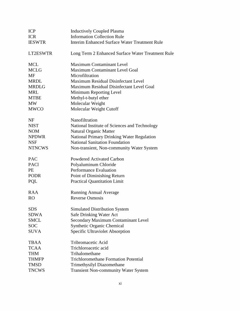
xi

ICP Inductively Coupled PlasmaICR Information Collection RuleIESWTR Interim Enhanced Surface Water Treatment Rule

LT2ESWTR Long Term 2 Enhanced Surface Water Treatment Rule

MCL Maximum Contaminant LevelMCLG Maximum Contaminant Level GoalMF MicrofiltrationMRDL Maximum Residual Disinfectant LevelMRDLG Maximum Residual Disinfectant Level GoalMRL Minimum Reporting LevelMTBE Methyl-t-butyl etherMW Molecular WeightMWCO Molecular Weight Cutoff

NF NanofiltrationNIST National Institute of Sciences and TechnologyNOM Natural Organic MatterNPDWR National Primary Drinking Water RegulationNSF National Sanitation FoundationNTNCWS Non-transient, Non-community Water System

PAC Powdered Activated CarbonPACl Polyaluminum ChloridePE Performance EvaluationPODR Point of Diminishing ReturnPQL Practical Quantitation Limit

RAA Running Annual AverageRO Reverse Osmosis

SDS Simulated Distribution SystemSDWA Safe Drinking Water ActSMCL Secondary Maximum Contaminant LevelSOC Synthetic Organic ChemicalSUVA Specific Ultraviolet Absorption

TBAA Tribromacetic AcidTCAA Trichloroacetic acidTHM TrihalomethaneTHMFP Trichloromethane Formation PotentialTMSD Trimethysilyl DiazomethaneTNCWS Transient Non-community Water System

xii

TOC Total Organic CarbonTOX Total Organic HalidesTOXFP Total Organic Halides Formation PotentialTTHM Total Trihalomethanes

UF UltrafiltrationUFC Uniform Formation ConditionUV UltravioletUV-254 Ultraviolet absorbance at a wavelength of 254 nm

WIDB Water Industry Data Base

ES-1

EXECUTIVE SUMMARY

BACKGROUND

The 1986 Amendments to the Safe Drinking Water Act (SDWA) required the United

States Environmental Protection Agency (EPA) to set maximum contaminant level goals

(MCLGs) for many contaminants found in drinking water. These MCLGs must provide an

adequate margin of safety from contaminant concentrations that are known or anticipated to

induce adverse effects on human health. For each contaminant, EPA must establish either

a treatment technique or a maximum contaminant level (MCL) that is as close to the MCLG

as is feasible with the use of best available technology (BAT).

Acting on the 1986 Amendments, EPA developed a list of disinfectants and

disinfection byproducts (DBPs) for possible regulation after several rounds of stakeholder

comments. The course of the Disinfection Byproduct Rule (DBPR) was decided by a

regulatory negotiation which took place among stakeholders in 1992-93. Following the

negotiation, EPA proposed three regulations: the Stage 1 DBPR, the Interim Enhanced

Surface Water Treatment Rule (IESWTR), and the Information Collection Rule (ICR). The

1994 proposed DBPR includes MCLs for selected DBPs and maximum residual disinfectant

levels (MRDLs) for selected disinfectants. Stage 1 of the DBPR, promulgated December 16,

1998, includes MCLs for trihalomethanes, haloacetic acids, bromate, and chlorite. MRDLs

were also finalized for chlorine, chloramines, and chlorine dioxide. The ICR, finalized in

May 1996, will provide occurrence data for DBPs and precursors, microbials, water quality

parameters, and treatment plant parameters. These data, along with the ICR treatment

studies, health effects research, and other research projects, will be used to develop the Stage

2 DBPR and the Long Term 2 Enhanced Surface Water Treatment Rule (LT2ESWTR). The

Stage 2 DBPR will be promulgated in 2002.

The MCLs and MRDLs will provide protection against the potential adverse health

effects associated with disinfectants and DBPs. During the regulatory negotiation process,

however, it was realized that these limits alone may not address the potential health risks

from all DBPs, including those which have yet to be identified. Consequently, a treatment

ES-2

technique requirement is included in the DBPR to remove natural organic matter (NOM),

which serves as a primary precursor for DBP formation.

The goal of the treatment technique is to provide additional removal of NOM, as

measured by total organic carbon (TOC). The treatment technique applies to Subpart H

systems (systems using surface water or groundwater under the direct influence of surface

water) that practice conventional coagulation or softening treatment. This Guidance Manual

defines the treatment technique for the DBPR and provides implementation assistance for

affected systems.

Subsequent to the completion of the reg-neg process, the 1996 Amendments to

SDWA were passed by Congress. Under these Amendments, EPA was required to expedite

the rule-making process for microbiological contaminants and DBPs. Consequently, EPA

promulgated the Stage 1 DBPR in December 1998. EPA negotiated an agreement in

principle under the auspices of the Federal Advisory Committee Act (FACA) to review the

1994 DBPR proposal and to modify its requirements based upon additional data and

information generated since the proposal. This information is discussed in the November 3,

1997 Federal Register (62 FR 59388). Some requirements were modified based upon

significant experience and study performed by utilities, universities, consultants and the

American Water Works Association (AWWA). This document reflects these modifications.

ENHANCED COAGULATION/ENHANCED SOFTENING DEFINITIONS

The purpose of the treatment technique for DBP precursor removal is to reduce the

formation of DBPs. NOM reacts with disinfectants to form DBPs; therefore, lowering the

concentration of NOM (as measured by TOC) can reduce DBP formation.

“Enhanced coagulation” is the term used to define the process of obtaining improved

removal of DBP precursors by conventional treatment. “Enhanced softening” refers to the

process of obtaining improved removal of DBP precursors by precipitative softening.

ES-3

Because TOC is easily measured and monitored, the treatment technique uses a TOC

removal requirement. However, basing a performance standard on a uniform TOC removal

requirement is inappropriate because some waters are especially difficult to treat. If the

TOC removal requirements were based solely upon the treatability of "difficult-to-treat"

waters, many systems with "easier-to-treat" waters would not be required to achieve

significant TOC removal. Alternatively, a standard based upon what many systems could

not readily achieve would introduce large transactional costs to States and utilities.

To address these concerns, a two-step standard for enhanced coagulation and

enhanced precipitative softening was developed. Step 1 includes TOC removal performance

criteria which, if achieved, define compliance. The Step 1 TOC removal percentages are

dependent on alkalinity, as TOC removal is generally more difficult in higher alkalinity

waters, and source water with low TOC levels. Step 2 allows systems with difficult-to-treat

waters to demonstrate to the State, through a specific protocol, an alternative TOC removal

level for defining compliance. The final rule also contains certain alternative compliance

criteria that allow a system to demonstrate compliance.

TESTING PROTOCOLS AND LABORATORY PROCEDURES

Initially, a utility should determine if it is required to implement the treatment

technique. If it is, it should evaluate full-scale TOC removal. If this evaluation shows that

the plant is not meeting the required TOC removal, some adjustment to the full-scale

coagulation or softening process will be needed. Before enhanced coagulation or enhanced

softening is implemented at full-scale, careful development of an implementation strategy,

adequate planning, and bench-, pilot-, and/or demonstration-scale (i.e. partial system) testing

should be performed. A system may also wish to evaluate whether any alternative

compliance criteria can be met.

Bench- and pilot-scale testing allow a utility to determine the TOC removal capability

of the plant for different treatment situations, determine the necessary adjustments to full-

scale operation, and, in some cases, to set an alternative percent TOC removal to comply

with the regulation under the Step 2 procedure. These tests are important and call for a well-

ES-4

defined testing protocol and strict laboratory procedures. The testing protocols for the Step

2 enhanced coagulation bench- and pilot-scale tests are presented in this document.

Laboratory testing methods are also given.

The evaluation of data collected as part of bench- and pilot-scale tests is an important

step in the process of full-scale implementation. To assist utilities in this analysis, data

analysis protocols are presented here. In addition, a number of example analyses are

provided to guide utilities through the evaluation process. Once these evaluations have been

performed, full-scale implementation can be conducted. Utilities should take precautions to

minimize any detrimental side effects of enhanced coagulation or enhanced softening. Items

such as secondary treatment impacts and customer water quality expectations need to be

considered. Suggestions to help minimize these effects are also presented in this document.

SECONDARY EFFECTS

The implementation of enhanced coagulation or enhanced softening can involve

process modifications and can be accompanied by secondary impacts or side effects. Some

side effects will be beneficial to the treatment process while others may be detrimental. This

guidance manual identifies and characterizes the major secondary impacts utilities may

encounter and provides possible mitigation strategies. These impacts include the effect of

enhanced coagulation/enhanced softening on the following:

& Inorganic constituents levels (manganese, aluminum, sulfate, chloride, and sodium)

& Corrosion control

& Disinfection

& Particle and pathogen removal

& Residuals (handling, treatment, disposal)

& Operation and maintenance

& Recycle streams

Not all utilities will experience secondary impacts. Some utilities may experience

very minor secondary effects while others may experience more substantial effects. All

ES-5

utilities required to practice enhanced coagulation and enhanced softening, however, should

be aware of the potential effects implementation of enhanced coagulation and softening may

have on plant operation.

OTHER EPA GUIDANCE MANUALS

This manual is one in a series of guidance manuals published by EPA to assist both

States and public water systems in complying with the IESWTR and Stage 1 DBPR drinking

water regulations. Other EPA guidance manuals scheduled to be released in the Spring of

1999 include:

& Disinfection Profiling and Benchmarking Guidance Manual

& Alternative Disinfectants and Oxidants Guidance Manual

& Microbial and Disinfection Byproduct Simultaneous Compliance Guidance Manual

& Uncovered Finished Water Reservoirs Guidance Manual

& Guidance Manual for Compliance with the Interim Enhanced Surface WaterTreatment Rule: Turbidity Provisions

& Sanitary Surveys Guidance Manual

& Unfiltered Systems Guidance Manual

Chapter 1

DISINFECTION BYPRODUCT RULE OVERVIEW

Table of Contents

Page

1.0 DISINFECTION BYPRODUCT RULE OVERVIEW1.1 Introduction. . . . . . . . . . . . . . . . . . . . . . . . . . . . . . . . . . . . . . . . . . . . . . 1-11.2 General Requirements . . . . . . . . . . . . . . . . . . . . . . . . . . . . . . . . . . . . . . 1-1

1.2.1 Treatment Technique. . . . . . . . . . . . . . . . . . . . . . . . . . . . . . . . . 1-11.2.2 Compliance Schedule. . . . . . . . . . . . . . . . . . . . . . . . . . . . . . . . 1-21.2.3 Maximum Contaminant Levels. . . . . . . . . . . . . . . . . . . . . . . . . 1-31.2.4 Maximum Residual Disinfectant Levels. . . . . . . . . . . . . . . . . . 1-5

1.3 Analytical Requirements . . . . . . . . . . . . . . . . . . . . . . . . . . . . . . . . . . . . 1-61.4 Reporting Requirements . . . . . . . . . . . . . . . . . . . . . . . . . . . . . . . . . . . . 1-61.5 Compliance . . . . . . . . . . . . . . . . . . . . . . . . . . . . . . . . . . . . . . . . . . . . . . 1-6

List of Tables

1-1 Compliance Dates for the DBPR and ESWTR . . . . . . . . . . . . . . . . . . . . . . . . . 1-31-2 MCLGs for the Stage 1 DBPR . . . . . . . . . . . . . . . . . . . . . . . . . . . . . . . . . . . . . 1-41-3 MCLs for the Stage 1 DBPR . . . . . . . . . . . . . . . . . . . . . . . . . . . . . . . . . . . . . . . 1-41-4 MRDLGs for the DBPR . . . . . . . . . . . . . . . . . . . . . . . . . . . . . . . . . . . . . . . . . . 1-51-5 MRDLs for the DBPR . . . . . . . . . . . . . . . . . . . . . . . . . . . . . . . . . . . . . . . . . . . . 1-5

1-1

1.0 DISINFECTION BYPRODUCT RULE OVERVIEW

1.1 INTRODUCTION

The purpose of the Stage 1 Disinfection Byproduct Rule (DBPR) is to reduce

exposure to disinfection byproducts (DBPs) by limiting allowable DBP concentrations in

drinking water, and by removing DBP precursor material to reduce the formation of

identified and unidentified DBPs. Stage 1 of the DBPR establishes maximum contaminant

levels (MCLs) for some of the known DBPs, maximum residual disinfection levels

(MRDLs) for commonly used disinfectants, and a treatment technique for removal of DBP

precursor material to reduce the formation of DBPs. Microbial and chemical contaminant

data collected under the Information Collection Rule (ICR), as well as health effects and

treatment research, will be used in the development of the Long Term 2 Enhanced Surface

Water Treatment Rule (LT2ESWTR) and the Stage 2 DBPR. Negotiations for the

development of these rules began in December 1998 and will incorporate the additional

understanding of DBPs and the disinfection process developed from the ICR database.

1.2 GENERAL REQUIREMENTS

1.2.1 Treatment Technique

In addition to the MCLs and MRDLs, the DBPR requires the use of a treatment

technique to reduce DBP precursors and to minimize the formation of unknown DBPs.

This treatment technique is termed Enhanced Coagulation or Enhanced Precipitative

Softening. It requires that a specific percentage of influent total organic carbon (TOC) be

removed during treatment. The treatment technique uses TOC as a surrogate for natural

organic matter (NOM), the precursor material for DBPs. The treatment technique applies

to subpart H systems (plants using surface water or groundwater under the direct influence

of surface water) that practice conventional filtration treatment (including coagulation and

sedimentation) or softening treatment.

1-2

A TOC concentration of greater than 2.0 mg/L in a system's raw water is the trigger

for implementation of the treatment technique. Specific definitions and alternative

compliance criteria for the treatment technique requirement are presented in Chapter 2.

If a plant is required to practice enhanced coagulation, it must reduce the TOC in the

raw water by a specified percentage before the treated water TOC sampling point, which can

be no later than the combined filter effluent turbidity monitoring location. The required

percent TOC reduction is based on the raw water TOC and alkalinity, and is defined as Step

1 of the treatment technique, as described in Chapter 2. Note that paired samples, one from

the raw water and one from the finished water, are taken simultaneously to determine

compliance. The raw water sample must be taken from untreated water, because the

application of oxidants or other treatment chemicals can change the nature of the TOC,

resulting in unrepresentative analytical results.

Both enhanced coagulation and enhanced softening plants may also use alternative

compliance criteria to demonstrate compliance with the treatment technique. If an enhanced

coagulation plant does not achieve the specified TOC removal as a running annual average,

or any of the alternative compliance criteria, it must proceed to Step 2 of the treatment

technique. For plants practicing enhanced coagulation, the Step 2 procedure requires jar

testing to set an alternative TOC percent removal for determining compliance. Enhanced

softening plants are not required to conduct jar or bench-scale testing. These and other

regulatory requirements are discussed in Chapter 2 of this guidance manual.

1.2.2 Compliance Schedule

The Stage 1 DBPR MCLs and MRDLs apply to community water systems (CWSs)

and non-transient, non-community water systems (NTNCWSs) that add a disinfectant to any

part of the treatment process, including residual disinfection. Table 1-1 summarizes a time

frame for proposed, final, and effective regulations for the Stage 1 DBPR and the IESWTR.

1-3

TABLE 1-1Compliance Dates for the DBPR and ESWTR

Rule(Promulgation Date)

Subpart HPublic Water Systems

Ground WaterPublic Water Systems

��10,000 <10,000 ��10,000 <10,000

DBPR Stage 1 (December 16, 1998)

12/011 12/03 12/01 12/01

IESWTR (December 16, 1998)

12/011 N/A N/A N/A

1. States may grant systems two additional years for compliance if capital improvements are necessary.

Because of potential acute health effects, the MRDL for chlorine dioxide also applies

to transient, non-community water systems (TNCWSs). The effective dates for this

regulation will be staggered based on system size and raw water sources as follows:

& CWSs and NTNCWSs: Subpart H systems serving 10,000 or more persons mustcomply with the rule’s provisions beginning December 2001. Subpart H systemsserving fewer than 10,000 persons and systems using only ground water not underthe direct influence of surface water must comply with this subpart beginningDecember 2003.

& TNCWSs: Subpart H systems serving 10,000 or more persons and using chlorinedioxide as a disinfectant or oxidant must comply with the chlorine dioxide MRDLbeginning December 2001. Subpart H systems serving fewer than 10,000 persons andusing chlorine dioxide as a disinfectant or oxidant, and systems using only groundwater not under the direct influence of surface water and using chlorine dioxide asa disinfectant or oxidant must comply with the chlorine dioxide MRDL beginningDecember 2003.

1.2.3 Maximum Contaminant Levels

Congress has given EPA broad authority to establish National Primary Drinking

Water Regulations (NPDWRs) and Maximum Contaminant Level Goals (MCLGs). The

MCLGs are developed as non-enforceable health goals. As defined in 40 CFR 141.2, the

MCLG is set "at the level at which no known or anticipated adverse effect on the health of

the person would occur, and which allows an adequate margin of safety." EPA policy is to

1-4

establish MCLGs for suspected human carcinogens at zero. MCLs are the legally

enforceable standard, and are set as close to the MCLGs as feasible, taking technology and

cost into account.

The DBPR establishes MCLs for the most common and well-studied halogenated

DBPs: total trihalomethanes (TTHMs) and five of the nine haloacetic acid species (HAA5),

as well as bromate and chlorite. TTHM is defined as the sum of chloroform, bromoform,

bromodichloromethane, and dibromochloromethane. HAA5 is defined as the sum of mono-

, di-, and trichloroacetic acids, and mono- and dibromoacetic acids. The MCLGs for the

DBPR are listed in Table 1-2. MCLs for the DBPR are shown in Table 1-3.

TABLE 1-2MCLGs for the Stage 1 DBPR

Bromoform 0 mg/L

Chloroform 0 mg/L

Bromodichloromethane 0 mg/L

Dibromochloromethane 0.06 mg/L

Dichloroacetic acid 0 mg/L

Trichloroacetic acid 0.3 mg/L

Bromate 0 mg/L

Chlorite 0.8 mg/L

TABLE 1-3MCLs for the Stage 1 DBPR

Total Trihalomethanes (TTHMs)* 0.080 mg/L

Haloacetic Acids (HAA5)* 0.060 mg/L

Bromate* 0.010 mg/L

Chlorite 1.0 mg/L* Compliance is based on a running annual average, computed quarterly

1-5

1.2.4 Maximum Residual Disinfectant Levels

Similar to MCLGs, maximum residual disinfectant level goals (MRDLGs) are health

goals and are not legally enforceable. The MRDLGs for the DBPR are shown in Table 1-4.

The DBPR also establishes maximum residual disinfectant levels (MRDLs) for the

most commonly used disinfectants, which are enforceable limits similar to MCLs. MRDLs

for the DBPR are shown in Table 1-5. The MRDLs for chlorine and chloramines, but not

chlorine dioxide, may be exceeded to protect public health from specific microbiological

contamination events. These exceedances would be for specific problems caused by

unusual conditions such as line breaks, cross-contamination events, or raw water

contamination.

TABLE 1-4MRDLGs for the DBPR

Chlorine (as Cl2) 4 mg/L

Chloramine (as Cl2) 4 mg/L

Chlorine dioxide (as ClO2) 0.8 mg/L

TABLE 1-5MRDLs for the DBPR

Chlorine (as Cl2)* 4.0 mg/L

Chloramine (as Cl2)* 4.0 mg/L

Chlorine Dioxide (as ClO2) 0.8 mg/L

* Compliance is based on a running annual average, computed quarterly

1-6

1.3 ANALYTICAL REQUIREMENTS

Plants must use only the analytical methods specified in the regulation for monitoring

purposes. Approved analytical methods are outlined in Chapter 5.

1.4 REPORTING REQUIREMENTS

Plants are required to report their monitoring results to the State primacy agency

within ten days after the end of each monitoring quarter in which the samples were

collected. Plants required to sample less frequently than quarterly must report to the State

within ten days after the end of the monitoring period in which the samples were collected.

Monitoring and reporting requirements for the treatment technique are explained in Chapter

4 of this guidance manual.

1.5 COMPLIANCE

TTHM, HAA5, and Bromate

Compliance with the MCLs for TTHM and HAA5 and with the MRDLs for chlorine

and chloramine is based on a running annual average, computed using quarterly samples.

Compliance with the MCL for bromate is based on a running annual average of monthly

samples, computed quarterly, or monthly averages if the system takes more than one sample

in a month.

Chlorite

Compliance with the MRDL for chlorite and chlorine dioxide is more complex as a

result of potential acute health effects. Plants that use chlorine dioxide for disinfection or

oxidation must conduct monitoring for chlorite and chlorine dioxide. Routine chlorite

monitoring requires analyzing one sample per day at the entrance to the distribution system,

as well as taking a three-sample set once per month from within the distribution system.

The distribution system sampling must consist of one sample from each of the following

1-7

locations: near the first customer, at a location representative of average residence time, and

at a location reflecting maximum residence time in the distribution system.

Additional chlorite sampling also must be conducted in this manner. For any day

when the daily chlorite sample exceeds 1.0 mg/L, the plant must take a three-sample set

from within the distribution system on the following day, at the locations prescribed for

monthly monitoring. Compliance with the chlorite MCL is based on the arithmetic average

of any three-sample set taken as required in the distribution system.

Chlorine Dioxide

Routine chlorine dioxide monitoring requires taking one sample per day at the

entrance to the distribution system. In addition, for any daily sample that exceeds 0.8 mg/L,

the plant must take three chlorine dioxide samples in the distribution system on the

following day, located as follows: (1) If there are no disinfection addition points after the

entrance to the distribution system (i.e., no booster chlorination), the plant must take three

samples as close to the first customer as possible, at intervals of at least six hours. (2) If

there are disinfection addition points after the entrance to the distribution system, the plant

must take one sample at each of the following locations: as close to the first customer as

possible, in a location representative of average residence time, and as close to the end of

the distribution system as possible (reflecting maximum residence time in the distribution

system).

Violations of the chlorine dioxide MRDL can be either acute or non-acute. If any

daily sample taken at the entrance to the distribution system exceeds the MRDL, and on the

following day one (or more) of the three samples taken in the distribution system exceeds

the MRDL, the plant is in violation of the MRDL and must notify the public pursuant to the

procedures for acute health risks. If any two consecutive daily samples taken at the entrance

to the distribution system exceed the MRDL and all distribution system samples taken are

below the MRDL, the plant is in violation of the MRDL and must notify the public pursuant

to the procedures for non-acute health risks.

Compliance with the treatment technique for TOC removal is based on a running

annual average, which in turn is based on the quarterly average of monthly samples.

1-8

Compliance calculations, monitoring, and reporting for the treatment technique are

discussed in Chapter 4. The Implementation Guidance Manual for the IESWTR and Stage

1 DBPR (1999) contains a detailed discussion of monitoring and reporting requirements,

and requirements for data submittal to the States.

Chapter 2

DEFINITIONS OF ENHANCED COAGULATION ANDENHANCED PRECIPITATIVE SOFTENING

Table of Contents

Page

2.0 DEFINITIONS OF ENHANCED COAGULATION AND ENHANCED PRECIPITATIVE SOFTENING2.1 Introduction. . . . . . . . . . . . . . . . . . . . . . . . . . . . . . . . . . . . . . . . . . . . . . . . . . 2-12.2 Applicability of Treatment Technique Requirements. . . . . . . . . . . . . . . . . . 2-22.3 TOC Removal Performance Requirements. . . . . . . . . . . . . . . . . . . . . . . . . . 2-2

2.3.1 Step 1 TOC Removal Requirements. . . . . . . . . . . . . . . . . . . . . . . . . 2-32.3.2 Step 2 Alternative TOC Removal Requirements. . . . . . . . . . . . . . . 2-62.3.3 Frequency of Step 2 Testing. . . . . . . . . . . . . . . . . . . . . . . . . . . . . . . 2-8

2.4 Alternative Compliance Criteria . . . . . . . . . . . . . . . . . . . . . . . . . . . . . . . . . . 2-82.4.1 Finished Water SUVA Jar Testing. . . . . . . . . . . . . . . . . . . . . . . . . 2-10

2.5 Treatment Technique Waiver . . . . . . . . . . . . . . . . . . . . . . . . . . . . . . . . . . . 2-112.6 Sampling Frequency for Compliance Calculations. . . . . . . . . . . . . . . . . . . 2-112.7 Compliance Considerations When Blending Source Waters. . . . . . . . . . . 2-12

List of Tables

2-1 Required Removal of TOC by Enhanced Coagulation for Plants UsingConventional Treatment: Step 1 Removal Percentages. . . . . . . . . . . . . . . . . . . . . 2-5

2-2 Target pH Under Step 2 Requirements . . . . . . . . . . . . . . . . . . . . . . . . . . . . . . . . . 2-72-3 Treatment Technique Compliance Schedule . . . . . . . . . . . . . . . . . . . . . . . . . . . . . 2-8

List of Figures

2-1 Guidelines for Achieving Compliance with Enhanced Coagulation/Enhanced Softening Criteria . . . . . . . . . . . . . . . . . . . . . . . . . . . . . . . . . . . . . . . . . 2-4

2-1

2.0 DEFINITIONS OF ENHANCED COAGULATIONAND ENHANCED PRECIPITATIVE SOFTENING

2.1 INTRODUCTION

The term "enhanced coagulation” refers to the process of improving the removal of

disinfection byproduct (DBP) precursors in a conventional water treatment plant. “Enhanced

softening” refers to the improved removal of DBP precursors by precipitative softening.

The removal of natural organic matter (NOM) in conventional water treatment processes

by the addition of coagulant has been demonstrated by laboratory research and by pilot-,

demonstration-, and full-scale studies. Several researchers have shown that total organic carbon

(TOC) in water, used as an indicator of NOM, exhibits a wide range of responses to treatment

with aluminum and iron salts (Chowdhury et al., 1997; Edwards et al., 1997; White et al., 1997;

Owen et al., 1996; Krasner and Amy, 1995; Owen et al., 1993; James M. Montgomery, 1992;

Hubel and Edzwald, 1987; Knocke et al., 1986; Chadik and Amy, 1983; Semmens and Field,

1980; Young and Singer, 1979; Kavanaugh, 1978). The majority of these studies have been

conducted using regular and reagent grade alum (Al2[SO4]3.14H2O and Al2[SO4]3

.18H2O,

respectively) as the coagulant, but iron salts also have been shown to be effective for removing

TOC from water. Polyaluminum chloride (PACl) and cationic polymers also can be effective for

removing TOC. Cationic polymers (as well as anionic and non-ionic polymers) have proven to

be valuable in creating settleable floc when high dosages of aluminum or iron salts are used.

Specific organic polymers have been shown to remove color in water treatment applications, but

significant TOC removal by organic polymers in conventional facilities has not been

demonstrated, and organic polymers may actually increase the TOC level of the water

(AWWARF, 1989).

The intent of the treatment technique discussed in this document is to establish TOC

removal requirements based on enhanced coagulation/precipitative softening so that:

& significant TOC reductions can be achieved without the addition of unreasonableamounts of coagulant; and

& regulatory criteria can easily be enforced with minimal State transactional costs.

2-2

To achieve these objectives, a TOC-based performance standard has been developed for

enhanced coagulation and enhanced precipitative softening using a 2-step system. Step 1 requires

removal of a specific percentage of influent TOC to demonstrate compliance, based on the TOC

and alkalinity of the source water. Step 2 requires enhanced coagulation systems that cannot meet

the Step 1 criteria or the alternative compliance criteria to establish an alternative TOC removal

percentage for defining compliance. These steps are described in detail in Section 2.3. Enhanced

softening systems are expected to meet either the Step 1 removal requirements or one of the

alternative compliance criteria. Therefore, EPA has not developed a Step 2 procedure for systems

using enhanced softening.

2.2 APPLICABILITY OF TREATMENT TECHNIQUE REQUIREMENTS

Public water utilities must implement enhanced coagulation or enhanced softening to

achieve percent TOC removal levels specified in Section 2.3.1 if:

& the source water is surface water or ground water under the direct influence of surfacewater (Subpart H systems); and

& the utility uses conventional treatment (i.e., flocculation, coagulation or precipitativesoftening, sedimentation, and filtration).

Some types of treatment trains (e.g., direct filtration systems, diatomaceous earth filtration

systems, slow sand filtration) and ground water systems are excluded from the enhanced

coagulation/enhanced softening requirements because: (1) their source waters are generally

expected to be of a higher quality (have lower TOC levels) than waters treated by conventional

water treatment plants; and (2) the treatment trains are not typically configured to allow

significant TOC removal (i.e., they lack sedimentation basins to settle out TOC).

2.3 TOC REMOVAL PERFORMANCE REQUIREMENTS

Individual treatment plants are required to achieve a specified percent removal (Step 1)

of influent TOC between the raw water sampling point and the treated water TOC monitoring

2-3

location (no later than the combined filter effluent turbidity monitoring location). Compliance

with the TOC removal requirement is based on a running annual average, computed quarterly.

Plants, therefore, will make four compliance determinations each year, one per quarter, based on

the most recent four quarters of data. If a plant practicing enhanced coagulation achieves a

running annual average removal ratio of less than 1.0 (the ratio of actual percent TOC removal

to required percent TOC removal) after the first year of TOC compliance monitoring and it does

not meet any alternative compliance criteria, it is required to perform jar or pilot-scale testing

(Step 2 testing) to set an alternative TOC removal requirement, and report the results of testing

to the State within three months of failing to achieve a running annual average removal ratio of

greater than or equal to 1.0. The alternative removal percentage is subject to State approval. The

compliance process is illustrated in Figure 2-1.

Enhanced softening plants unable to meet the Step 1 TOC removal percentage on a

running annual average basis can also establish compliance by achieving either of two softening-

specific alternative compliance criteria. These two criteria are summarized in Section 2.4.2.

Enhanced softening plants are not required to perform Step 2 testing to set an alternative TOC

removal percentage.

2.3.1 Step 1 TOC Removal Requirements

Table 2-1 summarizes the percent TOC removal requirements for enhanced coagulation.

Enhanced softening plants are required to comply with the TOC removal percentages in the far

right column of Table 2-1 (i.e., where alkalinity >120 mg/L as CaCO3 ). The percent TOC

removals identified in this table are based upon a large database of bench-, pilot-, and full-scale

studies at a large number of utilities across the nation (Chowdhury et al., 1997).

The TOC removal criteria presented in Table 2-1 were selected so that a large majority

(e.g., 90 percent) of plants required to operate with enhanced coagulation or enhanced softening

will be able to meet the TOC removal percentages. Setting the removal criteria this way is

expected to result in: (1) smaller transactional costs to the State because fewer evaluations of Step

2 experimental data will be required; and (2) reasonable increases in coagulant doses at affected

plants.

2-4

G ather da ta on raw and trea ted w ater to com pare w ith the com pliance c rite r ia

Q ualifyfo r any

a lte rnative com pliancecrite ria (see

Sec 2 .4)

Is fu ll-sca le T O C

rem ova l � requ iredT O C rem ova l? (see

T ab le 2 -1 Sec . 2 .3 .1 )

In com pliance w ith requ irem entsY es

N o

E va luate fu ll-sca le capab ility to com ply w ith requ ired T O C rem ova l

N o

C ansystem ach ieve

requ ired T O C rem oval a t fu ll sca le?

(see Sec.2 .3 .2 )

C ansystem ach ieve

requ ired T O C rem oval a t fu ll sca le?

(see Sec.2 .3 .2 )

Perfo rm ja r tests toestab lish a lte rnative

T O C rem ova l percentage(N ot app licab le toso ften ing p lan ts)

Perfo rm ja r tests toestab lish a lte rnative

T O C rem ova l percentage(N ot app licab le toso ften ing p lan ts)

D eve lop stra tegy toim p lem ent enhancedcoagu la tion /enhancedsoften ing a t fu ll scale

D eve lop stra tegy toim p lem ent enhancedcoagu la tion /enhancedsoften ing a t fu ll scale

A pp ly to S ta te forapprova l o f a lte rna tiveT O C rem ova l c r ite r ia

(see Sec.2 .5 re . w a iver)

A pp ly to S ta te forapprova l o f a lte rna tiveT O C rem ova l c r ite r ia

(see Sec.2 .5 re . w a iver)

S ta te D en ies

N o Y es

Sta te

A pprovesC onduct p ilo t-sca le or dem onstra tion-scale tests

to consider secondary e ffec ts (see C hapter 6 )

C onduct p ilo t-sca le or dem onstra tion-scale teststo consider secondary e ffec ts (see C hapter 6 )

Im p lem ent enhanced coagu la tion /enhanced so ften ing a t fu ll scale

Im plem ent enhanced coagu la tion /enhanced so ften ing a t fu ll scale

T O C rem ova l � requ ired T O C

rem ova l?

T O C rem ova l � requ ired T O C

rem ova l?

Y es

N o

Y es

S T E P 1

S T E P 2F or E nhanced C oagu la t ion

P lan ts O n ly

F igu re 2-1. G u ide lines fo r A ch iev ingC om pliance w ith E nhanced C oagu la tion /E nhanced Soften ing C riteria

(A ll So ften ing P lan tsF o llow R igh t S ide

of D iagram )

Figure 2-1. Guidelines for Achieving Compliance with Enhanced Coagulation/enhanced

Softening Criteria

2-5

TABLE 2-1

Required Removal of TOC by Enhanced CoagulationFor Plants Using Conventional Treatment:

Step 1 Removal Percentagesa, b

SOURCE

WATER

TOC (mg/L)

SOURCE WATER ALKALINITY (mg/L as CaCO 3)

0 to 60 >60 to 120 >120c

>2.0 - 4.0 35.0% 25.0% 15.0%

>4.0 - 8.0 45.0% 35.0% 25.0%

>8.0 50.0% 40.0% 30.0%Notes:

a. Enhanced coagulation and enhanced softening plants meeting at least one of the six alternative compliance criteria inSection 2.4 are not required to meet the removal percentages in this table.

b. Softening plants meeting one of the two alternative compliance criteria for softening in Section 2.4 are not required tomeet the removal percentages in this table.

c. Plants practicing precipitative softening must meet the TOC removal requirements in this column.

The percent removal requirements specified in Table 2-1 were developed with recognition

of the tendency for TOC removal to become more difficult as alkalinity increases and TOC

decreases. In higher alkalinity waters, pH depression to a level at which TOC removal is optimal

(e.g., pH between 5.5 and 6.5) is more difficult and cannot be achieved easily through the addition

of coagulant alone. Compliance with the TOC removal requirements is calculated with a running

annual average, computed quarterly. Month to month changes in source water TOC and/or

alkalinity levels will cause some plants to move from one box of Table 2-1 to another. The

required TOC removal, therefore, may change month to month based on the TOC and alkalinity

level of the monthly source water compliance sample. See Chapter 4 for example compliance

calculations that address this possibility.

Plants not currently in compliance with the values in Table 2-1 may wish to perform jar

testing to evaluate modifications to coagulant dose and/or pH conditions to determine whether

the required TOC removals can be achieved. If the TOC removal performance criteria identified

in Table 2-1 cannot be met, enhanced coagulation systems must implement the Step 2

requirements discussed below.

2-6

2.3.2 Step 2 Alternative TOC Removal Requirements

Some plants required to implement enhanced coagulation will not achieve the removals

in Table 2-1 because of unique water quality characteristics. These plants are required to conduct

jar or bench scale testing under the Step 2 procedure to establish an alternative TOC removal

requirement.

The purpose of the jar tests is to establish an alternative TOC removal requirement,

not to determine full-scale operating conditions. Once an alternative removal requirement is

defined by bench- or pilot-scale testing and approved by the State, the utility is free to achieve that

removal in the full-scale plant with any combination of coagulant, coagulant aid, filter aid, and

acid addition. Plants may wish to perform further jar and pilot testing before implementing full-

scale changes. The National Sanitation Foundation has established maximum limits for the

addition of some treatment chemicals; these limits are summarized in Section 7.3.1. Utilities

required to implement the Step 2 requirements should follow the procedures described in Chapter

3.

Under the Step 2 procedure, 10 mg/L increments of alum (or an equivalent amount of

ferric salt) are added, without acid addition for pH adjustment, to determine the incremental

removal of TOC. The Step 2 procedure can be performed through either batch (bench-scale) or

continuous flow (pilot- or full-scale) testing. TOC removal is calculated for each 10 mg/L

increment of regular-grade alum or equivalent amount of iron salt added during jar testing.

Coagulant must be added in the required increments until the target pH shown in Table 2-2 is

achieved. The point of diminishing return (PODR) for coagulant addition is defined as the point

on the TOC removal vs. coagulant addition plot where the slope changes from greater than 0.3/10

to less than 0.3/10, and remains less than 0.3/10 until the target pH is reached. The percent TOC

removal achieved at the PODR is defined, per approval by the State, as the alternative

percent TOC removal requirement.

2-7

TABLE 2-2

Target pH Under Step 2 Requirements

ALKALINITY

(mg/L as CaCO3)

TARGET pH

0 - 60 5.5

> 60 - 120 6.3

> 120 - 240 7.0

> 240 7.5

The Step 2 procedure requires that incremental coagulant addition be continued until the

pH of the tested sample is at or below the “target pH” (Table 2-2) to ensure that the treatability

of the sample is examined over a range of pH values (see Chapter 3 for details). The target pH

values are dependent upon the alkalinity of the raw water to account for the fact that higher

coagulant dosages are needed to reduce pH in higher alkalinity waters. The regulation requires

that waters with alkalinities of less than 60 mg/L (as CaCO3), for which addition of small amounts

of coagulant drives the pH below the target pH before significant TOC removal is achieved, add

necessary chemicals to maintain the pH between 5.3 and 5.7 until the PODR criterion is met. The

chemical used to adjust the pH should be the same chemical used in the full-scale plant, unless

that chemical does not perform adequately in jar tests. Substitute chemicals should be used in this

case. A bench-scale method for determining the PODR and alternative TOC removal requirement

under the Step 2 procedure is described in Section 3.2.2.

Compliance with the TOC removal requirements is based on a running annual average;

therefore, systems need 12 months of TOC monitoring data to make a compliance determination.

Since Step 2 bench- or pilot-scale testing is only required when a system fails to achieve a

running annual average removal ratio greater than or equal to 1.0 (i.e., the system is out of

compliance), Step 2 testing will not be performed until the second year of TOC compliance

sampling. If the State approves the Step 2 TOC removal percentage, the State may make that

percentage retroactive for determining compliance. The schedule for compliance with the

treatment technique is shown in Table 2-3.

2-8

TABLE 2-3

Treatment Technique Compliance Schedule

COMPLIANCE ACTION

POPULATION SERVED

�10,000 <10,000

1. Begin TOC compliance monitoring January 20021 January 20041

2. Calculate first Running Annual Average (RAA) for TOC removal compliance

January 2003 January 2005

3. Plants with RAA < 1.0 submit results of Step 2 testing to State

February throughApril 2003

February throughApril 2005

Note: 1 EPA recommends that systems begin at least one year earlier to determine whether compliance can be achieved.

2.3.3 Frequency of Step 2 Testing

States may wish to have plants perform Step 2 jar testing at least once per quarter for the

first year after treatment technique implementation to examine seasonal changes in treatability.

The State can consider the variability and characteristics of source waters to detemine site-specific

Step 2 testing frequency. An alternative TOC removal percentage set with the Step 2 procedure

remains in effect until the State approves a new value based on the results of new Step 2 testing.

2.4 ALTERNATIVE COMPLIANCE CRITERIA

Certain waters are less amenable to effective removal of TOC by coagulation or

precipitative softening. For this reason, alternative compliance criteria have been developed to

allow plants flexibility for establishing compliance with the treatment technique requirements.

These criteria recognize the low potential of certain waters to produce DBPs, and also account

for those waters not amenable to good TOC removal that may not meet the Step 1 TOC removal

requirement.

A plant can establish compliance with the enhanced coagulation or enhanced softening

TOC removal requirement if any one of the following six alternative compliance criteria is met:

1. Source water TOC <2.0 mg/L: If the source water contains less than 2.0 mg/L of TOC,calculated quarterly as a running annual average, the utility is in compliance with the

2-9

treatment technique. This criterion also can be used on a monthly basis, i.e., forindividual months in which raw water TOC is less than 2.0 mg/L, the plant can establishcompliance for that month by meeting this criterion.

2. Treated water TOC <2.0 mg/L: If a treated water contains less than 2.0 mg/L TOC,calculated quarterly as a running annual average, the utility is in compliance with thetreatment technique. This criterion also can be used on a monthly basis, i.e., forindividual months in which treated water TOC is less than 2.0 mg/L, the plant canestablish compliance for that month by meeting this criterion. Treated water TOCsampling is conducted no later than combined filter effluent turbidity monitoring.

3. Raw water SUVA �2.0 L/mg-m: If the raw water specific ultraviolet absorption (SUVA)is less than or equal to 2.0 L/mg-m, calculated quarterly as a running annual average, theutility is in compliance with the treatment technique requirements. This criterion is alsoavailable on a monthly basis, i.e., for individual months in which raw water SUVA is lessthan or equal to 2.0 L/mg-m, the plant can establish compliance for that month by meetingthis criterion. See section 5.2.4 for a discussion of SUVA.

4. Treated Water SUVA �2.0 L/mg-m: If the treated water SUVA is less than or equal to2.0 L/mg-m, calculated quarterly as a running annual average, the utility is in compliancewith the treatment technique requirements. This criterion is also available on a monthlybasis, i.e., for individual months in which treated water SUVA is less than or equal to 2.0L/mg-m, the plant can establish compliance for that month by meeting this criterion. SeeSection 5.2.4 for a discussion of SUVA. Treated water SUVA sampling is to beconducted no later than combined filter effluent turbidity monitoring.

5. Raw Water TOC <4.0 mg/L; Raw Water Alkalinity >60 mg/L (as CaCO3); TTHM <40µg/L; HAA5 <30 µg/L: It is more difficult to remove appreciable amounts of TOC fromwaters with higher alkalinity and lower TOC levels. Therefore, utilities that meet theabove criteria can establish compliance with the treatment technique requirements. Allof the parameters (e.g., TOC, alkalinity, TTHM, HAA5) are based on running annualaverages, computed quarterly. TTHM and HAA5 compliance samples are used to qualifyfor this alternative performance criterion.

Additionally, utilities that have made a clear and irrevocable financial commitment (priorto the utility’s effective compliance date for the DBPR) to technologies that will limitTTHM and HAA5 to 40 µg/L and 30 µg/L respectively, do not have to practice enhancedcoagulation if the TOC and alkalinity levels of this criterion also are met.

6. TTHM <40 µg/L and HAA5 <30 µg/L with only chlorine for disinfection: Plants that useonly free chlorine as their primary disinfectant and for maintenance of a residual in thedistribution system, and achieve the stated TTHM and HAA5 levels, are in compliancewith the treatment technique. The TTHM and HAA5 levels are based on running annual

2-10

averages, computed quarterly. TTHM and HAA5 compliance samples are used to qualifyfor this alternative performance criterion.

Example compliance calculations using these alternative compliance criteria are included

in Chapter 4.

Softening plants may demonstrate compliance if they meet any of the six alternative

compliance criteria listed above or one of the two alternative compliance criteria listed below:

1. Softening that results in lowering the treated water alkalinity to less than 60 mg/L (asCaCO3), measured monthly and calculated quarterly as a running annual average.

2. Softening that results in removing at least 10 mg/L of magnesium hardness (as CaCO3),measured monthly and calculated quarterly as a running annual average.

Softening plants that currently practice lime softening are not required to change to lime-

soda ash softening by the enhanced softening treatment technique.

If a utility takes more than one compliance sample any month to demonstrate compliance

with an alternative compliance criterion, the results of those samples should be averaged to

determine whether the alternative compliance criterion has been met.

2.4.1 Finished Water SUVA Jar Testing

Specific ultraviolet absorption (SUVA) is an indicator of the humic content of water. It

is a calculated parameter equal to the ultraviolet (UV) absorption at a wavelength of 254 nm

divided by the dissolved organic carbon (DOC) content of the water (in mg/L). The principle

behind this measurement is that UV-absorbing constituents will absorb UV light in proportion

to their concentration. Waters with low SUVA values contain primarily non-humic organic

matter and are not amenable to enhanced coagulation. On the other hand, waters with high SUVA

values generally are amenable to enhanced coagulation.

A treated water SUVA criterion may allow some utilities to determine compliance with

the treatment technique if the SUVA value is less than 2.0 L/mg-m. The determination of SUVA

should be made on finished water that has not been exposed to any oxidant during treatment. If

there is no oxidant (such as chlorine) added prior to the finished water TOC and UV-254

monitoring, full-scale samples can be used to calculate SUVA to allow comparison with this

criterion. However, if oxidants are added prior to the finished water TOC and UV-254

2-11

monitoring, the utilities are required to establish treated water SUVA by conducting a jar test in

which no disinfectants are added. The jar test can be performed by adding an equivalent amount

of coagulant (metal coagulant plus any polymer that is used in full-scale) in a jar test apparatus

and performing bench-scale coagulation tests. Details on jar testing are presented in Section 3.2.

After completion of the jar test, the settled water should be characterized for its DOC

and UV-254 parameters to calculate SUVA. (Filtration with a pre-washed 0.45 )m membrane

is required for DOC and UV-254 determination). Due to interference from iron in the UV-254

measurement, utilities using ferric salts for coagulation are required to conduct the jar test

described above using equivalent amounts of alum.

2.5 TREATMENT TECHNIQUE WAIVER

Plants that consistently fail to achieve the PODR (i.e., the slope of the TOC vs. coagulant

dose curve is never greater than 0.3 mg/L TOC removed per 10 mg/L alum or equivalent dose of

ferric salt added) at all coagulant dosages during the Step 2 jar test procedure, are considered to

have a water unamenable to enhanced coagulation, and may apply to the State for a waiver from

the enhanced coagulation requirements. The plant should provide supporting documentation to

the State to demonstrate that it was unable to achieve the PODR. States may require plants to

continue quarterly Step 2 testing to demonstrate that the water is unamenable to enhanced

coagulation.

2.6 SAMPLING FREQUENCY FOR COMPLIANCE CALCULATIONS

Utilities must collect at least one paired TOC sample per month to demonstrate

compliance with the TOC removal requirements or to qualify for an alternative compliance

criterion. However, there is no limit to the number of paired TOC samples a utility can collect

and use for compliance calculations, provided the sampling is performed at a regular interval

within the month and during normal operating and water quality conditions.

Utilities must identify in their monitoring plan the number, frequency, and day(s) of the

month TOC compliance samples will be taken. A utility could, for example, take one paired TOC

2-12

sample every Friday of the month, every other day, every fifth day, every day, or at any other

regular sampling interval. Samples taken on designated days should be used in compliance

calculations; samples collected on other days should not be used for compliance. The sampling

interval can be changed month to month, but it should not be changed during the month.

Sampling within a particular month should be representative of the water quality and

treatment operations for that month. If the sample fails laboratory quality assurance/quality

control standards, or some other unforeseen event occurs to render the analysis invalid, a

replacement sample should be taken as soon as possible.

Plants wishing to change their TOC sampling scheme should amend their monitoring plan

before doing so. Plants serving more than 3,300 people are required to submit a copy of their

monitoring plan to the State no later than the first time data are submitted to the State to

demonstrate compliance with any portion of the DBPR. Systems serving fewer than 3,300 people

must keep a copy of their monitoring plan on file.

If a utility takes more than one compliance sample in a month to demonstrate compliance

with an alternative compliance criterion, the results of those samples should be averaged to

determine whether the alternative compliance criterion has been met.

2.7 COMPLIANCE CONSIDERATIONS WHEN BLENDING SOURCE WATERS

Many utilities use more than one raw water source on a continuous or seasonal basis.

These sources, which may be various surface waters or a combination of surface and ground

water, are blended together to create the plant influent. Utilities also may introduce ground water

directly into a treatment train unit process. There are numerous ways for utilities to blend

different source waters and introduce them to the treatment train. Therefore, only general

guidelines are provided here that States and utilities can use to develop and evaluate monitoring

plans submitted to the State.

TOC samples must be taken from untreated source water (i.e., before any disinfectant,

oxidant, or other treatment is applied). Compliance sampling is complicated by this requirement

because utilities frequently apply disinfectant in the source-to-plant transmission lines. This may

2-13

preclude sampling the plant influent immediately after the sources are blended because

disinfectant is present. Sampling schemes that address this difficulty are discussed below.

One or More Surface Water Sources Disinfected or Oxidized Prior to Blending

Sampling of the blended water is not allowed in this case because disinfectant or oxidant

is present. Sample each of the sources prior to disinfectant application by using one of the

schemes below.

Weighted Calculation: Sample each source and perform a TOC analysis. Calculate the

blended water’s TOC based on the flow from each source. For example, if three sources

are used and they contribute 50%, 20%, and 30% of the plant influent flow and the

sources’ TOC values are 6.0, 4.0, and 3.0 mg/L respectively, and the alkalinity values are

70, 90, and 85 mg/L, respectively, the calculated concentrations will be:

Blended TOC = (.5 x 6.0 + .2 x 4.0 + .3 x 3.0) = 4.7 mg/L

Blended alkalinity = (.5 x 70 + .2 x 90 + .3 x 85) = 78.5 mg/L

Composite Sample: Sample each source and create a composite sample by mixing the

samples in proportion to the percent of the influent each comprises. For example, if a

source is 30% of the plant influent flow, it should comprise 30% of the composite

sample’s volume. Once the composite sample is created, a single TOC or alkalinity

analysis can be performed.

Blending of Surface and Ground Waters

Ground and surface waters blended before the application of disinfectant can simply be

sampled after blending. If disinfectant or oxidant is applied to either the surface or ground water

source prior to blending, the TOC should be calculated with the methods discussed above

(disinfectant/oxidant in the ground water will react with TOC in the surface water during

blending). Ground water introduced to the treatment train after rapid mix should not be included

in the raw water TOC sampling. However, the TOC in the ground water will contribute to the

effluent TOC levels, and States and utilities should take this into account when evaluating TOC

2-14

levels in the treated water. States and utilities should work together to develop a monitoring plan

that accurately characterizes the plant’s influent TOC level (note that development of a

monitoring plan is required by the rule, as discussed in Chapter 4). The plan should ensure that

required TOC removal is achieved, but it should not place an undue burden on the plant’s capacity

to remove TOC.

Chapter 3

THE STEP 2 PROCEDURE AND JAR TESTING

Table of ContentsPage

3.0 THE STEP 2 PROCEDURE AND JAR TESTING3.1 Introduction. . . . . . . . . . . . . . . . . . . . . . . . . . . . . . . . . . . . . . . . . . . . . . . . . . . . . . 3-13.2 Enhanced Coagulation . . . . . . . . . . . . . . . . . . . . . . . . . . . . . . . . . . . . . . . . . . . . . 3-2

3.2.1 Full-Scale Evaluation of TOC Removal Requirements. . . . . . . . . . . . . . . . 3-23.2.2 Bench-Scale and Pilot-Scale Testing. . . . . . . . . . . . . . . . . . . . . . . . . . . . . . 3-3

3.2.2.1 Apparatus and Reagents. . . . . . . . . . . . . . . . . . . . . . . . . . . . . . . . . 3-43.2.2.2 Protocol for Bench-Scale (Jar) Testing. . . . . . . . . . . . . . . . . . . . . 3-63.2.2.3 Protocol for Pilot-Scale Testing. . . . . . . . . . . . . . . . . . . . . . . . . . 3-11

3.2.3 Application of Step 2 Protocol. . . . . . . . . . . . . . . . . . . . . . . . . . . . . . . . . . 3-113.2.3.1 Example 1: Adjusting the Full-Scale Dose to Meet

the Step 1 Requirement. . . . . . . . . . . . . . . . . . . . . . . . . . . . . . . .3-133.2.3.2 Example 2: Determining the Step 2 TOC Removal

Requirement. . . . . . . . . . . . . . . . . . . . . . . . . . . . . . . . . . . . . . . . .3-183.2.3.3 Example 3: Determining the Step 2 Requirement when

the PODR is Met Twice. . . . . . . . . . . . . . . . . . . . . . . . . . . . . . . .3-263.2.3.4 Example 4: Adding Base to Maintain Minimum pH

During Step 2 Jar Testing. . . . . . . . . . . . . . . . . . . . . . . . . . . . . . .3-293.2.3.5 Example 5: Determining that the PODR is Never Met. . . . . . . . 3-32

3.3 Enhanced Precipitative Softening . . . . . . . . . . . . . . . . . . . . . . . . . . . . . . . . . . . . 3-353.3.1 Full-Scale Evaluation of TOC Removal Requirements. . . . . . . . . . . . . . . 3-353.3.2 Bench-Scale and Pilot-Scale Testing. . . . . . . . . . . . . . . . . . . . . . . . . . . . . 3-36

3.3.2.1 Apparatus and Reagents. . . . . . . . . . . . . . . . . . . . . . . . . . . . . . . . 3-363.3.2.2 Protocol for Bench-Scale (Jar) Testing. . . . . . . . . . . . . . . . . . . . 3-373.3.2.3 Protocol for Pilot-Scale Testing. . . . . . . . . . . . . . . . . . . . . . . . . . 3-39

List of Tables

3-1 Coagulant Dosage Equivalents . . . . . . . . . . . . . . . . . . . . . . . . . . . . . . . . . . . . . . . . . . . 3-53-2 Example Data Sheet for Jar Tests to Evaluate Enhanced Coagulation. . . . . . . . . . . . . 3-93-3 Example 1 Results of pH Titration . . . . . . . . . . . . . . . . . . . . . . . . . . . . . . . . . . . . . . .3-153-4 Example 1 Jar Test Results . . . . . . . . . . . . . . . . . . . . . . . . . . . . . . . . . . . . . . . . . . . . . 3-163-5 Example 2 Jar Test Results . . . . . . . . . . . . . . . . . . . . . . . . . . . . . . . . . . . . . . . . . . . . . 3-193-6 Example 3 Jar Test Results . . . . . . . . . . . . . . . . . . . . . . . . . . . . . . . . . . . . . . . . . . . . .3-273-7 Base Addition During Jar Testing. . . . . . . . . . . . . . . . . . . . . . . . . . . . . . . . . . . . . . . .3-303-8 Example 4 Jar Test Results . . . . . . . . . . . . . . . . . . . . . . . . . . . . . . . . . . . . . . . . . . . . .3-303-9 Example 5 Jar Test Results . . . . . . . . . . . . . . . . . . . . . . . . . . . . . . . . . . . . . . . . . . . . .3-33

List of Figures

3-1 Example 1: Adjusting the Full-Scale Dose to Meet Step 1 RequirementSettled Water TOC vs. Coagulant Dose. . . . . . . . . . . . . . . . . . . . . . . . . . . . . . . . . . .3-17

3-2 Example 2: Determining the Step 2 Removal RequirementSettled Water TOC vs. Coagulant Dose (Point-to-point). . . . . . . . . . . . . . . . . . . . . .3-20

3-3 Example 2: Determining the Step 2 Removal RequirementSettled Water TOC vs. Coagulant Dose (Continuous Curve). . . . . . . . . . . . . . . . . . . 3-21

3-4 Example 2: Determining the Step 2 RequirementSettled Water TOC vs. Coagulant Dose. . . . . . . . . . . . . . . . . . . . . . . . . . . . . . . . . . .3-25

3-5 Example 3: Determining the Step 2 Requirement when the PODR is met TwiceSettled Water TOC vs. Coagulant Dose. . . . . . . . . . . . . . . . . . . . . . . . . . . . . . . . . . .3-28

3-6 Example 4: Adding Base to Maintain Minimum pH During Jar TestingSettled Water TOC vs. Coagulant Dose. . . . . . . . . . . . . . . . . . . . . . . . . . . . . . . . . . .3-31

3-7 Example 5: Determining that the PODR is Never MetSettled Water TOC vs. Coagulant Dose. . . . . . . . . . . . . . . . . . . . . . . . . . . . . . . . . . .3-34

3-1

3.0 THE STEP 2 PROCEDURE AND JAR TESTING

3.1 INTRODUCTION

Water treatment plants required to implement enhanced coagulation or enhanced precipitative

softening must demonstrate TOC removals that comply with either the Step 1 TOC removal

requirements, an alternative Step 2 TOC removal requirement approved by the State, or meet the

requirements of alternative compliance criteria presented in Section 2.4. Plants that are unable to

achieve the required Step 1 TOC removal are required to apply to the State, within three months of

their failure to achieve the Step 1 TOC removal, for an alternative TOC removal percentage as

defined by the Step 2 procedure. It is in every plant’s best interest to examine TOC removal via

full-scale monitoring and bench- or pilot-scale studies prior to the beginning of compliance

sampling. Compliance with the TOC removal requirement is based on a running annual average;

therefore, the first twelve months of compliance sampling will determine compliance status.

Utilities should make necessary adjustments to their full-scale operations to achieve required TOC

removals before compliance sampling is required.

The implementation of enhanced coagulation and enhanced precipitative softening should

be approached in a planned step-by-step process that includes a desktop evaluation and bench- or

pilot-scale evaluations prior to full-scale evaluation and implementation. In some instances,

however, a desktop evaluation may lead directly to full-scale testing and implementation. For

example, if the desktop evaluation convinces the utility that the existing operation needs no

modification or only slight modification (e.g., slightly adjusting coagulant dose to increase TOC

removal) to achieve required TOC removals, it may be beneficial for the utility to go directly to full-

scale testing and implementation. On the other hand, if a utility determines from the desktop

analysis that they will have to make significant process changes or that the TOC in their water is not

readily removable, the utility should proceed with bench-scale or pilot-scale testing. In such cases,

the utility needs to develop a detailed plan and schedule for an enhanced coagulation or enhanced

precipitative softening testing program prior to proceeding with the testing. The testing program

should clearly identify the testing protocol, sampling needs, and data analysis protocol. Bench- or

pilot-scale evaluations for enhanced coagulation/enhanced precipitative softening may be necessary

3-2

for either: (1) the determination of coagulation conditions for meeting Step 1 performance criteria

(not required by regulation); or (2) the establishment of alternative Step 2 performance criteria

(required by regulation for some systems).

This chapter describes the general treatability procedures and discusses the analysis and

interpretation of data from these tests.

3.2 ENHANCED COAGULATION

3.2.1 Full-Scale Evaluation of TOC Removal Requirements

Initially, plants should determine the current status of the full-scale coagulation process by

collecting TOC samples from the raw water source and the finished water. Raw water TOC must

be sampled prior to the addition of any oxidant or any other treatment. The presence of oxidant in

the treated water TOC sample, however, is acceptable. After collecting source and treated water

samples under existing operations and analyzing for TOC, the percent removal of TOC may be

calculated. Since compliance is based on a running annual average, plants may wish to begin

monitoring TOC removal at least 12 months prior to the rule’s effective date to determine whether

they can achieve compliance. If the Step 1 TOC removal requirements (Table 2-1), based on a

running annual average, or any of the alternative compliance criteria (Section 2.4) are met, then the

plant will probably be able to establish compliance once the rule becomes effective. Plants also may

use alternative compliance criteria on a monthly basis to demonstrate compliance. The running

annual average used to calculate compliance may be comprised of months in which the Step 1 TOC

removals are achieved and used in compliance calculations, and other months where an alternative

compliance criterion is met and used in compliance calculations. See Section 4.4.4 to review

compliance calculation procedures, and Section 4.5 for example compliance calculations.

If the plant is not achieving the required TOC removal or satisfying one of the alternative

compliance criteria, it may investigate whether minor changes to its full-scale coagulation scheme

can bring it into compliance. If more than ‘minor’ adjustments are necessary to achieve compliance,

then bench- or pilot-scale evaluations should be conducted to determine if modifications to full-scale

treatment will allow the utility to achieve required TOC removal. It may be necessary to perform

these evaluations more than once to account for seasonal variations in water quality. It is always

3-3

desirable, however, to estimate the performance of the full-scale system through the use of bench-

scale or pilot-scale testing even when only minor adjustments are necessary. Enhanced coagulation

plants that cannot achieve the required TOC removal on a running annual average basis (i.e., at the

end of the first 12 months of compliance sampling) are required to perform Step 2 testing and apply

to the State for an alternative TOC removal requirement.

3.2.2 Bench-Scale and Pilot-Scale Testing

If a full-scale plant is unable to meet the TOC removal requirements specified in Table 2-1

under current operation, treatability testing should be performed. Treatability testing will assist the

utility in determining chemical dosages or other modifications to full-scale operation to achieve the

requisite TOC removals specified in Table 2-1 (Step 1). Treatability testing can be performed on

a batch basis or on a continuous flow basis.

The protocol described in this chapter has been developed for bench-scale testing to evaluate

TOC removal for enhanced coagulation. Pilot-scale evaluations use the same approach, but should

be conducted on a continuous flow basis using chemical feed adjustments one pilot run at a time.

Sampling and analyses should be conducted to collect the same data as for the bench-scale testing

program described below.

The Step 2 procedure described here is based on the incremental addition of coagulant to

define an alternative TOC removal percentage. Only aluminum- or iron-based coagulants may be

used for the Step 2 procedure. Addition of acid, polymers, or other treatment chemicals is not

permitted. Once the alternative TOC removal percentage is determined via Step 2 testing, a plant

may achieve this removal at full-scale using any combination of coagulant, coagulant aid, filter aid,

or pH adjustment by acid addition. The goal of the Step 2 procedure is to determine the amount of

TOC that can be removed with reasonable amounts of coagulant, and to define an alternative TOC

removal percentage. The procedure is not designed nor intended to be used to establish a full-scale

coagulant dose requirement.

The majority of the data for removal of TOC in drinking water treatment has been developed

with the use of regular-grade alum (Al2[SO4]3 #14H2O). Iron salts are also effective for removing

TOC, and equivalent dosages for iron salts have been developed to compare all coagulants on a

“metal-equivalent” basis, as shown in Table 3-1. An example calculation for the conversion of a 10

3-4

mg/L dose of alum to a metal equivalent dosage of another coagulant is included in Appendix D.

A list of common coagulants along with typical characteristics can be found in “Water Treatment

Principles and Design,” by James M. Montgomery Consulting Engineers (1985).

The concentrations and characteristics of TOC in source waters may change over time. In

some source waters, the change can be rapid, such as during storm events. Other source waters have

a consistent TOC concentration and characteristic as a result of source water storage in reservoirs.

Still other waters exhibit seasonal changes in TOC characteristics as a result of algal activity or snow

melt. Therefore, States may wish to have Step 2 testing performed on at least a quarterly basis to

reflect seasonal changes in source water quality for the first year after treatment technique

implementation. After the first year, the State may wish to modify the Step 2 testing frequency to

a level that adequately characterizes treatability.

3.2.2.1 Apparatus and Reagents

The following equipment and chemical reagents are needed to perform the testing. All

glassware should be Class A.

& Jar test apparatus with 1 or 2 liter (L) beakers or square mixing jars. Square jars arepreferred because they more efficiently distribute the mixing energy into the water.

& The use of covers is recommended during jar testing to limit the transfer of CO2 and othergases. Covers should be constructed of an inert material.

& pH meter. The pH meter should be calibrated daily with fresh buffers. A two-pointcalibration using buffer solutions with pH of 4.0 and 7.0 is necessary, at a minimum; a three-point calibration using buffer solutions with pH of 4.0, 7.0, and 10.0 is recommended.

3-5

TABLE 3-1

Coagulant Dosage Equivalents 1

Regular Grade Alum(Aluminum Sulfate)Al 2(SO4)3*14 H2O

(mg/L)

Reagent GradeAlum (Aluminum

Sulfate)Al 2(SO4)3*18 H2O

(mg/L)

FerricChlorideFeCl3*6H2O

(mg/L)

FerricChloride

FeCl3(mg/L)

FerricSulfate

Fe2(SO4)3*9H2O

(mg/L)

FerrousSulfateFeSO4*7H2O

(mg/L)

10 11.2 9.1 5.5 9.5 9.4

20 22 18 11 19 19

30 34 27 16 28 28

40 45 36 22 38 37

50 56 46 27 47 47

60 67 55 33 57 56

70 78 64 38 66 66

80 90 73 44 76 75

90 101 82 49 85 84

100 112 91 55 95 94

Notes:1. All dosages reported as “active” chemicals, prior to dilution

& Freshly prepared (no more than seven days old) stock solution of alum or other coagulant.(See step 2 of Section 3.2.2.2 for an example of preparation of a stock solution.)

& Sample bottles compatible with analysis of coagulated water for alkalinity and pHmeasurement.

& Sample bottles suitable for TOC analysis.

& 25 and 50 mL pipettes, with 10 mL graduated pipette bulbs. Pipettes are used to accuratelymeasure volumes during preparation of stock solutions. Pipette bulbs are available withstart/stop buttons for very accurate measurement. Volumetric pipettes may be used for moreprecise dosages. Plastic disposable syringes (without needles) may be used to measurecoagulant doses to be applied during the jar tests.

& 1 L graduated cylinders.

& Miscellaneous beakers and other glassware.

3-6

& 20 L carboys with siphons or taps for dispensing water (for bench-scale tests only). Asuitable laboratory tap also may be used.

& Magnetic stirrer with stirring bars.

3.2.2.2 Protocol for Bench-Scale (Jar) Testing

The following jar test method should be used to conduct the Step 2 procedure. This method

relies on the addition of coagulant only; acid and polymers cannot be used.

Step 1. Gather testing supplies.

Step 2. Prepare coagulant stock solution by diluting the coagulant available at the plant to result ina desired concentration. The concentration of the stock solution should be selected so thatwhen an easily measurable volume of the stock solution (e.g., 1 mL) is added to a 2-liter jarof raw water the resulting dose becomes 10 mg/L of alum or an equivalent concentrationof other coagulant (see Table 3-1). For example, if alum (Al2(SO4)3# 14H2O) is thecoagulant to be evaluated, the strength of the stock solution should be 20 mg/mL (or 20g/L). On the other hand, if ferric sulfate (Fe2(SO4)3# 9H2O) is the coagulant to be evaluated,the strength of the stock solution should be 19 mg/mL (or 19 g/L).

Alum is typically available as an aqueous solution containing approximately 49 percentAl 2(SO4)3#14H2O and a specific gravity of 1.2. The concentration can be converted to g/Las follows:

Alum concentration = 49 % as Al2(SO4)3#14H2O= 49 x (g-alum/100 g-solution)

x (1.2 g-solution/1 mL-solution)x (1000 mL/L)

= 588 g-alum/L (or 0.588 g/mL)

To prepare a 20 g/L stock solution, add 34 mL (= 20/0.588) of the “neat” (original shelfstock) Al2(SO4)3#14H2O solution to 1 liter of deionized water using a volumetric flask. EachmL of this stock solution will contain 20 mg of Al2(SO4)3#14H2O. Adding 1 mL (or 20 mg)to a 2-liter jar will result in a Al2(SO4)3#14H2O concentration of 10 mg/L.

Ferric sulfate is also typically available as an aqueous solution. The concentration of thesolution is typically reported as percent iron in the coagulant (e.g., 14.6 percent). Knowingthe specific gravity of the chemical (e.g., 1.5) the concentration can be converted to g/L asfollows:

3-7

Iron concentration = 14.6 % as Fe= 14.6 x (g-Fe/100 g-solution)

x (1.5 g-solution/1 mL-solution)x (1000 mL/L) x (562 g-Fe2(SO4)3#9H2O/(56x2) g-Fe)

= 1098 g-Fe2(SO4)3# 9H2O/L (or 1.098 g/mL) where:

562 = molecular weight of Fe2(SO4)3# 9H2O 56 = atomic weight of Fe.

To prepare a 19 g/L stock solution, add 17.3 mL (= 19/1.098) of the “neat” Fe2(SO4)3# 9H2Osolution to1 liter of DI water using a volumetric flask. Each mL of the stock solution willcontain 19 mg of Fe2(SO4)3# 9H2O. Adding 1 mL (or 19 mg) to a 2-liter jar will result in aFe2(SO4)3# 9H2O concentration of 9.5 mg/L (equivalent to 10 mg/L of alum).

The pH of the coagulant stock solution prepared according to the above procedure shouldgenerally be below 3.0. If the pH of the coagulant stock solution is allowed to increasesignificantly above 3.0, some precipitation of metal hydroxide may occur resulting in theloss of active coagulant.

Step 3. Collect 20 to 30 liters of raw water for the jar testing. The temperature of the sample shouldbe maintained at ambient conditions prior to and during testing. If the collected water mustbe stored for subsequent testing, the sample should be refrigerated (approximately 4oC).The temperature of the sample should be adjusted to the ambient water temperature duringcollection before starting any testing with the sample. Every effort should be made toconduct tests with freshly collected water. It may be difficult, however, to maintain ambientwater temperatures during jar testing, especially in colder climates. Jar testing may take upto two hours (including the mixing and settling times), during which time the watertemperature will gradually change to equilibrate with the air temperature of the room inwhich testing is being performed. Temperature change during jar testing may interfere withthe settling of floc due to convection currents or release of dissolved air. Efforts should betaken to minimize temperature change during jar testing. This can be accomplished byconducting jar tests in a room which is not climate controlled (e.g., filter gallery), or byimmersing the jars in a water bath through which plant water is circulated.

Step 4. Measure pH and alkalinity of the raw water sample.

Step 5. Determine the maximum alum or ferric dose to be evaluated during enhanced coagulationjar testing using the following procedure:

Place a 1 L or a 2 L sample on a magnetic stirrer. Add alum to the sample in 10 mg/Lincrements (or equivalent ferric dosages shown in Table 3-1). Measure and record the pHafter each incremental coagulant dose. Determine the alum or ferric dose required to reachthe target pH (listed in Table 2-2 for various raw water qualities).

3-8

In low alkalinity waters (e.g., less than 60 mg/L as CaCO3), small dosages of metalcoagulant can depress the pH below 5.5 (the target pH for source waters with alkalinity <60 mg/L as CaCO3). Accordingly, when the pH drops below 5.5 for a given incrementaladdition of coagulant in low alkalinity waters, add base (lime or caustic soda) at dosagesnecessary to maintain the pH between 5.3 and 5.7. If lime or caustic soda addition isnecessary to maintain a pH between 5.3 and 5.7, note the amount of lime or caustic neededto maintain the coagulation pH. A pre-evaluation using small volumes of sample (e.g., 100mL) may be useful to determine the pH depression caused by coagulant addition, and theamount of base needed to adjust the pH to between 5.3 and 5.7. The facility should use thesame caustic in the jar test as that used at full-scale.

Step 6. Measure 1 to 2 L of sample into the required number of beakers or mixing jars (determinedfrom step 5) and place the jars on the jar test apparatus. The volume of sample neededdepends on the jar size. Begin filling out a data sheet similar to the one shown in Table 3-2.Enter the type of coagulant, the concentration of the stock solution, and the desired mixingconditions. These conditions should reflect mixing conditions and detention times at theplant’s maximum daily flow for the quarter being tested. For rapid mixing, a detention timeof at least one minute should be used. If the plant mixing intensities and durations are notknown, use a rapid mix at 100 rpm for one minute, and flocculate at 30 rpm for 30 minutes.

Also enter the desired coagulant doses for each of the jars and calculate the volume of stocksolution needed to achieve the desired dose. Coagulant doses should be selected at anincrement of 10 mg/L (or equivalent dose of iron coagulant). For example, a series of dosesfor alum coagulation jar tests could be 10, 20, 30, 40, 50 and 60 mg/L. An equivalent seriesof doses for ferric chloride (FeCl3#6H2O) would be 9.1, 18, 27, 36, 46 and 55 mg/L.Additional jars would be needed if the maximum coagulant dose to be evaluated is greaterthan 60 mg/L of alum.

Add coagulant dosages while mixing at high speeds. Concurrently, add lime or caustic sodato low alkalinity waters (at previously determined doses) if necessary to maintain a pHbetween 5.3 and 5.7 (see step 5 above). (If it is difficult to add the two chemicalssimultaneously, add the base first, followed by the coagulant.)

3-9

TABLE 3-2EXAMPLE DATA SHEET FOR JAR TESTS TO EVALUATE ENHANCED

COAGULATION

COAGULANTCoagulant tested Stock solution concentration

MIXING CONDITIONSRapid mix rpm Rapid mix duration (min.) Flocculation rpm Flocculation duration (min.)Settling duration (min.)

Units RAW JAR #1 JAR #2 JAR #3 JAR #4 JAR #5 JAR #6CoagulantDose

mg/L

Volume ofCoag. StockSolution

mL

TOC ID #

mg/L

DOCa ID #

mg/L

UV254a ID #

1/cm

SUVAa L/mg-m

pH

Alkalinity mg/L asCaCO3

Note: a – Optional parameters. These parameters are not necessary to establish the PODR, however,utilities may use them, for example, to determine treated water SUVA in a plant using ferric coagulationor prechlorination.

3-10

Rapid mix, flocculate, and settle using times listed on the data sheet. The coagulant shouldbe added during rapid mixing, with the timer on the process being started after the chemicalis added. All jars, regardless of mixing conditions, should be allowed to settle for 60minutes, without stirring, prior to sampling.

Step 7. After settling, sample the supernatant for TOC analysis using 25 or 50 mL wide-borepipettes, a siphon apparatus, or sampling ports located on the side of the mixing jars.During sampling, the tip of the pipette should be approximately 10 cm (4 inches) below thewater surface. In a typical 2-liter square jar, the sampling port is also located approximately10 cm below the 2-liter mark on the side of the jar. Be careful not to disturb the settled floc,and to avoid suspended floc, while sampling. Preserve and/or refrigerate the samples forsubsequent TOC analysis as described in Chapter 5. Provide unique sample ID for eachsample and note the ID numbers on the data sheet.

Step 8. Withdraw additional supernatant samples for pH and alkalinity, and analyze withinappropriate holding times. Note the values on the data sheet.

In the jar testing program, TOC removal is based upon removal by coagulation and settling

only, which has been shown to remove the bulk of the TOC. Filtration may provide some additional

removal of TOC beyond that achieved in the jar tests, and plants are allowed to include TOC

removal by filtration as part of their full-scale compliance with the enhanced coagulation

requirements.

Once the required percent TOC removal is determined for the Step 2 procedure using the

incremental addition of metal coagulant at bench- or pilot-scale, it may be desirable for a system to

achieve this removal at full-scale using a combination of coagulant and acid addition to depress pH

(thereby improving TOC removal for a given coagulant dosage by depressing pH beyond that

achieved with coagulant addition alone). Refer to the example in Section 6.7.1 to review the

comparative costs of using coagulant alone or coagulant with acid addition. The implementation of

any full-scale operational changes should always be preceded by extensive bench- and pilot-scale

testing.

Higher doses of coagulant may result in a poorly settling floc. Therefore, it may be useful

to perform additional jar tests to evaluate polymer aids to assist in settling for full-scale

implementation. The use of polymers, however, is not allowed in the Step 2 jar testing protocol to

establish alternative TOC removal requirements. Many polymers are available for use as coagulant

aids. A cationic or non-ionic polymer with high molecular weight may work well as a coagulant aid.

3-11

The polymer in use at the full-scale facility or an alternative polymer could be evaluated. Using

polymer coagulant aids, if necessary, will improve floc settleability and thereby reduce particulate

organic carbon during sampling of the supernatant.

3.2.2.3 Protocol for Pilot-Scale Testing

Pilot-scale testing can be used to establish an alternative TOC removal percentage if a utility

has access to a pilot plant that simulates the full-scale water treatment plant with respect to rapid

mix, flocculation, and sedimentation. Coagulant doses at an increment of 10 mg/L of alum (or

equivalent ferric salt) need to be applied at the rapid mix process. Appropriate base (for waters that

may require base addition to maintain pH between 5.3 and 5.7) may also be applied at the rapid mix.

After setting the chemical feed for one set of coagulation conditions, operate the pilot plant long

enough to achieve a steady-state. This may require a minimum of three to four times the theoretical

detention time in the flocculation and sedimentation basins. After achieving steady-state, collect

samples of raw and treated waters as described in Section 3.2.2.2.

3.2.3 Application of the Step 2 Protocol

This section provides examples of how to analyze the results of Step 2 jar testing to set an

alternative TOC removal requirement. Results of the Step 2 procedure should be analyzed as

described in this section. Although jar testing is not required for utilities that achieve the Step 1

TOC removal requirement, some utilities may opt to perform jar or bench-scale tests to develop a

better understanding of TOC removal for different coagulant doses and raw water conditions. Due

to inherent differences between full-scale and jar testing mixing conditions (which result in

differences in carbon dioxide dissolution), jar testing may not always accurately predict full-scale

behavior. Consequently, an adequate margin of safety should be incorporated into translating jar

testing results to the full-scale application. Also, systems may find that additional TOC removal may

provide greater flexibility in achieving compliance with DBP MCLs.

Bench-scale or pilot-scale testing may assist utilities that are close (e.g., within 5%) to

achieving the required Step 1 TOC removal to develop a treatment strategy that will enable them to

improve TOC removal and meet the Step 1 requirement. In such tests, utilities should examine and

note the effectiveness of different combinations of coagulant, polymers, and acid addition (the NSF

3-12

International limit on sulfuric acid addition is 50 mg/L). However, jar tests performed to set an

alternative TOC removal requirement under the Step 2 procedure must be conducted with addition

of only alum or ferric coagulant. Other treatment chemicals cannot be used.

The following examples are presented in this section:

& Example 1: Adjusting the full-scale dose to meet or exceed the Step 1 requirementA utility that is close to meeting the Step 1 TOC removal requirement examines a range ofcoagulant doses to adjust full-scale coagulation practice to improve TOC removal.

& Example 2: Determining the Step 2 TOC removal requirementA utility conducts jar testing to define an alternative Step 2 TOC removal requirement. Twomethods of data analysis are presented to determine the point of diminishing returns (PODR)discussed in Section 2.3.2. First, data points are connected with straight line segments (a“point-to-point” approach), and second, regression analysis is used to fit a curve to the datapoints. Systems should receive approval from the State before they use regression techniquesto perform analysis of Step 2 data.

& Example 3: Determining the Step 2 requirement when the PODR is met twiceA utility conducts jar testing to define an alternative Step 2 requirement and finds they satisfythe PODR, first at a lower dose and then at a higher dose.

& Example 4: Adding base to maintain minimum pH during Step 2 jar testingA utility with a low alkalinity water conducts jar testing to define an alternative Step 2requirement and finds they are required to add base to maintain the coagulation pH between5.3 and 5.7 during Step 2 jar testing.

& Example 5: Determining that the PODR is never metA utility conducts jar testing to define an alternative Step 2 requirement and obtains a veryflat TOC removal curve that does not satisfy the PODR, causing them to apply to the Statefor a waiver from enhanced coagulation requirements.

In all of the examples it is assumed that the utility in question monitored TOC removal

during the 12 months prior to the beginning of the required TOC compliance sampling. As a result

of this monitoring (see sections 4.4.4 and 4.5), the utilities determined that their current TOC

removal, on a running annual average basis, was inadequate to establish compliance with the Step

1 removal requirements. This prompted them to conduct bench-scale testing in order to evaluate

alternative compliance requirements. The jar tests described in the following examples followed the

step-by-step protocol described in Section 3.2.2.2.

3-13

Monitoring full-scale TOC removal is not required prior to the effective date of the rule.

However, early monitoring will allow utilities to make minor modifications in their operation and

better position themselves for achieving compliance with the treatment technique. Utilities which

cannot meet the Step 1 compliance criteria during the first12 months of monitoring (after the rule

is effective) must conduct testing using the Step 2 procedure and must submit an application to the

State for an alternative compliance requirement. The application must be submitted within three

months of the utility’s failure to achieve compliance and must provide the results of bench-scale or

pilot-scale testing. Quarterly Step 2 testing is recommended in the first year the utility uses Step 2

testing to demonstrate compliance.

Once the alternative performance criteria have been approved, the utility will develop

strategies to implement any full-scale changes to meet the Step 2 TOC removal. Proper

consideration should be given to additional bench- and pilot-scale testing and to the mitigation of

any potential secondary effects that may arise as a result of full-scale implementation of enhanced

coagulation. The utility may achieve the Step 2 TOC removal percentage through any combination

of coagulant, polymer, and acid addition at full-scale.

3.2.3.1 Example 1 - Adjusting the Full-Scale Dose to Meet the Step 1 Requirement

After the first 12 months of monitoring, this utility s calculated running annual average

compliance ratio was 0.95. Since this utility was close to meeting the Step 1 requirement, it had two

choices: (1) adjust the full-scale alum dose in small increments, without disrupting other processes

in the treatment train, so TOC removal is increased to the Step 1 requirement; or (2) conduct bench-

scale tests to examine the coagulant doses that will allow it to meet the Step 1 requirement.

By examining the monthly variation in raw water TOC and alkalinity levels, the utility

determined that if it consistently achieves a monthly TOC removal of 25 percent, it should be able

to maintain a running annual average compliance ratio greater than 1.0. The utility decided to

proceed with bench-scale tests to examine the alum dose needed to achieve a 25 percent TOC

removal. To examine appropriate coagulant doses, jar tests were performed. First, the utility

determined the range of alum dose to be tested. This was accomplished by conducting a pH titration

with alum to the target pH of 7.0 (see Table 2-2). Therefore, alum was added to the raw water in 10

mg/L increments until a pH of 7.0 was reached. The results of this titration are shown in Table 3-3.

3-14

The utility was not required to reach the target pH during this test because the test was not being

conducted to set an alternative TOC removal requirement. However, the target pH can serve as a

good endpoint for maximum coagulant doses during treatability testing. As a result of the pH

titration results (shown in Table 3-3), alum doses between 0 and 100 mg/L were evaluated during

jar testing. TOC levels were evaluated for each alum dose. The TOC results are given in Table 3-4

and shown graphically in Figure 3-1. Figure 3-1 presents the point-to-point TOC removal curve.

The next step this utility took was to estimate the dose needed to achieve 25 percent TOC

removal. In Table 3-4, TOC removal is given for each alum dose. As shown, an alum dose of 50

mg/L produced 22 percent TOC removal while an alum dose of 60 mg/L produced 34 percent TOC

removal. Therefore, the estimated alum dose range required to meet the Step 1 requirement of 25

percent TOC removal is between 50 and 60 mg/L (Figure 3-1 indicates a dose of 55 mg/L). The

utility may conduct additional jar tests to capture the effect of seasonal water quality changes and

determine a range of coagulant doses for different water quality conditions. The system may also

decide to remove the additional TOC in order to more easily meet TTHM and HAA5 MCLs and the

TOC removal requirements, to qualify for reduced monitoring, or to limit the potential disinfection

modifications that may be needed. By evaluating SUVA results, the system may be able to identify

periods during the year when TOC is more easily removed.

3-15

TABLE 3-3

Example 1 Results of pH Titration

Alum Dose(mg/L)

Resulting pH

0 7.95

10 7.8

20 7.7

30 7.5

40 7.4

50 7.35

60 7.25

70 7.2

80 7.15

90 7.05

100 6.9

3-16

TABLE 3-4

Example 1 Jar Test Results

Alum Dose(mg/L)

Settled WaterTOC (mg/L)

TOC Removal(%)

0 5.45

10 5.50 0

20 5.50 0

30 5.00 8

40 4.78 12

50 4.52 17*

60 3.60 34*

70 3.24 41

80 3.00 45

90 2.78 49

100 2.53 54

*This utility’s standard is 25 percent TOC removal.

3-17

Alum Dose [mg/L]

0 10 20 30 40 50 60 70 80 90 100

Settl

ed W

ater

TO

C [m

g/L]

0.0

0.5

1.0

1.5

2.0

2.5

3.0

3.5

4.0

4.5

5.0

5.5

6.0

Figure 3-1Example 1: Adjusting the full-scale dose to meet Step 1 requirement

Settled Water TOC vs. Coagulant Dose

25% TOC Removal

55 mg/L

3-18

3.2.3.2 Example 2 - Determining the Step 2 TOC Removal Requirement

The first 12 months of monitoring for TOC removal resulted in the calculation of a running

annual average removal ratio of 0.75 for this utility, which prompted it to conduct jar testing under

the Step 2 procedure. A pH titration was first performed to the required target pH of 6.3 (see Table

2-2). A ferric sulfate addition of 95 mg/L was needed to reach the target pH of 6.3, therefore, ferric

sulfate doses up to 95 mg/L were evaluated during jar testing. Jar tests were run according to the

protocol set forth in Section 3.2.2.2 using ferric sulfate solution doses of 0 through 95 mg/L in 9.5

mg/L (equivalent to 10 mg/L alum as shown in Table 3-1) increments. After performing the jar tests,

TOC levels were evaluated for each dose. The TOC results are given in Table 3-5 and shown

graphically in Figures 3-2 and 3-3. Figure 3-2 presents the point-to-point TOC removal curve.

Figure 3-3 presents the TOC removal curve drawn using a regression technique.

The Step 2 TOC removal percentage is set at the last point (i.e. highest coagulant dose) on

the TOC removal vs. coagulant dose plot where the magnitude of the slope is greater than or equal

to 0.3 mg/L TOC removal per 10 mg/L of alum or equivalent alum dose. The data analysis used to

determine the Step 2 TOC removal requirement is presented in two ways for this example: Part A

uses the point-to-point curve shown in Figure 3-2, and Part B uses the continuous curve shown in

Figure 3-3 developed using regression techniques to determine the PODR.

Part A - Point-to-point curve

Table 3-5 documents TOC removal as a function of ferric sulfate dose. In addition, the

equivalent alum dose and incremental TOC removal is given at each point for calculation of the

incremental slope in units of mg-TOC/mg-alum. Calculation of the slope in terms of mg-alum

allows direct comparison of the incremental slope with the PODR requirement of 0.3 mg-TOC/10

mg-alum. The slope between each point is calculated according to equation 3-1:

3-19

Slope = (TOC2-TOC1)/(DOSE2-DOSE1) (3-1)

where: TOC1 = TOC level of first data point in mg/LTOC2 = TOC level of second data point in mg/LDOSE1 = Coagulant dose of first data point in mg/LDOSE2 = Coagulant dose of second data point in mg/L

TABLE 3-5


FerricSulfateDose

(mg/L)

EquivalentAlum Dose

(mg/L)

SettledWaterTOC

(mg/L)

IncrementalTOC

Removal(mg/L)

IncrementalSlope (mg-

TOC/mg-alum)

TOCRemoval

(%)

0 0 4.2 - - -

9.5 10 3.8 0.4 -0.04 9

19 20 3.3 0.5 -0.05 21

28.5 30 2.9 0.4 -0.04 31

38 40 2.8 0.1 -0.01 33

47.5 50 2.55 0.25 -0.025 40

57 60 2.3 0.25 -0.025 45

66.5 70 2.3 0 0 45

76 80 2.1 0.2 -0.02 50

85.5 90 2.0 0.1 -0.01 52

95 100 2.0 0 0 52

3-20

Figure 3-2 Example 2: Determining the Step 2 removal requirement


Equivalent Alum Dose [mg/L]

0 10 20 30 40 50 60 70 80 90 100

Set

tled

Wat

er T

OC

[mg/

L]

1.0

1.5

2.0

2.5

3.0

3.5

4.0

4.5

5.0

PODR at 2.8 mg/L TOCor 33% removal

Note: The dashed line corresponds to a slope of 0.3 mg-TOC/10 mg-alum.

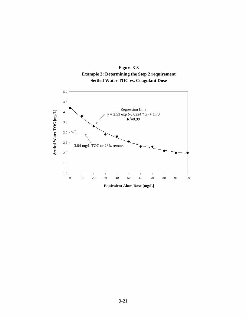
3-21

Figure 3-3Example 2: Determining the Step 2 requirement



0 10 20 30 40 50 60 70 80 90 100

Set

tled

Wat

er T

OC

[mg/

L]

1.0

1.5

2.0

2.5

3.0

3.5

4.0

4.5

5.0

Regression Liney = 2.53 exp (-0.0224 * x) + 1.70

R2=0.99

3.04 mg/L TOC or 28% removal

3-22

As shown in Table 3-5, the slope of the point-to-point curve reaches -0.03 between ferric

sulfate doses of 28.5 and 38 mg/L and does not fall below -0.03 (i.e. more than 0.3 mg/L TOC is not

removed in a 10 mg/L alum addition) at any point on the curve to the right of 38 mg/L. Therefore

the PODR occurs at the second (i.e. higher) dose of 38 mg/L. The calculated TOC removal at this

point where the slope criteria is satisfied is shown in Table 3-5 as 33 percent. The alternative Step

2 TOC removal should therefore be set at 33 percent. This is shown graphically on Figure 3-2 (note

that Figure 3-2 is drawn using equivalent alum dose). Based upon the results of this jar test, the

utility will apply to the State for an alternative TOC removal of 33 percent.

If in this example the slope had fallen below -0.03 at a point further to the right on the curve,

that point further to the right would have set the alternative TOC removal percentage (see Example

3). If the slope had been exactly -0.03 between these two points, the PODR would be set at the

second (i.e. higher) dose of 38 mg/L, since the slope of that entire line segment meets the requisite

slope (see Example 4).

Part B - Continuous curve

In this alternative data analysis approach, the utility received permission from the State to

use regression techniques to draw a best-fit continuous curve through the data points (data shown

in Table 3-5). To obtain a continuous curve, this utility fitted the experimentally observed residual

TOC levels versus the ferric sulfate solution dose data with an exponential decay model of the form

given in Equation 3-2 below. Commercially available curve-fitting programs can be used for this

type of regression analysis.

y = a*e-b(x) + C0 (3-2)

where:

x = coagulant dose in mg/Ly = residual TOC in mg/La, b, and C0 are fitting parameters, found using regression techniques.

C0 is significant since it represents the asymptote of the equation and therefore provides an estimate

of the refractory TOC (i.e. the amount that could not be easily removed by coagulation). The

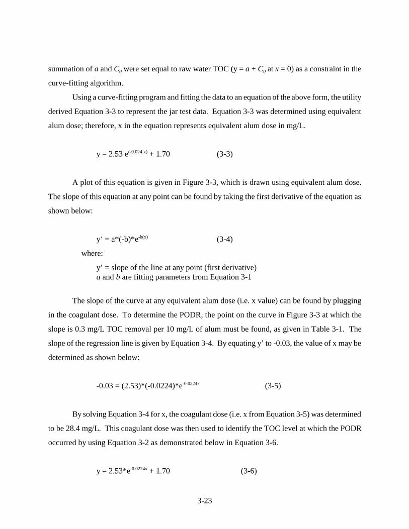
3-23

summation of a and C0 were set equal to raw water TOC (y = a + C0 at x = 0) as a constraint in the

curve-fitting algorithm.

Using a curve-fitting program and fitting the data to an equation of the above form, the utility

derived Equation 3-3 to represent the jar test data. Equation 3-3 was determined using equivalent

alum dose; therefore, x in the equation represents equivalent alum dose in mg/L.

y = 2.53 e(-0.024 x) + 1.70 (3-3)

A plot of this equation is given in Figure 3-3, which is drawn using equivalent alum dose.

The slope of this equation at any point can be found by taking the first derivative of the equation as

shown below:

y1 = a*(-b)*e-b(x) (3-4)

where:

y’ = slope of the line at any point (first derivative)a and b are fitting parameters from Equation 3-1

The slope of the curve at any equivalent alum dose (i.e. x value) can be found by plugging

in the coagulant dose. To determine the PODR, the point on the curve in Figure 3-3 at which the

slope is 0.3 mg/L TOC removal per 10 mg/L of alum must be found, as given in Table 3-1. The

slope of the regression line is given by Equation 3-4. By equating y’ to -0.03, the value of x may be

determined as shown below:

-0.03 = (2.53)*(-0.0224)*e-0.0224x (3-5)

By solving Equation 3-4 for x, the coagulant dose (i.e. x from Equation 3-5) was determined

to be 28.4 mg/L. This coagulant dose was then used to identify the TOC level at which the PODR

occurred by using Equation 3-2 as demonstrated below in Equation 3-6.

y = 2.53*e-0.0224x + 1.70 (3-6)

3-24

Solving for y (i.e. TOC level) at x = 28.4 in this equation gives y = 3.04 mg/L. Since the raw

water TOC is 4.2 mg/L, this corresponds to a TOC removal of 28 percent. The utility has now

determined that the Step 2 PODR TOC removal is 28 percent, and will apply to the State for an

alternative performance criteria of 28 percent TOC removal.

In some instances, jar test results may not indicate significant TOC removal until a certain

coagulant dose is reached. In other words, the TOC vs coagulant dose curve may be flat for the first

one or two applied doses. This phenomenon is sometimes referred to as the “threshold effect.”

Figure 3-4 shows an example of such a jar test result. If a utility is permitted by the State to use

regression analysis using this type of jar test result, they may need to use an alternative model such

as that described in Equation 3-7.

y = a*e-b(x-d) + C0 (3-7)

The first derivative of this equation is given by Equation 3-8:

y1 = a*(-b)*e-b(x-d) (3-8)

where:

x = coagulant dose in mg/Ly = residual TOC in mg/La, b, d, and C0 are fitting parameters, found using regression techniques.

As with Equation 3-2, the summation of a and C0 were set equal to the raw water TOC at all

doses prior to the ‘threshold’ dose (y = a + C0 when x �d) as the constraint in the curve-fitting

algorithm. Using a curve-fitting program and fitting the data to an equation of the form given in

Equation 3-7, the equation best representing the data points in Figure 3-4 is given in Equation 3-9

below.

y = 1.802 e(-0.0267*(x-10)) + 2.212 (3-9)

Equations 3-7, 3-8, and 3-9 can be used to determine an alternative compliance criterion

following the method described above for the example discussed in Figure 3-3. Cheng and co-

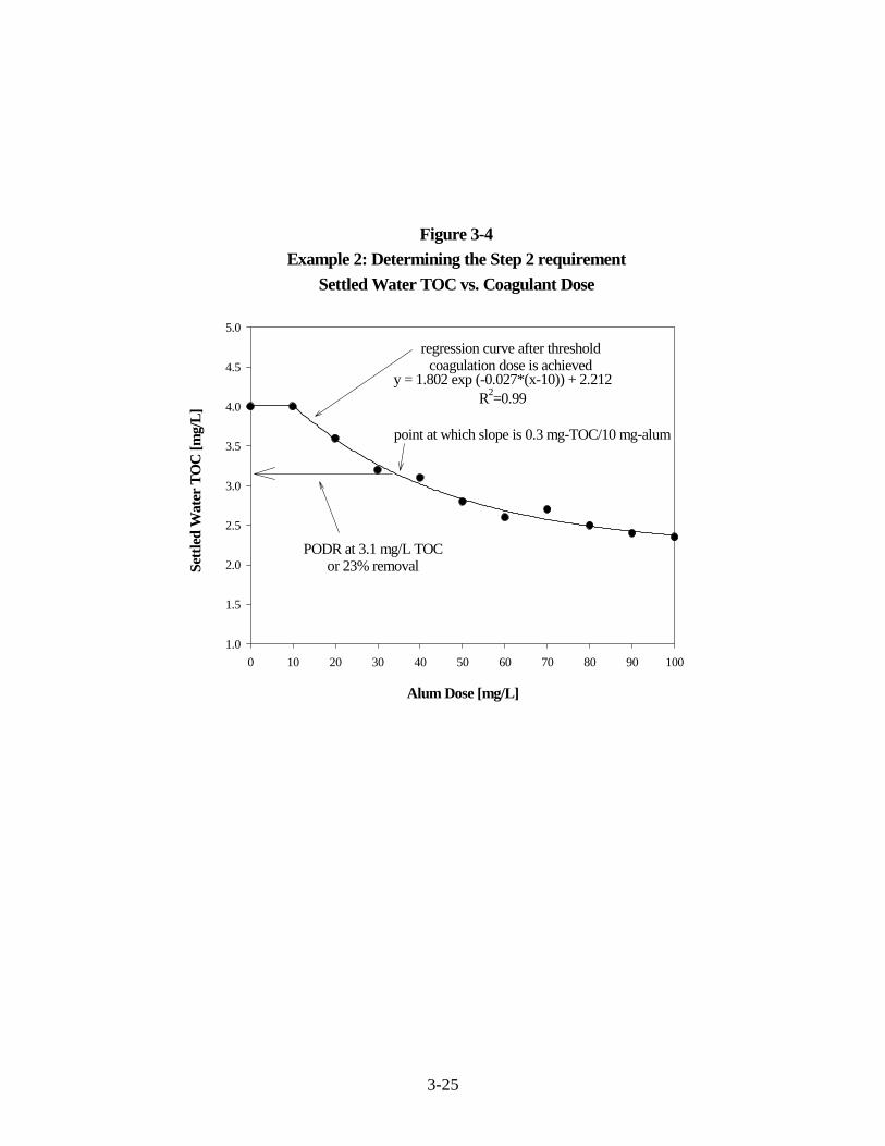
3-25

Figure 3-4Example 2: Determining the Step 2 requirement


Alum Dose [mg/L]

0 10 20 30 40 50 60 70 80 90 100

Set

tled

Wat

er T

OC

[mg/

L]

1.0

1.5

2.0

2.5

3.0

3.5

4.0

4.5

5.0

point at which slope is 0.3 mg-TOC/10 mg-alum

regression curve after thresholdcoagulation dose is achieved

y = 1.802 exp (-0.027*(x-10)) + 2.212R2=0.99


3-26

workers (1995) addressed other methods of curve fitting for jar test results. These methods include

polynomial expressions and isopleths in addition to the exponential decay models described above.

It should be noted that due to the peculiarity of a given data set, a single prescription for a curve-

fitting model may not be appropriate, and the user may need to search for the appropriate models

from those described here and in the literature.

3.2.3.3 Example 3 - Determining the Step 2 Requirement when the PODR is Met Twice

This utility determined that its running annual average compliance ratio was 0.85 at the end

of the first 12 months of monitoring and decided to conduct jar testing using the Step 2 procedure.

Jar tests were conducted following the protocol described in Section 3.2.2.2. A pH titration was

performed as described in Example 1 to the required “target pH” of 5.5 (see Table 2-2). Alum

addition of 90 mg/L was needed to reach a pH of 5.5, therefore, alum doses up to 90 mg/L (at 10

mg/L increments) were evaluated during jar testing. After performing the jar tests, TOC levels were

evaluated for each dose. The TOC results are given in Table 3-6 and shown graphically in Figure

3-5. Figure 3-5 presents the point-to-point TOC removal curve which will be used to determine the

PODR.

Table 3-6 shows the residual TOC level for each alum dose along with the slope between

each data point. The slope between each point is calculated according to Equation 3-1 as given in

Example 2. The slope of the point-to-point curve is calculated in this way to compare it to the Step

2 PODR criterion of 0.3 mg/L TOC removal per 10 mg/L alum (i.e., a slope of -0.03). As shown

in Table 3-6, the slope of the point-to-point curve reaches -0.03 between alum doses of 20 and 30

mg/L. However, the slope falls below or equals -0.03 further to the right on the curve at a higher

alum dose between 50 and 60 mg/L. This is shown graphically on Figure 3-5. The slope falls to -

0.03 again between alum doses of 50 and 60 mg/L. Since the slope does not equal or fall below -

0.03 beyond this point, this point is the PODR and will set the alternative TOC removal percentage.

Since the slope is exactly -0.03 between the two points at 50 and 60 mg/L, the alternative TOC

removal percentage is set at the second (i.e. higher) dose of 60 mg/L.

As shown in Table 3-6, at a dose of 60 mg/L the TOC removal is 27 percent. Therefore the

utility will apply to the State for an alternative performance criteria of 27 percent TOC removal.

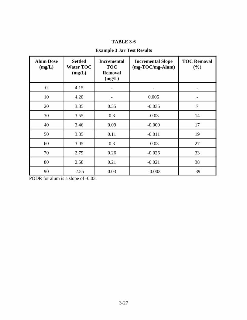
3-27

TABLE 3-6


Alum Dose(mg/L)

SettledWater TOC

(mg/L)

IncrementalTOC

Removal(mg/L)

Incremental Slope(mg-TOC/mg-Alum)

TOC Removal(%)

0 4.15 - - -

10 4.20 - 0.005 -

20 3.85 0.35 -0.035 7

30 3.55 0.3 -0.03 14

40 3.46 0.09 -0.009 17

50 3.35 0.11 -0.011 19

60 3.05 0.3 -0.03 27

70 2.79 0.26 -0.026 33

80 2.58 0.21 -0.021 38

90 2.55 0.03 -0.003 39

PODR for alum is a slope of -0.03.

3-28

Figure 3-5Example 3: Determining the Step 2 requirement when the PODR is met twice


Alum Dose [mg/L]

0 10 20 30 40 50 60 70 80 90

Set

tled

Wat

er T

OC

[mg/

L]

2.0

2.5

3.0

3.5

4.0

4.5

5.0



3-29

3.2.3.4 Example 4 -Adding Base to Maintain Minimum pH During Step 2 Jar Testing

This utility has a source water with low alkalinity. The alkalinity never rises above 60 mg/L

as CaCO3, and the utility is unable to achieve good TOC removal. After the first year of TOC

compliance sampling, the utility’s running annual average compliance ratio was 0.50. Therefore it

conducted the requisite Step 2 testing to set an alternative TOC removal percentage. A pH titration

was first performed to determine the ferric chloride dose range to be evaluated, as described in

Example 1. Based on titration results, it was apparent that the pH of the test sample would fall

below the target pH of 5.5 before additional TOC removal occurred. The treatment technique

requires that systems performing Step 2 testing on a sample with an alkalinity of less than 60 mg/L

as CaCO3 add a necessary amount of base to maintain the pH between 5.3 and 5.7. Incremental

coagulant addition should continue until the PODR is met, while the addition of base maintains the

pH between 5.3 and 5.7. The same type of base should be used during the Step 2 procedure as is

used at full-scale. The base doses required to maintain the “target pH” for the jar tests and resulting

pH levels are shown in Table 3-7. These doses were used during subsequent jar testing.

The utility conducted jar tests (while maintaining the sample pH in the required range

through base addition) to evaluate the Step 2 TOC removal requirement. After performing the jar

tests, TOC levels were evaluated for each dose. The TOC results are given in Table 3-8 and shown

graphically in Figure 3-6. Figure 3-6 presents the point-to-point TOC removal curve. Table 3-8

shows the residual TOC level for each ferric chloride dose. In addition, the equivalent alum dose

and incremental TOC removal is given at each point for calculation of the incremental slope in units

of mg-TOC/mg-alum. Calculation of the slope in terms of mg-alum allows direct comparison of

the incremental slope with the PODR requirement of 0.3 mg-TOC/10 mg-alum. The slope between

each point is calculated according to Equation 3-1 as given in Example 2.

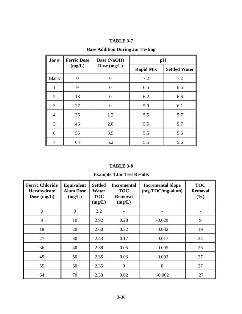
3-30

TABLE 3-7

Base Addition During Jar Testing

Jar # Ferric Dose(mg/L)

Base (NaOH)Dose (mg/L)

pH

Rapid Mix Settled Water

Blank 0 0 7.2 7.2

1 9 0 6.5 6.6

2 18 0 6.2 6.6

3 27 0 5.9 6.1

4 36 1.2 5.5 5.7

5 46 2.8 5.5 5.7

6 55 3.5 5.5 5.6

7 64 5.2 5.5 5.6

TABLE 3-8


Ferric ChlorideHexahydrateDose (mg/L)

EquivalentAlum Dose

(mg/L)

SettledWaterTOC

(mg/L)

IncrementalTOC

Removal(mg/L)

Incremental Slope(mg-TOC/mg-alum)

TOCRemoval

(%)

0 0 3.2 - - -

9 10 2.92 0.28 -0.028 9

18 20 2.60 0.32 -0.032 19

27 30 2.43 0.17 -0.017 24

36 40 2.38 0.05 -0.005 26

45 50 2.35 0.03 -0.003 27

55 60 2.35 0 0 27

64 70 2.33 0.02 -0.002 27

3-31

Figure 3-6Example 4: Adding base to maintain minimum pH during jar testing



0 10 20 30 40 50 60

Set

tled

Wat

er T

OC

[mg/

L]

1.0

1.5

2.0

2.5

3.0

3.5

4.0



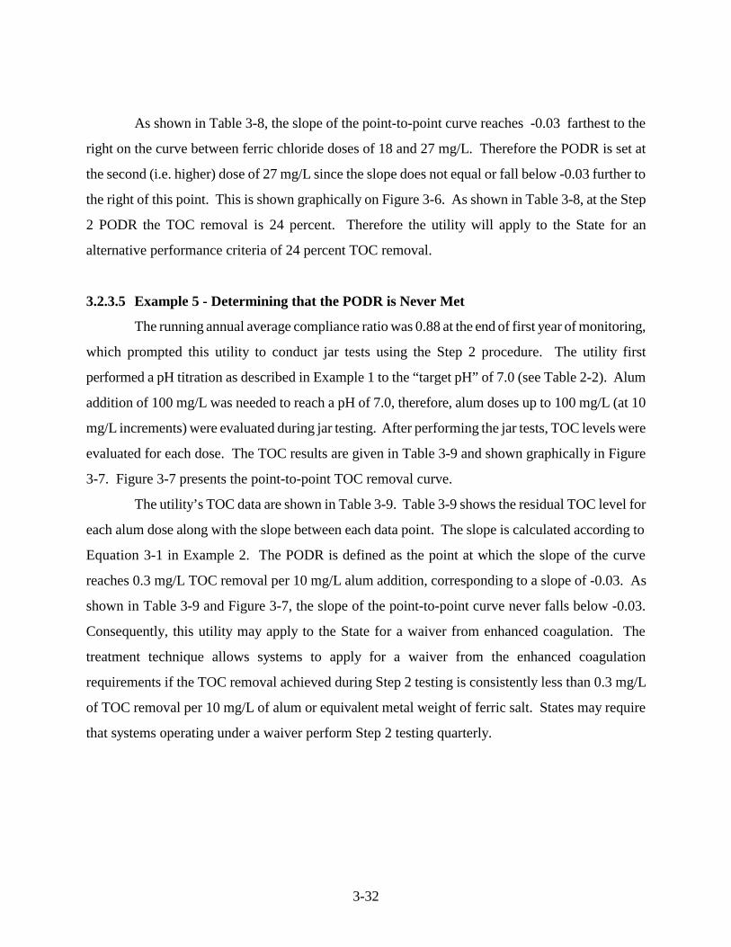
3-32

As shown in Table 3-8, the slope of the point-to-point curve reaches -0.03 farthest to the

right on the curve between ferric chloride doses of 18 and 27 mg/L. Therefore the PODR is set at

the second (i.e. higher) dose of 27 mg/L since the slope does not equal or fall below -0.03 further to

the right of this point. This is shown graphically on Figure 3-6. As shown in Table 3-8, at the Step

2 PODR the TOC removal is 24 percent. Therefore the utility will apply to the State for an

alternative performance criteria of 24 percent TOC removal.

3.2.3.5 Example 5 - Determining that the PODR is Never Met

The running annual average compliance ratio was 0.88 at the end of first year of monitoring,

which prompted this utility to conduct jar tests using the Step 2 procedure. The utility first

performed a pH titration as described in Example 1 to the “target pH” of 7.0 (see Table 2-2). Alum

addition of 100 mg/L was needed to reach a pH of 7.0, therefore, alum doses up to 100 mg/L (at 10

mg/L increments) were evaluated during jar testing. After performing the jar tests, TOC levels were

evaluated for each dose. The TOC results are given in Table 3-9 and shown graphically in Figure

3-7. Figure 3-7 presents the point-to-point TOC removal curve.

The utility’s TOC data are shown in Table 3-9. Table 3-9 shows the residual TOC level for

each alum dose along with the slope between each data point. The slope is calculated according to

Equation 3-1 in Example 2. The PODR is defined as the point at which the slope of the curve

reaches 0.3 mg/L TOC removal per 10 mg/L alum addition, corresponding to a slope of -0.03. As

shown in Table 3-9 and Figure 3-7, the slope of the point-to-point curve never falls below -0.03.

Consequently, this utility may apply to the State for a waiver from enhanced coagulation. The

treatment technique allows systems to apply for a waiver from the enhanced coagulation

requirements if the TOC removal achieved during Step 2 testing is consistently less than 0.3 mg/L

of TOC removal per 10 mg/L of alum or equivalent metal weight of ferric salt. States may require

that systems operating under a waiver perform Step 2 testing quarterly.

3-33

TABLE 3-9


Alum Dose(mg/L)

SettledWater TOC

(mg/L)

IncrementalTOC Removal

(mg/L)

Incremental Slope(mg-TOC/mg-alum)

TOC Removal(%)

0 4.05 - - -

10 4 0.05 -0.005 1

20 3.85 0.15 -0.015 5

30 3.7 0.15 -0.015 9

40 3.8 - 0.01 6

50 3.6 0.2 -0.02 11

60 3.4 0.2 -0.02 16

70 3.3 0.1 -0.01 19

80 3.2 0.1 -0.01 21

90 3.2 0 0 21

100 3.2 0 0 21

3-34

Figure 3-7Example 5: Determining that the PODR is never met


Alum Dose [mg/L]

0 10 20 30 40 50 60 70 80 90 100

Set

tled

Wat

er T

OC

[mg/

L]

1.0

1.5

2.0

2.5

3.0

3.5

4.0

4.5

5.0

curve never reaches 0.3 mg-TOC/10 mg-alum


3-35

3.3 ENHANCED PRECIPITATIVE SOFTENING

Enhanced precipitative softening requires that softening systems achieve TOC removals

ranging from 15 to 30 percent based upon their raw water TOC level (see Table 2-1). Systems that

cannot achieve these removal levels may demonstrate compliance by meeting the alternative

compliance criteria listed in Section 2.4.

Utilities using enhanced softening are not allowed to perform the bench- or pilot-scale

testing outlined in Section 3.2 for regulatory compliance. It is strongly recommended, however, that

these utilities perform bench- or pilot-scale studies to characterize the performance of the plant under

enhanced precipitative softening conditions, and to ascertain its ability to achieve the TOC removals

or meet one of the alternative compliance criteria. The treatment technique does not require systems

to modify their existing treatment processes to include a chemical or a process (e.g., soda ash) that

is not currently in use. For example, if a treatment plant is a lime-softening facility that does not use

soda ash, processes would not have to be modified to include lime-soda ash softening just to meet

the TOC removal requirements.

3.3.1 Full-Scale Evaluation of TOC Removal Requirements

Initially, utilities should evaluate TOC removal between the raw water source and the final

TOC monitoring location in the full-scale treatment plant. After collecting raw and treated water

samples and analyzing for TOC, the percent removal of TOC may be calculated. If the Step 1

removal requirements (Table 2-1) are met, then the utility is in compliance. If the utility is very close

to meeting the percent removal of TOC requirements, full-scale increases of lime and/or coagulant

may be made to increase the amount of TOC removal. If the full-scale coagulant and lime

adjustments achieve the required TOC removal, then the utility is in compliance and no further

evaluation will be necessary. However, if the lime-coagulant doses do not achieve the TOC removal

required and more than “minor” adjustments are necessary to achieve the required removal of TOC,

then bench- or pilot-scale evaluation is advisable.

3-36

3.3.2 Bench-Scale and Pilot-Scale Testing

If a precipitative softening system is unable to meet the TOC requirements specified in

Table 2-1 under current operation or with increased lime and coagulant doses, and does not meet any

of the alternative compliance criteria, treatability testing should be performed. Treatability testing

can be performed on a batch basis or on a continuous flow, pilot-scale basis. Treatability testing will

assist the utility in determining lime, soda ash, and/or coagulant dosages that will achieve the TOC

removals specified in Table 2-1.

Bench-scale procedures described below are based on the ASTM D 2035-80 method,

"Standard Practice for Coagulation-Flocculation Jar Test of Water." These procedures have been

modified for evaluations of treatment plants using lime softening.

3.3.2.1 Apparatus and Reagents

The following equipment and chemicals are required, at a minimum, to perform the testing:

& Jar test apparatus with 1 liter (L) beakers or 2 L square mixing jars.

& pH meter. The pH meter should be calibrated daily with fresh buffers. A two-pointcalibration using buffer solutions with pH = 4.0 and pH = 7.0 is necessary at a minimum; athree-point calibration using pH = 4.0, pH = 7.0, and pH = 10.0 is preferred.

& Lime stock solution made so that, for example, 1.0 mL into 2 L = 20 mg/L of lime (i.e., stockconcentration is 40 mg/mL). The type (hydrated or slaked) and the grade (90 to 100 percentactive) of lime will affect the preparation of the stock solution.

& Ferric chloride or ferric sulfate stock solution made so that, for example, 1.0 mL into 2 L =10 mg/L of ferric coagulant (i.e., stock concentration is 20 mg/mL).

& Sample bottles suitable for analysis of coagulated water for alkalinity, hardness (calcium andmagnesium), and pH measurement.

& Sample bottles suitable for TOC, DOC, and UV-254 analysis.

& 25 and 50 mL pipettes, with 10 mL graduated pipette bulbs.

& 1L graduated cylinders.

& Miscellaneous beakers and other glassware.

& 20 L carboys with siphons for dispensing water. A suitable laboratory tap also may be used.

3-37

& Magnetic stirrer with stirring bars.

3.3.2.2 Protocol for Bench-Scale (Jar) Testing

The following method can be used to evaluate incremental TOC removal by lime softening

using the bench-scale apparatus described above. Most available data on TOC removal in lime-

softening plants indicate that varying the lime dose has a greater effect on TOC removal than does

varying the coagulant dose.

Step 1. Gather testing supplies.

Step 2. Prepare lime stock solution.

Example - Developing a Lime Stock Solution.

Given: A recent quality assurance analysis from the lab indicates that the unslakedlime delivered to a water plant is 90% active chemical. The density of thelime is approximately 60 lb/ft3.

Assume:A stock concentration is desired such that 1.0 mL into 2 L equals 20 mg/Lof lime.

Calculate the amount of lime needed to make 1 L of a stock solution.

CstockVstock = CjarVjar C = Concentration; V = Volume)Cstock = CjarVjar ÷ Vstock Cstock = (20 mg/L lime x 2 L) ÷ 1 mL lime stock solutionCstock = 40 mg/mL lime

Therefore, add 40 g of active lime to 1 L of water.

Massunslaked lime = 40 g active lime ÷ 0.90 = 44 g

Therefore, add 44 g of the unslaked lime into a 1 L volumetric flask, then fill theflask to the 1 L mark. Mix well. The resulting solution is a 40 g/L stock solution ofactive lime; adding 1 mL of stock into a 2 L jar will result in a 20 mg/L dose of lime.

Step 3. Collect 20 to 30 liters of raw water for the jar testing. The temperature of the sample shouldbe maintained at ambient conditions prior to and during testing. If the collected water mustbe stored for subsequent testing, the sample should be refrigerated (approximately 4oC).The temperature of the sample should be adjusted to the ambient temperature during

3-38

collection before starting any testing with the sample. Every effort should be made toconduct tests with freshly collected water.

Step 4. Measure pH and alkalinity of the raw water sample.

Step 5. Determine the lime dosages to evaluate for enhanced softening by titrating lime into 1000or 2000 mL of raw water (depending on the available jar test apparatus) on a magnetic stirplate in 10 mg/L increments. If coagulant is added concurrently with lime or preceding limeaddition in the full-scale plant, the plant dose of coagulant should be added to the beakersprior to lime titration. On the other hand, if coagulant is added in a subsequent stagefollowing lime (or lime-soda ash) softening, no coagulant addition is needed for this limetitration.

Measure and record the pH after each incremental lime dose. The highest pH to beinvestigated should not exceed approximately 11.2, which is the optimum pH formagnesium hydroxide removal.

Step 6. Pour the raw water sample into a series of six beakers or mixing jars and place the jars onthe jar test apparatus. Add the lime dosages needed to achieve pH increments of 0.2(including coagulant addition) in individual beakers. For example, the softening pH in eachof the six jars could be 10.2, 10.4, 10.6, 10.8, 11.0, and 11.2.

Rapid mix, flocculate, and settle using times corresponding to the detention time at the plantmaximum daily flow rate. Rapid mix and flocculation mixing intensities and durationsshould be matched to those in the plant, if known. If coagulant is added concurrently withlime or preceding lime addition in the full-scale plant, the plant dose of coagulant shouldbe added to each beaker or mixing jar prior to lime addition. On the other hand, if coagulantis added in a subsequent stage following lime (or lime-soda ash) softening, coagulantaddition should be done after flocculation is complete with lime addition. A subsequentflocculation stage (corresponding to full-scale) will be necessary to complete thecoagulation process. Alternatively, coagulant can be added during bench-scalerecarbonation (step 7). The timer on the process should be started after the chemicals areadded.

If the plant intensities and durations are not known, the following jar-test mixing conditionscan be used for the softening and/or coagulation steps:

& Rapid mix at 120 rpm for 30 seconds& Flocculate at 80 rpm for 2 minutes

3-39

& Flocculate at 60 rpm for 20 minutes& Flocculate at 40 rpm for 20 minutes

All jars, regardless of mixing conditions, should settle for 60 minutes, without stirring,prior to sampling.

Step 7. After settling, carefully remove as large a batch of supernatant as possible and adjust pH byrecarbonation. Be careful not to disturb the settled floc, and to avoid suspended floc, whilesampling. Each sample should be titrated on a magnetic stir plate while bubbling CO2

through a diffuser, stirring and measuring pH until the pH of the plant recarbonated wateris achieved. Alternatively, if CO2 addition could not be performed at bench-scale, pHadjustment should be done by adding dilute hydrochloric or sulfuric acid until the pH of thewater matches full-scale recarbonated pH values.

Step 8. Sample the supernatant for TOC, total hardness, and magnesium hardness analysis using25 or 50 mL pipettes, a siphon apparatus, or sampling ports located on the side of themixing jars. Preserve and refrigerate the samples for subsequent TOC analysis as describedin Chapter 5.

Step 9. Withdraw additional supernatant samples for pH, hardness (calcium and magnesium),alkalinity, and UV-254 and DOC (for SUVA calculations), and analyze within appropriateholding times.

TOC removals achieved in the jar tests may provide a reasonable representation of TOC

removals achievable on a plant-scale. Filtration may provide some additional removal of TOC

beyond that achieved in the jar tests, and a system may wish to include TOC removal by filtration

as part of their full-scale compliance with the enhanced softening requirements.

3.3.2.3 Protocol for Pilot-Scale Testing

It is important to simulate physical conditions such as mixing, detention times, and solids

recycle in the pilot plant corresponding to those conditions in the full-scale water treatment plant.

Alternative softening and coagulation conditions can be evaluated using the pilot plant by varying

lime (or lime, soda ash combination) and/or coagulant dosages. Increments of lime (or lime, soda

ash combination) dosages should be selected to result in increments of softening pH that are at least

0.2 units apart. For example, softening pHs of 10.2, 10.4, 10.6, 10.8, 11.0 and 11.2 could be

evaluated. The coagulant dose range should be selected based upon the range of operation of the

full-scale water treatment plant. Appropriate coagulant aid polymers may also be added during pilot

3-40

tests. The pilot plant should be operated long enough for each of the alternative conditions to

achieve steady-state. This may require a minimum of three to four times the theoretical detention

time of the pilot plant. After achieving steady-state, samples should be collected as discussed in

Section 3.3.2.2.

Chapter 4

MONITORING AND REPORTING


4.0 MONITORING AND REPORTING4.1 Introduction .................................................................................................4-14.2 Monitoring Plans .........................................................................................4-14.3 Sampling Locations and Monitoring Frequency .........................................4-2

4.3.1 TOC.................................................................................................4-24.3.2 Alkalinity.........................................................................................4-24.3.3 Reduced Monitoring for TOC and Alkalinity .................................4-24.3.4 Monitoring for Alternative Compliance Criteria.............................4-2

4.3.4.1 Additional Alternative Compliance Criteria forSoftening Plants................................................................4-3

4.3.4.2 Monitoring for TTHM and HAA5 ...................................4-44.4 Enhanced Coagulation and Softening..........................................................4-5

4.4.1 Reporting Requirements for TOC Compliance...............................4-54.4.2 Reporting for Alternative Compliance Criteria...............................4-64.4.3 Compliance Calculations for Enhanced Coagulation and

Softening .........................................................................................4-84.4.4 Running Annual Average Calculation Flowcharts..........................4-8

4.5 Example Calculations................................................................................4-13

List of Tables

4-1 Monitoring Locations and Sampling Frequency for TTHM and HAA5..............4-44-2 Reporting Requirements.......................................................................................4-74-3 DBP Precursor Removal Compliance Calculations for Example

Water Utility: Enhanced Coagulation, Year 1..................................................4-144-4 DBP Precursor Removal Compliance Calculations for Example

Water Utility: Enhanced Coagulation, Year 2..................................................4-154-5 DBP Precursor Removal Compliance Calculations for Example

Water Utility: Enhanced Precipitative Softening, Year 1 ................................4-174-6 DBP Precursor Removal Compliance Calculations for Example

Water Utility: Enhanced Precipitative Softening, Year 2 ................................4-18

List of Figures

4-1 Running Annual average Compliance Calculation -First Year of TOC Compliance Monitoring.......................................................4-10

4-2 Running Annual Average Compliance CalculationAfter First Year of TOC Compliance Monitoring, EC and ES..........................4-11

4-3 Calculation of Running Annual Average Under Step 2 -EC Plants Only...................................................................................................4-12

4-1

4.0 MONITORING AND REPORTING

4.1 INTRODUCTION

Compliance with the enhanced coagulation/enhanced softening treatment technique is based

on a running annual average of quarterly averages; one full year of monitoring data is

necessary to demonstrate compliance. Water treatment plants must sample source and

finished water for TOC and source water alkalinity. Alkalinity samples must be collected

at the same time and location as the source water TOC samples. If a plant intends to

establish compliance with an alternative compliance criterion, it also may need to sample for

TTHMs, HAA5, magnesium hardness removal, DOC, and UV-254.

4.2 MONITORING PLANS

Plants required to monitor for TOC removal compliance must develop and

implement a monitoring plan. The plant must maintain the plan and make it available for

inspection by the State and the general public. Subpart H systems serving more than 3,300

people must submit a copy of the monitoring plan to the State no later than the first time data

are submitted to demonstrate compliance with any portion of the DBPR. Following its

review, the State may require changes to the monitoring plan. The State also may require

monitoring plans to be submitted by other systems. The monitoring plan must include at

least the following elements:

� Locations for collecting samples used to demonstrate compliance (frequency andday(s) of sampling also should be included for source and finished water TOCsampling).

� An explanation of the enhanced coagulation/enhanced softening treatment techniqueto be used, and how the system will calculate compliance with MCLs and MRDLs.

The monitoring plan sampling locations for TTHM and HAA5 must be

representative of the entire distribution system if water is provided to consecutive systems,

or if the system is approved for monitoring as a consecutive system.

4-2

4.3 SAMPLING LOCATIONS AND MONITORING FREQUENCY

4.3.1 TOC

Plants required to implement enhanced coagulation or enhanced softening must

monitor for TOC in the source water prior to any treatment, including oxidant addition.

Treated water TOC also must be monitored no later than the combined filter effluent

turbidity monitoring location. These samples (source water and treated water) are referred

to as paired samples. Plants must take a minimum of one paired sample per month per plant

at a time representative of normal operating conditions and influent water quality.

4.3.2 Alkalinity

At the time of paired sampling for TOC, the plant also must sample for source water

alkalinity at the same location.

4.3.3 Reduced Monitoring for TOC and Alkalinity

Plants may reduce TOC monitoring under the following conditions:

1. Plants with a treated water TOC running annual average of less than 2.0 mg/Lfor two consecutive years may reduce monitoring for both TOC and alkalinityto one paired sample per plant per quarter, or

2. Plants with a treated water TOC running annual average of less than 1.0 mg/Lfor one year may reduce monitoring for both TOC and alkalinity to one pairedsample per plant per quarter.

Plants under reduced monitoring must revert to routine monitoring in the month

following the quarter when the average treated water TOC is greater than or equal to 2.0

mg/L.

4.3.4 Monitoring for Alternative Compliance Criteria

Running annual averages are used to demonstrate compliance with alternative

compliance criteria. Four quarters of data are needed to demonstrate that the alternative

compliance criteria are being met on a running annual average basis. However, alternative

4-3

compliance criteria also may be used to demonstrate compliance for a single month. For

example, a plant might not achieve the required Step 1 TOC removal in a given month, but

may determine that the finished water SUVA for that monthly sample is less than or equal

to 2.0 L/mg-m. The plant is therefore able to assign a value of 1.0 (a value of 1.0 or greater

indicates compliance with the TOC removal requirements) for the monthly removal ratio to

use in the running annual average compliance calculation. For months in which alternative

compliance criteria are used, a monthly removal ratio of 1.0 must be used for compliance

calculations (see Section 4.4.3, step 3). A plant can demonstrate compliance with enhanced

coagulation and enhanced precipitative softening if any one of the alternative compliance

criteria listed in Section 2.4 is met. These criteria are listed below. See Section 2.4 for a

complete description of the requirements.

1. Source water TOC < 2.0 mg/L.

2. Treated water TOC < 2.0 mg/L.

3. Source water SUVA � 2.0 L/mg-m.

4. Treated water SUVA � 2.0 L/mg-m.

5. Source water TOC < 4.0 mg/L, source water alkalinity > 60 mg/L (as CaCO3),TTHM < 40 ug/L, HAA5 < 30 ug/L.

6. TTHM � 40 ug/L and HAA5 � 30ug/L with only chlorine for primary disinfectionand maintenance of a residual.

4.3.4.1 Additional Alternative Compliance Criteria for Softening Plants

Utilities that use softening may demonstrate compliance if they meet any of the six

alternative compliance criteria listed above or one of the two alternative compliance criteria

listed below (see also Section 2.4):

1. Softening that results in lowering the treated water alkalinity to less than 60 mg/L (as CaCO3),measured monthly and calculated quarterly as a running annual average.

2. Softening that results in removing at least 10 mg/L of magnesium hardness (as CaCO3),measured monthly and calculated quarterly as a running annual average.

4-4

4.3.4.2 Monitoring for TTHM and HAA5

Utilities monitoring to meet alternative compliance requirements 5 or 6 in Section 4.3.4

must use the TTHM and HAA5 samples used to calculate compliance with the MCLs to determine

compliance with alternative compliance criteria 5 and 6. Monitoring locations and sampling

frequency for TTHM and HAA5 depend on the source water type and the population served, as shown

in Table 4-1.

TABLE 4-1

Monitoring Locations and Sampling Frequency for TTHM and HAA5

Type of SystemMinimum Monitoring

FrequencySample Location in the

Distribution System

Subpart H system servingat least 10,000 persons

Four water samples perquarter per treatment plant

At least 25 percent of all samples collected each quarter atlocations representing maximum residence time. Remainingsamples taken at locations representative of at least averageresidence time in the distribution system and representingthe entire distribution system, taking into account numberof persons served, different sources of water, and differenttreatment methods.1

Subpart H system servingfrom 500 to 9,999 persons

One sample per quarterper treatment plant1

Locations representing maximum residence time.1

Subpart H system servingfewer than 500 persons

One sample per year pertreatment plant duringmonth of warmest watertemperature

Locations representing maximum residence time.1 If thesample (or average of annual samples, if more than onesample is taken) exceeds MCL, system must increasemonitoring to one sample per treatment plant per quarter,taken at a point reflecting the maximum residence time inthe distribution system, until system meets reducedmonitoring criteria specified in the regulation.

System using only groundwater not under directinfluence of surface water,using chemical disinfectantand serving at least 10,000people

One sample per quarterper treatment plant2

Locations representing maximum residence time.1

System using only groundwater not under directinfluence of surface water,using chemical disinfectantand serving fewer than10,000 people

One sample per year pertreatment plant2 duringmonth of warmest watertemperature

Locations representing maximum residence time.1 If thesample (or average of annual samples, if more than onesample is taken)exceeds MCL, system must increasemonitoring to one sample per treatment plant per quarter,taken at a point reflecting the maximum residence time inthe distribution system, until system meets reducedmonitoring criteria specified in the regulation.

1 If a system elects to sample more frequently than the minimum required, at least 25 percent of all samples collected each quarter(including those taken in excess of the required frequency) must be taken at locations that represent the maximum residence time of the waterin the distribution system. The remaining samples must be taken at locations representative of at least average residence time in thedistribution system. 2 Multiple wells drawing water from a single aquifer may be considered one treatment plant for determining the minimum number of

samples required, with State approval in accordance with criteria developed under Part 142.16(h)(5), title 40 Code of Regulations.

4-5

4.4 ENHANCED COAGULATION AND SOFTENING

4.4.1 Reporting Requirements for TOC Compliance

Reports from plants monitoring monthly or quarterly to demonstrate compliance

with Step 1 or Step 2 TOC removal requirements must provide the following information to

the State. Monitoring results must be reported to the State within ten days after the end of

the quarter in which samples were collected. Plants sampling less frequently than quarterly

must report monitoring results to the State within ten days of the end of the monitoring

period in which the samples were collected. Reporting information includes:

1. The number of paired (source water and treated water) samples taken during the lastquarter.

2. The location, date, and result of each paired sample taken during the last quarter andthe associated source water alkalinity.

3. For each month in the reporting period that paired samples were taken, the arithmeticaverage of the actual TOC percent removal for each paired sample and the requiredTOC percent removal.

4. Calculations for determining compliance with the TOC percent removal requirements(see discussion below).

5. Whether the system is in compliance with the enhanced coagulation/enhancedsoftening TOC removal requirements for the last four quarters for which TOCpercent removal calculations were required.

6. TOC percent removal calculations are not required for quarters in which all threemonths use an alternative compliance criterion to demonstrate compliance. Systemsthat use an alternative criterion to demonstrate compliance for a particular monthshould specify which criterion was used (see step 3 in Section 4.4.3).

The system must ensure that all results are compiled and presented to the State. The

State, however, may choose to perform items 3, 4, and 5 above in lieu of having the system

report that information.

4-6

4.4.2 Reporting for Alternative Compliance Criteria

Plants wishing to demonstrate compliance with one of the alternative compliance

criteria, on a running annual average basis, must report the following information to the

State. Monitoring results must be reported to the State within ten days after the end of the

quarter in which samples were collected. Plants sampling less frequently than quarterly must

report monitoring results to the State within ten days of the end of the monitoring period in

which the samples were collected. Reporting information includes:

1. The alternative compliance criterion that the system is using to demonstratecompliance.

2. The number of paired samples taken during the last quarter.

3. The location, date, and result of each paired sample and associated alkalinity takenduring the last quarter.

4. The running annual arithmetic average based on monthly averages (or quarterlysamples) of source water TOC for systems using alternative compliance criteria 1 or5, or of treated water TOC for systems using alternative compliance criterion 2 (seeSection 4.3.4).

5. The running annual arithmetic average based on monthly averages (or quarterlysamples) of source water SUVA for systems using alternative compliance criterion3, or of treated water SUVA for systems using alternative compliance criterion 4 (seeSection 4.3.4).

6. The running annual average of source water alkalinity for systems using alternativecompliance criterion 5 (see Section 4.3.4), and of treated water alkalinity for systemsusing alternative compliance criterion 1 for softening systems (see Section 4.3.4.1).

7. The running annual average for both TTHMs and HAA5 for systems using alternativecompliance criteria 5 or 6 (see Section 4.3.4).

8. The running annual average of the amount of magnesium hardness removal (asCaCO3, in mg/L) for systems using alternative compliance criterion 2 for softeningsystems (see Section 4.3.4.1).

9. Whether the system is in compliance with the particular alternative compliancecriterion in Section 4.3.4 or 4.3.4.1.

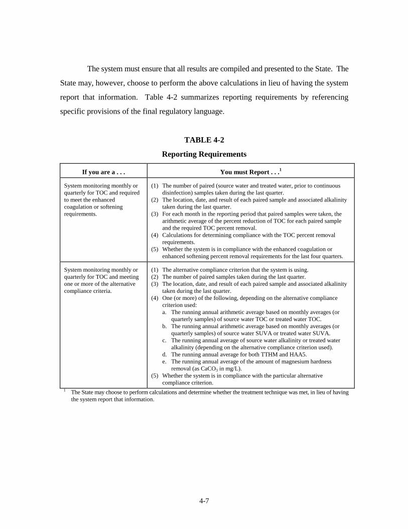
4-7

The system must ensure that all results are compiled and presented to the State. The

State may, however, choose to perform the above calculations in lieu of having the system

report that information. Table 4-2 summarizes reporting requirements by referencing

specific provisions of the final regulatory language.

TABLE 4-2

Reporting Requirements

If you are a . . . You must Report . . .1

System monitoring monthly orquarterly for TOC and requiredto meet the enhancedcoagulation or softeningrequirements.

(1) The number of paired (source water and treated water, prior to continuousdisinfection) samples taken during the last quarter.

(2) The location, date, and result of each paired sample and associated alkalinitytaken during the last quarter.

(3) For each month in the reporting period that paired samples were taken, thearithmetic average of the percent reduction of TOC for each paired sampleand the required TOC percent removal.

(4) Calculations for determining compliance with the TOC percent removalrequirements.

(5) Whether the system is in compliance with the enhanced coagulation orenhanced softening percent removal requirements for the last four quarters.

System monitoring monthly orquarterly for TOC and meetingone or more of the alternativecompliance criteria.

(1) The alternative compliance criterion that the system is using.(2) The number of paired samples taken during the last quarter.(3) The location, date, and result of each paired sample and associated alkalinity

taken during the last quarter.(4) One (or more) of the following, depending on the alternative compliance

criterion used:a. The running annual arithmetic average based on monthly averages (or

quarterly samples) of source water TOC or treated water TOC.b. The running annual arithmetic average based on monthly averages (or

quarterly samples) of source water SUVA or treated water SUVA.c. The running annual average of source water alkalinity or treated water

alkalinity (depending on the alternative compliance criterion used).d. The running annual average for both TTHM and HAA5.e. The running annual average of the amount of magnesium hardness

removal (as CaCO3 in mg/L).(5) Whether the system is in compliance with the particular alternative

compliance criterion.

1 The State may choose to perform calculations and determine whether the treatment technique was met, in lieu of havingthe system report that information.

4-8

4.4.3 Compliance Calculations for Enhanced Coagulation and Softening

Compliance with the DBP precursor removal requirements is based on achieving the

required TOC removal. Compliance is calculated quarterly by the following method:

1. Determine actual monthly TOC percent removal for each compliance sample, usingthe equation:

percent removal = (1 - (treated water TOC/source water TOC)) x 100.

2. Determine the required monthly TOC percent removal based on either Step 1 or Step2 requirements (see Section 2.3).

3. To determine the monthly removal ratio, divide the answer from step 1 by the answerfrom step 2 for each compliance sample taken. For those months that an alternativecompliance criterion is used, a value of 1.0 shall be assigned. If more than onecompliance sample is taken during the month, calculate the arithmetic average ofremoval ratios and use that average for the monthly value.

4. Sum the answers from step 3 for the last three months, and divide by three. Theresult is the quarterly removal ratio.

5. Sum the results of step 4 for the last four quarters, and divide by four.

6. If the result from step 5 is greater than or equal to 1.0, the system is in compliancewith the TOC percent removal requirements.

4.4.4 Running Annual Average Calculation Flowcharts

Utilities can use the flowcharts shown in Figures 4-1, 4-2, and 4-3 to calculate their

running annual average for TOC removal compliance. Example compliance calculations are

provided in Section 4.5.

The flowchart in Figure 4-1 shows how utilities can calculate their annual running

average for the first year of compliance monitoring. Note that alternative compliance criteria

can be used on a monthly basis during the first year (and subsequent years) of compliance

monitoring. A monthly removal ratio of 1.0 must be used for those months in which

alternative compliance criteria are used. Compliance with the TOC removal requirements

is based on a running annual average, therefore utilities need 12 months of TOC monitoring

4-9

data to make a compliance determination. Since Step 2 bench- or pilot-scale testing is only

required when an enhanced coagulation system fails to achieve a running annual average

greater than or equal to 1.0 (i.e., the system is out of compliance), Step 2 testing generally

will not be performed until the second year of TOC compliance sampling. If the State

approves the Step 2 TOC removal percentage, the State may make that percentage retroactive

for determining compliance.

The flowchart in Figure 4-2 illustrates how utilities can compute their running annual

average after the first year of TOC compliance sampling. Enhanced coagulation plants are

required to perform Step 2 testing if their running annual average falls below 1.0. Figure 4-3

shows the calculation of a running annual average when compliance is determined by the

Step 2 TOC removal percentage. Plants operating under a Step 2 alternative TOC removal

percentage should consult with the State when their running annual average achieves a value

equal to or greater than 1.0 to determine whether they should return to the Step 1

requirements for compliance calculations. Quarterly Step 2 testing is recommended the

firstyear a plant determines compliance with the Step 2 TOC procedure. EPA recommends

that this frequency not be reduced to less than annually.

4-10

Perform m onthly raw andtreated w ater TOC sam pling

Is theStep 1

rem oval percentageachieved?

Record actual TOC rem ovaldiv ided by required TOC

rem oval for m onthly rem oval ratio

Y es

A reany of thealternativecom pliance

criteriasatisfied?

N o

Record 1.0 as them onthly rem oval ratio

Y es

N o

Record actual TOC rem ovaldiv ided by required TOC

rem oval for m onthly rem oval ratio

H asutility

com pleted 12m onths of TOC

sam pling?

Com pute running annual average (RA A )

Y es

N o

Is

RA A � 1.0? G o to Figure 4-3(EC system s only)

G o to Figure 4-2 Y es N o

F igure 4-1. Running A nnual AverageCom pliance Calculation - First Yearof TOC Com pliance M onitoring

4-11

Perform monthly raw andtreated water TOC sampling

Is theStep 1

removal percentageachieved?

Record actual TOC removaldivided by required TOC

removal for monthly removal ratio

Yes

Areany of thealternativecompliance

criteriasatisfied?

No

Record 1.0 as themonthly removal ratio

Yes

No

Isquarterly

average and newRAA computed

this month?

Yes

No

Is

RAA � 1.0?

Figure 4-2. Running Annual AverageCompliance Calculation After First Yearof TOC Compliance Monitoring, EC and ES

Does theutility perform

enhancedsoftening?

Utility is outof compliance

Yes

YesGo to Figure 4-3(EC systems only)

No

No

4-12

Is Stateapproved Step 2

removal percentageachieved?



Yes

Areany of thealternativecompliance

criteriasatisf ied?

No

Record 1.0 as the monthly removal ratio

Yes

No

Submit results of Step 2 testingto State w ithin 3 months of

achieving RAA < 1.0

Perform monthlyTOC sampling



Is aquarterly

average and newRAA calculated

this month?

Isnew

RAA � 1.0?

System is outof compliance

No

Yes

Consult w ith State todeterm ine if system returnsto Step 1 TOC requirements

Yes

No

Figure 4-3. Calculation of Running Annual Average Under Step 2 - EC Plants Only

4-13

4.5 EXAMPLE CALCULATIONS

Example 1 - Enhanced Coagulation

Tables 4-3 and 4-4 show sample running annual average calculations for a plant

experiencing frequent changes in source water TOC and alkalinity. In year one (Table 4-3),

compliance is based upon achieving a running annual average of 1.0 or greater after TOC

sampling in month 12 is complete (at the end of the fourth quarter). The monthly removal

ratios shown in column C are calculated from the required Step 1 TOC removal matrix

(Table 2-1) and by meeting alternative performance criteria. Months in which an alternative

compliance criterion is used are assigned a monthly removal ratio of 1.0.

The running annual average calculation in the second year (Table 4-3) uses monthly

removal ratios calculated from the Step 1 removal percentages and alternative compliance

criteria 2 and 4 (discussed in Section 2.4). The quarterly average in the third quarter of year

one (Table 4-3) is less than 1.0, however, the running annual average is greater than 1.0 and

the system is in compliance at the end of the first year. The second running annual average

(calculated after the first quarter of the second year) is below 1.0, and the plant uses the Step

2 procedure to establish alternative TOC removal requirements, with State approval. Note

that the plant is in violation the first quarter of the second year if the State does not allow the

Step 2 TOC removal percentage to be applied retroactively.

Alternative compliance criteria 5 and 6 (discussed in Section 2.4) may not be used

on a monthly basis.

TABLE 4–3

DBP Precursor Removal Compliance Calculations for Example Water Utility:Enhanced Coagulation Year 1

Month

Source Water TreatedWater TOC

(mg/L)

(A)Actual

% TOCRemoval

(B)Required% TOCRemoval

Basis forRequired %

Removal

(C)Removal

Ratio(A) / (B)

(D) a

QuarterlyAverage

Ratio

(E) b

RAA Ratio(Last 4

Quarters)Alk

(mg/L)TOC

(mg/L)

January 50 3.9 2.1 46.2% 35.0% Step 1 1.32 – –

February 40 3.3 2.1 36.4% 35.0% Step 1 1.04 – –

March 58 4.2 2.0 52.4% 45.0% Step 1 1.16 1.17 –

April 65 4.1 2.2 46.3% 45.0% Step 1 1.03 – –

May 63 4.3 2.2 48.8% 45.0% Step 1 1.09 – –

June 67 4.0 2.3 42.5% NA Altern. 4c 1.0 1.04 –

July 46 3.5 2.2 37.1% 35.0% Step 1 1.06 – –

August 33 4.8 2.6 45.8% 45.0% Step 1 1.02 – –

September 70 4.9 3.4 30.6% 35.0% Step 1 0.87 0.98 –

October 34 3.5 2.2 37.1% 35.0% Step 1 1.06 – –

November 55 4.2 2.3 45.2% 45.0% Step 1 1.01 – –

December 66 3.5 2.2 37.1% 35.0% Step 1 1.06 1.04 1.06

a Quarterly ratio calculated as an average of the actual / required removal ratio for the three months in that quarter.b Running Annual Average (RAA) of quarterly TOC % removal ratios for the last four quarters; if the result in column (E) is greater than or equal to 1.0, then the

system is in compliance with the TOC removal requirements.

c Alternative Compliance Criterion 4: Treated water SUVA � 2.0 mg/L (not shown on Table) (see Section 2.4).

NOTE: Figures in bold show monthly TOC % removal less than required TOC % removal.NA: Not Applicable.

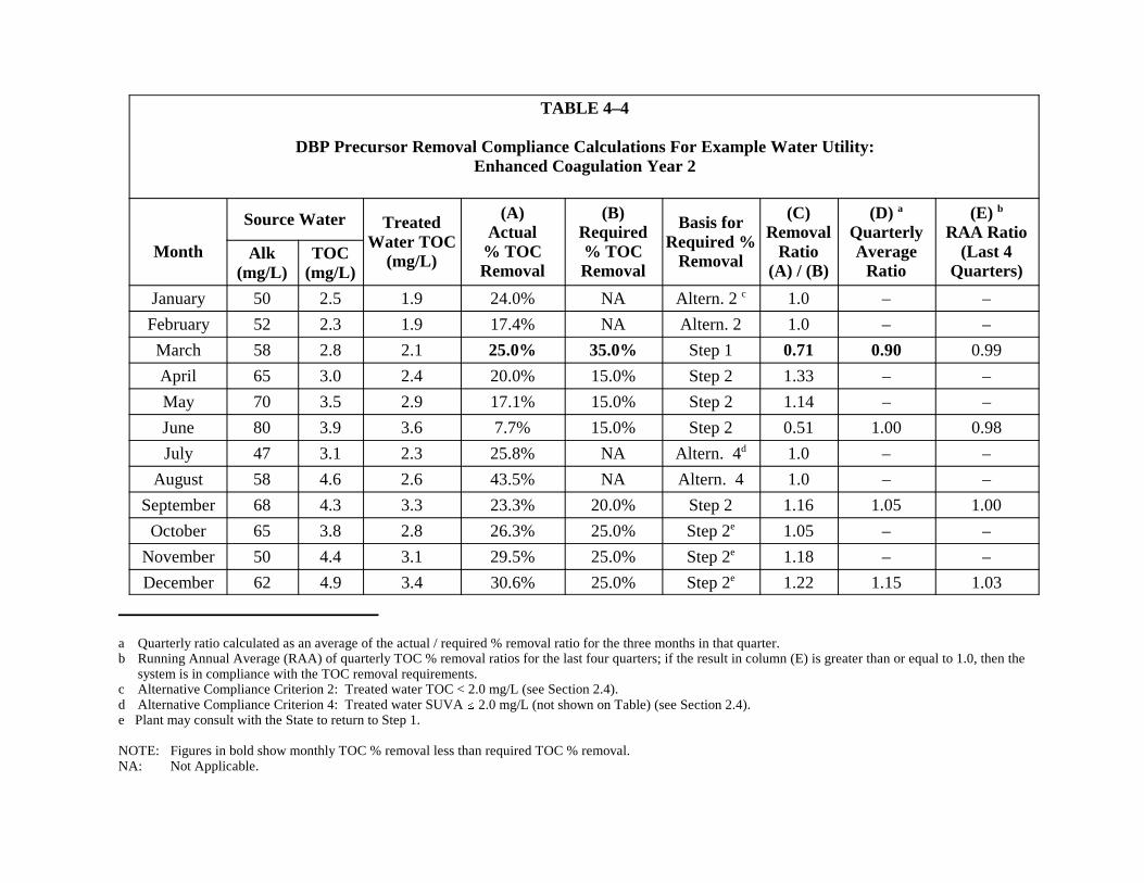
TABLE 4–4

DBP Precursor Removal Compliance Calculations For Example Water Utility:Enhanced Coagulation Year 2

Month


(mg/L)

(A)Actual

% TOCRemoval


Basis forRequired %

Removal

(C)Removal

Ratio(A) / (B)

(D) a

QuarterlyAverage

Ratio

(E) b

RAA Ratio(Last 4

Quarters)Alk

(mg/L)TOC

(mg/L)

January 50 2.5 1.9 24.0% NA Altern. 2 c 1.0 – –

February 52 2.3 1.9 17.4% NA Altern. 2 1.0 – –

March 58 2.8 2.1 25.0% 35.0% Step 1 0.71 0.90 0.99

April 65 3.0 2.4 20.0% 15.0% Step 2 1.33 – –

May 70 3.5 2.9 17.1% 15.0% Step 2 1.14 – –

June 80 3.9 3.6 7.7% 15.0% Step 2 0.51 1.00 0.98

July 47 3.1 2.3 25.8% NA Altern. 4d 1.0 – –

August 58 4.6 2.6 43.5% NA Altern. 4 1.0 – –

September 68 4.3 3.3 23.3% 20.0% Step 2 1.16 1.05 1.00

October 65 3.8 2.8 26.3% 25.0% Step 2e 1.05 – –

November 50 4.4 3.1 29.5% 25.0% Step 2e 1.18 – –

December 62 4.9 3.4 30.6% 25.0% Step 2e 1.22 1.15 1.03

a Quarterly ratio calculated as an average of the actual / required % removal ratio for the three months in that quarter.b Running Annual Average (RAA) of quarterly TOC % removal ratios for the last four quarters; if the result in column (E) is greater than or equal to 1.0, then the

system is in compliance with the TOC removal requirements.c Alternative Compliance Criterion 2: Treated water TOC < 2.0 mg/L (see Section 2.4).d Alternative Compliance Criterion 4: Treated water SUVA � 2.0 mg/L (not shown on Table) (see Section 2.4).e Plant may consult with the State to return to Step 1.


4-16

Example 2 - Enhanced Precipitative Softening

Tables 4-5 and 4-6 show sample running annual average calculations for a softening

plant. In year one (Table 4-5), compliance is based upon achieving a running annual average

of 1.0 or greater after TOC sampling in month 12 is complete (at the end of the fourth

quarter). The monthly removal ratios shown in column C are calculated from the required

Step 1 TOC removal matrix (Table 2-1) and by meeting alternative performance criteria.

Months in which an alternative compliance criterion is used are assigned a monthly removal

ratio of 1.0.

The plant in the example maintains a running annual average greater than 1.0 in year

two and is therefore in compliance. If the plant s running annual average had fallen below

1.0, it would have been out of compliance. It is important that softening plants utilize the

softening-specific alternative compliance criteria discussed in Section 2.4 to maximize their

ability to establish compliance.

TABLE 4–5

DBP Precursor Removal Compliance Calculations for Example Water Utility:Enhanced Precipitative Softening Year 1

Month


(mg/L)

(A)Actual

% TOCRemoval


Basis forRequired %

Removal

(C)Removal

Ratio(A) / (B)

(D) a

QuarterlyAverage

Ratio

(E) b

RAA Ratio(Last 4

Quarters)Alk

(mg/L)TOC

(mg/L)

January 187 3.0 2.1 30.0% 15.0% Step 1 c 2.00 – –

February 180 3.3 2.1 36.4% 15.0% Step 1 2.43 – –

March 195 9.3 5.8 37.6% 30.0% Step 1 1.25 1.89 –

April 200 10.4 6.4 38.5% 30.0% Step 1 1.28 – –

May 208 8.7 5.5 36.8% 30.0% Step 1 1.23 – –

June 212 6.0 4.6 23.3% NA Altern. 2d 1.0 1.17 –

July 220 4.8 3.1 35.4% 25.0% Step 1 1.42 – –

August 218 3.5 2.6 25.7% 15.0% Step 1 1.71 – –

September 206 4.9 3.4 30.6% 25.0% Step 1 1.22 1.45 –

October 196 9.2 6.6 28.3% 30.0% Step 1 0.94 – –

November 190 6.4 5.1 20.3% 25.0% Step 1 0.81 – –

December 182 4.4 3.2 27.3% 25.0% Step 1 1.09 0.95 1.37


system is in compliance with the TOC removal requirements. c Step 1 Required TOC% Removal from Table 2-1 (see Section 2.3.1).d Alternative Compliance Criterion 2 for softening plants: Magnesium hardness removal greater than or equal to 10 mg/L between source water and treated

water (not shown on Table) (see Section 2.4.2).


TABLE 4–6

DBP Precursor Removal Compliance Calculations for Example Water Utility:Enhanced Precipitative Softening Year 2

Month


(mg/L)

(A)Actual

% TOCRemoval


Basis forRequired %

Removal

(C)Removal

Ratio(A) / (B)

(D) a

QuarterlyAverage

Ratio

(E) b

RAA Ratio(Last 4

Quarters)Alk

(mg/L)TOC

(mg/L)

January 185 2.2 1.9 13.6% NA Altern. 1 c 1.0 - -

February 193 3.3 2.2 33.3% 15.0% Step 1 d 2.22 - -

March 197 3.2 2.5 21.9% 15.0% Step 1 1.46 1.56 1.28

April 190 9.6 6.5 32.3% 30.0% Step 1 1.08 - -

May 200 8.4 5.7 32.1% 30.0% Step 1 1.07 - -

June 209 5.7 3.8 33.3% 25.0% Step 1 1.33 1.16 1.28

July 213 4.1 3.1 24.4% NA Altern. 2 e 1.0 - -

August 222 4.4 2.9 34.1% 25.0% Step 1 1.36 - -

September 204 4.3 3.0 30.2% 25.0% Step 1 1.21 1.19 1.22

October 198 8.2 5.6 31.7% 30.0% Step 1 1.06 - -

November 180 7.0 4.9 30.0% 25.0% Step 1 1.20 - -

December 184 4.9 3.3 32.7% 25.0% Step 1 1.31 1.19 1.27


system is in compliance with the TOC removal requirements. c Alternative Compliance Criterion 1: Treated water TOC < 2.0 mg/L (see Section 2.4).d Step 1 Required TOC% Removal from Table 2-1 (see Section 2.3.1).e Alternative Compliance Criterion 2 for softening plants: Magnesium hardness removal greater than or equal to 10 mg/L between source water and treated

water (not shown on Table) (see Section 2.4.2).

NA Not Applicable.

Chapter 5

LABORATORY PROCEDURES

Table of Contents

Page

5.0 LABORATORY PROCEDURES5.1 Introduction . . . . . . . . . . . . . . . . . . . . . . . . . . . . . . . . . . . . . . . . . . . . . 5-15.2 Analytical Methods. . . . . . . . . . . . . . . . . . . . . . . . . . . . . . . . . . . . . . . 5-1

5.2.1 Total Organic Carbon. . . . . . . . . . . . . . . . . . . . . . . . . . . . . . . . 5-25.2.2 Dissolved Organic Carbon. . . . . . . . . . . . . . . . . . . . . . . . . . . . 5-45.2.3 Ultraviolet Light Absorbance at 254 nm. . . . . . . . . . . . . . . . . 5-55.2.4 Specific Ultraviolet Absorption (SUVA). . . . . . . . . . . . . . . . . 5-65.2.5 Alkalinity . . . . . . . . . . . . . . . . . . . . . . . . . . . . . . . . . . . . . . . . . 5-65.2.6 Trihalomethanes. . . . . . . . . . . . . . . . . . . . . . . . . . . . . . . . . . . . 5-75.2.7 Haloacetic Acids. . . . . . . . . . . . . . . . . . . . . . . . . . . . . . . . . . . 5-85.2.8 pH. . . . . . . . . . . . . . . . . . . . . . . . . . . . . . . . . . . . . . . . . . . . . . . 5-95.2.9 Magnesium Hardness. . . . . . . . . . . . . . . . . . . . . . . . . . . . . . . 5-10

5.3 Sample Collection and Handling . . . . . . . . . . . . . . . . . . . . . . . . . . . . 5-115.4 Quality Assurance/Quality Control. . . . . . . . . . . . . . . . . . . . . . . . . . 5-16

5.4.1 Total Organic Carbon. . . . . . . . . . . . . . . . . . . . . . . . . . . . . . . 5-165.4.2 Dissolved Organic Carbon. . . . . . . . . . . . . . . . . . . . . . . . . . . 5-175.4.3 Ultraviolet Absorbance at 254 nm. . . . . . . . . . . . . . . . . . . . . 5-175.4.4 Specific Ultraviolet Absorption. . . . . . . . . . . . . . . . . . . . . . . 5-175.4.5 Alkalinity . . . . . . . . . . . . . . . . . . . . . . . . . . . . . . . . . . . . . . . . 5-185.4.6 Trihalomethanes. . . . . . . . . . . . . . . . . . . . . . . . . . . . . . . . . . . 5-185.4.7 Haloacetic Acids. . . . . . . . . . . . . . . . . . . . . . . . . . . . . . . . . . 5-195.4.8 pH. . . . . . . . . . . . . . . . . . . . . . . . . . . . . . . . . . . . . . . . . . . . . . 5-205.4.9 Magnesium Hardness. . . . . . . . . . . . . . . . . . . . . . . . . . . . . . . 5-20

List of Tables

5-1 Analytical Methods for Demonstration of Compliance. . . . . . . . . . . . . . . . . . 5-25-2 Sample Collection Containers and Preservatives/Dechlorinating Agents . . . . 5-125-3 Sample Handling and Storage . . . . . . . . . . . . . . . . . . . . . . . . . . . . . . . . . . . . . 5-14

5-1

5.0 LABORATORY PROCEDURES

5.1 INTRODUCTION

The water quality parameters that are important for compliance with the treatment

requirement of the DBPR include TOC, alkalinity, pH, TTHM, HAA5, UV-254, DOC,

SUVA, and magnesium hardness. TOC and alkalinity data are needed to demonstrate

compliance with the Step 1 TOC removal requirements (Section 2.3.1). Analysis for pH is

important to ensure that the treatability of samples is examined over an acceptable range of

pH values. TTHM and HAA5 analyses are necessary to qualify for an alternative

compliance criterion (Section 2.4). DOC and UV-254 analyses are used to calculate a

SUVA value which may be needed if alternative compliance criteria are used (Section 2.4).

Magnesium hardness and alkalinity are needed for the alternative compliance criteria for

softening systems (Section 2.4.2). This chapter provides an overview of acceptable

analytical methodologies for each of these water quality parameters. Required procedures

for sample collection, sample handling, and analysis are summarized, along with

recommended quality assurance and quality control practices. The purpose of this chapter

is to provide a general review of laboratory procedures necessary to implement the DBPR,

not to supplant the direction contained in analytical methods required by the DBPR. For

purposes of compliance, the final regulatory language and documents referenced therein

should be used.

5.2 ANALYTICAL METHODS

Only the analytical method(s) specified in the rule, or otherwise approved by the EPA

for monitoring under subpart L section 141.131, may be used to demonstrate compliance

with the enhanced coagulation or enhanced softening requirements of the DBPR. This

chapter is not comprehensive for all water quality parameters and methods required for

compliance with the DBPR. Only those methods necessary for the treatment requirement

of the DBPR are included. Table 5.1 summarizes the analytical methods for the parameters

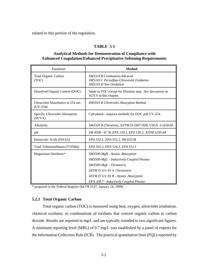
5-2

related to this portion of the regulation.

TABLE 5-1

Analytical Methods for Demonstration of Compliance withEnhanced Coagulation/Enhanced Precipitative Softening Requirements

Parameter Method

Total Organic Carbon(TOC)

SM5310 B Combustion-Infrared SM5310 C Persulfate-Ultraviolet OxidationSM5310 D Wet Oxidation

Dissolved Organic Carbon (DOC) Same as TOC except for filtration step. See discussion onSUVA in this chapter.

Ultraviolet Absorbance at 254 nm(UV-254)

SM5910 B Ultraviolet Absorption Method

Specific Ultraviolet Absorption(SUVA)

Calculated - requires methods for DOC and UV-254.

Alkalinity SM2320 B (Titration), ASTM D-1067-92B, USGS I-1030-85

pH SM 4500 - H +B, EPA 150.1, EPA 150.2, ASTM 1293-84

Haloacetic Acids (HAA5) EPA 552.1, EPA 552.2, SM 6251B

Total Trihalomethanes (TTHMs) EPA 502.2, EPA 524.2, EPA 551.1

Magnesium Hardness* SM3500-MgB - Atomic Absorption

SM3500-MgC - Inductively Coupled Plasma

SM3500-MgE - Titrametric

ASTM D 511-93 A -Titrametric

ASTM D 511-93 B - Atomic Absorption

EPA 200.7 - Inductively Coupled Plasma

* proposed in the Federal Register (64 FR 2537, January 14, 1999)

5.2.1 Total Organic Carbon

Total organic carbon (TOC) is measured using heat, oxygen, ultraviolet irradiation,

chemical oxidants, or combinations of oxidants that convert organic carbon to carbon

dioxide. Results are reported in mg/L and are typically rounded to two significant figures.

A minimum reporting level (MRL) of 0.7 mg/L was established by a panel of experts for

the Information Collection Rule (ICR). The practical quantitation limit (PQL) reported by

5-3

laboratories performing TOC analysis should be consistent with this MRL. Values reported

by the laboratory at less than the PQL should be reported by the plant as half of the PQL.

Three Standard Methods: 5310B, 5310C, and 5310D are included in the DBPR (Table 5-1).

These methods should be followed in accordance with the Supplement to the 19th Edition

of Standard Methods for the Examination of Water and Wastewater, American Public

Health Association, 1998. Method 5310B is a combustion-infrared method; Method 5310C

is a persulfate-ultraviolet oxidation method; and Method 5310D is a wet-oxidation method.

A summary of these methods for the determination of TOC is provided below.

Combustion-Infrared Method (Standard Method 5310B) measures organic carbon

via infrared absorption of the carbon dioxide gas that is produced when the organic carbon

in the sample is heated and reacted with an oxidative catalyst. Inorganic carbon is

converted to CO2 by acidification to pH �2 and is purged from the sample prior to analysis.

This process also removes volatile organic carbon from the sample, which contributes to

carbon loss. However, this loss is generally insignificant. The CO2 from oxidation of

organic and inorganic carbon is measured using a nondispersive infrared analyzer or titrated

colometrically. Any combustion instrument used for compliance purposes under the DBPR

should be capable of providing quantitative data at concentrations �0.5 mg/L.

Persulfate-Ultraviolet Oxidation Method (Standard Method 5310C) measures organic

carbon via infrared absorption of the carbon dioxide gas that is produced when the organic

carbon in the sample is simultaneously oxidized by a persulfate solution and irradiated with

ultraviolet light. Inorganic carbon is converted to CO2 by acidification to pH �2, and is

purged from the sample prior to analysis. Significant concentrations of chloride (�0.1

percent) and a low sample pH (< 1) can impede the analysis; precautions are specified in

the method.

Wet-Oxidation Method (Standard Method 5310D) has a detection limit of 0.10 mg/L,

and is subject to the same interferences as the persulfate-ultraviolet method. Persulfate and

phosphoric acid are added to the sample, and the sample is purged with pure oxygen to

remove inorganic carbon in the form of CO2. The purged sample is sealed in an ampule and

5-4

combusted for four hours at 116-130(C in an oven. This causes the persulfate to oxidize

the organic carbon to CO2. TOC is measured via nondispersive infrared absorption of CO2.

5.2.2 Dissolved Organic Carbon

DOC measurements are performed using the same analytical techniques used to

measure TOC (Combustion-Infrared Method 5310B, Persulfate-Ultraviolet Oxidation

Method 5310C, and Wet Oxidation Method 5310D). However, samples for DOC

measurement must be vacuum-filtered or pressure filtered through a 0.45 µm pore size filter

prior to analysis. Filtering should occur before preservation, storing or shipping the sample.

To ensure sample integrity, no contamination or dilution of the sample during filtration

should occur. To prevent contamination from organic binding material on membrane filters,

the membrane filter must be washed with reagent-grade water. Typically, washing with

several 100 ml volumes of water is required for a 47-mm diameter filter. Vacuum or

pressure filtration can be used to facilitate the process. The laboratory should demonstrate

adequate washing procedures for each batch of filter membranes. EPA suggests that

adequate washing is demonstrated when the DOC of the filtered water is no higher than the

TOC of the water prior to filtration.

Water passed through the filter prior to sample filtration must be saved and used as

a filtered blank. This filtered blank must be analyzed using procedures identical to those

used for analysis of the samples, and must have a DOC content of less than 0.5 mg/L. The

filtration apparatus should be adequately washed to remove organic matter. Highly turbid

samples may require using more than one membrane filter if a filter becomes clogged.

When multiple filter membranes are required for a sample, each filter membrane must be

taken through the same washing procedure as described above, and a filter blank should be

analyzed.

DOC samples must be acidified to a pH of less than 2.0 by adding phosphoric or

sulfuric acid as soon as possible, but not to exceed 48 hours, after sampling and filtration.

Acidified samples must be analyzed within 28 days of sample collection. The DOC of the

5-5

analyzed sample should be less than or equal to the TOC concentration; if not, sample

contamination may have occurred.

5.2.3 Ultraviolet Light Absorbance at 254 nm

Method 5910B should be performed according to Standard Methods for the

Examination of Water and Wastewater, 19th Edition, American Public Health Association,

1998. The principle behind this method is that UV-absorbing constituents will absorb UV

light in proportion to their concentration. UV samples must be measured in waters prior to

the addition of an oxidant or disinfectant. This is necessary because oxidants react with

organic compounds and cleave the double bonds that absorb UV. Samples must be filtered

through a 0.45 )m pore-sized membrane filter. To prevent contamination from organic

material binding on membrane filters, the filters must be washed with reagent-grade water.

Typically, several 100 ml volumes of water are required for a 47-mm diameter filter. UV

absorbance is measured at a wavelength of 253.7 nm (rounded to 254 nm) at ambient pH

using a spectrophotometer. Select sample volume on the basis of the cell path length or

dilution required to produce a UV absorbance between 0.005 and 0.900 cm-1. The

spectrophotometer must be zeroed using an organic-free water blank. UV-254 should be

measured for at least two filtered portions of the sample at room temperature. The average

value is then reported in cm-1 (i.e., the result must be divided by the cell length). UV

measurements are typically made with a 1-cm cell.

A MRL of 0.009 cm-1 was established by a panel of experts for the ICR. It is

recommended that laboratories performing UV254 analysis obtain a PQL of at least 0.009

cm-1. Plants should use half of the PQL for compliance calculations when results are

reported to them by the laboratory as less than the PQL. Samples must be analyzed as soon

as practical, but not to exceed 48 hours, after sampling. The pH of a UV sample may not

be adjusted.

5-6

5.2.4 Specific Ultraviolet Absorption (SUVA)

SUVA at 254 nm is an indicator of the humic content of water (Edzwald and Van

Benschoten, 1990). It is a calculated parameter equal to UV absorption at 254 nm (measured

in m-1) divided by DOC (measured as mg/L). The equation is:

SUVA (L/mg-m) = 100 (cm/m) [UV254 (m-1)/DOC mg/L]

Waters with low SUVA values contain primarily non-humic matter and are not

amenable to enhanced coagulation. SUVA is an alternative compliance criterion for

demonstrating compliance with TOC removal requirements. Systems are not required to

perform enhanced coagulation or enhanced softening if the raw water SUVA is � 2.0 L/mg-

m. Two separate analytical methods are necessary to make this measurement: UV-254 and

DOC. These methods are described in Sections 5.2.2 and 5.2.3. DOC and UV-254 samples

used to determine a SUVA value must be taken at the same time and the same location.

Both samples are filtered according to the procedures outlined in Sections 5.2.2 and 5.2.3.

EPA recommends, but does not require, that both DOC and UV samples be filtered as one

large aliquot.

5.2.5 Alkalinity

Titration methods (Standard Method 2320B, ASTM D1067-92B, or USGS I-1030-85)

are approved for alkalinity measurements at 40 CFR 141.89. Standard Method 2320B can

be found in Standard Methods for the Examination of Water and Wastewater, 19th Edition,

American Public Health Association, 1998. Method ASTM D1067-92B is in the Annual

Book of ASTM Methods, 1998, Vol. 11.01. USGS I-1030-85 can be found in Methods for

Determination of Inorganic Substances in Water and Fluvial Sediments: U.S. Geological

Survey Techniques of Water-Resources Investigations.

Total alkalinity in these methods is measured by titration of the sample to an

electrochemically determined endpoint (e.g., pH 4.5). Alkalinity is reported in milligrams

per liter as calcium carbonate (CaCO3). The methods ascribe the entire alkalinity

concentration to the sum of carbonate, bicarbonate, and hydroxide concentrations, and

5-7

assume an absence of other alkalinity contributing compounds. The measured values may

include contributions from borates, phosphate, silicates, or other bases if these are present

(Standard Methods, 1989, p 2-35).

All procedures and precautions described here and in the methods must be followed

carefully to ensure an accurate measurement of alkalinity. The sample pH of the source

water where the sample was collected must be recorded. Care must be used in sampling and

storage, and in preparation of the primary standards for sodium carbonate, sulfuric acid, and

hydrochloric acid.

5.2.6 Trihalomethanes

EPA Methods 502.2, 524.2, and 551.1 are acceptable for analysis of trihalomethanes.

These methods can be found in Methods for the Determination of Organic Compounds in

Drinking Water - Supplement III, USEPA, August 1995, EPA/600/R-95/131 (available

through NTIS, PB95-262616). The references for methods 502.2 and 524.2 are also

provided in the Federal Register (63 FR 69390, December 16, 1998). The specific reference

for method 551.1 in Supplement III is: Munch, D.J., Hautman, D.P. Method 551.1:

Determination of Chlorination Disinfection Byproducts, Chlorinated Solvents, and

Halogenated Pesticides/Herbicides in Drinking Water by Liquid-Liquid Extraction and Gas

Chromatography with Electron-Capture Detection; Revision 1.0, USEPA, National

Exposure Research Laboratory, Cincinnati, Ohio (1995).

Analyses for TTHMs measure the concentrations of chloroform,

bromodichloromethane, dibromochloromethane, and bromoform. The individual

concentrations of these species are summed together on a mass basis to obtain TTHM. EPA

method 502.2 is a purge and trap gas chromatography (GC) method utilizing an electrolytic

conductivity detector. EPA method 524.2 is a purge and trap gas chromatography/mass

spectrometry method. EPA method 551.1, a GC/electron capture detection method, utilizes

a microextraction technique which allows for the use of pentane or MTBE as the extraction

solvent. This method was developed for the simultaneous analysis of THMs,

haloacetonitriles, haloketones, and chloropicrin. As part of this method, samples are

5-8

preserved with a phosphate buffer that reduces the pH to 5.2, in order to eliminate

degradation of DBPs that can undergo a base-catalyzed hydrolysis. Sodium sulfate is added

to the sample to increase the partitioning of the DBPs from the aqueous phase to the solvent

during the extraction step. The extracts are analyzed by GC with an electron capture detector

(ECD).

Aqueous samples should be extracted for Method 551.1 within two weeks of sample

collection. Extracts can be held for up to two weeks prior to analysis. If transfer of the

samples to other bottles is necessary, pouring should be done slowly to minimize agitation

and contact with the air. However, transfer of the sample to another container is not

recommended. The extraction should be performed in the sample bottle to prevent loss of

chloroform.

5.2.7 Haloacetic Acids

EPA Methods 552.1 and 552.2 are approved methods for the analysis of haloacetic

acids. EPA Method 552.1 can be found in Methods for the Determination of Organic

Compounds in Drinking Water - Supplement II, USEPA, August 1992, EPA/600/R-92/129

(available through NTIS, PB92-207703). EPA Method 552.2 can be found in Methods for

the Determination Organic Compounds in Drinking Water-Supplement III, USEPA, August

1995, EPA/600/R-95/131. The specific reference in Supplement III is: Munch, D.J., J.W.

Munch, and A.W. Pawlecki. Method 552.2: Determination of Haloacetic Acids and Dalapon

in Drinking Water by Liquid-Liquid Extraction, Derivitization and Gas Chromatography

with Electron Capture Detection; revision 1.0, USEPA, National Exposure Research

Laboratory, Cincinnati, Ohio (1995). The micro liquid-liquid extraction gas

chromatographic method (Standard Method 6251 B) is also an acceptable method for HAA5

and can be found in Standard Methods for the Examination of Water and Wastewater, 19th

Edition, American Public Health Association, 1998. Standard Method 6251B was

developed to analyze simultaneously for each of the HAA5 compounds plus 2,3,5-

trichlorophenol. Distribution system samples collected as part of monitoring for an

exemption from the treatment technique for control of disinfection by-product precursors

5-9

should be analyzed for HAA5. The HAA5 list consists of the following five haloacetic

acids: monochloroacetic acid, dichloroacetic acid, trichloroacetic acid, monobromoacetic

acid, and dibromoacetic acid. The ICR required reporting of HAA6, which consists of

HAA5 plus bromochloroacetic acid. Three additional trihalogenated HAAs can now be

detected using Method 552.2, Gas Chromatography/Electron Capture Detection method,

utilizing a microextraction patterned after SM 6251B. This is an improvement over the

solid phase extraction utilized in EPA Method 552.1 which is subject to considerable

variability in sample matrices containing competing ionic species. A Fisher esterification

(an acid-catalyzed reaction of carboxylic acids with alcohols to form esters) is utilized in

method 552.2. A back extraction with saturated sodium bicarbonate is incorporated to

neutralize the acidic extracts and prevent any damage to the GC column. Finally, acidic

methanol derivitization utilized in Method 552.2 provides an alternative to trimethysilyl

diazomethane (TMSD) used in Standard Method 6251B which has carcinogenic and

explosive characteristics. The three additional HAAs are: bromodichloroacetic acid

(BDCAA), chlorodibromoacetic acid (CDBAA) and tribromoacetic acid (TBAA). Analyses

for HAA6 and HAA9 are optional.

5.2.8 pH

Standard Method 4500-H+B, EPA Method 150.1 and 150.2, and ASTM 1293-84 are

acceptable methods for the analysis of pH. Standard Method 4500-H+B can be found in

Standard Methods for the Examination of Water and Wastewater, 19th Edition, American

Public Health Association, 1998. ASTM 1293-84 should be performed according to the

Annual Book of ASTM Methods, 1998, Vol. 11.01. The typical electrometric apparatus (pH

meter) consists of a potentiometer, a glass electrode, a reference electrode, and a

temperature-compensating device. When the electrodes are immersed in the sample

solution, a circuit is completed through the potentiometer; the potentiometer measurement

is used to determine the activity of the hydrogen ions.

5-10

5.2.9 Magnesium Hardness

Precipitative softening systems monitoring to meet alternative performance criteria

(magnesium hardness removal greater than or equal to 10 mg/L as CaCO3) will need to

perform analyses for magnesium. Six magnesium methods have been proposed to

demonstrate compliance with the treatment requirement of the DBPR (64 FR 2537, January

14, 1999). These methods can be grouped into three analytical techniques: (1) atomic

absorption (AA) methods; (2) inductively coupled plasma (ICP) methods; and (3)

complexation titrametric methods.

Atomic Absorption Methods

Method 3500-MgB should be followed as described in Standard Methods for the


1995. ASTM D511-93B should be performed according to the Annual Book of ASTM

Methods, 1998, Vol. 11.01.

In the measurement of magnesium by atomic absorption, a sample is aspirated into

a flame and atomized. The addition of interference-suppressing agents may be necessary.

A light beam is directed through the flame, into a filter or monochromator set at 285.2 nm,

and onto a detector which determines the light absorbed by the magnesium. The

concentration of magnesium is proportional to absorbance within the linear range of the

instrument. These methods are generally applicable to magnesium concentrations in the

range 0.02-3.0 mg/L, depending on the instrument and method employed. Higher

concentrations may be analyzed by dilution of the sample prior to analysis.

Inductively Coupled Plasma Methods

Standard Method 3500-Mg C can be found in Standard Methods for the


1995. EPA Method 200.7 should be performed according to Methods for the Determination

of Metals in Environmental Samples-Supplement I, EPA 600/R-94-111.

5-11

An ICP source consists of a stream of argon gas ionized by an applied radio

frequency field. The field is inductively coupled to the ionized gas by a coil surrounding a

quartz torch that supports and confines the plasma. Analysis of magnesium by ICP involves

generation of a sample aerosol in a nebulizer and subsequent injection into the ICP. This

subjects the constituent atoms to temperatures of 6000 to 8000 (K resulting in almost

complete dissociation of molecules and excitation of atomic emission. A portion of the

emission spectrum (usually 279.08 or 279.55 nm for magnesium) from the ICP is isolated

for intensity measurement. The efficient excitation provided by the ICP results in low

detection limits, and the linear range of the instrument may span four orders of magnitude.

Complexation Titrametric Methods

Standard Method 3500-Mg E can be found in Standard Methods for the


1995. ASTM D 511-93 A can be found in the Annual Book of ASTM Methods, 1998, Vol.

11.01.

The complexation titrametric methods measure magnesium as the difference between

hardness (equal to calcium plus magnesium) and calcium. Hardness is measured by titration

of a sample with EDTA (ethylenediamine tetraacetic acid) at pH 10. Calcium is determined

by titration of a separate aliquot of sample with EDTA at a pH of 12-13, where the

magnesium is precipitated. A chemical indicator is added to the sample to allow

observation of the endpoint. These methods are generally applicable in a range from 1 to

1000mg/l of calcium plus magnesium expressed as calcium, but may fail in the analysis of

highly colored waters that contain high concentrations of metals.

5.3 SAMPLE COLLECTION AND HANDLING

All samples should be collected in accordance with the approved methods. A

summary of various aspects of sample collection and preservation is provided in Tables 5-2

and 5-3.

5-12

TABLE 5-2

Sample Collection Containers and Preservatives/Dechlorinating Agents

PARAMETER METHOD BOTTLE

MATERIAL

CAP/SEPTA

MATERIAL

PRESERVATIVES/

DECHLORINATING AGENTS

Alkalinity SM 2320 B1

ASTM D1067-

92B5

USGS I-1030-856

Polyethylene or

borosilicate glass

(not acid washed)

No

specifications

NONE

Magnesium

Hardness

(Calculation)

SM3500-MgB1

SM3500-MgC2

SM3500-MgE2

ASTM D 511-

93A5

ASTM D 511-

93B5

EPA 200.77

Polypropylene or

liner polyethylene

or borosilicate

glass

Polyethylene

Cap

Acidify with nitric acid (1:1) to pH <2

THM EPA 502.23

EPA 524.23

EPA 551.13

Glass Teflon Lined

Septa

For 502.2 & 524.2: add 3 mg

Na2S2O3/40 ml sample or 3 mg

Na2S2O3/40 ml sample and

acidification using HCl to pH < 2.0 or

25 mg ascorbic acid/40 ml sample and

immediate acidification using HCl to

pH<2. Note: Samples must be

dechlorinated prior to acidification).

For method 551.1 preserve and

dechlorinate using 1g phosphate

buffer* and NH4Cl or Na2SO3

mixture/60 ml sample (mixture consist

of 1 part Na2HPO4, 99 parts KH2PO4

and 0.6 parts NH4Cl or Na2SO3. 1 g per

60 ml results in a pH of 4.5 - 5.5 and

0.1 mg NH4Cl or Na2SO3 per ml of

sample.

* 2 g phosphate buffer may be needed

TOC SM 5310 B1

SM 5310 C1

SM 5310 D1

Amber Glass Teflon Lined

Septa

Adjust to pH <2 using phosphoric or

sulfuric acid (or alternate acid if

recommended by the instrument

manufacturer)

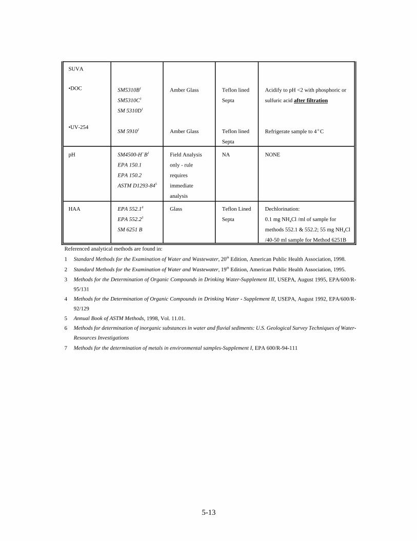
5-13

SUVA

•DOC

•UV-254

SM5310B1

SM5310C1

SM 5310D1

SM 59101

Amber Glass

Amber Glass

Teflon lined

Septa

Teflon lined

Septa

Acidify to pH <2 with phosphoric or

sulfuric acid after filtration

Refrigerate sample to 4 o C

pH SM4500-H+B1

EPA 150.1

EPA 150.2

ASTM D1293-845

Field Analysis

only - rule

requires

immediate

analysis

NA NONE

HAA EPA 552.14

EPA 552.23

SM 6251 B

Glass Teflon Lined

Septa

Dechlorination:

0.1 mg NH4Cl /ml of sample for

methods 552.1 & 552.2; 55 mg NH4Cl

/40-50 ml sample for Method 6251B

Referenced analytical methods are found in:

1 Standard Methods for the Examination of Water and Wastewater, 20th Edition, American Public Health Association, 1998.

2 Standard Methods for the Examination of Water and Wastewater, 19th Edition, American Public Health Association, 1995.

3 Methods for the Determination of Organic Compounds in Drinking Water-Supplement III, USEPA, August 1995, EPA/600/R-

95/131

4 Methods for the Determination of Organic Compounds in Drinking Water - Supplement II, USEPA, August 1992, EPA/600/R-

92/129

5 Annual Book of ASTM Methods, 1998, Vol. 11.01.

6 Methods for determination of inorganic substances in water and fluvial sediments: U.S. Geological Survey Techniques of Water-

Resources Investigations

7 Methods for the determination of metals in environmental samples-Supplement I, EPA 600/R-94-111

5-14

TABLE 5-3

Sample Handling and Storage

PARAMETER METHOD STORAGE

TEMP

MAX HOLD

TIME

SPECIAL SAMPLE COLLECTION

GUIDELINES

Alkalinity SM 2320 B1

ASTM D 1067-92B5

USGS I - 1030 -

856

(preferred)

Keep at 4°C

ASAP not to

exceed 14

days

Fill bottle completely and cap tightly.

Avoid sample agitation and prolonged

exposure to air. A minimum sample

size of 200 mL is recommended for a

single alkalinity analysis. The sample

pH at the source where the sample is

collected must be recorded.

Magnesium

Hardness

SM3500-MgB1

SM3500-MgC2

SM3500-MgE2

ASTM D 511-93 A5

ASTM D 511-93 B5

EPA 200.77

Keep at 4°C 6 months A volume of at least 500 ml is

recommended.

pH SM 4500-H+

B1

EPA 150.1

EPA 150.2

ASTM D1293-845

NA Field

Analysis

None Specified

TOC SM 5310 B1

SM 5310 C1

SM 5310 D1

Keep at 4°C 28 Days Fill bottle but do not overflow and

flush out preservatives. No air bubbles.

Sample must be headspace free. A

minimum of 100 mL should be taken.

SUVA

•DOC

•UV-254

SM 5310 B1

SM 5310 C1

SM 5310 D1

SM 59101

Keep at 4°C

Keep at 4°C

28 Days

ASAP; not to

exceed 48

hours

1. Fill bottles

2. Filter ASAP (not to exceed 48 hrs)

3. Acidify DOC to pH < 2.0

Note: Add preservative to DOC sample

after filtration.

Refrigerate the UV 254 sample for

preservation.

5-15

TABLE 5-3 (cont.)

Sample Handling and Storage

PARAMETER METHOD STORAGE

TEMP

MAX HOLD

TIME

SPECIAL SAMPLE COLLECTION

GUIDELINES

THM EPA 502.23

EPA 524.23

EPA 551.13

Keep at 4°C 14 days Fill bottle but do not overflow, do not

flush out preservatives and place on a

level surface; the TFE side of the

septum seal should then be slid across

the convex meniscus of the sample, and

the lid screwed on tightly. No air

bubbles. Sample must be headspace

free. Bottles must have a capacity of at

least 50 mL.

HAA EPA 552.14

EPA 552.23

SM 6251B

Keep at 4°C 14 days Fill bottle but do not overflow, do not

flush out preservatives. No air bubbles.

Samples should be headspace free.

Bottles must have a capacity of at least

50 mL.

Referenced analytical methods are found in:1 Standard Methods for the Examination of Water and Wastewater, 20th Edition, American Public Health Association, 1998. 2 Standard Methods for the Examination of Water and Wastewater, 19th Edition, American Public Health Association, 1995. 3 Methods for the Determination of Organic Compounds in Drinking Water-Supplement III, USEPA, August 1995, EPA/600/R-

95/1314 Methods for the Determination of Organic Compounds in Drinking Water - Supplement II, USEPA, August 1992, EPA/600/R-

92/1295 Annual Book of ASTM Methods, 1998, Vol. 11.01. 6 Methods for determination of inorganic substances in water and fluvial sediments: U.S. Geological Survey Techniques of Water-

Resources Investigations7 Methods for the determination of metals in environmental samples-Supplement I, EPA 600/R-94-111

5-16

5.4 QUALITY ASSURANCE/QUALITY CONTROL

Quality Assurance/Quality Control (QA/QC) should follow the practices in the

approved methods described in the previous sections, or other practices approved by the

EPA for each of the methods found in Table 5-1. Other suggested QA/QC practices and

highlights from the methods are summarized in the following subsections.

5.4.1 Total Organic Carbon

Analyses under this section must be conducted by a laboratory approved by the State

or EPA. The QA program should include analysis of replicate samples for precision and

of spiked samples for accuracy. Spiked samples are those to which a known amount of

organic carbon has been added and are used to indicate the degree to which the sample

matrix impacts analytical accuracy. The laboratory should analyze blanks to demonstrate

that interferences from background contamination do not occur. Measurements of spikes,

blanks, and replicate samples should be recorded and reported by the laboratory performing

the analyses. The calibration curves should be linear and should bracket both the low and

high end of the concentration levels to be reported. If the TOC level exceeds the highest

calibration standard, the sample can be diluted into the calibration range with organic-free

water. If the TOC level is below the lowest standard, then TOC should not be quantified.

The lowest standard should represent the lowest TOC concentration that is quantitated (i.e.,

the minimum reporting level).

PE samples may be obtained from a commercial PE provider approved by the

National Institute of Sciences and Technology (NIST). TOC samples are provided in the

wastewater PE studies and may eventually be provided in the drinking water PE studies.

Samples should be precise to at least a two percent relative standard deviation (up to a

maximum of 0.2 mg/L TOC), or to 0.05 mg/L, whichever is larger.

5-17

5.4.2 Dissolved Organic Carbon

The QA program for DOC measurements should include those QA/QC guidelines

described for TOC analysis. The analyst should take great care to ensure that the filtration

step does not result in a loss or gain of DOC. As stated above, DOC can be altered during

the filtration process both by desorption of organic material from the filter into the sample

and by adsorption of DOC from the sample onto the filter. The contribution of filters to

DOC must be checked by analyzing a filtered blank, and the contact of the sample with

organic material, such as contaminated glassware, plastic ontainers, and rubber tubing,

should be avoided as this may contaminate the sample.

5.4.3 Ultraviolet Absorbance at 254 nm

The QA program should include replicate sample analyses. At least two portions of

each sample should be tested. After every tenth sample a duplicate analysis should be

performed to assess analytical precision by repeating the entire sample preparation and

testing process. The baseline absorbance for the spectrophotometer should be checked after

every ten samples by testing the absorbance of organic-free water. A non-zero reading may

indicate the need for cell cleaning, a problem with the reference cell, or a fluctuating

spectrophotometer response caused by heating or power fluctuations. Spectrophotometer

performance can be verified as described in Standard Method 5910B. The same filtration

requirements as for DOC should be repeated and the filter blanks should be < 0.0045 cm-1.

5.4.4 Specific Ultraviolet Absorption

If the DOC measured for a sample is greater than the TOC, sample contamination has

occurred due either to the filter or to an alternate carbon source like contaminated glassware,

rubber tubing, or plastic containers. Filters should be evaluated by analyzing filtrate (in a

fresh flask) from an aliquot of organic-free water. If the filter washing step was adequate,

a post-wash filtrate with organic-free water should be free of DOC. Some brands of 0.45

µm filter paper have surfactant in them which facilitates filtration of microbial samples but

are difficult to wash. Filters with surfactants or those made of cellulose acetate should be

avoided.

5-18

Because disinfectants/oxidants (chlorine, ozone, chlorine dioxide, potassium

permanganate) can degrade UV absorbing compounds without affecting the DOC

concentration, SUVA should be determined on water prior to the application of

disinfectants/oxidants. If disinfectants/oxidants are applied in raw water transmission lines

upstream of the plant, the raw water SUVA determination should be based on a sample

collected upstream of the point of disinfectant/oxidant addition. If the plant applies

disinfectants/oxidants prior to the settled water sample tap, settled water SUVA

measurements should be obtained from jar tests. Finally, the use of iron-based coagulants

can interfere with UV measurements, since dissolved iron can penetrate the filter paper. To

determine settled water SUVA, jar tests with aluminum-based coagulants, and not iron-

based coagulants, should be performed.

5.4.5 Alkalinity

The QA program should include replicate sample analysis for precision. Two

important items affecting the accuracy of the alkalinity method are reagent preparation and

meter calibration. Procedures for standardization of the reagents are specified in the

titration method and should be followed. Both the pH meter and the potentiometer should

be calibrated just prior to the analysis.

5.4.6 Trihalomethanes

The QA program should include replicate sample analysis for precision, and spiked

samples for accuracy. The laboratory should analyze blanks to demonstrate that

interferences from background contamination do not occur. If THMs are not routinely

found in samples, replicate spiked samples should be run periodically to develop precision

THM data. Measurements of spikes, blanks, and replicate samples should be recorded and

reported by the laboratory performing the analyses. The calibration curve should have

sufficient points to describe the shape of the curve, and the curve should bracket both the

low and high ends of the concentration levels to be reported. If the THM level exceeds the

highest calibration standard, the extract can be diluted into the calibration range and re-

injected into the GC. If the THM level is below the lowest standard, then THM levels

5-19

should not be quantified. A PE standard is available for THMs, and procedural standards

should be run.

Each sample should be quenched according to the instructions in Table 5-2 at the

time of sample collection to halt additional production of THMs during the sample holding

time. The quenching converts free chlorine residual to chloramines. Chloramines will not

react with natural organic matter (NOM) to form THMs if the sample is kept at 4(C and the

two-week holding time is not violated. Finally, the solvent used for the extraction should

be free of THMs.

5.4.7 Haloacetic Acids

The QA program should include replicate sample analysis for precision, and spiked

samples for accuracy. The laboratory should analyze blanks to demonstrate that

interferences from background contamination do not occur. If HAAs are not routinely

found in samples, replicate spiked samples should be run periodically to develop precision

HAA data. Measurements of spikes, blanks, and replicate samples should be recorded and

reported by the laboratory performing the analyses. The calibration curve should have

sufficient points to describe the shape of the curve, and the curve should bracket both the

low and high ends of the concentration levels to be reported. If the HAA level exceeds the

highest calibration standard, the extract can be diluted into the calibration range and re-

injected into the GC. If the HAA level is below the lowest standard, then HAA levels

should not be quantified, since the shape of the curve is not always linear to "zero."

Commercially available PE standards are available for HAAs. The PE standards may

include some chlorinated phenols. Chlorinated phenols are not subject to this requirement,

so acceptable performance for the PE standards will only be based on the HAAs.

5-20

5.4.8 pH

The QA program should include replicate sample analysis for precision. Storage and

preparation of the electrodes should be in accordance with the manufacturer’s instructions.

The electrode system should be calibrated against standard buffer solutions of known pH.

When taking a measurement, gently stir the sample to insure homogeneity and to establish

equilibrium between electrodes.

5.4.9 Magnesium Hardness

When performing the magnesium methods, the QA program should include replicate

sample analysis for precision. Select a sample volume that requires less than 15 ml EDTA

titrate. Typical sample volumes are 25 to 50 ml. For low-hardness waters (<5 mg/L), take

a larger sample volume (Standard Methods, 1989, pp. 2-54).

Additional QA items when performing the atomic absorption methods include the

analysis of a blank between samples, and standard readings to verify baseline stability. A

known amount of metal should be added to one out of every ten samples, then analyzed to

confirm recovery. A standard solution also should be measured for every ten samples in

order to assure that the test is in control.

Chapter 6

SECONDARY EFFECTS OF ENHANCED COAGULATIONAND ENHANCED PRECIPITATIVE SOFTENING


6.0 SECONDARY EFFECTS OF ENHANCED COAGULATION AND ENHANCEDPRECIPITATIVE SOFTENING6.1 Introduction . . . . . . . . . . . . . . . . . . . . . . . . . . . . . . . . . . . . . . . . . . . . . . . . . . . . 6-16.2 Evaluation and Implementation . . . . . . . . . . . . . . . . . . . . . . . . . . . . . . . . . . . . . 6-16.3 Inorganic Contaminants . . . . . . . . . . . . . . . . . . . . . . . . . . . . . . . . . . . . . . . . . . . 6-2

6.3.1 Manganese. . . . . . . . . . . . . . . . . . . . . . . . . . . . . . . . . . . . . . . . . . . . . . . 6-36.3.2 Aluminum . . . . . . . . . . . . . . . . . . . . . . . . . . . . . . . . . . . . . . . . . . . . . . . 6-76.3.3 Sulfate/Chloride/Sodium/Iron. . . . . . . . . . . . . . . . . . . . . . . . . . . . . . . 6-11

6.4 Corrosion Control . . . . . . . . . . . . . . . . . . . . . . . . . . . . . . . . . . . . . . . . . . . . . . 6-126.5 Primary Disinfection . . . . . . . . . . . . . . . . . . . . . . . . . . . . . . . . . . . . . . . . . . . . 6-17

6.5.1 Chlorine. . . . . . . . . . . . . . . . . . . . . . . . . . . . . . . . . . . . . . . . . . . . . . . . 6-176.5.2 Ozone. . . . . . . . . . . . . . . . . . . . . . . . . . . . . . . . . . . . . . . . . . . . . . . . . . 6-186.5.3 Chloramine. . . . . . . . . . . . . . . . . . . . . . . . . . . . . . . . . . . . . . . . . . . . . . 6-196.5.4 Chlorine Dioxide. . . . . . . . . . . . . . . . . . . . . . . . . . . . . . . . . . . . . . . . . 6-20

6.6 Particle and Pathogen Removal . . . . . . . . . . . . . . . . . . . . . . . . . . . . . . . . . . . . 6-206.7 Residuals Handling, Treatment, and Disposal . . . . . . . . . . . . . . . . . . . . . . . . . 6-23

6.7.1 Increased Quantity of Sludge. . . . . . . . . . . . . . . . . . . . . . . . . . . . . . . . 6-246.7.2 Altered Characteristics of Sludge. . . . . . . . . . . . . . . . . . . . . . . . . . . . 6-29

6.8 Operation and Maintenance . . . . . . . . . . . . . . . . . . . . . . . . . . . . . . . . . . . . . . . 6-336.9 Recycle Streams . . . . . . . . . . . . . . . . . . . . . . . . . . . . . . . . . . . . . . . . . . . . . . . . 6-34

List of Tables

6-1 Disinfectant Effectiveness under Typical Operating Conditions. . . . . . . . . . . . . . . . . 6-17

List of Figures

6-1 Flowchart for Development of Manganese Removal Strategy with EnhancedCoagulation . . . . . . . . . . . . . . . . . . . . . . . . . . . . . . . . . . . . . . . . . . . . . . . . . . . . . . . . . . 6-8

6-2 Flowchart for Development of Mitigation Strategy for Aluminum Carryover. . . . . . 6-106-3 Effect of Change of Various Water Quality Parameters due to Enhanced

Coagulation on Corrosion of Various Piping Materials . . . . . . . . . . . . . . . . . . . . . . . . 6-136-4 Effect of Change of Various Water Quality Parameters due to Enhanced

Softening on Corrosion of Various Piping Materials . . . . . . . . . . . . . . . . . . . . . . . . . . 6-146-5 Flowchart for Developing a Mitigation Strategy for Corrosion Control. . . . . . . . . . . 6-166-6 Flowchart for Developing a Mitigation Strategy for Particle Removal

Problems due to Enhanced Coagulation or Softening . . . . . . . . . . . . . . . . . . . . . . . . . 6-226-7 Impact Determination of Increased Sludge Volume . . . . . . . . . . . . . . . . . . . . . . . . . . 6-276-8 Mitigation of Impacts from Changes in Sludge Characteristics. . . . . . . . . . . . . . . . . 6-32

6-1

6.0 SECONDARY EFFECTS OF ENHANCED COAGULATIONAND ENHANCED PRECIPITATIVE SOFTENING

6.1 INTRODUCTION

The implementation of enhanced coagulation or enhanced softening may require

process modifications for some utilities. The process modification could have secondary

effects, some of which are expected to be beneficial (e.g., improved disinfection at lower

pH), while others could be detrimental (e.g., production of larger sludge quantities). Most

systems should be able to implement enhanced coagulation or enhanced softening with

minimal secondary effects. This chapter provides guidance to systems that experience

secondary effects to help them mitigate their occurrence and severity. A clear understanding

of potential secondary effects and adequate planning to develop mitigation strategies is

important to minimize the impact of secondary effects the plants may experience while

implementing the treatment technique.

6.2 EVALUATION AND IMPLEMENTATION

Problems related to the implementation of enhanced coagulation or enhanced

softening can be reduced if the affected process has been evaluated with potential secondary

effects in mind. In many cases, bench- or pilot-scale testing can be conducted before

enhanced coagulation or enhanced softening is implemented to completely characterize the

secondary effect and to develop a mitigation strategy. The bench- or pilot-scale study should

be well planned prior to beginning any tests. A comprehensive test plan should be prepared.

The test plan should consider all aspects of the process in question including corrosion,

particle removal, metals removal, disinfection and disinfection byproducts, and other site-

specific concerns.

6-2

Testing should follow a sequence of increasing complexity to screen out variables

that may not be the source of the problem. A test plan may have the following sequential

components:

• Desktop study (review of existing data and literature)

• Jar testing

• Pilot testing

• Partial or full-scale demonstration

Utilities should consider site-specific needs when developing a test plan. Changes in

water quality characteristics that result from a process change can be determined by

comparing the test results for the new conditions with test results simulating existing

conditions. Testing should be calibrated to simulate existing full-scale conditions. These

comparisons will help estimate the type and magnitude of any expected changes due to

enhanced coagulation and softening.

Implementation of the process change may proceed if the test plan results indicate the

change will be successful. The highest risk to operational success and water quality will

occur during initial full-scale operational changeover. Careful planning and extended

monitoring should be practiced to minimize risk and detect any short- or long-term impacts.

An operations plan and a thorough monitoring plan should be developed for the change.

Operational changes should be made during a non-critical treatment period (e.g., warm water

or low demand). Experience should be gained operating under the new conditions when

operations are stable and the water quality is relatively constant. Implementing operational

changes during low flow periods will allow operators to reduce loading rates and compensate

for possible problems in process control.

6.3 INORGANIC CONTAMINANTS

Enhanced coagulation or softening can affect the control of inorganic contaminants,

including iron, manganese, aluminum, sulfate, chloride, and sodium. Maximum contaminant

levels (MCLs) do not currently exist for these contaminants. A secondary maximum

6-3

contaminant level (SMCL) is currently in effect for manganese, aluminum, iron, and

chloride. In addition, some states regulate sodium as a contaminant. The following

subsections provide guidance on techniques applicable to maintaining existing levels of these

contaminants in finished water under enhanced coagulation or enhanced softening

operations.

6.3.1 Manganese

Manganese, even at levels well below the SMCL of 0.05 mg/L, causes discolored

water and can prompt customer complaints. Also, once manganese settles out in the

distribution system, it is difficult to remove and can lead to severe discoloration problems

during significant increases in flow (e.g., fire fighting efforts and main breaks). Manganese

is typically removed from raw water using direct oxidation/coagulation/filtration or filter

adsorption/oxidation (i.e., green sand).

The direct oxidation process uses an oxidant to transform manganese from a

dissolved state (Mn+2) to a solid (MnO2) that can be removed during sedimentation and

filtration (Knocke et al., 1990a). The filter adsorption process occurs when the filter medium

is coated with manganese oxide (i.e., green sand). The Mn+2 adsorbs to the oxide surface and

regenerates the sorption site upon oxidation. Chlorine is usually used for oxidation. Both of

these manganese removal processes can be impacted by enhanced coagulation.

Characteristics of the potential impacts to manganese removal processes are described below.

Slower oxidation at lower coagulation pH

A low pH hinders the direct oxidation process because the oxidation rate of

manganese increases as pH increases. Enhanced coagulation will increase metal salt

coagulant dose and suppress the pH; therefore, slower rates of oxidation can be expected. If

the manganese is being completely oxidized before the coagulation process, however,

enhanced coagulation should not have an impact on the oxidation process. If manganese is

oxidized after the coagulation process (e.g., intermediate ozonation), pH depression can

affect the efficiency of the removal process.

6-4

When manganese is removed with chlorine (Cl2), the oxidation can be relatively slow

(15 minutes to greater than 4 hours), and there may be insufficient contact time before

coagulation for complete oxidation. If potassium permanganate (KMnO4), chlorine dioxide

(ClO2), or ozone (O3) is applied before coagulation, the oxidation rate is fast enough that

complete reaction can occur in the contact time available before coagulation (typically less

than 5 minutes), even at pH values as low as 4.5 (Knocke and Van Benschoten, 1989). The

impact of enhanced coagulation on manganese removal efficiency will be greatest when Cl2

is used with a high rate process (e.g., plate settling) that provides less than two hours of

contact time between the coagulation and filtration processes.

The manganese removal efficiency of the filter adsorption/oxidation process is

reduced when the filter influent pH is below approximately 6.2. The reduction in efficiency

is probably due to the lower oxidation rate of the sorbed Mn+2 ions, i.e., the lower pH reduces

the oxidation rate, and the regeneration of surface adsorption sites (MnO2 surfaces) is not

occurring fast enough to prevent dissolved manganese from passing through the filters into

the finished water. The pH at which the filter adsorption/oxidation process becomes less

effective will vary depending on the pre-filter chlorine dose, the filter loading rate, the filter

media configuration, and the overall water quality.

Manganese contamination of ferric salts

Another impact of enhanced coagulation on the manganese removal process is the

relatively high concentration of this element typically found in ferric chloride and ferric

sulfate. If a utility switches from low doses of ferric or alum to high doses of ferric, the

coagulant itself may significantly increase the amount of dissolved manganese added to the

water stream.

Mitigation Strategies

The flowchart shown in Figure 6-1 describes the potential mitigation strategy for

manganese removal problems due to the implementation of enhanced coagulation. As with

all secondary effects, characterization studies should be conducted before proceeding with

the development of mitigation strategies.

6-5

There are three fractions of manganese that are important for drinking water

treatment; dissolved, colloidal, and particulate. Dissolved manganese can be either Mn+2 or

MnO4-. Colloidal manganese is MnO2 that has not coagulated to a particulate size.

Procedures for determining the fractionation of manganese have been described by Carlson et

al. (1997). Manganese fractionation should be determined in the raw water, after pre-

oxidation, after rapid mix, before the filters, and after the filters. The fractionation data allow

the utility to determine whether a manganese removal problem is due to the direct oxidation

process, the filter adsorption/oxidation process or ferric coagulant addition.

Based on the results of the characterization, one of the three flowchart branches in

Figure 6-1 should be used to develop a mitigation strategy. If the problem appears to be the

direct oxidation process, four modifications should be evaluated:

1) increasing the contact time for oxidation before coagulant addition

2) increasing the oxidant dose

3) increasing the pH during oxidation and then decreasing the pH for coagulation

4) changing the oxidant type to complete the reaction before coagulation

The oxidant contact time may be increased by moving the oxidant addition point as

far upstream as possible. A detention basin could be built to provide contact time prior to

coagulation, but this may be costly. When the oxidant dose is increased, the oxidation rate

increases, and less contact time will be needed before coagulation. There may be limits on

how much the dose can be increased due to disinfection byproduct formation, or concern

regarding residual oxidant reaching the filters. Increasing the pH for oxidation, followed by

acid addition for coagulation, may increase the oxidation rate to an acceptable level.

However, it may require an extensive chemical feed system. In some cases, it may make

sense to switch to a stronger oxidant that can oxidize the manganese within the available

contact time. For example, chlorine dioxide could be used instead of KMnO4 and the capital

investment required may be small. However, ClO2 byproducts and an increase in operating

costs can be expected.

6-6

The feasibility and cost of each of these process modifications will be site-specific;

therefore, a general cost quantification cannot be provided. If these modifications do not

provide acceptable manganese removal, the filter adsorption/oxidation process should be

used in addition to the direct oxidation process. The filters may need to be seeded with

manganese oxide to initiate this process as described by Knocke et al. (1990b) and Merkle et

al. (1997).

If the characterization indicates the utility has a problem with the filter

adsorption/oxidation process, the chlorine dose applied to the filter influent should be

increased. An increased dose will increase the oxidation rate and may offset the decrease in

pH caused by enhanced coagulation. If an increased chlorine dose does not provide

acceptable manganese removal it may be necessary to increase the pH before filtration. The

pH should be increased to the minimum value that will yield acceptable manganese removal

without producing excessive soluble aluminum (see Section 6.3.2). Also, particle removal

may decrease and cause this alternative to be an unacceptable mitigation measure.

When the manganese removal problem is due to contaminated ferric salt, the first

remediation step should be to optimize the procurement purity specification. The maximum

acceptable contribution of manganese from the ferric coagulant should be calculated based

on the anticipated maximum coagulant dose, raw water manganese concentrations, and the

utility’s finished water manganese goals. If the required purity cannot be achieved, the utility

should consider switching to an alternative coagulant (e.g., alum) that is not contaminated

with manganese. If an alternative coagulant is not feasible, the utility should pursue

optimization of the filter adsorption/oxidation process to remove the manganese added with

the ferric coagulant.

The flowchart in Figure 6-1 should help utilities develop an acceptable mitigation

strategy. If the manganese concentration in the finished water is still not acceptable after

implementation of the process modifications, additional characterization studies should be

conducted. This should rarely occur, and when it does occur, it will most likely be due to

inadequate initial characterization studies.

Pre-ozonation can complicate the removal of manganese with or without enhanced

coagulation. Removal of manganese before ozonation prevents the formation of the soluble

6-7

MnO4- ion. Mixed results have been reported on the effectiveness of pre-ozonation for

manganese removal, and pilot testing is recommended before this strategy is chosen.

Cost Implications

The cost impact associated with mitigating these secondary impacts can vary widely.

Minor cost increases can result from a change in the chemical quantities added to the process.

Moderate costs can be incurred if new chemical facilities are required. Higher costs may be

incurred if there is a requirement for new detention facilities or major changes in oxidants or

other chemical systems.

6.3.2 Aluminum

Aluminum can pass through the filters and cause several problems in the distribution

system. For example, when soluble aluminum precipitates after filtration, the turbidity of the

water can increase and “dirty water” complaints from customers may result. Also, aluminum

deposition in the distribution system can lead to reduced hydraulic capacity due to friction

and the thickness of the aluminum films (Kriewall, 1996). Aluminum is also frequently

found in deposits in transmission mains and service lines and has shown some tendency to

function as a film that reduces the leaching of metals into the water (Fuge et al., 1992; Lauer

and Lohman, 1994). The secondary maximum contaminant level (SMCL) for aluminum was

promulgated on January 30, 1991 at 0.05 to 0.2 mg/L to prevent postprecipitation of

aluminum and discoloration of drinking water in distribution systems (Federal Register, 56

FR 3526, January 30, 1991). Aluminum is typically controlled in drinking water by 1)

lowering solubility by controlling pH prior to filters, 2) optimizing the filtration process,

and 3) minimizing aluminum contamination from downstream lime sources. Potential

impacts to these process operations are presented below.

Aluminum solubility at low pH

The minimum solubility of aluminum occurs at a pH of 6.2 to 6.5. Utilities operating

at a pH of less than 6.0 that do not increase the pH before filtration may be impacted the most

due to the solubility of aluminum at this pH. Aluminum solubility also increases significantly

above a pH of 8.0. If a utility practices enhanced softening and does not adjust pH before

filtration, aluminum carryover problems may result.

Characterize Problem - Mn Fractionation - Establish goals

Mn concentrationsacceptable?

No ActionYes

Optimize directoxidation process - pH - oxidant dose - contact time - oxidant type

Optimize ferric coagulant purity specification




Optimize filter adsorption/oxidation process - Cl2 dose - pH

Direct oxidationproblem No

Ferric contaminationproblem

Filter adsorption/oxidation problem

Alternativecoagulant

acceptable?

No ActionYes

No ActionYes

Perform furthercharacterization studies

No Action

No

YesYes

No

No

No

Figure 6-1. Flowchart for developmentof manganese removal strategywith enhanced coagulation.

6-9

Presence of colloidal aluminum hydroxide at high alum doses

Colloidal aluminum can pass through filter processes that have not been optimized.

This fraction of aluminum may not show up as turbidity and can cause distribution system

problems. If a utility currently allows colloidal aluminum to pass through its filters, the

implementation of enhanced coagulation can make the problem worse.

Aluminum contamination of lime

Lime can be contaminated with soluble aluminum. Significant amounts of aluminum

can be added to the water at high lime doses. If lime is added before filtration and the pH is

uncontrolled, soluble aluminum can pass through the filters. If lime is added after the filters,

the aluminum contaminant will pass directly into the distribution system.


The flowchart shown in Figure 6-2 assists in the selection of a mitigation strategy for

aluminum carryover. If a problem with aluminum carryover is suspected, characterization

studies similar to those described for manganese removal should be conducted. Since

aluminum is not currently regulated for health effects (i.e., a MCL), the utility should

establish a finished water goal based on customer expectations before beginning remediation

actions. Also, a baseline of aluminum concentration should be established to assist in

assessing the impact of any future regulation.

In the case of aluminum, particulate and soluble fractions can be determined as

described by Teefy et al. (1992). The soluble and particulate (including colloidal) fractions

should be determined at the raw water, post-filtration, post-lime addition, and pre-filtration

stages. The characterization results will indicate which of three potential aluminum

carryover mechanisms are contributing to the problem. If soluble aluminum is passing

through the filters, the pH of the filter influent should be optimized. This can be

accomplished by adding base to bring the pH up to the minimum solubility level of

aluminum (6.2 - 6.8), but not significantly higher. Any adverse impact to particle removal

should be monitored.

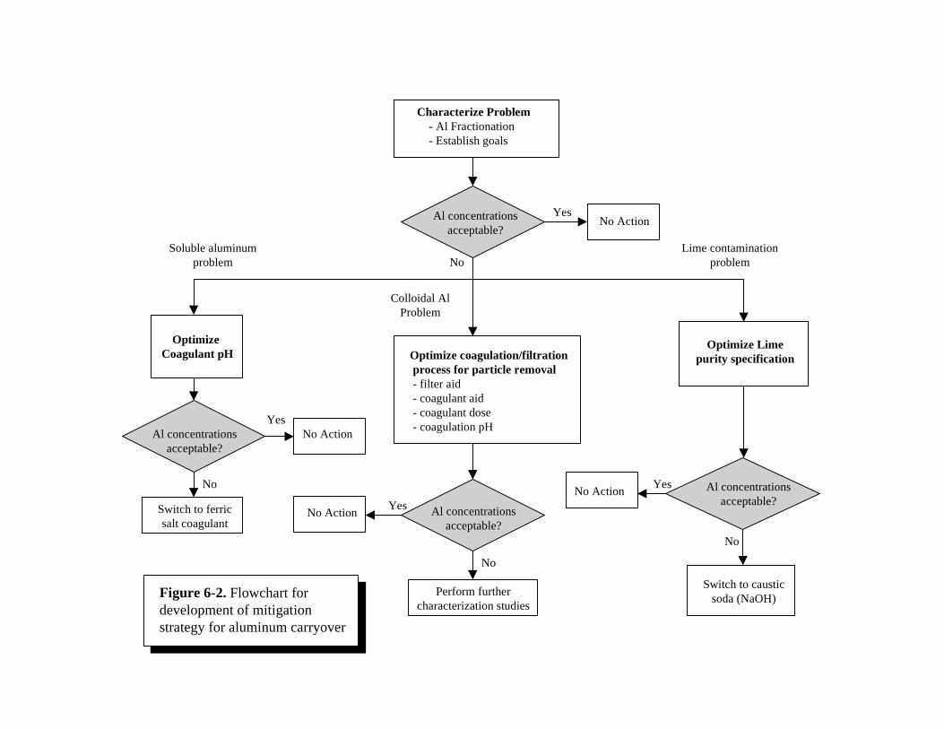
Characterize Problem - Al Fractionation - Establish goals

Al concentrationsacceptable?

No ActionYes

Optimize Coagulant pH

Optimize Limepurity specification




Optimize coagulation/filtration process for particle removal - filter aid - coagulant aid - coagulant dose - coagulation pH

Soluble aluminumproblem No

Lime contaminationproblem

Colloidal AlProblem

Perform furthercharacterization studies

No Action

No

Yes

Yes

No

No

Figure 6-2. Flowchart for development of mitigation strategy for aluminum carryover

Switch to causticsoda (NaOH)

No ActionYes

No Action

Switch to ferricsalt coagulant

6-11

If the prefiltration pH is increased to 8.0 or greater, particles can be restabilized and

thereby compromise filter effectiveness. Additionally, at this pH, higher concentrations of

aluminum will carry over. Excessive lime application before filtration can also lead to media

clogging problems. If the prefiltration pH cannot be optimized to provide the targeted soluble

aluminum concentration, an alternative coagulant (e.g., ferric salt) should be considered.

If the problem characterization indicates that colloidal aluminum is the problem, the

filters need to be optimized for particle removal. This can be done by adding/optimizing filter

aid and coagulant aid polymers. This can also be done by adjusting the coagulant dose and/or

pH.

If contaminated lime is contributing significant amounts of aluminum to the finished

water, the same approach used for manganese contamination by ferric salts should be

followed. Calculate the maximum contamination that can be tolerated based on utility goals,

and work with lime vendors to determine the feasibility of this specification. If the

specification is not feasible, the utility should consider switching to caustic soda (NaOH).

Cost Implications

Capital cost impacts may be relatively minor for these mitigation measures. Costs can

be incurred for the following changes: additional chemical use, more costly chemicals, or

new chemical facilities. Switching to caustic soda from lime may increase operating costs.

6.3.3 Sulfate/Chloride/Sodium/Iron

The SMCL for both sulfate and chloride is 250 mg/L. Currently sodium is not

regulated by EPA. A MCL for sulfate has been proposed (59 FR 65578, December 20,

1994), and some states do set limits on sodium. In addition, the concentrations of chloride

and sulfate will impact pitting corrosion, which is discussed in a later section.

Removal of sulfate, chloride or sodium from drinking water is not usually

economically feasible. A utility can mitigate this problem by switching to alternative acids,

bases, or coagulants that do not contain the particular anion or cation.

Increase in iron-based coagulant dose or conversion from alum to ferric coagulation

in treatment plants may result in increased dissolved iron concentration in the finished water.

6-12

If proper coagulation pH is maintained, however, problems with dissolved iron are expected

to be minimal. If utilities consider substantial increases in iron-based coagulant or a change

over from alum to iron-based coagulant, particular attention should be paid to the dissolved

iron concentration in the finished water. Bench- or pilot-scale testing should precede such

changes. During the bench- or pilot-scale tests, the problem of higher dissolved iron

concentration needs to be addressed by evaluating alternative pH levels during coagulation,

before filtration and after filtration.

6.4 CORROSION CONTROL

The water quality parameters that can impact the corrosion of distribution system and

domestic piping systems include pH, alkalinity, TOC, aluminum, sulfate, chloride, hardness,

oxygen levels, and disinfectant residual. Corrosion of lead and copper pipes has been

described by various researchers (AWWARF, 1985; AWWARF, 1990; AWWARF, 1996;

Snoeyink et. al., 1989; Schock, 1990; Schock et al., 1994; Korshin et al., 1996; Edwards et

al., 1994; and Edwards et al., 1996). The “Lead and Copper Rule” (National Primary

Drinking Water Regulations for Lead and Copper, 56 FR 26460), promulgated by EPA on

June 7, 1991, sets limits on lead and copper in drinking water, and requires systems that are

not in compliance to implement corrosion control measures.

Controlling corrosion in the distribution and domestic piping systems is dependent on

multiple water quality parameters (listed above), all of which can change when enhanced

coagulation or enhanced softening is implemented. This section provides guidance on how to

mitigate distribution system corrosion problems while implementing enhanced coagulation or

enhanced softening.

The effect of enhanced coagulation on the corrosion of various distribution system

materials is presented in Figure 6-3. The first two columns list the finished water quality

parameters of concern and the effect that enhanced coagulation is expected to have on each.

An up arrow indicates that this parameter will increase with enhanced coagulation, a down

arrow indicates it will decrease, and a sideways arrow means it will not change. For example,

the sulfate concentration of the finished water is expected to either stay the same or go up

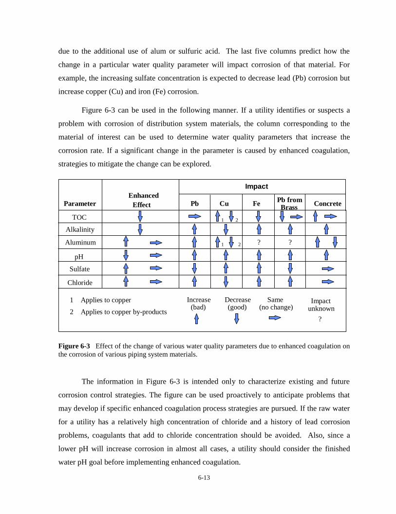
6-13

due to the additional use of alum or sulfuric acid. The last five columns predict how the

change in a particular water quality parameter will impact corrosion of that material. For

example, the increasing sulfate concentration is expected to decrease lead (Pb) corrosion but

increase copper (Cu) and iron (Fe) corrosion.

Figure 6-3 can be used in the following manner. If a utility identifies or suspects a

problem with corrosion of distribution system materials, the column corresponding to the

material of interest can be used to determine water quality parameters that increase the

corrosion rate. If a significant change in the parameter is caused by enhanced coagulation,

strategies to mitigate the change can be explored.

Impact

ParameterEnhanced

Effect Pb Cu Fe Pb fromBrass Concrete

Chloride

Sulfate

Aluminum

pH

Alkalinity

TOC

? ?

1 2

1 Applies to copper

2 Applies to copper by-products

Decrease(good)

Increase(bad)

Same(no change)

Impactunknown

?

1 2

Figure 6-3 Effect of the change of various water quality parameters due to enhanced coagulation onthe corrosion of various piping system materials.

The information in Figure 6-3 is intended only to characterize existing and future

corrosion control strategies. The figure can be used proactively to anticipate problems that

may develop if specific enhanced coagulation process strategies are pursued. If the raw water

for a utility has a relatively high concentration of chloride and a history of lead corrosion

problems, coagulants that add to chloride concentration should be avoided. Also, since a

lower pH will increase corrosion in almost all cases, a utility should consider the finished

water pH goal before implementing enhanced coagulation.

6-14

Figure 6-4 applies to systems implementing enhanced softening. Enhanced softening

does not impact corrosion as much as enhanced coagulation because additional sulfate or

chloride is not usually added. The biggest issue for softening systems is allowing the pH of

the finished water to be higher in the distribution system concurrent with reduced carbonate

buffering capacity. This may lead to widely varying pH values in the distribution system.

Impact

Parameter EnhancedEffect Pb Cu Fe Pb from

Brass Concrete

Chloride

Sulfate

Ca Hardness

pH

Alkalinity

TOC

Decrease(good)

Increase(bad)

Same(no change)

1 2

1 Applies to copper

2 Applies to copper by-products

Figure 6-4 Effect of the change of various water quality parameters due to enhanced softening on thecorrosion of various piping system materials.


Enhanced coagulation and enhanced softening may change the chemistry of the water

entering the distribution system. Before enhanced coagulation or enhanced softening is

implemented, the current corrosion control strategy should be reviewed. This is the first step

in the corrosion control mitigation flowchart shown in Figure 6-5.

The finished water quality parameters discussed in Figures 6-3 and 6-4 can be

examined during a desktop analysis. Based on existing data and literature, a mitigation

strategy can be developed. For example, the finished water pH may be reduced from 7.8 to

7.0 when enhanced coagulation is implemented. The mitigation action may be to provide

6-15

chemical feed facilities to supply base to increase the pH back to 7.8. The characterization

matrices presented earlier can be used to select a mitigation strategy.

After the corrosion control mitigation strategy has been developed, the utility can

ascertain whether the strategy represents a significant change from the current strategy. For

example, if corrosion was minimized by maintaining pH at 7.8 and alkalinity at 60-80 mg/L,

increasing the pH to approximately 7.8 or alkalinity to 60-80 mg/L after enhanced

coagulation would not represent a major change in corrosion control strategy. In this case,

the utility can implement the mitigation actions and continue to monitor the distribution

system for Pb, Cu, and Fe. If the recommended mitigation actions represent a major change

in corrosion control, the utility can conduct pilot-scale (pipe loop) studies to confirm that the

mitigation actions will meet the existing corrosion control goals.

If the utility conducts pilot testing and the results are acceptable, the mitigation

actions can be implemented and the distribution system monitored. If the pilot testing

indicates that the recommended mitigation actions will not provide adequate corrosion

control or the distribution system monitoring identifies a problem, the utility can once again

conduct a corrosion control desktop analysis taking into account the pilot testing data or the

additional distribution monitoring results. This review may lead to another set of

recommended mitigation actions that can be tested.

Cost Implications

Cost impacts may be relatively minor. However, corrosion potential is highly dependent on

site-specific conditions, and some utilities may incur significant costs. Corrosion impacts

may be controlled by changing the pH or by the use of other chemicals. The cost may include

additional chemical facilities or an increase in chemical use. An additional cost also may be

incurred for pilot testing to demonstrate that the corrosion control program is optimized.

Review/complete desktop analysis of corrosioncontrol strategy with EC/ES conditions - Collect finished water quality data - Collect distribution system water quality data

Corrosioncontrol

acceptable?No Action

Yes

No

Recommend mitigation actions

Mitigationactions change corrosion

control strategy?

No

Implement mitigation actions

Monitor Pb, Cu, Fe in distribution system

Is thedistribution

system adverselyimpacted?

No ActionNo

Re-evaluate potential impact ofenhanced coagulation/softening

Yes

Confirmationtest resultsacceptable?

Conduct pilot-scale corrosioncontrol confirmation testing

YesNo

Yes

Figure 6-5. Flowchart for developing a mitigation strategy for corrosioncontrol problems due to enhanced coagulation and enhanced softening

6-17

6.5 PRIMARY DISINFECTION

Enhanced coagulation and softening will have an effect on disinfection by changing

the pH and disinfectant demand. Over the typical plant pH operating range (5.5 - 9.5),

decreasing pH values improves the disinfection characteristics of chlorine and ozone;

decreases the effectiveness of chlorine dioxide; and below a pH of 7.5, tends to lower

chloramine concentrations. The reverse is true for increasing pH values. Disinfection

characteristics outside these pH values are not well understood. The potential effect of

enhanced coagulation and softening on disinfectant effectiveness is summarized in Table 6-1,

and explained in greater detail in this section. Secondary effects and associated mitigation

strategies are discussed in the following sections for chlorine, chloramine, chlorine dioxide,

and ozone.

6.5.1 Chlorine

Lowering pH during enhanced coagulation improves the disinfection characteristic of

chlorine. Increasing pH during enhanced softening decreases the effectiveness of chlorine.

Enhanced coagulation and enhanced softening will reduce the demand for chlorine by

reducing NOM which in turn will improve disinfection efficiency. For enhanced

coagulation, the overall effect of pH reduction and reduced oxidant demand should improve

disinfection efficiency. For enhanced softening, the combined effects of increased pH and

reduced oxidant demand may result in a decrease in disinfection effectiveness. Enhanced

coagulation and softening impacts on chlorine disinfection can be estimated through pilot or

TABLE 6-1 Disinfectant effectiveness under typical operating conditions.

Chlorine Chlorine

Dioxide

Ozone Chlor-

amines

Enhanced

Coagulation

Enhanced

Softening

6-18

jar testing. These tests allow a determination of the pH, chlorine demand, and resultant

chlorine residual before and after enhanced coagulation is implemented. The contact time

(CT) tables in the SWTR Guidance Manual and Part 141, 40 Code of Federal Regulation can

be used to determine if there is a reduction or increase in the level of disinfection.


Mitigation measures will be minor, if at all necessary, for chlorination secondary

impacts because enhanced coagulation usually provides a positive impact. Mitigation

measures for enhanced softening systems should not be significant if the new disinfection

requirements exceed the available chlorination capabilities or available detention time for

chlorine disinfection. The pH can be lowered by recarbonation or acid addition; however,

this should be balanced with the softening and final pH requirements of the process.

Additional chemical facilities to increase the chlorine dose, additional basins to increase the

detention time, process changes, or a change in primary disinfectant can all be used as

mitigation measures, if necessary.

Cost Implications

Cost impacts can be calculated based on a change in the chlorine dose, a change in

detention time, or a change in primary disinfectant. The change in chlorine dose will result in

a change in operating costs. If a change is required in the chlorine feed equipment, there may

be a capital cost increase. If the detention time needs to be increased with new facilities, there

will be a capital cost increase for these facilities. Cost estimates can only be made after the

magnitude of the changes is defined.

6.5.2 Ozone

Reducing the pH and TOC level during enhanced coagulation reduces the ozone

demand and the ozone decay rate. Due to these reductions, a lower ozone dose is required to

achieve an equivalent amount of disinfection. When enhanced softening is practiced prior to

ozonation, the pH of the water should be lowered prior to the ozonation; this may increase

the CO2 dose required during recarbonation. For enhanced coagulation, it is important to

determine the new ozone demand and decay rates. Lower demand and slower decay is

expected. For enhanced softening, it is important to determine the relationship between the

6-19

chemical quantities associated with lowering pH after softening and the additional ozone

dose necessary to achieve the ozonation objectives. Jar and pilot-scale testing procedures

and analysis are presented in Ozone in Water Treatment (AWWARF, 1991).


Enhanced coagulation should reduce ozone demand and decay, resulting in little or no

need for mitigation. There may be a need to more closely monitor the ozone residual leaving

the ozone contactor, because the residual will be longer lived and could carry over to the

filters or other processes. Enhanced softening can cause an increase in CO2 dosage during

the recarbonation step.

Cost Implications

There should be a cost reduction due to reduced ozone application after enhanced

coagulation. Capital cost for new facilities and operating cost for new and existing facilities

may also be reduced. The reduction in dose will result in less generation equipment and a

reduced use of power and gas feed to the ozone generation equipment (e.g., air preparation or

oxygen feed). Changes in cost can be estimated based on the cost estimating procedures

presented in Ozone in Water Treatment (AWWARF, 1991).

6.5.3 Chloramine

Chloramine use and disinfection capabilities will be adversely impacted by enhanced

coagulation. At lower pH, monochloramine is less prevalent, and more di- and tri-

chloramines form which can cause taste and odor problems. At lower pH, there are also

volatility and corrosion problems associated with chloramines.


The pH should be raised prior to chloramination and kept above 7.5 - 8.0 for optimum

chloramine formation. Increasing the pH in the distribution system would have to be

compatible with the corrosion control strategy. An alternate disinfectant also can be

considered. After enhanced coagulation and a corresponding reduction in pH and disinfection

byproduct precursors, it may be possible to use free chlorine for primary disinfection

followed by chloramines for distribution system residual disinfectant. It also may be useful to

6-20

consider changing to an alternative disinfection strategy when considering possible

operational changes.

Cost Implications

Cost impacts may include the need to change pH or change the primary disinfectant.

Capital costs may be incurred if alternative disinfection schemes are used, and operating

costs may be impacted if either an alternative disinfectant is used or the pH is adjusted.

6.5.4 Chlorine Dioxide

Lowering pH may reduce the effectiveness of chlorine dioxide for disinfection,

although the inactivation table in the SWTR Guidance Manual does not reflect this. There

has been some work that suggests that disinfection effectiveness may change with changes in

pH (Finch et al., 1995). There is insufficient data to recommend mitigation of any effects

that enhanced coagulation or softening may have on disinfection effectiveness.

6.6 PARTICLE AND PATHOGEN REMOVAL

Floc Settleability

In some cases, enhanced coagulation may produce a floc that is lighter and more

fragile. This can result in floc carryover from the clarifier to the filters, which could result in

shorter filter runs or premature filter breakthrough and an increase in backwash requirements.

Different Optimal Condition for TOC and particle removal

The lower pH, higher coagulant dose conditions for enhanced coagulation may result

in the restabilization of particles and an increase in the settled water turbidity. Raw waters

that are coagulated under charge neutralization conditions are particularly susceptible to this

problem, because optimal coagulation for TOC and particle removal are different (Carlson et

al., 1996). In one study, Vrijenhoek et al. (1998) observed that under optimized pH

conditions, particle removal may not be adversely affected. Problems also can occur in

solids blanket-type clarifiers. Blanket upset in solids blanket clarifiers may occur with lighter

floc, and control of the system may be harder if the floc is lighter.

6-21

Pre-Filter pH adjustment

Changing the pH prior to filtration may be desirable for additional process objectives

(e.g., Mn removal); however, a change in pH may increase particle breakthrough as well as

increase alum or iron carryover. Adding lime prior to filtration to raise the pH may create

additional problems. It can lead to particle breakthrough, increased solids loading onto the

filters, and reduced filter productivity. For GAC media, it can cause regeneration problems

by increasing the required temperature of regeneration and leaving behind calcium oxide,

which will impact treatment effectiveness when the GAC is reinstalled.

Improved performance is also possible. Less floc carryover and improved filterability

of floc may occur, which improves G. lamblia and C. parvum removal. This can result when

the enhanced coagulation assists in optimizing the coagulation process. Enhanced softening

to a level for magnesium removal may improve particle removal if the plant is designed to

settle magnesium floc. Magnesium floc is lighter and fluffier than calcium carbonate floc and

may carryover in significant amounts if this is not incorporated into the plant design.


The development of a mitigation strategy for particle removal problems due to

enhanced coagulation or softening is presented in Figure 6-6. The first step in the flowchart is

to conduct pilot testing to determine what effect the enhanced coagulation conditions will

have on filter particle removal. Settling performance can be judged with jar testing if the

existing process is used as the control, but filtration must be studied at either pilot- or full-

scale. Ultimately, the full-scale implementation of enhanced coagulation will have to be

monitored and changes to the mitigation strategy may be required due to scale-up issues.

After enhanced coagulation or softening has been tested at pilot-scale, the settled and

filtered water turbidity and particle counts should be compared with the results from the

existing full-scale process. If the enhanced process yields unacceptable settled water results,

the coagulation process should be adjusted to improve particle removal. Polymer addition

(coagulant or floc aid) should be studied to determine if it can improve particle removal.

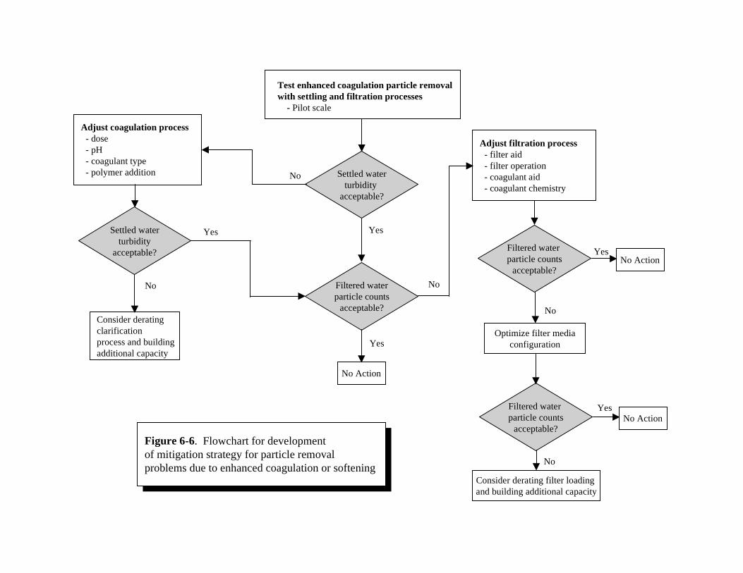
Test enhanced coagulation particle removalwith settling and filtration processes - Pilot scale

Filtered water particle counts

acceptable?

Settled waterturbidity

acceptable?

Adjust filtration process - filter aid - filter operation - coagulant aid - coagulant chemistry

Settled waterturbidity

acceptable?

Filtered waterparticle counts

acceptable?

Filtered water particle counts

acceptable?

Adjust coagulation process - dose - pH - coagulant type - polymer addition

No ActionYes

No ActionYes

Optimize filter mediaconfiguration

No

Consider derating filter loading and building additional capacity

No

No Action

No

Yes

Consider derating clarificationprocess and buildingadditional capacity

No

Yes

Yes

No

Figure 6-6. Flowchart for developmentof mitigation strategy for particle removal problems due to enhanced coagulation or softening

6-23

If these actions do not produce settled water that can meet both TOC and particle

removal goals, utilities may wish to consider derating the clarification process or installing

additional capacity.

Once acceptable settled water turbidity and TOC results are achieved, the filtration

process should be studied. If the filtration process allows unacceptable particle counts in the

filtered water, the filtration process should be adjusted and optimized through the addition of

filter aids. If these remedial actions are not successful, the media configuration should be

studied within the structural constraints of the existing filter boxes.

If the optimized media configuration does not provide acceptable filtered water

particle results, the filters will most likely need to be down-rated. Replacement capacity may

need to be developed. In this case, the cost should be judged relative to the water quality

improvement that will result from enhanced coagulation or softening. If the water quality

improvement is justified, the utility may need to build new filters.

Cost Implications

The cost to mitigate particle removal problems associated with enhanced coagulation

or softening may not be insignificant. As shown in Figure 6-6, the ultimate mitigation

strategy may be the down-rating of existing clarification or filtration facilities. The cost for

mitigation will be considerably less if the coagulation or filtration processes can be improved

by optimizing chemistry, including polymer addition.

Operating costs may rise with an increase in chemical use, increased monitoring due

to less stable operations, and increased operations attention to the processes (e.g., jar testing,

solids monitoring, and increased filter backwashing).

6.7 RESIDUALS HANDLING, TREATMENT, AND DISPOSAL

Implementation of enhanced coagulation or enhanced softening may result in an

increase in the amount of residuals produced during coagulation/softening and filtration. The

increased quantity of solids will result from both the increased coagulant dose and the

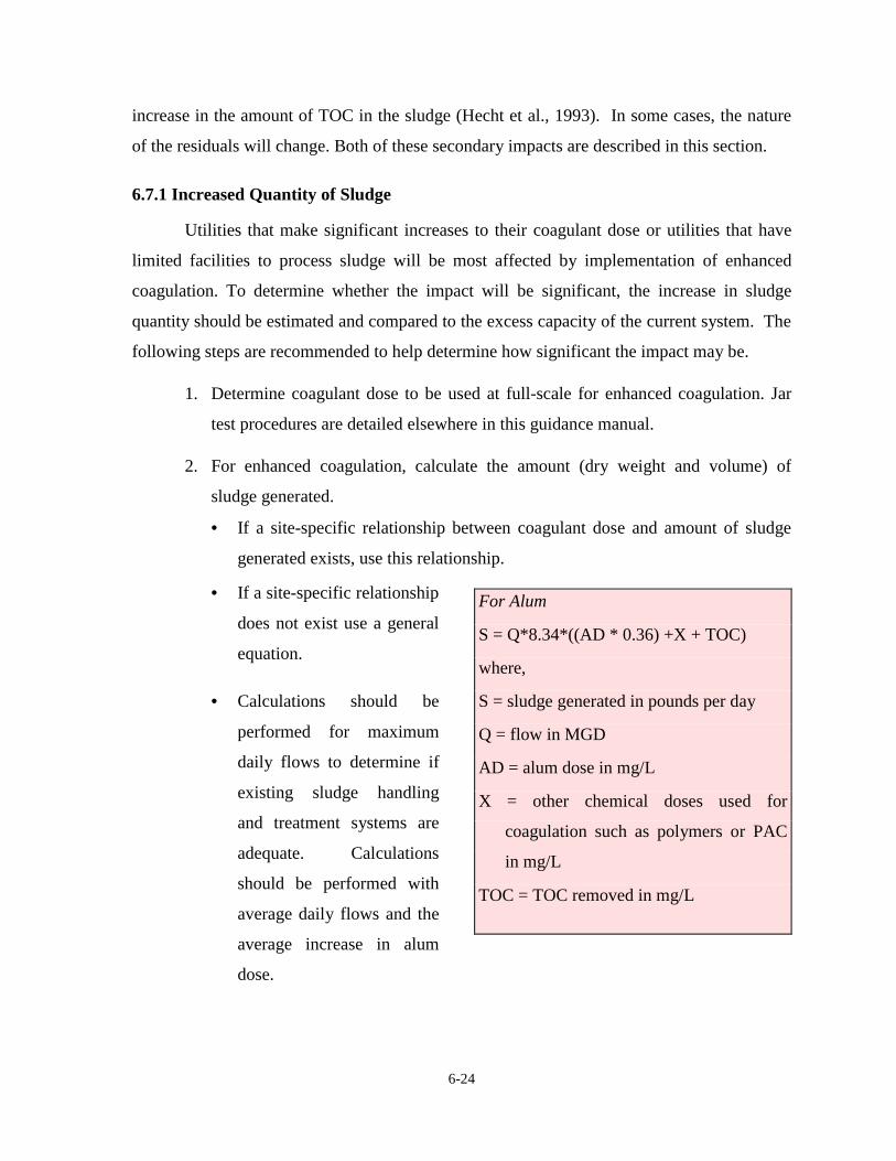
6-24

increase in the amount of TOC in the sludge (Hecht et al., 1993). In some cases, the nature

of the residuals will change. Both of these secondary impacts are described in this section.

6.7.1 Increased Quantity of Sludge

Utilities that make significant increases to their coagulant dose or utilities that have

limited facilities to process sludge will be most affected by implementation of enhanced

coagulation. To determine whether the impact will be significant, the increase in sludge

quantity should be estimated and compared to the excess capacity of the current system. The

following steps are recommended to help determine how significant the impact may be.

1. Determine coagulant dose to be used at full-scale for enhanced coagulation. Jar

test procedures are detailed elsewhere in this guidance manual.

2. For enhanced coagulation, calculate the amount (dry weight and volume) of

sludge generated.

• If a site-specific relationship between coagulant dose and amount of sludge

generated exists, use this relationship.

• If a site-specific relationship

does not exist use a general

equation.

• Calculations should be

performed for maximum

daily flows to determine if

existing sludge handling

and treatment systems are

adequate. Calculations

should be performed with

average daily flows and the

average increase in alum

dose.

For Alum

S = Q*8.34*((AD * 0.36) +X + TOC)

where,

S = sludge generated in pounds per day

Q = flow in MGD

AD = alum dose in mg/L

X = other chemical doses used for

coagulation such as polymers or PAC

in mg/L

TOC = TOC removed in mg/L

6-25

• The volume of residuals can be calculated by assuming a percent solids (based

on the dry-weight calculated

above). It is best to use a site-

specific value for percent

solids, but if one is not

available, 0.5 percent is

typical of sludge from a

clarifier.

3. Compare the calculated volume to each step of the current residuals management

plan or capacity of the existing residuals operation. Look at the following issues:

• basis of system design

• equipment capacity from manufacturers

• permit limits

• sewer capacity

• ultimate disposal capacity

• frequency of cleaning required


Mitigation may involve adjusting the coagulation process to minimize sludge

production. Minimization of sludge production should be balanced with other costs by

optimizing the total cost of treatment, including chemical costs, operating costs, and the cost

of sludge handling. Jar tests can be performed to determine the optimum coagulant type,

coagulation pH, acid dose, and coagulant dose. To mitigate increased residuals produced

during enhanced coagulation, the following variables should be considered when performing

jar tests:

• acid

• acidified coagulant

• polymers

• flocculation pH

• mixing intensity

For Ferric-based coagulants

S = Q*8.34*((FD * 0.5) + X + TOC)

where,

FD = dose of ferric based coagulant

other variables as defined for alum

6-26

Employing acid, acidified coagulant, or polymers may reduce the coagulant dose

necessary to achieve TOC and particle removal. A flowchart for the suggested mitigation

strategy is shown in Figure 6-7. An example is provided below:

Example: Solids Handling Costs

In this example, the EPA water treatment model and plant-scale data were used to

determine the most cost-effective conditions for meeting the requirements for enhanced

coagulation. This example does not include considerations for sludge treatment, but does

demonstrate an approach for comparing coagulation alternatives. In this case, it was

determined that the utility’s two feasible options for enhanced coagulation were alum alone

or a combination of alum and sulfuric acid. Since a new plant was being considered, the

comparison considered capital costs and operating costs for the new plant.

EPA’s water treatment plant model was used to determine the alum dose or the alum

plus acid doses required to reach an optimum coagulation pH of 6.0. The model used the raw

water characteristics for the period September 1996 to August 1997. (Utilities should use

site-specific data to determine coagulant and acid doses.)

The capital cost for a sulfuric acid feed system was estimated to be $282,000, which

does not include any cost savings for a smaller alum system, which would be required if acid

were used.

Operating Costs

There are two areas of significant cost savings associated with the use of sulfuric acid

for coagulation: (1) sulfuric acid is less expensive than alum for pH reduction; and (2) the

amount of sludge produced by using sulfuric acid is considerably less than alum alone.

Chemical Cost Savings

The period of September 1996 to August 1997 was analyzed to determine the

chemical requirements of both options. The following table summarizes the chemical

requirements.

Is sludge treated?No Yes

Enhanced coagulation or softeningimplemented or planned for implementation

Is impact significant?

Yes

No

Consider use of acid to minimizesludge and cost of treatment.

Evaluate impact of enhancedcoagulation treatment on

sludge handling.

Impact likely negligible.Implement and monitor discharge against permit.

Coagulant only Coagulant and acid

Figure 6-7. Impact determinationof increased sludge volume

6-28

Comparison of Average Doses for Enhanced Coagulation

Coagulation Conditions Alum dose (mg/L) Sulfuric Acid dose (mg/L)

Alum alone 90 0

Alum and Sulfuric Acid 45 22

The following costs were based on the annual chemical usage for the period. The unit

price for sulfuric acid used was $125 per ton for 93 percent acid and alum’s unit cost was

$109 per dry ton. The following costs are based on an average daily raw water flow of 30

mgd.

Comparison of Annual Chemical Costs

Coagulation Conditions Cost for Alum Cost for Alum and Acid

Annual costs for alum $448,000 $224,000

Annual costs for acid $0 $137,000

Total Annual Costs $448,000 $361,000

Sludge Costs

The amount of sludge generated by the alum-only scenario is 53.3 mg/L at a dose of

90 mg/L alum (based on EPA’s water treatment plant model). The alum plus acid option,

with alum dosed at 45 mg/L and acid dosed at 22 mg/L, produces 22.8 mg/L of sludge. From

historical data, Waterworks variable costs of residuals handling is $176 per dry ton. Thus, the

alum-only option will produce 6.7 dry tons per day (dpd) versus 2.85 dpd for alum plus acid

under worst case conditions.

On an annual basis, the alum-only solution produces 1,776 dry tons per year (dpy),

versus 1,039 dpy for alum plus acid. The annual cost increase for the alum-only solution is

$130,000. The actual handling costs are $312,576 and $182,864 respectively.

6-29

Total Annual Cost

The total annual costs of concern for this analysis are:

1. Alum only - $761,000

2. Alum + Acid - $544,000

The present value of these differences for an interest rate of 6 percent over twenty

years is:

1. Alum only - $8,729,000

2. Alum + Acid - $6,522,000

Thus, the present value of the cost savings associated with using sulfuric acid is

$2,200,000. The calculations demonstrate that the combination of alum and sulfuric acid is a

more cost-effective solution to reaching optimal coagulation conditions than alum alone, and

that optimal coagulation will produce significant water quality benefits. It is recommended

that a sulfuric acid feed system be designed into the new plant.

To mitigate increased residuals production at enhanced softening facilities consider:

• increasing lime dose, but not exceeding the pH of magnesium hydroxide

precipitation (typically between pH 10.5 to 10.7);

• augmenting with a ferric coagulant;

• avoiding alum because the high pH required for lime softening is outside the

workable pH for alum.

6.7.2 Altered Characteristics of Sludge

When enhanced coagulation is implemented, sludge characteristics may change and

impact its dewaterability (Knocke et al., 1987; Kelkar and Schafran, 1994; McTigue, 1995).

The following are potential changes to sludge characteristics:

• Increased coagulant doses may result in increased percentages of hydroxide

precipitate in the sludge (ferric or alum).

• If acid is used to depress the pH, and the coagulant dose is not decreased, there

may be an increase in the relative TOC content of the sludge.

6-30

• Increased metal concentrations may be experienced. The increased concentrations

may be from natural sources, contaminants in the coagulant, and the coagulant

itself.

• Arsenate not removed by previous coagulation practice may be removed by ferric

coagulants at low pH resulting in arsenate in the sludge.

• When the coagulant dose is increased, there may be a decrease in natural solids to

total solids ratio.

• The time that the sludge is in the clarification basins will decrease if the basins are

cleaned more frequently; therefore, the sludge age will be less.

Typically, these changes are expected to decrease dewaterability; however, in some

cases dewaterability may be improved. If significant changes in coagulant dose or pH are

required, pilot testing of residuals dewatering is recommended. If no residuals treatment is

provided, then the impact is limited to changes related to the permit for ultimate disposal.

Monitoring may be appropriate to determine the nature of the discharge after enhanced

coagulation is implemented; monitoring issues are discussed in greater detail later in this

section.

One issue that is specific to enhanced softening is the potential formation of

magnesium hydroxide [Mg(OH)2 ] precipitate. Softening plants that are designed for CaCO3

removal may form Mg(OH)2 at the increased pH levels that result from increased lime doses

required to meet enhanced softening requirements. Mg(OH)2 production can increase

quickly as pH levels of 10.5 to 10.7 are approached. The exact pH varies with each water

type, and the amount of Mg(OH)2 produced depends on how much Mg is present in the water

before treatment. Since Mg(OH)2 is more difficult to dewater than CaCO3, enhanced

softening may significantly increase solids handling requirements. In addition, the amount of

additional lime required to change the pH can result in a significant increase in sludge

volume regardless of whether magnesium is precipitated.

6-31


The mitigation steps for enhanced coagulation are summarized in the flowchart

presented in Figure 6-8. The mitigation steps are divided into two categories, based on

whether the residuals are treated by thickening or dewatering. If no residuals treatment is

provided, then the impacts may be negligible. The nature of the sludge should be monitored

for items covered by the discharge permit to determine whether enhanced coagulation

conditions will jeopardize permit conditions. If testing indicates that permit conditions cannot

be met when enhanced coagulation is implemented, utilities should consider altering

coagulation conditions as previously discussed (e.g., using acid to depress pH), or consider

providing some treatment for the residuals. Treatment could be as simple as providing

additional settling time.

If residuals treatment is provided, then pilot-scale testing of residuals treatment under

the enhanced coagulation conditions can be considered. Pilot-scale testing would focus on

determining whether the existing residuals treatment facilities need to be adjusted to provide

desired treatment. During pilot testing, the water quality of any permitted disposal streams

should be monitored to verify that permit conditions can be met. If existing facilities are

found to be inadequate, consider the following options:

• Change the chemical conditioning of the sludge; for example, try a different

polymer or bentonite addition.

• Use alternative technologies to treat the sludge; for example, dewatering with a

centrifuge rather than a belt press.

• Alter the water treatment mechanisms that may affect sludge treatment; for

example, implement air scour during backwash to minimize the production of

waste washwater.

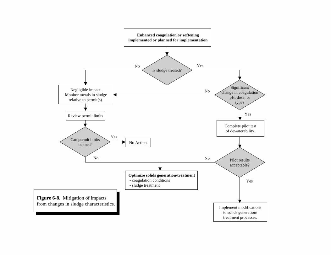
Is sludge treated?No Yes

Enhanced coagulation or softeningimplemented or planned for implementation

Significantchange in coagulation

pH, dose, ortype?

Yes

No

Complete pilot testof dewaterability.

Implement modificationsto solids generation/treatment processes.

Negligible impact.Monitor metals in sludge

relative to permit(s).

Figure 6-8. Mitigation of impactsfrom changes in sludge characteristics.

Pilot resultsacceptable?

Yes

Review permit limits

Can permit limitsbe met?

Optimize solids generation/treatment - coagulation conditions - sludge treatment

No ActionYes

No No

6-33

6.8 OPERATION AND MAINTENANCE

Changing from an operational strategy designed to remove turbidity to one that

includes TOC removal will require some changes in the operation and maintenance of the

coagulation system. The following are some changes that may result due to the

implementation of enhanced coagulation and enhanced softening:

• A change in type or dose of coagulant and/or polymer aid may be required. Also,

the optimal range of coagulant aid can be reduced. Increasing the lime dose in

softening plants can result in the production of more Mg(OH)2, which does not

settle as readily as CaCO3.

• A change in coagulation conditions may require greater vigilance by operators to

control the carryover of floc from the settling basins to the filters. If floc

carryover to the filters occurs, more frequent backwashing of the filters will be

necessary requiring more water, electricity and labor. Also, increased floc

carryover may cause “mudballs” to form in the filter media if the backwash is not

sufficient.

• Increased coagulant and lime doses may increase the sludge removal frequency.

• Corrosion in metals or concrete may occur at low pH values. The potential for and

extent of this impact is uncertain.


The following points could be considered in developing mitigation strategies for

resolving operation and maintenance problems:

• Education of the operations staff to communicate the regulatory needs, operating

philosophy, and the benefit of the enhanced coagulation/enhanced softening may

be helpful.

6-34

• A streaming current monitoring system can be augmented with a pH control

monitoring system. TOC or UV-254 (in oxidant-free situations) can be monitored

more frequently or in-line to provide a better handle on the operation of the

coagulation process.

• Frequent jar testing should be carried out to determine appropriate coagulation

conditions (simultaneous removal of TOC and particles).

• Operators should be more vigilant about removal of precipitated solids from

sedimentation basins and sludge-blanket clarifier and backwashing of filters.

• Proper use of polymers is expected to improve settleability and filterability of

flocs, however, the operators should be cautious about overdosing of polymers

which can adversely effect the filter media.

• Installation of plate or tube settlers may improve removal of solids in clarifiers.

• Periodic application of paints or acid resistant coating on the submerged

mechanical parts and concrete surfaces is expected to reduce in-plant corrosion.

6.9 RECYCLE STREAMS

The effect of enhanced coagulation or enhanced softening on the quality of recycle

streams can be substantial if the coagulant dose is increased significantly. Conversely, if the

coagulation conditions are not significantly changed, the recycle stream may not be

impacted. The nature of the effect will depend on whether or not the recycle stream is treated.

If recycle treatment is provided, an increase in the volume of the recycle may overwhelm the

existing recycle treatment system, especially if this system is near capacity.

In the context of this document, untreated recycle refers to recycle streams that are

not treated and are added directly into the process flow stream. In some cases, increased

recycle flow may upset the treatment process. Typically, process flow may not be impacted

when the recycle comprises less than five percent of the process flow.

6-35

With softening plants, the potential to form a Mg(OH)2 precipitate presents a special

issue related to recycling during enhanced softening. In plants treating water with more than

approximately 40 mg/L of Mg, there is potential to form a Mg(OH)2 precipitate. Once this

precipitate is in the recycle system, it would be difficult to remove from the plant because it

settles poorly compared to calcium carbonate.


The mitigation efforts are different for plants that treat recycle and those that do not

provide treatment. For plants that do not provide treatment (i.e., those that recycle directly)

the operational impacts can be mitigated by:

• adding a new equalization basin or increasing the capacity of the existing

equalization basin;

• treating the recycle, for example, installing solids separation;

• eliminating all recycling; and

• send flow to a sanitary sewer.

For those plants that do provide treatment of the recycle system, the mitigation efforts

are somewhat site-specific, depending on the nature of the treatment provided. Some of the

more common mitigation steps include the following:

• Optimize existing equalization provided by existing recycle treatment facilities

(e.g., thickener).

• Expand the recycle treatment system.

• Consider alternate disposal options; for example, send the waste or a portion of

the waste to the sewer.

• Consider chemical treatment, such as polymer, to increase the capacity of the

treatment system.

• Consider upgrades to thickener, such as plates or tubes, to augment settling.

• Avoid increasing pH beyond the threshold where significant formation of

Mg(OH)2 occurs (approximately 10.5).

Chapter 7

FULL-SCALE IMPLEMENTATION OF TREATABILITY STUDIES

Table of Contents

Page

7.0 FULL-SCALE IMPLEMENTATION OF TREATABILITY STUDIES7.1 Introduction . . . . . . . . . . . . . . . . . . . . . . . . . . . . . . . . . . . . . . . . . . . . . . . . 7-17.2 Scale-Up Issues for Treatability Test Results. . . . . . . . . . . . . . . . . . . . . . . 7-2

7.2.1 Coagulation and Flocculation. . . . . . . . . . . . . . . . . . . . . . . . . . . . 7-27.2.2 Sedimentation. . . . . . . . . . . . . . . . . . . . . . . . . . . . . . . . . . . . . . . . 7-3

7.3 Unit Process Issues . . . . . . . . . . . . . . . . . . . . . . . . . . . . . . . . . . . . . . . . . . . 7-47.3.1 Chemical Addition. . . . . . . . . . . . . . . . . . . . . . . . . . . . . . . . . . . . 7-47.3.2 Rapid Mixing and Flocculation. . . . . . . . . . . . . . . . . . . . . . . . . . 7-67.3.3 Sedimentation. . . . . . . . . . . . . . . . . . . . . . . . . . . . . . . . . . . . . . . . 7-77.3.4 Filtration . . . . . . . . . . . . . . . . . . . . . . . . . . . . . . . . . . . . . . . . . . . . 7-97.3.5 Sludge Handling. . . . . . . . . . . . . . . . . . . . . . . . . . . . . . . . . . . . . 7-10

7.4 Other Full-Scale Implementation Issues . . . . . . . . . . . . . . . . . . . . . . . . . . 7-10

List of Tables

7-1 National Sanitation Foundation Product Limits on Chemical Additives. . . . . . 7-6

7-1

7.0 FULL-SCALE IMPLEMENTATIONOF TREATABILITY STUDIES

7.1 INTRODUCTION

Previous chapters have described the contents of the DBPR, methods for removal of

NOM, the definitions of enhanced coagulation and enhanced precipitative softening, and

testing and laboratory protocols. This chapter provides guidance on how to use these

methods and protocols to enhance full-scale performance. This chapter provides guidance

on the incorporation of treatability studies (i.e., jar or pilot-scale testing) into full-scale

processes, and offers suggestions for unit process changes which may help meet the TOC

removal requirements. The success and ease of full-scale implementation of enhanced

coagulation and enhanced precipitative softening will depend on a utility’s planning and

development of implementation strategies, as well as the incorporation of these strategies.

Results of treatability testing should be evaluated in the light of the secondary effects

of enhanced coagulation (discussed in Chapter 6) in order to adequately plan for process

modifications in the full-scale facilities. Based upon the extent of process modifications

required, some utilities may need to begin the planning process significantly ahead of the

effective date of the rule so that adequate capital improvement budgets are available to make

the necessary process changes. Planning for full-scale process modifications for compliance

with enhanced coagulation requirements may include modifications to: (1) chemical feed

systems (e.g., metal coagulant, polymeric coagulant, pH depressing chemicals, and pH

raising chemicals); (2) operation of unit processes (e.g., flocculation, sedimentation, and

filtration); and (3) operation of sludge handling systems. In the planning efforts, the issues

related to scaling up of bench- or pilot-scale process studies also need to be considered. This

chapter presents a discussion of potential modifications to various plant operations resulting

from enhanced coagulation, and offers suggestions for the development of full-scale

implementation strategies.

7-2

7.2 SCALE-UP ISSUES FOR TREATABILITY TEST RESULTS

7.2.1 Coagulation and Flocculation

Coagulation/flocculation is a physical/chemical process that can usually be adequately

simulated through jar testing, and the effectiveness of a coagulant can often be determined

using jar tests (Amirtharajah and O’Melia, 1990). Coagulation/flocculation involves

chemical reactions and interparticle contacts that occur very rapidly, which allows rapid

mixing to be reasonably simulated at the bench (batch) scale. Short-circuiting does not occur

during jar testing. Thus, results from jar-test trials of flocculation may be superior to those

in plants where short-circuiting in the mixing and flocculating processes occurs. However,

flocculation at full-scale facilities typically uses external energy input through a variety of

mixing mechanisms (e.g., turbine, horizontal paddle) as well as a designated detention time.

Therefore, as long as the energy input and detention times are simulated accurately during

jar testing, full-scale performance of flocculation can be relatively well-simulated.

The carbon dioxide exchange between the water in the jars during bench-scale testing

and the ambient atmosphere could potentially be different compared to full-scale basins and

pipe lines (for static mixers). In a full-scale facility the amount of surface area exposed to

the atmosphere for a given volume of water may be significantly smaller than the exposed

area in a 1- or 2-liter jar. As a result, carbon dioxide can more readily transfer between the

water and the air during jar tests, resulting in more dramatic pH changes compared to the

full-scale process. Since the pH of coagulation is closely associated with the NOM removal

ability of metal coagulants, jar testing results may not always be reproducible at full-scale.

The jar test results may overestimate particle removal and underestimate TOC removal. If

the jar test pH values are also used to determine the amount of base necessary to raise the pH

before distribution, this amount may also be underestimated compared to the amount

necessary at full-scale. Covers on the jars will help reduce the exchange of carbon dioxide

during jar tests (see Section 3.2.2.1).

7-3

7.2.2 Sedimentation

For many waters, there is a wide range of conditions in which floc adequately entraps

organic matter and turbidity, but finding the optimum condition for rapid settling of the floc

can be a difficult task (Hudson, 1981). Efficient settling is extremely important because it

minimizes the floc loading onto the filters. Shorter filter runs and a reduction in treatment

capacity can result from poor sedimentation. Settling velocity distribution curves are used

to analyze floc settling characteristics during jar testing by collecting samples at a given

depth over discrete time intervals. The settling velocities can be compared to full-scale

surface loading (overflow) rates on sedimentation basins. Therefore, when floc settling

characteristics are compared for different jar test conditions, the settling velocity distribution

curves should be translated to the surface loading rate of the sedimentation basin.

Care should be taken in projecting jar test settling data to full-scale plant operation due

to the longer detention time at full-scale compared to jar tests. For a given settling velocity,

the detention time in the jar test procedure is about 1/60 of that in a conventional plant.

Residence time in full-scale plants is commonly on the order of several hours, although

shorter detention times may be found in plants using tube or tray settlers with short settling

times. Experience has shown that the settling obtained in plants with well-designed mixing

and flocculation facilities is usually superior to jar test results. This is likely caused by

continued flocculation in the settling basin due to differential settling velocities for different

size particles. Another factor is the continued rotation of the water in the jar testing

equipment after the flocculating paddles are stopped. The use of stators or square jars helps

reduce this rotation (see Section 3.2.2.1). Apparently, the effect of continued rotation after

the paddles have stopped approximates the typical effect of turbulence at the settling basin

inlet. For these reasons, jar test results may underestimate the settling performance that may

be achieved at full-scale.

Given these considerations, the recommended period for settling during jar testing is

between 30 and 60 minutes. This duration has been shown to produce a clear supernatant

for floc that will settle adequately at full-scale.

7-4

7.3 UNIT PROCESS ISSUES

7.3.1 Chemical Addition

Implementation of enhanced coagulation may require substantial alteration of

coagulant doses at some treatment plants. Some plants may also need to add new chemicals,

such as acid or caustic, to improve coagulation. Other plants may require only minor

adjustments to their chemical additives to comply with enhanced coagulation requirements.

For plants that may require significant changes, adequate planning should be done to assure

compliance with treatment requirements.

Based on the results of treatability testing, utilities should estimate changes in current

chemical doses as well as the potential need for additional chemicals such as: (1) acid to

depress pH for enhanced coagulation (in such instances, increased dosages of lime and

caustic also will be required to increase pH prior to distribution); or (2) increased dosages

of CO2 if lime dosages are increased in lime softening systems. The utility should develop

a plan for compliance based upon the treatability testing, the operator’s experience, and the

condition and capacity of the existing facilities (chemical feed, chemical storage, and sludge

handling). Some important factors to consider in assessing the potential need for facility

modifications include:

• Adequacy of the storage (bulk-storage and day tanks) and feed facility (meteringpumps, electronic controls for metering pumps, etc.) for metal coagulants, polymericcoagulants and filtration aids. Many States require utilities to have at least a 30-day,on-site, bulk-storage capacity under average demand conditions. An increase inchemical dosages, therefore, may require the utility to design and construct additionalstorage and feed facilities.

• The need for an additional chemical to depress pH in enhanced coagulation toachieve more effective TOC removal at lower pH values. Sulfuric acid is the mostcommonly used chemical for lowering pH during coagulation. Softening plants usecarbon dioxide for pH depression during recarbonation, however, carbon dioxide isalso used in some plants for lowering coagulation pH. In selecting an appropriatechemical to modify pH, relative costs, handling considerations, and operator safetyneed to be considered. It should be noted that the addition of carbon dioxide is oftenmore expensive than sulfuric acid, but does not require handling of a listed hazardouschemical.

7-5

• If the pH of coagulation is too low (or in the case of lime softening, too high) fordistribution, the pH needs to be increased (or decreased for lime softening). In plantspracticing coagulation, lime is often added in the coagulation process to controlfinished water pH. Unfortunately, this practice does not allow the utility to achievethe full benefit of a lower coagulation pH. Consequently, increasing pH afterfiltration could be a better alternative with respect to TOC removal and chlorinedisinfection. Sodium hydroxide is often recommended for raising pH after filtration.If a plant is not already equipped with a caustic feed system, proper planning anddesign need to be considered for this chemical if enhanced coagulation pH is lowerthan the acceptable distribution system pH.

In addition to the above considerations, the following general factors need to be

considered for any new design or modification of chemical feed systems:

• Chemicals should be added to ensure proper dispersion across the entire flow. Inmost cases coagulant should be applied through perforated troughs or perforated pipediffuser systems in order to distribute it across the stream of water. A confined,narrow path at the chemical injection point is recommended to improve chemicaldistribution. The diffuser should be located at a point immediately upstream of thezone of highest available turbulence. If a mixing device such as a turbine or pumpis used, the coagulant should be applied as close to the impeller as possible. Thismethod has been found to be more effective than a channel diffuser, which lackssupplemental mechanical agitation.

• For effective flash mixing, dilution of the coagulant solution to a concentration of 2.5to 5 percent is recommended (James M. Montgomery, 1985). Larger volumes aremore easily and quickly dispersed into a large body of raw water than smallervolumes. At concentrations of less than 1 percent, however, alum may dissociate andalum floc or scale [Al(OH)3] may form, clogging feed lines or orifices. For thisreason, alum or ferric salts generally should not be diluted below 2.5 percent priorto addition to raw water.

• The proper sequence of chemical injection is important when more than one chemicalis added to the raw water. As discussed previously, it may be necessary to add acoagulant aid to assist in forming a well-settling floc. The proper chemical sequenceis best determined by testing the raw water and chemical combination during jartesting. For example, anionic polymers are usually most efficient when they are fedto raw water after alum addition, once pin-point flocs have been formed. If a cationicpolymer is used as a coagulant aid, the time of mixing becomes less importantbecause polymers react directly with NOM and particulate matter.

• Some lime softening plants add ferric sulfate or ferric chloride to the lime floc toimprove settling and TOC removal, in lieu of a polymer. The extent to which this issuccessful depends on the nature of the source water and the lime softening dosage.

7-6

Table 7-1 lists some product limits for the addition of chemicals commonly used in

coagulation and flocculation systems. These limits are based on National Sanitation

Foundation (NSF) standards (ANSI/NSF Standard 60), and are product-specific, depending,

in part, on the impurities present in the chemical products.

TABLE 7-1National Science Foundation

Product Limits on Chemical Additives

Chemical Additive Maximum Use a

Alum 150 mg/L

Ferric Sulfate 200 - 600 mg/L

Ferric Chloride 141 - 250 mg/L

Sulfuric Acid 50 mg/L

Polyaluminum chloride (PACl) 100 - 454 mg/L

Note: a - The limits shown here are for general guidance only. Each product (i.e., brand or trademark)has limits specific to that product, depending on the chemical nature of the additive andimpurities present. The numbers in this column represent a range of the limits recommended for several brands of additives.

7.3.2 Rapid Mixing and Flocculation

Changes in chemical feed systems as a result of the implementation of enhanced

coagulation are not expected to alter the rapid mixing and flocculation processes in a water

treatment plant. Potentially greater quantities of floc could form if significantly larger doses

of coagulant chemicals are used for compliance with the enhanced coagulation requirements.

For this reason, care should be taken to ensure adequate agitation during the flocculation

stage so that floc does not settle out in this process. Settling of floc in the flocculation stage

may result in loss of effective volumes since flocculation basins are often not equipped with

any sludge removal mechanisms.

Significantly altering chemical addition schemes for compliance with enhanced

coagulation may require some changes in the mixing conditions to properly develop

settleable and filterable floc. Utilities are encouraged to conduct bench- or pilot-scale

7-7

evaluations to determine the optimum mixing conditions under the altered chemical addition

schemes for enhanced coagulation. The following general design issues need to be

considered during the development of enhanced coagulation implementation strategies:

• The purpose of rapid mixing is to obtain instantaneous, uniform dispersion of thecoagulant through the raw water, since the most efficient use of the coagulant isachieved with instantaneous dispersion. Rapid chemical dispersion is generallyobtained by some type of diffuser in combination with hydraulic turbulence.Conventional rapid-mixing chambers, which have a 10 to 30 second retention timeand use 0.25 to 1.0 hp/mgd of mechanical mixing, have velocity gradients in the rangeof 300 to 1000 sec-1.

• The aggregation of optimum-size flocs (0.1 to 2.0 mm effective size) requires gentlemixing in the energy gradient range of 20 to 70 s-1 for a period of approximately 20minutes (Hudson, 1981). For settling, a larger visible floc is normally required, andlower energy levels are applied. Smaller, more dense floc is formed at the high endof the energy range.

• The gentle mixing process of flocculation is designed to maximize contact ofdestabilized particles and build settleable or filterable floc particles. Shear forcesshould be maintained constant within the mixing process. Flocculator mechanismstend to be slow and tend to cover the maximum possible cross-sectional area of theflocculation basins.

• Dividing the process into two or more defined stages or compartments will helpprevent short-circuiting and permit defined zones of reduced energy input. To ensurethat short-circuiting does not occur, baffles are typically placed between each stage offlocculation. For mechanical (non-hydraulic) flocculation basins, the baffles aredesigned to provide an orifice ratio of approximately 3 to 6 percent or a velocity of 0.3m/s (0.9 fps) under maximum flow conditions.

7.3.3 Sedimentation

Higher coagulant and lime dosages result in greater quantities of settleable particles

that will be separated during the sedimentation process. For this reason, the sludge removal

mechanisms may need to be operated on a more frequent basis. This may, in turn, increase

the short-circuiting induced by the movement of the sludge removal device. As discussed

in Section 7.3.2, utilities need to consider bench- and pilot-scale testing to ensure that the

particles produced during enhanced coagulation can settle properly in the sedimentation

process. In developing strategies for implementing enhanced coagulation or enhanced

7-8

precipitative softening, utilities need to consider the settling characteristics of the floc.

Although it is unlikely that the utilities will need to substantially modify the design or

operation of their sedimentation basins, some utilities may need to consider minor

modifications to improve solids removal by settling. The following factors should be

considered in deciding on sedimentation process improvement:

• Control measures to aid sedimentation and to minimize or eliminate short-circuitingcaused by density currents include: (1) use of a surface weir or launder takeoff overa large part of the settling basin, (2) improved inlet arrangements, and (3) schemes toprovide increased basin drag and friction (Hudson, 1981).

• Various baffling methods could be considered for improving the turbulence at theentrance to the sedimentation basins. One of the most successful methods is theperforated baffle (Hudson, 1981). Proper design of perforated baffles requires fourconditions to be met:

1. The head loss through the ports should be about four times higher than the kineticenergy of approaching velocities to equalize both horizontal and vertical flowdistribution.

2. To avoid break-up of floc, the velocity gradient through inlet conduits and portsshould be kept close to that in the last compartment of the flocculators.

3. The maximum feasible number of ports should be provided to minimize the lengthof the turbulent entry zone produced by the diffusion of the submerged jets fromthe ports in the perforated-baffle inlet.

4. The port configuration should assure that the discharge jets will direct the flowtoward the basin outlet.

• Discharge weirs can be extended into the basin up to half of the basin length. Thisreduces the localized upflow velocity and discourages re-entrainment of settled floc.Perforated launders can also be used to minimize passage of floatable material (thatsometimes can accumulate as the result of polymer addition or with metal coagulants)and further reduce local, upflow velocities.

• The performance of existing basins may be substantially improved by adding tube orplate settlers. These units use inclined tubes or plates to increase the overall removalsurface area and decrease the distance a particle must settle before it is captured. Forefficient self-cleaning, tube or plate settlers are typically installed at a 45o to 60o angleabove horizontal. The open distance between the plates (or the diameter of the tube)is typically about 2 inches (5 cm), although there are a variety of configurationsmarketed by several manufacturers (Hudson, 1981).

7-9

7.3.4 Filtration

If the implementation of a modified chemical treatment strategy affects the settled water

quality in a treatment plant, the performance of the filters can also be affected. This may

manifest itself by early particle or turbidity breakthrough in the filters, which may ultimately

result in shorter filter runs. Utilities may need to evaluate alternatives to improve filter

performance or to plan for shorter filter runs. One impact of shorter filter runs is an increase

in the amount of filter backwash water. If a utility recycles filter backwash water, an increase

in the volume of filter backwash water may stress the unit processes (such as equalization

basin, backwash water treatment processes, etc.) that treat the recycle stream. Adequate

planning for implementation of enhanced coagulation and enhanced precipitative softening

should include an assessment of the volume of filter backwash and its subsequent

downstream impacts. Utilities which expect to have large increases in chemical doses should

consider pilot-scale evaluations to estimate the quality of settled water and the performance

of filters. The following chemical improvements to the operation of filters may be

considered as a part of the planning for enhanced coagulation and enhanced precipitative

softening:

• Careful selection of a coagulant aid and filter aid is critical to improve settling in thesedimentation basin and minimize particle breakthrough in the filters. The use of afilter-aid polymer can result in improved particle capture, better filtrate quality, longerfilter runs, and higher headloss prior to turbidity breakthrough. Filter aids are oftenfed in dilute liquid form to allow dispersion without mechanical agitation just priorto filtration. Filter-aid polymer dosages to gravity filters are usually low (0.03 to 0.05mg/L). Doses required for pressure filters may be higher if a higher operatingheadloss is employed. Because the viscosity of water increases with decreasingtemperature, breakthrough as a result of floc shearing is more likely at lower watertemperatures. Consequently, increased polymer doses may be required in coldweather. A longer contact time prior to filtration may also be necessary in coldweather.

• The type of polymer to be added also needs careful consideration. Polymers used asfilter aids are generally categorized into cationic, anionic, and nonionic groups. Themost appropriate choice will be site-specific, and typically will be verified throughtrial and error. Many plants, however, have had greater success with nonionic andanionic polymer filter aids. Cationic polymers have shown superior performance ascoagulant aids rather than as filter aids. The molecular weight of the polymer mustalso be considered. Many plants have had greater success with higher molecular

7-10

weight compounds, but individual applications will be very dependent on site-specificconditions.

• Two methods are typically used to determine the optimum dose for filter aids. Todetermine the optimum dose for particle destabilization, jar tests with extendedflocculation periods may be used, especially for the destabilization of low-turbiditywaters. Another obvious method to determine optimum dose consists simply ofsystematically varying the dosage over a filter run and monitoring the effluent waterquality and filter performance. Both these techniques have been found to producesimilar results (AWWARF, 1989).

7.3.5 Sludge Handling

Increasing coagulant and lime dosages for enhanced coagulation and enhanced

precipitative softening, respectively, will have an impact on sludge production. Depending

upon the extent of the dosage increases and the nature of the sludge handling system, the

impacts of increased sludge production can be significant. If dosages are modified

significantly, it is critical that systems evaluate the capacity of their sludge handling systems

and consider whether upgrades and expansions are required. In some instances, the method

of sludge handling may change. For example, if a system has been discharging to the sewer,

but the capacity of the piping and/or the allowable discharge to the wastewater system is

limited, it may be necessary to provide some sludge handling on-site. These types of changes

are particularly significant and represent costs which are not directly related to the chemical

feed facilities. These impacts are discussed in detail in Section 6.7.

7.4 OTHER FULL-SCALE IMPLEMENTATION ISSUES

Some secondary effects can be anticipated with the implementation of enhanced

coagulation, such as increased corrosion (due to pH reductions), increased sludge production,

decreased sludge dewaterability and settleability, and increases in inorganic contaminants

(i.e., Al, Mn, Fe). Other concerns also arise upon implementation of enhanced coagulation,

such as the potential degradation of a plant’s ability to produce a safe and aesthetically

acceptable water; customer perception of the new water quality; and the long-term

distribution system integrity. Treatment techniques and changes in operation may be

7-11

required to resolve these problems. The underlying issue revolving around these concerns

is ultimately an increase in operational costs. Utilities need to address these concerns before

implementing enhanced coagulation to avoid future problems. Chapter 6 provides an outline

of the important secondary effects of enhanced coagulation, and includes some guidance to

resolve these foreseeable problems.

Appendix A

DBP PRECURSOR REMOVAL PROCESSES

Table of Contents

Page

A.0 DBP PRECURSOR REMOVAL PROCESSES

A.1 Introduction . . . . . . . . . . . . . . . . . . . . . . . . . . . . . . . . . . . . . . . . . . . . . A-1A.2 Surrogate Parameters for NOM (DBP Precursor) Removal . . . . . . . . . A-2

A.2.1 Introduction . . . . . . . . . . . . . . . . . . . . . . . . . . . . . . . . . . . . . . A-2A.2.2 Total and Dissolved Organic Carbon . . . . . . . . . . . . . . . . . . . . A-3A.2.3 Ultraviolet Light Absorbance at 254 nm . . . . . . . . . . . . . . . . . A-4A.2.4 Specific Ultraviolet Absorption (SUVA) . . . . . . . . . . . . . . . . . A-4A.2.5 Trihalomethane Formation Potential . . . . . . . . . . . . . . . . . . . . A-5

A.2.5.1 THMFP Test . . . . . . . . . . . . . . . . . . . . . . . . . . . . . . A-5A.2.5.2 Simulated Distribution System Test . . . . . . . . . . . . . A-6A.2.5.3 Uniform Formation Conditions Test . . . . . . . . . . . . . A-6

A.2.6 Summary . . . . . . . . . . . . . . . . . . . . . . . . . . . . . . . . . . . . . . . . A-7A.3 Characteristics of Natural Organic Matter . . . . . . . . . . . . . . . . . . . . . . A-7

A.3.1 Humic/Non-Humic Fractionation . . . . . . . . . . . . . . . . . . . . . . A-7A.3.2 Molecular Weight Fractionation . . . . . . . . . . . . . . . . . . . . . . . A-8

A.4 Treatment Technologies for DBP Precursor Removal . . . . . . . . . . . . . A-9A.4.1 Chemical Coagulation . . . . . . . . . . . . . . . . . . . . . . . . . . . . . . . A-9A.4.2 Precipitative Softening . . . . . . . . . . . . . . . . . . . . . . . . . . . . . A-12A.4.3 Preoxidation . . . . . . . . . . . . . . . . . . . . . . . . . . . . . . . . . . . . . A-14

A.4.3.1 Chlorine . . . . . . . . . . . . . . . . . . . . . . . . . . . . . . . . . A-14A.4.3.2 Chloramines . . . . . . . . . . . . . . . . . . . . . . . . . . . . . . A-17A.4.3.3 Ozone . . . . . . . . . . . . . . . . . . . . . . . . . . . . . . . . . . . A-18A.4.3.4 Chlorine Dioxide . . . . . . . . . . . . . . . . . . . . . . . . . . A-19A.4.3.5 Potassium Permanganate . . . . . . . . . . . . . . . . . . . . A-20A.4.3.6 Advanced Oxidation Processes . . . . . . . . . . . . . . . . A-21

A.4.4 Separation Processes . . . . . . . . . . . . . . . . . . . . . . . . . . . . . . . A-21A.4.4.1 Sedimentation . . . . . . . . . . . . . . . . . . . . . . . . . . . . . A-21A.4.4.2 Dissolved Air Flotation . . . . . . . . . . . . . . . . . . . . . . A-22A.4.4.3 Filtration . . . . . . . . . . . . . . . . . . . . . . . . . . . . . . . . . A-22

A.5 Other Precursor Removal Technologies . . . . . . . . . . . . . . . . . . . . . . . A-23A.6 Summary . . . . . . . . . . . . . . . . . . . . . . . . . . . . . . . . . . . . . . . . . . . . . . A-23

List of Tables

A-1 Impact of Moving Point of Chlorination on DBP Formation . . . . . . . . . . . . . . . . A-17A-2 Use of Chlorine Dioxide for THMFP and TOXFP Removal . . . . . . . . . . . . . . . . A-19

List of Figures

A-1 Process Flow Schematic for a Conventional Water Treatment Plant . . . . . . . . . . A-10A-2 Process Flow Schematic for a Lime Softening Water Treatment Plant . . . . . . . . A-13A-3 Typical Ozone Oxidation Process . . . . . . . . . . . . . . . . . . . . . . . . . . . . . . . . . . . . A-15

A-1

APPENDIX ADBP PRECURSOR REMOVAL PROCESSES

A.1 INTRODUCTION

Natural organic matter (NOM) is ubiquitous in surface and ground water sources.

NOM consists of humic substances, amino acids, sugars, aliphatic acids, aromatic acids and

a large number of other organic molecules. Although interest in NOM research and removal

has primarily revolved around the reactions between NOM and chemical disinfectants, a water

system should consider enhancing existing treatment practices for removal of NOM for

several other reasons. NOM has been shown to bind with harmful metals and synthetic

organic chemicals (SOCs), thereby allowing these contaminants to proceed through treatment

processes not designed to remove NOM. In addition, NOM creates a disinfectant demand

and forces utilities to use higher disinfectant dosages to maintain an adequate residual in water

distribution systems. Some NOM components may also provide food for microorganisms in

these distribution systems. NOM also competes with other organic compounds which are

amenable to adsorption by powdered activated carbon (PAC) or granulated activated carbon

(GAC).

This appendix focuses on treatment technologies that have been evaluated for their

ability to remove NOM, and how coagulation and precipitative softening compare to other

NOM (DBP precursor) removal processes. However, the characteristics and measures of

NOM have important implications with regards to the performance and evaluation of these

processes. Sections A.2 and A.3 summarize these characteristics and measures; Section A.4

describes treatment technologies for DBP precursor removal.

A-2

A.2 SURROGATE PARAMETERS FOR NOM (DBP PRECURSOR) REMOVAL

A.2.1 Introduction

Because NOM characteristics are widely varied chemically and physically, no single

analytical technique is available to characterize NOM. As a result, surrogate parameters such

as organic carbon content must be used to describe generalized NOM characteristics. The

use of surrogate parameters for monitoring plant performance and measuring water quality

is not new to the water industry. Turbidity, for example, is widely used for controlling and

monitoring the operation of treatment plants for the removal of particulate matter. Other

surrogates currently used are color (as a measure of NOM) and coliform bacteria (as a

measure of pathogen presence).

An ideal surrogate parameter should possess the following qualities:

• Can be measured rapidly• Does not require sophisticated equipment or special training• Permits accurate estimation of target parameter

Commonly used surrogate measures of DBP precursor concentration include:

• Total and dissolved organic carbon (TOC and DOC)• Ultraviolet (UV) absorbance at a wavelength of 254 nm (UV-254)• Specific ultraviolet absorption (SUVA)• Trihalomethane formation potential (THMFP)

These surrogates may be used to screen raw water sources for DBP precursor content

and to determine the performance of unit treatment processes for removal of DBP precursors.

The following sections briefly summarize these NOM characteristics that the above surrogates

measure, and some of the limitations associated with each. An excellent review of the status

of many surrogate parameters was published in 1988 by a joint effort of AWWARF and the

Keuringsinstituut voor Waterleidingartikelen (AWWARF and KIWA, 1988). In addition,

AWWARF-sponsored projects studied the characteristics of NOM and its relationship to

treatability (Owen et al., 1993; Krasner et al., 1996). The reader is referred to these reports

for an in-depth discussion of the analytical methods and application of surrogate measures for

NOM.

A-3

A.2.2 Total and Dissolved Organic Carbon

Several methods are available for measuring the TOC of a water sample; proper use

of these methods can be assumed to produce directly comparable results. Most of the TOC

results reported in the drinking water literature may be assumed as representative of the

dissolved organic carbon in the water being tested. Typically, particulate organic carbon is

only a minor fraction of TOC, however, some river systems, especially during runoff events,

have a significant amount of particulate organic carbon.

Although TOC is a direct measure of a water's organic carbon content, it is not

necessarily a consistent measure of DBP precursor concentrations. One explanation for this

observation is that TOC does not provide an indication of the aromaticity, aliphatic nature,

functional group chemistry, or chemical bonding associated with natural organic molecules.

The reactivity of chemical bonds and functional groups is likely to be a significant factor in

explaining why different waters with the same TOC concentration will form different DBP

concentrations under identical disinfection conditions and bromide levels.

DOC is also a commonly used surrogate measure of DBP precursor concentrations.

DOC is operationally defined as that portion of TOC which passes through a 0.45 µm

membrane filter. Therefore, DOC measures the amount of organic carbon dissolved in a

given water. Dissolved phase organics may be more reactive than particulate phase organics.

Thus, the ratio of DOC to TOC may also be considered an important factor in explaining why

different waters having the same TOC concentration will form different DBP concentrations

under identical disinfection conditions and bromide levels.

If the DOC/TOC ratio is relatively low (i.e., a large amount of organic material is in

particulate form), physical processes such as sedimentation and filtration can be expected to

remove a significant fraction of the NOM. On the other hand, relatively high DOC/TOC

ratios indicate that much of the NOM is in soluble form. Therefore, other processes such as

coagulation, GAC adsorption, and membrane filtration are required to achieve significant

removal.

A-4

A.2.3 Ultraviolet Light Absorbance at 254 nm

One of the most commonly used surrogates in drinking water research has been the

measurement of a water's ability to absorb ultraviolet light at a wavelength of 254 nm (UV-

254) (Edzwald et al., 1985). UV-254 absorbance indicates the concentration of organic

molecules with aromatic groupings or extended conjugation. Interstudy comparisons of unit

process performance for UV-254 reduction may be limited to some extent because UV-254

results are dependent on the pH and turbidity of the water being tested. Recent reports

suggest that a standard pH should be used for UV-254 measurements and that prewashed

0.45 µm membrane filters be used to remove particulate matter prior to UV-254 analysis

(Owen et al., 1993).

Other limitations may also affect the use of UV-254 as an indicator of unit process

performance for DBP precursor removal. These limitations primarily result from interference

by inorganic species that also absorb ultraviolet light at wavelengths near 254 nm. For

instance, monochloramine and dissolved ozone absorb ultraviolet light at wavelengths of 243

nm and 260 nm, respectively. Evaluations of unit process performance for reduction of UV-

254 should recognize these potential interferences.

A.2.4 Specific Ultraviolet Absorption (SUVA)

SUVA has proven to be a good indicator of the humic content of a water (Edzwald

and Van Benschoten, 1990). SUVA is defined as UV-254 (measured in m-1) divided by the

DOC concentration (in mg/L), resulting in SUVA units of L/mg-m. SUVA values of less than

about 3 L/mg-m signify a water containing mostly nonhumic material. SUVA values of 4 to

5 L/mg-m are typical of waters containing primarily humic material (Edzwald and Van

Benschoten, 1990).

SUVA can also be predictive of the removal capability of water treatment practices

(Edzwald et al., 1985). Several studies (Krasner et al., 1994; Cheng et al., 1995; White et al.,

1997; Chowdhury et al., 1997) reported that waters with a high SUVA value exhibited large

reductions in SUVA and TOC as a result of enhanced coagulation, indicating an overall

substantial removal of NOM. Waters with low SUVA values, however, exhibited relatively

low reductions in SUVA and TOC, indicating an overall insignificant removal of NOM.

A-5

A.2.5 Trihalomethane Formation Potential

DBP formation can be evaluated at the bench scale using either trihalomethane

formation potential (THMFP) methods (Stevens and Symons, 1977; Symons et al., 1993),

simulated distribution system (SDS) testing (Koch et al., 1991), and/or uniform formation

condition (UFC) tests (Summers et al., 1996). Each test method has been optimized to yield

specific information because the water quality parameters used in each procedure highly

influence the yield and speciation of DBP formation. Brief descriptions of each of these

testing protocols are included here.

The value of these tests is that they can provide an indirect measure of THM

precursor removal across a unit treatment process. The removal of TOC may be quite

different from the removal of THMFP, which may indicate that THM precursor molecules are

preferentially removed over other natural organic molecules, or vice versa. This type of

information can be critical when evaluating unit process performance, and, despite their

limitations, the THM precursor tests should be included as an integral part of evaluating

treatment processes.

The formation potential concept is not limited to the study of THM precursors. The

concept has been extended by several researchers to other DBPs including the HAAs and the

haloacetonitriles (HANs) (McGuire et al., 1989; Stevens et al., 1989; Reckhow and Singer,

1984). Total organic halide formation potential (TOXFP) has also been evaluated (Singer and

Chang, 1988), however, the majority of the research to date has evaluated THMFP.

A.2.5.1 THMFP Test

The THMFP test determines the potential of NOM to form THMs under relatively

extreme chlorination conditions. The test is done by measuring the concentration of THMs

at the time of sampling (Inst-THM) and the concentration of THMs after the collected sample

has been subjected to chlorination (Term-THM). THMFP is defined as the difference

between Term-THM and Inst-THM. If the sample has not been chlorinated, Inst-THM

should be zero or close to zero. If chlorine is present at the time of sampling, the difference

between Term-THM and Inst-THM becomes THMFP.

A-6

The recommended (Standard Methods, 1995) chlorination conditions for THMFP

tests include an incubation time of seven days with a free chlorine residual of 3 to 5 mg/L at

the end of the incubation period. The recommended incubation temperature is 25 ± 2°C and

the recommended pH is 7.0 ± 0.2 (with phosphate buffer).

Researchers have measured THMFP by using a wide range of pH conditions, chlorine

dosages, and contact times. Therefore, when summarizing research work, it is necessary to

report the conditions under which THMFP was measured. Unfortunately, direct quantitative

interstudy comparisons of THMFP removal across unit processes cannot be performed if

different test conditions were used to determine THMFP.

A.2.5.2 Simulated Distribution System Test

The SDS test is an alternative THM formation test using test conditions (e.g., chlorine

dosages, pH, incubation time, temperature) selected to be representative of actual conditions

in the distribution system (Koch et al., 1991; De Marco et al., 1983; Standard Methods,

1995). While SDS tests may provide more accurate indications of actual distribution system

THM levels, SDS test results must also be reported with their accompanying test conditions.

A.2.5.3 Uniform Formation Conditions Test

The THMFP test described in A.2.5.1 portrays THM formation under extreme

conditions. As a result of these extreme chlorination conditions, the distribution of THMs

between the chlorinated and brominated species becomes skewed and often does not

represent actual conditions in operating systems (Symons et al., 1993). The SDS test does

not have the limitation of the THMFP test, since more realistic chlorination conditions are

used. SDS tests from one utility, however, cannot be compared with SDS tests from another

utility because of differing chlorination conditions. A set of uniform formation conditions was

proposed to overcome these limitations.

Because SDS conditions are site-specific, Summers and colleagues (1996) developed

the UFC test to enable direct comparisons of DBP formation in different waters using

conditions representative of many U.S. distribution systems. UFC tests are conducted at a

pH of 8.0 ±0.2, a temperature of 20.0 ±1.0°C, and an incubation time of 24 ±1 hr, with a

A-7

chlorine residual after 24 hr of 1.0 ±0.4 mg/L (Summers et al., 1996). The storage time was

selected, in part, because the average mean detention time in the distribution systems

surveyed in the AWWA Water Industry Database (WIDB) was 1.3 days. The pH value was

chosen to reflect the influence of the Lead and Copper Rule on distribution-system pH. The

temperature chosen reflected the average temperature used in SDS testing according to a

survey conducted by Summers and colleagues (1996). The chlorine residual goal was based,

in part, on the average mean chlorine residual (i.e., 0.9 mg/L) in the distribution systems in

the WIDB.

These conditions were developed by conducting a survey of 318 utilities across the

nation. This protocol allows DBP formation to be analyzed under representative formation

conditions, and to directly compare DBP formation between waters under similar conditions.

This test can also be used to analyze how treatment conditions affect DBP formation. The

test can be used to assess how seasonal variability in water quality can affect DBP formation.

A.2.6 Summary

Surrogate parameters must be used to describe NOM because no single analytical

technique is capable of measuring the widely varied characteristics of NOM. Commonly used

NOM surrogates include TOC and DOC, UV-254, SUVA, and THMFP. Each parameter

has advantages and disadvantages as discussed above. TOC is used here to quantitatively

compare the results of different studies to determine relationships between operational

practice and process performance. However, THMFP removals are also presented to

highlight any differences between TOC removal and THMFP removal.

A.3 CHARACTERISTICS OF NATURAL ORGANIC MATTER

A.3.1 Humic/Non-humic Fractionation

NOM characteristics vary considerably and have important implications for drinking

water treatment processes. Of those constituents which comprise NOM, humic substances

have arguably received the largest amount of research. Humic substances comprise about 50

percent of the DOC in surface waters, but this percentage can vary considerably and may be

A-8

as high as 80 percent in some colored surface waters (MacCarthy and Suffet, 1989). These

substances are formed by the biodegradation of plant and animal tissue in both soil and

aquatic environments, and may be fractionated into humic acids and fulvic acids. Humic

substances vary widely in chemical and physical characteristics but can generally be classified

as large polyelectrolytic macromolecules. The chemical composition of humic substances

ranges, by weight, from 40 to 60 percent carbon, 30 to 50 percent oxygen, 3 to 6 percent

hydrogen, and 1 to 4 percent nitrogen (MacCarthy and Suffet, 1989; Steinberg and Muenster,

1985). In addition, the major functional groups on these polyelectrolytes are carboxyl,

phenolic hydroxyl, and alcoholic hydroxyl compounds. Typical average molecular weights

for aquatic humic substances vary between 800 and 3,000 daltons, while average molecular

weights can be greater than 100,000 daltons for soil humic acids (MacCarthy and Suffet,

1989).

A.3.2 Molecular Weight Fractionation

NOM can be further classified into molecular weight (MW) fractions or size ranges.

Although the molecular weight of NOM is a specifically defined value, in practice, the term

carries the connotation simply of relative size. Although it is important to categorize NOM

into certain size ranges, the usefulness of the measurement is found in the relative comparison

of higher versus lower MW material.

NOM removal during coagulation is not consistent for all molecular weight ranges.

Owen et al. (1993) found that coagulation has a preferential removal of higher MW

compounds over lower MW compounds. Hence enhanced coagulation preferentially removes

humic substances. They found that the majority of DOC removal was a result of reductions

in larger and medium size range NOM (>1K). Furthermore, they documented NOM increases

in the smallest MW range (<0.5 K) upon ozonation. This indicates a breakdown of some

higher MW NOM compounds during ozonation.

An experimental protocol was developed to provide a simple characterization of the

NOM of raw and corresponding coagulated waters (Krasner et al., 1994). As part of this

protocol, a 1000-dalton (1K) ultrafilter was used to determine what fraction of the bulk or

coagulated water was of a lower versus higher molecular weight. Typically, as the dosage

A-9

of coagulant (alum or ferric chloride) was increased, the removal of bulk TOC concentration

generally paralleled the reduction in the humic and >1K fractions of the TOC concentration,

indicating preferential removal of these fractions. In most waters, the residual TOC

remaining after enhanced coagulation was primarily made up of low-MW and non-humic

material. The latter NOM fractions represent the part of the bulk TOC that is resistant to

removal by coagulation. When selected waters were ozonated (at ozone-to-TOC ratios

of 1:1 and 2:1 mg/mg), the bulk TOC was only slightly reduced (oxidatively mineralized);

however, high-MW and humic NOM were transformed to low-MW and non-humic NOM,

respectively (Krasner et al., 1994). As a result of preozonation, the coagulation efficiency

was reduced because a higher percentage of the NOM was less amenable to coagulation.

A.4 TREATMENT TECHNOLOGIES FOR DBP PRECURSOR REMOVAL

A.4.1 Chemical Coagulation

Coagulation/filtration is a treatment process by which the physical or chemical

properties of colloidal or suspended particles are altered such that agglomeration is enhanced

to an extent that these solids will settle out of solution by gravity or will be removed by

filtration. Coagulants change surface charge properties of solids to promote agglomeration

and/or enmeshment of smaller particles into larger flocs (Amirtharajah and O’Melia, 1990).

These larger agglomerates are removed by sedimentation and/or filtration.

The coagulation/filtration process has traditionally been used to remove turbidity from

drinking water supplies. However, the process is not restricted to the removal of particles

(Amirtharajah and O’Melia, 1990). Coagulants render some dissolved species (e.g., NOM,

inorganics, and hydrophobic SOCs) insoluble, and the metal hydroxide particles produced by

the addition of metal salt coagulants can adsorb other dissolved species. Humic substances

react with most coagulants (Amirtharajah and O’Melia, 1990). Major components of a basic

coagulation/ filtration facility, as shown in Figure A-1, include chemical feed systems; mixing

equipment; basins for rapid mix, flocculation, settling, and filtration; filter media; sludge

handling equipment; and filter backwash facilities. The process schematic shown in Figure

A-1 is typical of conventional coagulation/filtration facilities.

A-10

FLOCBASIN

SEDBASIN

FILTERS

PRESEDBASIN

R A WW A T E R

Alum

RAPIDMIX

Cl 2

FIG

UR

E A

-1

P R O C E S S F L O W S C H E M A T IC FOR AC O N V E N T IONAL WATER TREATMENT PLANT

STORAGE

TODISTRIBUTION

Ammonium

Cl 2

Caustic (or Lime)

Cl 2

Figure A-1

A-11

Systems with low-turbidity waters pass flocculated water directly on to the filters.

These type of facilities are commonly called direct filtration facilities. Direct and in-line

filtration plants are not required to practice enhanced coagulation because they do not have

a sedimentation basin to facilitate NOM removal, and the higher coagulant doses associated

with enhanced coagulation may significantly shorten filter run times.

Coagulants are selected based upon their ability to destabilize particles and create a

floc that can be removed by subsequent physical processes. Aluminum and iron salts are

typically used as primary coagulants because they are trivalent and form insoluble hydrolyzed

species that destabilize negatively-charged material in natural waters that keep particles in

suspension. Both charged and uncharged polymers are also used as coagulant aids for

destabilization and particle bridging to improve the development and subsequent removal of

floc. Polymerized forms of aluminum, such as polyaluminum chloride (PACl), also can be

used as a primary coagulant in low turbidity waters, and can be as effective as alum or iron

salts for NOM removal in some instances.

In granular media filtration, solids removal occurs primarily as a two-step process.

During the initial step, particles are transported to the surfaces of media grains or previously

captured floc. Transport is believed to be largely a result of hydrodynamic forces, with

contact occurring as streamlines converge in pore restrictions. The second step is attachment

of the particles to either grain or floc surfaces. Electrokinetic and molecular forces are

responsible for the adherence of the particles on the surfaces within the bed. Physical

straining is generally a minor means of solids removal in granular media filters.

In traditional water treatment practice, biological activity within a filter is discouraged

through the addition of a disinfectant (e.g., chlorine) prior to filtration. However, in many

systems in Europe, particularly those using ozone as a preoxidant, biological activity is

encouraged in filtration to remove biodegradable organic matter and make the plant effluent

water biologically stable. In systems which want to reduce DBP formation by moving the

point of chlorination further into the treatment train, biological activity in filtration can

provide some steady-state removal of NOM. The extent of removal is dependent upon the

concentration of biodegradable organic material in the filter influent.

A-12

A.4.2 Precipitative Softening

Precipitative softening processes are employed to remove hardness from raw drinking

water sources. In most waters, hardness is primarily due to the presence of calcium and

magnesium. The American Water Works Association (AWWA) recommends that finished

water hardness levels not exceed 80 mg/L as calcium carbonate (CaCO3). The precipitative

softening process removes hardness by producing a shift in carbonate equilibrium conditions.

This shift is attained by raising pH to convert bicarbonate ions to carbonate ions and to

minimize the solubility of calcium carbonate. Lime (calcium hydroxide) or caustic (sodium

hydroxide) is commonly added to achieve the pH increase. Soda ash (sodium carbonate) is

added if insufficient carbonate is present to precipitate calcium to the desired level. Softening

for calcium removal is usually operated in a pH range between 9.5 and 10.5.

For magnesium removal, excess lime is added beyond the point of calcium carbonate

precipitation in order to precipitate magnesium hydroxide. Magnesium removal is usually

achieved in sufficient quantities if the pH is greater than 10.5.

pH adjustment is required if the softened water pH is too high for potable use or if the

finished water remains supersaturated with respect to calcium. The most common form of

pH adjustment in softening plants is recarbonation with carbon dioxide.

Lime, caustic and/or soda ash dosages are dependent on several raw water quality

parameters including hardness, alkalinity, pH, temperature, and total dissolved solids. A

typical softening plant is illustrated schematically in Figure A-2. Major components of this

process include:

• Lime or caustic feed system• Coagulant and/or polymer feed system• Soda ash feed system (optional)• Upflow solids clarification or conventional sedimentation• Carbon dioxide feed system (optional)• Recarbonation basin (optional)• Filtration.

A more detailed discussion of TOC removal by precipitative softening is found in

Appendix B.

A-13

FLOCBASIN

SEDBASIN

PRESEDBASIN

RAWWATER

Lime

RAPIDMIX

Cl 2

FIG

UR

E A

-2

PROCESS FLOW SCHEMATIC FOR ALIME SOFTENING WATER TREATMENT PLANT

Soda Ash

RETURN SLUDGE

STORAGE

TODISTRIBUTION

FILTERS

AmmoniumCl 2

Caustic (or Lime)

RECARBONATIONBASIN

(Optional)

Cl 2Carbon Dioxide (Optional)

Figure A-2

A-14

A.4.3 Preoxidation

NOM molecules that are precursors to a given DBP can be partially oxidized to

molecules that are not precursors to that DBP, or NOM molecules that are not precursors

to a given DBP can be oxidized to molecules that are precursor to that DBP. Therefore,

some DBP precursors are partially destroyed by oxidation while others are created. If the

destruction of organic precursors for a given DBP exceeds the creation of new organic

precursors for that DBP, then oxidation may be considered a precursor removal process for

that DBP. However, oxidation cannot be considered a precursor removal process in those

cases when the opposite is true. A typical oxidation process utilizing ozone is illustrated in

Figure A-3. A significant amount of research has been done on the impact of oxidation on

the precursors of non-THM DBPs. The direct action of the ozone molecule and the addition

and substitution reactions of chlorine both proceed, in part, through electrophilic attack by

these oxidizing agents on precursor sites having strong densities of electronic charge (e.g.,

on aromatic rings) (Doré et al., 1988). Thus, preozonation can degrade some of the

molecular sites reactive to chlorine. Reckhow and Singer (1984) found that preozonation

destroyed a certain percentage of the precursors for THMs, total organic halides (TOX),

trichloroacetic acid (TCAA), and dichloroacetonitrile (DCAN). However, ozonation

resulted in no net effect on the precursors of dichloroacetic acid (DCAA), and an increase

in the precursors for 1,1,1-trichloroacetone. Increases in precursor levels may be caused by

the transitory formation of polyhydroxylated aromatic compounds or by the accumulation

of methylketone functions that are only slightly reactive with ozone (Doré et al., 1988).

A.4.3.1 Chlorine

Chlorine is widely used throughout the United States for oxidation/disinfection

purposes. Chlorine may be derived from a number of sources, including dry chemical feed,

liquified gas, or gaseous systems. A utility may also generate chlorine on-site.

Prechlorination is often used to minimize operational problems associated with biological

growth on filters, pipes or tanks. Although there are concerns over DBP formation,

prechlorination is still practiced by many utilities. A survey of 329 large surface-water

A-15

FIG

UR

E A

-3

T Y P I C A L O Z O N E O X I D A T I O N P R O C E S S

D E M IS T E R

O Z O N ED E S T R U C T

E X H A U S TB L O W E R

V E N T

O Z O N A T E D W A T E R

O Z O N E O F F - G A S

W A T E R

A I RC O M P R E S S O R

A I R

A F T E R C O O L E R( O P T I O N A L )

W A T E R

R E F R I G E R A N TD R Y E R

D E S I C C A N TD R Y E R

A I R F I L T E R

O Z O N EG E N E R A T O R

O Z O N E

Figure A-3

A-16

treatment plants indicated that 80 percent of these plants use predisinfection for one or more

reasons (Fed. Reg., Nov. 3, 1997, p. 59450). Prechlorination may also impact NOM

removal. Bench-scale studies conducted by Johnson and Randtke (1983) indicate that

prechlorination will reduce the amount of NOM removal achieved with coagulation.

However, Summers and colleagues (1996) found similar removals of TOC during enhanced

coagulation with or without prechlorination.

Recently, prechlorination has come under scrutiny due to its potential to increase DBP

levels during enhanced coagulation. However, many plants rely on prechlorination to help

solve operational problems, including taste and odor control, turbidity control, algae growth

control, inorganic oxidation, and microbial inactivation (see the Alternative Disinfectants and

Oxidants Guidance Manual, released in the Spring of 1999, for further information). The

1994 DBPR proposal did not plan to allow disinfection credit prior to enhanced coagulation.

Recent research (Summers et al., 1997) and the analyses performed by the Technologies

Working Group, however, demonstrated that disinfection prior to enhanced coagulation is

a viable practice. Therefore, the final DBPR allows disinfection credit prior to enhanced

coagulation.

A study performed by Summers et al. (1997) examined the effects of enhanced

coagulation and the predisinfection application point on DBP levels. They found that

enhanced coagulation, even with predisinfection, reduces DBP levels by up to 20 percent as

long as the point of predisinfection is no more than three minutes ahead of the rapid mix. For

this reason, enhanced coagulation is believed to provide substantial benefit, even with

prechlorination. These results led the EPA to revisit the proposed predisinfection credit

limitations. In the absence of ICR data and in an effort to not increase microbial risk, the

EPA has decided to allow disinfection credit prior to enhanced coagulation.

Table A-1 shows the effect of moving the point of chlorination on DBPs during

conventional and enhanced coagulation. In this table, percent benefit is based on the decrease

in DBP concentration compared to baseline coagulation when pre-rapid mix is the point of

chlorination. As shown in this table, the benefit increases significantly as the point of

chlorination is moved farther from the pre-rapid mix, or the coagulation process is enhanced.

Also, a minimum benefit of 5 to 17 percent was seen in going to enhanced coagulation even

if the point of chlorination was maintained prior to the rapid mix.

A-17

TABLE A-1

Impact of Moving Point of Chlorination on DBP Formation

Median Reduction in DBP Formation (%)TOX (n=7) TTHM (n=9) HAA5 (n=6)

Point-of-Application

BaselineCoagulation

EnhancedCoagulation

BaselineCoagulation

EnhancedCoagulation

BaselineCoagulation

EnhancedCoagulation

Pre-RM -- 11% -- 17% -- 4.7%Post-RM 0.3% 10% 1.6% 21% 5.3% 21%Mid-Floc 3.9% 23% 8.7% 36% 14% 36%Post-Sed 11% 40% 21% 48% 35% 61%

(Table from Summers et al., 1997)

A.4.3.2 Chloramines

Chloramination is typically practiced because significantly fewer DBPs are formed as

compared to chlorination. Chloramines are primarily used for secondary disinfection. For

disinfection using chloramines, the addition of ammonia is required to form monochloramine

from free residual chlorine. Chloramines can be formed during water treatment by several

methods: (1) simultaneous addition of chlorine and ammonia; (2) addition of ammonia after

chlorine addition; (3) addition of ammonia prior to chlorine addition; and (4) preformed

chloramines. The method used depends to a large degree on the need to provide adequate

primary disinfection and the need to limit DBP formation. The most common methods are

simultaneous addition of chlorine and ammonia (after primary disinfection using chlorine or

ozone) and the addition of ammonia after chlorine addition. The addition of ammonia prior

to chlorine and the use of preformed chloramines are strategies of systems that need to limit

DBP formation, because free chlorine contact time is significantly reduced or eliminated

(depending on mixing conditions and pH levels). However, systems may wish to evaluate loss

of virus kill by assuming no free chlorine contact.

A-18

A.4.3.3 Ozone

The use of ozonation has been growing rapidly in the U.S. as utilities have been

meeting the requirements of the Surface Water Treatment Rule, anticipating the DBPR,

meeting regulations for volatile and synthetic organic chemicals, and for controlling taste

and odor (Ferguson et al., 1991; Tate, 1991). The first U.S. ozone plant was put in service

in 1978, and the number increased to 18 by June 1990 (Tate, 1991). A survey in 1992 (Rice,

1992) identified an additional 11 facilities under construction, as well as at least 37 U.S.

ozone pilot-plant studies underway.

Ozone is one of the most powerful oxidants available for water treatment (second only

to the hydroxyl free radical). Because ozone reacts with hydroxide ions to form hydroxyl

radicals, the pH and alkalinity of the water during ozonation are very important parameters

in determining the degree and rate of oxidation. Oxidation with ozone is also influenced by

other water quality characteristics, such as temperature and the concentration of reduced

chemical species. Other important considerations include ozone dose and contact time.

Studies on ozone for removal of DBP formation potential (DBPFP) (Chang and

Singer, 1991; Singer and Chang, 1988; Reckhow and Singer, 1984) concluded the following:

• Although preozonation alone has an almost negligible impact on the overall TOCconcentration of raw water, the organic material is altered such that the color and UVabsorbance of the water are reduced.

• Preozonation alone can lower THMFP by about 10 percent at the ozone dosagescommonly used in water treatment practice. With regard to THM control, theprincipal benefit derived from employing preozonation in place of prechlorination isthat chlorine or chloramines can be added later in the treatment train since ozoneprovides the required inactivation.

• Hardness and TOC have a major impact on the stability of particulate material. Theaggregation rate of suspended particulate matter is very sensitive to the hardness-to-TOC ratio of the non-ozonated raw water.

• When used as a preoxidant in water treatment, ozone can destabilize particulatematerial. The optimal dosage of ozone for this benefit depends on the hardness andTOC concentration of the water. Optimal ozone-induced coagulation occurs inwaters with hardness-to-TOC ratios greater than 25 (mg CaCO3/mg C), and ozonedoses of about 0.4-0.8 (mg O3/mg C).

A-19

A.4.3.4 Chlorine Dioxide

Chlorine dioxide cannot be transported because of its instability and explosiveness;

therefore, it is generated at the site of application. The most common method for producing

chlorine dioxide is by mixing a high strength chlorine solution with a high strength sodium

chlorite solution. The reaction between chlorine and chlorite is typically allowed to proceed

in a PVC chamber, filled with porcelain rings, designed for a detention time on the order of

0.2 minutes. Generally, 1.7 pounds of sodium chlorite are required for each pound of chlorine

dioxide to be generated. Chlorine is normally used at a 1:1 molar ratio with sodium chlorite

to ensure completion of the reaction and to lower the pH to between 3.5 and 4. Lowering

the pH helps drive the reaction and increases the ClO2 yield. It is important to optimize the

yield of the ClO2 generator because unconverted free chlorine can form DBPs if it enters the

influent water. For additional information on chlorine dioxide, see the Alternative

Disinfectants and Oxidants Guidance Manual.

Typical equipment requirements for chlorine dioxide generation include sodium

chlorite mixing and metering systems; chlorine dioxide generators; and other miscellaneous

storage, mixing, and metering systems. Chlorine dioxide may also be generated by acidifying

solutions of sodium chlorite and sodium hypochlorite. This method is only applicable for

small systems where little operator time is available.

Limited research has been performed on the effectiveness of chlorine dioxide for the

reduction of THMFP and TOXFP. Chlorine dioxide is most often used as an alternative

disinfectant to chlorine for reducing DBPs. One study (Werdehoff and Singer, 1987), yielded

the results shown in Table A-2.

TABLE A-2Use of Chlorine Dioxide for THMFP and TOXFP Removal

Chlorine Dioxide Dose(mg ClO2/mg TOC)

Initial TOC(mg/L)

Removal (%)1

THMFP TOXFP

0.44 4.5 13 14

0.55 1.8 19 17

1.11 1.8 33 30

Note: 1. Removal based on THMFP/TOXFP of water before ClO2 application.

A-20

These removals were similar to those observed from ozone oxidation when compared

on a mass ratio of oxidant applied to initial TOC. However, none of the chlorine dioxide

dosages noted above were capable of producing any removal of TOC.

A.4.3.5 Potassium Permanganate

The most common use of potassium permanganate is oxidation of reduced metals

(particularly iron and manganese) and trace organic compounds associated with taste and

odor problems, and control of algae and other biological growth. Potassium permanganate

may be added at several different points in drinking water treatment facilities. However, this

chemical must be used prior to a particulate removal step, such as settling or filtration,

because the permanganate ion forms insoluble manganese dioxide when it oxidizes chemical

species in the water source. Additional sludge handling is necessary as a result of manganese

dioxide formation. Caution must also be exercised with potassium permanganate dosages

since overdosing produces an easily detected pink color in finished waters, a condition that

must be avoided from a customer relations standpoint. Potassium permanganate is usually

delivered to treatment plants in dry form and mixed on-site. Equipment needs include

miscellaneous storage, mixing, and metering systems.

Several studies evaluating the removal of THMFP by potassium permanganate

indicated marginal results (Colthurst and Singer, 1982; Singer et al., 1980). None of the

permanganate dosages were capable of producing a detectable change in TOC.

Full-scale evaluations of potassium permanganate were conducted by the Fairfax

County Water Authority in Northern Virginia (Bonacquisti and Petrovitch, 1988). The

authors found no relationship between permanganate dose and TOC removal. However, it

is unclear how much of the permanganate had reacted between the point of permanganate

application and the point of TOC sampling, and the presence of inorganic species which

create permanganate demand was also unknown. Despite these unknowns, a 25 percent

removal achieved in June 1987 was significantly higher than removals observed in the bench-

scale studies described above.

A-21

A.4.3.6 Advanced Oxidation Processes

Advanced oxidation processes (AOPs) are defined as those oxidation processes which

involve the generation of hydroxyl free radicals in sufficient quantity to impact water

purification. Examples of AOPs include ozone at high pH levels; ozone/hydrogen peroxide;

and either ozone or hydrogen peroxide with other free radical initiators such as ultraviolet

light, metals, and metal oxides. The hydroxyl free radical has a higher oxidation potential, and

frequently reacts at faster rates than more conventional oxidants such as chlorine,

permanganate, chlorine dioxide, and ozone. In some situations, AOPs may be reasonably cost

effective. As a result, AOPs show promise for removal of a variety of contaminants which

were previously not treatable with more conventional oxidation processes. The

ozone/hydrogen peroxide AOP process essentially requires the same equipment as the ozone

process, except that hydrogen peroxide feed equipment is also necessary.

Research has demonstrated that advanced oxidation processes may increase DBPFP

at lower ozone dosages typical of water treatment, but can reduce DBPFP at higher dosages

(Wallace et al., 1988; Duguet et al., 1985). Although AOPs in combination with chloramines

can successfully reduce the formation of DBPs, under typical AOP operating conditions there

is little or no ozone residual, which results in little or no CT credit for this oxidation scenario.

Therefore, utilities that use AOPs and chloramines will typically first use ozone for

disinfection, then the AOP for micropollutant destruction, and finally chloramines for residual

disinfection (Gramith et al., 1991).

A.4.4 Separation Processes

A.4.4.1 Sedimentation

Sedimentation is a process used to remove easily settleable, heavier solids. In water

treatment this pertains primarily to the settling of flocs to reduce the solids load sent to the

filter media (Westerhoff and Chowdhury, 1996). Sedimentation will remove some NOM by

settling floc particles to which NOM is bound. The amount of NOM removed is dependent

on the amount of NOM which can be incorporated into the floc particles and also on the

settling environment. The amount of NOM bound in floc is dependent on the coagulant type,

NOM concentration and type, alkalinity, pH, and various other water quality parameters.

A-22

With increased coagulation doses, appreciable amounts of NOM can be removed. NOM

removal with coagulation is covered in greater detail in Section A.4.1.

A.4.4.2 Dissolved Air Flotation

Dissolved air flotation (DAF) is another clarification process often used to remove

lighter weight solids (Westerhoff and Chowdhury, 1996). DAF processes can remove a range

of particles. However, unlike sedimentation processes which remove heavier solids, they tend

to achieve better removal of low-density solids. DAF has the ability to remove small

microorganisms, flocs, some NOM, and turbidity. Typically, a stream of water supersaturated

with air is fed near the bottom of the DAF chamber. As the pressure is reduced, the dissolved

air is released and rises to the top along with the low-density flocs present in the already

coagulated water. The lifted solids may then be removed from the top of the tank by a

mechanical scraper or other process.

The amount of NOM removed through DAF is dependent on both the amount of

NOM bound in the floc particles and the efficiency with which the air can attach to suspended

particles. The amount of NOM bound in the floc will depend on conditions such as coagulant

type, NOM concentration and type, alkalinity, pH, and various other water quality

parameters. The successful attachment of air bubbles to floc will be a function of the

destabilization of floc particles during coagulation/flocculation, which is in turn highly

dependent on coagulant type and water quality conditions (Westerhoff and Chowdhury,

1996). TOC removal with coagulation is discussed in more detail in Section A.4.1.

A.4.4.3 Filtration

Filtration is a process used to clarify water by removing suspended particulate

material, typically by removing flocculated particles from a coagulated water by passing the

water through a granular media filter. Particle removal takes place either on the surface of

the media (cake filtration) or throughout the depth of the media (depth filtration). Filtration

will remove only a very small portion of unbound NOM. Some NOM removal may be

achieved from organic compounds adsorbing to the filter media (Westerhoff and Chowdhury,

1996). However, filtration removes NOM primarily by removing flocculated particles which

contain NOM-bound material. The removal of floc, and therefore removal of NOM, depends

A-23

on a number of factors, including surface chemistry of the floc, media type, headloss through

the filter, filtration rate, and backwashing regime. The amount of NOM removed, however,

will be a function of the amount of NOM bound in the floc, which in turn is dependent on

coagulant type and various water quality characteristics (Westerhoff and Chowdhury,

AWWARF, 1996). TOC removal by coagulation/filtration is discussed in more detail in

Section A.4.1.

A.5 OTHER PRECURSOR REMOVAL TECHNOLOGIES

Other processes, such as adsorption and membrane filtration, are effective methods

for removing DBP precursors. These processes and the related technologies are discussed

in more detail in Appendix C.

A.6 SUMMARY

The removal of NOM from drinking water sources is important for a number of

reasons. In the context of this document, NOM removal is important because of its ability

to react with oxidizing agents to form by-products that may be harmful to humans.

Carlson (1991) reviewed several technologies for DBP precursor removal based on

process experience, important considerations, expected performance, and limitations. A

comparison of the technologies in order of general feasibility is presented in Appendix C.

Carlson indicated that the order of technologies is somewhat arbitrary, that the order may

change depending on site specific conditions, and that major technologies may become more

feasible as improvements are made.

A-24

Based on the information presented here, the following processes are considered most

effective for NOM removal:

• Coagulation/filtration, particularly at low pH• Precipitative softening, particularly at high pH• GAC adsorption (see Appendix C)• Membrane processes (see Appendix C)

These processes were included here because of their ability to remove a wide range of DBP

precursors to extents greater than 40 percent. These conclusions were based on technological

feasibility only, and a cost feasibility analysis may alter them.

Appendix B

TOC REMOVAL BY SOFTENING

Table of Contents

Page

B.0 TOC REMOVAL BY SOFTENING

B.1 Introduction. . . . . . . . . . . . . . . . . . . . . . . . . . . . . . . . . . . . . . . . . . . . . . . . . . . . . B-1B.2 Fundamentals of Precipitative Softening. . . . . . . . . . . . . . . . . . . . . . . . . . . . . . . B-2B.3 Relationships Between Physicochemical Characteristics of Natural

Organic Matter and Coagulation/Filtration Performance. . . . . . . . . . . . . . . . . . B-3B.4 Lime Dose and pH Impact . . . . . . . . . . . . . . . . . . . . . . . . . . . . . . . . . . . . . . . . . . B-5B.5 Summary . . . . . . . . . . . . . . . . . . . . . . . . . . . . . . . . . . . . . . . . . . . . . . . . . . . . . . . B-8

List of Tables

B-1 Effect of Sludge Recycle Ratio on TOC Removal . . . . . . . . . . . . . . . . . . . . . . . . . . . . . B-6B-2 TOC Prediction Equations for Lime Softening . . . . . . . . . . . . . . . . . . . . . . . . . . . . . . . B-7

B-1

APPENDIX B

TOC REMOVAL BY SOFTENING

B.1 INTRODUCTION

Lime softening is typically not thought of as an organics removal process. However, lime

softening removes NOM by the same mechanism as coagulants, and can remove NOM to a

significant degree in some cases. The primary differences between softening and metal-salt

coagulation are that CaCO3 solids, unlike iron or alum hydroxides, have a small surface area and a

negative charge. Coagulants typically have a larger surface area and a neutral or positive charge and

therefore have a higher affinity for the negatively charge NOM. However, because calcium has an

affinity for certain functional groups (mainly carboxylic acids), some NOM removal will be possible.

Also, when MgOH is precipitated at high pH, significant NOM removal can occur. This is because

MgOH acts very much like a coagulant and is an effective absorbent for NOM (Randtke, 1988).

The degree of removal of NOM by precipitative softening depends on a number of factors

including the following:

& Nature and concentration of NOM entering the process.& Other water quality characteristics including calcium hardness and magnesium hardness.& Treatment processes, such as oxidation, used prior to the precipitative softening process.& Type and dose of the chemical being used for hardness removal.

The following section provides some basic information on precipitative softening processes.

Subsequent sections briefly describe some key results observed in several precipitative softening

studies with respect to NOM removal.

B-2

B.2 FUNDAMENTALS OF PRECIPITATIVE SOFTENING

The following description of precipitative softening is taken in large part from the Water

Resources Handbook (Mays, 1996). Hardness in water is caused by the presence of polyvalent metal

ions (cations) which generally interfere with the cleaning action of soap by preventing foam

formation. Hardness also may cause scaling problems. Most abundant of the polyvalent metal ions

found in source waters are those of calcium and magnesium. Corresponding major anions associated

with the calcium and magnesium ions are carbonates (CO3-2) and sulfates (SO4

-2).

While hard water is not known to cause any adverse health effects, relatively softer water

enhances consumer acceptability. There is no well-defined distinction between hard water and soft

water. In general, however, hardness values of less than 75 mg/L as CaCO3 represent soft water, and

values above 150 mg/L as CaCO3 represent hard water. Perception of hard water varies significantly

among people and between geographical regions.

The removal of hardness from water, termed softening, can be achieved through chemical

addition. The chemical reactions involved cause calcium and magnesium ions to precipitate out of

solution. Chemical precipitation for water softening involves shifting the equilibrium of calcium

and magnesium solubility by increasing the pH (lime softening), and possibly adding a source of

carbonate (lime-soda ash softening). During precipitative softening, the calcium ion is normally

removed as calcium hydroxide precipitate. Alkalinity and pH of the source water play important

roles in precipitative softening.

During precipitative softening, hydroxide ions (as Ca(OH)2) are added to shift the carbonate

speciation to CO3-2 which facilitates the precipitation of CaCO3. This process generally takes place

at a pH of 10. Ca(OH)2 is often produced on-site by slaking lime (CaO). Removal of magnesium

hardness is caused by the precipitation of Mg(OH)2 which generally takes place at a pH of 10.5 or

higher. Depending on the characteristics of the source water and the relative concentrations of

calcium and magnesium ions and carbonate and noncarbonate ions, the amount of lime and soda ash

required for precipitative softening may vary. Quantities can be calculated based on the

stoichiometry of the chemical reactions involved in the process.

B-3

B.3 RELATIONSHIPS BETWEEN PHYSICOCHEMICAL CHARACTERISTICS OFNATURAL ORGANIC MATTER AND COAGULATION/FILTRATION PERFORMANCE

NOM removal during precipitative softening depends on many factors, both process and non-

process related. Physicochemical characteristics of the NOM will greatly affect the ability of a

softening process to remove adsorbable organics. These characteristics include: molecular weight,

charge, solubility, functionality, and molecular geometry. These are discussed below.

Molecular Weight

Semmens and Staples (1986) reported that larger molecules, particularly those with molecular

weights greater than 10,000, were readily removed by precipitative softening. However, an increased

level of TOC was observed for the fraction containing molecules with molecular weights less than

1,000. According to the authors, this may have resulted from hydrolytic decomposition of large

molecules at the high pH levels used in the process. Changes in water chemistry also may have

affected the rejection efficiency of the membranes used for fractionation. El-Rehaili and Weber

(1987) also reported that larger organic molecules were preferentially removed by precipitative

softening. Liao and Randtke (1985) also found during bench-scale tests that most of the removable

NOM was the high molecular weight fraction.

Charge

CaCO3 precipitates are negatively charged. Therefore, electrostatic adsorption of only

positively charged contaminants is expected. Since most NOM is negatively charged, adsorption

will not occur unless sufficient chemical interaction is available to overcome the charge repulsion.

Although electrostatic forces are weak compared to chemical interactions, if a positively charged

contaminant is sufficiently polymerized, electrostatic adsorption could be substantial. The influence

of molecular charge distributions on NOM removal by precipitative softening was evaluated by

Semmens and Staples (1986). They found that acidic molecules were poorly removed, while neutral

and basic molecules were effectively removed.

B-4

Solubility

In general, for a compound to adsorb to CaCO3 precipitate, it must be slightly hydrophilic.

However, if a compound is too hydrophilic, it will remain in the aqueous phase. If it is too

hydrophobic, it will not have the charge or the functional groups necessary to adsorb. Therefore

compounds with solubility distribution extremes probably will not be readily removed.

The influence of organic matter solubility on NOM removal by precipitative softening was

evaluated by Semmens and Staples (1986). They found that hydrophobic molecules were more

readily removed by precipitative softening than were hydrophilic molecules.

Functionality and Molecular Geometry

The type of functional group on a compound will affect its complexation with CaCO3

precipitate. Calcium will preferentially bond with oxygen-containing species, therefore, NOM with

oxygenated functional groups may be more easily removed. Additionally, alteration of the functional

groups upon disinfection also may aid in NOM removal. Jekel and Ernst (1981) found that

ozonation increased the adsorption of NOM during lime softening.

Molecular geometry also is an important factor in the ability of a compound to bind to a solid.

Geometry affects whether a NOM substance will be adsorbed and if so, to what extent the NOM will

be adsorbed. Molecular deformability and degree of hydration also affect the adsorption of organic

compounds (Liao and Randtke, 1985).

B-5

B.4 LIME DOSE AND pH IMPACTS

Several reports in the literature have described the performance of precipitative softening for

NOM removal at a bench-scale level (Johnson and Randtke, 1983; Liao and Randtke, 1985;

Semmens and Staples, 1986; Jodellah and Weber, 1985; Weber and Jodellah, 1985; Collins et al.,

1985; El-Rehaili and Weber, 1987; Randtke et al., 1982). The most extensive evaluations of NOM

removal by precipitative softening were performed by Randtke and co-workers. Using fulvic acid

isolated from an Illinois groundwater, Liao and Randtke (1985) reported that NOM removal in the

precipitative softening process was primarily achieved by adsorption onto calcium carbonate and

magnesium hydroxide. Therefore, NOM removal depends on the amount of calcium carbonate and

magnesium hydroxide produced in the softening process. The amount of calcium carbonate

produced depends on raw water calcium and carbonate concentrations, the amounts of calcium and

carbonate added to the process, and the pH of the softening process. The amount of magnesium

hydroxide produced depends on raw water magnesium concentration and the pH of the softening

process.

In addition, when the ratio of raw water magnesium to total calcium is increased, the removal

of NOM also increases (Randtke et al., 1982, and Liao and Randtke, 1985). Total calcium refers to

the sum of raw water calcium and the calcium added by lime addition. Results reported by Randtke

et al. (1982) for a fulvic acid isolated from an Illinois groundwater suggest that magnesium

hydroxide adsorbs NOM to a stronger degree than does calcium carbonate.

Liao and Randtke (1985) also demonstrated that NOM removal is influenced by the manner

in which calcium carbonate is precipitated. NOM removal was enhanced by the formation of finely

divided, poorly crystallized, calcium carbonate. Because of this, NOM removal is inhibited by

processes that favor the rapid formation of large calcium carbonate particles. Such conditions are

present when softening plants recycle sludge to increase the rate and extent of hardness removal.

Using a fulvic acid isolated from groundwater, and a softening pH of 11, Liao and Randtke (1985)

reported the results shown in Table B-1.

B-6

TABLE B-1

Effect of Sludge Recycle Ratio on TOC Removal

Ratio of Recycled Solids

to Solids Precipitated

TOC Removed

(percent)

0 35

1 31

2 23

In addition, NOM removal was enhanced when calcium was in excess with respect to

carbonate. In contrast, hardness removal is enhanced when an excess supply of carbonate is

available. Therefore, NOM removal appears to be favored by conditions that inhibit satisfactory

removal of hardness (e.g., no sludge recycle and excess calcium). The authors suggest a two-stage

process be used to effectively remove both NOM and hardness:

& Stage 1: Optimize NOM removal by adding excess lime to elevate pH and calcium levels.

& Stage 2: Optimize hardness removal by adding carbonate alkalinity and by recycling sludge.

For plants using both lime and soda ash in a single stage process, the authors suggest delaying the

addition of soda ash for several minutes after lime addition.

During earlier work, Randtke et al. (1982) found that the removal of humic substances during

lime-soda ash softening was increased with increased pH, increased precipitate formation, and

decreased TOC concentrations. Also, they found that organics removal was enhanced by the

presence of magnesium or phosphate.

Using the softening data contained in an AWWA database, empirical models were

formulated which predict precursor removal as a function of lime/soda ash dose. Table B-2 gives

the equations for each TOC range. In developing these equations, cases with high ferric dose (>10

mg/L) were excluded.

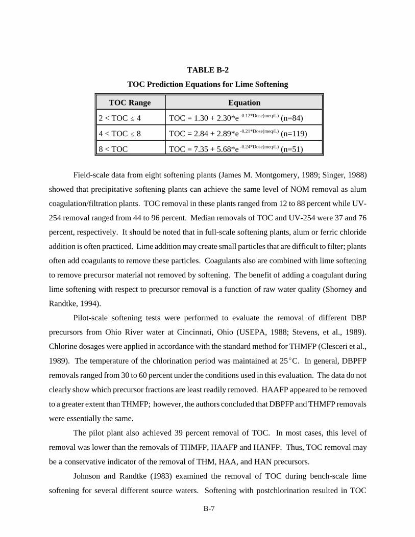
B-7

TABLE B-2

TOC Prediction Equations for Lime Softening

TOC Range Equation

2 < TOC � 4 TOC = 1.30 + 2.30*e -0.12*Dose(meq/L) (n=84)

4 < TOC � 8 TOC = 2.84 + 2.89*e -0.21*Dose(meq/L) (n=119)

8 < TOC TOC = 7.35 + 5.68*e -0.24*Dose(meq/L) (n=51)

Field-scale data from eight softening plants (James M. Montgomery, 1989; Singer, 1988)

showed that precipitative softening plants can achieve the same level of NOM removal as alum

coagulation/filtration plants. TOC removal in these plants ranged from 12 to 88 percent while UV-

254 removal ranged from 44 to 96 percent. Median removals of TOC and UV-254 were 37 and 76

percent, respectively. It should be noted that in full-scale softening plants, alum or ferric chloride

addition is often practiced. Lime addition may create small particles that are difficult to filter; plants

often add coagulants to remove these particles. Coagulants also are combined with lime softening

to remove precursor material not removed by softening. The benefit of adding a coagulant during

lime softening with respect to precursor removal is a function of raw water quality (Shorney and

Randtke, 1994).

Pilot-scale softening tests were performed to evaluate the removal of different DBP

precursors from Ohio River water at Cincinnati, Ohio (USEPA, 1988; Stevens, et al., 1989).

Chlorine dosages were applied in accordance with the standard method for THMFP (Clesceri et al.,

1989). The temperature of the chlorination period was maintained at 25(C. In general, DBPFP

removals ranged from 30 to 60 percent under the conditions used in this evaluation. The data do not

clearly show which precursor fractions are least readily removed. HAAFP appeared to be removed

to a greater extent than THMFP; however, the authors concluded that DBPFP and THMFP removals

were essentially the same.

The pilot plant also achieved 39 percent removal of TOC. In most cases, this level of

removal was lower than the removals of THMFP, HAAFP and HANFP. Thus, TOC removal may

be a conservative indicator of the removal of THM, HAA, and HAN precursors.

Johnson and Randtke (1983) examined the removal of TOC during bench-scale lime

softening for several different source waters. Softening with postchlorination resulted in TOC

B-8

reductions of 14 and 32 percent for a river water and groundwater, respectively. Softening with

postchlorination of a fulvic acid solution resulted in TOC reductions of 46, 85, and 92 percent for

lime doses of 100, 200, and 300 mg/L, respectively.

B.5 SUMMARY

Precipitative softening can achieve the same range of TOC removal as achieved by alum

coagulation/filtration processes. Field-scale data from eight softening plants showed that these

plants were achieving TOC removals of 12 to 88 percent and UV-254 removals of 44 to 96 percent.

Pilot-scale studies with Ohio River water showed that TOC removal may be a generally conservative

indicator of THMFP, HAAFP, and HANFP removal.

Like coagulation/filtration processes, the precipitative softening process can be modified to

increase NOM removal. In general, NOM removal is enhanced by conditions that favor the

formation of magnesium hydroxide and small calcium carbonate particles. These conditions are

achieved by:

& Elevating pH to approximately 10.8 or higher.& Delaying carbonate addition for several minutes.& Delaying sludge recycling.

The last two modifications inhibit the removal of hardness. Thus, process modifications

should be implemented cautiously. For systems employing a multi-staged process, satisfactory NOM

and hardness removal might be achieved by the two-stage process noted above. In many full-scale

cases, alum or ferric coagulants also are used.

Appendix C

OTHER DBP PRECURSOR REMOVAL TECHNOLOGIES

Table of Contents

Page

C.0 OTHER DBP PRECURSOR REMOVAL TECHNOLOGIES

C.1 Adsorption Processes . . . . . . . . . . . . . . . . . . . . . . . . . . . . . . . . . . . . . . . . C-1C.1.1 Granular Activated Carbon. . . . . . . . . . . . . . . . . . . . . . . . . . . . C-1C.1.2 Powdered Activated Carbon. . . . . . . . . . . . . . . . . . . . . . . . . . . C-5

C.2 Membranes . . . . . . . . . . . . . . . . . . . . . . . . . . . . . . . . . . . . . . . . . . . . . . . C-7

C-1

APPENDIX C

OTHER DBP PRECURSOR REMOVAL TECHNOLOGIES

C.1 ADSORPTION PROCESSES

C.1.1 Granular Activated Carbon

The application of granular activated carbon (GAC) adsorption for drinking water

treatment involves the following major process design considerations:

• Empty bed contact time (EBCT, volume of empty contactor divided by flow rate).

• Reactivation interval or frequency.

• GAC usage rate (pounds of GAC used per gallon of water treated).

• Pretreatment.

• Contactor configuration (e.g., downflow versus upflow, pressure versus gravity,single-stage versus multi-stage or parallel, filter adsorber versus post-filter GACcontactor).

• Method of GAC reactivation (e.g., on-site versus off-site).

The EBCT provides an indication of the quantity of GAC on-line at any one time, and

thus reflects the capital cost for the system. The EBCT is an important design parameter and

may have some impact on the GAC usage rate for removal of NOM.

GAC adsorption, as practiced in water treatment, is not a steady-state process, with

the effluent concentration increasing with time. Once the effluent concentration meets the

maximum allowable concentration for a contaminant, the GAC column must be taken off-

line and the GAC replaced with reactivated or fresh GAC. The operation time to this

maximum effluent concentration is termed the reactivation interval.

The GAC usage rate provides an indication of the rate at which the GAC is exhausted

or replaced and, therefore, primarily affects the operating cost of the GAC treatment system.

C-2

For a full-scale GAC installation, the GAC usage rate often dictates the choice between

providing an on-site reactivation system or replacing the spent GAC with virgin GAC. It

also affects the costs of GAC handling (i.e., storage, dewatering, attrition losses, and

transportation).

GAC systems may require some kind of pretreatment to prevent clogging of the GAC

bed, to minimize the organic loading on the GAC, and to improve cost effectiveness.

Clogging of the GAC bed could be caused by suspended solids in the raw water or by

precipitation of calcium carbonate, iron, and manganese on the GAC. Suspended solids

typically cause problems in surface water systems, while carbonate scaling and iron and

manganese precipitation may occur in both surface and ground waters. When the GAC bed

life is long, clogging may also be caused by biological growths. Pretreatment methods

include coagulation, filtration, or softening ahead of the GAC system. Conventional

coagulation, clarification, and filtration processes may be optimized for organics removal to

reduce natural organic loading to the GAC bed.

Based on the estimates of GAC usage rate and contact time, a conceptual process

design can be developed by evaluating various contactor configurations. The two basic

modes of contactor operation are downflow and upflow. Upflow beds typically have been

applied to situations where very long contact times (greater than 120 minutes) are required

and/or where the level of suspended solids is high. Downflow fixed bed contactors offer the

simplest and most common contactor configuration for drinking water treatment. The

contactors can be operated either under pressure or by gravity.

The choice of pressure or gravity is generally dependent upon the hydraulic

constraints of a given system. Pressure contactors may be more applicable to ground water

systems because pumping of the ground water is required. Gravity contactors are generally

more suitable for surface water systems if sufficient head is available. Gravity contactors,

when used, are typically placed downstream of surface water filtration systems.

GAC contactors may be operated in a series or parallel configuration. In a series

configuration, GAC in the first contactor is reactivated when the effluent of the second

contactor no longer meets the treatment objective. Once the GAC in the first contactor is

replaced, the roles of the two contactors may be reversed, where the second contactor

C-3

becomes the first contactor and vice versa. NOM is a mixture of unknown compounds which

separate along the bed in a manner proportional to their adsorption potential. Weakly

adsorbing components of NOM may irreversibly preload the GAC at the downstream end

of the bed and may, therefore, reduce the capacity of the bed for stronger adsorbing

components at the end of the bed.

In parallel operation, multiple GAC beds can be operated in a staggered pattern such

that effluents from beds with breakthrough concentrations higher than the treatment objective

are blended with effluents from beds with little or no breakthrough. In this manner, the

combined effluent concentration from the GAC beds can be kept less than the specified

treatment objective, and exhausted beds would be reactivated in a staggered manner.

The choice between a single contactor and contactors in series or parallel is site

specific and depends on the type and concentration of the contaminant to be removed and its

rate of adsorption. This choice also depends on the types, concentrations, and adsorption

rates of competing contaminants. Furthermore, an economic analysis should be performed

based on site specific data to decide on an optimal contactor configuration.

GAC contactors should be used when longer EBCTs are required, while filter-

adsorbers, where the top portion of the sand is replaced by GAC, can be used when shorter

EBCTs are feasible. Because of their short EBCTs, filter-adsorbers meet desired water

quality goals for a much shorter period of time than GAC contactors. For treating seasonal

changes in water quality or contaminant shock loads, filter-adsorbers may have an economic

advantage over post-filter GAC contactors. One disadvantage of filter-adsorbers is that GAC

losses are high during backwashing and reactivation, and equipment separating GAC from

sand may be required before reactivation. An economic analysis considering GAC usage rate

and treatment goals should be performed to decide between GAC contactor and filter-

adsorber modes of operation.

Another consideration in the design of a GAC system is the method of GAC

reactivation. The two basic approaches to regenerating GAC are:

• Off-site disposal or reactivation

• On-site reactivation.

C-4

Based on information from GAC manufacturers, on-site reactivation is not generally

economical for systems where the GAC usage rate is less than 2,000 lb/day.

Under the throwaway concept of off-site disposal, virgin GAC is generally purchased

in bags or drums. Once the GAC becomes exhausted, it is generally slurried by gravity to

a draining bin where the free water is removed and returned for treatment. The drained GAC

is then manually drummed and shipped for landfilling or incineration.

The advantage of this approach lies mainly in its technical simplicity. It is a sound

approach for applications requiring a relatively small GAC usage rate, generally less than 500

lb/day. The need to dispose of the spent GAC, however, is a definite drawback, especially

if testing demonstrates that the spent GAC is considered a hazardous waste. If this occurs,

it may become necessary to consider incineration of the spent GAC prior to disposal in a

landfill. Alternatively, a hazardous waste landfill could be used at increased cost.

The off-site reactivation approach is somewhat similar to the throwaway concept

from a GAC handling standpoint; however, it assumes some of the economies associated

with GAC reuse. When compared to other alternatives, however, the number of handling

steps and resulting GAC losses are a major disadvantage. The off-site reactivation approach

has generally proven most cost effective in applications where the GAC usage rate falls in

the 500 to 2,000 lb/day range (Kornegay, 1979).

The major equipment typically found in a GAC installation includes:

• GAC Contactors - either common wall concrete or lined steel vessels. In either case,provisions for underdrainage, backwashing, and removing the spent GAC must bemade.

• GAC Storage - additional storage facilities may be required for handling of virgin,reactivated, and spent GAC, depending on the type and size of the facility.

• GAC Transport Facilities - includes piping, valves, and pumps.

• GAC Fill - the actual initial GAC charge depends on the type and volume of GACrequired for treatment.

C-5

C.1.2 Powdered Activated Carbon

PAC has been successfully used for taste and odor control in many water treatment

facilities. PAC can also be used to remove NOM. The application of PAC for removal of

NOM from drinking water supplies involves the following major process design

consideration:

• PAC usage rate

• Contact time

• PAC disposal.

In typical water treatment situations, PAC is added at the rapid mix stage, along with

coagulants, and settles out in the sedimentation stage. The growth of floc around PAC

particles, however, may block adsorption onto PAC to some degree. Many studies have

indicated that PAC capacity for NOM increases with contact time up to seven days or longer.

Therefore, the contact time in conventional settling basins (typically several hours) may not

be long enough to produce effective removal of NOM by PAC.

Two different PACs, Westvaco Aqua Nuchar and Westvaco Nuchar SA, were studied

for precursor removal in conjunction with alum coagulation (Malcolm Pirnie 1988

unpublished data). Results indicate that alum coagulation alone achieved an average 55

percent reduction of THMFP. Alum coagulation combined with Aqua Nuchar dosed at 25

mg/L (0.21 lb/1,000 gal) reduced THMFP by 70 percent with preozonation (0.05 to 0.2 mg

03/mg TOC) and 60 percent without preozonation. Alum coagulation combined with Nuchar

SA dosed at 16 to 21 mg/L (0.13 to 0.18 lb/1,000 gal) reduced THMFP by 75 percent with

preozonation and 70 percent without preozonation. These dosages are significantly higher

than those typically used in drinking water treatment and represent a significant increase in

sludge production. With these relatively high dosages, PAC enhanced TOC removal by 10

to 20 percent and THMFP removal by 0 to 20 percent.

Two additional applications of PAC in water treatment include: (1) prior to an

upflow solids contact clarifier, and (2) in conjunction with low pressure membranes. An

upflow solids contact clarifier may retain PAC in the sludge blanket, significantly increasing

C-6

PAC contact time and capacity for NOM removal beyond that seen when PAC is simply

added to a point in the treatment train. Kassam et al. (1991) reported mean carbon residence

times in contact recirculating clarifiers from nine hours to 8.5 days. Hoehn et al. (1987) and

Najm et al. (1989) documented the addition of PAC to pilot-scale floc blanket reactors and

found PAC retention times of between nine hours and two days. Increasing PAC retention

time can significantly decrease the required dose. PAC dose was reduced by 25-40 percent

for the adsorption of a detergent (Najm et al., 1991).

PAC is often used with membrane processes. Combining PAC with membrane

filtration improves process performance in two ways: (1) organics removal is increased, and

(2) membrane fouling by organic absorption is decreased. Typically, low-pressure membrane

processes, such as microfiltration (MF) and ultrafiltration (UF), cannot remove a substantial

amount of organic material due to their relatively large pore size. PAC addition improves

NOM removal by associating NOM, which alone would pass through the pores, with the

filterable particulate phase. PAC combined with crossflow membrane processes can also

greatly increase the PAC detention time by recycling PAC through the membrane fibers.

Many PAC/UF studies have evaluated organic carbon removal (Anselme and Charles, 1990;

Laine et al., 1990; Heneghan and Clark, 1991; Adham et al., 1991; Adham et al., 1993;

Jacangelo, 1995; Marriott et al., 1997; Jack, 1997). TOC removals between 13 and 85

percent and DOC removals between 13 and 76 percent have been documented.

PAC can also reduce membrane fouling by preventing organics from adsorbing to the

membrane surface. This enhances membrane flux, reduces the frequency of chemical

cleanings, and prolongs the life of the membrane (Laine et al., 1990; Marriott et al., 1997;

Henegan and Clark, 1991; Jacangelo, 1995).

C-7

C.2 MEMBRANES

Membrane processes can remove DBP precursors through filtration and adsorption

of organics. If NOM molecules are larger than the membrane pores, NOM will be rejected

and DBPFP will be reduced. Size, however, is only one factor which influences NOM

rejection. Shape and chemical characteristics of organic compounds also play important

roles in the permeation of NOM through a membrane (AWWARF, 1996). Membranes may

also remove NOM through adsorption of organics on the membrane surface. Adsorption

depends on the chemical characteristics, particularly charge and hydrophobicity, of both the

membrane material and organic compounds. Unfortunately, organic adsorption is

undesirable since it has proven to be a primary cause of irreversible fouling.

Pressure-driven membrane processes are typically categorized into MF, UF,

nanofiltration (NF), and reverse osmosis (RO). High-pressure processes (i.e., NF and RO)

have a relatively smaller pore size allowing significant DBP precursor removal. Low-

pressure processes (i.e., MF and UF), however, have a relatively larger pore size and cannot

remove NOM substantially without pretreatment.

DBP precursor removal will be a function of the type of membrane process,

membrane material characteristics, and water quality characteristics (e.g., NOM

characterization and concentration, pH). Some major design considerations for the use of

membranes for the removal of DBP precursors include the following (Carlson, 1991):

• Removal efficiency of NOM.

• Preliminary treatment required to provide a satisfactory membrane feed water qualityand to limit membrane fouling.

• Frequency of fouling and recovery and NOM removal efficiency after repeatedfouling/cleaning cycles.

Without pretreatment, membrane processes remove NOM to varying degrees. MF

and UF removals typically range between about 5 and 30 percent. Typically NF and RO

removals are on the order of 50 to 99 percent. Membranes, particularly those with molecular

weight cutoffs (MWCOs) in the 100 to 500 range, appear to be very effective as a means of

C-8

DBP precursor removal. TOC, THMFP, and TOXFP removals of 70 to 95 percent are

commonly achieved in systems using such membranes. Larger MWCO membranes,

however, will not be as effective for these removals.

While MWCO is an important indicator of process performance, it is also an

important indicator of process costs. Systems using membranes with higher MWCOs are

likely to achieve higher product water flux and operate at lower pressures (and lower costs)

than those using membranes with lower MWCOs. In effect, improved effluent water quality

is traded for higher costs. Higher MWCO membranes can be combined with PAC or

coagulations to allow substantial DBP precursor removal. This increases costs as well.

However, with recent advances in membrane technology, increasing popularity, and the

threat of stricter regulations, membranes are becoming cost competitive with traditional

processes.

Appendix D

COAGULANT DOSAGES FOR STEP 2 TESTING

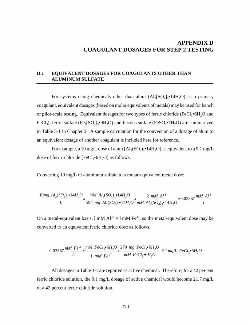
D-1

10mg Al2(SO4)3&14H2O

Lx

mM Al2(SO4)3&14H2O

594 mg Al2(SO4)3&14H2Ox

2 mM Al3�

mM Al2(SO4)3&14H2O³0.03367

mM Al3�

L

0.03367mM Fe3�

Lx

mM FeCl3&6H2O

1 mM Fe3�x

270 mg FeCl3&6H2O

mM FeCl3&6H2O³9.1mg/L FeCl3&6H2O

APPENDIX DCOAGULANT DOSAGES FOR STEP 2 TESTING

D.1 EQUIVALENT DOSAGES FOR COAGULANTS OTHER THAN ALUMINUM SULFATE

For systems using chemicals other than alum (Al2[SO4]3•14H2O) as a primary

coagulant, equivalent dosages (based on molar equivalents of metals) may be used for bench

or pilot-scale testing. Equivalent dosages for two types of ferric chloride (FeCl3•6H2O and

FeCl3), ferric sulfate (Fe2[SO4]3•9H2O) and ferrous sulfate (FeSO4•7H2O) are summarized

in Table 3-1 in Chapter 3. A sample calculation for the conversion of a dosage of alum to

an equivalent dosage of another coagulant is included here for reference.

For example, a 10 mg/L dose of alum [Al2(SO4)3•14H2O] is equivalent to a 9.1 mg/L

dose of ferric chloride [FeCl3•6H2O] as follows.

Converting 10 mg/L of aluminum sulfate to a molar-equivalent metal dose:

On a metal-equivalent basis, l mM Al3+ = l mM Fe3+, so the metal-equivalent dose may be

converted to an equivalent ferric chloride dose as follows.

All dosages in Table 3-1 are reported as active chemical. Therefore, for a 42 percent

ferric chloride solution, the 9.1 mg/L dosage of active chemical would become 21.7 mg/L

of a 42 percent ferric chloride solution.

Ref-1

REFERENCES

Adham, S., V.J. Snoeyink, M.M. Clark, and J-L. Bersillon, 1991. "Predicting and VerifyingOrganics Removal by PAC in an Ultrafiltration System." J. AWWA, 83:12:81.

Adham, S., V.J. Snoeyink, M.M. Clark, and C. Anselme, 1993. "Predicting and VerifyingOrganics Removal by PAC in Pilot-Scale UF Systems." J. AWWA, 85:12:58.

Amirtharajah, A., and C.R. O’Melia, 1990. “Coagulation Processes: Destabilization, Mixing,and Flocculation.” in: Water Quality and Treatment: A Handbook of CommunityWater Supplies. F.W. Pontius (ed.), McGraw-Hill, NY (fourth ed.).

Anselme, C., and P. Charles, 1990. "The Use of Powdered Activated Carbon for theRemoval of Specific Pollutants in Ultrafiltration processes." Laboratoire Central,Lyonnaise des Eaux, Le Pecq, France.

AWWARF (American Water Works Association Research Foundation), 1989. ProceduresManual for Polymer Selection in Water Treatment Plants, AWWA, Denver, CO.

AWWARF, 1990. Lead Control Strategies. AWWA Research Foundation and AWWA,Denver, CO.

AWWARF, 1991. Ozone in Water Treatment. Eds: Langlais, B., Reckhow, D.A., Brink, D.,Lewis Publishers, Chelsea, MI.

AWWARF and DVGW Forschungsstelle, 1985. Internal Corrosion of Water DistributionSystems. AWWA Research Foundation/DVGW-Forschungsstelle, Denver, CO.

AWWARF and KIWA (Keuringsinstituut voor Waterleidingartikelen), 1988. The Searchfor a Surrogate, AWWA, Denver, CO.

AWWARF, 1996. Water Treatment Membrane Processes. With Lyonnaise des Eaux, WaterResearch Commission of South Africa. McGraw Hill, NY.

AWWARF-TZW, 1996. Internal Corrosion of Water Distribution Systems. AWWAResearch Foundation/DVGW-TZW, Denver, CO, (Second ed.).

Bonacquisti, T.P., and E. Petrovitch, 1988. "Preoxidation Using Potassium Permanganateat the Fairfax County Water Authority." Presented at the 1988 Conf. Virginia SectionAWWA, Fairfax, VA.

Carlson, M., 1991. "Disinfection Byproducts Precursor Removal." Presented at the 1991Annual AWWA Conference, Philadelphia, PA.

REFERENCES (Cont'd)

Ref-2

Carlson, K.H., D. Gregory, S. MacMillan, 1996. “The Efficacy of Preozonation andEnhanced Coagulation for Treating Low Alkalinity, High Color Water.” Proc. 1996AWWA Annual Conference, Research Division, Toronto, Ontario.

Carlson, K.H., W.R. Knocke, K.R. Gertig, 1997. “Optimizing Treatment through Iron andManganese Fractionation.” J. AWWA, 89:4:56.

Chadik, P.A., and G.L. Amy, 1983. "Removing Trihalomethane Precursors from VariousNatural Waters by Metal Coagulants." J. AWWA, 75:10:532.

Chang, S.D., and P.C. Singer 1991. "The Impact of Ozonation on Particle Stability and theRemoval of TOC and THM Precursors." J. AWWA, 83:3:71.

Cheng, R.C., R.S. Yates, S.W. Krasner, and S. Liang, 1995. “Bench-Scale Evaluation of theEffects of Seasonal Change on TOC Removal by Enhanced Coagulation.” Proc. 1995AWWA Ann. Conf. (Water Quality), Anaheim, Calif.

Chowdhury, Z.K., J.A. Roberson, and D.M. Owen, 1997. “A National Evaluation ofEnhanced Coagulation and Enhanced Softening.” Proc. AWWA Annual Conference,Atlanta, GA, June 1997.

Clesceri, L.S., A.E. Greenberg, and R.R. Trussell, eds., 1989. Standard Methods for theExamination of Water and Wastewater. 17th Edition, AWWA, WPCF, APHA.

Collins, M.R., G.L. Amy, and P.H. King, 1985. "Removal of Organic Matter in WaterTreatment." J. Env. Eng., 111:6:850.

Colthurst, J.M., and P.C. Singer, 1982. "Removing Trihalomethane Precursors byPermanganate Oxidation and Manganese Dioxide Adsorption." J. AWWA, 74:2:78.

DeMarco, J., R. Miller, D. Davis, and C. Cole, 1983. "Experience in Operating a Full-ScaleGranular Activated Carbon System with On-Site Reactivation." in Treatment of Waterby Granular Activated Carbon, by M.J. McGuire and I.H. Suffet, eds., AmericanChemical Society, Washington, D.C.

Doré et al., 1988. “Interactions Between Ozone, Halogens, and Organic Compounds.”Ozone Sci. Eng., 10:153.

Duguet, J.P., E. Brodard, B. Dussert, and J. Mallevialle, 1985. “Improvement in theEffectiveness of Ozonation of Drinking Water through the Use of HydrogenPeroxide.” Ozone Sci. Eng., 7:241.

REFERENCES (Cont'd)

Ref-3

Edwards, M., 1997. “Predicting DOC Removal during Enhanced Coagulation.” J. AWWA,89:5:78.

Edwards, M., T.E. Meyer, J. Rehring, 1994. “Effect of Selected Anions on CopperCorrosion Rates.” J. AWWA, 85:10:105.

Edwards, M., M.R. Schock, and T.E. Meyer, 1996. “Alkalinity, pH and Copper CorrosionBy-product Release.” J. AWWA, 88:3:80.

Edwards, M., B. Courtney, P.S. Heppler, and M. Hernandez, 1997. “Recycling IronCoagulation Sludge by Discharge to Sewers.” ASCE Journal of EnvironmentalEngineering, October 1997.

Edzwald, J.K., W.C. Becker, and K.L. Wattier, 1985. “Surrogate Parameters for MonitoringOrganic Matter and THM Precursors.” J. AWWA, 77:4:122.

Edzwald, J.K., and J.E. Van Benschoten, 1990. “Aluminum Coagulation of Natural OrganicMatter.” Proc. 4th International Guthenburg Symposium on Chemical Treatment,Madrid, Spain, October, 1990.

El-Rehaili, A.M., and W.J. Weber, 1987. “Correlation of Humic Substance TrihalomethaneFormation Potential and Adsorption Behavior to Molecular Weight Distribution inRaw and Chemically Treated Waters.” Water Research, 21:5:573.

Ferguson, D.W., J.T. Gramith, and M.J. McGuire, 1991. “Applying Ozone for OrganicsControl and Disinfection: A Utility Perspective.” J. AWWA, 83:5:31.

Finch, G.R., L. Liyanage, and M. Belosovic, 1995. “Effect of Chlorine Dioxide on C.Parvum and G.Lamblia.” Proc. Chlorine Dioxide: Drinking Water, Process Water, andWastewater Issues, Third International Symposium. AWWARF, New Orleans, LA.

Fuge, R., N.J.G. Pearce, and W.T. Perkins, 1992. "Unusual Sources of Aluminum and HeavyMetals in Potable Waters." Environ. Geochem. and Health, 14:1:15.

Gramith, J.T., D.W. Furguson, and E.G. Means III, 1991. "Ozone and Perozone for Controlof Disinfection By-products: Metropolitan's Experience," presented at the 1991Annual AWWA Conference, Philadelphia, PA.

Hecht, P., 1993. "Effect of Optimizing the Removal of DBP Precursor Material on anExisting Residuals Management Program." Joint AWWA/WEF ResidualsManagement Conference, Phoenix, Arizona, December 1993.

REFERENCES (Cont'd)

Ref-4

Heneghan, K., and M. Clark, 1991. "Surface Water Treatment by Combined Ultrafiltration -PAC and Adsorption-Coagulation for Removal of Organics, Turbidity, and Bacteria."AWWA Specialty Conference on Membrane Technology, Orlando, Florida, March1991.

Hoehn, R.C., S.R. Laviner, C.Hamann Jr., E.R. Hoffman, J. McElroy, and E.G. Snyder,1987. “THM-Precursor Control with Powdered Activated Carbon in a Pulsed-Bed,Solids Contact Clarifier.” AWWA Ann. Conf., Kansas City, Mo., June, 1987.

Hubel, R.E., and J.K. Edzwald 1987. "Removing Trihalomethane Precursors by Coagulation." J. AWWA, 79:7:98.

Hudson, H.E., 1981. Water Clarification Processes: Practical Design and Evaluation. VanNorstrand Reinhold, New York.

Jacangelo, J.G., 1995. “UF with Pretreatment for Removing THM Precursors.” J. AWWA,87:3:100.

Jack, A., 1997. Performance and Optimization of a Combined Ultrafiltration/PAC Processfor Surface Water Treatment. MS Thesis, University of Illinois, Urbana-Champaign.

James M. Montgomery Consulting Engineers, Inc., 1985. Water Treatment Principles andDesign.

James M. Montgomery Consulting Engineers, Inc., 1992. Effect of Coagulation andOzonation on the Formation of Disinfection Byproducts. Prepared for the AWWA.

James M. Montgomery Consulting Engineers, Inc., 1989. Disinfection By-Products in U.S.Drinking Waters. USEPA and Association of Metropolitan Water Agencies.

Jekel, M.R., and B.U. Ernst, 1981. Einfluss von huminstoffen und ihrer ozonten produkteauf die electrotykoagulation von polystyrolatex.” Vom Wasser, 57:123.

Jodellah, A.A., and W.J. Weber, 1985. “Controlling Trihalomethane Formation Potentialby Chemical Treatment and Adsorption.” J. AWWA, 77:10:95.

Johnson, D.E., and S.J. Randtke, 1983. "Removing Non-Volatile Organic Chlorine and ItsPrecursors by Coagulation and Softening." J. AWWA, 75:5:249.

Kassam, L., P.M. Huck, A. van Roodselaar, and R. Shariff, 1991. “Accumulation andAdsorption Capacity of PAC in Slurry Recirculating Clarifier.” J. AWWA, 83:2:69.

REFERENCES (Cont'd)

Ref-5

Kavanaugh, M.C., 1978. "Modified Coagulation for Improved Removal of TrihalomethanePrecursors." J. AWWA, 70:11:613.

Kelkar, U., and G. Schafran, 1994. “Enhanced Coagulation: Impact on ResidualCharacteristics and Dewaterability.” AWWA Enhanced Coagulation ResearchWorkshop, Charleston, South Carolina, December 4-6.

Knocke, W.R., S. West, and R.C. Hoehn, 1986. "Effects of Low Temperature on theRemoval of Trihalomethane Precursors by Coagulation." J. AWWA, 78:4:189.

Knocke, W.R., J. Hamon, and B. Dulin, 1987. “Effects of Coagulation on SludgeThickening and Dewatering.” J. AWWA 79:6:89.

Knocke, W.R., and J. Van Benschoten, 1989. The Use of Various Oxidants for Control ofIron and Manganese in Water Treatment Facilities. AWWARF Report.

Knocke, W.R., J. Van Benschoten, M. Kearney, A. Soborski, and D. Reckhow, 1990a.Alternative Oxidants for the Removal of Soluble Iron and Manganese. AWWARFReport.

Knocke, W.R., R. Hungate, and S. Occiane, 1990b. Removal of Soluble Manganese fromWater by Oxide-Coated Media. AWWARF report.

Koch, B., S.W. Krasner, M.J. Sclimenti, and W.K. Schimpff, 1991. “Predicting theFormation of DBPs by the Simulated Distribution System.” J. AWWA, 83:10:62.

Kornegay, B.H., 1979. "Control of Synthetic Organic Chemicals of Activated Carbon:Theory, Application and Regeneration Alternatives." Presented at the Seminar onControl of Organic Chemicals in Drinking Water, sponsored by USEPA, Feb. 13-14,1979.

Korshin, G.V., S.A. Perry, J.F. Ferguson, 1996. “Influence of NOM on Copper Corrosion.”J. AWWA, 88:7:36.

Krasner, S.W., G. Amy, and H.W. Zhu, 1994. “Use of Some Simple NOM CharacterizationTechniques to Evaluate Enhanced Coagulation Treatability.” Proc. AWWAEnhanced Coagulation Research Workshop, Charleston, S.C. (Dec. 4-6, 1994).

Krasner, S.W., and G. Amy, 1995. “Jar-Test Evaluations of Enhanced Coagulation.” J.AWWA, 87:10:93.

REFERENCES (Cont'd)

Ref-6

Krasner, S.W., (and others), 1996. Issue paper prepared during USEPA TechnologiesWorking Group Meetings, January 1996.

Kriewall, D., 1996. "The Impact of Aluminum Residual on Transmission Main Capacity."Public Works, 127:12:28.

Laine, J-M., M.M. Clark, and J. Mallevialle, 1990. "Ultra Filtration of Lake Water: Effectof Pretreatment on the Partitioning of Organics, THMFP Flux." J. AWWA,82:12:82.

Lauer, W.C., and S.R. Lohman, 1994. "Non-Calcium Carbonate Protective Film LowersLead Values." Proc. AWWA Water Quality Technology Conference, San Francisco,CA, November 6-10 (1994).

Liao, M.Y., and S.J. Randtke, 1985. “Removing Fulvic Acid by Lime Softening.” J.AWWA, 77:8:78.

Logsdon, G.S., M.M. Frey, T.D. Stefanich, S.L. Johnson, D.E. Feely, J.B. Rose, and M.Sobsey, 1994. The Removal and Disinfection Efficiency of Lime SofteningProcesses for Giardia and Viruses. AWWA Research Foundation.

MacCarthy, P., and I.H. Suffet, 1989. "Introduction: Aquatic Humic Substances and TheirInfluence on the Fate and Treatment of Pollutants." in Aquatic Humic Substances:Influence on Fate and Treatment of Pollutants, I.H. Suffet and P. MacCarthy (eds.),American Chemical Society, Washington, DC.

Marriott, W.D., M.M. Clark, and J-M. Laine, 1997. “Piloting for Optimal Operation ofUltrafiltration.” Proc. Annual AWWA Membrane Conference, New Orleans, 1997.

Mays, L.M. (ed.), 1996. Water Resources Handbook. McGraw Hill, NY.

McGuire, M.J., M.K. Davis, S. Liang, C.H. Tate, E.M. Aieta, I.E. Wallace, D.R. Wilkes, J.C.Crittenden, and K. Vaith, 1989. Optimization and Economic Evaluation of GranularActivated Carbon for Organic Removal. AWWA, Denver, CO.

REFERENCES (Cont'd)

Ref-7

McTigue, N., 1995. “The Impact of Enhanced Coagulation on Residuals ManagementIssues.” Proc. WEF/AWWA Joint Residuals/Biosolids Conference, Kansas CityMissouri.

Merkle, P.B., W.R. Knocke, and D.L. Gallagher, 1997. “Method for Coating Media withSynthetic Manganese Oxide.” J. Envir. Engineering, ASCE, 123:7:642.

Munch, D.J. and D.P. Hautman, 1995. Method 551.1: Determination of ChlorinationDisinfection Byproducts, Chlorinated Solvents, and HalogenatedPesticides/Herbicides in Drinking Water by Liquid-Liquid Extraction and GasChromatography with Electron-Capture Detection. Revision 1.0, USEPA, NationalExposure Research Laboratory, Cincinnati, Ohio (1995).

Munch, D.J., J.W. Munch, and A.W. Pawlecki, 1995. Method 552.2: Determination ofHaloacetic Acids and Dalapon in Drinking Water by Liquid-Liquid Extraction,Derivatization and Gas Chromatography with Electron Capture Detection. Revision1.0, USEPA, National Exposure Research Laboratory, Cincinnati, Ohio (1995)

Najm, I.N., V.L. Snoeyink, M.T. Suidan, and Y. Richard, 1989. “Powdered ActivatedCarbon in Floc Blanket Reactors.” Proc. Annual AWWA Conference, Los Angeles,June 1989.

Najm, I.N., V.L. Snoeyink., B.W. Lykins Jr., and J.Q. Adams., 1991. “Using PowderedActivated Carbon: A Critical Review.” J. AWWA, 83:1:65.

Owen, D.M., G.L. Amy, and Z.K. Chowdhury, 1993. “Characterization of Natural OrganicMatter and its Relationship to Treatability.” AWWARF Report.

Owen, D.M., R.S. Summers, Z.K. Chowdhury, 1996. “Removal of DBP Precursors byGranular Activated Carbon Adsorption.” AWWARF Report.

Pontius, F.W., 1997. “Future Directions in Water Quality Regulations.” J. AWWA, 89:2:40.

Randtke, S.J., 1988. "Organic Contaminant Removal by Coagulation and Related ProcessCombinations." J. AWWA, 80:5:40.

REFERENCES (Cont'd)

Ref-8

Randtke, S.J., C.E. Thiel, M.Y. Liao, and C.N. Yamaya, 1982. “Removing Soluble OrganicContaminants by Lime-Softening.” J. AWWA, 74:4:192.

Reckhow, D.A., and P.C. Singer, 1984. "The Removal of Organic Halide Precursors byPreozonation and Alum Coagulation." J. AWWA, 76:4:151.

Rice, R.G., 1992. U.S. Potable Water Treatment Plants Using Ozone. RICE, Ashton, MD(Aug.-Sept. 1992).

Schock, M.R., 1990. "Internal Corrosion and Deposition Control.” in: Water Quality andTreatment: A Handbook of Community Water Supplies. F.W. Pontius (ed.),McGraw-Hill, NY (fourth ed.).

Schock, M.R., D. Lytle, and R. Miltner, 1994. “The Impact of Enhanced Coagulation onCorrosion Control and Inorganic Constituents in Drinking Water.” AWWAEnhanced Coagulation Research Workshop, Charleston, South Carolina, December4-6.

Semmens, M.J., and T.K. Field, 1980. "Coagulation: Experiences in Organics Removal."J. AWWA, 72:8:476.

Semmens, M.J., and A.B. Staples, 1986. "The Nature of Organics Removed DuringTreatment of Mississippi River Water." J. AWWA, 78:2:76.

Singer, P.C., 1988. Alternative Oxidant and Disinfectant Treatment Strategies forControlling Trihalomethane Formation. USEPA Risk Reduction EngineeringLaboratory, Cincinnati, OH. Rpt. No. EPA/600/2-88/044, NTIS Publ. No. PB88-238928.

Singer, P.C., J.H. Borchardt, and J.M. Colthurst, 1980. "The Effects of PermanganatePretreatment on Trihalomethane Formation in Drinking Water." J. AWWA,72:10:573.

Singer, P.C., and S.D. Chang, 1988. "Characterization of the Impact of Pre-Ozonation ofRaw Drinking Water." Presented at the 1988 Spring Technical Conference of theInternational Ozone Assoc., Monroe, MI.

REFERENCES (Cont'd)

Ref-9

Snoeyink, V.L., 1991. “Corrosion Characteristics of Materials.” Proc. National Workshopon Control of Lead and Copper in Drinking Water, Chicago, IL, September 23-25,1991.

Standard Methods for the Examination of Water and Wastewater, 19th ed., 1995. APHA,AWWA, WEF.

Steinberg, C., and U. Muenster, 1985. "Geochemistry and Ecological Role of HumicSubstances in Lakewater." in: Humic Substances in Soil, Sediment, and Water:Geochemistry, Isolation and Characterization, G.R. Aiken, et al., (eds.), Wiley-Interscience, New York, NY.

Stevens, A.A., and J.M. Symons, 1977. “Measurement of Trihalomethane and PrecursorConcentration Changes.” J. AWWA, 69:10:546.

Stevens, A.A., L.A. Moore, and R.J. Miltner, 1989. "Formation and Control of Non-Trihalomethane By-Products." J. AWWA, 81:8:54.

Summers, R.S., S.M. Hooper, H.M. Shukairy, G. Solarik, and D. Owen, 1996. “AssessingDBP Yield: Uniform Formation Conditions.” J. AWWA, 88:6:80.

Summers, R.S., G. Solarik, V.A. Hatcher, R.S. Isabel, and J.F. Stile, 1997. “Analyzing theImpacts of Predisinfection Through Jar Testing.” Proc. AWWA Water TechnologyConference, Denver, CO.

Symons, J.M., S.W. Krasner, L.S. Simms, and M. Sclimenti, 1993. “Measurement of THMand Precursor Concentrations Revisited: The Effect of Bromide Ion.” J. AWWA,85:1:51.

Symons, J.M., R. Xia, G.E. Seitel Jr., A.C. Diehl, C.J. Hwang, S.W. Krasner, and S.E.Barrett, 1998. Factors Affecting Disinfection By-Product Formation DuringChloramination. AWWA Research Foundation.

Tate, C.H., 1991. “Survey of Ozone Installations in North America.” J. AWWA, 83:5:40.

REFERENCES (Cont'd)

Ref-10

USEPA, 1988. In-House Pilot Studies for Control of Chlorination By-Products. OrganicsControl Branch, Drinking Water Research Division, Risk Reduction EngineeringLaboratory, Cincinnati, OH.

Vrijenhoek, E.M., A.E. Childress, M. Elimelech, T.S. Tanaka, and M.D. Beuhler, 1998.“Removing Particles and THM Precursors by Enhanced Coagulation.” J. AWWA,90:4:139.

Wallace, J.L., B. Vahadi, J.B. Fernandez, and B.H. Boyden, 1988. “Combination ofOzone/Hydrogen Peroxide and Ozone/UV Radiation for Reduction ofTrihalomethane Formation Potential in Surface Water.” Ozone: Science andEngineering, 10:1:103.

Weber, W.J. Jr., and A.M. Jodellah, 1985. “Removing Humic Substances by ChemicalTreatment and Adsorption.” J. AWWA, 77:4:132.

Werdehoff, K.S., and P.C. Singer, 1987. "Chlorine Dioxide Effects on THMFP, TOXFP,and the Formation of Inorganic By-Products." J. AWWA, 79:9:107.

Westerhoff, G., and Z.K. Chowdhury, 1996. “Water Treatment Systems.” A chapter inWater Resources Handbook. L.M. Mays (ed.), McGraw Hill, NY.

White, M.C., J.D. Thompson, G.W. Harrington, and P.C. Singer, 1997. “Evaluating Criteriafor Enhanced Coagulation Compliance.” J. AWWA, 89:5:64.

Young, J.S., and P.C. Singer, 1979. “Chloroform Formation in Public Water Supplies: ACase Study.” J. AWWA, 71:12:87.

Documents

Enhanced Coagulation and Enhanced Precipitative · PDF fileEnhanced Coa gulation and Enhanced Precipitative ... 4-3 DBP Precursor Removal Compliance Calculations for ... Settled Water