Enhanced 3D MIMO Channel for Urban M acro Environment · In the process of performance evaluation, the channel model plays an important role. The channel model has to reflect the

Enhanced 3D MIMO Channel for Urban Macro Environment

Dr.C.Arunachalaperumal, S.Dhilipkumar and G.Abija

[email protected], [email protected], [email protected]

Department of Electronics and Communication Engineering, SAEC

Abstract In order to design efficient MIMO communication systems and to understand the performance limits, it is necessary to understand the nature of the MIMO channel. Unlike wired channels, radio channels are extremely random and require complex analysis. Hence, channel modeling is an important and fundamental process required to evaluate the performance of any communication system. The modeling of MIMO channels is a multistep procedure. If realistic modeling is wanted, it must be based on MIMO measurements from which the relevant features are extracted. Significant determinants are the correlations between the transmission coefficients and the number of scatterers. Assuming more general randomness, a simulation model may be required to satisfy the experimental conditions only approximately in order to simplify matters. It is a common approximation to assume random phases from scatterers, in which case summation from a few scatterers leads to the well-known complex Gaussian distributions with Rayleigh distributions for the amplitudes. Another lesson learned from experiments is the clustering of rays in delay and angle. Such features have also been utilized in models.

Keywords- MIMO, CHANNEL MODELLING, SCM, SCME, WINNER, QuaDRiGa 1 1.

1OVERVIEW OF MIMO CHANNEL MODELS

1.1.General Classification

For a MIMO communication system, the characteristics of propagation of electromagnetic waves have to be described for all transmit and receive antenna pairs. Several channel models have been proposed for MIMO communication systems. The major categories of MIMO channel model are [1], [2]

1.Deterministic Channel Model i. Recorded Impulse Response [3], [4].

ii. Ray Tracing Technique[5]-[7].

2.Stochastic Channel Model i.Geometrically Based[8]

ii.Parametric Based {9], [10] iii.Correlation Based[11]-[13]

In deterministic channel modeling, deterministic predictions are used instead of field trial measurements to model the radio wave propagation. Stochastic channel modeling relies on the time varying, fading properties of the received signals, which are usually described by stochastic processes.

International Journal of Pure and Applied MathematicsVolume 118 No. 10 2018, 259-269ISSN: 1311-8080 (printed version); ISSN: 1314-3395 (on-line version)url: http://www.ijpam.eudoi: 10.12732/ijpam.v118i10.67Special Issue ijpam.eu

259

2. MIMO Channel Models for Simulations

The channel models computer simulation enables us to the evaluate the performance of MIMO wireless communication system. For designing, evaluating and analyzing the MIMO communication systems, the channel models should be capable of predicting both spatial and temporal characteristics of multipath signals. This section describes some of the channel models which have served to the system level simulations.

2.1. Spatial Channel Model for MIMO Simulations

The (SCM) Spatial Channel Model was developed within the 3rd

Generation Partnership Project group (3GPP

TM). The Spatial Channel Model is based on the Ray Tracing method of channel modeling.

Various wireless MIMO propagation scenarios can be simulated using the Spatial Channel Model. The model was implemented in MATLAB can be utilize the model to perform MIMO simulations .In SCM each resolvable path is characterized by its own spatial channel parameters such as angle spread, angle of arrival, power azimuth spectrum etc. All paths are assumed independent and these assumptions are applicable to both the BS and the MS specific spatial parameters. The details given here are based on the information available in the technical report produced by ETSI 3

rd Generation Partnership Project

group [14] .

2.1.1. Spatial Channel Parameters

SCM supports different channel environments like, the Suburban Macrocell, the Urban Macrocell and the Urban Microcell. The Macrocell scenarios have statistical similarities and follow the same modelling process with few parameter adjustments. For the Macrocell environments the adopted pathloss model is the modified COST231 Hata urban propagation model and for the Microcell environments the adopted pathloss model is the COST 231 Walfish-Ikegami NLOS model. As SCM uses a ray-based method. Each ray is described by its power and delay and can be decomposed to a large number of sub paths. The sub-rays that belong to the same ray have common powers and delays. If a „drop‟ is defined as a single simulation run where a BS using an array of S elements transmits inside a terrestrial environment to a moving MS using an array of U elements for a given number of time frames, the signal arrives to the receiver through N independent paths are described by their powers and delays. The channel is realized as,

( ) ∑ ∫ ( )

( ) (1)

( ) [

( ) ( )

( ) ( )

](2)

The main goal is to generate the channel coefficients, ( ) ( ) for every

( ) ( ) for every time frame.

2.2. Extended Spatial Channel Model (SCME)

SCME is an extension of SCM developed by the ETSI 3rd

Generation Partnership Project (3GPP). But the extension is not associated with the 3GPPworking group and was developed in WP5 of the WINNER – Wireless World Initiative New Radio project. In SCME the bandwidth has extended from

International Journal of Pure and Applied Mathematics Special Issue

260

5MHz to 20MHz. It was adopted as the channel standard for the development and testing of 3GPP Long Term Evolution (LTE) standard.[15], [16].

2.3. WINNER II Channel Model

The European Wireless World Initiative New Radio (WINNER) project group presented a simplified SCME Tap Delay-Line Model, portions of this model have been adopted by the 3GPP. In which, the specific AoDs and AoAs are specified and fixed for every path. The delays were selected to optimize the frequency decorrelation characteristic. However, in spite of the modification, the initial models were not adequate for the advanced WINNER I simulations. Therefore, new measurement-based models were developed and WINNER I generic model was created. The generic model is ray-based double-directional multi-link model that is antenna independent, scalable and capable of modeling channels for MIMO connections. WINNER I channel models were based on channel measurements performed at 2 and 5 GHz bands during the project. The models covered the following propagation scenarios specified in WINNER I: indoor, typical urban micro-cell, typical urban macro-cell, sub-urban macro-cell, rural macro-cell and stationary feeder link.

The WIM2 channel model (also referred to as WINNER II, 2006) is defined for both link-level and system-level simulations for a wide range of scenarios relevant to local, metropolitan and wide-area systems. WIM2 evolved from the WINNER I and WINNER II (interim) channel models.WIM2 is a double-directional geometry-based stochastic channel model. It incorporates generic multilink models for system-level simulations and clustered delay line (CDL) models, with fixed large-scale channel parameters. For each channel snapshot the channel parameters are calculated from the distributions. Channel realisations are generated by summing contributions of rays with specific channel parameters like delay, power, angle-of-arrival and angle-of-departure. Different scenarios are modelled by using the same. The models can be applied not only to WINNER II system, but also any other wireless system operating in 2 – 6 GHz frequency range with up to 100 MHz RF bandwidth. The models supports multi-antenna technologies, polarisation, multi-user, multi-cell, and multi-hop networks.

The channel from Tx antenna element s to Rx antenna element u for cluster n is,

( ) ∑ [ ( )

( )] *

+

[ ( )

( )] (

( ))

( ( )) ( ( )) (3)

where Frx,u,V and Frx,u,Hare the antenna element u field patterns for vertical and horizontal polarisations respectively, and are the complex gains of vertical-to-vertical and horizontal-to-vertical

polarisations of ray n,m respectively. Further 0 is the wave length of carrier frequency, is AoD

unitvector, is AoA unit vector, , and , are the location vectors of element s and u respectively, and τn,m is the Doppler frequency component of ray n,m.

2.4. WINNER + Channel Model

The WINNER + channel model is an extension of the WINNER II channel model to the three dimensional (3D) case [17]. The generalization from 2 to 3D is based on similar principles as generating the elevation angles as are used for the azimuth angles. The generic WINNER+ Final channel model follows a geometry-based stochastic channel modelling approach, which allows creating of an arbitrary double directional radio channel model. The channel models are antenna independent and the channel parameters are determined stochastically, based on statistical distributions extracted from channel measurements [18] . The small-scale parameters elevation at BS and UT are assumed Laplacian. It is enough to specify the standard deviation of SS elevation at BS and UT. For each channel


261

snapshot the channel parameters are calculated from the distributions. Channel realizations are generated by summing contributions of rays with specific channel parameters like delay, power, angle-of-arrival and angle-of-departure, now assuming that the departure and arrival angles include both azimuth and elevation.

2.5. QuaDRiGa

The QuaDRiGa (Quasi Deterministic Radio Channel Generator) channel model has been evolved from the WINNER II channel model described in WINNER II deliverable D1.1.2.v.1.1. This model follows a geometry-based stochastic channel modelling approach. This channel model is also antenna independent. The channel parameters are determined stochastically, based on statistical distributions extracted from channel measurements [19]. Specific channel realizations are generated by summing contributions of rays with specific channel parameters like delay, power, AoA and AoD. The main features of QuaDRiGa are:

Three Dimensional Propagation

Continuous Time Evolution Spatially correlated propagation parameter maps

Transitions between varying propagation scenarios

3. Simulation of 3D MIMO Channel Model

3.1. 3D Spatial Channel Modeling Approach

The propagation of electromagnetic signals rely on the spatial characteristics between the transmitter and the receiver. In the process of performance evaluation, the channel model plays an important role. The channel model has to reflect the exact scenario or the surrounding environment also the characteristics of electromagnetic signals can be realized in a better manner if three dimensional approach is utilized. The proposed channel model has been developed based on the concepts of recently developed channel models [20] .Most of the 3D channel models are based on Double Directional channel model in which the channel coefficients are determined from the knowledge of delays, angle of departure and angle of arrival. In 3D channel modelling determination of elevation angle is a challenging one. When elevation angle is considered, the equation 2.10 can be rewritten [21] as,

( ) √ ∑ [ ( )

( )]

[ (

) √ ( )

√ ( ) (

)]

[ ( )

( )] (

( )) ( ( ))

( ( )) (4)

Where, Frx,u,V and Frx,u,H are the antenna element u field patterns for vertical and horizontal polarizations respectively. Further 0 is the wave length of carrier frequency, is AoD

unitvector, is AoA unit vector, , and , are the location vectors of element s and u respectively, and τn,mis the Doppler frequency component of ray n,m. The Doppler frequency component is given as,

| | | |

(5)

In the proposed scheme the azimuth and elevation angles are obtained as the average of the angles calculated in Quadriga channel model and in the Method of Equal Volume. The cluster path is split into 20 sub-paths and the cluster angular spreads have been emulated. The azimuth/elevation angle of departure (AAoD/EAoD), (i.e., αT, βT), and azimuth/elevation angle of arrival (AAoA/EAoA), (i.e., αR, βR) in Two Sphere model are independent for double-bounced rays, while are correlated for single-


262

bounced rays. According to geometric algorithms, for the single-bounced rays resulting from the two-sphere model, one can derive the relationship between the AoDs and AoAs as αR≈π− RT/d sin αT, βR≈arccos(d−RTcos βT

(1)cosα T

(1))/ξn1, and αT≈ RR/d sinαR,βT≈arcos(d+RRcosβRcos αR)/ξn2 [20]. The

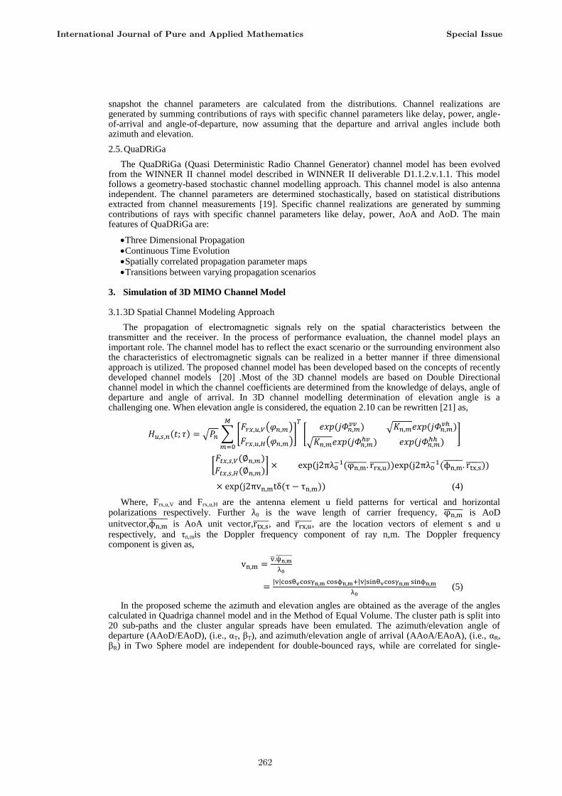
correlation factor used to determine the azimuth and elevation angles using inverse Gaussian function is obtained by taking the influence of K-factor and the number of clusters into account.

Figure 1. 3D Channel modeling approach in the proposed scheme

There are seven Large Scale Parameters similar to WINNER channel model. They are,

i)RMS Delay Spread (DS), ii)Ricean K-Factor (K or KF), iii) Shadow Fading (SF), iv)Azimuth Spread of Departure (AsD), v) Azimuth Spread of Arrival (AsA), vi)Elevation Spread of Departure (EsD), vii)Elevation Spread of Arrival (EsA)

In WINNER the maps are generated by filtering random, normal distributed numbers along the x and y axis of the map. Quadriga extends this idea by filtering the maps also in the diagonal directions and it helps to attain smoothness on the parameters over the trajectory.

3.2. Simulation Data Flow 1. Select the Scenario (urban Macro) 2. Set the Layout (No. of Transmitters & Receivers 3. Define the Antenna Parameters (No. of elements & Field Pattern) 4. Define the Antenna Orientation (Transmitters & Receivers) 5. Define the Characteristics of Mobile Terminal (Velocity & Movement) 6. Define the Simulation Parameters (Carrier frequency, Sample density, No. of Snapshots, etc.)

Φn,m

ΦdLOS

θaNLOS

θaLOS

LOS Path

Length dR0

NLOS Path

Length d1

Transmitter

Receiver

θLOS

θn,m CΦ

d

Cθ

βT

αT

βR αR

RT

RR

ζn1

ζn2


263

7. Assign Propagation conditions (No. of Drops and Tracks) 8. Calculate the Path Loss and Generate Correlated LSPs Define the Network Layout (No. of

Transmitters & Receivers) 9. Calculate Delays and Cluster Powers &Determine Azimuth and Elevation Angles. 10. Obtain XPR for each Receiver. 11. Draw Random initial phases and Generate Channel Coefficients. 12. Apply path loss, K-Factor and Shadow fading & Analyze or Post process according to the

requirements.

First the scenario has to be selected and the network layout has to be defined. The modellingapproach is based on the Quadriga Radio Channel Model. Data flow describes the steps or procedures involved in the simulation. The channel coefficients are generated at constant sampling rate.

3.3. Simulation Parameters

The simulation is carried out in three different channel modeling approaches. The same parameters are used for the simulation purpose for all channel models. The proposed channel model is Quadriga based 3D channel model while the other two models are the conventional channel models (SCM & WINNER II). The following parameters have been used for simulation.

Scenario Used : Urban Macro

Carrier Frequency : 5 GHz

No. of Sub-paths : 20

No. of Clusters : 20

No. of Snapshots : 49

Antenna Array : ULA4

Time Duration of Drop : 0.1Sec.

Samples per meter : 48

Velocity of MS : 60 Km/H

Maximum Distance : 2500 m

Height : 25/1.5 m

4. Simulation Results of 3D Channel Model

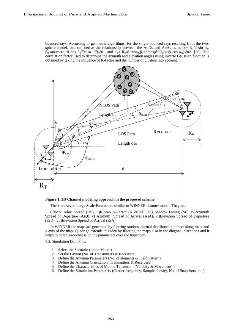
The proposed channel model mainly relies on the QuaDRiGa model in which the channel builder generates channel coefficients. It takes the correlated large scale parameters as inputs and determines the Channel Impulse Response (CIR) for each and every location. In addition to the azimuth angles elevation angles also calculated for every cluster

Figure.2 Path Loss Vs Distance (Theoretical)


264

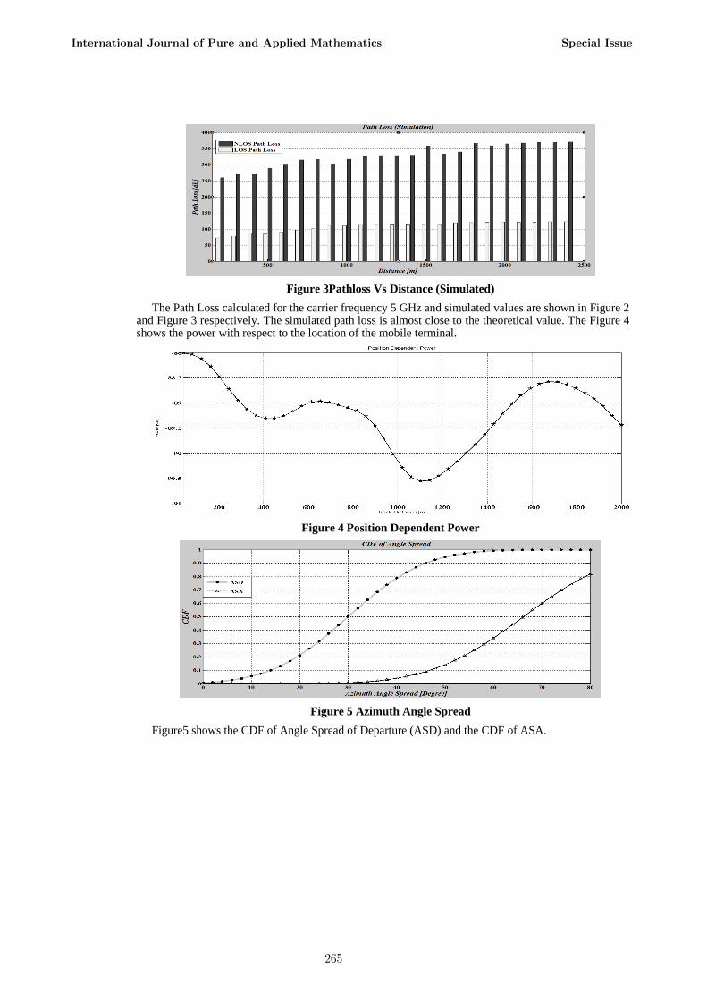
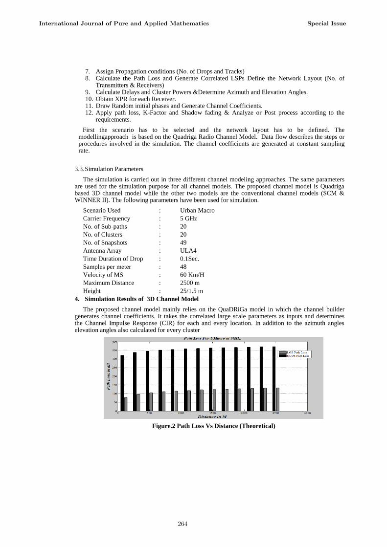
Figure 3Pathloss Vs Distance (Simulated)

The Path Loss calculated for the carrier frequency 5 GHz and simulated values are shown in Figure 2 and Figure 3 respectively. The simulated path loss is almost close to the theoretical value. The Figure 4 shows the power with respect to the location of the mobile terminal.

Figure 4 Position Dependent Power

Figure 5 Azimuth Angle Spread

Figure5 shows the CDF of Angle Spread of Departure (ASD) and the CDF of ASA.


265

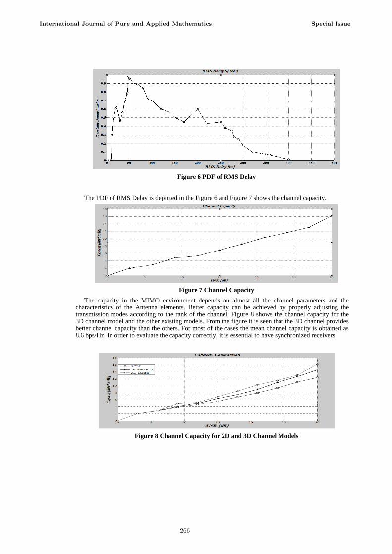
Figure 6 PDF of RMS Delay

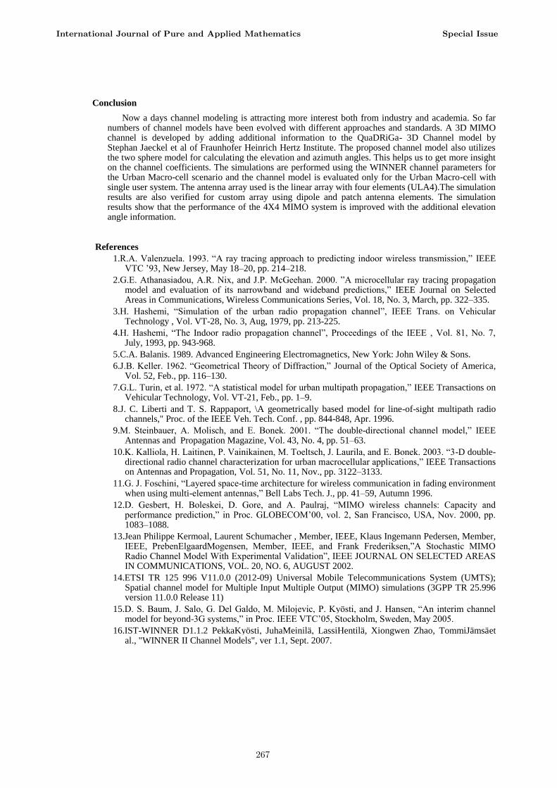
The PDF of RMS Delay is depicted in the Figure 6 and Figure 7 shows the channel capacity.

Figure 7 Channel Capacity

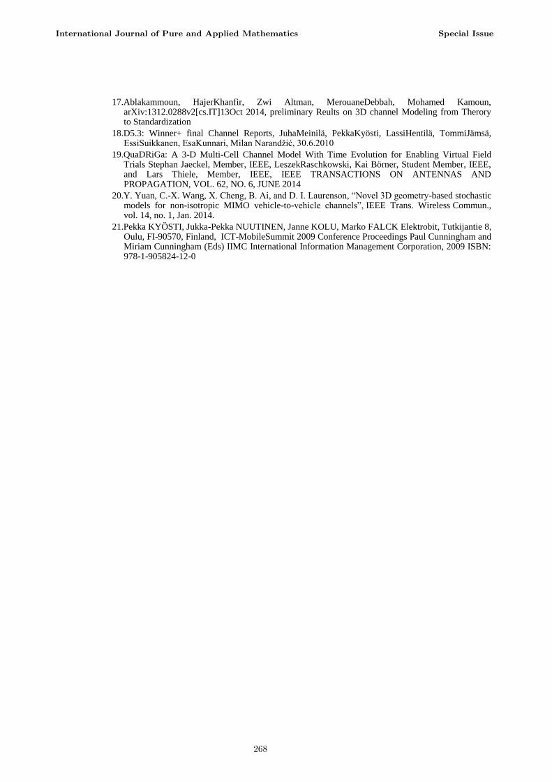
The capacity in the MIMO environment depends on almost all the channel parameters and the characteristics of the Antenna elements. Better capacity can be achieved by properly adjusting the transmission modes according to the rank of the channel. Figure 8 shows the channel capacity for the 3D channel model and the other existing models. From the figure it is seen that the 3D channel provides better channel capacity than the others. For most of the cases the mean channel capacity is obtained as 8.6 bps/Hz. In order to evaluate the capacity correctly, it is essential to have synchronized receivers.

Figure 8 Channel Capacity for 2D and 3D Channel Models


266

Conclusion

Now a days channel modeling is attracting more interest both from industry and academia. So far numbers of channel models have been evolved with different approaches and standards. A 3D MIMO channel is developed by adding additional information to the QuaDRiGa- 3D Channel model by Stephan Jaeckel et al of Fraunhofer Heinrich Hertz Institute. The proposed channel model also utilizes the two sphere model for calculating the elevation and azimuth angles. This helps us to get more insight on the channel coefficients. The simulations are performed using the WINNER channel parameters for the Urban Macro-cell scenario and the channel model is evaluated only for the Urban Macro-cell with single user system. The antenna array used is the linear array with four elements (ULA4).The simulation results are also verified for custom array using dipole and patch antenna elements. The simulation results show that the performance of the 4X4 MIMO system is improved with the additional elevation angle information.

References

1.R.A. Valenzuela. 1993. “A ray tracing approach to predicting indoor wireless transmission,” IEEE VTC ‟93, New Jersey, May 18–20, pp. 214–218.

2.G.E. Athanasiadou, A.R. Nix, and J.P. McGeehan. 2000. ”A microcellular ray tracing propagation model and evaluation of its narrowband and wideband predictions,” IEEE Journal on Selected Areas in Communications, Wireless Communications Series, Vol. 18, No. 3, March, pp. 322–335.

3.H. Hashemi, “Simulation of the urban radio propagation channel”, IEEE Trans. on Vehicular Technology , Vol. VT-28, No. 3, Aug, 1979, pp. 213-225.

4.H. Hashemi, “The Indoor radio propagation channel”, Proceedings of the IEEE , Vol. 81, No. 7, July, 1993, pp. 943-968.

5.C.A. Balanis. 1989. Advanced Engineering Electromagnetics, New York: John Wiley & Sons.

6.J.B. Keller. 1962. “Geometrical Theory of Diffraction,” Journal of the Optical Society of America, Vol. 52, Feb., pp. 116–130.

7.G.L. Turin, et al. 1972. “A statistical model for urban multipath propagation,” IEEE Transactions on Vehicular Technology, Vol. VT-21, Feb., pp. 1–9.

8.J. C. Liberti and T. S. Rappaport, \A geometrically based model for line-of-sight multipath radio channels," Proc. of the IEEE Veh. Tech. Conf. , pp. 844-848, Apr. 1996.

9.M. Steinbauer, A. Molisch, and E. Bonek. 2001. “The double-directional channel model,” IEEE Antennas and Propagation Magazine, Vol. 43, No. 4, pp. 51–63.

10.K. Kalliola, H. Laitinen, P. Vainikainen, M. Toeltsch, J. Laurila, and E. Bonek. 2003. “3-D double-directional radio channel characterization for urban macrocellular applications,” IEEE Transactions on Antennas and Propagation, Vol. 51, No. 11, Nov., pp. 3122–3133.

11.G. J. Foschini, “Layered space-time architecture for wireless communication in fading environment when using multi-element antennas,” Bell Labs Tech. J., pp. 41–59, Autumn 1996.

12.D. Gesbert, H. Boleskei, D. Gore, and A. Paulraj, “MIMO wireless channels: Capacity and performance prediction,” in Proc. GLOBECOM‟00, vol. 2, San Francisco, USA, Nov. 2000, pp. 1083–1088.

13.Jean Philippe Kermoal, Laurent Schumacher , Member, IEEE, Klaus Ingemann Pedersen, Member, IEEE, PrebenElgaardMogensen, Member, IEEE, and Frank Frederiksen,”A Stochastic MIMO Radio Channel Model With Experimental Validation”, IEEE JOURNAL ON SELECTED AREAS IN COMMUNICATIONS, VOL. 20, NO. 6, AUGUST 2002.

14.ETSI TR 125 996 V11.0.0 (2012-09) Universal Mobile Telecommunications System (UMTS); Spatial channel model for Multiple Input Multiple Output (MIMO) simulations (3GPP TR 25.996 version 11.0.0 Release 11)

15.D. S. Baum, J. Salo, G. Del Galdo, M. Milojevic, P. Kyösti, and J. Hansen, “An interim channel model for beyond-3G systems,” in Proc. IEEE VTC‟05, Stockholm, Sweden, May 2005.

16.IST-WINNER D1.1.2 PekkaKyösti, JuhaMeinilä, LassiHentilä, Xiongwen Zhao, TommiJämsäet al., "WINNER II Channel Models", ver 1.1, Sept. 2007.


267

17.Ablakammoun, HajerKhanfir, Zwi Altman, MerouaneDebbah, Mohamed Kamoun, arXiv:1312.0288v2[cs.IT]13Oct 2014, preliminary Reults on 3D channel Modeling from Therory to Standardization

18.D5.3: Winner+ final Channel Reports, JuhaMeinilä, PekkaKyösti, LassiHentilä, TommiJämsä, EssiSuikkanen, EsaKunnari, Milan Narandžić, 30.6.2010

19.QuaDRiGa: A 3-D Multi-Cell Channel Model With Time Evolution for Enabling Virtual Field Trials Stephan Jaeckel, Member, IEEE, LeszekRaschkowski, Kai Börner, Student Member, IEEE, and Lars Thiele, Member, IEEE, IEEE TRANSACTIONS ON ANTENNAS AND PROPAGATION, VOL. 62, NO. 6, JUNE 2014

20.Y. Yuan, C.-X. Wang, X. Cheng, B. Ai, and D. I. Laurenson, “Novel 3D geometry-based stochastic models for non-isotropic MIMO vehicle-to-vehicle channels”, IEEE Trans. Wireless Commun., vol. 14, no. 1, Jan. 2014.

21.Pekka KYÖSTI, Jukka-Pekka NUUTINEN, Janne KOLU, Marko FALCK Elektrobit, Tutkijantie 8, Oulu, FI-90570, Finland, ICT-MobileSummit 2009 Conference Proceedings Paul Cunningham and Miriam Cunningham (Eds) IIMC International Information Management Corporation, 2009 ISBN: 978-1-905824-12-0


268

269

270

Documents

Enhanced 3D MIMO Channel for Urban M acro Environment · In the process of performance evaluation, the channel model plays an important role. The channel model has to reflect the