Embed Size (px)
Citation preview
ENGS 116 Lecture 2 1
Performance and Quantitative Principles
Vincent H. Berk
September 26th, 2008
Reading for today: Chapter 1.1 - 1.4, Amdahl article
Reading for Monday: Chapter 1.5 – 1.11, Mazor article
Homework for Wednesday: 1.1, 1.3, 1.6, 1.7, 1.13
ENGS 116 Lecture 2 2
Review
Task of Computer Designers
– Determine which attributes are important for a new machine
– Design a machine to maximize performance without violating cost/power/functionality constraints
3 Components of “Architecture”
– Instruction set design
– Organization
– Hardware
ENGS 116 Lecture 2 3
Benchmarking Games
Different configurations used to run the same workload on two systems.
Compiler customized to optimize the workload.
Workload arbitrarily picked to skew results.
Test specification written to be biased toward one machine.
ENGS 116 Lecture 2 4
Design benchmarks for:
Industrial and design
Consumer Electronics
Networking, routers
Office applications
Telecommunications
Weapon systems
ENGS 116 Lecture 2 5
Execution time
Weighted arithmetic mean: sum over execution time of all programs run, times their relative frequencies
Normalized execution time: take a reference machine, set it to 1, then compute normalized execution times for others based on this machine
Geometric mean of normalized execution time (reference computer becomes irrelevant, ratios can arbitrarily be compared)
ENGS 116 Lecture 2 6
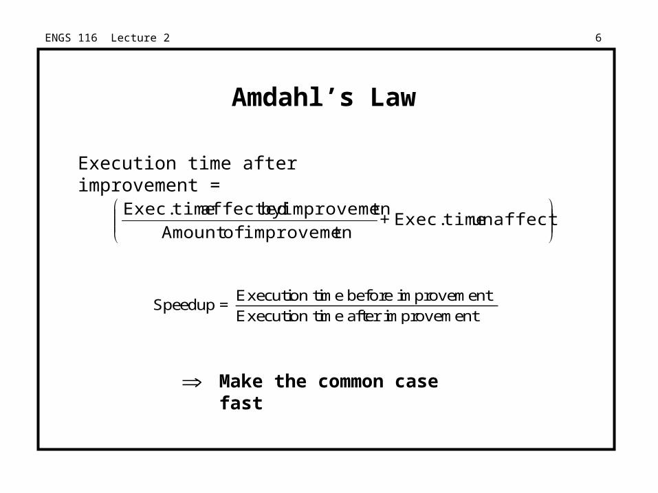
Amdahl’s Law
Execution time after improvement =
unaffected timeExec.
timprovemen ofAmount
timprovemenby affected timeExec.+
Speedup = Execution time before improvementExecution time after improvement
Make the common case fast
ENGS 116 Lecture 2 7
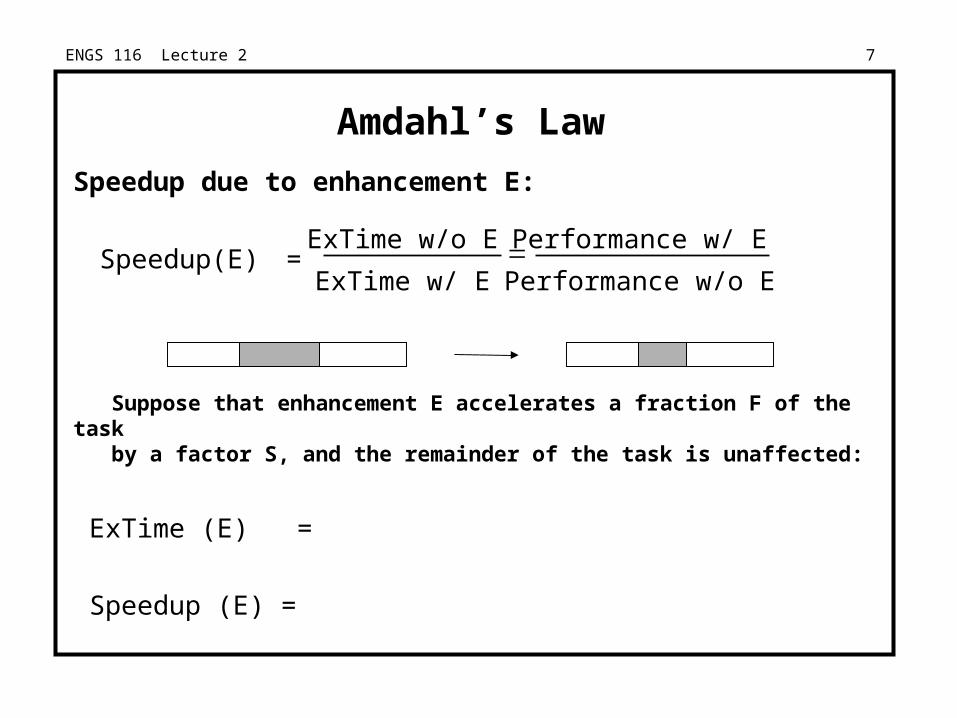
Speedup due to enhancement E:
Suppose that enhancement E accelerates a fraction F of the task by a factor S, and the remainder of the task is unaffected:
ExTime (E) =
Speedup (E) =
Amdahl’s Law
Speedup(E) = ExTime w/o E
ExTime w/ E Performance w/ E
Performance w/o E
ENGS 116 Lecture 2 8
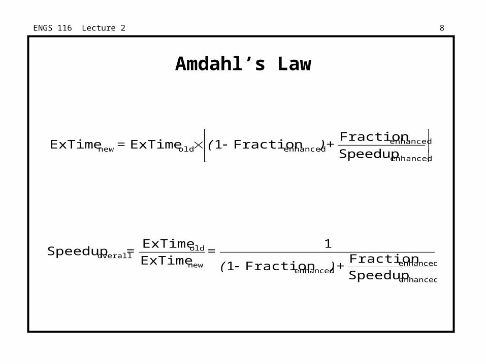
Amdahl’s Law
enhanced
enhancedenhancedoldnew Speedup
FractionFraction1ExTimeExTime +)(=
enhanced
enhancedenhanced
new
old overall
SpeedupFraction
Fraction1
1
ExTime
ExTimeSpeedup
+)(==
ENGS 116 Lecture 2 9
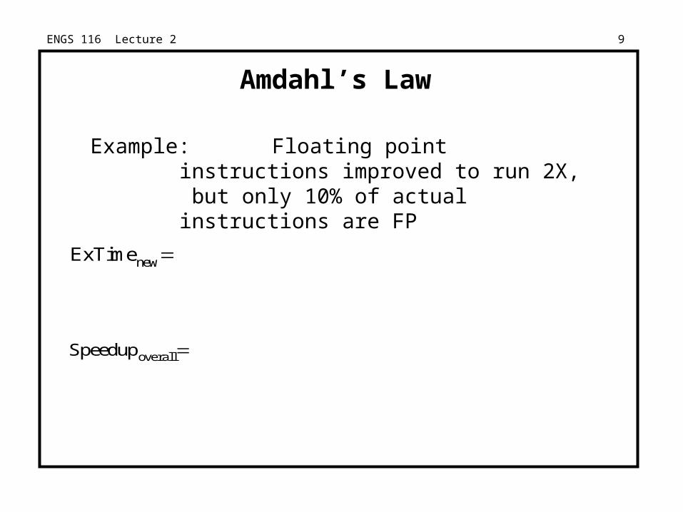
Amdahl’s Law
Example: Floating point instructions improved to run 2X, but only 10% of actual instructions are FP
ExTimenew=
Speedupoverall=
ENGS 116 Lecture 2 10
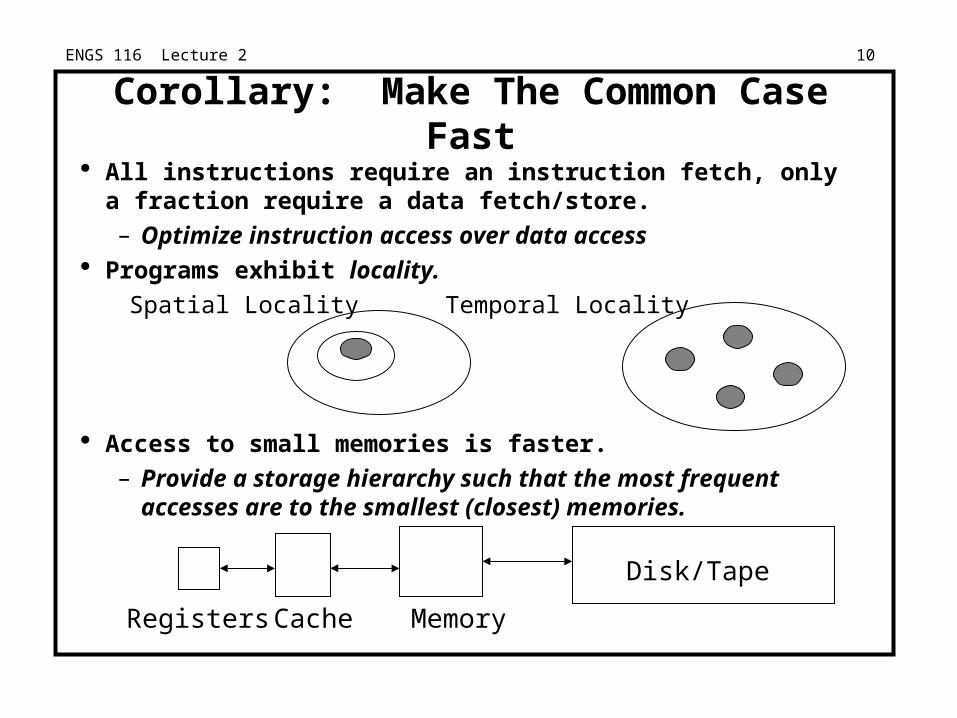
Corollary: Make The Common Case Fast All instructions require an instruction fetch, only a fraction require a
data fetch/store.
– Optimize instruction access over data access Programs exhibit locality.
Spatial Locality Temporal Locality
Access to small memories is faster.
– Provide a storage hierarchy such that the most frequent accesses are to the smallest (closest) memories.
Disk/Tape
Memory CacheRegisters
ENGS 116 Lecture 2 11
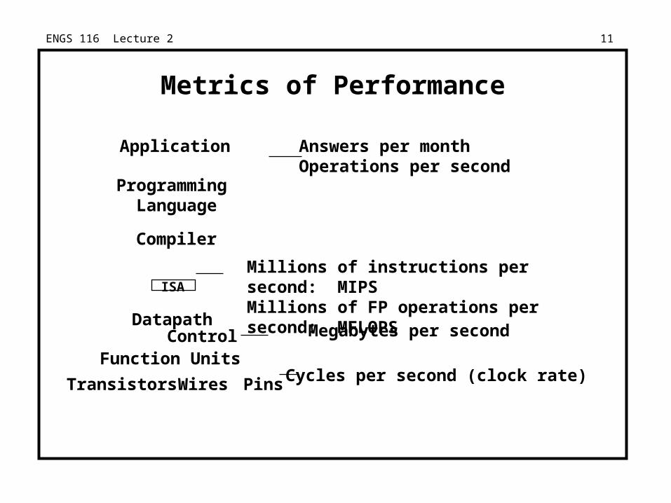
Metrics of Performance
Compiler
Programming Language
Application
DatapathControl
Transistors Wires Pins
ISA
Function Units
Millions of instructions per second: MIPSMillions of FP operations per second: MFLOPS
Cycles per second (clock rate)
Megabytes per second
Answers per monthOperations per second
ENGS 116 Lecture 2 12
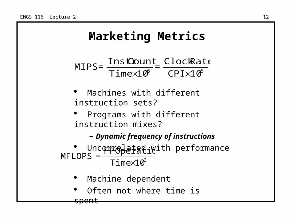
Marketing Metrics
Machines with different instruction sets? Programs with different instruction mixes?
– Dynamic frequency of instructions
Uncorrelated with performance
66 10CPI
RateClock
10Time
CountInstr MIPS
==
610Time
Operations FPMFLOPS
=
Machine dependent Often not where time is spent
ENGS 116 Lecture 2 13
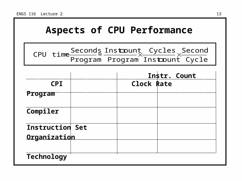
Aspects of CPU Performance
Instr. Count CPI Clock Rate
Program
Compiler
Instruction Set
Organization
Technology
Cycle
Seconds
countInstr
Cycles
Program
countInstr =
Program
Seconds = timeCPU
ENGS 116 Lecture 2 14
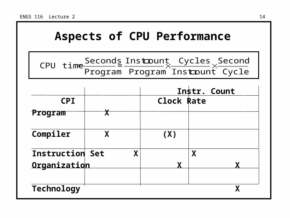
Aspects of CPU Performance
Instr. Count CPI Clock Rate
Program X
Compiler X (X)
Instruction Set X X
Organization X X
Technology X
Cycle
Seconds
countInstr
Cycles
Program
countInstr =
Program
Seconds = timeCPU
ENGS 116 Lecture 2 15
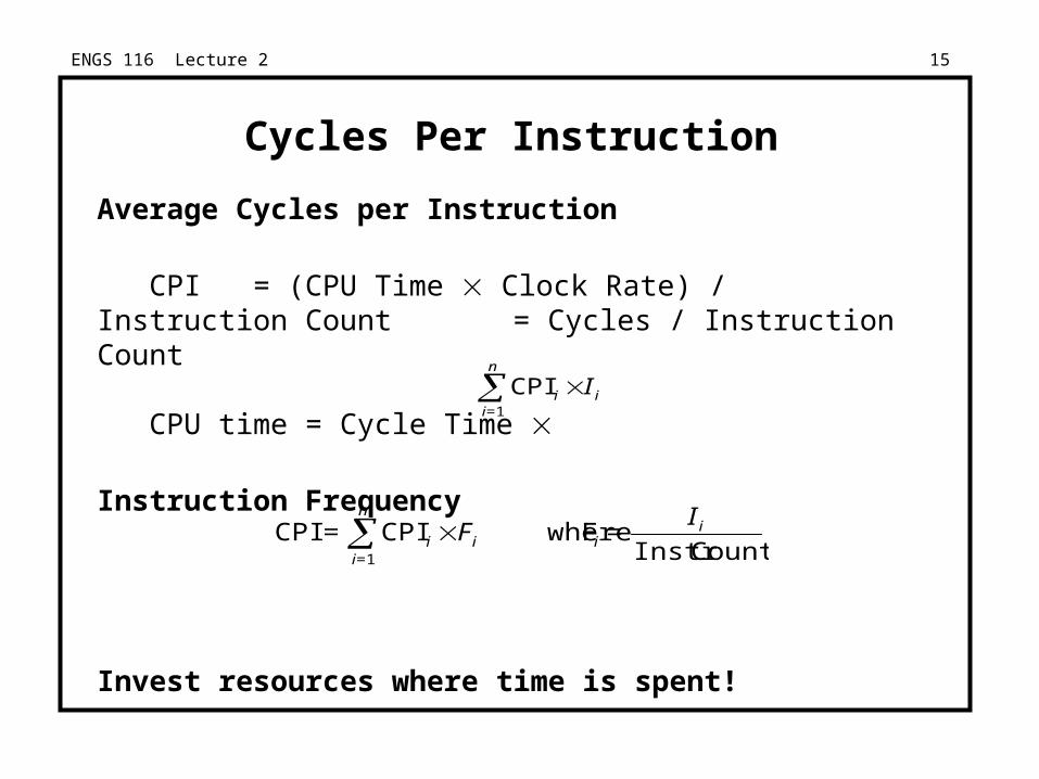
Average Cycles per Instruction
CPI = (CPU Time Clock Rate) / Instruction Count = Cycles / Instruction Count
CPU time = Cycle Time
Instruction Frequency
Invest resources where time is spent!
Cycles Per Instruction
n
=iii I
1
CPI
CountInstr F whereCPICPI
1
iii
n
=ii
I=F=
ENGS 116 Lecture 2 16
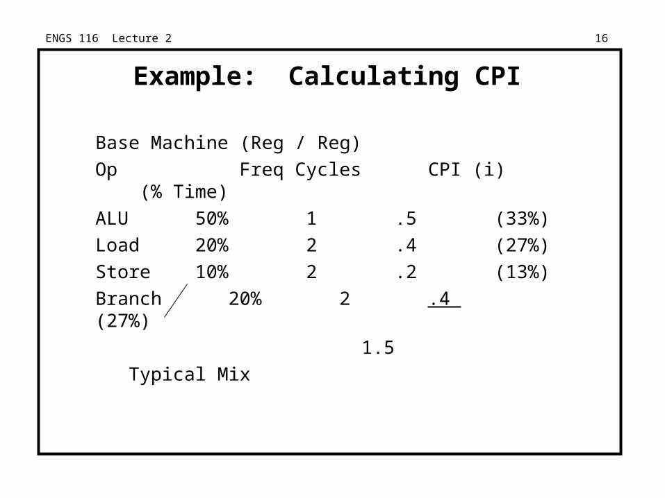
Example: Calculating CPI
Base Machine (Reg / Reg)
Op Freq Cycles CPI (i) (% Time)
ALU 50% 1 .5 (33%)
Load 20% 2 .4 (27%)
Store 10% 2 .2 (13%)
Branch 20% 2 .4 (27%)
1.5
Typical Mix
ENGS 116 Lecture 2 17
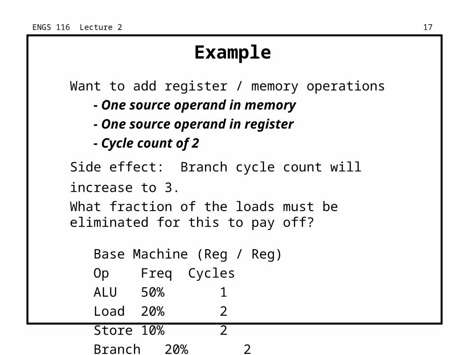
Example
Want to add register / memory operations
- One source operand in memory
- One source operand in register
- Cycle count of 2
Side effect: Branch cycle count will increase to 3.
What fraction of the loads must be eliminated for this to pay off?
Base Machine (Reg / Reg)
Op Freq Cycles
ALU 50% 1
Load 20% 2
Store 10% 2
Branch 20% 2
ENGS 116 Lecture 2 18
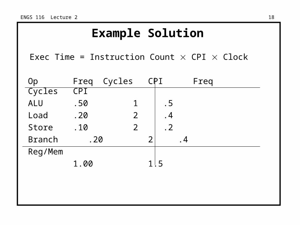
Example Solution
Exec Time = Instruction Count CPI Clock
Op Freq Cycles CPI Freq Cycles CPI
ALU .50 1 .5
Load .20 2 .4
Store .10 2 .2
Branch .20 2 .4
Reg/Mem
1.00 1.5
ENGS 116 Lecture 2 19
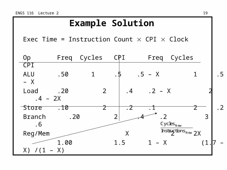
Example Solution
Exec Time = Instruction Count CPI Clock
Op Freq Cycles CPI Freq Cycles CPI
ALU .50 1 .5 .5 – X 1 .5 – X
Load .20 2 .4 .2 – X 2 .4 – 2X
Store .10 2 .2 .1 2 .2
Branch .20 2 .4 .2 3 .6
Reg/Mem X 2 2X
1.00 1.5 1 – X (1.7 – X) /(1 – X)
CPINew must be normalized to new instruction frequency
Cycles New
Instructions New
ENGS 116 Lecture 2 20
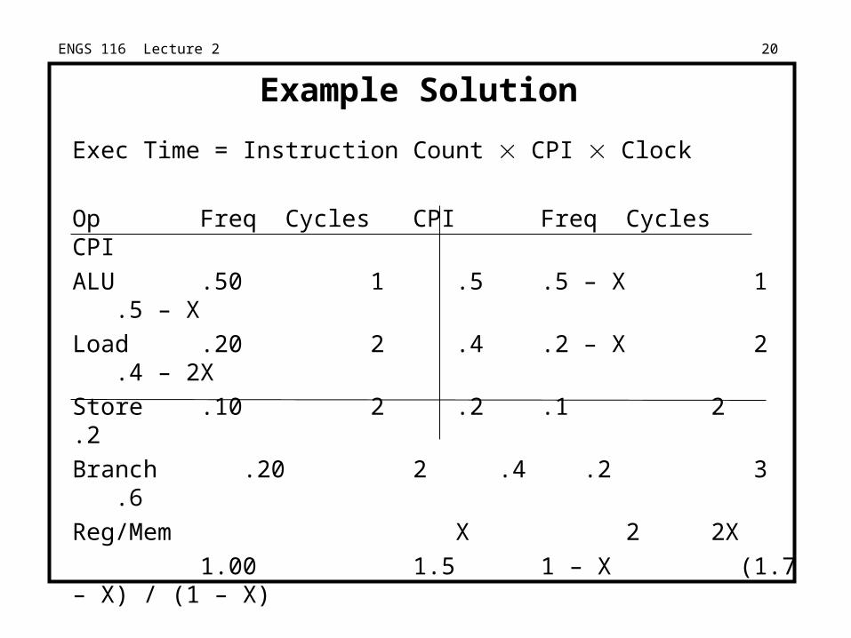
Example Solution
Exec Time = Instruction Count CPI Clock
Op Freq Cycles CPI Freq Cycles CPI
ALU .50 1 .5 .5 – X 1 .5 – X
Load .20 2 .4 .2 – X 2 .4 – 2X
Store .10 2 .2 .1 2 .2
Branch .20 2 .4 .2 3 .6
Reg/Mem X 2 2X
1.00 1.5 1 – X (1.7 – X) / (1 – X)
Instr CntOld CPIOld ClockOld = Instr CntNew CPINew ClockNew
ENGS 116 Lecture 2 21
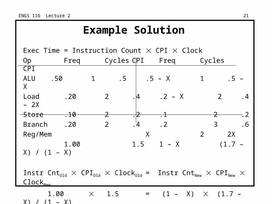
Example Solution
Exec Time = Instruction Count CPI Clock
Op Freq Cycles CPI Freq Cycles CPI
ALU .50 1 .5 .5 – X 1 .5 – X
Load .20 2 .4 .2 – X 2 .4 – 2X
Store .10 2 .2 .1 2 .2
Branch .20 2 .4 .2 3 .6
Reg/Mem X 2 2X
1.00 1.5 1 – X (1.7 – X) / (1 – X)
Instr CntOld CPIOld ClockOld = Instr CntNew CPINew ClockNew
1.00 1.5 = (1 – X) (1.7 – X) / (1 – X)
1.5 = 1.7 – X
0.2 = X
ALL loads must be eliminated for this to be a win!