ENGR 205 Project Report Mariraja.P

1

Car design performance optimization by interpolation

ENGR 205 Individual Project Report

By Mariraja.P,

Department of Mechanical Engineering

California State University, Fresno, CA

Dr. Fayzul Pasha

Department of Civil and Geomatics Engineering

California State University, Fresno, CA

2

Contents

No. Title Page No.

1. Summary 5

2. Introduction 5

3. Data 6

4. Formulas for calculation 7

5. Methodology 8

6. Results and discussions 10

7. Analysis 23

8. Appendices 23

8. Conclusion 26

9. References 27

3

Tables

No. Title Page No.

1. Car specifications 7

2. Tractive Force and Velocity 10

3. Total Resistance (Rt) and Acceleration (A) 12

4, 6, 8, 10 Linear Interpolation Points 14,15,16,17

5, 7, 9, 11 Newton’s Interpolating Points 14,15,16,17

12 Linear Spline Interpolation Points 19

13 Quadratic Spline coefficients values 21

14 Quadratic Spline Interpolation Points 22

4

Table of Diagrams

No. Title Page No.

1. Vehicle Design Data of BMW 740li – Petrol variant 6

2. Force Vs Velocity 11

3. Velocity vs Acceleration 13

4. Engine Speed Vs Torque 13

5. Engine Speed Vs Brake power 14

6. Linear and Newton’s Interpolation for Velocity Vs Force 15

7. Linear and Newton’s Interpolation for Velocity Vs Acceleration 16

8. Linear and Newton’s Interpolation for Engine Speed Vs Torque 17

9. Linear and Newton’s Interpolation for Engine Speed Vs Brake Power 18

10. Linear Splines for Engine Speed Vs Brake Power 19

11. Quadratic Splines for Engine Speed Vs Brake Power 22

5

Summary

The aim of the project is to consider design criteria of a car and optimize the performanceby interpolating the values to predict the various performance parameters of the car. The enginespecifications, transmission gear ratios, chassis dimensions, wheel descriptions are taken up forformulating brake power, equivalent torque, tractive force, velocity and acceleration of vehicle.Air resistance, rolling resistance are used to calculate the total resistance.

Introduction

The effect on the performance due to the design of the car is being studied. Thedimensions from the design are used to calculate the frontal area which determines the airresistance. The gear ratios and the weight of the car are used for calculating the force of the car.Using force value velocity and acceleration are calculated. Transmission efficiency is assumed tobe 85%. Transmission efficiency is the efficiency put together of all the components thatconnects the engine with the wheels. In this case the rear wheels.

The internal combustion engine (ICE) is an engine in which the combustion of a fuel(normally a fossil fuel) occurs in a combustion chamber that is an integral part of the workingfluid flow circuit. From the spark ignition data the output torque value is obtained. Brake powerand torque values are calculated which determine the acceleration of the car. Brake power is theoutput power from the internal combustion engine. Torque is the tendency to rotate an about anaxis. The resistance offered by the car is by the rolling resistance and air resistance. The rollingresistance caused by the weight of the car increases upon the increase of velocity. The frontalarea leads to air resistance. These resistance along with the transmission efficiency determine theacceleration of the car.

Through these calculation the cars performance can be significantly improved by makingchanges in the design of the car, decreasing the weight and frontal area, reducing thetransmission losses, altering the gear ratios for a more flat torque curve. Having a flat torqueensures a good acceleration and mileage for the car. It is also ensured that the entitled customerneeds are met at the same time.

Using interpolation intermediate values are predicted which shows the performance ofthe car. Linear interpolation and Newton’s interpolating polynomial is used to find unknownvalue. This helps in the study of the behavior of the car. This can also be used as an optimizationtechnique to alter the response the car provides.

As an example BMW 740li petrol variant is used. The matlab coding would be able topredict the unknown value, which can be used to predict the performance of the vehicle. This canbe used to optimize the performance for particular predicted values. The code has been createdfor newton’s interpolating polynomial function.

6

The weight of a car influences fuel consumption and performance, with more weightresulting in increased fuel consumption and decreased performance. Most automobiles in usetoday are propelled by an internal combustion engine, fueled by deflagration of gasoline (alsoknown as petrol) or diesel.

Data

The various dimensions of the car in mm are taken. These determine the weight of the carand also the aerodynamic drag of the car. The drag increases with the increase in the velocity andacceleration.

Fig. 1. Vehicle Design Data of BMW 740li – Petrol variant

The BMW 7 Series is a line of full-size luxury vehicles produced by the Germanautomaker BMW. Introduced in 1977, it is BMW's flagship car and is only available as a sedanor extended-length limousine. The 7 Series traditionally introduces technologies and exteriordesign themes before they trickle down to smaller sedans in BMW's lineup.[1]

ENGINEDisplacement 2979ccStroke & bore 89.6 mm & 84.0 mmMax. Power 240kw @5800rpmMax. Torque 450 Nm @1500-4500 rpmTRANSMISSION Six speed automaticGear ratios I Gear 4.17

7

II Gear 2.34III Gear 1.52IV Gear 1.4V Gear 0.87VI Gear 0.69

Final drive ratio 3.73CHASSISLength 5072mmWidth 1902 mmHeight 1479mmGround clearance 144mmFrontal area 2.41m2

Gross weight limit 2475 kgKerb weight 1860 kg

Table. 1. Car specifications

Formulas for calculation [5]

The rated rpm is the rpm at which the vehicle is supposed to run at all times. Therefore rated rpmis taken into consideration for all calculation purposes.

Nmin= 800 to 1000 rpm

Nmax= 1.1 Nrated (1.0)

Nrated = 6380 rpm

Brake power is the power output of the drive shaft of an engine without the power loss caused bygears, transmission, friction, etc. It's called also pure power, useful power, true power or wheelpower as well as other terms.[2]

B.P. = B.P.rated

2

1ratedratedrated NN

NN

NN kW (2.0)

Equivalent torque is the torque that is obtained at particular brake power to the rpm.

Equivalent torque (Te) =N

BP26000 Nm (3.0)

Force (F) =rGT Te N (4.0)

Velocity (V) =65.2

GrN (5.0)

8

Air Resistance

This is due to the frontal area of the car. Improving aerodynamics can reduce this effect.In aerodynamics, aerodynamic drag is the fluid drag force that acts on any moving solid body inthe direction of the fluid free stream flow. From the body's perspective (near-field approach), thedrag comes from forces due to pressure distributions over the body surface and forces due to skinfriction, which is a result of viscosity. The drag force comes from three natural phenomena:shock waves, vortex sheet, and viscosity. [4]

Ra = KaAV2 (6.0)

Rolling Resistance

Resistance due to the friction caused by the tires on the road because of the weight of thecar. Rolling resistance decreases with velocity. Rolling resistance, sometimes called rollingfriction or rolling drag, is the force resisting the motion when a body (such as a ball, tire, orwheel) rolls on a surface. It is mainly caused by non-elastic effects; that is, not all the energyneeded for deformation (or movement) of the wheel, roadbed, etc. is recovered when thepressure is removed. Another cause of rolling resistance lies in the slippage between the wheeland the surface, which dissipates energy. In analogy with sliding friction, rolling resistance isoften expressed as a coefficient times the normal force. [4]

Rr = (0.015+0.00016V) W (7.0)

Total Resistance

It represents the sum of the rolling resistance and air resistance.

Rt = Ra+Rr (8.0)

We= (1.04 + 0.0025 G2) W (9.0)

A =e

T

WRFg )( (10.0)

Methodology

Linear interpolation, Newton’s Interpolating polynomial and Splines are used to estimatethe value of the unknown point. These methods are for fitting a curve to the unknown point.

Linear Interpolation

The simplest form of interpolation is to connect two data points with a straight line. Thenotation f1(x) designates that this is a first order interpolating polynomial. Besides representing

9

the slope of the line connecting the points, the term [f(x1) – f(x0)]/(x1 – x0) is a finite divideddifference.approximation of the first derivative. For better approximation smaller intervalbetween data points are to be taken. A continuous function will be better approximated by astraight line. ( ) = ( ) + ( ) ( ) ( − ) (11.0)

General form of Newton’s Interpolating Polynomial

Newton's formula is of interest because it is the straightforward and natural differences-version of Taylor's polynomial. Taylor's polynomial tells where a function will go, based on its yvalue, and its derivatives (its rate of change, and the rate of change of its rate of change, etc.) atone particular x value. Newton's formula is Taylor's polynomial based on finite differencesinstead of instantaneous rates of change. With the Newton form of the interpolating polynomial acompact and effective algorithm exists for combining the terms to find the coefficients of thepolynomial.[3]

For any given finite set of data points, there is only one polynomial, of least possibledegree, that passes through all of them. To fit nth-order polynomial n + 1 data points areconsidered. The nth-order polynomial is [6]( ) = + ( − ) + ⋯+ ( − )( − )… ( − ) (12.0)

Data points can be used to evaluate the coefficients b0, b1,…, bn. Data points are used to evaluatethe coefficients:

b0 = f (x0)

b1 = f [x1, x0]

b2 = f [x2, x1, x0]

.

.

bn = f [xn, xn-1,…., x1, x0]

For nth divided difference

[ , , … , , ] = [ , ,…, ] [ , ,..., ] (13.0)

10

Results and discussion

Using the equations 1 to 10 and the values from the Table. 1. Car specifications,Tractive force (F), Velocity (V), Total Resistance (Rt) and Acceleration (A) are calculated.

Table. 2. Tractive force and Velocity

NBP

TeI

IIIII

IVV

VII

IIIII

IVV

VI220

.0000

9.4357

409.77

07153

53.407

2861

5.5810

5596.4

458515

4.6211

3203.2

288254

0.4918

1.8834

3.3562

5.1668

5.6097

9.0271

11.382

0440

.0000

19.483

3423

.0601

15851.

3374

8894.9

951577

7.9455

5321.7

919330

7.1136

2622.8

8323.7

6676.7

12510.

3337

11.219

418.

0542

22.764

0880

.0000

41.100

4446

.2260

16719.

3248

9382.0

671609

4.3342

5613.2

026348

8.2044

2766.5

0707.5

33413.

4249

20.667

322.

4388

36.108

445.

5280

1100.0

00052.

5126

456.10

26170

89.381

9958

9.7251

6229.2

231573

7.4424

3565.4

106282

7.7394

9.4168

16.781

225.

8342

28.048

545.

1355

56.910

0132

0.0000

64.222

5464

.8415

17416.

8146

9773.4

643634

8.5751

5847.3

718363

3.7239

2881.9

19011.

3001

20.137

431.

0010

33.658

254.

1627

68.292

0154

0.0000

76.151

5472

.4428

17701.

6230

9933.2

848645

2.3901

5942.9

909369

3.1444

2929.0

45513.

1835

23.493

636.

1678

39.267

963.

1898

79.674

0176

0.0000

88.221

0478

.9065

17943.

80691

0069.1

866654

0.6682

6024.2

997374

3.6720

2969.1

19115.

0668

26.849

941.

3347

44.877

672.

2169

91.056

1198

0.0000

100.35

24484

.2326

18143.

36651

0181.1

697661

3.4094

6091.2

981378

5.3067

3002.1

39816.

9502

30.206

146.

5015

50.487

381.

2440

102.43

81220

0.0000

112.46

71488

.4211

18300.

30181

0269.2

341667

0.6136

6143.9

862381

8.0486

3028.1

07518.

8335

33.562

351.

6683

56.097

090.

2711

113.82

01242

0.0000

124.48

66491

.4720

18414.

61261

0333.3

797671

2.2808

6182.3

639384

1.8976

3047.0

22220.

7169

36.918

656.

8352

61.706

799.

2982

125.20

21264

0.0000

136.33

22493

.3852

18486.

29901

0373.6

067673

8.4112

6206.4

313385

6.8538

3058.8

84022.

6002

40.274

862.

0020

67.316

4108

.3253

136.58

41286

0.0000

147.92

54494

.1609

18515.

36111

0389.9

149674

9.0045

6216.1

884386

2.9171

3063.6

92824.

4836

43.631

067.

1688

72.926

1117

.3524

147.96

61308

0.0000

159.18

76493

.7989

18501.

79881

0382.3

044674

4.0610

6211.6

351386

0.0875

3061.4

48726.

3670

46.987

372.

3357

78.535

8126

.3795

159.34

81330

0.0000

170.04

02492

.2993

18445.

61211

0350.7

752672

3.5804

6192.7

715384

8.3651

3052.1

51628.

2503

50.343

577.

5025

84.145

6135

.4066

170.73

01352

0.0000

180.40

46489

.6621

18346.

80111

0295.3

272668

7.5630

6159.5

975382

7.7499

3035.8

01630.

1337

53.699

782.

6693

89.755

3144

.4337

182.11

21374

0.0000

190.20

22485

.8873

18205.

36561

0215.9

606663

6.0086

6112.1

132379

8.2418

3012.3

98632.

0170

57.056

087.

8361

95.365

0153

.4609

193.49

41396

0.0000

199.35

45480

.9749

18021.

30581

0112.6

752656

8.9172

6050.3

185375

9.8408

2981.9

42733.

9004

60.412

293.

0030

100.97

47162

.4880

204.87

61418

0.0000

207.78

28474

.9249

17794.

6216

9985.4

711648

6.2889

5974.2

135371

2.5470

2944.4

33835.

7837

63.768

498.

1698

106.58

44171

.5151

216.25

81440

0.0000

215.40

86467

.7372

17525.

3130

9834.3

483638

8.1237

5883.7

981365

6.3603

2899.8

71937.

6671

67.124

7103

.3366

112.19

41180

.5422

227.64

01462

0.0000

222.15

33459

.4120

17213.

3801

9659.3

068627

4.4215

5779.0

724359

1.2807

2848.2

57139.

5504

70.480

9108

.5035

117.80

38189

.5693

239.02

21484

0.0000

227.93

82449

.9491

16858.

8227

9460.3

466614

5.1824

5660.0

364351

7.3083

2789.5

89441.

4338

73.837

1113

.6703

123.41

35198

.5964

250.40

42506

0.0000

232.68

49439

.3486

16461.

6410

9237.4

676600

0.4063

5526.6

900343

4.4431

2723.8

68743.

3171

77.193

4118

.8371

129.02

32207

.6235

261.78

62528

0.0000

236.31

47427

.6105

16021.

8349

8990.6

700584

0.0933

5379.0

333334

2.6850

2651.0

95045.

2005

80.549

6124

.0040

134.63

29216

.6506

273.16

82550

0.0000

238.74

90414

.7348

15539.

4044

8719.9

536566

4.2433

5217.0

662324

2.0340

2571.2

68447.

0838

83.905

8129

.1708

140.24

26225

.6777

284.55

02572

0.0000

239.90

93400

.7215

15014.

3496

8425.3

185547

2.8564

5040.7

888313

2.4902

2484.3

88848.

9672

87.262

1134

.3376

145.85

23234

.7048

295.93

22594

0.0000

239.71

70385

.5706

14446.

6704

8106.7

647526

5.9326

4850.2

011301

4.0535

2390.4

56250.

8505

90.618

3139

.5045

151.46

20243

.7319

307.31

42616

0.0000

238.09

34369

.2821

13836.

3667

7764.2

921504

3.4718

4645.3

030288

6.7240

2289.4

70852.

7339

93.974

5144

.6713

157.07

17252

.7591

318.69

62638

0.0000

234.96

00351

.8559

13183.

4387

7397.9

009480

5.4741

4426.0

945275

0.5016

2181.4

32354.

6173

97.330

8149

.8381

162.68

14261

.7862

330.07

82

Tractiv

e Force

(F)Vel

ocity (V

)

11

Fig. 2. Velocity Vs Force

The Fig. 2. shows the velocity produced at every gear because of the force which results due tothe torque produced by the engine which in turn is a result of the brake horse power generated bythe Internal combustion engine. The following Table. 3. represents the acceleration of the vehicleafter considering the resistance that is caused due to air and rolling of the vehicle.

0.0000

2000.0000

4000.0000

6000.0000

8000.0000

10000.0000

12000.0000

14000.0000

16000.0000

18000.0000

20000.0000

0.0000 50.0000 100.0000 150.0000 200.0000 250.0000 300.0000 350.0000

Forc

e

Velocity

I gear

II gear

III gear

IV gear

V gear

VI gear

12

Table. 3. Total Resistance (Rt) and Acceleration (A)

III

IIIIV

VVI

III

IIIIV

VVI

0.265

00.8

416

1.994

52.3

510

6.088

09.6

787

37.00

4649

.4536

54.32

2054

.9425

57.07

3657

.5992

1.060

03.3

662

7.977

99.4

041

24.35

2138

.7147

38.20

2851

.0549

56.08

1056

.7215

58.92

1659

.4642

4.240

013

.4649

31.91

1537

.6165

97.40

8315

4.859

040

.2872

53.84

0559

.1408

59.81

6362

.1364

62.70

876.6

249

21.03

8949

.8617

58.77

5815

2.200

524

1.967

241

.1734

55.02

4860

.4417

61.13

2063

.5032

64.08

809.5

399

30.29

6071

.8009

84.63

7221

9.168

734

8.432

741

.9555

56.07

0161

.5899

62.29

3364

.7096

65.30

5512

.9849

41.23

6297

.7290

115.2

006

298.3

130

474.2

557

42.63

3756

.9764

62.58

5463

.3002

65.75

5566

.3611

16.95

9953

.8596

127.6

461

150.4

661

389.6

333

619.4

360

43.20

7857

.7437

63.42

8264

.1527

66.64

1067

.2547

21.46

4868

.1660

161.5

520

190.4

336

493.1

297

783.9

736

43.67

8058

.3719

64.11

8464

.8507

67.36

6167

.9865

26.49

9884

.1556

199.4

470

235.1

032

608.8

021

967.8

687

44.04

4158

.8612

64.65

5865

.3943

67.93

0868

.5564

32.06

4810

1.828

224

1.330

828

4.474

973

6.650

511

71.12

1144

.3062

59.21

1565

.0406

65.78

3468

.3351

68.96

4338

.1597

121.1

840

287.2

036

338.5

486

876.6

750

1393

.7309

44.46

4359

.4228

65.27

2666

.0182

68.57

8969

.2104

44.78

4714

2.222

933

7.065

439

7.324

410

28.87

5516

35.69

8144

.5183

59.49

5165

.3520

66.09

8568

.6623

69.29

4651

.9396

164.9

449

390.9

161

460.8

023

1193

.2520

1897

.0226

44.46

8459

.4283

65.27

8766

.0243

68.58

5369

.2169

59.62

4518

9.350

144

8.755

752

8.982

213

69.80

4621

77.70

4644

.3145

59.22

2665

.0527

65.79

5768

.3478

68.97

7267

.8395

215.4

383

510.5

842

601.8

642

1558

.5333

2477

.7438

44.05

6558

.8778

64.67

4165

.4127

67.95

0068

.5757

76.58

4424

3.209

657

6.401

767

9.448

317

59.43

8027

97.14

0543

.6945

58.39

4164

.1427

64.87

5367

.3917

68.01

2385

.8593

272.6

641

646.2

082

761.7

344

1972

.5187

3135

.8946

43.22

8657

.7714

63.45

8764

.1834

66.67

3067

.2870

95.66

4330

3.801

672

0.003

684

8.722

621

97.77

5534

94.00

6042

.6586

57.00

9662

.6219

63.33

7265

.7939

66.39

9810

5.999

233

6.622

379

7.787

994

0.412

824

35.20

8338

71.47

4841

.9846

56.10

8961

.6325

62.33

6464

.7543

65.35

0711

6.864

137

1.126

187

9.561

110

36.80

5126

84.81

7142

68.30

0941

.2065

55.06

9160

.4904

61.18

1363

.5544

64.13

9612

8.259

040

7.313

096

5.323

311

37.89

9529

46.60

2046

84.48

4540

.3245

53.89

0359

.1956

59.87

1762

.1940

62.76

6714

0.183

944

5.183

010

55.07

4512

43.69

6032

20.56

2951

20.02

5439

.3385

52.57

2657

.7481

58.40

7760

.6732

61.23

1915

2.638

848

4.736

111

48.81

4613

54.19

4535

06.69

9955

74.92

3738

.2484

51.11

5856

.1479

56.78

9258

.9920

59.53

5216

5.623

752

5.972

412

46.54

3614

69.39

5038

05.01

2960

49.17

9337

.0544

49.52

0154

.3950

55.01

6357

.1503

57.67

6617

9.138

656

8.891

713

48.26

1515

89.29

7741

15.50

2065

42.79

2435

.7563

47.78

5352

.4895

53.08

9055

.1482

55.65

6119

3.183

561

3.494

214

53.96

8417

13.90

2444

38.16

7170

55.76

2834

.3542

45.91

1550

.4313

51.00

7352

.9857

53.47

3720

7.758

465

9.779

715

63.66

4318

43.20

9147

73.00

8275

88.09

0532

.8481

43.89

8748

.2203

48.77

1150

.6628

51.12

9422

2.863

370

7.748

416

77.34

9019

77.21

8051

20.02

5481

39.77

5731

.2380

41.74

6945

.8567

46.38

0548

.1795

48.62

32

Tota

l Res

istan

ce (R

t)Ac

celer

ation

(A)

13

Fig. 3. Velocity Vs Acceleration

Fig. 4. Engine Speed Vs Torque

0.0000

10.0000

20.0000

30.0000

40.0000

50.0000

60.0000

70.0000

80.0000

0.0000 50.0000 100.0000 150.0000 200.0000 250.0000 300.0000 350.0000

Acce

lera

tion

Velocity

I gear

II gear

III gear

IV gear

V gear

VI gear

0.0000

100.0000

200.0000

300.0000

400.0000

500.0000

600.0000

0 1000 2000 3000 4000 5000 6000 7000

Torq

ue

Engine Speed

Torque

14

Fig. 5. Engine Speed Vs Brake power

Interpolation for Velocity and Force

x0 1.8834 f(x0) 15353.4072x1 54.6173 f(x1) 13183.4387x 30.1337 f(x) 14190.9242

Table. 4. Linear Interpolation Points

b0 15353.4072b1 105.9419b2 0.0207

x 31f2(x) 18438.5988

Table. 5. Newton’s Interpolating Points

0.0000

50.0000

100.0000

150.0000

200.0000

250.0000

300.0000

0 1000 2000 3000 4000 5000 6000 7000

Brak

e Po

wer

Engine Speed

Brake Power

x0 1.8834 f(x0) 15353.4072x1 30.1337 f(x1) 18346.2990x2 54.6173 f(x2) 13183.4387

15

Fig. 6. Linear and Newton’s Interpolation for Velocity Vs Force

Interpolation for Velocity and Acceleration

x0 1.8834 f(x0) 37.0046x1 54.6173 f(x1) 31.2380x 43.2286 f(x) 32.48336918


x0 1.8834 f(x0) 37.0046 b0 37.0046x1 30.1337 f(x1) 44.0565 b1 0.249622x2 54.6173 f(x2) 31.2380 b2 -0.0439x 31

f2(x) 43.1655

0.0000

2000.0000

4000.0000

6000.0000

8000.0000

10000.0000

12000.0000

14000.0000

16000.0000

18000.0000

20000.0000

0 10 20 30 40 50 60

Forc

e

Velocity

Linear

Newton’s InterpolatingPolynomial


16

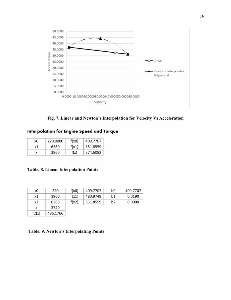
Fig. 7. Linear and Newton’s Interpolation for Velocity Vs Acceleration

Interpolation for Engine Speed and Torque

x0 220.0000 f(x0) 409.7707x1 6380 f(x1) 351.8559x 3960 f(x) 374.6082


x0 220 f(x0) 409.7707 b0 409.7707x1 3960 f(x1) 480.9749 b1 0.0190x2 6380 f(x2) 351.8559 b2 0.0000x 3740

f2(x) 486.1766

0.0000

5.0000

10.0000

15.0000

20.0000

25.0000

30.0000

35.0000

40.0000

45.0000

50.0000

0.0000 10.000020.000030.000040.000050.000060.0000

Acce

lera

tion

Velocity

Linear

Newton's InterpolationPolynomial


17

Fig. 8. Linear and Newton’s Interpolation for Engine Speed Vs Torque

Interpolation for Engine Speed and Brake Power

x0 220 f(x0) 9.4357x1 6380 f(x1) 234.9600x 3960 f(x) 146.3611


x0 220 f(x0) 9.4357x1 3960 f(x1) 199.3545x2 6380 f(x2) 234.9600b0 9.4357b1 0.0508b2 0.0000x 4180

f2(x) 205.5938

0.0000

100.0000

200.0000

300.0000

400.0000

500.0000

600.0000

0.0000 1000.0000 2000.0000 3000.0000 4000.0000 5000.0000 6000.0000 7000.0000

Torq

ue

Engine Speed


Newtons's Interpolation


18

Fig. 9. Linear and Newton’s Interpolation for Engine Speed Vs Brake Power

Linear Splines

With the help of mat lab code it is identified that the second order polynomials do notcapture the curvature between the data points of range 4000 to 7000 with respect to EngineSpeed. We therefore involve Linear Splines to interpolate and predict those values. Thefollowing equations are for the first-order splines.( ) = ( ) + ( − ) ≤ ≤ (14.0)( ) = ( ) + ( − ) ≤ ≤ (15.0)

.

.( ) = ( ) + ( − ) ≤ ≤ (16.0)

Where mi is the slope and is given as,= ( ) ( ) (17.0)

0.0000

50.0000

100.0000

150.0000

200.0000

250.0000

0 1000 2000 3000 4000 5000 6000 7000

Brak

e Po

wer

Engine Speed


Newton's Interpolating Polynomial

19

x f(x) Slope m4180 207.7828 7.2444994400 215.4086 6.4234954620 222.1533 5.5220124840 227.9382 4.5402975060 232.6849 3.4785555280 236.3147 2.336965500 238.749 1.1156575720 239.9093 -0.185235940 239.717 -1.565596160 238.0934 -3.025346380 234.96

x 5280f(x) 997.9671

Table. 12. Linear Spline Interpolation Points

Fig. 10. Linear Splines for Engine Speed Vs Brake Power

Quadratic Splines

Although Linear Splines could capture some curvature, Quadratic splines was able tocapture more curvature and result in an better prediction of the curve. For the n+1 = 11 pointsconsidered there are n=10 intervals. This implies there are 3n = 30 Unknowns. The 29 constantshave been solved using the four conditions of Quadratic splines method. Quadratic method hasfour conditions which are as follows,

200

210

220

230

240

250

0 1000 2000 3000 4000 5000 6000 7000

Brak

e Po

wer

Engine Speed

Linear Splines

20

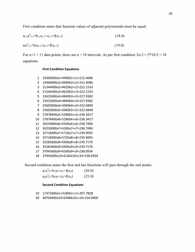
First condition states that function values of adjacent polynomials must be equal.

ai-1x2i-1+bi-1xi-1+ci-1=f(xi-1) (18.0)

aix2i-1+bixi-1+ci-1=f(xi-1) (19.0)

For n+1 = 11 data points, there are n = 10 intervals. As per first condition 2n-2 = 2*10-2 = 18equations.

First Condition Equations

1 19360000a1+4400b1+c1=215.40862 19360000a2+4400b2+c2=215.40863 21344400a2+4620b2+c2=222.15334 21344400a3+4620b3+c3=222.15335 23425600a3+4840b3+c3=227.93826 23425600a4+4840b4+c4=227.93827 25603600a4+5060b4+c4=232.68498 25603600a5+5060b5+c5=232.68499 27878400a5+5280b5+c5=236.3417

10 27878400a6+5280b6+c6=236.341711 30250000a6+5500a6+c6=238.749012 30250000a7+5500a7+c7=238.749013 32718400a7+5720a7+c7=239.909314 32718400a8+5720a8+c8=239.909315 35283600a8+5940a8+c8=239.717016 35283600a9+5940a9+c9=239.717017 37945600a9+6160a9+c9=238.093418 37945600a10+6160a10+c10=238.0934

Second condition states the first and last functions will pass through the end points.a1x20+b1x0+c1=f(x0) (20.0)anx2n+bnxn+cn=f(xn) (21.0)

Second Condition Equations

19 17472400a1+4180b1+c1=207.782820 40704400a10+6380b10+c10=234.9600

21

Third Condition21 8800a1+b1=8800a2+b222 9240a2+b2=9240a3+b323 9680a3+b3=9680a4+b424 10120a4+b4=10120a5+b525 10560a5+b5=10560a6+b626 11000a6+b6=11000a7+b727 11440a7+b7=11440a8+b828 11880a8+b8=11880a9+b929 12320a9+b9=12320a10+b10

Fourth Condition30 a1=0

b1 0.0347 b6 0.2602c1 62.8926 c6 -492.8935a2 0.0000 a7 0.0000b2 0.1949 b7 0.0349c2 -289.5474 c7 126.6065a3 0.0000 a8 0.0000b3 0.0417 b8 0.2942c3 64.3110 c8 -614.8303a4 0.0000 a9 0.0000b4 0.2178 b9 0.0443c4 -361.9962 c9 127.3646a5 0.0000 a10 0.0000b5 0.0445 b10 -0.0149c5 76.5977 c10 327.9301a6 0.0000

Table. 13. Quadratic Spline coefficients values

Third condition is that first derivatives at the interior knots must be equal

fi(x) = aix2+bix+ci (22.0)

f `(x)=2ax+b (23.0)

2ai-1xi-1+bi-1= 2aixi-1+bi (24.0)

22

The value of these constants are used to find the unknown function value between the 10intervals. There by optimization of the values is done.

x f(x)4180 207.7827974400 215.408586

x1 4300f(x1) 211.9423b1 0.0347c1 62.8926

Table. 14. Quadratic Spline Interpolation Points

Fig. 11. Quadratic Splines for Engine Speed Vs Brake Power

207.0000

208.0000

209.0000

210.0000

211.0000

212.0000

213.0000

214.0000

215.0000

216.0000

4150 4200 4250 4300 4350 4400 4450

Brak

e Po

wer

Engine Speed

Quadratic Interpolation

23

Analysis

In all the analysis graphs drawn it is observed that the Newton’s polynomial methodapproximates much better than the linear interpolation. The reason why the mat lab code wasbased on the Newton’s method. This implies that the Lagrange interpolation also yields the sameresult, as it is just the reformulation of the Newton’s method. Cubic splines are not useful asNewton’s method and Quadratic Splines could capture all the curvature required in the problem.

With the help of the mat lab code prediction for various parameters is possible. Let usconsider an example of how the predicted value affects the design. For gears III, IV, V, VI weare able to predict that acceleration values coincide for a particular range between 10 to 100(m/s), this can be used to further update the vaue of the gear ratio. There by we are directlyaltering the mechanical design of the component. Similarly we can alter the various designparameters of the car by altering the predicted values.

Appendices

Mat lab code

The code uses nested ‘for’ loop for calculating the Newton’s interpolating method topredict the value. The x and f(x) values for various gear values are given. Switch loop is used toselect the particular gear. Then for respective gear ratio the force and velocity values areselected. Then the code calculates coeffiecients b0,b1,…,bn. Then the interpolating methodformula is calculated and the resulting values are provided.

format long;k= input ('Enter the gear number between 1 to 6:');switch k

case 1x1= input('Enter a value between 2 and 50:');x= [0 1.8834 3.7667 7.5334 9.4168 11.3001 13.1835 15.0668 16.9502

18.8335 20.7169 22.6002 24.4836 26.3670 28.2503 30.1337 32.0170 33.900435.7837 37.6671 39.5504 41.4338 43.3171 45.2005 47.0838 48.9672 50.850552.7339 54.6173];

fx=[0 15353.4072 15851.3374 16719.3248 17089.3819 17416.814617701.6230 17943.8069 18143.3665 18300.3018 18414.6126 18486.2990 18515.361118501.7988 18445.6121 18346.8011 18205.3656 18021.3058 17794.6216 17525.313017213.3801 16858.8227 16461.6410 16021.8349 15539.4044 15014.3496 14446.670413836.3667 13183.4387];

case 2x1= input('Enter a value between 3 and 97:');

24

x= [0 3.356232866 6.712465731 13.42493146 16.78116433 20.1373971923.49363006 26.84986293 30.20609579 33.56232866 36.91856152 40.2747943943.63102725 46.98726012 50.34349299 53.69972585 57.05595872 60.4121915863.76842445 67.12465731 70.48089018 73.83712304 77.19335591 80.5495887883.90582164 87.26205451 90.61828737 93.97452024 97.3307531];

fx=[0 8615.580994 8894.995091 9382.067137 9589.725085 9773.4643169933.284831 10069.18663 10181.16971 10269.23408 10333.37973 10373.6066610389.91487 10382.30437 10350.77516 10295.32722 10215.96057 10112.675219985.471122 9834.348322 9659.306806 9460.346573 9237.467623 8990.6699578719.953575 8425.318476 8106.76466 7764.292128 7397.90088];

case 3x1= input('Enter a value between 5 and 149:');x= [0 5.166832175 10.33366435 20.6673287 25.83416087 31.00099305

36.16782522 41.3346574 46.50148957 51.66832175 56.83515392 62.001986167.16881827 72.33565045 77.50248262 82.6693148 87.83614697 93.0029791598.16981132 103.3366435 108.5034757 113.6703078 118.83714 124.0039722129.1708044 134.3376365 139.5044687 144.6713009 149.8381331];

fx=[0 5596.4458 5777.9455 6094.3342 6229.2231 6348.5751 6452.39016540.6682 6613.4094 6670.6136 6712.2808 6738.4112 6749.0045 6744.06106723.5804 6687.5630 6636.0086 6568.9172 6486.2889 6388.1237 6274.42156145.1824 6000.4063 5840.0933 5664.2433 5472.8564 5265.9326 5043.47184805.4741];


56.0970 61.7067 67.3164 72.9261 78.5358 84.1456 89.7553 95.3650 100.9747106.5844 112.1941 117.8038 123.4135 129.0232 134.6329 140.2426 145.8523151.4620 157.0717 162.6814];

fx=[0 5154.6211 5321.7919 5613.2026 5737.4424 5847.3718 5942.99096024.2997 6091.2981 6143.9862 6182.3639 6206.4313 6216.1884 6211.63516192.7715 6159.5975 6112.1132 6050.3185 5974.2135 5883.7981 5779.07245660.0364 5526.6900 5379.0333 5217.0662 5040.7888 4850.2011 4645.30304426.0945];


90.2711 99.2982 108.3253 117.3524 126.3795 135.4066 144.4337 153.4609162.4880 171.5151 180.5422 189.5693 198.5964 207.6235 216.6506 225.6777234.7048 243.7319 252.7591 261.7862];

fx=[0 3203.2288 3307.1136 3488.2044 3565.4106 3633.7239 3693.14443743.6720 3785.3067 3818.0486 3841.8976 3856.8538 3862.9171 3860.08753848.3651 3827.7499 3798.2418 3759.8408 3712.5470 3656.3603 3591.28073517.3083 3434.4431 3342.6850 3242.0340 3132.4902 3014.0535 2886.72402750.5016 ];

case 6x1= input('Enter a value between 11 and 330:');x=[0 11.3820 22.7640 45.5280 56.9100 68.2920 79.6740 91.0561 102.4381

113.8201 125.2021 136.5841 147.9661 159.3481 170.7301 182.1121 193.4941204.8761 216.2581 227.6401 239.0221 250.4042 261.7862 273.1682 284.5502295.9322 307.3142 318.6962 330.0782];

fx=[0 2540.4918 2622.8832 2766.5070 2827.7394 2881.9190 2929.04552969.1191 3002.1398 3028.1075 3047.0222 3058.8840 3063.6928 3061.4487

25

3052.1516 3035.8016 3012.3986 2981.9427 2944.4338 2899.8719 2848.25712789.5894 2723.8687 2651.0950 2571.2684 2484.3888 2390.4562 2289.47082181.4323];

otherwise

disp('Enter a value between 1 to 6');

end

b=[0 0 0 0 0 0 0 0 0 0 0 0 0 0 0 0 0 0 0 0 0 0 0 0 0 0 0 0 0];y=[0 0 0 0 0 0 0 0 0 0 0 0 0 0 0 0 0 0 0 0 0 0 0 0 0 0 0 0 0];f=[0 0 0 0 0 0 0 0 0 0 0 0 0 0 0 0 0 0 0 0 0 0 0 0 0 0 0 0 0];b(2)=fx(2);

b(3)=(fx(3)-b(2))/(x(3)-x(2));

for n=4:29

b(n)=(((fx(n)-fx(n-1))/(x(n)-x(n-1)))-b(n-1))/(x(n)-x(2));

end

for g=28:-1:1

x2=x1-x(2);

for j=3:g

x2=(x1-x(j))*x2;

end

y(g)=b(g+1)*x2;

end

f= sum(y);c= f + fx(2);disp('The predicted value is:')disp(c)format long;

Solution:

>> analysis

Enter the gear number between 1 to 6:1

26

Enter a value between 9 and 261:7.5334

The predicted value is:1.6719324800000000e+4

The switch case asks for the user to select the gear ratio for which the unknown valueis to be found. Then depending on the users choice, the x and f(x) value are selected for furthercalculation. The first for loop calculates the coefficients b0, b1,…, bn.

Then the nested for loop calculates the (x-x0)……(x-xn-1) value for the respective nvalue. Which is then multiplied with the bn value. The results are stored in the ‘ f ’ vector. Thenit is added to b0. Then the predicted value is displayed by the code.

The resulting value can be used to change the performance of the vehicle by makingdifference in the design values. The design change implementation can be done by adjusting thegear ratios, reducing the weight of the car, reducing the frontal area, reducing the drag on the car.Increasing the output torque of the engine, reducing the number of moving components or thefriction between them will improve the performance of the car.

The code could be useful for other cars with similar engine and gear train capacity. Thiscode can be extended to other type of cars by varying the different parameters althought the coreof the code for newtons interpolation remains the same.

Conclusion

Thus the predicted values can be used as a design criteria for changing the variousparameters that affect the performance of the car. The values of force and velocity varies uponthe given specification of engine. These formulas suite only for a petol engine car. For dieselengines other parameters have to be considered.

The different types of interpolation methods provides various results based on thecurvature of the curve. The matlab code can be used for automating the predicted values by usingdifferent parameters in the switch loop. The scope of the project is to extend the coding andautomate the process of designing the car through which optimization of the performance of thecar can be easily done.

27

References

[1]. "2011 BMW 5-series / 535i - Second Drive - Auto Reviews". Car and Driver. Retrieved2010-10-15.

[2]. http://urcar-engine.blogspot.com/2011/06/indicated-power-and-brake-power.html

[3]. "An Advantage of the Newton Form of the Interpolating Polynomial", Peck, William Guy(1859). Elements of Mechanics: For the Use of Colleges, Academies, and High Schools. A.S.Barnes & Burr: New York. p. 135. Retrieved 2007-10-09.

[4]. Anderson, John D. Jr., Introduction to Flight

[5]. Design of Automotive Engines, A.Kolchin and V.Domidov

[6]. Numerical Methods for Engineeres 6th Edition by Steven C.Chapra and Raymond P. Canale

Documents

ENGR 205 Project Report Mariraja.P