Engineering NotesBodies Having Minimum Pressure Drag

in Supersonic Flow: Investigating

Nonlinear Effects

Karthik Palaniappan∗ and Antony Jameson†

Stanford University, Stanford, California 94305.

DOI: 10.2514/1.C031000

I. Introduction

T HE life cycle of engineering design involves innovating tointroduce a product, and when that is done, looking for ways to

make itwork better. Supersonic aerodynamics can be looked atwith asimilar perspective. Man has always wanted to fly faster. While thebasicmechanics of supersonic flightwas laid out in the 1950s, peopleare yet to find ways in which to make Supersonic flight moreefficient.

One of the classic research problems in supersonic flight has beenthat of finding two-dimensional and axisymmetric profiles that haveminimum pressure drag in supersonic flow. The two-dimensionalsections are used as wing-profile sections, and the axisymmetricprofiles are useful in that the distribution of the cross-sectional area ismade to follow the optimumdistribution (the area rule). This problembecomes redundant without suitable constraints. The minimum dragshape is a flat plate in two-dimensional flow and a needle-like profilein axisymmetric flow. This, however, is not a meaningful result. Tomake the problem more meaningful, the enclosed area/volumeshould be kept constant. The ends should also be kept pointed. This isto anchor the shocks firmly to the leading and trailing edges.

This problem has been solved in the fifties using a linear flowmodel. However, recent advances in computational fluid dynamicsand aerodynamic shape optimization have made it possible for thisproblem to be analyzed using a nonlinear flow model. The results ofthis exercise are discussed in this paper.

II. Results from Classical Theory

Analytical solutions for the problem being studied have beenobtained, assuming a linearized flow model. For the 2 � d case theoptimum profile is parabolic

y�x� � 3Ax�1 � x�; � � 3A

2(1)

where A is the area enclosed and � is the thickness-chord ratio. Thedrag coefficient is given by

Cd �12A2����������������M2 � 1p (2)

For the axisymmetric case, the profile shapes that solve thisproblem are the well-known Sears–Haack profiles, discoveredindependently by Sears (1947) [1] and Haack (1947). The derivationof the Sears–Haack profiles is outlined in the book by Ashley andLandahl [2] and also in an article by Ferrari [3]. The Sears–Haackprofile is given by

y�x� ����������16V

3�2

r�4x�1 � x��34; � �

���������64V

3�2

r(3)

where V is the enclosed volume and � is the fineness ratio. The dragcoefficient is given by

CD � 24V (4)

As can be observed, these profile shapes have some interestingproperties. Firstly, they are unique solutions to the optimizationproblem. Moreover, they are just a function of the enclosed area/volume and not the Mach number.

III. Nonlinear Optimization via Control Theory

In this work, the adjoint method developed by Jameson and hisassociates during the last 15 years [4–7] is used. The aerodynamicshape optimization problem involves minimizing (or maximizing) agiven cost function, with parameters that define the shape of the bodyas the design variables, usually of the form

I �ZB�

M�w; S� dB� (5)

where w is the vector of flow state variables and Sij are thecoefficients of the Jacobian matrix of the transformation fromphysical space to computational space. M�w; S� in this case is justCp, the pressure coefficient. There is also the constraint that the statevariables at the computational points have to satisfy the flowequations, irrespective of the shape of the boundary

ZBni�

Tfi�w� dB�ZD

@�T

@xifi�w� dD (6)

or, when transformed to computational space

ZB�

ni�TSijfj�w� dB� �

ZD�

@�T

@�iSijfj�w� dD� (7)

where � is any arbitrary test function.BecauseEq. (7) is true for any test function�,� can be chosen to be

the adjoint variable . Adding Eq. (7) to the cost function defined inEq. (5) gives the following augmented cost function:

I �ZB�

M�w; S� dB� �ZB�

ni TSijfj�w� dB�

�ZD�

@ T

@�iSijfj�w� dD� (8)

Taking a variation of the cost function described in Eq. (8)

�I�ZB�

�@M@w

�w��MII

�dB��

ZB�

ni T

�Sij@fj�w�@w

�w

��Sijfj�w��dB��

ZD�

@ T

@�i

�Sij@fj�w�@w

�w��Sijfj�w��dD� (9)

Presented as Paper 2004-5383 at the 22nd Applied AerodynamicsConference and Exhibit, Providence, RI, 16–19 August 2004; received 21October 2009; 28 February 2010; 6 March 2010. Copyright © 2010 byKarthik Palaniappan and Antony Jameson. Published by the AmericanInstitute of Aeronautics and Astronautics, Inc., with permission. Copies ofthis paper may be made for personal or internal use, on condition that thecopier pay the $10.00 per-copy fee to the Copyright Clearance Center, Inc.,222 Rosewood Drive, Danvers, MA 01923; include the code 0021-8669/10and $10.00 in correspondence with the CCC.

∗Student, Department ofAeronautics andAstronautics, CurrentlyAmoebaTechnologies Inc., Austin, Texas. Senior Member AIAA.

†Professor, Department of Aeronautics and Astronautics. Fellow AIAA.

JOURNAL OF AIRCRAFT

Vol. 47, No. 4, July–August 2010

1451

is chosen such that the variation in the cost function �I does notdepend on the variation of the solution �w; is then a solution of theadjoint equations

@M@w��ni TSij

@fj�w�@w

; on B�;�Sij@fj�w�@w

�T @

@�i� 0; on D�

(10)

One thus obtains an expression for the change in the cost function ofthe form

�I �ZB�

G�FdB� (11)

where F ��� is a function defining the shape and G is the requiredgradient.

The gradient with respect to the design variables is obtained fromthe solutions to the adjoint equations by a reduced gradientformulation [6]. This is modified to account for the area/volumeconstraints. To preserve the smoothness of the profile, the gradient issmoothed by an implicit smoothing formula. This corresponds toredefining the gradient with respect to a weighted Sobolev innerproduct [5]. The optimum is then found by a sequential procedure inwhich the shape is modified in a descent direction defined by thesmoothed gradient at each step, and theflow solution and the gradientare recalculated after each shape change.

IV. Results and Discussions

Convergence from Different Initial Conditions: The main test ofthe correctness of the optimization algorithm is to see if it convergesto the same optimum profile regardless of what the initial profile is.Figures 1 and 2 show the optimization history from two different

initial profile shapes for two-dimensionalflow. They both enclose thesame area. It can be seen that they converge to the same optimumprofile. This helps to build confidence in the correctness of theoptimization setup.

Optimum Profile Shapes: The results of the 2-D optimization canbe seen in Fig. 3 and the results of the axisymmetric optimization canbe seen in Fig. 4. As can be observed, the nonlinear optimum profilesare slightly different from the classical optimumprofiles. Theyhave amore rearward point of maximum thickness. The primary differencebetween a linearized flow model and a nonlinear model is theappearance of shocks at the leading edge in the case of the nonlinearflow model. Reducing the included angle at the leading edge andmoving the point of maximum thickness backward is consistent withreducing the magnitude of the leading-edge shock. This results in alower drag and at the same time brings the flow closer to the linearregime.

The difference is hardly noticeable for small thickness-chord/fineness ratios. This is simply an indicator of the fact that lineartheory is a very good approximation for small fineness ratios.Moreover, the nonlinear optimum profiles for axisymmetric flow area lot closer to their corresponding classical profiles than for 2-D flow.This is because of the three-dimensional relieving effect experiencedin axisymmetric flow.

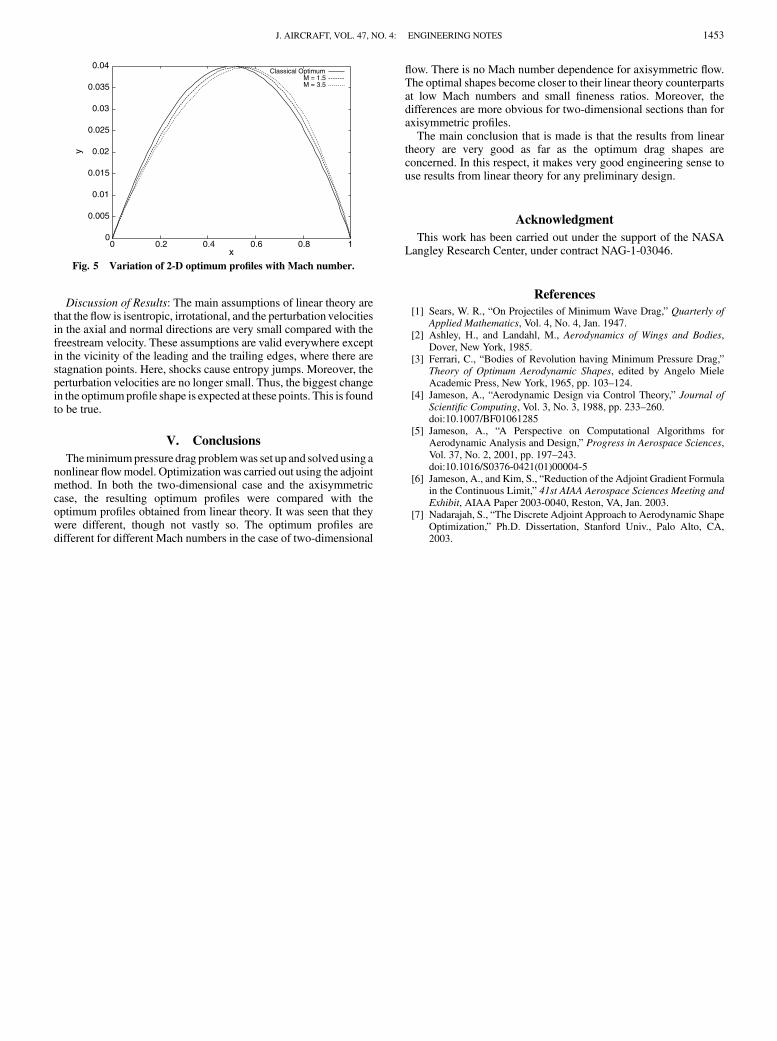
Variation with Mach Number: The optimum profile for 2-D flowchanges with Mach number. The optimum shape for 2 M numbers isshown in Fig. 5. It is seen that the point of maximum thickness isfarther rearward for the higherMach number. This again is consistentwith our earlier argument that the main goal of the nonlinearoptimization is to reduce the magnitude of the leading-edge shock.Such a variation is not observed for axisymmetric optimum profiles.This is due to the fact that the drag coefficient is not sensitive tochanges in Mach number in this case. This can also be seen fromEq. (4).

0

0.005

0.01

0.015

0.02

0.025

0.03

0.035

0.04

0 0.2 0.4 0.6 0.8 1

y

x

Parabolic Profile

Fig. 1 Convergence of the optimization algorithm from a parabolic

initial profile.

0

0.005

0.01

0.015

0.02

0.025

0.03

0.035

0.04

0 0.2 0.4 0.6 0.8 1

y

x

Sears Haack Profile

Fig. 2 Convergence of the optimization algorithm from a Sears–Haack

initial profile.

0

0.005

0.01

0.015

0.02

0.025

0.03

0.035

0.04

0 0.2 0.4 0.6 0.8 1

y

x

Classical TheoryNonlinear Optimum

Fig. 3 Classical and nonlinear optimum profiles for 2-D flow.

0

0.005

0.01

0.015

0.02

0.025

0.03

0.035

0.04

0.045

0 0.2 0.4 0.6 0.8 1

y

x

Classical TheoryNonlinear Optimum

Fig. 4 Classical and nonlinear optimumprofiles for axisymmetric flow.

1452 J. AIRCRAFT, VOL. 47, NO. 4: ENGINEERING NOTES

Discussion of Results: The main assumptions of linear theory arethat the flow is isentropic, irrotational, and the perturbation velocitiesin the axial and normal directions are very small compared with thefreestream velocity. These assumptions are valid everywhere exceptin the vicinity of the leading and the trailing edges, where there arestagnation points. Here, shocks cause entropy jumps. Moreover, theperturbation velocities are no longer small. Thus, the biggest changein the optimumprofile shape is expected at these points. This is foundto be true.

V. Conclusions

Theminimumpressure drag problemwas set up and solvedusing anonlinear flowmodel. Optimization was carried out using the adjointmethod. In both the two-dimensional case and the axisymmetriccase, the resulting optimum profiles were compared with theoptimum profiles obtained from linear theory. It was seen that theywere different, though not vastly so. The optimum profiles aredifferent for different Mach numbers in the case of two-dimensional

flow. There is no Mach number dependence for axisymmetric flow.The optimal shapes become closer to their linear theory counterpartsat low Mach numbers and small fineness ratios. Moreover, thedifferences are more obvious for two-dimensional sections than foraxisymmetric profiles.

The main conclusion that is made is that the results from lineartheory are very good as far as the optimum drag shapes areconcerned. In this respect, it makes very good engineering sense touse results from linear theory for any preliminary design.

Acknowledgment

This work has been carried out under the support of the NASALangley Research Center, under contract NAG-1-03046.

References

[1] Sears, W. R., “On Projectiles of Minimum Wave Drag,” Quarterly ofApplied Mathematics, Vol. 4, No. 4, Jan. 1947.

[2] Ashley, H., and Landahl, M., Aerodynamics of Wings and Bodies,Dover, New York, 1985.

[3] Ferrari, C., “Bodies of Revolution having Minimum Pressure Drag,”Theory of Optimum Aerodynamic Shapes, edited by Angelo MieleAcademic Press, New York, 1965, pp. 103–124.

[4] Jameson, A., “Aerodynamic Design via Control Theory,” Journal of

Scientific Computing, Vol. 3, No. 3, 1988, pp. 233–260.doi:10.1007/BF01061285

[5] Jameson, A., “A Perspective on Computational Algorithms forAerodynamic Analysis and Design,” Progress in Aerospace Sciences,Vol. 37, No. 2, 2001, pp. 197–243.doi:10.1016/S0376-0421(01)00004-5

[6] Jameson, A., and Kim, S., “Reduction of the Adjoint Gradient Formulain the Continuous Limit,” 41st AIAA Aerospace Sciences Meeting and

Exhibit, AIAA Paper 2003-0040, Reston, VA, Jan. 2003.[7] Nadarajah, S., “The Discrete Adjoint Approach to Aerodynamic Shape

Optimization,” Ph.D. Dissertation, Stanford Univ., Palo Alto, CA,2003.

0

0.005

0.01

0.015

0.02

0.025

0.03

0.035

0.04

0 0.2 0.4 0.6 0.8 1

y

x

Classical OptimumM = 1.5M = 3.5

Fig. 5 Variation of 2-D optimum profiles with Mach number.

J. AIRCRAFT, VOL. 47, NO. 4: ENGINEERING NOTES 1453