Sheng-Fang Huang

6.2 Transforms of Derivatives and Integrals. ODEs

Laplace Transform of Derivatives(1)

THEOREM 1

The transforms of the first and second derivatives of ƒ(t) satisfy

Laplace Transform of the Derivative ƒ(n) of Any Order

THEOREM 2

(3)

Example 1Let ƒ(t) = t sin ωt. Then ƒ(0) = 0, ƒ'(t) = sin ωt

+ ωt cos ωt, ƒ'(0) = 0, ƒ" = 2ω cos ωt – ω2t sin ωt. Hence by (2),

Example 2. Proof of Formulas 7 and 8 in Table 6.1This is a third derivation of (cos ωt) and

(sin ωt); cf. Example 4 in Sec. 6.1. Let ƒ(t) = cos ωt. Then ƒ(0) = 1, ƒ'(0) = 0, ƒ"(t) = –ω2 cos ωt. From this and (2) we obtain

Similarly, let g = sin ωt. Then g(0) = 0, g' = ω cos ωt. From this and (1) we obtain

Laplace Transform of the Integral of a Function

Laplace Transform of Integral

THEOREM 3

Let F(s) denote the transform of a function ƒ(t) which is piecewise continuous for t ≥ 0 and satisfies a growth restriction (2), Sec. 6.1. Then, for s > 0, s > k, and t > 0,

(4)

Example 3Using Theorem 3, find the inverse of and

Solution.

Differential Equations, Initial Value Problems

We shall now discuss how the Laplace transform method solves ODEs and initial value problems. We consider an initial value problem

(5) y" = ay' + by = r(t), y(0) = K0, y'(0) = K1

where a and b are constant. In Laplace’s method we do the following three steps:

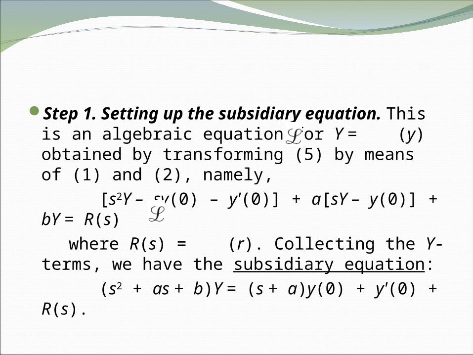
Step 1. Setting up the subsidiary equation. This is an algebraic equation for Y = (y) obtained by transforming (5) by means of (1) and (2), namely,

[s2Y – sy(0) – y'(0)] + a[sY – y(0)] + bY = R(s)

where R(s) = (r). Collecting the Y-terms, we have the subsidiary equation:

(s2 + as + b)Y = (s + a)y(0) + y'(0) + R(s).

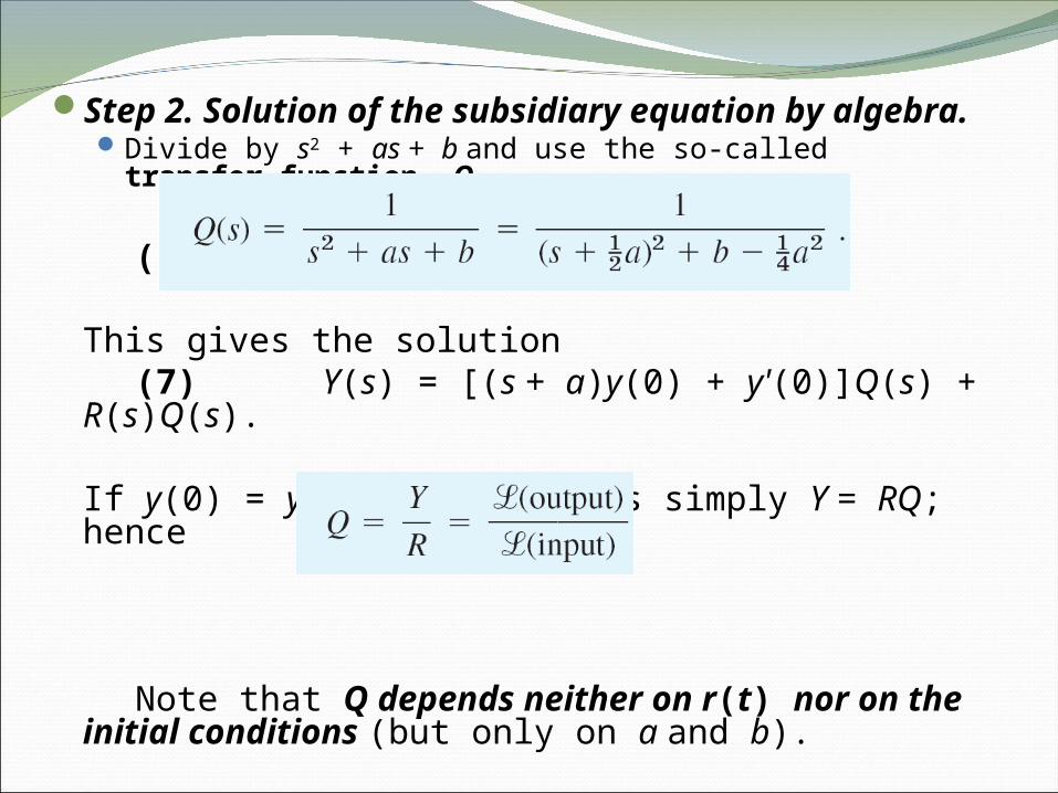
Step 2. Solution of the subsidiary equation by algebra. Divide by s2 + as + b and use the so-called transfer

function, Q

(6)

This gives the solution (7) Y(s) = [(s + a)y(0) + y'(0)]Q(s) +

R(s)Q(s).

If y(0) = y'(0) = 0, this is simply Y = RQ; hence

Note that Q depends neither on r(t) nor on the initial conditions (but only on a and b).

Step 3. Inversion of Y to obtain y =

(Y). Reduce (7) (usually by partial fractions as in

calculus) to a sum of terms whose inverses can be found from the tables (Sec. 6.1 or Sec. 6.9) or by a CAS, so that we obtain the solution y(t) = (Y) of (5).

Example 4Solve y" – y = t, y(0) = 1, y'(0) = 1.Solution.

Step 1. From (2) and Table 6.1 we get the subsidiary equation:

s2Y – sy(0) – y'(0) – Y = 1/s2, thus (s2 – 1)Y = s + 1 + 1/s2.

Step 2. The transfer function is Q = 1/(s2 – 1), and (7) becomes

Simplification and partial fraction expansion gives

Step 3. From this expression for Y and Table 6.1 we obtain the solution

Fig. 115. Laplace transform method

Example 5 Comparison with the Usual MethodSolve the initial value problem y" + y' + 9y = 0, y(0) = 0.16,

y'(0) = 0.Solution.

Advantages of the Laplace Method1. Solving a nonhomogeneous ODE does

not require first solving the homogeneous ODE (Example 4).

2. Initial values are automatically taken care of (Examples 4 and 5).

3. Complicated inputs r(t) (right sides of linear ODEs) can be handled very efficiently, as we show in the next sections.

Example 6 Shifted Data ProblemsThis means initial value problems with

initial conditions given at some t = t0 > 0 instead of t = 0. For such a problem set t = + t0, so that t = t0 gives = 0 and the Laplace transform can be applied. For instance, solve

We have t0 = and we set t = . Then the problem is

Solution:

6.3 Unit Step Function. t-ShiftingUnit Step Function (Heaviside Function) u(t –

a)The unit step function or Heaviside

function u(t – a) is 0 for t < a, and is 1 for t > a, in a formula:

(1)

Figure 117 shows the special case u(t), which has its jump at zero, and Fig. 118 the general case u(t – a) for an arbitrary positive a.

Fig. 117. Unit step function u(t)

Fig. 118. Unit step function u(t – a)

The unit step function is a typical “engineering function” made to measure for engineering applications, which often involve functions that are either “off” or “on.”

Multiplying functions ƒ(t) with u(t – a), we can produce all sorts of effects.

Fig. 119. Effects of the unit step function: (A) Given function. (B) Switching off and on. (C) Shift.

Fig. 120. Use of many unit step functions.

Time Shifting (t-Shifting): Replacing t by t – a in ƒ(t)

Second Shifting Theorem; Time Shifting

THEOREM 1

If ƒ(t) has the transform F(s), then the “shifted function”

(3)

has the transform e-asF(s). That is, if {ƒ(t)} = F(s), then

(4)

Or, if we take the inverse on both sides, we can write

(4*)

Example 1 Use of Unit Step FunctionsWrite the following function using unit

step functions and find its transform.

Solution. Step 1. In terms of unit step functions,

Indeed, 2(1 – u(t – 1)) gives ƒ(t) for 0 < t < 1, and so on.

Step 2. To apply Theorem 1, we must write each term in ƒ(t) in the form ƒ(t – a)u(t – a).

If the conversion of ƒ(t) to ƒ(t – a) is inconvenient, replace it by

(4**) (4**) follows from (4) by writing ƒ(t – a) =

g(t), hence ƒ(t) = g(t + a) and then again writing ƒ for g. Thus,

Fig. 121. ƒ(t) in Example 1

Example 2 Application of Both Shifting Theorems. Inverse Transform

Find the inverse transform ƒ(t) of

Solution.

Fig. 122. ƒ(t) in Example 2