Engineering and Research Center Bureau of Reclamation · Measuring Water Velocity with an Ultrasonic Flowmeter 7 ... A conclusion of the study was: ... computed from the venturi meter

i

REC-ERC-72-32

J. C. Schuster

Engineering and Research Center

Bureau of Reclamation

September 1972

D~ . T ::-· -·~ . • . ,- TO ' - ·• -• . _ ...... ,J FILE

E><TR/\

MS-230 (8-70) Bureau of Reclamation

1. REPORT NO .

REC-ERC-72-32 4. TITLE AND SUBTITLE

Measuring Water Velocity with an Ultrasonic Flowmeter

7. AUTHOR(S)

J. C. Schuster

9. PERFORMING ORGANIZATION NAME AND ADDRESS

Engineering and Research Center Bureau of Reclamation Denver, Colorado 80225

12. SPONSORING ~GENCY NAME AND ADDRESS

Same

15 . SUPPLEMENTARY NOTES

16. ABSTRACT

5. REPORT DATE

Sep 72 6 . PERFORMING ORGANIZATION CODE

8. PERFORMING ORGANIZATION REPORT NO .

R EC-E RC-72-32

10 . WORK UNIT NO .

11. CONTRACT OR GRANT NO.

13. TYPE OF REPORT AND PERIOD COVERED

14. SPOl'ISORING AGENCY CODE

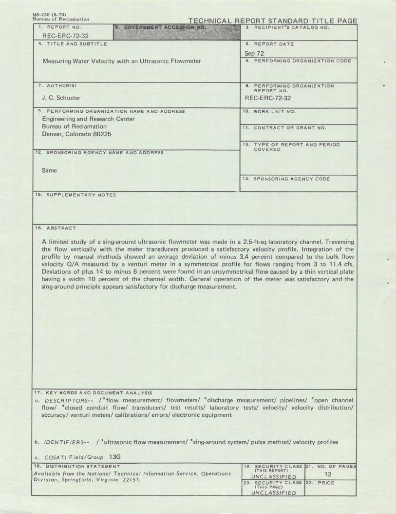
A limited study of a sing-around ultrasonic flowmeter was made in a 2.5-ft-sq laboratory channel. Traversing the flow vertically with the meter transducers produced a satisfactory velocity profile. Integration of the profile by manual methods showed an average deviation of minus 3.4 percent compared to the bulk flow velocity Q/A measured by a venturi meter in a symmetrical profile for flows ranging from 3 to 11.4 cfs. Deviations of plus 14 to minus 6 percent were found in an unsymmetrical flow caused by a thin vertical plate having a width 10 percent of the channel width. General operation of the meter was satisfactory and the sing-around principle appears satisfactory for discharge measurement.

17. KEY WORDS AND DOCUMENT ANALYSIS

a. DESCRIPTORS- - I *flow measurement/ flowmeters/ * discharge measurement/ pipelines/ * open channel flow/ *closed conduit flow/ transducers/ test results/ laboratory tests/ velocity/ velocity distribution/ accuracy/ venturi meters/ calibrations/ errors/ electronic equipment

b. IDENTIFIERS-- I *ultrasonic flow measurement/ *sing-around system/ pulse method/ velocity profiles

c. COSATI Field/Group 13G 18. DISTRIBUTION STATEMENT

Available from the National Technical Information Service , Operations Division , Springfield, Virginia 22151.

19 . SECURITY CLASS (TH IS RE PORT)

UNCLASSIFIED 20 . SECURITY CLASS

(THIS PAGE)

UNCLASSIFIED

21 . NO . OF PAGE

12 22. PRICE

REC-ERC-72-32

MEASURING WATER VELOCITY WITH

AN ULTRASONIC FLOWMETER

by J. C. Schuster

September 1972

Hydraulics Branch Division of General Research Engineering and Research Center Denver, Colorado

UNITED STATES DEPARTMENT OF THE INTERIOR Rogers C. B. Morton Secretary

* BUREAU OF RECLAMATION Ellis L. Armstrong Commissioner

ACKNOWLEDGMENT

This report prepared in the Hydraulics Branch was possible because of the loan of an ultrasonic flowmeter by Badger Meter, Inc., Precision Products Division. Laboratory measurements and parts of the analysis were made by Mr. Shih-Hsiung Hsu, Engineer, Taiwan, and Mr. Sei Fujimoto, Public Works Research Institute, Japan, under the author's supervision.

The information contained in this report regarding commercial products or firms may not be used for advertising or promotional purposes and is not to be construed as an endorsement of any product or firm by the Bureau of Reclamation.

Figure

9

10 11

CONTENTS-Continued

Ultrasonic flowmeter velocity profiles (unsymmetrical distribution) . . . . . . . . . . . . . .

Ultrasonic path and wake behind plate normal to flow Ultrasonic path and approximate velocity distribution

behind plate normal to flow . . . . . . . .

ii

Page

8 9

10

CONTENTS

Introduction Laboratory Installation Measurement Procedures Measurement Results

Symmetrical Velocity Distribution

Velocity traversing Traverse results

Unsymmetrical Velocity Distribution

Velocity distortion Velocity traversing Traverse results

Conclusions Application

Table

2 3

4

Figure

1 2 3 4

5 6

7 8

LIST OF TABLES

Discharge and velocity comparisons for ultrasonic flowmeter measurements in a symmetrical velocity distribution . . . . . . . . . . . . .

Venturi meter calibration check Deviations in average velocities computed by single

and multipoint methods . . . . . . . . Discharge and velocity comparisons for ultrasonic flow

meter measurements for unsymmetrical velocity distribution . . . . . . . . . . . . . . .

LIST OF FIGURES

Meter installation forms . . . . . . . . . . . V installation form for laboratory . . . . . . . . Laboratory channel installation of ultrasonic flowmeter Transducer face raised above a still water surface

in channel Ultrasonic flowmeter installation . . . . . . Ultrasonic flowmeter velocity profiles (symmetrical

distribution) . . . . . . . . . . . . . Increase in surface waves with increasing flow Average velocity-Ultrasonic flowmeter and venturi

meter discharge . . . . . . . . . . .

Page

1 1 2 4

4

4 4

8

8 8 8

10 11

6 6

7

9

1 1 2

2 3

4 5

5

Figure 3. Laboratory channel installation of ultrasonic flowmeter. (al. Transducer section of channel. Photo PX-D-72010

Figure 4 . Transducer face raised above a still water surface in channel. Photo PX-D-72011

the two transducers. Discharges through the channel were measured by volumetrically calibrated venturi meters.

Although discharge measurement was of primary interest in the pipeline studies, velocity distribution was of primary interest in the channel studies. The company modified the meter circuitry in the time between the pipe and channel studies. A 4- to 20-milliampere (ma) current was previously related to a 0- to 20-cubic feet per second (cfs) (0- to 0.57-cms) discharge. The

2

conversion of the meter related in linear form the 4- to 20-ma current to a 0- to 3-feet per second (fps) (91.4 cm/sec) maximum velocity for the channel.

The 0- to 20-ma current would normally drive a velocity recorder that was not sufficiently responsive to obtain the desired accuracy in the laboratory measurements. In the laboratory measurements the current was converted to a 0.4- to 2.0-volt signal by placing a 100 ohm ±0.05 percent resistor across the meter output terminals. The voltage was desirable because integrating digital voltmeters and not current meters were available. The data acquisition system was thus assembled to average a voltage related to the velocity of flow, Figure 5.

MEASUREMENT PROCEDURES

An arbitrary depth of 2 feet (61 cm) was selected in the 2.5-foot-deep flume for discharges ranging from 3 cfs (0.08 ems) to 11.4 cfs (0.33 ems). The mean velocities for this range of flow were about 0.6 fps ( 18 ems) to 2.2 fps (67 ems). Velocities were measured from near the floor of the flume to near the water surface by raising the transducers and integrating the

INTRODUCTION

The meter uses two ultrasonic transceivers strapped to the outside of a pipe wall or submerged in an open channel, Figure 1. Pulses of ultrasonic energy from the transmitter propagate through the liquid and across to the receiver. The reception of a pulse triggers the next pulse from the transmitter. A continuous "singaround" frequency is generated in this manner. After about 2 seconds the direction of propagation is reversed. When transmitted in the downstream direction, the speed of the fluid increases the speed of the ultrasonic pulse, reduces the transit time, and increases the sing-around frequency. When transmitted upstream, the pulses are opposed by fluid motion and the sing-around frequency is reduced. The measured frequency difference is proportional to fluid velocity. This frequency differencing procedure removes the influence of the value of the sonic velocity in a metered liquid of uniform quality.

FACE

TRANSDUCER B

V INSTALLATION FORM Z INSTALLATION FORM

Figure 1. Meter installation forms

The accuracy of discharge measurement of the ultrasonic flowmeter in a 2-foot-diameter pipeline was previously studied in the Hydraulics Branch, 1 • One of the stated advantages of the meter was, that knowing the geometry and coating materials of a steel pipeline, the transducers could be mounted on the outside surface of the pipe to measure the discharge. The thesis study was performed with the transducers mounted on the outside of the pipe in two configurations, Figure 1.

A conclusion of the study was: "In future installations the ultrasonic flowmeter's transducers should be installed in direct contact with the fluid stream. The

largest source of error in installations with the transducers mounted on the outside of the conduit can be in transmitting the sound pulse through the conduit's wall."

The study of the meter, to determine how well the meter could be used for integrating the discharge was continued in an open channel and is discussed in this report. The face of the transducer as suggested in the thesis was placed in contact with the flowing water through a vertically movable side of the channel, Figure 2.

TRANSDUCERS IN MOVABLE~

d;q }

\ I \ I

\ I \ I

Figure 2. V installation form for laboratory

LABORATORY INSTALLATION

The ultrasonic flowmeter was installed to measure the velocity in horizontal planes in a 2.5-foot (76-cm) wide channel, Figure 3.

The channel, about 55 feet long, contained a calming section 40 feet upstream from the meter location. One side of the channel, containing the flush-mounted transducers, could be raised or lowered to position the transducers vertically for velocity measurement, Figure 4.

An 11-thread per inch stem and handwheel were used to accurately position the slide with respect to 2 pointers and elevation scales. Channel flow depths were obtained from a hDok gage in a stilling well connected to a pressure tap. The pressure tap was in the floor on the channel longitudinal centerline midway between

1 Kitchen, M. L., "Ultrasonic Flowmeter for Fluid Measurement," Master of Science Thesis, Department of Civil and Environmental Engineering, University of Colorado, 1971.

comparable to those requiring measurement in distribution systems.

MEASUREMENT RESULTS

Symmetrical Velocity Distribution

Velocity traversing. - Preliminary measurements showed a good average of the voltage (velocity) could be obtained normally from ten 100-second samples. When large variations were noted, the number of samples was increased to 30 or more. Traverses were made for discharges of approximately 3, 5, 8, 9, and 11 cfs (0.08, 0.14, 0.23, 0.26, and 0.31 ems). The depth for each discharge was adjusted as closely as possible to 2.0 feet (61 cm).

Traverse resu/'ts. - In general the velocity distributions evidenced a bluntness of profile, Figure 6. Detailed studies were made near the floor and water surface in an attempt to define the distribution of velocity. The studies were not particularly successful because of multiple reflections of the ultrasonic pulses from the floor and uneven water surface. Success was better for the small flows than the large ones for the positions near the water surface because of fewer waves, Figure 7.

The distribution curves were integrated over the depth of the flow to find the average velocity. In the horizontal at the elevation of the transducers the flowmeter measures an average line velocity along the V path. Thus, a vertical integration of the velocity curve should produce the average velocity for the cross section.

The velocity curves were extrapolated near the floor and water surface because difficulties were encountered in measuring close to the upper and lower surfaces. The exact origin of the pulse from the transducer face was not known. Therefore, the vertical center of the narrow (0.172-foot, 6.2-cm) side of the transducer (intersection of diagonals) was used as a reference elevation for the velocity measurements. An integration of the curves was made weighting the slight deviations of width in the vertical of the channel cross section. Corrections were made for path length variations in the order of 1/250.

The results showed the flowmeter average velocity to be slightly below that of the bulk flow velocity computed from the venturi meter discharge, Table 1 and Figure 8. There was no apparent regularity to the differences in average velocity between the ultrasonic flowmeter and venturi except the flowmeter did

4

2.0 1 .......,,,.__ 1

~ \

,.:_ I - -.......

1.8

1.6

~

~

\ , 1.4

.:: i.i i.i LL

II) II) II) IJ)

LL LL If LL LL (,) (,) (,) (,)

on ,n (,)

iii .., GO 0 t\i on ,..: ai -1.2

z 0 j: < > i.i

1.0 ..I i.i

It: i.i (,)

=> Q .8 II)

z < It: ...

. 6 • J I

I

.4 '

.2

TRANSDUCE~

) HE~ I

-

~ /I /I ~1--; X

I , I /' /

I/, FLOOR

0 2

VELOCITY (FPS)

Figure 6. Ultrasonic flowmeter velocity profiles (symetricel distribution I.

underregister the venturi discharge by an average of about -3.4 percent.

A volumetric recalibration of the venturi meters was made over the range of flows used in the ultrasonic flowmeter measurements, Table 2. The average difference between the laboratory standard tables and the volumetric tank was 0.28 percent. The difference ranged from a maximum of 0.64 percent at 3 cfs to a minimum of 0.02 percent at 10 cfs.

Near the conclusion of the tests, the voltage output (corresponding to the 20-ma current) could not be adjusted to the full stated value. In place of 2 volts, the

Figure 5. Ultrasonic flowmeter installation . (a). T ransducer section (b) . Flowmeter electronics. (c). Integrating digital voltmeter. (d) . Tape printer. Photo PX-D-72009

flowmeter output voltage. The increments between vertical positions of the transducers were varied dependent on the curvature of the velocity distribution.

The flowmeter operates on a "sing-around" period with a train of ultrasonic pulses travelling upstream for about 2 seconds and then downstream in the flow for the same period. The difference in frequency caused by the water velocity is used to compute the velocity V of the flow, 2 •

[ 1 C 2 J

V = 28 fo tan 0J:lf

I length of water path B width of channel C sound velocity in water f0 = sing-around frequency in still water 0 = acute angle of sound path with channel

centerline Af = frequency difference upstream to downstream

A velocity measurement is completed in about 5 seconds allowing 1 second for switching pulse direction and calculating the velocity .

The upstream-downstream sing-around period is approximately 5 secpnds. Thus, a register in the flowmeter is updated each 5 seconds and the current or voltage represents the average velocity during the period.

The integrating digital voltmeter sampled the output voltage of the flowmeter for time periods that were variable. Times could be varied from 1 second to large multiples of seconds by using a crystal oscillator. A 100-second period of integration was selected because of the 5-second sing-around period. Thus, each 100 seconds was an average of approximately 20 singaround periods or samples. Multiples of the 100:second integration periods were used in measuring the average velocity for each elevation plane of the meter transducers.

Continual records were made manually of the Venturi meter manometer differential and the depth of flow from the hook gage. Thus, 25 to 30 manometer and gage readings were acquired during the velocity traverse. Although the laboratory is not equipped with a constant-head tank, the pumping system is relatively steady. Flows produced by the system should be

2 Suzuki, H., et al., "Ultrasonic Method of Flow Measurement in an Open Channel," Water Power (British), May/June 1970, pages 213-218.

3

• )K

3 cfs

Flow

11.4 cfs

Figure 7. Increase in surface waves with increasing flow. Photos PX-D-72013 and PX-D-7212.

II)

Q. >- 2 1----+-----+------+----#'-r---l------1 "- f,-

- u >- 0 f,- _,

g~ ~~ wZ "'0 :~ W a: I 1----+----.ff----+----+---1-------1

~ IB f,-

~

"::,

0

WIDTH OF FLUME• 2.510 FT. DEPTH OF WATER • 2.00 FT. DISCHARGE RANGE 3-11.4 CFS TRANSDUCERS IN V CONFIGURATION

AVERAGE VELOCITY (FPS I - VENTURI Q/A

Figure 8 . Average velocity-Ultrasonic flowmeter and venturi meter discharge.

range was about 1.984 to 1.990 on various days of measurement. Based on this range of voltage, the possible error at full scale, 3 fps, would range from 0.8 to 0.5 percent. No difficulty was encountered in adjusting the zero end of the 0- to 3-fps scale. A 0.4

5

volt (4 ma) adjustment at zero was essentially stable throughout the measurements.

At 0.6-fps velocity (3 cfs, 0.08 ems) the Venturi meter calibration indicated the possibility of a positive difference of 0.6 percent. An ultrasonic velocity measuring error of 0.1 percent low (0.6/3.0 x 0.5) might also be possible. The sum of these errors, 0. 7 percent, is much less than -3.4 percent, Table 1. At 2-fps velocity (11 cfs, 0.31 ems) the error in the Venturi calibration was close to zero but the ultrasonic velocity indication could have been low by about 0.4 percent. A -2.52 percent difference was measured in comparing the ultrasonic and Venturi indicated velocities.

An additional source of error in the analysis was in the integration of the velocity distribution curves. The velocity curves were interpolated by straight lines between measured velocities. Extrapolations were made near the channel bottom and water surface by directions indicated from velocities adjacent to these boundaries. Slight modifications of the curves in these areas would produce slight changes in the average velocity computed from the integration. In most positions on the velocity curves, a smooth curve interpolation (least squares fit or other) would have a balancing effect on the area to produce essentially the same average.

Water depth (ft.)

Ultrasonic Ou

Flow-Meter Vu

Volumetric a Calibration V

Discharge ratio Ou/0

DIFFERENCE (%)

Table 1

COMPARISON INTEGRATION AVERAGE AND BULK FLOW VELOCITIES

AND DISCHARGES

MEASUREMENT

1 2 3 4 5 Average

2.00 2.00 2.03 2.00 2.00

2.91 7.81 11.10 5.35 9.05

0.58 1.56 2.18 1.07 1.80

3.02 8.01 11.39 5.55 9.50

0.60 1.60 2.24 1.11 1.89

0.966 0.975 0.975 0.964 0.952

-3.4 ·2.5 -2.5 -3.6 -4.8

Table 2

VENTURI METER CALIBRATION CHECK

April 18, 1972

Venturi meter Calibration tank Comparasion

-3.4

~ s discharge (Qv) discharge (Oc) Qv/Qc Deviation%

1 3.003 3.0215 0.9939

I 2 3.020 3.0395 0.9936 3 3.007 3.0234 0.9946

Average 3.010 3.0281 0.9940 0.60

1 7.994 8.0081 0.9982

II 2 7.988 8.0065 0.9977 3 7.990 8.0074 0.9978

Average 7.991 8.0073 0.9980 0.20

1 10.137 10.1410 0.9996

II I 2 10.140 10.1007 3 10.136 10.1380 0.9998

Average 10.136 10.1395 0.9997 0.03

Average of I, II, & Ill 0.9972 0.28

6

Remarks

Width of flume = 2.510

a in cfs Vin fps

Remarks

8" SE Venturi

12" SE

12" SE Water overflow into waste pipe Average 1 & 3 only

that a satisfactory average could have been obtained by placing the transducers at three or four elevations by the Gauss Method and five by the Chebyshef method. Placing transducers at specified elevations or traversing to stop at these elevations apparently would provide a sufficient number of velocities (averaged with time) to compute an average velocity for the cross section.

Unsymmetrical velocity distribution

Velocity distortion. - Optimum locations for installing an ultrasonic flowmeter do not always occur in open channels. Therefore, this study was extended to include an unsymmetrical velocity distribution within the cross section of measurement. The distortion allowed a limited evaluation of the ultrasonic flowmeter capabilities of averaging nonuniform distribution.

The nonuniform velocity distribution was caused by a vertical thin plate obstruction. The plate was attached to the wall 2.92 feet (89 cm) upstream from the centerline of the transducer pair on the opposite side of the channel. The projection of the plate was 10 percent of the 2.5-foot-wide channel.

Velocity traversing. - A 100-second time averaged measurement of the voltage (velocity) was taken again as a base sample. Velocity variations caused by the unsteady flow downstream from the plate were larger than those occurring for the uniform distribution. A preliminary study indicated that acceptable averages could be obtained from about sixteen 100-second integrations of the output voltage from the flowmeter. Traverses were made for discharges of about 3, 5, 8, and 11 cfs (0.08, 0.14, 0.23, and 31 ems) at a depth adjusted as close as possible to 2.0 feet (61 cm).

Traverse resu/'ts. - Extreme care was taken in measuring the velocity distribution, but the profile was considerably more irregular than for the symmetrical distribution, Figure 9. The profiles remain relatively blunt but show gradually increasing velocity from top to bottom of the channel. Again difficulties were encountered in measuring velocities near the water surface and floor thus defining the distribution was difficult. Wave heights were increased with increased flow as the surface adjusted to the circulation caused by the plate, Figure 10.

Extrapolations of the profiles were made near the water surface and floor without an elaborate attempt

8

2.0

1.8

1.6

1.4

I-ILi ILi LL.

1.2 z 2

,~ ~\ ,-l-"°MAX.

J \ \

\ "' '

f\ ' I\ I

I \

~1 , Cl),

LL.

~ ff! 0

0 0 'II'. , 011

I I I-<( > ILi

1.0 ..I ILi

Q; ILi 0 ::, Q .8 U) z <( Q;

\

\ I-

.6 \ \

\ ' .4

TRANSDUCER

.2 H~

_J

J .,,..,., ~

X / -~ I I I

I _,I

FLOOR I I ~' 0 2

VELOCITY (FPS)

Figure 9. Ultrasonic flowmeter velocity profiles (unsymmetrical distribution).

at definition. Average velocities obtained from the profiles by a weighted arithmetic and planimeter integration and by venturi differed by percentages ranging from plus 14 percent at 3 cfs to about minus 6 percent at 11 cfs. The change from overregistration to underregistration came between the 3 and 4 cfs discharges, Table 4. The increased irregularity between the symmetrical and unsymmetrical profiles show the effect of adding the thin-plate obstruction, Figures 6 and 9. The shift in profile is also evidenced in the change in ratio of the average velocities.

The cause of the slight decrease in velocity between about 0.3 and 0.7 feet (9 and 21 cm) could not be found, Figure 6. Inspecting and measuring the channel width showed a slight outward dishing of the plastic windows in the channel sidewalls. The maximum deflection occurred at about 1.2 feet, midway from top to bottom. Velocities through this horizontal section of the channel would be slightly lower but did not coincide with the elevation indicated by the meter. Repetition of the velocity measurements between 0.3 and 0.7 feet confirmed the indentation.

A limited analysis was made of the velocity distribu· tion curves by single and multipoint selection of transducer position. In open channel discharge measurements by current meter an elevation, 0.6 of the depth below the water surface, is often selected as a

point of average velocity. An average velocity is sometimes determined from measurements at 0.2 and 0.8 of the depth, 0 = A(Vo.2 + Vo.8)/2. These methods were applied to the velocity distribution curves of Figure 6, Table 3. For 3, 8, and 11.4 cfs, the 0.6 depth velocity differed from the average of the integral of the complete traverse by plus 5.2, plus 5.5, and plus 2. 7 percent. The values for the average of 0.2 and 0.8 velocities were only slightly higher than the integrated average by plus 0.2, plus 1.35, and plus 1.51 percent. A 10-point equally weighted method of integrating the velocity gave nearly the same averages as the full integration.

Two quadrature methods, Gauss unequal weighting and Chebyshef using equal weighting of the velocities, were applied to the velocity profiles, 3 • The results showed

Table 3

No. of Methods Stations

1 Simple 2 Average 10

2 Gauss 3

4 5

2 3 4 5

Chebyshef 6 7

8 9

10

DEVIATIONS IN AVERAGE VELOCITIES COMPUTED BY SINGLE AND MULTIPOINT METHODS

Percent of deviation'

DISCHARGE CFS

3 8 11.4 Average2

+5.17 +5.52 +2.70 4.46 +0.17 +1.35 +1.51 1.01 +0.02 +0.06 +0.14 0.07

+0.85 +1.86 +1.37 1.36 +0.38 +0.19 +0.64 0.40 +0.26 - 0.26 +0.09 0.20 +0.03 +0.19 - 0.41 0.21 +0.85 +1.86 +1.37 1.36 +0.71 +0.71 +1.33 0.92 +0.47 +1.15 +0.92 0.85 +0.14 +0.19 +0.14 0.16 +0.16 +0.32 +0.27 0.25 +0.09 - 0.06 -0.05 0.07

+0.05 +0.13 - 0.32 0.17 - 0.05 +0.26 - 0.09 0.13 +0.21 +0.32 - 0.14 0.22

Remarks

Vo.6 !V 0.2 + v o.81 Based on one-tenth depth measurements (0.2 foot)

1 Percent deviation in ratio to integrated average velocity from distribution curve measured by Ultrasonic Flowmeter.

2 Average error equal to the average value of the absolute errors for the three discharges.

3 "FLUID METERS, Their theory and Application," Sixth Edition 1971, The American Society of Mechanical Engineers, New York, New York.

7

UF (Wt-Arith)

UF (Planimeter)

VENTURI

3 cfs

11.4 cfs

Figure 10. Ultrasonic path and wake behind plate normal to flow. Photos PX-D-72015 and PX-D-72014.

Table 4

DISCHARGE AND VELOCITY COMPARISONS FOR ULTRASONIC FLOWMETER MEASUREMENTS IN AN UNSYMMETRICAL VELOCITY DISTRIBUTION

MEASUREMENT #1 MEASUREMENT #2 MEASUREMENT #3 MEASUREMENT #4

Q % % % %

cps 3.49 4.64 7.58 10.81 114 91 95 95

V fps 0.69 0.92 1.53 2.15

Q cps 3.47 4.36 7.77 10.54

V 114 86 96 92

fps 0.69 0.87 1.55 2.10

Q cps 3.05 5.05 8.06 11.4

V 100 100 100 100

fps .60 1.01 1.61 2.27

9

Two-dimensional studies have been made of the wake downstream from a flat plate normal to the flow, 4 •

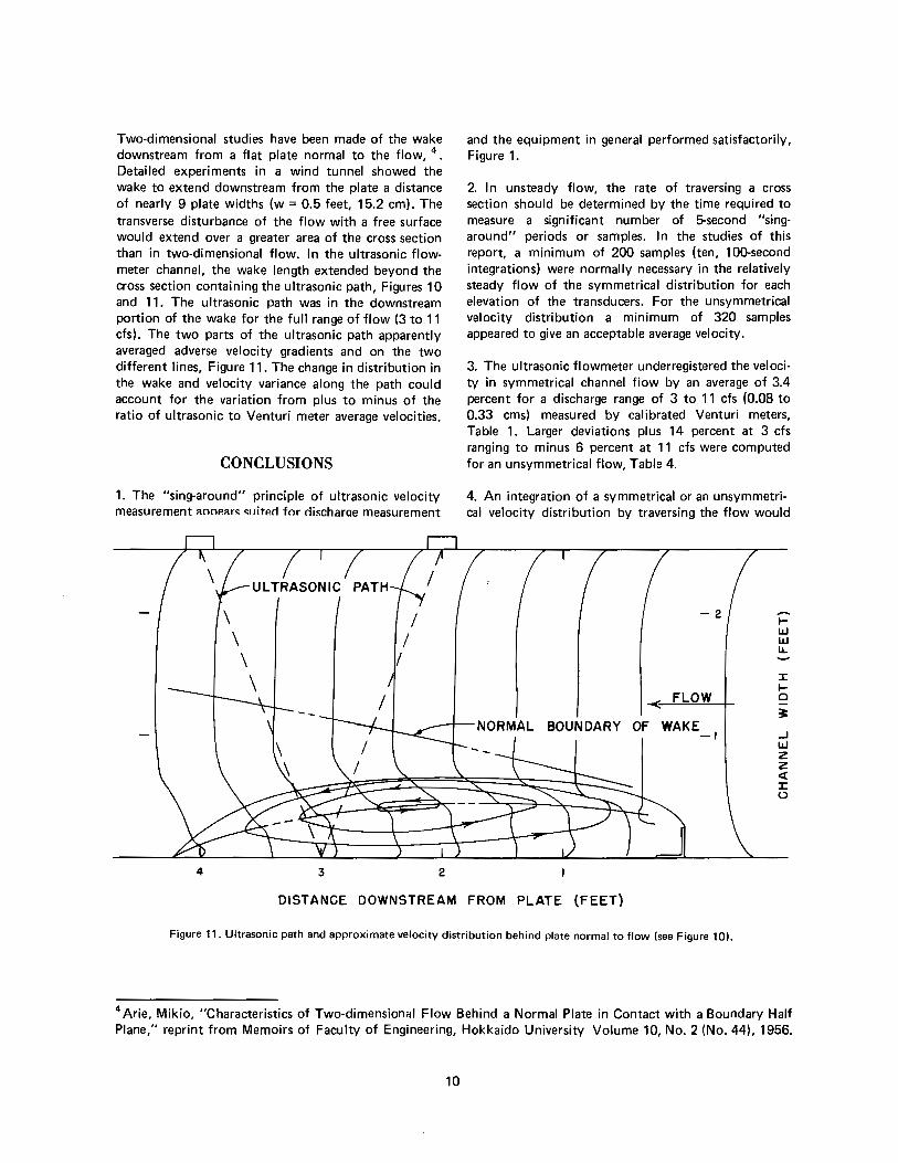
Detailed experiments in a wind tunnel showed the wake to extend downstream from the plate a distance of nearly 9 plate widths (w = 0.5 feet, 15.2 cm). The transverse disturbance of the flow with a free surface would extend over a greater area of the cross section than in two-dimensional flow. In the ultrasonic flowmeter channel, the wake length extended beyond the cross section containing the ultrasonic path, Figures 10 and 11. The ultrasonic path was in the downstream portion of the wake for the full range of flow (3 to 11 cfs). The two parts of the ultrasonic path apparently averaged adverse velocity gradients and on the two different lines, Figure 11. The change in distribution in the wake and velocity variance along the path could account for the variation from plus to minus of the ratio of ultrasonic to Venturi meter average velocities.

CONCLUSIONS

1. The "sing-around" principle of ultrasonic velocity measurement anm,im; i:uitP.rl for rlii:charqe measurement

I I

I

and the equipment in general performed satisfactorily, Figure 1.

2. In unsteady flow, the rate of traversing a cross section should be determined by the time required to measure a significant number of 5-second "singaround" periods or samples. In the studies of this report, a minimum of 200 samples (ten, 100-second integrations) were normally necessary in the relatively steady flow of the symmetrical distribution for each elevation of the transducers. For the unsymmetrical velocity distribution a minimum of 320 samples appeared to give an acceptable average velocity.

3. The ultrasonic flowmeter underregistered the velocity in symmetrical channel flow by an average of 3.4 percent for a discharge range of 3 to 11 cfs (0.08 to 0.33 ems) measured by calibrated Venturi meters, Table 1. Larger deviations plus 14 percent at 3 cfs ranging to minus 6 percent at 11 cfs were computed for an unsymmetrical flow, Table 4.

4. An integration of a symmetrical or an unsymmetrical velocity distribution by traversing the flow would

-2 ...... 1-LIJ LIJ IL. -

~ FLOW

-r-NORMAL BOUNDARY OF WAKE

:c lo ;:

J LIJ z z 4: :c 0

-I

4 3 2

DISTANCE DOWNSTREAM FROM PLATE (FEET)

Figure 11. Ultrasonic path and approximate velocity distribution behind plate normal to flow (see Figure 10).

4 Arie, Mikio, "Characteristics of Two-dimensional Flow Behind a Normal Plate in Contact with a Boundary Half Plane," reprint from Memoirs of Faculty of Engineering, Hokkaido University Volume 10, No. 2 (No. 44), 1956.

10

produce the optimum discharge measurement. The meter should be placed in a symmetrical velocity distribution or means provided for in-place calibration for unsymmetrical distributions.

5. Accurate average velocities would not be measured in short periods in unsteady flow.

6. The flowmeter appeared capable of measuring the velocity to a distance of about 0.1 foot (3 cm) of the floor and water surface in a 2.5-foot flume. Multiple reflections caused large variances in velocity at lesser distances.

7. Automation of an ultrasonic flowmeter measuring system for traversing would require extrapolation in the computer section to adjust the velocity profile near the water surface and channel bottom for calculating the discharge.

8. The effect of the variance at the boundaries on computing the total flow in relatively deep channels with quiet water surfaces would be minimal.

9. The flowmeter computer should be capable of accepting an input related to depth and thus, flow area changes for accurately computing discharge.

10. Transducers located at 0.6 of the depth from the surface in the laboratory channel did not measure a satisfactory average velocity.

11. Transducers located at 0.2 and 0.8 depth possibly could produce a satisfactory average velocity depending on the symmetry of flow and the measurement· requirements.

12. Multipoint locations of transducers or measurements by a single pair of transducers moved to elevations defined by Gauss and Chebyshef methods of integration would produce satisfactory average velocities (each velocity time averaged at elevation).

13. Measurements of the velocity and computing the discharge in unsymmetrical flows or in those having adverse velocity gradients are subject to greater errors.

14. A "Z" configuration of the transducers in place of the "V" might reduce the error in measuring the average velocity of flow for the thin plate because averaging would be in one instead of two ultrasonic paths. The "Z" configuration or reflective targets could be used in a trapezoidal channel to minimize loss of signal from the sloping sides.

11

15. No major difficulties were encountered with the electronic circuitry of the meter in the 2-month operating period. Long term operating characteristics were not available from this study.

16. A 0.5 to 0.8 percent reduction in the full-scale output of the meter was encountered near the end of the study.

17. A stainless steel plate cemented to the face of the epoxy embedding the transducer crystals appeared to retain integrity throughout the study.

18. A transducer smaller than the 2.1 inch (5.3 cm) by 2.9 inch (7.4 cm) probably would have improved the resolution of the velocity measurements.

19. An instrument shelter for environment and vandalism control would be necessary for the electronics enclosure (Wall space 29 inches high, 22.5 inches wide and 12-inches deep with a 23-inch door radius) and for a circular chart recorder if desired (19 by 14 by 9 inches). Analog recording and digital totalizing of the flow could be done on-site or be transmitted by wire or radio to a remote site.

APPLICATION

Ultrasonic flowmeters can be applied to measuring small and large flows in open-channel and closed-conduit systems. The accuracy of the measurement depends on positioning the transducers to measure a true average velocity in either open- or closed-conduit flow. A measurement of (plus or minus 2 percent) accuracy may be obtained by applying a correction factor to the velocity measurement from a single pair of transducers in a pipe having a fully developed turbulent velocity distribution. Possibly four pairs of transducers or a traversing pair are required for accurate measurements in a conduit or channel with unsymmetrical distribution. The metering method can be applied to flows varying over a wide range in open channels, to systems designed for a minimum head loss (such as power and pumping plants), to large capacity turnouts that may require multiple Venturi meters to measure the flow range, and to :iystems having main supplies controlled by automatic or supervisory means. Application of the ultrasonic flowmeter or other meters requiring electrical power should consider the cost of supplying the power in evaluating the meters.

The ultrasonic method of velocity and flow measurement can be applied to pipes and cross-sectional shapes

of natural and artificial channels. The complexity of traversing mechanisms or supports for locating fixed transducers in channels will vary with the shape of the cross section and the required accuracy of the flow measurement.

Ultrasonic flowmeter systems have a basic cost for the electronics and a pair of transducers. Costs of the installations will be governed by the complexity of the shape, the number of transducer pairs, and the scanning equipment needed to produce the required discharge indication or totalization.

An ultrasonic flowmeter could be the only satisfactory means of measurement at some structures, (e.g. large channels or conducts, low-head loss requirement) and thus, the cost must be justified on the need for the

12

measurement or on the savings of water. Cost comparisons can be made when other devices are available. For example in a steel pipeline having flow lengths comparable to that required for a Venturi meter, a basic ultrasonic flowmeter system should meet the stated accuracy of the manufacturer. Under these conditions at the time of this report, the cost of the meter was greater than the cost of a standard Venturi meter for 24-inch and smaller sizes and less than the cost above this size. Installation costs for the ultrasonic flowmeter should be less than that for a Venturi meter in interchangeable sizes, because the attachment of the transducers to the outside of a steel pipe wall or to a metal section of channel recommended by the manufacturer is a relatively simple process. Secure attachment and maintained contact of the transducers should preserve the accuracy of the system.

Table II

QUANTITIES AND UNITS OF MECHANiCS

Multiply

Grains (1/7,000 lb) ...•.••.. Troy ounces (480 grains) ..... . Ounces (avdp) ........... . Pounds (avdp) .....•...... Short tons (2,000 lb) ...•.... Short tons (2,000 lb) Long tons (2,240 lb) ....... .

Pounds per square inch Pounds per square inch Pounds per square foot Pounds per square foot

Ounces per cubic inch ....... . Pounds per cubic foot ....... . Pounds per cubic foot . Tons (long) per cubic yard .....

Ounces per gallon (U.S.) Ounces per gallon (U.K.) Pounds per gallon (U.S.) Pounds per gallon (U.K.)

Inch-pounds Inch-pounds Foot-pounds Foot-pounds ............ . Foot-pounds per inch ....... . Ounce-inches ..... .

Feet per second .... Feet per second .. Feet per year . Miles per hour Miles per hour ........... .

Feet per second2 .......... .

Cubic feet per second (second-feet) ........... .

Cubic feet per minute ....... . Gallons (U.S.) per minute ..... .

Pounds Pounds Pounds

By To obtain

MASS

64.79891 (exactly) ........................ Milligrams 31.1035 • . . . . . . . . . . . . . . . . . . . . . . . . . . . . . . . Grams 28.3495 . . . . . . . . . . . . . . . . . . . . . . . . . . . . . . . . Grams

0.45359237 (exactly) . . . . . . . . . . . . . . . . . . . . . . Kilograms 907.185 . . . . . . . . . . . . • . . . . . . . . . . . • • . . • Kilograms

0.907185 . . . . . . . . . . . . Metric tons 1,016.05 . . . . . . . . . . . . . • • . . . . . . . . . . . . Kilograms

FORCE/AREA

0.070307 0.689476 4.88243

47.8803 .

. . . . . . . . . . . . . . . . Kilograms per square centimeter

. . . . . . . . . . . . . . . . . Newtons per square centimeter . . . . . . . . . . . . Kilograms per square meter

. . . . . . . . . . . . . . . . . . . . Newtons per sqL1are meter

MASS/VOLUME (DENSITY)

1.72999 ...........•........ 16.0185 ................... . 0.0160185 ................. . 1.32894 •.....•........

MASS/CAPACITY

Grams per cubic centimeter Kilograms per cubic meter

Grams per cubic centimeter Grams per cubic centimeter

7.4893 ..................... . Grams per liter Grams per I iter Grams per liter Grams per liter

6.2362 ..................... . 119.829 ..•••....................... 99.779 •.............•.............

BENDING MOMENT OR TORQUE

0.011521 . . . . . . . . . . . . . . . . . . . . . . . . . Meter-kilograms 1.12985 x 106 . . . . . . . . • • . . . Centimeter-dynes 0.138255 . . . . . . . . . . . . . . . . . . . . . . . . . Meter-kilograms 1.35582°x 107 ................•..... Centimeter-dynes 5.4431 . . . . . . . . . . . . . . Centimeter-kilograms per centimeter

72.008 . . . . . . . . . . . . . . . . . . . . Gram-centimeters

VELOCITY

30.48 (exactly) Centimeters per second 0.3048 (exactly)• Meters per second

•o.965873 x 10-6 Centimeters per second 1.609344 (exactly) . . . . . . . . . . . . . . . . . Kilometers per hour 0.44704 (exactly) . . . . . . . . . . . . . . . . . . . Meters per second

ACCELERATION*

·o.3048 ... . . . . . . . . . . . . . . . . . . . Meters per second2

FLOW

*0.028317 ..................... Cubic meters per second 0.4719 ...........•.............. Liters per second 0.06309 . . . . . . . . . . • . . . . • . . . • . . . . . • Liters per second

FORCE*

•0.453592 . . . . . . . . . . . • . . . • . . . . . . . . . . . . . Kilograms •4.4482 ............................... Newtons • 4.4482 x 1 o5 . . . . . . . . . . . . . . . . . . . . . . . . . . . Dynes

Multiply

British thermal units (Btu) .... . British thermal units (Btu) .... . Btu per pound .....•...... Foot-pounds ............ .

Horsepower ............. . Btu per hour ...•.... Foot-pounds per second ..... .

Btu in./hr tt2 degree F (k, thermal conductivity) ..

Btu in./hr ft2 degree F ( k, thermal conductivity)

Btu ft/hr ft2 degree F . Btu/hr ft2 degree F (C.

thermal conductance) Btu/hr tt2 degree F (C,

thermal conductance) Degree F hr tt2/Btu ( R,

thermal resistance) Btu/lb degree F (c, heat capacity) . Btu/lb degree F ...... . Ft2/hr (thermal diffusivity) Ft2/hr (thermal diffusivity)

Grains/hr tt2 (water vapor) transmission) ....... .

Perms (permeance) ........ . Perm-inches (permeability)

Multiply

Table II-Continued

By To obtain

WORK AND ENERGY•

*0.252 .. , ................... , . , . , Kilogram calories 1,055.06 • • . • . . . . . . . • . . . . . . . . . . . . . • . . . . . . . . Joules

2.326 (exactly) ...••.••••............. Joules per gram • 1.355B2 . . . . . . . . . . . . . . . . . . . . . . . . . . . . . . . . Joules

POWER

745.700 .... 0.293071 1.35582 ...

HEAT TRANSFER

1.442 ..

0.1240 •1 .4880

. ..... Watts

...... Watts

. ..... Watts

Milliwatts/cm degree C

. . Kg cal/hr m degree C Kg cal m/hr m2 degree C

0.568 . . . . . . . . . . . • • • . • . . . . . . . Milliwatts/cm2 degree C

4.882 . . • . . • Kg cal/hr m2 degree C

1.761 . . . . . . . . . . . . • . . . Degree C cm2/milliwatt 4. 1868 . . . . . . . . . . . . . • . . . J/g degree C

• 1.000 . . . . . . . . . • • . . . . . . . • • • Cal/gram degree C 0.2581 . . . . . . . . . . . . . . . . . . . . . . . . . . . . . . . cm2 /sec

•o.09290 . . . • . . . . . • . . • . . . . . . . . . . . . . . . . . . . M2/hr

WATER VAPOR TRANSMISSION

16.7 0.659 1.67 .

Table Ill

OTHER QUANTITIES AND UNITS

By

. . . . . . Grams/24 hr m2 . . . . . . . . . . . Metric perms ..... Metric perm-centimeters

To obtain

Cubic feet per square foot per day (seepage) *304.8 . . . . Liters per square meter per day Pound-seconds: per square foot (viscosity) ..... . Square feet per second (viscosity) ......... . Fahrenheit degrees (change)• ............ . Volts per mil .......•..........•.•• Lumens per square foot (foot-candles) Ohm-circular mils per foot . . . . ...... . Milllcuries per cubic foot , ............. . Milliamps per square foot .........•.•... Gallons per square yard ............... . Pounds per inch .................... .

* 4.8824 . . . . . . . Kilogram second per square meter *0.092903 . . . . . . . . . . . Square meters per second 5/9 exactly • . . . Celsius or Kelvin degrees (change)• 0.03937 • . . . . • . . . • • . Kilovolts per millimeter

10.764 . , .. , . . Lumens per square meter 0.001662 . . . . . . Ohm-square millimeters per meter

•35.3147 . . • . . . . . . Millicuries per cubic meter •10.7639 ........... Milliamp, per square meter

*4.527219 . . . . . Liters per square meter *0.17858 ........... Kilograms per centimeter

GPO 845 • 037

7-1750 (3-71) Bureau of Reclamation

CONVERSION FACTORS-BRfflSH TO METRIC UNITS OF MEASUREMENT

The following conversion factors adopted by the Bureau of Reclamation are those published by the American Society for Testing and Materials (ASTM Metric Practice Guide, E 380-68) except that additional factors (*) commonly used in the Bureau have been added. Further discussion of definitions of quantities and units is given in the ASTM Metric Practice Gulde.

The metric units arid conversion factors adopted by the ASTM are based on the "I ntemational System of Units" (designated SI for Systeme International d'Unites), fixed by the International Committee for Weights and Measures; this system is also known as the Giorgi or MKSA (meter-kilogram (mass)-second-ampere) system. This system has been adopted by the International Organization for Standardization in ISO Recommendation R-31.

Ttie metric technical unit of force is the kilogram-force; this is the force which, when applied to a body having a mass of 1 kg, gives it an acceleration of 9.80665 m/sec/sec, the standard acceleration of free fall toward the earth's center for sea level at 45 deg latitude. The metric unit of force in SI units Is the newton (N), which is defined as that force which, when applied to a body having a mass of 1 kg, gives it an acceleration of 1 m/sec/sec. These units must be distinguished from the (inconstant) local weight of a body having a mass of 1 kg, that is, the weight of a body is that force with which a body is attracted to the earth and is equal to the mass of a body multiplied by the acceleration due to gravity. However, because it is general practice to use "pound" rather than the technically correct term "pound-force," the term "kilogram" (or derived mass unit) has been used in this guide instead of "kilogram-force" in expressing the conversion factors for forces. The newton unit of force will find increasing use, and is essential in SI units.

Where approximate or nominal English units are used to express a value or range of values, the converted metric units in parentheses are also approximate or nominal. Where precise English units are used, the converted metric units are expressed as equally significant values.

Multiply

Mil ...•..•......••.. Inches .............. . Inches .•.•......•..•. Feet ............... . Feet ............... . Feet ............... . Yards ..... , ........ . Miles (statute) ......... . Miles ............... .

Square inches . . . . . . . .... Square feet . . . . . . . . . . . . Square feet . . . . . . . . . . . . Square yards . . . . . . . ... . Acres ............... . Acres .....•.......... Acres .....•........•. Square miles . . . . . . . . . . .

Cubic inches . . . . . • . ..•. Cubic feet .........••.. Cubic yards . . . . . . •.•...

-Fluid ounces (U.S.) ...... . Fluid ounces (U.S.) •...... Liquid pints (U.S.) ....... . Liquid pints (U.S.) ....... . Ou arts (U.S.) . . . . . . . . . . . Quarts (U.S.) ....•...... Gallons (U.S.) •••........ Gallons (U.S.) .•......... Gallons (U.S.) •...•••.... Gallons (U.S.) .••........ Gallons (U.K.) .....•.... Gallons (U.K.) .....•.... Cubic feet .••.......... Cubic yards . . . . • . .•.... Acre-feet ............ . Acre-feet ...•.........

Table I

OUANTITI ES ANO UNITS OF SPACE

By To obtain

LENGTH

25.4 (exactly) . . . . . . • • . . . . . . . . . . . . . . Micron 25.4 (exactly) . . . . . . . . . . . . . . . . . . . Millimeters

2.54 (exactly)* . . . . . . • . • . . . . . . . . . Centimeters 30.48 (exactly) . . . . . . . . . . . . . . . . . . Centimeters

0.3048 (exactly)* . . . . . . . . . . . . . . . . . . . Meters 0.0003048 (exactly)* . . . . . . . . . . . . . . Kilometers 0.9144 (exactly) . . . . . . . • . . . . . . . . . . . . Meters

1,609.344 (exactly)* . . . . . . . . . . . . . . . . . . . . Meters 1.609344 (exactly) . . . . . . . . . . . . . . . Kilometers

AREA

6.4516 (exactly) ............. Square centimeters *929.03 .....•.••........... Square centimeters

0. 092903 . . . . . . . . . . . . . . . . . . . . Square meters 0.836127 .................... Square meters

*0.40469 . . . . . . . . . . . . . . . . . . . . . . . . Hectares * 4,046.9 . . . . . . . . • • • . • . . . . . . . . . . . Square meters

*0.0040469 . . . . . • . . . . . . . . . . Square kilometers 2.58999 . . . . . • • . . . . . . . . . . . Square kilometers

VOLUME

16.3871 . . . . . . . . . . . . . . . . . . . Cubic centimeters 0.0283168 ................... Cubic meters 0.764555 . . . . • . . . . . . . . . . . . . . . Cubic meters

CAPACITY

29.5737 . . . . . . . . . . . . . . . . . . . Cubic centimeters 29.5729 . . . . . . . . . . . . . . . . . . . . . . . . Milliliters

0.473179 . . . . . . . . . . . . • . . . . . Cubic decimeters 0.4 73166 . . . . . . . . . . . . . . . . . . . . . . . . Liters

*946.358 . . . . . . . . . . . . . . . . . . . Cubic centimeters *0.946331 . . • . • • . . . . • . . . . . . . . . . . . . Liters

*3,785.43 . . . . • • • . . . . . . . . • • . . . Cubic centimeters 3. 78543 . . . . . . . . . . . . • . . . . . • Cubic decimeters 3. 78533 . . • . . . . . . . . . . . . . . . . . . . . . . Liters

*0.00378543 • • . • . . . . . . . . • . . . . • . Cubic meters 4.54609 . . . . . . . . . . . . . . . . . . . Cubic decimeters 4.54596 . . . . . . . . . . . . . . . . . . . . . . . . . Liters

28.3160 . . . . . . . . . . . . . . . . . . . . . . . . . . Liters *764.55 . . . . . . . . . . . . . . . . • . . . . . . . . . . Liters

* 1,233.5 . . . . . . . . . . . . . . . . . . . . . . . . Cubic meters • 1,233,500 . . . . . . . . . . . . . . . . . . . . . . . . . . . . . Liters

REC-ERC-72-32 Schuster, JC MEASURING WATER VELOCITY WITH AN ULTRASONIC FLOWMETER Bur Reclam Rep REC-ERC-72-32, Div Gen Res, Sept 1972. Bureau of Reclamation, Denver, 12 p, 11 fig, 4 tab, 4 ref

DESCRIPTORS-/ *flow measurement/ flowmeters/ *discharge measurement/ pipelines/ *open channel flow/ *closed conduit flow/ transducers/ test results/ laboratory tests/ velocity/ velocity distribution/ accuracy/ venturi meters/ calibrations/ errors/ electronic equipment I DENT! Fl ERS-/ *ultrasonic flow measurement/ *sing-around system/ pulse method/ velocity profiles

REC-ERC-72-32 Schuster, J C MEASURING WATER VELOCITY WITH AN ULTRASONIC FLOWMETER Bur Reclam Rep REC-ERC-72-32, Div Gen Res, Sept 1972. Bureau of Reclamation, Denver, 12 p, 11 fig, 4 tab, 4 ref

DESCRIPTORS-/ *flow measurement/ flowmeters/ *discharge measurement/ pipelines/ *open channel flow/ *closed conduit flow/ transducers/ test results/ laboratory tests/ velocity/ velocity distribution/ accuracy/ venturi meters/ calibrations/ errors/ electronic equipment I DENT! Fl ERS-/ *ultrasonic flow measurement/ *sing-around system/ pulse method/ velocity profiles

R EC-E RC-72-32 Schuster, J C MEASURING WATER VELOCITY WITH AN ULTRASONIC FLOWMETER Bur Reclam Rep REC-ERC-72-32, Div Gen Res, Sept 1972. Bureau of Reclamation, Denver, 12 p, 11 fig, 4 tab, 4 ref

DESCRIPTORS-/ *flow measurement/ flowmeters/ *discharge measurement/ pipelines/ *open channel flow/ *closed conduit flow/ transducers/ test results/ laboratory tests/ velocity/ velocity distribution/ accuracy/ venturi meters/ calibrations/ errors/ electronic equipment IDENTI Fl ERS-/ *ultrasonic flow measurement/ *sing-around system/ pulse method/ velocity profiles

REC-ERC-72-32 Schuster, J C MEASURING WATER VELOCITY WITH AN ULTRASONIC FLOWMETER Bur Reclam Rep REC-ERC-72-32, Div Gen Res, Sept 1972. Bureau of Reclamation, Denver, 12 p, 11 fig, 4 tab, 4 ref

DESCRIPTORS-/ *flow measurement/ flowmeters/ *discharge measurement/ pipelines/ *open channel flow/ * closed conduit flow/ transducers/ test resu Its/ laboratory tests/ velocity/ velocity distribution/ accuracy/ venturi meters/ calibrations/ errors/ electronic equipment IDENTIFIERS-/ *ultrasonic flow measurement/ *sing-around system/ pulse method/velocity profiles

, ••.....•..............................•........•......•...........................•...•...•..•...........•...•...................••...........•..............•....••.. .

ABSTRACT


• •

ABSTRACT

A limited study of a sing-around ultrasonic flowmeter was made in a 2.5-ft-sq laboratory channel. Traversing the flow vertically with the meter transducers produced a satisfactory velocity profile. Integration of the profile by manual methods showed an average deviation of minus 3.4 percent compared to the bulk flow velocity Q/A measured by a venturi meter in a symmetrical profile for flows ranging from 3 to 11.4 cfs. Deviations of plus 14 to minus 6 percent were found in an unsymmetrical flow caused by a thin vertical plate having a width 10 percent of the channel width. General operation of the meter was satisfactory and the sing-around principle appears satisfactory for discharge measurement .

..•••••••...•...•••.•••...•..........•••.......•.•.•......••••.....•...•.....••.•.••••........•.••..•••.......••.•......••.....•.•.....•••••••....•••..••....•••••..••• ,

ABSTRACT

A limited study of a sing-around ultrasonic flowmeter was made in a 2.5-ft-sq laboratory channel. Traversing the flow vertically with the meter transducers produced a satisfactory velocity profile. Integration of the profile by manual methods showed an average deviation of minus 3.4 percent compared to the bulk flow velocity Q/A measured by a venturi meter in a symmetrical profile for flows ranging from 3 to 11.4 cfs. Deviations of plus 14 to minus 6 percent were found in an unsymmetrical flow caused by a thin vertical plate havihg a width 10 percent of the channel width. General operation of the meter was satisfactory and the sing-around principle appears satisfactory for discharge measurement.

ABSTRACT


Documents

Engineering and Research Center Bureau of Reclamation · Measuring Water Velocity with an Ultrasonic Flowmeter 7 ... A conclusion of the study was: ... computed from the venturi meter