Embed Size (px)
Citation preview

Energy Use in the Australian Manufacturing Industry: An Analysis
of Energy Demand Elasticity
Chris Hill and Kay Cao*
Australian Bureau of Statistics, Analytical Services Branch
Abstract
Price elasticities for electricity and natural gas consumption in the Australian manufacturing
industry are estimated in this paper. Energy consumption data was sourced from the
Bureau of Resources and Energy Economics’ Australian Energy Statistics publication. Price
and income data were sourced from the Australian Bureau of Statistics National Accounts
and Producer Price Index publications. Estimation results suggested that short run price
elasticities for Electricity and Natural Gas consumption in the Manufacturing Industry were
-0.24 and -0.21 respectively. A long run equilibrium relationship was found to exist between
the explanatory variables, and estimation results from Error Correction Model showed a
speed of adjustment of 61 per cent per year for electricity consumption.
Key words: energy demand elasticity, manufacturing
JEL codes: C51, L60
* Please do no quote results without authors’ permission. The authors would like to thank Phillip Gould, Ruel
Abello, Anil Kumar and Yovina Joymungul Poorun (ABS Analytical Services) for their guidance or assistance; Claire Stark and Nhu Che (BREE) for their advice on BREE data. Responsibility for any errors or omissions remains solely with the authors. The views in this paper are those of the authors and do not necessarily represent the views of the Australian Bureau of Statistics.

I. Introduction
Rising energy prices and technological advances over the years have seen a change in the
utilisation and type of fuels consumed as inputs to the production process. An area of
interest is the magnitude of the impact that certain policies will have on energy usage.
It is important to consider the short and long term effects of price changes on energy
consumption. It is also of particular interest to understand the price elasticity for different
energy types at the industry level. It has been suggested in many papers (e.g. Bernd et al.,
1981 – hereinafter, BMW, 1981), that we can expect that in the long run, the price elasticity
of energy demand to be greater than that of the short run. The reasoning being that, in the
short run, only the utilisation of capital (equipment or stock) can be changed. However in
the long run, both capital utilisation and type of capital (with improved energy efficiency)
can be changed.
Ongoing research work on energy consumption modelling at the Australian Bureau of
Statistics (ABS) suggested several datasets that could be utilised. For example, Cao et. al.
(2012 and 2013) utilised ABS survey data to estimate industry energy consumption for the
non-survey years. The authors used cross-sectional data to estimate their models. However,
there are also time series data available, one of which is published by the Bureau of
Resources and Energy Economics (BREE) in their Australian Energy Statistics publication,
which could be used for modelling purposes.
The aim of this paper is to use the industry energy consumption time series data produced
by BREE to investigate the consumption of electricity and natural gas in the manufacturing

3
industry. It will discuss in detail several time series techniques used for modelling energy
consumption and then derive the associated impacts of price and income on fuel demand.
The remainder of the paper is organised as follows. Section II describes the modelling
framework that is commonly used in modelling energy demand over time. Section III
describes the data used, including derivation of variables as well as data quality issues.
Section IV discusses in detail the model specification and model results. Section V concludes
and provides some recommendations for future work.
II. Modelling Framework
i. Energy demand over time
Business demand for energy at any given time is determined by a number of different
components, both internal and external factors. Many of these components can easily be
accounted for, whilst others are somewhat more convoluted in nature, making them in
some cases almost impossible to accurately measure. Energy, which is closely related to
labour and capital, is an important input into the production process for any firm. In
particular the demand for energy is largely determined by the type, utilisation and energy
efficiency of a firm’s stock of capital.
Since we know that energy consumption is closely related to capital stock, the ability to alter
that consumption will also be reliant on the ability to change the capital stock in some way.
There are three main ways in which the capital stock can be changed. The first is to change
the capital stock itself to a type that uses an alternative energy source. The second is to
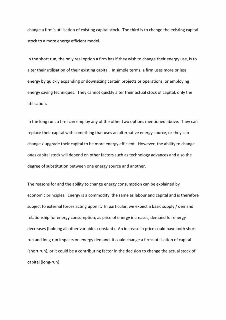
change a firm’s utilisation of existing capital stock. The third is to change the existing capital
stock to a more energy efficient model.
In the short run, the only real option a firm has if they wish to change their energy use, is to
alter their utilisation of their existing capital. In simple terms, a firm uses more or less
energy by quickly expanding or downsizing certain projects or operations, or employing
energy saving techniques. They cannot quickly alter their actual stock of capital, only the
utilisation.
In the long run, a firm can employ any of the other two options mentioned above. They can
replace their capital with something that uses an alternative energy source, or they can
change / upgrade their capital to be more energy efficient. However, the ability to change
ones capital stock will depend on other factors such as technology advances and also the
degree of substitution between one energy source and another.
The reasons for and the ability to change energy consumption can be explained by
economic principles. Energy is a commodity, the same as labour and capital and is therefore
subject to external forces acting upon it. In particular, we expect a basic supply / demand
relationship for energy consumption; as price of energy increases, demand for energy
decreases (holding all other variables constant). An increase in price could have both short
run and long run impacts on energy demand, it could change a firms utilisation of capital
(short run), or it could be a contributing factor in the decision to change the actual stock of
capital (long-run).

5
Economic research plays a very large role in the analysis of demand for energy. Over the
last forty years, there have been vast improvements in the way in which economists and
econometricians have been able to model the relationships between energy demand and
economic factors. For modelling energy consumption over time, there are currently a
number of different techniques being utilised, and the following section will present a
summary of these.
ii. Modelling Techniques
There are a vast number of approaches that have been used over the years to look into
modelling energy consumption over time. The decision on which technique to employ
depends greatly on a number of different factors, including but not limited to; availability of
data, volatility / behaviour of time series in question, as well as output requirements for the
specific project (e.g. whether short run or long run elasticity is the focus). There is also the
matter of the aggregation level of the data itself being a very important aspect to consider
when performing any sort of energy demand analysis (Bernstein & Madlener, 2010).
Level Models
The basic model, represented below has both the dependant and independent variables
logged. This allows for the direct interpretation of coefficients 2 3 and which represent
the short run elasticities of price and income respectively:
1 2 3ln( ) ln( ) ln( ).t t tE P Y (2.1)
where E, P and Y represent energy, price and output variables respectively.
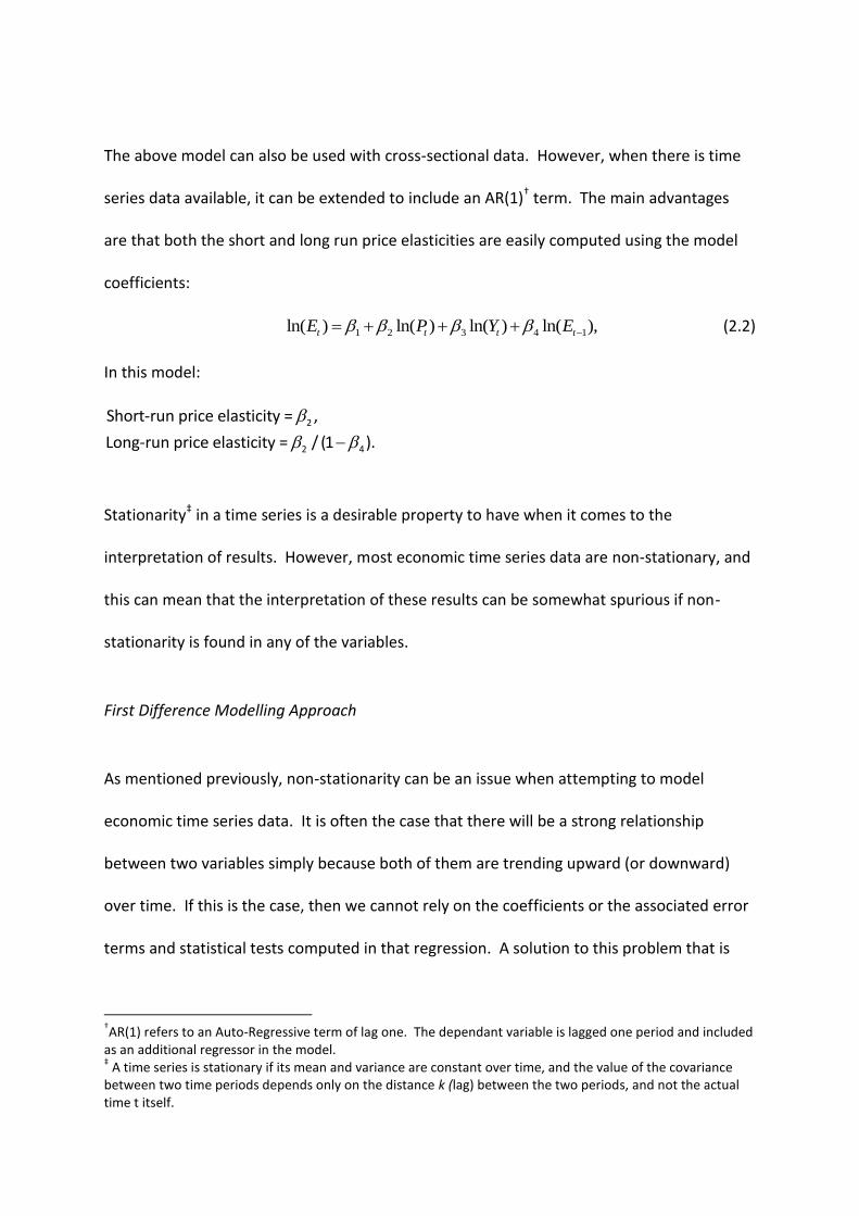
The above model can also be used with cross-sectional data. However, when there is time
series data available, it can be extended to include an AR(1)† term. The main advantages
are that both the short and long run price elasticities are easily computed using the model
coefficients:
1 2 3 4 1ln( ) ln( ) ln( ) ln( ),t t t tE P Y E (2.2)
In this model:
2
2 4
Short-run price elasticity = ,
Long-run price elasticity = / (1 ).
Stationarity‡ in a time series is a desirable property to have when it comes to the
interpretation of results. However, most economic time series data are non-stationary, and
this can mean that the interpretation of these results can be somewhat spurious if non-
stationarity is found in any of the variables.
First Difference Modelling Approach
As mentioned previously, non-stationarity can be an issue when attempting to model
economic time series data. It is often the case that there will be a strong relationship
between two variables simply because both of them are trending upward (or downward)
over time. If this is the case, then we cannot rely on the coefficients or the associated error
terms and statistical tests computed in that regression. A solution to this problem that is
†AR(1) refers to an Auto-Regressive term of lag one. The dependant variable is lagged one period and included
as an additional regressor in the model. ‡ A time series is stationary if its mean and variance are constant over time, and the value of the covariance
between two time periods depends only on the distance k (lag) between the two periods, and not the actual time t itself.
7
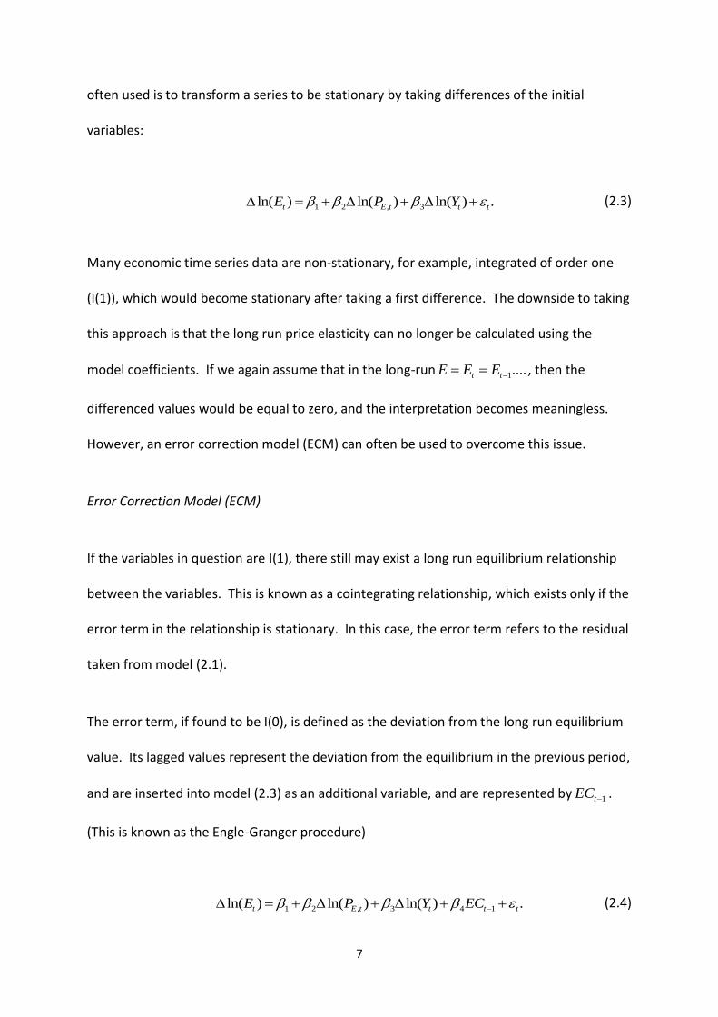
often used is to transform a series to be stationary by taking differences of the initial
variables:
1 2 , 3ln( ) ln( ) ln( ) .t E t t tE P Y (2.3)
Many economic time series data are non-stationary, for example, integrated of order one
(I(1)), which would become stationary after taking a first difference. The downside to taking
this approach is that the long run price elasticity can no longer be calculated using the
model coefficients. If we again assume that in the long-run 1....t tE E E , then the
differenced values would be equal to zero, and the interpretation becomes meaningless.
However, an error correction model (ECM) can often be used to overcome this issue.
Error Correction Model (ECM)
If the variables in question are I(1), there still may exist a long run equilibrium relationship
between the variables. This is known as a cointegrating relationship, which exists only if the
error term in the relationship is stationary. In this case, the error term refers to the residual
taken from model (2.1).
The error term, if found to be I(0), is defined as the deviation from the long run equilibrium
value. Its lagged values represent the deviation from the equilibrium in the previous period,
and are inserted into model (2.3) as an additional variable, and are represented by 1tEC .
(This is known as the Engle-Granger procedure)
1 2 , 3 4 1ln( ) ln( ) ln( ) .t E t t t tE P Y EC (2.4)

Coefficients 2 3and still represent the short run price and income elasticities, and 4
would represent the “speed of adjustment to equilibrium values” (Ryan and Plourde, 2009).
For example, a 4 value of -0.7 would mean that deviations from the equilibrium are
corrected at approximately 70 per cent per time period, t.
Other Models
In recent years, there were also other modelling approaches, for example, Vector Error
Correction Model (when more than one cointegrating relationship are found) or panel
VECM when there are panel datasets available. However, given the short time series of the
data used in this study, and also given that the above mentioned models require heavy
parameterisation, we did not pursue these models. Further explanation on our preferred
model is provided below.
iii. Modelling approach utilised in this study
For this study, based on an examination of the available data and the alternative modelling
approaches, the ECM method was considered the most appropriate for deriving short run
elasticities for electricity and natural gas consumption.
Testing for stationarity proved that most variables in question were in fact non-stationary,
and typically I(1) processes (see Table A2, Appendix), as is expected from economic variables
of this nature. As a result, the level models were ruled out due to their interpretability
being questionable and the possible spurious nature of the associated test statistics.

9
III. Data
i. Energy Data - Australian Energy Statistics (ABARES / BREE Table F)
BREE releases a yearly publication called “Australian Energy Statistics” (AES). Energy
consumption, by industry and fuel type, are provided in Table F of this publication (BREE,
2012). Up until 2011, these data were produced by the Australian Bureau of Agriculture and
Resource Economics and Sciences (ABARES) and published in the ‘Energy in Australia’ yearly
release. The data spans back to the 1973-74 financial year, providing 37 years of time series
data at each sub level. Energy consumption is broken into three separate components: fuels
consumed, derived fuels produced and net energy consumption. Fuels consumed data are
used in this study.
ii. Price and Income Data
ABS PPI Data - Electricity and Natural Gas
The ABS collects and publishes price data for a range of different energy types. For this
study, we utilise the ABS Producer Price Index (PPI) series, which is released quarterly (cat.
no. 6427.0). Tables 13 and 14 of this publication provide price indices for electricity and gas
used in the manufacturing industry. These indices are produced quarterly and date back to
1970. It is from these tables that the electricity and gas prices were taken. Due to energy
consumption being financial year data, an average of the corresponding four quarters of
price index data was taken to derive the financial year average price.
Gross Value Added (GVA) data

The ABS National Accounts Branch (NAB) releases a yearly publication ‘National Income,
Expenditure and Product’ (cat. no. 5206.0). Table 33 of this publication includes the
Industry gross value added (GVA) chain volume measures (CVM) for each industry. For the
purpose of this investigation the GVA for the Manufacturing industry has been used as our
measure of income. The data for the Manufacturing industry dates back to 1975.
Due to BREE data not fully available at the sub-sector level and with ABS PPI data only
available for manufacturing division and only for electricity and gas over the study period,
our analysis is mainly focused on the consumption of these fuels in manufacturing industry.
The following graphs show the data series in log form. All series demonstrate a global
upward trend. Apart from price series, electricity and value added series show a significant
dip after the global financial crisis in 2008-09.

11
Figure1. Time Series Data
Note: All variables presented are in log form. LELEC, LNAT_GAS, LELEC_PRICE, LNAT_GAS_PRICE and LGVA are electricity consumption, natural gas consumption, electricity price, natural gas price and gross value added respectively.
4.4
4.8
5.2
5.6
6.0
1975 1980 1985 1990 1995 2000 2005
LELEC
4.4
4.8
5.2
5.6
6.0
6.4
1975 1980 1985 1990 1995 2000 2005
LNAT_GAS
3.2
3.6
4.0
4.4
4.8
5.2
1975 1980 1985 1990 1995 2000 2005
LELEC_PRICE
3.2
3.6
4.0
4.4
4.8
5.2
1975 1980 1985 1990 1995 2000 2005
LNAT_GAS_PRICE
11.1
11.2
11.3
11.4
11.5
11.6
11.7
1975 1980 1985 1990 1995 2000 2005
LGVA

IV. Results
i. Cointegration and Stationarity Tests
It was decided that an ECM approach was appropriate after results of stationarity and
cointegration tests were completed. As explained in Section 2, a cointegrating relationship
represents the long run or equilibrium relationship between the variables in question
(Plourde and Ryan, 2009). We conducted Augmented Dickey Fuller (ADF) test for all
variables. Results suggested they are non-stationary - I(1).
The tables below show the results of the test for cointegration between the explanatory
variables for the consumption of electricity:
Table 1. Level Model regression - dependant variable: Log electricity consumption
Note: C, LELEC_PRICE, LGVA and LNAT_GAS_PRICE are the intercept and log of electricity price, gross value added and natural gas price respectively.

13
Whilst the variables are I(1), ADF test shows the model residuals are I(0) (i.e. stationary, as
the null hypothesis for a unit root is rejected), implying that a long run cointegrating
relationship exists between the variables in question.
Table 2. Augmented Dickey Fuller test
Note: RESID_ELEC1_3 is estimate of residual from the model in Table 1.
ii. Model Specification
Below is the specification for the final ECM models used in this paper. As mentioned
previously, data limitations constrained the analysis to only two different fuel types;
electricity and natural gas. A two stage Engle-Granger approach was used to formulate the
ECM models; the two cointegrating relationships used are:
0 1 , 2 3 , ,ln( ) ln( ) ln( ) ln( )t E t t G t E tE P Y P , (4.1)
and
0 1 , 2 3 , ,ln( ) ln( ) ln( ) ln( )t G t t E t G tG P Y P . (4.2)

The cointegrating relationships above represent the long run equilibrium for the two fuel
types, and the residuals from these relationships represent the deviation from the
equilibrium. The residuals from model (4.1) and (4.2) were lagged and included in the ECM
models for electricity and gas consumption respectively. The specification for the error
correction models are below:
0 1 , 2 3 , 4 1 5 6ln( ) ln( ) ln( ) ln( )t E t t G t t tE P Y P EC GFC T ,(4.3)
and
0 1 , 2 3 , 4 1 5 6ln( ) ln( ) ln( ) ln( )t G t t E t t tG P Y P EC GFC T ,(4.4)
where:
tE is the Electricity consumption at time t,
Gt is the Natural Gas consumption at time t,
,E tP is the price of Electricity at time t,
tY is the measure of Income (GVA) for the manufacturing industry at time t,
,G tP is the price of Natural Gas at time t,
1tEC is the error correction component for time t-1 taken from equations (4.1) and (4.2),
GFC is a dummy variable representing the time period before and after the GFC and,
T is a time trend.
15
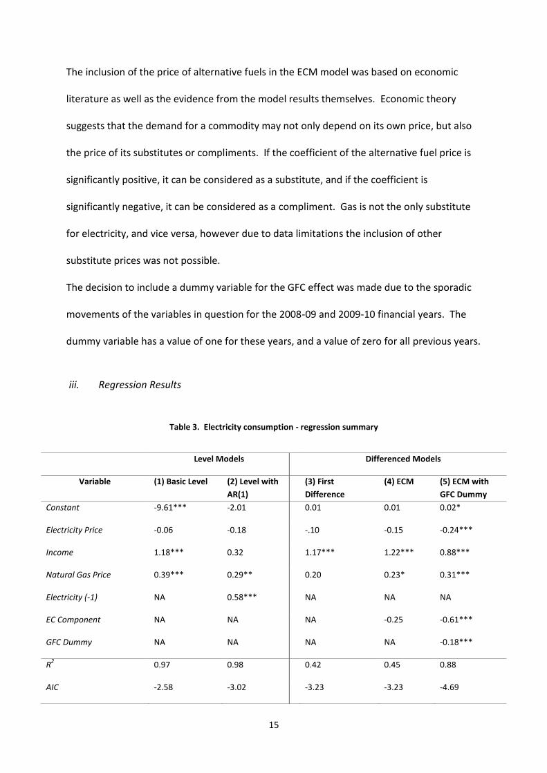
The inclusion of the price of alternative fuels in the ECM model was based on economic
literature as well as the evidence from the model results themselves. Economic theory
suggests that the demand for a commodity may not only depend on its own price, but also
the price of its substitutes or compliments. If the coefficient of the alternative fuel price is
significantly positive, it can be considered as a substitute, and if the coefficient is
significantly negative, it can be considered as a compliment. Gas is not the only substitute
for electricity, and vice versa, however due to data limitations the inclusion of other
substitute prices was not possible.
The decision to include a dummy variable for the GFC effect was made due to the sporadic
movements of the variables in question for the 2008-09 and 2009-10 financial years. The
dummy variable has a value of one for these years, and a value of zero for all previous years.
iii. Regression Results
Table 3. Electricity consumption - regression summary
Level Models Differenced Models
Variable (1) Basic Level (2) Level with
AR(1)
(3) First
Difference
(4) ECM (5) ECM with
GFC Dummy
Constant -9.61*** -2.01 0.01 0.01 0.02*
Electricity Price -0.06 -0.18 -.10 -0.15 -0.24***
Income 1.18*** 0.32 1.17*** 1.22*** 0.88***
Natural Gas Price 0.39*** 0.29** 0.20 0.23* 0.31***
Electricity (-1) NA 0.58*** NA NA NA
EC Component NA NA NA -0.25 -0.61***
GFC Dummy NA NA NA NA -0.18***
R2
0.97 0.98 0.42 0.45 0.88
AIC -2.58 -3.02 -3.23 -3.23 -4.69
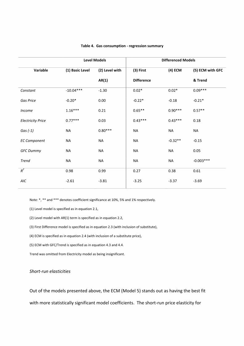
Table 4. Gas consumption - regression summary
Level Models Differenced Models
Variable (1) Basic Level (2) Level with
AR(1)
(3) First
Difference
(4) ECM (5) ECM with GFC
& Trend
Constant -10.04*** -1.30 0.02* 0.02* 0.09***
Gas Price -0.20* 0.00 -0.22* -0.18 -0.21*
Income 1.16*** 0.21 0.65** 0.90*** 0.57**
Electricity Price 0.77*** 0.03 0.43*** 0.43*** 0.18
Gas (-1) NA 0.80*** NA NA NA
EC Component NA NA NA -0.32** -0.15
GFC Dummy NA NA NA NA 0.05
Trend NA NA NA NA -0.003***
R2
0.98 0.99 0.27 0.38 0.61
AIC -2.61 -3.81 -3.25 -3.37 -3.69
Note: *, ** and *** denotes coefficient significance at 10%, 5% and 1% respectively.
(1) Level model is specified as in equation 2.1,
(2) Level model with AR(1) term is specified as in equation 2.2,
(3) First Difference model is specified as in equation 2.3 (with inclusion of substitute),
(4) ECM is specified as in equation 2.4 (with inclusion of a substitute price),
(5) ECM with GFC/Trend is specified as in equation 4.3 and 4.4.
Trend was omitted from Electricity model as being insignificant.
Short-run elasticities
Out of the models presented above, the ECM (Model 5) stands out as having the best fit
with more statistically significant model coefficients. The short-run price elasticity for

17
electricity derived from this model is -0.24 (a 1 per cent increase in the price of electricity
leads to 0.24 per cent decrease in the demand for electricity, holding other variables
constant). This value is consistent with Bernstein and Griffin’s 2005 results, in which they
found the short-run commercial price elasticity for USA to be -0.21.
It is important to note that this study uses aggregated data, and as explained by Steinbuks
(2010), there are possible associated biases that arise due to the nature of the data. For
example, aggregate data fails to account for the large differences in technological
requirements in specific industries. The substitution observed from model results could be
due to merely firm entry and exit. An elasticity of -0.24 is on the high end of the values
typically found, and this could include some upward bias in the estimate.
As expected there is a significant positive relationship between income (GVA) and the
demand for electricity, with a short run income elasticity of 0.88. Again, this value is within
the range typically found for income elasticities.
Short-run price elasticity for gas consumption is found to be -0.21 (Model 5, Table 4).
Long run equilibrium relationship
Whilst the Engle and Granger ECM model does not allow the interpretation of individual
long run elasticities, it can provide an indication of the speed at which the energy demand
reverts back to its long run equilibrium. As mentioned previously, if we assume that
1....t tE E E is the long run equilibrium demand, then the error correction term
provides information on the deviation from this equilibrium.

For the consumption of electricity, the Error Correction (EC) term is -0.61, which suggests
that deviations from the long run equilibrium are corrected at a rate of approximately 61
per cent per year. The coefficient for the EC term in the gas model is not found to be
significant; however the coefficient for the trend variable is statistically significant.
V. Conclusion
This study provides an investigation into the electricity and gas consumption by the
Australian manufacturing industry. More specifically, it looks into the associated price
elasticities of demand for these energy sources. Whilst there have been many papers
written that investigate energy consumption at industry levels, there are few papers that
use Australian energy data.
The methodological technique and selection of regression models is based largely on the
findings of European and American papers. This report investigates the pros and cons of
several energy modelling techniques, with the focus being on the Error Correction Model.
The data used has been sourced from the Bureau of Resources and Energy Economics, as
well as the Australian Bureau of Statistics. This analysis is based on yearly data ranging from
1973 to 2010.
The study has found statistically significant relationships between the dependant variables
(electricity and natural gas consumption), and the explanatory variables in question. Short
run price elasticity for electricity and gas consumption was found to be -0.24 and -0.21
respectively. Both these values were within the range of price elasticities found in other
investigations of this nature.

19
A summary of the elasticity estimates is provided in the table below.
Table 5. Summary of estimates
Variable (1) Basic Level (2) Level
with AR(1)
(3) First
Difference
(4) ECM (5) ECM with
GFC Dummy
Electricity Consumption
Electricity Price -0.06 -0.18 -.10 -0.15 -0.24***
Natural Gas Price 0.39*** 0.29** 0.20 0.23* 0.31***
Electricity (-1) NA 0.58*** NA NA NA
EC Component NA NA NA -0.25 -0.61***
Gas Consumption
Gas Price -0.20* 0.00 -0.22* -0.18 -0.21*
Electricity Price 0.77*** 0.03 0.43*** 0.43*** 0.18
Gas (-1) NA 0.80*** NA NA NA
EC Component NA NA NA -0.32** -0.15
Note: The coefficients of electricity price (in electricity consumption equation) and gas price (in gas
consumption equation) give the short run elasticity estimates. Long run adjustments are implied by the
estimates of either the coefficient of the lag price variable (in AR(1) model) or the coefficient of the EC
component.
There are other alternative approaches that have not been investigated in this study. The
use of VAR and VECM techniques can provide further valuable information regarding long-
run price elasticities as well as the causal nature of the data. Further research of this nature
will be considered in an extension to this project.

REFERENCES
Akmal, M., and Stern, D. (2001), ‘Residential Energy Demand in Australia: An Application
of Dynamic OLS’, Centre for Resource and Environmental Studies, Australian
National University (ANU).
Belke, A., Dreger, C. and de Haan, F. (2010), ‘Energy Consumption and Economic Growth:
New Insights into the Cointegration Relationship’, Ruhr Economic Papers #190,
Ruhr-Universität Bochum (RUB), Germany.
Bernstein, R. and Madlener, R. (2010), ‘Short- and Long-Run Electricity Demand
Elasticities at the Subsectoral Level: A Cointegration Analysis for German
Manufacturing Industries’, E.ON Energy Research Center, RWTH Aachen
University, Germany.
Best, R. (2008), ‘An Introduction to Error Correction Models’, Oxford Spring School for
Quantitative Methods in Social Research.
BREE, (2012), Australian Energy Statistics. Available at
http://www.bree.gov.au/publications/aes-2012.html
Cao, K., Wong, J. and Kumar, A. (2012), “Modelling the National Greenhouse and Energy
Reporting System (NGER) energy consumption under-coverage”, Australian
Bureau of Statistics (ABS) research paper, available at
http://www.abs.gov.au/ausstats/[email protected]/mf/1351.0.55.040
Cao, K., Wong, J. and Kumar, A. (2013), “Modelling the National Greenhouse and Energy
Reporting System (NGER) energy consumption under-coverage”, Australian
Economic Review, upcoming June 2013 issue.

21
Che, N. and Pham, P. (2012), ‘Economic Analysis of End-use Energy Intensity in
Australia’, Bureau of Resources and Energy Economics (BREE) research paper.
Cooper, J. (2003), ‘Price elasticity of demand for crude oil: estimates for 23 countries’,
Department of Economics at Glasgow Caledonian University working paper.
Medlock, K. (2009), ‘Energy Demand Theory’, in J. Evans and L.C. Hunt (eds),
International Handbook on the economics of Energy, Edward Elgar, Cheltenham.
Roarty, M. (2008), ‘Australia’s natural gas: issues and trends’, Department of
Parliamentary Services (DPS).
Ryan, L. and Plourde, A. (2009), ‘Empirical modelling of energy demand’, in J. Evans and
L.C. Hunt (eds), International Handbook on the economics of Energy, Edward
Elgar, Cheltenham.
Samimi, R. (1995), ‘Road transport energy demand in Australia: A cointegration
approach’ Energy Economics, Vol. 17, No. 4, pp. 329-339.
Soytas, U., Sari, R. and Ozdemir, O. (2001), ‘Energy Consumption and GDP Relations in
Turkey: A Cointegration and Vector Error Correction Analysis’, Economies and
Business in Transition: Facilitating Competitiveness and Change in the Global
Environment Proceedings, 2001, Global Business and Technology Association, pp.
838-844.
Steinbuks, J. (2010), ‘Interfuel Substitution and Energy Use in the UK Manufacturing
Sector’, EPRG Working Paper 1015, University of Cambridge.

APPENDIXES
Table A1. Energy Consumption (PJ), Manufacturing
Energy Source Other Energy Sources
Year Electricity Gas
Refinery feedstock Coke
Petroleum products
1973-74 87.6 85.7
1 230.1 139.4 169.9
1974-75 88.4 93.1
1 231.9 148.6 167.1
1975-76 90.1 103.3
1 233.7 135.3 163.9
1976-77 94.7 117.5
1 289.8 132.6 177.5
1977-78 97.6 134.2
1 331.1 130.0 182.3
1978-79 103.3 148.8
1 320.4 141.9 168.4
1979-80 109.9 179.1
1 312.8 137.1 161.6
1980-81 115.4 198.6
1 261.7 116.3 149.4
1981-82 118.0 206.1
1 276.1 124.7 144.6
1982-83 116.5 212.5
1 235.6 96.4 129.7
1983-84 133.6 215.7
1 260.9 95.3 140.3
1984-85 147.1 245.7
1 267.5 94.9 135.6
1985-86 155.6 264.3
1 247.2 89.3 136.0
1986-87 163.7 278.5
1 233.4 86.0 138.8
1987-88 177.6 284.5
1 321.6 82.3 146.8
1988-89 190.6 291.3
1 345.7 86.0 152.1
1989-90 196.7 300.2
1 386.3 114.4 142.9
1990-91 197.7 303.7
1 421.4 113.6 153.7
1991-92 198.3 303.2
NA 97.5 150.6
1992-93 204.9 309.2
NA 95.2 162.2
1993-94 213.9 327.2
NA 104.0 164.4
1994-95 214.0 338.2
NA 107.3 172.4
1995-96 213.2 336.0
NA 106.8 178.2
1996-97 219.6 354.4
NA 106.1 157.2
1997-98 238.6 356.3
NA 102.1 169.7
1998-99 249.8 356.6
1 675.1 106.7 168.5
1999-00 259.8 368.4
1 714.0 98.5 167.2
2000-01 265.6 397.8
1 695.0 83.6 157.0
2001-02 267.4 397.5
1 667.8 81.4 154.2
2002-03 275.6 422.0
1625.6 74.5 162.0
2003-04 277.4 431.1
1527.1 80.0 190.8
2004-05 293.5 405.0
1540.7 77.1 212.7
2005-06 293.1 404.5
1406.6 76.0 203.6
2006-07 300.4 417.0
1503.1 76.7 205.9
2007-08 307.4 414.8
1462.1 78.0 205.7
2008-09 242.9 423.1
1476.3 63.0 202.1
2009-10 240.9 439.1 1434.1 72.9 194.4
Source: Energy in Australia 2011, BREE.

23
Table A2. Augmented Dickey Fuller Tests Results
ADF Test
Variable Lag 1 Coefficient
Durbin Watson
P-Value Unit root
Original Series
Electricity Consumption -0.06** 1.77 0.1105 Yes
Natural Gas Consumption -0.10*** 1.86 0.0000 No*
Electricity Price -0.08*** 1.16 0.0218 No*
Natural Gas Price -0.03* 1.88 0.3894 Yes
Gross Value Added (GVA) -0.04 1.86 0.6833 Yes
1st Difference
Electricity Consumption -0.79*** 1.99 0.0012 No
Natural Gas Consumption -0.50*** 2.19 0.0172 No
Electricity Price -0.47*** 2.06 0.0383 No
Natural Gas Price -0.38*** 1.82 0.0730 No
Gross Value Added (GVA)
-0.93*** 1.93 0.0002 No
Note: The ADF tests for the Null hypothesis of having a unit root. Therefore when the P-value is smaller than
the critical value (0.05), the Null is rejected and the conclusion is no unit root or the series is stationary - I(0). In
a few cases (e.g. natural gas consumption and electricity price), although ADF test shows no strong evidence of
unit root, the diagnostics through Correlogram and other tests still suggest some evidence of non-stationarity.
For this reason, most of original series in this study are deemed non-stationary – I(1) while the first difference
series are stationary – I(0).