Embed Size (px)
Citation preview
J Sci Comput (2014) 59:721–759DOI 10.1007/s10915-013-9780-2
Energy Stable Flux Reconstruction Schemesfor Advection–Diffusion Problems on Tetrahedra
D. M. Williams · A. Jameson
Received: 16 April 2013 / Revised: 1 August 2013 / Accepted: 30 August 2013 /Published online: 24 September 2013© Springer Science+Business Media New York 2013
Abstract The flux reconstruction (FR) methodology provides a unifying description of manyhigh-order schemes, including a particular discontinuous Galerkin (DG) scheme and severalspectral difference (SD) schemes. In addition, the FR methodology has been used to gen-erate new classes of high-order schemes, including the recently discovered ‘energy stable’FR schemes. These schemes, which are often referred to as VCJH (Vincent–Castonguay–Jameson–Huynh) schemes, are provably stable for linear advection–diffusion problems in 1Dand on triangular elements. The VCJH schemes have been successfully applied to a wide vari-ety of problems in 1D and 2D, ranging from linear advection–diffusion problems, to fluidmechanics problems requiring the solution of the compressible Navier–Stokes equations.Based on the results of these numerical experiments, it has been shown that certain VCJHschemes maintain the expected order of spatial accuracy and possess explicit time-step limitswhich rival those of the collocation-based nodal DG scheme. However, it remained to beseen whether the VCJH schemes could be extended to 3D on tetrahedral elements, enablingtheir convenient application to the complex geometries that arise in many real-world prob-lems. For the first time, this article presents an extension of the VCJH schemes to tetrahedralelements. This work provides a formal proof of the stability of the new schemes and assessestheir performance via numerical experiments on model problems.
Keywords High-order · Unstructured · Discontinuous Galerkin · Spectral difference ·Flux reconstruction · Tetrahedra
Mathematics Subject Classification (2000) 65M12 · 65M60 · 65M70 · 35Q35 · 35L65 ·35Q30
D. M. Williams (B) · A. JamesonStanford University, Stanford, CA 94305, USAe-mail: [email protected]
123
722 J Sci Comput (2014) 59:721–759
1 Introduction
It is generally believed that higher fidelity numerical methods are needed for solving manyof the unsteady, compressible, viscous flow problems that arise in industrial settings. Cur-rently, such problems are frequently solved using second-order methods on unstructuredmeshes of triangular and tetrahedral elements [20]. However, these second-order methodsintroduce numerical dissipation that interferes with the propagation of vortices and othertime-dependent phenomena. As a result, there has been significant interest in developinghigh-order methods that are suitable for unstructured meshes (cf. the recent review articleby Vincent and Jameson [34]). These high-order methods have the potential to produce lessdissipation and to obtain more accurate results at lower computational cost [19]. However,these methods appear to be less robust and more difficult to implement than their low-ordercounterparts, and therefore, despite their promise, have yet to be adopted by the majority offluid dynamicists.
In order to address this issue, there have been efforts to improve the flexibility and easeof implementation of high-order methods, and in particular the well-known discontinuousGalerkin (DG) methods. These efforts have brought about a rise in popularity of ‘nodal’ DGmethods that omit the explicit use of quadratures (as described in [19]), allowing them to serveas simpler alternatives to the classical DG methods that utilize complex quadrature procedures(described in [3,4,11]). There have also been efforts to develop an alternative class of high-order methods referred to as spectral difference (SD) methods. The SD methods, originallyproposed by Kopriva and Kolias [27] and generalized by Liu, Vinokur, and Wang [29], omitthe explicit use of quadratures by employing a nodal representation of the solution, wherethe nodes are placed at the locations of the Chebyshev points. Finally, there have been effortsto develop the flux reconstruction (FR) methodology (discovered by Huynh [22]) whichprovides a unifying framework for a number of well-known nodal DG and SD schemes, andestablishes an intuitive methodology for identifying new classes of robust high-order schemes.In particular, Huynh has used the FR methodology to identify new high-order schemes foradvection and diffusion problems in 1D [22,23] and in 2D [23,24] on quadrilateral andtriangular elements. In addition, Wang, Gao, Haga, and Yu have identified new schemes,referred to as correction procedure via reconstruction (CPR) schemes [18,39], which are ageneralization of the FR schemes and the (closely related) lifting collocation penalty (LCP)schemes [15,17,35,36]. The CPR schemes have been successfully applied to a wide range ofproblems in 2D on quadrilateral and triangular elements [15,35,36] and in 3D on prismaticand tetrahedral elements [17,18]. The reader may consult [38] for a more comprehensivereview of the CPR approach along with other FR (and FR-type) approaches.
As the discussion above indicates, there are many FR schemes to choose from. However,it is preferable to consider only those schemes whose stability can be rigorously established.Towards this end, Huynh has employed Fourier analysis [22,23], and Wang, Gao, Haga,and Yu have employed numerical experiments [15,17,18,35,36] in order to establish thestability of their respective classes of FR schemes. Alternatively, Jameson [25], Vincentet al. [33], Castonguay et al. [9,10], and Williams et al. [38] have employed an ‘energystability’ approach to identify a particular class of stable FR schemes. This approach is moregeneral than that of Fourier analysis and numerical experimentation, as it produces resultswhich hold for all orders of accuracy on arbitrary unstructured grids. In [25], Jameson usedthis approach to identify a particular SD scheme that is provably stable for linear advectionproblems in 1D. Thereafter, Vincent et al. [33] extended this approach to identify an infiniterange of ‘energy stable’ FR schemes that are provably stable for linear advection problems in1D. These schemes, referred to as Vincent–Castonguay–Jameson–Huynh (VCJH) schemes,
123
J Sci Comput (2014) 59:721–759 723
are parameterized by a single scalar c, and for an appropriate choice of this scalar, onecan recover a collocation-based nodal DG scheme along with the SD scheme that Jamesonidentified in [25]. Most recently, Castonguay et al. [9,10] and Williams et al. [38] used theenergy stability approach to identify a class of FR schemes that are provably stable for linearadvection–diffusion problems in 1D and on triangular elements. These schemes (also referredto as VCJH schemes) are parameterized by two scalars c and κ , and for appropriate choices ofthese scalars, it can be shown that a collocation-based nodal DG scheme is recovered. In [38],the resulting schemes were successfully applied to linear and nonlinear advection–diffusionproblems in 2D, and it was shown that certain VCJH schemes maintain the expected order ofspatial accuracy while possessing explicit time-step limits that are more than 2x larger thanthose of the collocation-based nodal DG scheme.
To the authors’ knowledge, a class of energy stable FR schemes has yet to be developedfor advection–diffusion problems on tetrahedral elements. In this work, the FR approach thatwas proven to be stable for linear advection–diffusion problems on triangular elements in[9,10], and [38], will be extended to tetrahedral elements. This will result in a new class ofhigh-order methods for unstructured meshes of tetrahedral elements.
The remainder of this article has the following structure. Section 2 describes the general FRapproach for treating tetrahedral elements. Section 3 introduces the energy stable FR approach(i.e. the VCJH approach) for tetrahedral elements and proves the stability of this approach forlinear advection–diffusion problems. Section 4 identifies values of the coefficients c and κthat preserve the spatial symmetry of the schemes. Section 5 proves that the resulting class ofVCJH schemes is equivalent to a class of filtered DG schemes. Section 6 presents the VCJHschemes which have explicit time-step limits that are maximal (for linear advection problems).Finally, in an effort to further assess the capabilities of the VCJH schemes, section 7 presentsthe results of numerical experiments on a canonical linear advection–diffusion problem.
2 Flux Reconstruction for Advection–Diffusion Problems on Tetrahedral Elements
In what follows, the general FR methodology for advection–diffusion problems on triangularelements, described by Castonguay et al. [9,10] and Williams et al. [38], is extended totetrahedral elements.
2.1 Preliminaries
Consider the 3D advection–diffusion equation which (in accordance with [5]) can beexpressed as the following first-order system
∂u
∂t+ ∇ · f = 0, (1)
q − ∇u = 0, (2)
where u is a scalar solution, t is time, ∇ is the gradient operator defined such that
∇ ≡(∂∂x ,
∂∂y ,
∂∂z
), x = (x, y, z) = (x1, x2, x3) are spatial coordinates, f = f (u,q) is
an advective-diffusive flux, and q is an ‘auxiliary variable.’ One seeks a solution to the sys-tem given by Eqs. (1) and (2) within the 3D domain � with boundary �. Towards this end,the domain can be divided into N conforming, non-overlapping, straight-sided tetrahedralelements �k (where k = 1, . . . , N ), and within each element the solution u can be approxi-mated by a function u D
k which is continuously defined within �k and which vanishes outside
123
724 J Sci Comput (2014) 59:721–759
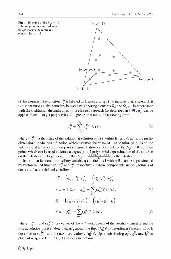
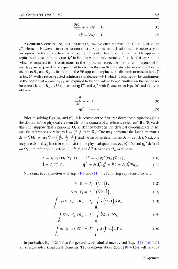
Fig. 1 Example of the Np = 10solution point locations (denotedby spheres) in the referenceelement for p = 2
(−1,1,−1)
(1,−1,−1)
(−1,−1,−1)
(−1,−1,1)
of the element. The function u Dk is labeled with a superscript D to indicate that, in general, it
is discontinuous at the boundary between neighboring elements �k and �k+1. In accordancewith the traditional, discontinuous finite element approach (as described in [19]), u D
k can beapproximated using a polynomial of degree p that takes the following form
u Dk =
Np∑i=1
(u Dk )
i �i (x) , (3)
where (u Dk )
i is the value of the solution at solution point i within �k and �i (x) is the multi-dimensional nodal basis function which assumes the value of 1 at solution point i and thevalue of 0 at all other solution points. Figure 1 shows an example of the Np = 10 solutionpoints which can be used to define a degree p = 2 polynomial approximation of the solutionon the tetrahedron. In general, note that Np = (p+1)(p+2)(p+3)
6 on the tetrahedron.In a similar fashion, the auxiliary variable q and the flux f within �k can be approximated
by vector-valued functions qDk and f D
k (respectively) whose components are polynomials ofdegree p that are defined as follows
qDk =
(q D
xk, q D
yk, q D
zk
)=(
q D1k, q D
2k, q D
3k
),
∀ m = 1, 2, 3, q Dmk
=Np∑i=1
(q Dmk)i �i (x) , (4)
f Dk =
(f Dxk, f D
yk, f D
zk
)=(
f D1k, f D
2k, f D
3k
),
∀ m, f Dmk
=Np∑i=1
( f Dmk)i �i (x) , (5)
where (q Dmk)i and ( f D
mk)i are values of the mth components of the auxiliary variable and the
flux at solution point i . Note that, in general, the flux ( f Dmk)i is a nonlinear function of both
the solution (u Dk )
i and the auxiliary variable (qDk )
i . Upon substituting u Dk ,qD
k , and f Dk in
place of u,q, and f in Eqs. (1) and (2), one obtains
123
J Sci Comput (2014) 59:721–759 725
∂u Dk
∂t+ ∇ · f D
k = 0, (6)
qDk − ∇u D
k = 0. (7)
As currently constructed, Eqs. (6) and (7) involve only information that is local to thekth element. However, in order to construct a valid numerical scheme, it is necessary toincorporate information from neighboring elements. Towards this end, the FR approachreplaces the discontinuous flux f D
k in Eq. (6) with a ‘reconstructed flux’ fk of degree p + 1which is required to be continuous in the following sense: the normal components of fk
and fk+1 are required to be equivalent to one another on the boundary between neighboringelements �k and �k+1. In addition, the FR approach replaces the discontinuous solution u D
kin Eq. (7) with a reconstructed solution uk of degree p +1 which is required to be continuousin the sense that uk and uk+1 are required to be equivalent to one another on the boundarybetween �k and �k+1. Upon replacing f D
k and u Dk with fk and uk in Eqs. (6) and (7), one
obtains
∂u Dk
∂t+ ∇ · fk = 0, (8)
qDk − ∇uk = 0. (9)
Prior to solving Eqs. (8) and (9), it is convenient to first transform these equations fromthe domain of the physical element �k to the domain of a ‘reference element’ �S . Towardsthis end, suppose that a mapping �k is defined between the physical coordinates x in �k
and the reference coordinates x = (x, y, z) in �S . One may construct the Jacobian matrix
Jk = ∇�k (where ∇ =(∂∂ x ,
∂∂ y ,
∂∂ z
)) and the Jacobian determinant Jk = det(Jk). Next, one
may use Jk and Jk in order to transform the physical quantities uk, u Dk , fk , and qD
k defined
on �k into reference quantities u, u D, f , and qD defined on �S as follows
u = Jk uk(�k
(x), t), u D = Jk u D
k
(�k
(x), t), (10)
f = Jk J−1k fk, qD = Jk JT
k qDk = ∇u = Jk JT
k ∇uk . (11)
Note that, in conjunction with Eqs. (10) and (11), the following equations also hold
∇ · fk = J−1k
(∇ · f
), (12)
∇uk · fk = J−2k
(∇u · f
), (13)
∫
�k
uk (∇ · fk) d�k = J−1k
∫
�S
u(∇ · f
)d�S, (14)
∫
�k
∇uk · fk d�k = J−1k
∫
�S
∇u · f d�S, (15)
∫
�k
uk (fk · n) d�k = J−1k
∫
�S
u(
f · n)
d�S . (16)
In particular, Eq. (12) holds for general tetrahedral elements, and Eqs. (13)–(16) holdfor straight-sided tetrahedral elements. The equations above (Eqs. (10)–(16)) will be used
123
726 J Sci Comput (2014) 59:721–759
frequently in subsequent discussions. For now, consider substituting Eqs. (10)–(12) intoEqs. (8) and (9), in order to obtain the following
∂ u D
∂t+ ∇ · f = 0, (17)
qD − ∇u = 0. (18)
In what follows, the FR procedure for solving Eqs. (17) and (18) will be discussed.
2.2 The FR Procedure
The FR procedure for solving Eqs. (17) and (18) involves obtaining the unknown quantities
qD , the auxiliary variable in reference space, and ∂ u D
∂t , the time rate of change of the solution
in reference space, from computations of (respectively) ∇u, the gradient of the reconstructedsolution in reference space, and ∇ · f , the divergence of the reconstructed flux in referencespace.
2.2.1 Computing ∇u, the Gradient of the Reconstructed Solution in Reference Space
In order to facilitate the computation of ∇u, one must first formulate a more precise definitionfor u. Towards this end, the FR approach requires u to take the following form on the elementboundary �S
u
∣∣∣∣�S
= u�∣∣∣∣�S
=(
u D + uC) ∣∣∣∣
�S
, (19)
where uC is a ‘solution correction’ that corrects u D in such a way that the sum of u D anduC assumes the value of u�, the value of the common numerical solution in reference space.Equation (19) ensures that u (and thus uk) is continuous at the boundary between neighboringelements �k and �k+1. In practice, Eq. (19) is enforced pointwise at the l = 1, . . . , N f p
‘flux points’ on the f = 1, . . . , Nef faces of the element, as follows
u f,l = u�f,l = u Df,l + uC
f,l ∀ f, l (20)
where (for example) u Df,l is the value of u D at flux point l on face f .
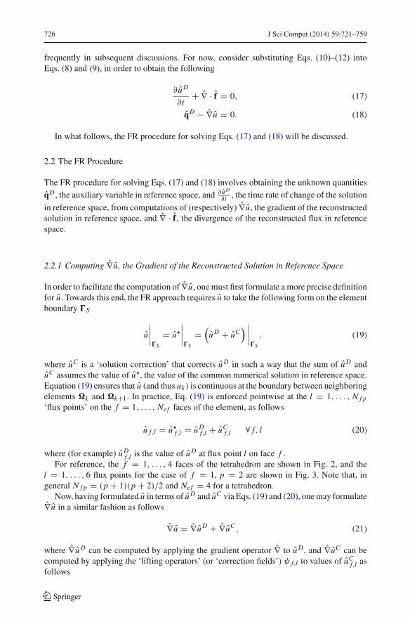
For reference, the f = 1, . . . , 4 faces of the tetrahedron are shown in Fig. 2, and thel = 1, . . . , 6 flux points for the case of f = 1, p = 2 are shown in Fig. 3. Note that, ingeneral N f p = (p + 1)(p + 2)/2 and Nef = 4 for a tetrahedron.
Now, having formulated u in terms of u D and uC via Eqs. (19) and (20), one may formulate∇u in a similar fashion as follows
∇u = ∇u D + ∇uC , (21)
where ∇u D can be computed by applying the gradient operator ∇ to u D , and ∇uC can becomputed by applying the ‘lifting operators’ (or ‘correction fields’) ψ f,l to values of uC
f,l asfollows
123
J Sci Comput (2014) 59:721–759 727
f = 2 (back)
f = 1 (front)
f = 4 (bottom)
f = 3 (back)
Fig. 2 Example of the numbering convention for the faces on the reference element
Fig. 3 Example of thenumbering convention for theflux points on the referenceelement for p = 2. The fluxpoints (denoted by squares) areshown for the face f = 1
l = 3
l = 5
l = 2
l = 6
l = 4
l = 1
∇uC (x) =N f e∑f =1
N f p∑l=1
uCf,l n f,l ψ f,l
(x)
=N f e∑f =1
N f p∑l=1
[u�f,l − u D
f,l
]n f,l ψ f,l
(x). (22)
The lifting operators ψ f,l(x) are designed to ‘lift’ (or transform) values of uC defined on�S into values of ∇uC defined on �S . In order to ensure that the operators perform this task,they are defined such that ψ f,l ≡ ∇ · g f,l , where each g f,l is a vector-valued ‘correctionfunction’ associated with flux point l on face f . In addition, the normal component of eachcorrection function (g f,l · n) is required to satisfy the following condition
123
728 J Sci Comput (2014) 59:721–759
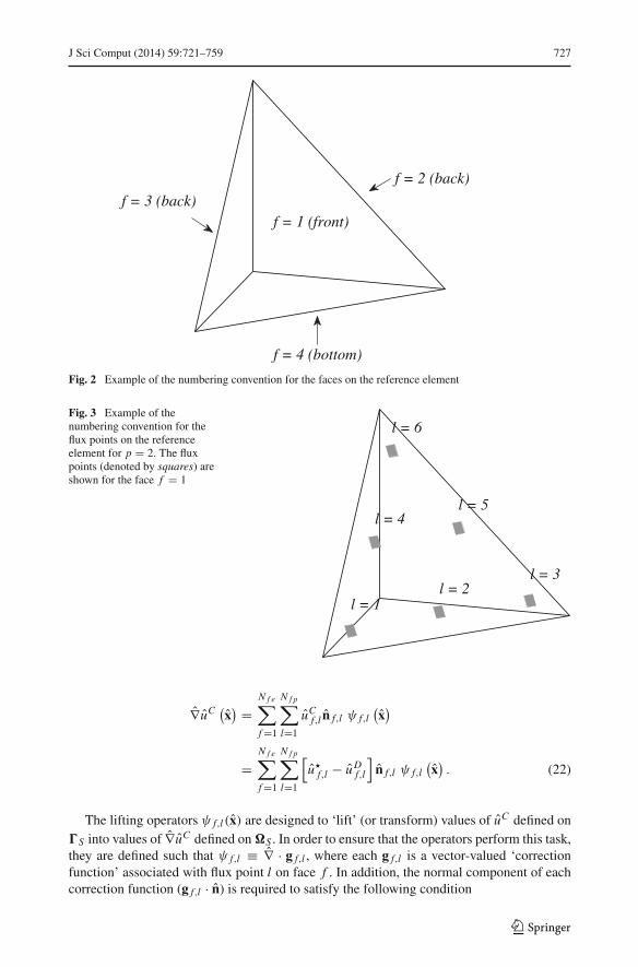
Fig. 4 Example of a vectorcorrection function g f,lassociated with flux pointf = 1, l = 2 for p = 2
Fig. 5 Contours of a correctionfield ψ f,l (where ψ f,l ≡ ∇ · g f,l )associated with flux pointf = 1, l = 2 for p = 2
g f,l(xv,w
) · nv,w ={
1 if v = f and w = l
0 if v �= f or w �= l. (23)
Furthermore, g f,l(x)
is required to belong to the Raviart–Thomas space of degree p(defined in [31]) in order to ensure that the following holds
ψ f,l ≡ ∇ · g f,l ∈ Pp (�S) , g f,l · n ∈ Rp (�S) , (24)
where Pp (�S) and Rp (�S) are spaces which contain the polynomials of degree ≤ p on �S
and �S , respectively. In [38], Williams et al. showed that Eqs. (23) and (24) ensure that ψ f,l
serves as a lifting operator that transforms uC defined on �S into ∇uC defined on �S .
123
J Sci Comput (2014) 59:721–759 729
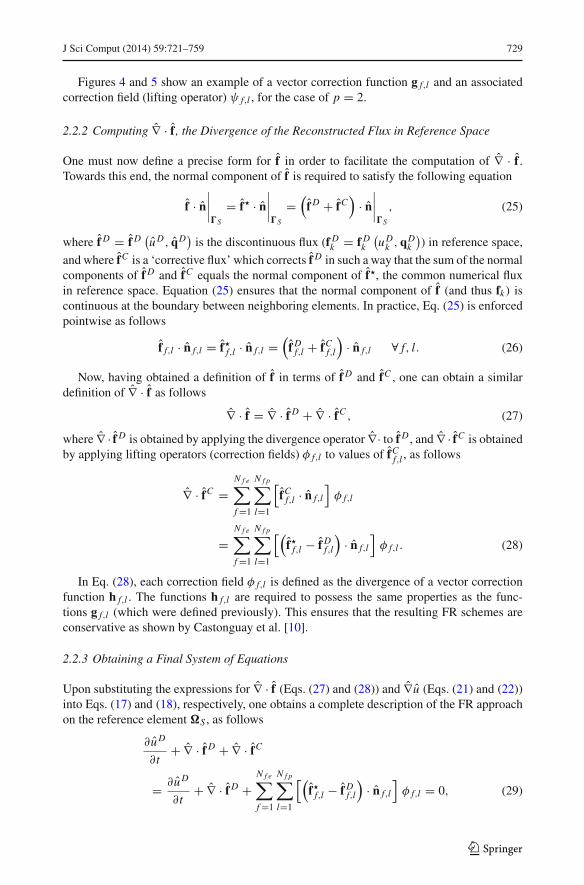
Figures 4 and 5 show an example of a vector correction function g f,l and an associatedcorrection field (lifting operator) ψ f,l , for the case of p = 2.
2.2.2 Computing ∇ · f , the Divergence of the Reconstructed Flux in Reference Space
One must now define a precise form for f in order to facilitate the computation of ∇ · f .Towards this end, the normal component of f is required to satisfy the following equation
f · n
∣∣∣∣�S
= f� · n
∣∣∣∣�S
=(
f D + fC)
· n
∣∣∣∣�S
, (25)
where f D = f D(u D, qD
)is the discontinuous flux (f D
k = f Dk
(u D
k ,qDk
)) in reference space,
and where fC is a ‘corrective flux’ which corrects f D in such a way that the sum of the normalcomponents of f D and fC equals the normal component of f�, the common numerical fluxin reference space. Equation (25) ensures that the normal component of f (and thus fk) iscontinuous at the boundary between neighboring elements. In practice, Eq. (25) is enforcedpointwise as follows
f f,l · n f,l = f�f,l · n f,l =(
f Df,l + fC
f,l
)· n f,l ∀ f, l. (26)
Now, having obtained a definition of f in terms of f D and fC , one can obtain a similardefinition of ∇ · f as follows
∇ · f = ∇ · f D + ∇ · fC , (27)
where ∇ · f D is obtained by applying the divergence operator ∇· to f D , and ∇ · fC is obtainedby applying lifting operators (correction fields) φ f,l to values of fC
f,l , as follows
∇ · fC =N f e∑f =1
N f p∑l=1
[fC
f,l · n f,l
]φ f,l
=N f e∑f =1
N f p∑l=1
[(f�f,l − f D
f,l
)· n f,l
]φ f,l . (28)
In Eq. (28), each correction field φ f,l is defined as the divergence of a vector correctionfunction h f,l . The functions h f,l are required to possess the same properties as the func-tions g f,l (which were defined previously). This ensures that the resulting FR schemes areconservative as shown by Castonguay et al. [10].
2.2.3 Obtaining a Final System of Equations
Upon substituting the expressions for ∇ · f (Eqs. (27) and (28)) and ∇u (Eqs. (21) and (22))into Eqs. (17) and (18), respectively, one obtains a complete description of the FR approachon the reference element �S , as follows
∂ u D
∂t+ ∇ · f D + ∇ · fC
= ∂ u D
∂t+ ∇ · f D +
N f e∑f =1
N f p∑l=1
[(f�f,l − f D
f,l
)· n f,l
]φ f,l = 0, (29)
123
730 J Sci Comput (2014) 59:721–759
qD − ∇u D − ∇uC
= qD − ∇u D −N f e∑f =1
N f p∑l=1
[u�f,l − u D
f,l
]n f,l ψ f,l = 0. (30)
Equations (29) and (30) can be evaluated at the Np solution points within �S in order to
yield 4Np equations for the 4Np unknowns ( ∂ u D
∂t )1, . . . , ( ∂ u D
∂t )N p and (qD)1, . . . , (qD)N p .
The behavior of the FR scheme defined by Eqs. (29) and (30) is determined by six factors:
1. The locations of the solution points xi within the element.2. The locations of the flux points x f,l on the boundary of the element.3. The procedure for computing the common numerical solution values u�f,l .
4. The procedure for computing the common numerical flux values f�f,l .5. The procedure for computing the solution correction fields ψ f,l .6. The procedure for computing the flux correction fields φ f,l .
If appropriate procedures are chosen for computing the common numerical solution valuesu�f,l , the common numerical flux values f�f,l , the solution correction fields ψ f,l , and the fluxcorrection fields φ f,l , the FR schemes can be proven stable for linear advection–diffusionproblems, independent of the locations of the solution points xi and flux points x f,l . Thiswill be shown in the following section.
3 Proof of Stability of VCJH Schemes for Linear Advection–Diffusion Problems
In this section, it will be shown that if the solution and flux correction fields ψ f,l and φ f,l arechosen to be the ‘VCJH correction fields’, and if the common numerical solution values u�f,land common numerical flux values f�f,l are chosen appropriately, the ensuing FR schemesare stable for linear advection–diffusion problems.
3.1 Preliminaries
In order to examine the stability of the FR approach, it is useful to reformulate the approachon the physical element �k . On �k , Eqs. (29) and (30) of the FR approach can be expressedsuccinctly as follows
∂u Dk
∂t+ ∇ · f D
k + ∇ · fCk = 0, (31)
qDk − ∇u D
k − ∇uCk = 0, (32)
where the reference quantities (defined on �S) in Eqs. (29) and (30) were converted intophysical quantities (defined on �k) in Eqs. (31) and (32) via the transformations in Eqs. (10)–(12).
The FR approach for solving Eqs. (31) and (32) is considered to be ‘energy stable’ if
N∑k=1
(d
dt‖u D
k ‖2)
≤ 0, (33)
123
J Sci Comput (2014) 59:721–759 731
or equivalently
N∑k=1
(d
dt‖Uk‖2
M
)≤ 0, (34)
where Uk = [(u D
k )1 . . . (u D
k )Np]T
is a vector containing the solution values,
‖Uk‖M = UTk Mk Uk (35)
is a matrix-based norm, and Mk is a symmetric positive-definite matrix. Note that the precisedefinition of Mk will be given later on in this section.
In Eq. (34), the squared norm of the solution ‖Uk‖2M
characterizes the energy of thesolution. Therefore, Eq. (34) is a condition that ensures ‘energy stability’, because it insiststhat the time rate of change of the solution energy is non-positive.
It will be shown that Eq. (34) holds for a particular class of FR schemes, referred to as theVCJH schemes. The proof of stability of the VCJH schemes will consist of lemmas and afinal theorem proving the stability of the schemes. In particular, the lemmas will summarizeintermediate results which will be obtained from manipulating Eqs. (31) and (32), and thetheorem will combine these results in order to prove that Eq. (34) holds.
Lemma 3.1 Given that Eq. (31) holds for all FR schemes and provided that the flux correctionfunctions and fields (h f,l and φ f,l ) are chosen to be the VCJH correction functions and fields,the following result holds
∫
�k
∂u Dk
∂t� j d�k + 1
VS
p+1∑v=1
v∑w=1
cvw
∫
�k
∂
∂t
(D(p,v,w)
(u D
k
))D(p,v,w) (� j
)d�k
+∫
�k
(∇ · f D
k
)� j d�k = −
∫
�k
(fCk · n
)� j d�k, (36)
where VS is the volume of the reference element �S, each cvw is a constant which parameter-izesφ f,l (and thus h f,l ), and each D(p,v,w) is a derivative operator which will be subsequentlydefined.
Proof Consider defining a derivative operator D(p,v,w) of degree p as follows
D(p,v,w) (·) = ∂ p (·)∂ x (p−v+1)∂ y(v−w)∂ z(w−1)
, (37)
where v = 1, . . . , p andw = 1, . . . , v. Note that, upon substituting all possible combinationsof v and w into Eq. (37), one recovers the (p + 1)(p + 2)/2 distinct derivatives of degree pthat exist in 3D.
One may apply D(p,v,w) to Eq. (31) as follows
∂
∂t
(D(p,v,w)
(u D
k
))+ D(p,v,w)
(∇ · f D
k
)+ D(p,v,w)
(∇ · fC
k
)
= ∂
∂t
(D(p,v,w)
(u D
k
))+ D(p,v,w)
(∇ · fC
k
)= 0, (38)
where terms involving derivatives of the physical quantities w.r.t. the reference coor-dinates (i.e. terms such as D(p,v,w)
(u D
k
)) are computed via the chain rule, and where
D(p,v,w)(∇ · f D
k
) = 0 because ∇ · f Dk is a degree p − 1 polynomial.
123

732 J Sci Comput (2014) 59:721–759
On multiplying Eq. (38) by D(p,v,w)(� j)
and integrating over �k , one obtains the fol-lowing∫
�k
∂
∂t
(D(p,v,w)
(u D
k
))D(p,v,w) (� j
)d�k +
∫
�k
D(p,v,w)(∇ · fC
k
)D(p,v,w) (� j
)d�k =0.
(39)
Upon substituting Eq. (12) (with fC in place of f) into Eq. (39) and defining � j ≡ Jk � j ,one obtains
∫
�k
∂
∂t
(D(p,v,w)
(u D
k
))D(p,v,w) (� j
)d�k
+ 1
Jk
∫
�k
D(p,v,w)(∇ · fC
)D(p,v,w)
(� j
)d�S = 0. (40)
On noting that D(p,v,w)(∇ · fC
)and D(p,v,w)
(� j
)are constants because ∇ · fC and � j
are degree p polynomials, one obtains∫
�k
∂
∂t
(D(p,v,w)
(u D
k
))D(p,v,w) (� j
)d�k + VS
JkD(p,v,w)
(∇ · fC
)D(p,v,w)
(� j
)= 0.
(41)
Consider multiplying Eq. (41) by constant coefficients cvw , and thereafter summing overv and w as follows
p+1∑v=1
v∑w=1
cvw
∫
�k
∂
∂t
(D(p,v,w)
(u D
k
))D(p,v,w) (� j
)d�k
+ VS
Jk
p+1∑v=1
v∑w=1
cvw D(p,v,w)(∇ · fC
)D(p,v,w)
(� j
)= 0. (42)
The double summation in Eq. (42) contains (p + 1)(p + 2)/2 terms, one for each of thedistinct (p + 1)(p + 2)/2 derivative operators of degree p that can be formed in 3D. As aresult, the term of the form
∑p+1v=1
∑vw=1 cvw D(p,v,w) (·) is a general, weighted sum of all
distinct derivatives of degree p.Next, it should be noted that if fC and ∇ · fC are constructed using the VCJH correction
functions h f,l (which were discussed in section 2.2.2) and the VCJH fields φ f,l (which haveyet to be precisely defined), the following identity holds
p+1∑v=1
v∑w=1
cvw D(p,v,w)(∇ · fC
)D(p,v,w)
(� j
)=∫
�S
(fC · n
)� j d�S −
∫
�S
(∇ · fC
)� j d�S .
(43)
For details on how the fields φ f,l are constructed so as to ensure that Eq. (43) holds, pleaseconsult “Appendix A”.
123
J Sci Comput (2014) 59:721–759 733
Upon substituting Eq. (43) into Eq. (42) and rearranging the result, one obtains
1
VS
p+1∑v=1
v∑w=1
cvw
∫
�k
∂
∂t
(D(p,v,w)
(u D
k
))D(p,v,w) (� j
)d�k
+ 1
Jk
⎡⎢⎣∫
�S
(fC · n
)� j d�S −
∫
�S
(∇ · fC
)� j d�S
⎤⎥⎦ = 0. (44)
On substituting Eqs. (14) and (16) with fC , fCk , � j , and � j in place of f, fk, u, and uk into
Eq. (44), one obtains
1
VS
p+1∑v=1
v∑w=1
cvw
∫
�k
∂
∂t
(D(p,v,w)
(u D
k
))D(p,v,w) (� j
)d�k
+∫
�k
(fCk · n
)� j d�k −
∫
�k
(∇ · fC
k
)� j d�k = 0. (45)
Setting Eq. (45) aside for the moment, consider multiplying Eq. (31) by the test function� j and integrating over �k , as follows
∫
�k
∂u Dk
∂t� j d�k +
∫
�k
(∇ · f D
k
)� j d�k +
∫
�k
(∇ · fC
k
)� j d�k = 0. (46)
Upon summing Eqs. (46) and (45), and rearranging the result, one obtains Eq. (36). Thiscompletes the proof of Lemma 3.1. Lemma 3.2 Given that Eq. (32) holds for all FR schemes and provided that the solutioncorrection functions and fields (g f,l andψ f,l ) are chosen to be the VCJH correction functionsand fields, the following result holds
∫
�k
qDk · Lm, j d�k + 1
VS
p+1∑v=1
v∑w=1
κvw
∫
�k
D(p,v,w)(
qDk
)· D(p,v,w) (Lm, j
)d�k
−∫
�k
∇u Dk · Lm, j d�k =
∫
�k
uCk
(Lm, j · n)
d�k, (47)
where each κvw is a constant which parameterizes ψ f,l (and thus g f,l ), and each Lm, j is avectorial generalization of the nodal basis function � j , i.e. L1, j = Lx, j ≡ (
� j , 0, 0),L2, j =
Ly, j ≡ (0, � j , 0
), and L3, j = Lz, j ≡ (
0, 0, � j).
Proof Consider applying the derivative operator D(p,v,w) to both sides of Eq. (32) as follows
D(p,v,w)(
qDk
)− D(p,v,w)
(∇u D
k
)− D(p,v,w)
(∇uC
k
)
= D(p,v,w)(
qDk
)− D(p,v,w)
(∇uC
k
)= 0, (48)
where D(p,v,w)(∇u D
k
) = 0 because ∇u Dk is a degree p − 1 polynomial.
123
734 J Sci Comput (2014) 59:721–759
Upon taking the dot product of Eq. (48) with D(p,v,w)(Lm, j
)and integrating over �k ,
one obtains∫
�k
D(p,v,w)(
qDk
)· D(p,v,w) (Lm, j
)d�k −
∫
�k
D(p,v,w)(∇uC
k
)· D(p,v,w) (Lm, j
)d�k =0.
(49)
Next, one may define Lm, j ≡ Jk J−1k Lm, j (where m = 1, 2, 3, L1, j = Lx, j , L2, j = Ly, j ,
and L3, j = Lz, j ), and derive the following identity from Eq. (11), with uCk ,Lm, j , uC , and
Lm, j in place of uk, fk, u, and f ,
D(p,v,w)(∇uC
k
)· D(p,v,w) (Lm, j
) =(
J−2k
)D(p,v,w)
(∇uC
)· D(p,v,w)
(Lm, j
). (50)
On substituting Eq. (50) into Eq. (49), one obtains∫
�k
D(p,v,w)(
qDk
)· D(p,v,w) (Lm, j
)d�k
− 1
Jk
∫
�S
D(p,v,w)(∇uC
)· D(p,v,w)
(Lm, j
)d�S = 0. (51)
Upon multiplying Eq. (51) by constant coefficients κvw, summing over v andw, and noting
that D(p,v,w)(∇uC
)and D(p,v,w)
(Lm, j
)are constant vectors because the components of
∇uC and Lm, j are degree p polynomials, one obtains the following
p+1∑v=1
v∑w=1
κvw
∫
�k
D(p,v,w)(
qDk
)· D(p,v,w) (Lm, j
)d�k
− VS
Jk
p+1∑v=1
v∑w=1
κvw D(p,v,w)(∇uC
)· D(p,v,w)
(Lm, j
)= 0. (52)
Next, it should be noted that if ∇uC is constructed using VCJH correction fields ψ f,l
(where ψ f,l = ∇ · g f,l and each g f,l is a VCJH correction function as discussed in sec-tion 2.2.1), the following identity holds
p+1∑v=1
v∑w=1
κvw D(p,v,w)(∇uC
)· D(p,v,w)
(Lm, j
)
=∫
�S
uC(Lm, j · n
)d�S −
∫
�S
∇uC · Lm, j d�S . (53)
On substituting Eq. (53) into Eq. (52) and manipulating the result, one obtains
1
VS
p+1∑v=1
v∑w=1
κvw
∫
�k
D(p,v,w)(
qDk
)· D(p,v,w) (Lm, j
)d�k
− 1
Jk
⎡⎢⎣∫
�S
uC(Lm, j · n
)d�S −
∫
�S
∇uC · Lm, j d�S
⎤⎥⎦ = 0. (54)
123
J Sci Comput (2014) 59:721–759 735
Upon substituting Eqs. (15) and (16) with uCk ,Lm, j , uC , and Lm, j in place of uk, fk, u,
and f into Eq. (54), one obtains
1
VS
p+1∑v=1
v∑w=1
κvw
∫
�k
D(p,v,w)(
qDk
)· D(p,v,w) (Lm, j
)d�k
−∫
�k
uCk
(Lm, j · n)
d�k +∫
�k
∇uCk · Lm, j d�k = 0. (55)
Setting this equation aside for the moment, consider taking the dot product of Eq. (32)with Lm, j and integrating over �k , in order to obtain
∫
�k
qDk · Lm, j d�k −
∫
�k
∇u Dk · Lm, j d�k −
∫
�k
∇uCk · Lm, j d�k = 0. (56)
On summing Eqs. (56) and (55) and manipulating the result, one obtains Eq. (47). Thiscompletes the proof of Lemma 3.2. Lemma 3.3 Suppose that the VCJH schemes (for which Lemmas 3.1 and 3.2 hold) areemployed to solve the linear advection–diffusion equation for which the flux f takes thefollowing form
f = fadv + fdi f = (a u)− (b q) , (57)
where a is a constant vector of wave speeds a = (ax , ay, az) = (a1, a2, a3) and b ≥ 0 is aconstant coefficient of diffusivity. Then the following reformulation of the VCJH schemes (interms of matrices) holds
Mk d
dtUk + SkAUk − b SkQk =
∫
�k
[((a u D
k − b qDk
)− (a u − b q)�
)· n]
L d�k, (58)
Mk Qk − SkUk = −∫
�k
(u D
k − u�)
NL d�k, (59)
where Uk is a vector of solution values, Qk is a vector of auxiliary variable values, Mk
and Mk are positive-definite mass matrices (provided that cvw ≥ 0 and κvw ≥ 0), Sk andSk are stiffness matrices, A is a matrix of wave speeds, N is a matrix of face normals, andL is a vector of nodal basis functions. Note that these matrix and vector quantities will bedefined more precisely in what follows. Note also that a relatively simple, analogous matrixformulation was constructed for the case of 1D advection by Allaneau and Jameson in [1].
Proof Upon substituting expressions for the discontinuous flux f Dk = (
a u Dk − b qD
k
)and the
flux correction fCk = f� − f D
k = (a u − b q)� − (a u D
k − b qDk
)into Eq. (36), and insisting
that the result holds for all j , one obtains
∀ j∫
�k
∂u Dk
∂t� j d�k + 1
VS
p+1∑v=1
v∑w=1
cvw
∫
�k
∂
∂t
(D(p,v,w)
(u D
k
))D(p,v,w) (� j
)d�k
+∫
�k
∇ ·(
a u Dk − b qD
k
)� j d�k =
∫
�k
((a u D
k − b qDk
)− (a u − b q)�
)· n � j d�k .
(60)
123
736 J Sci Comput (2014) 59:721–759
Also, on substituting an expression for the solution correction uCk = (
u� − u Dk
)into
Eq. (47), and insisting that the result hold for all j and m, one obtains
∀ j,m∫
�k
qDk · Lm, j d�k + 1
VS
p+1∑v=1
v∑w=1
κvw
∫
�k
D(p,v,w)(
qDk
)· D(p,v,w) (Lm, j
)d�k
−∫
�k
∇u Dk · Lm, j d�k = −
∫
�k
(u D
k − u�)
n · Lm, j d�k . (61)
Equations (60) and (61) can be manipulated and recast into matrix form. Towards thisend, consider modifying Eq. (60) by transforming the second integral on the left hand side(LHS) from an integral over �k into an integral over �S , as follows
∀ j∫
�k
∂u Dk
∂t� j d�k + Jk
VS
p+1∑v=1
v∑w=1
cvw
∫
�S
∂
∂t
(D(p,v,w)
(u D
k
(x)))
D(p,v,w) (� j(x))
d�S
+∫
�k
∇ ·(
a u Dk − b qD
k
)� j d�k =
∫
�k
((a u D
k − b qDk
)− (a u − b q)�
)· n � j d�k,
(62)
where the quantities u Dk
(x)
and � j(x)
are defined via the mapping �k(x)
as follows
u Dk
(x) ≡ u D
k
(�k
(x)) = u D
k (x) ≡ u Dk , (63)
� j(x) ≡ � j
(�k
(x)) = � j (x) ≡ � j . (64)
Upon applying the same procedure to the second integral on the LHS of Eq. (61), oneobtains
∀ j,m∫
�k
qDk · Lm, j d�k + Jk
VS
p+1∑v=1
v∑w=1
κvw
∫
�S
D(p,v,w)(
qDk
(x)) · D(p,v,w) (Lm, j
(x))
d�S
−∫
�k
∇u Dk · Lm, j d�k = −
∫
�k
(u D
k − u�)
n · Lm, j d�k , (65)
where
qDk
(x) ≡ qD
k
(�k
(x)) = qD
k (x) ≡ qDk , (66)
Lm, j(x) ≡ Lm, j
(�k
(x)) = Lm, j (x) ≡ Lm, j . (67)
Now, Eqs. (62) and (65) can be recast in matrix form as follows⎛⎝Mk + Jk
Np
p+1∑v=1
v∑w=1
cvw(
D(p,v,w))T
D(p,v,w)
⎞⎠ d
dtUk +
3∑m=1
(amSk
mUk − b SkmQmk
)
=∫
�k
[((a u D
k − b qDk
)− (a u − b q)�
)· n]
L d�k, (68)
123
J Sci Comput (2014) 59:721–759 737
∀m,
⎛⎝Mk + Jk
Np
p+1∑v=1
v∑w=1
κvw
(D(p,v,w)
)TD(p,v,w)
⎞⎠Qmk − Sk
mUk
= −∫
�k
(u D
k − u�)
nm L d�k, (69)
where Mk ∈ RNp×Np is the local mass matrix with entries
[Mk
]i j
=∫
�k
�i (x) � j (x) d�k =∫
�k
�i � j d�k, (70)
Skm ∈ R
Np×Np is the local stiffness matrix with entries
[Sk
m
]i j
=∫
�k
�i (x)∂� j (x)∂xm
d�k =∫
�k
�i∂� j
∂xmd�k, (71)
D(p,v,w) is the matrix form of the derivative operator D(p,v,w) defined such that
[D(p,v,w) Uk
]i≡ D(p,v,w)
(u D
k
(x)) ∣∣∣∣
xi
=⎡⎣
Np∑j=1
(u D
k
)j
D(p,v,w) (�j(x))⎤⎦
xi
, (72)
Uk = [(u D
k )1 . . . (u D
k )Np]T
is a vector containing the solution values, Qmk = [(q D
mk)1
. . . (q Dmk)Np
]Tare vectors containing the auxiliary variable values, and L = L (x) =[
�1 (x) . . . �Np (x)]T is a vector containing the nodal basis functions.
Equations (68) and (69) can be simplified by introducing the following block matrixdefinitions (in terms of cartesian coordinates x, y, and z)
Mk =⎡⎣
Mk 0 00 Mk 00 0 Mk
⎤⎦ , (73)
Sk = [Sk
x Sky Sk
z
], Sk =
⎡⎢⎣
Skx
Sky
Skz
⎤⎥⎦ , (74)
Qk =⎡⎣
Qxk
Qyk
Qzk
⎤⎦ , A =
⎡⎣
ax IayIazI
⎤⎦ , N =
⎡⎣
nx InyInzI
⎤⎦ , (75)
where I ∈ RNp×Np . In addition, one may define the following matrices in order to further
simply the notation
Kk = Jk
Np
p+1∑v=1
v∑w=1
cvw(
D(p,v,w))T
D(p,v,w), (76)
123
738 J Sci Comput (2014) 59:721–759
Kk = Jk
Np
p+1∑v=1
v∑w=1
κvw
⎡⎢⎢⎢⎢⎣
(D(p,v,w)
)TD(p,v,w) 0 0
0(
D(p,v,w))T
D(p,v,w) 0
0 0(
D(p,v,w))T
D(p,v,w)
⎤⎥⎥⎥⎥⎦.
(77)
Upon substituting Eqs. (73)–(77) into Eqs. (68) and (69), one obtains
(Mk + Kk
) d
dtUk +SkAUk −b SkQk =
∫
�k
[((a u D
k −b qDk
)−(a u − b q)�
)· n]
L d�k,
(78)(Mk + Kk
)Qk − SkUk = −
∫
�k
(u D
k − u�)
NL d�k . (79)
One may now define ‘modified mass matrices’ as follows
Mk ≡(
Mk + Kk), (80)
Mk ≡(Mk + Kk
), (81)
where Mk and Mk are guaranteed to be symmetric positive-definite provided that Kk andKk are symmetric positive-semidefinite. Note that if one requires that cvw ≥ 0 and κvw ≥ 0,then Kk and Kk are (in fact) symmetric positive-semidefinite.
On substituting Eqs. (80) and (81) into Eqs. (78) and (79), one obtains Eqs. (58) and (59).This completes the proof of Lemma 3.3.
Theorem 3.1 If the VCJH schemes (for which Lemmas 3.1–3.3 hold) are employed in con-junction with the Lax–Friedrichs formulation [14,28] for the advective numerical flux f�adv
f�adv = (a u)� = {{a u D}} + λ
2|a · n| [[u D]], (82)
for which 0 ≤ λ ≤ 1 is an upwinding parameter, {{·}} is an averaging operator, [[·]] isa differencing (jump) operator, and the LDG formulation [12] for the common numericalsolution u� and diffusive numerical flux f�di f
u� = {{u D}} − β · [[u D]], (83)
f�di f = (b q)� = {{b qD}} + τ [[u D]] + β b[[qD]], (84)
for which β = (βx , βy, βz) = (β1, β2, β3) is a directional parameter and τ ≥ 0 is a penaltyparameter, then it can be shown that the following result holds
N∑k=1
(d
dt‖Uk‖2
M
)≤ 0. (85)
Proof Consider multiplying Eq. (58) on the left by UTk and Eq. (59) on the left by QT
k inorder to obtain
123
J Sci Comput (2014) 59:721–759 739
UTk Mk d
dtUk +UT
k SkAUk −b UTk SkQk =
∫
�k
[((a u D
k −b qDk
)− (a u−b q)�
)· n]
u Dk d�k,
(86)
QTk MkQk − QT
k SkUk = −∫
�k
(u D
k − u�) (
qDk · n
)d�k, (87)
where the fact that u Dk = UT
k L and qDk · n = QT
k NL has been used. Equations (86) and (87)can be simplified by introducing the following identities
UTk Mk d
dtUk = 1
2
d
dt
(UT
k MkUk
)= 1
2
d
dt‖Uk‖2
M, (88)
QTk MkQk = ‖Qk‖2
M, (89)
where, because Mk and Mk are symmetric positive-definite matrices, ‖Uk‖M and ‖Qk‖Mare norms. Upon using Eqs. (88) and (89) to simplify Eqs. (86) and (87), one obtains
1
2
d
dt‖Uk‖2
M+UTk SkAUk −b UT
k SkQk =∫
�k
[((a u D
k −b qDk
)−(a u − b q)�
)· n]
u Dk d�k,
(90)
‖Qk‖2M − QT
k SkUk = −∫
�k
(u D
k − u�) (
qDk · n
)d�k . (91)
One may now multiply Eq. (91) by b and add the result to Eq. (90) in order to obtain
1
2
d
dt‖Uk‖2
M + b ‖Qk‖2M + UT
k SkAUk − b(
UTk SkQk + QT
k SkUk
)
=∫
�k
[((a u D
k − b qDk
)− (a u − b q)�
)· n]
u Dk d�k − b
∫
�k
(u D
k − u�) (
qDk · n
)d�k .
(92)
Equation (92) can be simplified by noting that
UTk SkAUk
=∫
�k
u Dk ∇ ·
(au D
k
)d�k = 1
2
∫
�k
∇ ·(
a(
u Dk
)2)
d�k = 1
2
∫
�k
(u D
k
)2(a · n) d�k,
(93)
and that
UTk SkQk + QT
k SkUk =∫
�k
(u D
k
(∇ · qD
k
)+ qD
k · ∇u Dk
)d�k =
∫
�k
u Dk
(qD
k · n)
d�k .
(94)
123
740 J Sci Comput (2014) 59:721–759
Upon substituting Eqs. (93) and (94) into Eq. (92) and rearranging the result, one obtains
1
2
d
dt‖Uk‖2
M + b ‖Qk‖2M
=∫
�k
[u D
k
((a u D
k
2− b qD
k
)− (a u − b q)�
)+ b u�qD
k
]· n d�k
=∫
�k
[u D
k
(a u D
k
2− (a u)�
)− u D
k
(b qD
k − (b q)�)
+ b u�qDk
]· n d�k, (95)
where the fact that (a u − b q)� = (a u)� − (b q)� has been used. Next, upon summingEq. (95) over all elements in the mesh, one obtains
1
2
N∑k=1
(d
dt‖Uk‖2
M
)= −b
N∑k=1
‖Qk‖2M
+N∑
k=1
⎧⎪⎨⎪⎩
∫
�k
[u D
k
(a u D
k
2− (a u)�
)− u D
k
(b qD
k − (b q)�)
+ b u�qDk
]· n d�k
⎫⎪⎬⎪⎭. (96)
In order to demonstrate that the VCJH schemes are stable (in accordance with Eq. (34)),one must show that the right hand side (RHS) of Eq. (96) is non-positive. The first termon the RHS of Eq. (96) is clearly non-positive, however, the second term on the RHS hasan ambiguous sign, and is only assured to be non-positive for appropriate formulations ofthe numerical fluxes (a u)� and (b q)�, and the common numerical solution u�. The Lax–Friedrichs approach [14,28] is a well-known approach for treating the advective numeri-cal flux (a u)� and the Central Flux (CF) [5,19], Bassi Rebay 1 (BR1) [5], Bassi Rebay2 (BR2) [6], Local Discontinuous Galerkin (LDG) [12], Compact Discontinuous Galerkin(CDG) [30], and Interior Penalty (IP) [2] approaches are well-known approaches for treatingthe diffusive numerical flux (b q)� and the common numerical solution u�. For the sake ofbrevity, the remainder of this discussion will not consider all the different possible combi-nations of advective and diffusive flux formulations. Rather, for illustrative purposes, it willbe shown that a combination of the Lax–Friedrichs and LDG flux formulations ensures thatthe second term on the RHS of Eq. (96) is non-positive.
Consider the normal component of the Lax–Friedrichs advective numerical flux whichtakes the form
(a u)� · n =(
{{a u D}} + λ
2|a · n| [[u D]]
)· n, (97)
where λ is a directional parameter which yields an upwind biased flux for λ > 0, and {{·}}and [[·]] are average and jump operators defined such that
{{a u D}} = {{u D}}a = 1
2
(u D
k− + u Dk+
)a, [[u D]] = u D
k−n− + u Dk+n+, (98)
where u Dk− and n− represent the solution and normal vector which belong to the kth ele-
ment and u Dk+ and n+ represent the solutions and normal vectors which belong to adjoining
elements. Upon substituting Eq. (98) into Eq. (97) and noting that n ≡ n−, one obtains
(a u)� · n = 1
2
(u D
k− + u Dk+
)(a · n)+ λ
2|a · n|
(u D
k− − u Dk+
). (99)
123
J Sci Comput (2014) 59:721–759 741
Next, one may consider the LDG common numerical solution which takes the form
u� = {{u D}} − β · [[u D]]= 1
2
(u D
k− + u Dk+
)−(
u Dk− − u D
k+
)(β · n) , (100)
and the normal component of the LDG diffusive numerical flux which takes the form
(b q)� · n =({{b qD}} + τ [[u D]] + β b[[qD]]
)· n
= b
(1
2
(qD
k− + qDk+
)+(
qDk− − qD
k+
)(β · n)
)· n + τ
(u D
k− − u Dk+
), (101)
where {{b qD}} and [[qD]] have been defined such that
{{b qD}} = {{qD}}b = 1
2
(qD
k− + qDk+
)b, [[qD]] = qD
k− − qDk+ . (102)
In Eqs. (100) and (101), β is a directional parameter which biases the solution and theauxiliary variable in opposite directions (if one is biased upwind the other is biased downwindand vice versa), τ is a penalty parameter which controls jumps in the solution, qD
k− denotes the
auxiliary variable which belongs to the kth element, and qDk+ denotes the auxiliary variables
which belong to adjoining elements.Upon substituting Eqs. (99), (100), and (101) into Eq. (96) and replacing u D
k and qDk with
u Dk− and qD
k− , respectively, one obtains an expression of the form
1
2
N∑k=1
(d
dt‖Uk‖2
M
)
= −bN∑
k=1
‖Qk‖2M +
N∑k=1
{∫
�k
[u D
k−
(u D
k+2(a · n)− λ
2|a · n|
(u D
k− − u Dk+
))
−u Dk−
(b qD
k− · n − b
(1
2
(qD
k− +qDk+
)+(
qDk− −qD
k+
)(β · n)
)· n − τ
(u D
k− −u Dk+
))
+b
(1
2
(u D
k− + u Dk+
)−(
u Dk− − u D
k+
)(β · n)
)qD
k− · n]
d�k
}. (103)
One may simplify Eq. (103) by replacing the summation over elements in the mesh (appliedto the second term on the RHS) with a summation over faces ( f ) in the mesh. Thereafter,upon assuming periodic boundary conditions and canceling like terms, one obtains
1
2
N∑k=1
(d
dt‖Uk‖2
M
)
= −bN∑
k=1
‖Qk‖2M −
N f∑f =1
⎧⎪⎨⎪⎩
∫
� f
[(λ
2|a · n| + τ
)(u D
f− − u Df+
)2]
d� f
⎫⎪⎬⎪⎭, (104)
where N f is the total number of faces in the mesh and u Df− and u D
f+ are the solutions onopposite sides of face f . Finally, because b ≥ 0, λ ≥ 0, and τ ≥ 0, the terms on the RHS of
123
742 J Sci Comput (2014) 59:721–759
Eq. (104) are non-positive and it follows that
1
2
N∑k=1
(d
dt‖Uk‖2
M
)≤ 0. (105)
This completes the proof of theorem 3.1.
Remark In summary, the stability of a class of FR schemes (the VCJH schemes) has beenproven under the following assumptions:
• The flux is a linear advective-diffusive flux.• The advection–diffusion problem is discretized on straight-sided tetrahedra �k , for which
Jk = const, Jk > 0, and Eqs. (10)–(16) hold.• The divergence of the flux correction ∇ · fC in reference space (Eq. (28)) is defined using
a VCJH correction field φ f,l = ∇ · h f,l parameterized by constant coefficients cvw , suchthat Eq. (43) holds.
• The gradient of the solution correction ∇uC in reference space (Eq. (22)) is defined usinga VCJH correction field ψ f,l = ∇ · g f,l parameterized by constant coefficients κvw , suchthat Eq. (53) holds.
• The coefficients of parameterization are non-negative (i.e. cvw ≥ 0 andκvw ≥ 0) ensuringthat the modified mass matrices Mk and Mk are symmetric positive-definite and that‖Uk‖M and ‖Qk‖M are norms.
• The advective numerical flux is computed using the Lax–Friedrichs approach (Eq. (99)).• The diffusive numerical flux and common numerical solution are computed using the
LDG approach (Eqs. (100) and (101)).
Finally, note that stability has been proven for all orders of accuracy p ≥ 0, independent ofthe locations of solution points xi and flux points x f,l .
4 Choosing the Parameterizing Coefficients for the VCJH Schemes
Thus far, there has not been a discussion of the precise approach for selecting the coefficientscvw and κvw for parameterizing the VCJH correction functions and fields. In particular, theprevious section demonstrated that only loose constraints on cvw and κvw are required toensure stability, as it was shown that choosing cvw ≥ 0 and κvw ≥ 0 results in a class ofenergy stable FR schemes (the VCJH schemes). This section will propose an additional setof constraints on cvw and κvw based on symmetry considerations, and thereby provide a moreexplicit approach for selecting the coefficients.
4.1 Symmetry Considerations Pertaining to Derivative Operators
It is important to ensure that the derivative operators used in the formulation of the VCJHschemes are symmetric. In particular, it is necessary to ensure that the operators are direc-tionally unbiased so as to avoid introducing artificial asymmetries into simulations of (poten-tially) symmetric physical phenomenon. Towards this end, one may impose constraints onthe coefficients cvw and κvw in order to ensure that the operators are symmetric.
123
J Sci Comput (2014) 59:721–759 743
4.1.1 Preliminaries
In order to begin the process of identifying constraints on the coefficients, one must firstexamine the precise form of the derivative operators used in the formulation of the VCJHschemes. Towards this end, consider the ‘VCJH derivative operators’ of degree p which takethe following form
p+1∑v=1
v∑w=1
cvw D(p,v,w) ( f ) D(p,v,w) (g) , (106)
and
p+1∑v=1
v∑w=1
κvw D(p,v,w) (F) · D(p,v,w) (G) , (107)
where f and g are arbitrary, continuous, p times differentiable, scalar-valued functions, andF and G are arbitrary, continuous, p times differentiable, vector-valued functions. The deriv-ative operators in Eqs. (106) and (107) were used in the formulation of the VCJH schemes,and (more precisely) in the context of Eqs. (43) and (53), respectively. In particular, Eq. (43)contains the derivative operator defined in Eq. (106), with functions f and g replaced byfunctions ∇ · fC and � j , respectively. Furthermore, Eq. (53) contains the derivative oper-ator defined in Eq. (107), with functions F and G replaced by functions ∇uC and Lm, j ,respectively.
Next, in order to evaluate the symmetry of the VCJH derivative operators, it is use-ful to rewrite them in quadratic form. The quadratic form of a generic derivative operatorD ( f ) D (g) can be obtained by substituting f in place of g in order to obtain
D ( f ) D ( f ) =(
D ( f ))2. (108)
Similarly, the quadratic form of a generic derivative operator D (F)· D (G) can be obtainedby substituting F in place of G in order to obtain
D (F) · D (F) . (109)
In following this procedure, one may substitute f in place of g in Eq. (106) and F in placeof G in Eq. (107), in order to obtain the following quadratic forms of the VCJH derivativeoperators
p+1∑v=1
v∑w=1
cvw(
D(p,v,w) ( f ))2, (110)
and
p+1∑v=1
v∑w=1
κvw D(p,v,w) (F) · D(p,v,w) (F) . (111)
The VCJH operators in Eqs. (110) and (111) are now in a form that can be convenientlyanalyzed. In particular, well-known ‘operator theory’, (a good review of which appears in [7,13], and chapter 6 of [16]), can now be used to determine constraints on the VCJH operatorsthat will ensure their symmetry.
123
744 J Sci Comput (2014) 59:721–759
In what follows, operator theory will be used to construct a general, symmetric operatorof degree p and thereafter this symmetric operator will be compared to the operators inEqs. (110) and (111) in order to arrive at a set of constraints on cvw and κvw .
4.1.2 Theory for Constructing a Symmetric Derivative Operator
In order to construct a general symmetric derivative operator of degree p, one may firstconsider the general quadratic form for a derivative operator of degree p
(Δ f )T C (Δ f ) , (112)
where Δ f ∈ Rd p
is a vector containing the pth degree derivatives of the function f, d is thenumber of spatial dimensions, and C ∈ R
d p×d pis a symmetric matrix containing at most
d p(d p + 1)/2 unique entries. For d = 3 and p = 2,Δ f takes the following form
Δ f =[∂2 f
∂ x2 ,∂2 f
∂ y2 ,∂2 f
∂ z2 ,∂2 f
∂ x∂ y,∂2 f
∂ y∂ x,∂2 f
∂ x∂ z,∂2 f
∂ z∂ x,∂2 f
∂ y∂ z,∂2 f
∂ z∂ y
]T
, (113)
where it is important to note that although derivatives such as ∂2 f∂ x∂ y and ∂2 f
∂ y∂ x are identical forcontinuous functions, for now they will be treated distinctly in order to simplify the analysis(as recommended in [7]).
According to operator theory, a derivative operator is defined to be ‘symmetric’ if it isinvariant under orthogonal transformations of the space, i.e. rotations and reflections of thecoordinate system [7,16]. The operator in Eq. (112) is invariant under orthogonal transfor-mations if and only if it satisfies the following condition
(RΔ f )T C (RΔ f ) = (Δ f )T C (Δ f ) , (114)
where R ∈ Rd p×d p
is an arbitrary orthogonal matrix. Upon manipulating Eq. (114) andnoting that RT = R−1, one obtains the following equivalent condition
RT C = C RT . (115)
An obvious choice of C which satisfies Eq. (115) (and to the authors’ knowledge the onlychoice for general R) is C = cI where c is an arbitrary scalar, and I is the identity matrixin R
d p×d p. Upon substituting this choice of C into Eq. (112), one obtains the following
derivative operator
c (Δ f )T (Δ f ) . (116)
Next, one may reformulate Eq. (116) by expanding the inner product (Δ f )T (Δ f ) and
then combining all resulting non-distinct derivative terms (such as the terms c(∂2 f∂ x∂ y
)2and
c(∂2 f∂ y∂ x
)2which arise in Eq. (116) when d = 3 and p = 2). For example, if Δ f is given by
Eq. (113), then Eq. (116) becomes
123
J Sci Comput (2014) 59:721–759 745
c (Δ f )T (Δ f ) = c
{(∂2 f
∂ x2
)2
+(∂2 f
∂ y2
)2
+(∂2 f
∂ z2
)2
+(∂2 f
∂ x∂ y
)2
+(∂2 f
∂ y∂ x
)2
+(∂2 f
∂ x∂ z
)2
+(∂2 f
∂ z∂ x
)2
+(∂2 f
∂ y∂ z
)2
+(∂2 f
∂ z∂ y
)2 }
= c
{(∂2 f
∂ x2
)2
+(∂2 f
∂ y2
)2
+(∂2 f
∂ z2
)2
+2
(∂2 f
∂ x∂ y
)2
+ 2
(∂2 f
∂ x∂ z
)2
+ 2
(∂2 f
∂ y∂ z
)2 }. (117)
For the more general case of d = 3 and arbitrary p, there are a total of
(p
v − 1
)(v − 1
w − 1
), (118)
non-distinct terms associated with the pth degree derivative term that takes the form
c
(∂ p f
∂ x (p−v+1)∂ y(v−w)∂ z(w−1)
)2
, (119)
where v = 1, . . . , p and w = 1, . . . , v. It is interesting to note that Eq. (118) contains anexpression for the pth degree trinomial coefficients (the coefficients on the pth degree termsin the expansion of
(x + y + z
)p).On combining all non-distinct terms for the operator in Eq. (116), for the case of d = 3,
one obtains
c (Δ f )T (Δ f ) = cp+1∑v=1
v∑w=1
(p
v − 1
)(v − 1
w − 1
)(∂ p f
∂ x (p−v+1)∂ y(v−w)∂ z(w−1)
)2
, (120)
which is the generalization of Eq. (117) for arbitrary p. On substituting Eq. (37) into Eq. (120),one obtains
cp+1∑v=1
v∑w=1
(p
v − 1
)(v − 1
w − 1
)(D(p,v,w) ( f )
)2. (121)
Equation (121) contains a final, convenient formulation for a pth degree derivative operatorthat is invariant under orthogonal transformations in 3D.
4.2 Defining the Coefficients
In order to obtain appropriate definitions for the coefficients cvw and κvw , one may comparethe derivative operator in Eq. (121) to the derivative operators in Eqs. (110) and (111). Uponcomparing Eqs. (110) and (121), one obtains the following expression for each coefficientcvw
cvw = c
(p
v − 1
)(v − 1
w − 1
), (122)
where in order to ensure that cvw ≥ 0, one requires that c ≥ 0.
123
746 J Sci Comput (2014) 59:721–759
Next, in order to define each coefficient κvw , one must first substitute the component-wisedefinition of F (i.e. F = (Fx ,Fy,Fz
) = (F1,F2,F3
)) into Eq. (111), as follows
p+1∑v=1
v∑w=1
κvw D(p,v,w) (F) · D(p,v,w) (F)
=p+1∑v=1
v∑w=1
κvw
[(D(p,v,w) (F1
))2 +(
D(p,v,w) (F2
))2 +(
D(p,v,w) (F3
))2].
(123)
Next, setting Eq. (123) aside for the moment, consider modifying Eq. (121) by replacingc with an arbitrary coefficient κ and replacing f with the mth component of F as follows
κ
p+1∑v=1
v∑w=1
(p
v − 1
)(v − 1
w − 1
)(D(p,v,w) (Fm)
)2, m = 1, 2, 3. (124)
On comparing Eq. (124) to Eq. (123), one obtains the following expression for eachcoefficient κvw
κvw = κ
(p
v − 1
)(v − 1
w − 1
), (125)
where in order to ensure that κvw ≥ 0, one requires that κ ≥ 0.In summary, if the coefficients cvw and κvw are chosen in accordance with Eqs. (122) and
(125), one obtains derivative operators for each scheme which preserve physical symmetry inthe sense that they are invariant under orthogonal transformations of the coordinate system.Furthermore, the resulting ‘symmetry-preserving’ schemes are straightforwardly defined interms of two parameters, c and κ , and are guaranteed to be stable for all choices of c ≥ 0and κ ≥ 0.
5 Equivalence of VCJH Schemes and Certain Filtered DG Schemes
In this section, it will be shown that, for all choices of c ≥ 0 and κ ≥ 0, the class ofVCJH schemes is equivalent to a class of filtered, collocation-based, nodal DG schemes.The equivalence of VCJH schemes with certain filtered DG schemes has been shown for 1Dlinear advection problems by Allaneau and Jameson [1]. In what follows, this result will beextended to the case of 3D advection–diffusion problems on tetrahedral elements.
In order to begin demonstrating the equivalence of the VCJH schemes and certaincollocation-based, nodal DG schemes, one must first examine the formulation of the unfil-tered, collocation-based, nodal DG scheme. For the linear advection–diffusion problem, thisscheme can be shown to take the following form
Mk d
dtUk + SkAUk − b SkQk =
∫
�k
[((a u D
k − b qDk
)− (a u − b q)�
)· n]
L d�k,
(126)
Mk Qk − SkUk = −∫
�k
(u D
k − u�)
NL d�k . (127)
123
J Sci Comput (2014) 59:721–759 747
The derivation of this result is omitted for the sake of brevity. Consider simplifyingEqs. (126) and (127) by introducing the following abbreviations
RHSDG1 ≡∫
�k
[((a u D
k − b qDk
)− (a u − b q)�
)· n]
L d�k, (128)
RHSDG2 ≡ −∫
�k
(u D
k − u�)
NL d�k . (129)
Upon substituting Eqs. (128) and (129) into Eqs. (126) and (127) and rearranging theresult, one obtains
Mk d
dtUk = −SkAUk + b SkQk + RHSDG1, (130)
MkQk = SkUk + RHSDG2. (131)
On multiplying Eq. (130) by(Mk
)−1and Eq. (131) by
(Mk)−1
, one obtains the DGresidual RDG and auxiliary variable QDG
RDG ≡ d
dtUk =
(Mk
)−1 (−SkAUk + b SkQk + RHSDG1
), (132)
QDG ≡ Qk =(Mk
)−1 (SkUk + RHSDG2
). (133)
Having obtained a simplified formulation of the collocation-based nodal DG scheme(Eqs. (132) and (133)), one may compare it to a simplified formulation of the VCJH schemes(which can be obtained from Eqs. (58) and (59)). Towards this end, consider substitutingEqs. (128) and (129) into Eqs. (58) and (59) and rearranging the result in order to obtain
Mk d
dtUk = −SkAUk + b SkQk + RHSDG1, (134)
MkQk = SkUk + RHSDG2. (135)
On multiplying Eq. (134) by(Mk
)−1and Eq. (135) by
(Mk)−1
, one obtains the VCJHresidual RV C J H and auxiliary variable QV C J H
RV C J H ≡ d
dtUk =
(Mk
)−1 (−SkAUk + b SkQk + RHSDG1
), (136)
QV C J H ≡ Qk =(Mk
)−1 (SkUk + RHSDG2
). (137)
Upon comparing RV C J H in Eq. (136) to RDG in Eq. (132) and QV C J H in Eq. (137) toQDG in Eq. (133), one observes that the mass matrices of the VCJH scheme and the unfiltered,collocation-based, nodal DG scheme appear to be different. However, if RDG is multipliedby the invertible filter matrix F1 and QDG is multiplied by the invertible filter matrix F2, oneobtains the following filtered, collocation-based, nodal DG approach
F1 RDG = F1
(Mk
)−1 (−SkAUk + b SkQk + RHSDG1
), (138)
F2 QDG = F2
(Mk
)−1 (SkUk + RHSDG2
), (139)
123
748 J Sci Comput (2014) 59:721–759
which is identical to the VCJH approach in Eqs. (136) and (137) provided that the followingequations hold
F1
(Mk
)−1 =(
Mk)−1 =
(Mk + Kk
)−1, (140)
F2
(Mk
)−1 =(Mk
)−1 =(Mk + Kk
)−1, (141)
or (equivalently) the filters take the following form
F1 =(
I +(
Mk)−1
Kk)−1
, F2 =(
I +(Mk
)−1Kk)−1
, (142)
where I is the identity matrix in R3N p×3N p. Note that the filters F1 and F2 exist and are
invertible as long as Kk and Kk are symmetric, positive-semidefinite matrices, which isguaranteed to be the case for all VCJH schemes (for c ≥ 0 and κ ≥ 0). If c �= 0 orκ �= 0, then Kk or Kk contains nontrivial entries, and one recovers a filtered DG approach.Conversely, if c = 0 and κ = 0, then Kk and Kk vanish, and one recovers the unfiltered DGapproach.
The process of forming filters F1 and F2 is described in detail in “Appendix B”. Thegeneral form of the filters is discussed, and it is shown that the filters act on the highest orderpolynomial modes (pth degree modes) of the orthonormal basis function expansions of theresidual RDG and the auxiliary variable QDG . In the next sections, numerical experimentswill show that these filters are effective in damping spurious oscillations in the highest orderpolynomial modes, leading to larger explicit time-step limits for certain VCJH schemes.
In summary, it has been shown that the VCJH schemes for linear advection–diffusionproblems on tetrahedra are equivalent to a class of collocation-based, nodal DG schemesthat impose filters F1 and F2 (Eq. (142)) on the residual RDG and the auxiliary variableQDG . As the VCJH approach (from sections 2 - 4) and the filtered DG approach (from thissection) are mathematically identical, the reader can implement whichever approach is moreconvenient for their particular application and software architecture. In particular, one mayeasily implement the proposed filtering approach within an existing DG implementation.This enables one to employ the VCJH schemes without having to construct the associatedcorrection fields (φ f,l and ψ f,l ).
6 Maximizing the Explicit Time-Step Limits of the VCJH Schemes for LinearAdvection Problems
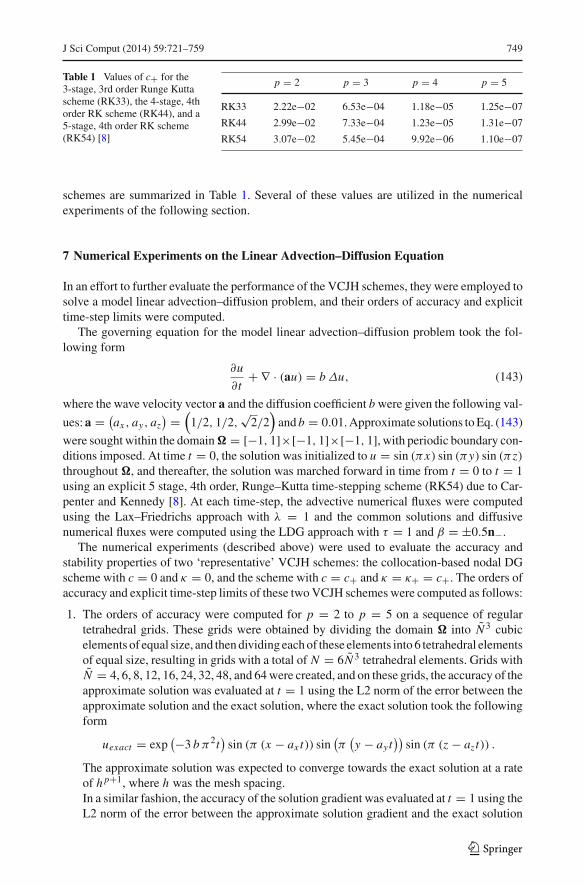
The parameters c and κ have an effect on the explicit time-step limit and the accuracy ofa VCJH scheme. Williams et al. [38] have shown that choosing κ = c and 0 ≤ c ≤ c+yields stable and accurate results for linear advection–diffusion problems on triangles, wherec+ is a value of c that maximizes the explicit time-step limit for linear advection problems.Values of c > c+ were still found to be stable, but resulted in a reduction in the explicittime-step limits and the orders of accuracy of the schemes. In light of these results, it wasdesirable to determine values of c+ for linear advection problems on tetrahedra. In response,Williams [37] employed classical von Neumann analysis (as outlined in [10,21,26,32]) inorder to determine the value of c = c+ that maximizes the explicit time-step limit of the VCJHschemes for a 3D, canonical, linear advection problem. For the sake of completeness, thevalues of c+ (determined in [37]) for different polynomial orders and different time-stepping
123
J Sci Comput (2014) 59:721–759 749
Table 1 Values of c+ for the3-stage, 3rd order Runge Kuttascheme (RK33), the 4-stage, 4thorder RK scheme (RK44), and a5-stage, 4th order RK scheme(RK54) [8]
p = 2 p = 3 p = 4 p = 5
RK33 2.22e−02 6.53e−04 1.18e−05 1.25e−07
RK44 2.99e−02 7.33e−04 1.23e−05 1.31e−07
RK54 3.07e−02 5.45e−04 9.92e−06 1.10e−07
schemes are summarized in Table 1. Several of these values are utilized in the numericalexperiments of the following section.
7 Numerical Experiments on the Linear Advection–Diffusion Equation
In an effort to further evaluate the performance of the VCJH schemes, they were employed tosolve a model linear advection–diffusion problem, and their orders of accuracy and explicittime-step limits were computed.
The governing equation for the model linear advection–diffusion problem took the fol-lowing form
∂u
∂t+ ∇ · (au) = bΔu, (143)
where the wave velocity vector a and the diffusion coefficient b were given the following val-
ues: a = (ax , ay, az
) =(
1/2, 1/2,√
2/2)
and b = 0.01. Approximate solutions to Eq. (143)
were sought within the domain � = [−1, 1]×[−1, 1]×[−1, 1], with periodic boundary con-ditions imposed. At time t = 0, the solution was initialized to u = sin (πx) sin (πy) sin (π z)throughout �, and thereafter, the solution was marched forward in time from t = 0 to t = 1using an explicit 5 stage, 4th order, Runge–Kutta time-stepping scheme (RK54) due to Car-penter and Kennedy [8]. At each time-step, the advective numerical fluxes were computedusing the Lax–Friedrichs approach with λ = 1 and the common solutions and diffusivenumerical fluxes were computed using the LDG approach with τ = 1 and β = ±0.5n−.
The numerical experiments (described above) were used to evaluate the accuracy andstability properties of two ‘representative’ VCJH schemes: the collocation-based nodal DGscheme with c = 0 and κ = 0, and the scheme with c = c+ and κ = κ+ = c+. The orders ofaccuracy and explicit time-step limits of these two VCJH schemes were computed as follows:
1. The orders of accuracy were computed for p = 2 to p = 5 on a sequence of regulartetrahedral grids. These grids were obtained by dividing the domain � into N 3 cubicelements of equal size, and then dividing each of these elements into 6 tetrahedral elementsof equal size, resulting in grids with a total of N = 6N 3 tetrahedral elements. Grids withN = 4, 6, 8, 12, 16, 24, 32, 48, and 64 were created, and on these grids, the accuracy of theapproximate solution was evaluated at t = 1 using the L2 norm of the error between theapproximate solution and the exact solution, where the exact solution took the followingform
uexact = exp(−3 b π2t
)sin (π (x − ax t)) sin
(π(y − ayt
))sin (π (z − azt)) .
The approximate solution was expected to converge towards the exact solution at a rateof h p+1, where h was the mesh spacing.In a similar fashion, the accuracy of the solution gradient was evaluated at t = 1 using theL2 norm of the error between the approximate solution gradient and the exact solution
123
750 J Sci Comput (2014) 59:721–759
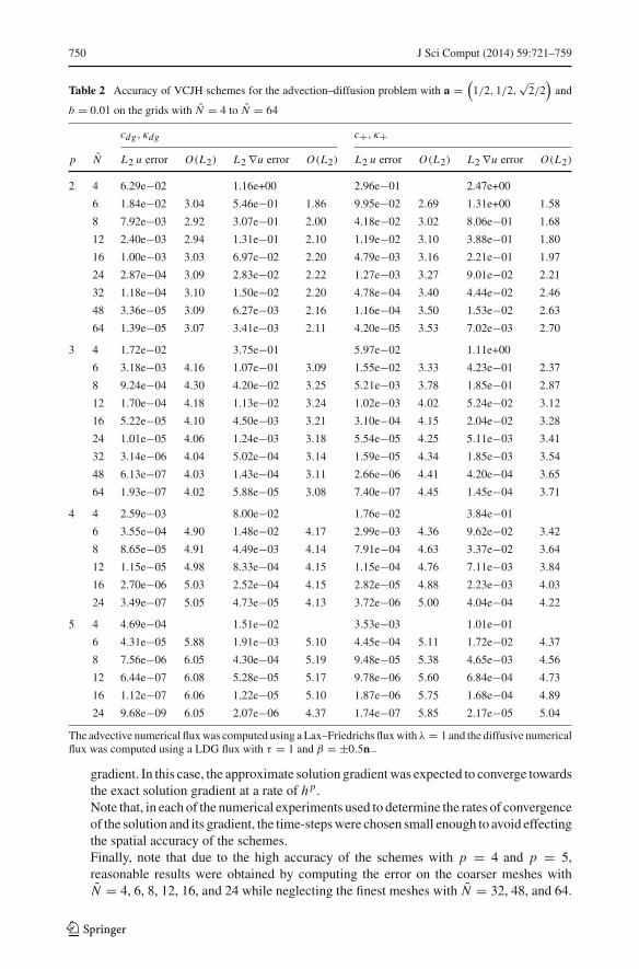
Table 2 Accuracy of VCJH schemes for the advection–diffusion problem with a =(
1/2, 1/2,√
2/2)
and
b = 0.01 on the grids with N = 4 to N = 64
cdg, κdg c+, κ+
p N L2 u error O(L2) L2 ∇u error O(L2) L2 u error O(L2) L2 ∇u error O(L2)
2 4 6.29e−02 1.16e+00 2.96e−01 2.47e+00
6 1.84e−02 3.04 5.46e−01 1.86 9.95e−02 2.69 1.31e+00 1.58
8 7.92e−03 2.92 3.07e−01 2.00 4.18e−02 3.02 8.06e−01 1.68
12 2.40e−03 2.94 1.31e−01 2.10 1.19e−02 3.10 3.88e−01 1.80
16 1.00e−03 3.03 6.97e−02 2.20 4.79e−03 3.16 2.21e−01 1.97
24 2.87e−04 3.09 2.83e−02 2.22 1.27e−03 3.27 9.01e−02 2.21
32 1.18e−04 3.10 1.50e−02 2.20 4.78e−04 3.40 4.44e−02 2.46
48 3.36e−05 3.09 6.27e−03 2.16 1.16e−04 3.50 1.53e−02 2.63
64 1.39e−05 3.07 3.41e−03 2.11 4.20e−05 3.53 7.02e−03 2.70
3 4 1.72e−02 3.75e−01 5.97e−02 1.11e+00
6 3.18e−03 4.16 1.07e−01 3.09 1.55e−02 3.33 4.23e−01 2.37
8 9.24e−04 4.30 4.20e−02 3.25 5.21e−03 3.78 1.85e−01 2.87
12 1.70e−04 4.18 1.13e−02 3.24 1.02e−03 4.02 5.24e−02 3.12
16 5.22e−05 4.10 4.50e−03 3.21 3.10e−04 4.15 2.04e−02 3.28
24 1.01e−05 4.06 1.24e−03 3.18 5.54e−05 4.25 5.11e−03 3.41
32 3.14e−06 4.04 5.02e−04 3.14 1.59e−05 4.34 1.85e−03 3.54
48 6.13e−07 4.03 1.43e−04 3.11 2.66e−06 4.41 4.20e−04 3.65
64 1.93e−07 4.02 5.88e−05 3.08 7.40e−07 4.45 1.45e−04 3.71
4 4 2.59e−03 8.00e−02 1.76e−02 3.84e−01
6 3.55e−04 4.90 1.48e−02 4.17 2.99e−03 4.36 9.62e−02 3.42
8 8.65e−05 4.91 4.49e−03 4.14 7.91e−04 4.63 3.37e−02 3.64
12 1.15e−05 4.98 8.33e−04 4.15 1.15e−04 4.76 7.11e−03 3.84
16 2.70e−06 5.03 2.52e−04 4.15 2.82e−05 4.88 2.23e−03 4.03
24 3.49e−07 5.05 4.73e−05 4.13 3.72e−06 5.00 4.04e−04 4.22
5 4 4.69e−04 1.51e−02 3.53e−03 1.01e−01
6 4.31e−05 5.88 1.91e−03 5.10 4.45e−04 5.11 1.72e−02 4.37
8 7.56e−06 6.05 4.30e−04 5.19 9.48e−05 5.38 4.65e−03 4.56
12 6.44e−07 6.08 5.28e−05 5.17 9.78e−06 5.60 6.84e−04 4.73
16 1.12e−07 6.06 1.22e−05 5.10 1.87e−06 5.75 1.68e−04 4.89
24 9.68e−09 6.05 2.07e−06 4.37 1.74e−07 5.85 2.17e−05 5.04
The advective numerical flux was computed using a Lax–Friedrichs flux withλ = 1 and the diffusive numericalflux was computed using a LDG flux with τ = 1 and β = ±0.5n−
gradient. In this case, the approximate solution gradient was expected to converge towardsthe exact solution gradient at a rate of h p .Note that, in each of the numerical experiments used to determine the rates of convergenceof the solution and its gradient, the time-steps were chosen small enough to avoid effectingthe spatial accuracy of the schemes.Finally, note that due to the high accuracy of the schemes with p = 4 and p = 5,reasonable results were obtained by computing the error on the coarser meshes withN = 4, 6, 8, 12, 16, and 24 while neglecting the finest meshes with N = 32, 48, and 64.
123
J Sci Comput (2014) 59:721–759 751
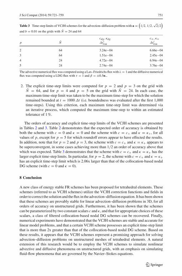
Table 3 Time-step limits of VCJH schemes for the advection–diffusion problem with a =(
1/2, 1/2,√
2/2)
and b = 0.01 on the grids with N = 24 and 64
cdg, κdg c+, κ+p N Δt ′lim Δt ′lim2 64 3.24e−04 6.66e−04
3 64 1.51e−04 2.45e−04
4 24 4.72e−04 6.94e−04
5 24 2.74e−04 3.76e−04
The advective numerical flux was computed using a Lax–Friedrichs flux withλ = 1 and the diffusive numericalflux was computed using a LDG flux with τ = 1 and β = ±0.5n−
2. The explicit time-step limits were computed for p = 2 and p = 3 on the grid withN = 64, and for p = 4 and p = 5 on the grid with N = 24. In each case, themaximum time-step limit was taken to be the maximum time-step for which the solutionremained bounded at t = 1000Δt (i.e. boundedness was evaluated after the first 1,000time-steps). Using this criterion, each maximum time-step limit was determined viaan iterative process, which computed the maximum time-step to within an estimatedtolerance of 1 %.
The orders of accuracy and explicit time-step limits of the VCJH schemes are presentedin Tables 2 and 3. Table 2 demonstrates that the expected order of accuracy is obtained byboth the scheme with c = 0 and κ = 0 and the scheme with c = c+ and κ = κ+, for allvalues of p, except for p = 5 for which roundoff errors appear to have effected the results.In addition, note that for p = 2 and p = 3, the scheme with c = c+ and κ = κ+ appears tobe superconvergent, in some cases achieving more than 1/2 an order of accuracy above thatwhich was expected. Table 3 demonstrates that the scheme with c = c+ and κ = κ+ has thelarger explicit time-step limits. In particular, for p = 2, the scheme with c = c+ and κ = κ+has an explicit time-step limit which is 2.06x larger than that of the collocation-based nodalDG scheme (with c = 0 and κ = 0).
8 Conclusion
A new class of energy stable FR schemes has been proposed for tetrahedral elements. Theseschemes (referred to as VCJH schemes) utilize the VCJH correction functions and fields inorder to correct the solution and the flux in the advection–diffusion equation. It has been shownthat these schemes are provably stable for linear advection–diffusion problems in 3D, for allorders of accuracy on unstructured grids. Furthermore, it has been shown that the schemescan be parameterized by two constant scalars c and κ , and that for appropriate choices of thesescalars, a class of filtered collocation-based nodal DG schemes can be recovered. Finally,numerical experiments have demonstrated that the VCJH schemes are stable and accurate forlinear model problems, and that a certain VCJH scheme possesses an explicit time-step limitthat is more than 2x greater than that of the collocation-based nodal DG scheme. Based onthese results, it appears that the VCJH schemes represent a promising approach for solvingadvection–diffusion problems on unstructured meshes of tetrahedral elements. A naturalextension of this research would be to employ the VCJH schemes to simulate nonlinearadvective and diffusive phenomena on unstructured grids, with an emphasis on simulatingfluid-flow phenomena that are governed by the Navier–Stokes equations.
123
752 J Sci Comput (2014) 59:721–759
Acknowledgments The authors would like to thank the National Science Foundation Graduate ResearchFellowship Program, the Stanford Graduate Fellowships program, the National Science Foundation (Grants0708071 and 0915006), the Air Force Office of Scientific Research (Grants FA9550-07-1-0195 and FA9550-10-1-0418) and NVIDIA for supporting this work.
9 Appendix A: Constructing the Energy Stable (VCJH) Correction Fields
In this section, a procedure will be presented for constructing energy stable (VCJH) correctionfields φ f,l and ψ f,l that satisfy Eqs. (43) and (53), respectively.
9.1 Preliminaries
Recall that φ f,l ≡ ∇ · h f,l and ψ f,l ≡ ∇ · g f,l . In accordance with these definitions, itmay appear natural to first construct precise expressions for the correction functions h f,l andg f,l , and thereafter apply the divergence operator ∇ to these expressions in order to obtainφ f,l and ψ f,l . However, this is not the best approach, as h f,l and g f,l may not be unique. Inparticular, for p > 1 there are an unlimited number of correction functions which have thesame divergence (or effectively, the same correction field). In addition, the implementationof the VCJH approach only requires the precise formulation of the correction fields φ f,l andψ f,l , and not of the correction functions themselves. Specifically, the VCJH approach onlyrequires definitions of the normal components of the correction functions (h f,l · n and g f,l · n)which are given by Eqs. (23) and (24). In what follows, it will be shown that Eqs. (23), (24),(43), and (53) are sufficient for constructing precise definitions of φ f,l and ψ f,l .
9.2 Constructing the Correction Fields φ f,l
One may arrive at a procedure for constructing the correction fields φ f,l by manipulatingEq. (43) and utilizing the definition of h f,l · n (Eqs. (23) and (24)). Recall from section 3,Lemma 3.1, that the correction functions h f,l and correction fields φ f,l are required to satisfyEq. (43), which can be expanded as follows
p+1∑v=1
v∑w=1
cvw D(p,v,w)(∇ · fC
)D(p,v,w)
(� j
)
=∫
�S
(fC · n
)� j d�S −
∫
�S
(∇ · fC
)� j d�S
=p+1∑v=1
v∑w=1
cvw D(p,v,w)
⎛⎝
N f e∑f =1
N f p∑l=1
[(f�f,l − f D
f,l
)· n f,l
]φ f,l
⎞⎠ D(p,v,w)
(� j
)
=∫
�S
⎛⎝
N f e∑f =1
N f p∑l=1
[(f�f,l − f D
f,l
)· n f,l
]h f,l · n
⎞⎠ � j d�S
−∫
�S
⎛⎝
N f e∑f =1
N f p∑l=1
[(f�f,l − f D
f,l
)· n f,l
]φ f,l
⎞⎠ � j d�S . (144)
123
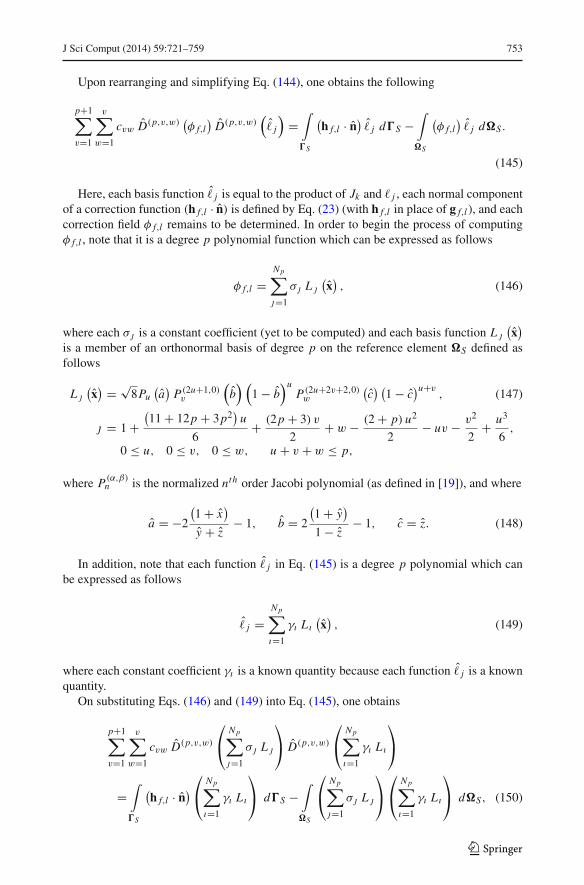
J Sci Comput (2014) 59:721–759 753
Upon rearranging and simplifying Eq. (144), one obtains the following
p+1∑v=1
v∑w=1
cvw D(p,v,w) (φ f,l)
D(p,v,w)(� j
)=∫
�S
(h f,l · n
)� j d�S −
∫
�S
(φ f,l
)� j d�S .
(145)
Here, each basis function � j is equal to the product of Jk and � j , each normal componentof a correction function (h f,l · n) is defined by Eq. (23) (with h f,l in place of g f,l ), and eachcorrection field φ f,l remains to be determined. In order to begin the process of computingφ f,l , note that it is a degree p polynomial function which can be expressed as follows
φ f,l =Np∑j=1
σj Lj(x), (146)
where each σj is a constant coefficient (yet to be computed) and each basis function Lj(x)
is a member of an orthonormal basis of degree p on the reference element �S defined asfollows
Lj(x) = √
8Pu(a)
P(2u+1,0)v
(b) (
1 − b)u
P(2u+2v+2,0)w
(c) (
1 − c)u+v
, (147)
j = 1 +(11 + 12p + 3p2
)u
6+ (2p + 3) v
2+ w − (2 + p) u2
2− uv − v2
2+ u3
6,
0 ≤ u, 0 ≤ v, 0 ≤ w, u + v + w ≤ p,
where P(α,β)n is the normalized nth order Jacobi polynomial (as defined in [19]), and where
a = −2
(1 + x
)
y + z− 1, b = 2
(1 + y
)
1 − z− 1, c = z. (148)
In addition, note that each function � j in Eq. (145) is a degree p polynomial which canbe expressed as follows
� j =Np∑ı=1
γı Lı(x), (149)
where each constant coefficient γı is a known quantity because each function � j is a knownquantity.
On substituting Eqs. (146) and (149) into Eq. (145), one obtains
p+1∑v=1
v∑w=1
cvw D(p,v,w)
⎛⎝
Np∑j=1
σj Lj
⎞⎠ D(p,v,w)
⎛⎝
Np∑ı=1
γı Lı
⎞⎠
=∫
�S
(h f,l · n
)⎛⎝
Np∑ı=1
γı Lı
⎞⎠ d�S −
∫
�S
⎛⎝
Np∑j=1
σj Lj
⎞⎠⎛⎝
Np∑ı=1
γı Lı
⎞⎠ d�S, (150)
123
754 J Sci Comput (2014) 59:721–759
or equivalently
Np∑j=1
σj
p+1∑v=1
v∑w=1
cvw D(p,v,w) (Lj)
D(p,v,w) (Lı )
=∫
�S
(h f,l · n
)Lı d�S −
Np∑j=1
σj
∫
�S
Lj Lı d�S . (151)
Upon noting that Lı and Lj are orthonormal polynomials, one may derive the followingexpression from Eq. (151)
Np∑j=1
σj
p+1∑v=1
v∑w=1
cvw D(p,v,w) (Lj)
D(p,v,w) (Lı ) = −σı +∫
�S
(h f,l · n
)Lı d�S . (152)
Equation (152) holds for ı = 1, . . . , Np and provides a system of Np equations for theNp unknown coefficients σj . Together, Eqs. (152) and (146) completely define φ f,l .
9.3 Constructing the Correction Fields ψ f,l
In following the approach of the previous section, one may arrive at a procedure for con-structing the correction fields ψ f,l by manipulating Eq. (53) and utilizing the definition ofg f,l · n (Eqs. (23) and (24)). Once these manipulations (which are omitted for the sake ofbrevity) are performed, one obtains the following formula for each field ψ f,l
ψ f,l =Np∑j=1
ξj Lj(x), (153)
where the Np unknown coefficients ξj can be obtained from the following system of ı =1, . . . , Np equations
Np∑j=1
ξj
p+1∑v=1
v∑w=1
κvw D(p,v,w) (Lj)
D(p,v,w) (Lı ) = −ξı +∫
�S
(g f,l · n
)Lı d�S . (154)
10 Appendix B: Energy Stable (VCJH) Filter Matrices
This section discusses the procedure for forming the energy stable (VCJH) filter matricesand examines the resulting structure of the filter matrices.
10.1 Procedure for Forming the Filter Matrices
The filters F1 and F2 are obtained from the matrices Mk,Mk,Kk , and Kk via Eq. (142).The mass matrices Mk and Mk can be constructed from inner products of the nodal basisfunctions � j
(x)
in accordance with Eq. (70). However, it is often difficult to compute the nodalbasis functions � j
(x)
directly, and one is often better served by using the orthonormal basisfunctions L j
(x)
in their place. In particular, one may use the orthonormal basis functions todefine a ‘Vandermonde matrix’ Vk which has the following entries
[Vk]i j = L j(xi), (155)
123
J Sci Comput (2014) 59:721–759 755
and next, one may use Vk to compute the mass matrices as follows
Mk = Jk
(Vk
(Vk)T)−1
, (156)
Mk = Jk
⎡⎢⎢⎢⎢⎣
(Vk
(Vk)T)−1
0 0
0(
Vk(Vk)T)−1
0
0 0(
Vk(Vk)T)−1
⎤⎥⎥⎥⎥⎦. (157)
Note that the derivation of Eqs. (156) and (157) is discussed in detail in [19].
In a similar fashion, one may construct expressions for Kk and Kk in terms of the ortho-normal basis functions. Recall that Eqs. (76) and (77) provide expressions for Kk and Kk in
terms of the matrices(
D(p,v,w))T
D(p,v,w), where each D(p,v,w) is a matrix which has the
following entries
[D(p,v,w)]i j = D(p,v,w) (� j(x)) ∣∣∣∣
xi
. (158)
One may use the orthonormal basis functions L j(x)
to construct similar matrices ˆD(p,v,w)which have the following entries
[ ˆD(p,v,w)]i j = D(p,v,w) (L j(x)) ∣∣∣∣
xi
. (159)
One may then relate each ˆD(p,v,w) to each D(p,v,w) by using the following identity
D(p,v,w) = ˆD(p,v,w)(
Vk)−1
. (160)
Note that the derivation of Eq. (160) is discussed in detail in [19].Upon substituting Eq. (160) into Eqs. (76) and (77), one obtains the following expressions
for Kk and Kk
Kk = Jk
Np
p+1∑v=1
v∑w=1
cvw(
Vk)−T
( ˆD(p,v,w))T ˆD(p,v,w)
(Vk)−1
, (161)
Kk = Jk
Np
p+1∑v=1
v∑w=1
κvw
⎡⎢⎢⎢⎢⎢⎢⎢⎣
(Vk)−T
( ˆD(p,v,w))T ˆD(p,v,w) (Vk
)−10 0
0(Vk)−T
( ˆD(p,v,w))T ˆD(p,v,w) (Vk
)−10
0 0(Vk)−T
( ˆD(p,v,w))T ˆD(p,v,w) (Vk
)−1
⎤⎥⎥⎥⎥⎥⎥⎥⎦.
(162)
123
756 J Sci Comput (2014) 59:721–759
Next, on substituting Eqs. (161), (162), (156), and (157) into Eq. (142), one obtains thefollowing expressions for F1 and F2
F1 =⎛⎝I + 1
Np
p+1∑v=1
v∑w=1
cvw Vk( ˆD(p,v,w)
)T ˆD(p,v,w)(
Vk)−1
⎞⎠
−1
= Vk ˆF1
(Vk)−1
, (163)
where
ˆF1 =⎛⎝I + 1
Np
p+1∑v=1
v∑w=1
cvw
( ˆD(p,v,w))T ˆD(p,v,w)
⎞⎠
−1
, (164)
and
F2 =
⎛⎜⎜⎜⎜⎜⎜⎜⎝
I + 1
Np
p+1∑v=1
v∑w=1
κvw
⎡⎢⎢⎢⎢⎢⎢⎢⎣
Vk( ˆD(p,v,w)
)T ˆD(p,v,w) (Vk)−1
0 0
0 Vk( ˆD(p,v,w)
)T ˆD(p,v,w) (Vk)−1
0
0 0 Vk( ˆD(p,v,w)
)T ˆD(p,v,w) (Vk)−1
⎤⎥⎥⎥⎥⎥⎥⎥⎦
⎞⎟⎟⎟⎟⎟⎟⎟⎠
−1
= Vk ˆF2
(Vk)−1
, (165)
where
ˆF2 =
⎛⎜⎜⎜⎜⎜⎜⎜⎝
I + 1
Np
p+1∑v=1
v∑w=1
κvw
⎡⎢⎢⎢⎢⎢⎢⎢⎣
( ˆD(p,v,w))T ˆD(p,v,w) 0 0
0( ˆD(p,v,w)
)T ˆD(p,v,w) 0
0 0( ˆD(p,v,w)
)T ˆD(p,v,w)
⎤⎥⎥⎥⎥⎥⎥⎥⎦
⎞⎟⎟⎟⎟⎟⎟⎟⎠
−1
,
(166)
and
Vk =⎡⎣
Vk 0 00 Vk 00 0 Vk
⎤⎦ . (167)
Note that Eqs. (164) and (166) define new filtering matrices ˆF1 and ˆF2. These matricescan be viewed as filters which act on the orthonormal basis (in contrast to F1 and F2 whichcan be viewed as filters which act on the nodal basis). Conveniently, the two sets of filtersare related via left and right multiplication by the Vandermonde matrix and its inverse (asshown in Eqs. (163) and (165)).
Now, having established a method for constructing F1 and F2 using the orthornormal basis
(via ˆF1 and ˆF2), one may obtain insights into the overall effects of the filtering process by
examining the sparsity patterns of ˆF1 and ˆF2.
123
J Sci Comput (2014) 59:721–759 757
10.2 Sparsity Patterns of the Filter Matrices
On evaluating Eq. (164), one finds that ˆF1 has the following block structure
ˆF1 =[
IB1 00 FB
1
], (168)
where IB1 ∈ R
N �p×N �
p is an identity matrix, FB1 ∈ R
N up×N u
p is a dense matrix of filteringcoefficients, N �
p = Np − N up is the number of orthonormal basis functions of degree ≤
(p − 1), and N up = 1
2 (p + 1) (p + 2) is the number of orthonormal basis functions of
degree p. The structure of ˆF1 ensures that only the degree p orthonormal basis functions areeffected by the filtering matrix. All basis functions of degree ≤ (p − 1) are multiplied bythe identity matrix and remain unaffected.
Similarly, on evaluating Eq. (166), one finds that ˆF2 has the following structure
ˆF2 =
⎡⎢⎢⎢⎢⎢⎢⎢⎢⎢⎢⎢⎣
IB2 0 · · · · · · · · · 0
0 FB2. . .
....... . . IB
2 0...
... 0 FB2. . .
......
. . . IB2 0
0 · · · · · · · · · 0 FB2
⎤⎥⎥⎥⎥⎥⎥⎥⎥⎥⎥⎥⎦
, (169)
where IB2 ∈ R
N �p×N �
p is an identity matrix and FB2 ∈ R
N up×N u
p is a dense matrix of filtering
coefficients. The structure of ˆF2 is similar to the structure of ˆF1, as the structure of ˆF2 alsoensures that only the degree p orthonormal basis functions are effected by the filtering matrix.
In summary, the filters F1 and F2 are related (via the Vandermonde matrix) to the filtersˆF1 and ˆF2 which act on the orthonormal basis functions L j (x), and effect only the highest
(degree p) modes of the residual and the auxiliary variable, respectively.
References
1. Allaneau, Y., Jameson, A.: Connections between the filtered discontinuous Galerkin method and theflux reconstruction approach to high order discretizations. Comput. Methods Appl. Mech. Eng. 200(49),3628–3636 (2011)
2. Arnold, D.N.: An interior penalty finite element method with discontinuous elements. SIAM J. Numer.Anal. 19(4), 742–760 (1982)
3. Bassi, F., Rebay, S.: Accurate 2D Euler computations by means of a high order discontinuous finiteelement method. In: 14th International Conference on Numerical Methods in Fluid Dynamics. Bangalor,India (1994)
4. Bassi, F., Rebay, S.: Discontinuous finite element high order accurate numerical solution of the compress-ible Navier–Stokes equations. In: ICFD Conference on Numerical Methods in Fluid Dynamics. Universityof Oxford, Oxford, England (1995)
5. Bassi, F., Rebay, S.: A high-order accurate discontinuous finite element method for the numerical solutionof the compressible Navier–Stokes equations. J. Comput. Phys. 131(2), 267–279 (1997)
6. Bassi, F., Rebay, S., Mariotti, G., Pedinotti, S., Savini, M.: A high-order accurate discontinuous finiteelement method for inviscid and viscous turbomachinery flows. In: Decuypere, R., Dibelius, G. (eds.) 2ndEuropean Conference on Turbomachinery Fluid Dynamics and Thermodynamics. Antwerpen, Belgium(1997)
123
758 J Sci Comput (2014) 59:721–759
7. Brady, M., Horn, B.K.P.: Rotationally symmetric operators for surface interpolation. Comput. Vis. Graph.Image Process. 22(1), 70–94 (1983)
8. Carpenter, M.H., Kennedy, C.: Fourth-Order 2N-Storage Runge–Kutta Schemes. Tech. Rep. TM 109112,NASA, Langley Research Center (1994)
9. Castonguay, P.: High-Order Energy Stable Flux Reconstruction Schemes for Fluid Flow Simulations onUnstructured Grids. Ph.D. Thesis, Stanford University (2012)
10. Castonguay, P., Vincent, P.E., Jameson, A.: A new class of high-order energy stable flux reconstructionschemes for conservation laws on triangular grids. J. Sci. Comput. 51(1), 224–256 (2011)
11. Cockburn, B., Hou, S., Shu, C.W.: The Runge–Kutta local projection discontinuous Galerkin finite elementmethod for conservation laws IV: the multidimensional case. Math. Comput. 54(190), 545–581 (1990)
12. Cockburn, B., Shu, C.W.: The local discontinuous Galerkin method for time-dependent convection-diffusion systems. SIAM J. Numer. Anal. 35(6), 2440–2463 (1998)
13. Danielsson, P.E., Seger, O.: Rotation invariance in gradient and higher order derivative detectors. Comput.Vis. Graph. Image Process. 49(2), 198–221 (1990)
14. Friedrichs, K.O.: Symmetric hyperbolic linear differential equations. Commun. Pure Appl. Math. 7, 345–392 (1954)
15. Gao, H., Wang, Z.J.: A high-order lifting collocation penalty formulation for the Navier–Stokes equationson 2D mixed grids. In: 19th AIAA Computational Fluid Dynamics. San Antonio, TX (2009)
16. Grimson, W.E.L.: From Images to Surfaces: A Computational Study of the Human Early Visual System.MIT Press, Cambridge (1981)
17. Haga, T., Gao, H., Wang, Z.J.: A high-order unifying discontinuous formulation for 3D mixed grids. In:48th AIAA Aerospace Sciences Meeting. Orlando, FL (2010)
18. Haga, T., Gao, H., Wang, Z.J.: A high-order unifying discontinuous formulation for the Navier–Stokesequations on 3D mixed grids. Mathe. Model. Nat. Phenom. 6(3), 28–56 (2011)
19. Hesthaven, J.S., Warburton, T.: Nodal Discontinuous Galerkin Methods: Algorithms, Analysis, and Appli-cations. Springer, Berlin (2007)
20. Hirsch, C.: Numerical Computation of Internal and External Flows: The Fundamentals of ComputationalFluid Dynamics, Volume I. Butterworth-Heinemann, London (2007)
21. Hu, F.Q., Hussaini, M.Y., Rasetarinera, P.: An analysis of the discontinuous Galerkin method for wavepropagation problems. J. Comput. Phys. 151(2), 921–946 (1999)
22. Huynh, H.T.: A flux reconstruction approach to high-order schemes including discontinuous Galerkinmethods. In: 18th AIAA Computational Fluid Dynamics Conference. Miami, FL (2007)
23. Huynh, H.T.: A reconstruction approach to high-order schemes including discontinuous Galerkin fordiffusion. In: 47th AIAA Aerospace Sciences Meeting. Orlando, FL (2009)
24. Huynh, H.T.: High-order methods including discontinuous Galerkin by reconstructions on triangularmeshes. In: 49th AIAA Aerospace Sciences Meeting. Orlando, FL (2011)
25. Jameson, A.: A proof of the stability of the spectral difference method for all orders of accuracy. J. Sci.Comput. 45(1), 348–358 (2010)
26. Kannan, R., Wang, Z.J.: LDG2: a variant of the LDG flux formulation for the spectral volume method. J.Sci. Comput. 46(2), 314–328 (2011)
27. Kopriva, D.A., Kolias, J.H.: A conservative staggered-grid Chebyshev multidomain method for com-pressible flows. J. Comput. Phys. 125, 244–261 (1996)
28. Lax, P.D.: Weak solutions of nonlinear hyperbolic equations and their numerical computation. Commun.Pure Appl. Math. 7, 159–193 (1954)
29. Liu, Y., Vinokur, M., Wang, Z.J.: Spectral difference method for unstructured grids I: basic formulation.J. Comput. Phys. 216, 780–801 (2006)
30. Peraire, J., Persson, P.O.: The compact discontinuous Galerkin (CDG) method for elliptic problems.SIAM J. Sci. Comput. 30(4), 1806–1824 (2009)
31. Raviart, P., Thomas, J.: A mixed finite element method for second-order elliptic problems. In: Mathemat-ical Aspects of Finite Element Methods, pp. 292–315. Springer, Berlin (1977)
32. Van den Abeele, K., Lacor, C.: An accuracy and stability study of the 2D spectral volume method. J.Comput. Phys. 226(1), 1007–1026 (2007)
33. Vincent, P.E., Castonguay, P., Jameson, A.: A new class of high-order energy stable flux reconstructionschemes. J. Sci. Comput. 47(1), 50–72 (2011)
34. Vincent, P.E., Jameson, A.: Facilitating the adoption of unstructured high-order methods amongst a widercommunity of fluid dynamicists. Math. Model. Nat. Phenom. 6(3), 97–140 (2011)
35. Wang, Z.J., Gao, H.: A unifying lifting collocation penalty formulation for the Euler equations on mixedgrids. In: AIAA P. 47th AIAA Aerospace Sciences Meeting, Orlando, FL, Jan. 5–8 (2009)
123

J Sci Comput (2014) 59:721–759 759
36. Wang, Z.J., Gao, H.: A unifying lifting collocation penalty formulation including the discontinuousGalerkin, spectral volume/difference methods for conservation laws on mixed grids. J. Comput. Phys.228(21), 8161–8186 (2009)
37. Williams, D.M.: Energy Stable High-Order Methods for Simulating Unsteady, Viscous, CompressibleFlows on Unstructured Grids. Ph.D. Thesis, Stanford University (2013)
38. Williams, D.M., Castonguay, P., Vincent, P.E., Jameson, A.: Energy stable flux reconstruction schemesfor advection–diffusion problems on triangles. J. Comput. Phys. 250, 53–76 (2013)
39. Yu, M., Wang, Z.J.: On the connection between the correction and weighting functions in the correctionprocedure via reconstruction method. J. Sci. Comput. 54(1), 227–244 (2012)
123


![spectral and vector analysis on fractafoldshelper.ipam.ucla.edu/publications/iagws3/iagws3_11241.pdfSpectral analysis on nitely rami ed symmetric fractafolds [Strichartz et al] I 2](https://img.pdfslide.us/doc/110x75/5fac21835c40f93c5008cb56/spectral-and-vector-analysis-on-spectral-analysis-on-nitely-rami-ed-symmetric-fractafolds.jpg)