Embed Size (px)
Citation preview
Energy & Society Energy Units and Fundamentals
1
Toolkit 1:
Energy Units and Fundamentals of
Quantitative Analysis
Energy & Society Energy Units and Fundamentals
2
Table of Contents
1. Key Concepts: Force, Work, Energy & Power 3 2. Orders of Magnitude & Scientific Notation 6
2.1. Orders of Magnitude 6 2.2. Scientific Notation 7 2.3. Rules for Calculations 7
2.3.1. Multiplication 8 2.3.2. Division 8 2.3.3. Exponentiation 8 2.3.4. Square Root 8 2.3.5. Addition & Subtraction 9
3. Linear versus Exponential Growth 10 3.1. Linear Growth 10 3.2. Exponential Growth 11
4. Uncertainty & Significant Figures 14 4.1. Uncertainty 14 4.2. Significant Figures 15 4.3. Exact Numbers 15 4.4. Identifying Significant Figures 16 4.5. Rules for Calculations 17
4.5.1. Addition & Subtraction 17 4.5.2. Multiplication, Division & Exponentiation 18
5. Unit Analysis 19 5.1. Commonly Used Energy & Non-energy Units 20 5.2. Form & Function 21
6. Sample Problems 22 6.1. Scientific Notation 22 6.2. Linear & Exponential Growth 22 6.3. Significant Figures 23 6.4. Unit Conversions 23
7. Answers to Sample Problems 24 7.1. Scientific Notation 24 7.2. Linear & Exponential Growth 24 7.3. Significant Figures 24 7.4. Unit Conversions 26
8. References 27
Energy & Society Energy Units and Fundamentals
3
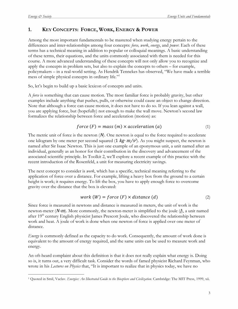
1. KEY CONCEPTS: FORCE, WORK, ENERGY & POWER
Among the most important fundamentals to be mastered when studying energy pertain to the differences and inter-relationships among four concepts: force, work, energy, and power. Each of these terms has a technical meaning in addition to popular or colloquial meanings. A basic understanding of these terms, their equations, and the units commonly associated with them is needed for this course. A more advanced understanding of these concepts will not only allow you to recognize and apply the concepts in problem sets, but also to explain the concepts to others – for example, policymakers – in a real-world setting. As Hendrik Tennekes has observed, “We have made a terrible mess of simple physical concepts in ordinary life.”1
So, let’s begin to build up a basic lexicon of concepts and units.
A force is something that can cause motion. The most familiar force is probably gravity, but other examples include anything that pushes, pulls, or otherwise could cause an object to change direction. Note that although a force can cause motion, it does not have to do so. If you lean against a wall, you are applying force, but (hopefully) not enough to make the wall move. Newton’s second law formalizes the relationship between force and acceleration (motion) as:
𝑓𝑜𝑟𝑐𝑒 𝐹 = 𝑚𝑎𝑠𝑠 𝑚 × 𝑎𝑐𝑐𝑒𝑙𝑒𝑟𝑎𝑡𝑖𝑜𝑛 (𝑎) (1)
The metric unit of force is the newton (N). One newton is equal to the force required to accelerate one kilogram by one meter per second squared (1 kg· m⁄s2). As you might suspect, the newton is named after Sir Isaac Newton. This is just one example of an eponymous unit, a unit named after an individual, generally as an honor for their contribution in the discovery and advancement of the associated scientific principle. In Toolkit 2, we’ll explore a recent example of this practice with the recent introduction of the Rosenfeld, a unit for measuring electricity savings.
The next concept to consider is work, which has a specific, technical meaning referring to the application of force over a distance. For example, lifting a heavy box from the ground to a certain height is work; it requires energy. To lift the box, you have to apply enough force to overcome gravity over the distance that the box is elevated:
𝑤𝑜𝑟𝑘 𝑊 = 𝑓𝑜𝑟𝑐𝑒 𝐹 × 𝑑𝑖𝑠𝑡𝑎𝑛𝑐𝑒 (𝑑) (2)
Since force is measured in newtons and distance is measured in meters, the unit of work is the newton-meter (N‐m). More commonly, the newton-meter is simplified to the joule (J), a unit named after 19th century English physicist James Prescott Joule, who discovered the relationship between work and heat. A joule of work is done when one newton of force is applied over one meter of distance.
Energy is commonly defined as the capacity to do work. Consequently, the amount of work done is equivalent to the amount of energy required, and the same units can be used to measure work and energy.
An oft-heard complaint about this definition is that it does not really explain what energy is. Doing so is, it turns out, a very difficult task. Consider the words of famed physicist Richard Feynman, who wrote in his Lectures on Physics that, “It is important to realize that in physics today, we have no
1 Quoted in Smil, Vaclav. Energies: An Illustrated Guide to the Biosphere and Civilization. Cambridge: The MIT Press, 1999, xii.
Energy & Society Energy Units and Fundamentals
4
knowledge of what energy is. We do not have a picture that energy comes in little blobs of a definite amount.” Alternately, David Rose, one of the founding members of MIT’s nuclear engineering program, famously described energy as “an abstract concept invented by physical scientists in the nineteenth century to describe quantitatively a wide variety of natural phenomena.”
The common definition of energy provides a sort of working definition that should help you with your calculations. A deeper understanding of energy can be achieved by exploring some of the fundamental principles of physics. These principles will be previewed here and elaborated upon further in later Toolkits, as needed.
The first principle is the equivalence of mass and energy, a concept tidily summed up by the well-known (although perhaps not equally well understood) equation 𝐸 = 𝑚𝑐!, where E is energy, m is mass, and c is the speed of light.
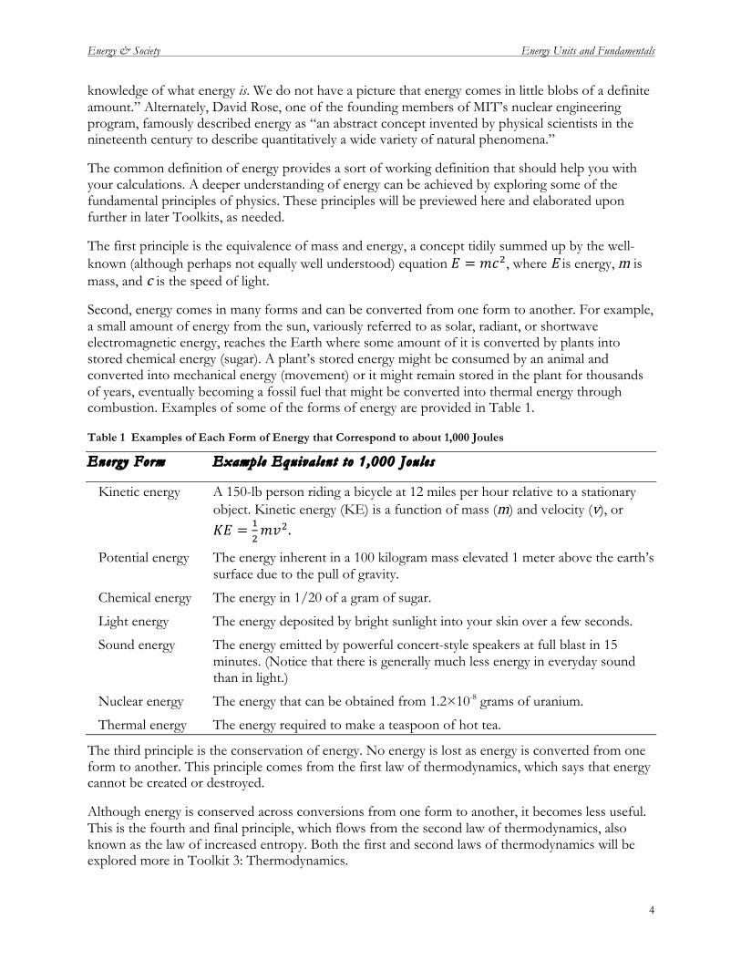
Second, energy comes in many forms and can be converted from one form to another. For example, a small amount of energy from the sun, variously referred to as solar, radiant, or shortwave electromagnetic energy, reaches the Earth where some amount of it is converted by plants into stored chemical energy (sugar). A plant’s stored energy might be consumed by an animal and converted into mechanical energy (movement) or it might remain stored in the plant for thousands of years, eventually becoming a fossil fuel that might be converted into thermal energy through combustion. Examples of some of the forms of energy are provided in Table 1.
Table 1 Examples of Each Form of Energy that Correspond to about 1,000 Joules
Energy Form Example Equivalent to 1,000 Joules
Kinetic energy A 150-lb person riding a bicycle at 12 miles per hour relative to a stationary object. Kinetic energy (KE) is a function of mass (m) and velocity (v), or 𝐾𝐸 = !
!𝑚𝑣!.
Potential energy The energy inherent in a 100 kilogram mass elevated 1 meter above the earth’s surface due to the pull of gravity.
Chemical energy The energy in 1/20 of a gram of sugar.
Light energy The energy deposited by bright sunlight into your skin over a few seconds.
Sound energy The energy emitted by powerful concert-style speakers at full blast in 15 minutes. (Notice that there is generally much less energy in everyday sound than in light.)
Nuclear energy The energy that can be obtained from 1.2×10⁻⁸ grams of uranium.
Thermal energy The energy required to make a teaspoon of hot tea.
The third principle is the conservation of energy. No energy is lost as energy is converted from one form to another. This principle comes from the first law of thermodynamics, which says that energy cannot be created or destroyed.
Although energy is conserved across conversions from one form to another, it becomes less useful. This is the fourth and final principle, which flows from the second law of thermodynamics, also known as the law of increased entropy. Both the first and second laws of thermodynamics will be explored more in Toolkit 3: Thermodynamics.
Energy & Society Energy Units and Fundamentals
5
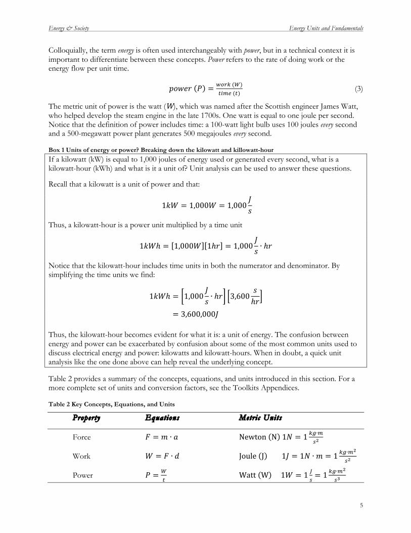
Colloquially, the term energy is often used interchangeably with power, but in a technical context it is important to differentiate between these concepts. Power refers to the rate of doing work or the energy flow per unit time.
𝑝𝑜𝑤𝑒𝑟 𝑃 = !"#$ (!)!"#! (!)
(3)
The metric unit of power is the watt (W), which was named after the Scottish engineer James Watt, who helped develop the steam engine in the late 1700s. One watt is equal to one joule per second. Notice that the definition of power includes time: a 100-watt light bulb uses 100 joules every second and a 500-megawatt power plant generates 500 megajoules every second.
Box 1 Units of energy or power? Breaking down the kilowatt and killowatt-hour
If a kilowatt (kW) is equal to 1,000 joules of energy used or generated every second, what is a kilowatt-hour (kWh) and what is it a unit of? Unit analysis can be used to answer these questions.
Recall that a kilowatt is a unit of power and that:
1𝑘𝑊 = 1,000𝑊 = 1,000𝐽𝑠
Thus, a kilowatt-hour is a power unit multiplied by a time unit
1𝑘𝑊ℎ = 1,000𝑊 1ℎ𝑟 = 1,000𝐽𝑠 ∙ ℎ𝑟
Notice that the kilowatt-hour includes time units in both the numerator and denominator. By simplifying the time units we find:
1𝑘𝑊ℎ = 1,000𝐽𝑠 ∙ ℎ𝑟 3,600
𝑠ℎ𝑟
= 3,600,000𝐽
Thus, the kilowatt-hour becomes evident for what it is: a unit of energy. The confusion between energy and power can be exacerbated by confusion about some of the most common units used to discuss electrical energy and power: kilowatts and kilowatt-hours. When in doubt, a quick unit analysis like the one done above can help reveal the underlying concept.
Table 2 provides a summary of the concepts, equations, and units introduced in this section. For a more complete set of units and conversion factors, see the Toolkits Appendices.
Table 2 Key Concepts, Equations, and Units
Property Equations Metr i c Units
Force 𝐹 = 𝑚 ∙ 𝑎 Newton N 1𝑁 = 1 !"∙!!!
Work 𝑊 = 𝐹 ∙ 𝑑 Joule J 1𝐽 = 1𝑁 ∙𝑚 = 1 !"∙!!
!!
Power 𝑃 = !!
Watt W 1𝑊 = 1 !!= 1 !"∙!
!
!!
Energy & Society Energy Units and Fundamentals
6
2. ORDERS OF MAGNITUDE & SCIENTIFIC NOTATION
2.1. Orders of Magnitude
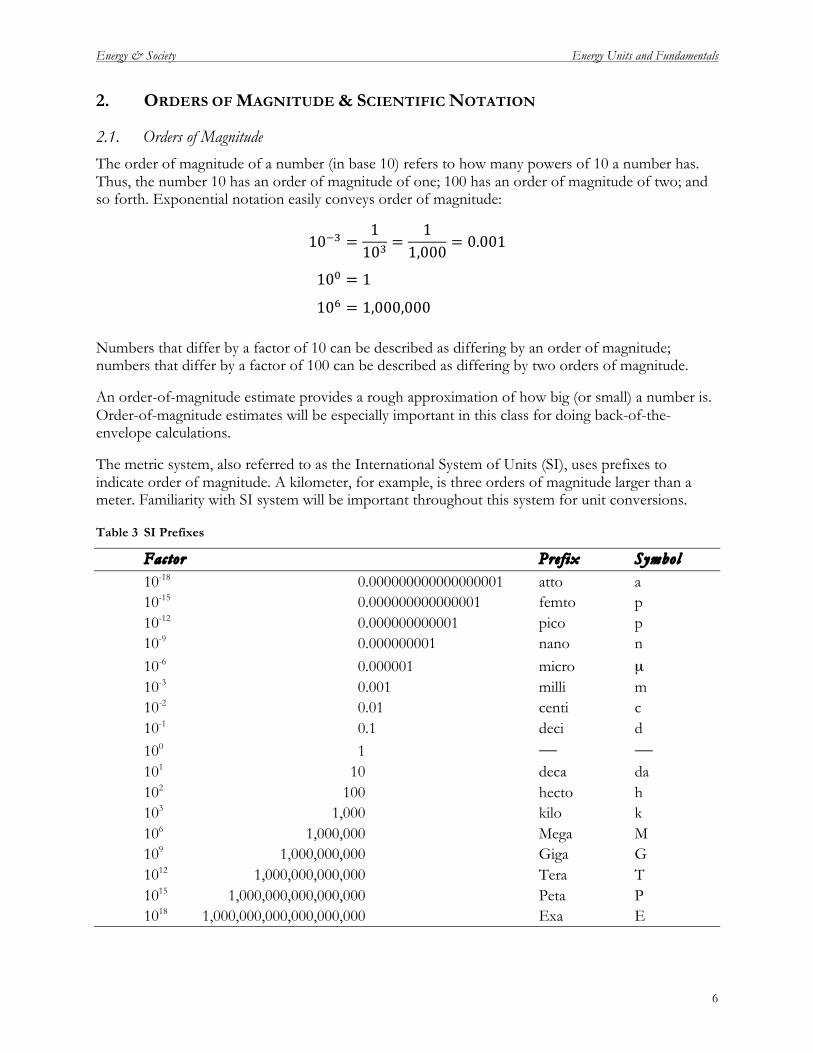
The order of magnitude of a number (in base 10) refers to how many powers of 10 a number has. Thus, the number 10 has an order of magnitude of one; 100 has an order of magnitude of two; and so forth. Exponential notation easily conveys order of magnitude:
10!! =110! =
11,000 = 0.001
10! = 1
10! = 1,000,000
Numbers that differ by a factor of 10 can be described as differing by an order of magnitude; numbers that differ by a factor of 100 can be described as differing by two orders of magnitude.
An order-of-magnitude estimate provides a rough approximation of how big (or small) a number is. Order-of-magnitude estimates will be especially important in this class for doing back-of-the-envelope calculations.
The metric system, also referred to as the International System of Units (SI), uses prefixes to indicate order of magnitude. A kilometer, for example, is three orders of magnitude larger than a meter. Familiarity with SI system will be important throughout this system for unit conversions.
Table 3 SI Prefixes
Factor Pre f ix Symbol 10-18 0.000000000000000001 atto a 10-15 0.000000000000001 femto p 10-12 0.000000000001 pico p 10-9 0.000000001 nano n 10-6 0.000001 micro µ 10-3 0.001 milli m 10-2 0.01 centi c 10-1 0.1 deci d 100 1 101 10 deca da 102 100 hecto h 103 1,000 kilo k 106 1,000,000 Mega M 109 1,000,000,000 Giga G 1012 1,000,000,000,000 Tera T 1015 1,000,000,000,000,000 Peta P 1018 1,000,000,000,000,000,000 Exa E
Energy & Society Energy Units and Fundamentals
7
2.2. Scientific Notation
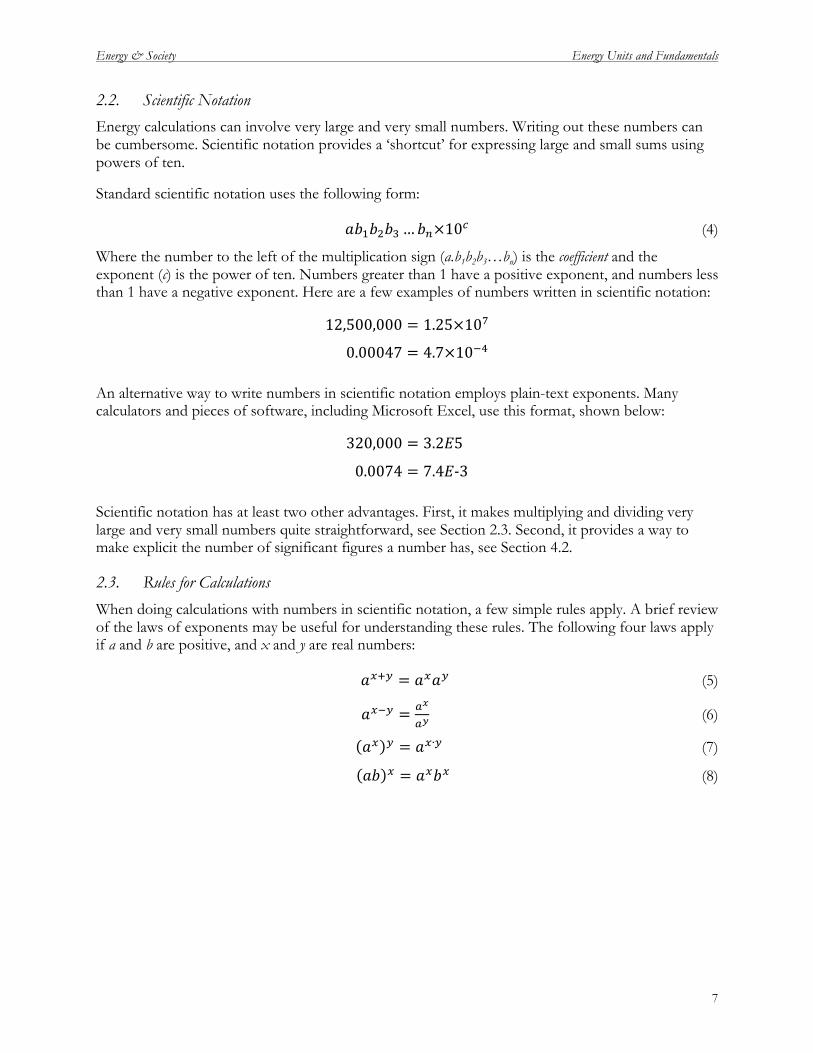
Energy calculations can involve very large and very small numbers. Writing out these numbers can be cumbersome. Scientific notation provides a ‘shortcut’ for expressing large and small sums using powers of ten.
Standard scientific notation uses the following form:
𝑎𝑏!𝑏!𝑏!… 𝑏!×10! (4)
Where the number to the left of the multiplication sign (a.b1b2b3…bn) is the coefficient and the exponent (c) is the power of ten. Numbers greater than 1 have a positive exponent, and numbers less than 1 have a negative exponent. Here are a few examples of numbers written in scientific notation:
12,500,000 = 1.25×10!
0.00047 = 4.7×10!!
An alternative way to write numbers in scientific notation employs plain-text exponents. Many calculators and pieces of software, including Microsoft Excel, use this format, shown below:
320,000 = 3.2𝐸5
0.0074 = 7.4𝐸‐3
Scientific notation has at least two other advantages. First, it makes multiplying and dividing very large and very small numbers quite straightforward, see Section 2.3. Second, it provides a way to make explicit the number of significant figures a number has, see Section 4.2.
2.3. Rules for Calculations
When doing calculations with numbers in scientific notation, a few simple rules apply. A brief review of the laws of exponents may be useful for understanding these rules. The following four laws apply if a and b are positive, and x and y are real numbers:
𝑎!!! = 𝑎!𝑎! (5)
𝑎!!! = !!
!! (6)
𝑎! ! = 𝑎!∙! (7)
𝑎𝑏 ! = 𝑎!𝑏! (8)
Energy & Society Energy Units and Fundamentals
8
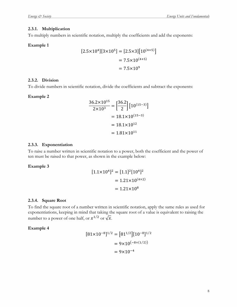
2.3.1. Multiplication To multiply numbers in scientific notation, multiply the coefficients and add the exponents:
Example 1 2.5×10! 3×10! = 2.5×3 10 !!!
= 7.5×10 !!!
= 7.5×10!
2.3.2. Division To divide numbers in scientific notation, divide the coefficients and subtract the exponents:
Example 2 36.2×10!"
2×10! =36.22 10 !"!!
= 18.1×10 !"!!
= 18.1×10!"
= 1.81×10!!
2.3.3. Exponentiation To raise a number written in scientific notation to a power, both the coefficient and the power of ten must be raised to that power, as shown in the example below:
Example 3 1.1×10! ! = 1.1 ! 10! !
= 1.21×10 !×!
= 1.21×10!
2.3.4. Square Root To find the square root of a number written in scientific notation, apply the same rules as used for exponentiations, keeping in mind that taking the square root of a value is equivalent to raising the number to a power of one half, or 𝑥! ! or 𝑥.
Example 4 81×10!! ! ! = 81!/! 10!! ! !
= 9×10 !!× ! !
= 9×10!!
Energy & Society Energy Units and Fundamentals
9
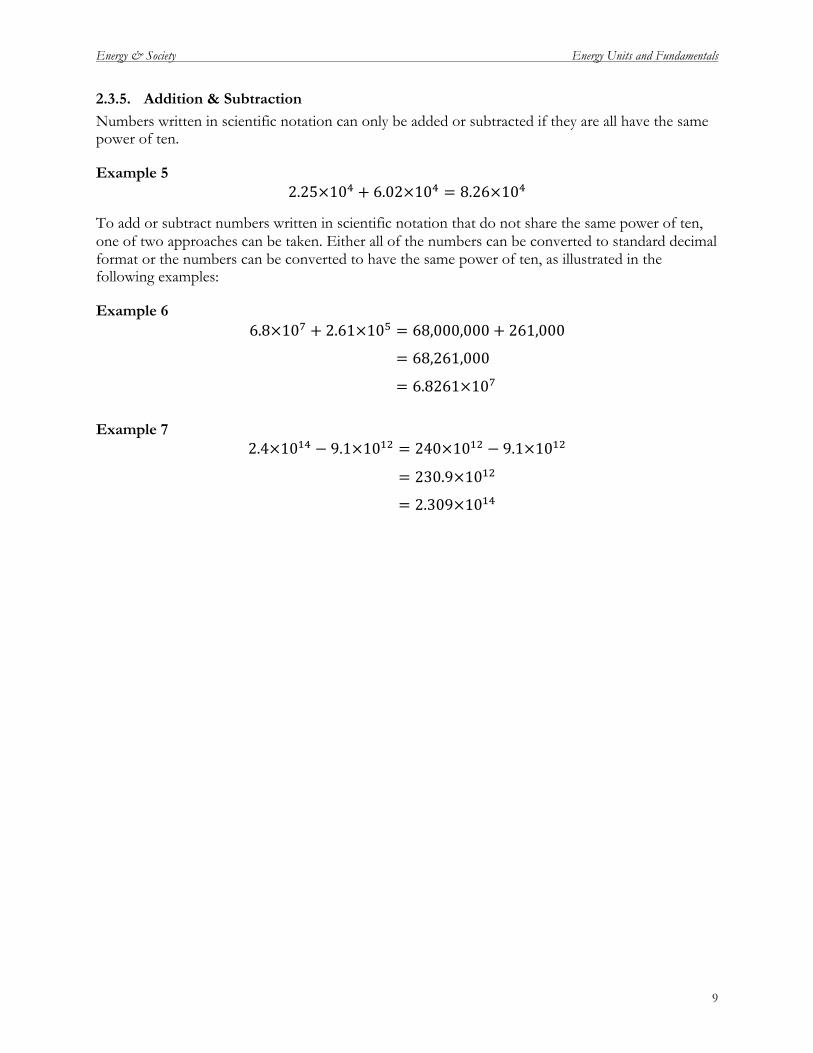
2.3.5. Addition & Subtraction Numbers written in scientific notation can only be added or subtracted if they are all have the same power of ten.
Example 5 2.25×10! + 6.02×10! = 8.26×10!
To add or subtract numbers written in scientific notation that do not share the same power of ten, one of two approaches can be taken. Either all of the numbers can be converted to standard decimal format or the numbers can be converted to have the same power of ten, as illustrated in the following examples:
Example 6 6.8×10! + 2.61×10! = 68,000,000+ 261,000
= 68,261,000
= 6.8261×10!
Example 7 2.4×10!" − 9.1×10!" = 240×10!" − 9.1×10!"
= 230.9×10!"
= 2.309×10!"
Energy & Society Energy Units and Fundamentals
10
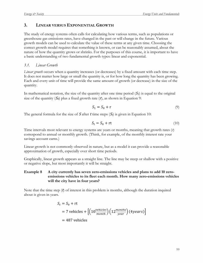
3. LINEAR VERSUS EXPONENTIAL GROWTH
The study of energy systems often calls for calculating how various terms, such as populations or greenhouse gas emissions rates, have changed in the past or will change in the future. Various growth models can be used to calculate the value of these terms at any given time. Choosing the correct growth model requires that something is known, or can be reasonably assumed, about the nature of how the quantity grows or shrinks. For the purposes of this course, it is important to have a basic understanding of two fundamental growth types: linear and exponential.
3.1. Linear Growth
Linear growth occurs when a quantity increases (or decreases) by a fixed amount with each time step. It does not matter how large or small the quantity is, or for how long the quantity has been growing. Each and every unit of time will provide the same amount of growth (or decrease) in the size of the quantity.
In mathematical notation, the size of the quantity after one time period (S1) is equal to the original size of the quantity (S0) plus a fixed growth rate (r), as shown in Equation 9:
𝑆! = 𝑆! + r (9)
The general formula for the size of S after t time steps (St) is given in Equation 10:
𝑆! = 𝑆! + rt (10)
Time intervals most relevant to energy systems are years or months, meaning that growth rates (r) correspond to annual or monthly growth. (Think, for example, of the monthly interest rate your savings account earns.)
Linear growth is not commonly observed in nature, but as a model it can provide a reasonable approximation of growth, especially over short time periods.
Graphically, linear growth appears as a straight line. The line may be steep or shallow with a positive or negative slope, but most importantly it will be straight.
Example 8 A city currently has seven zero-emissions vehicles and plans to add 10 zero-emissions vehicles to its fleet each month. How many zero-emissions vehicles will the city have in four years?
Note that the time step (t) of interest in this problem is months, although the duration inquired about is given in years.
𝑆! = 𝑆! + rt
= 7 vehicles+ 10!"!!"#$%!"#$!
12!"#$!!!"#$
4𝑦𝑒𝑎𝑟𝑠
= 487 vehicles
Energy & Society Energy Units and Fundamentals
11
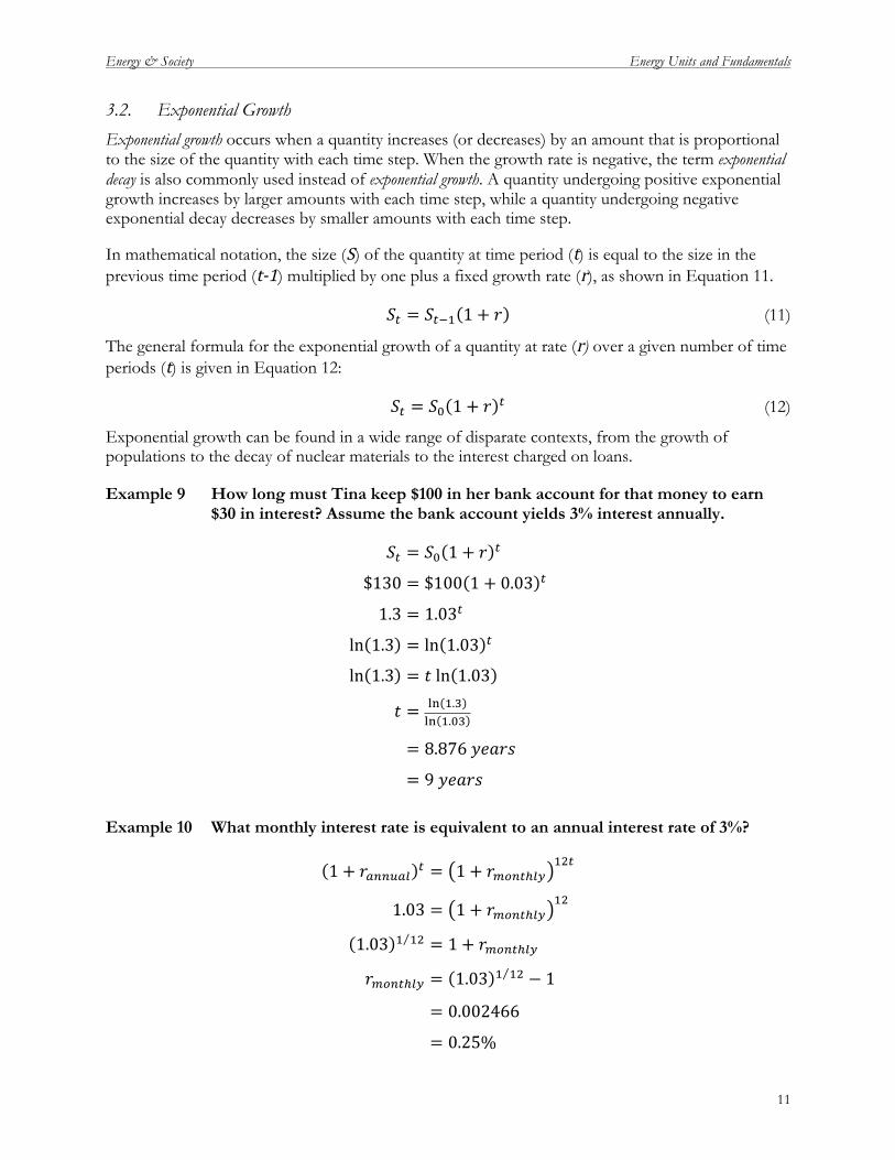
3.2. Exponential Growth
Exponential growth occurs when a quantity increases (or decreases) by an amount that is proportional to the size of the quantity with each time step. When the growth rate is negative, the term exponential decay is also commonly used instead of exponential growth. A quantity undergoing positive exponential growth increases by larger amounts with each time step, while a quantity undergoing negative exponential decay decreases by smaller amounts with each time step.
In mathematical notation, the size (S) of the quantity at time period (t) is equal to the size in the previous time period (t‐1) multiplied by one plus a fixed growth rate (r), as shown in Equation 11.
𝑆! = 𝑆!!! 1+ 𝑟 (11)
The general formula for the exponential growth of a quantity at rate (r) over a given number of time periods (t) is given in Equation 12:
𝑆! = 𝑆! 1+ 𝑟 ! (12)
Exponential growth can be found in a wide range of disparate contexts, from the growth of populations to the decay of nuclear materials to the interest charged on loans.
Example 9 How long must Tina keep $100 in her bank account for that money to earn $30 in interest? Assume the bank account yields 3% interest annually.
𝑆! = 𝑆! 1+ 𝑟 !
$130 = $100 1+ 0.03 !
1.3 = 1.03!
ln 1.3 = ln 1.03 !
ln 1.3 = 𝑡 ln 1.03
𝑡 = !" !.!!" !.!"
= 8.876 𝑦𝑒𝑎𝑟𝑠
= 9 𝑦𝑒𝑎𝑟𝑠
Example 10 What monthly interest rate is equivalent to an annual interest rate of 3%?
1+ 𝑟!""#!$ ! = 1+ 𝑟!"#$!!"!"!
1.03 = 1+ 𝑟!"#$!!"!"
1.03 ! !" = 1+ 𝑟!"#$!!"
𝑟!"#$!!" = 1.03 ! !" − 1
= 0.002466
= 0.25%
Energy & Society Energy Units and Fundamentals
12
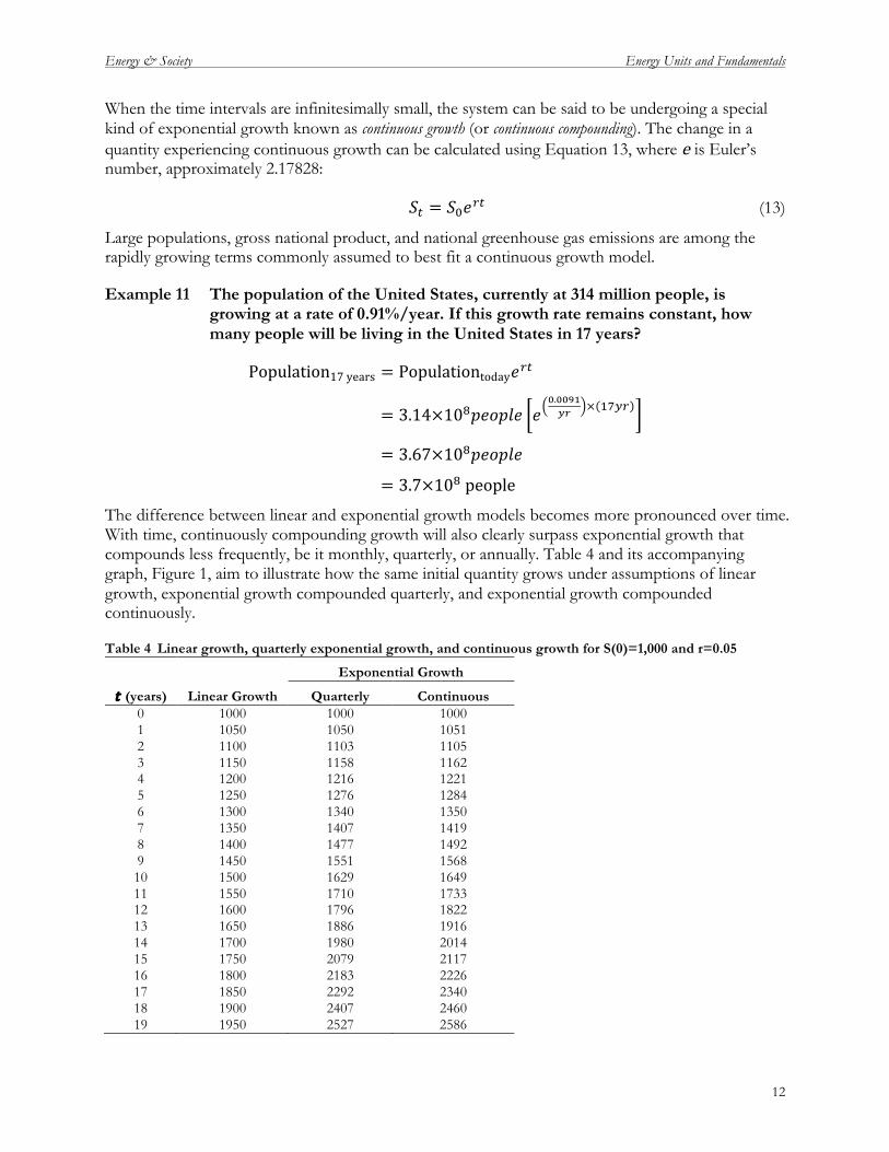
When the time intervals are infinitesimally small, the system can be said to be undergoing a special kind of exponential growth known as continuous growth (or continuous compounding). The change in a quantity experiencing continuous growth can be calculated using Equation 13, where e is Euler’s number, approximately 2.17828:
𝑆! = 𝑆!𝑒!" (13)
Large populations, gross national product, and national greenhouse gas emissions are among the rapidly growing terms commonly assumed to best fit a continuous growth model.
Example 11 The population of the United States, currently at 314 million people, is growing at a rate of 0.91%/year. If this growth rate remains constant, how many people will be living in the United States in 17 years?
Population17 years = Populationtoday𝑒!"
= 3.14×10!𝑝𝑒𝑜𝑝𝑙𝑒 𝑒!.!!"#!" × !"!"
= 3.67×10!𝑝𝑒𝑜𝑝𝑙𝑒
= 3.7×10! people
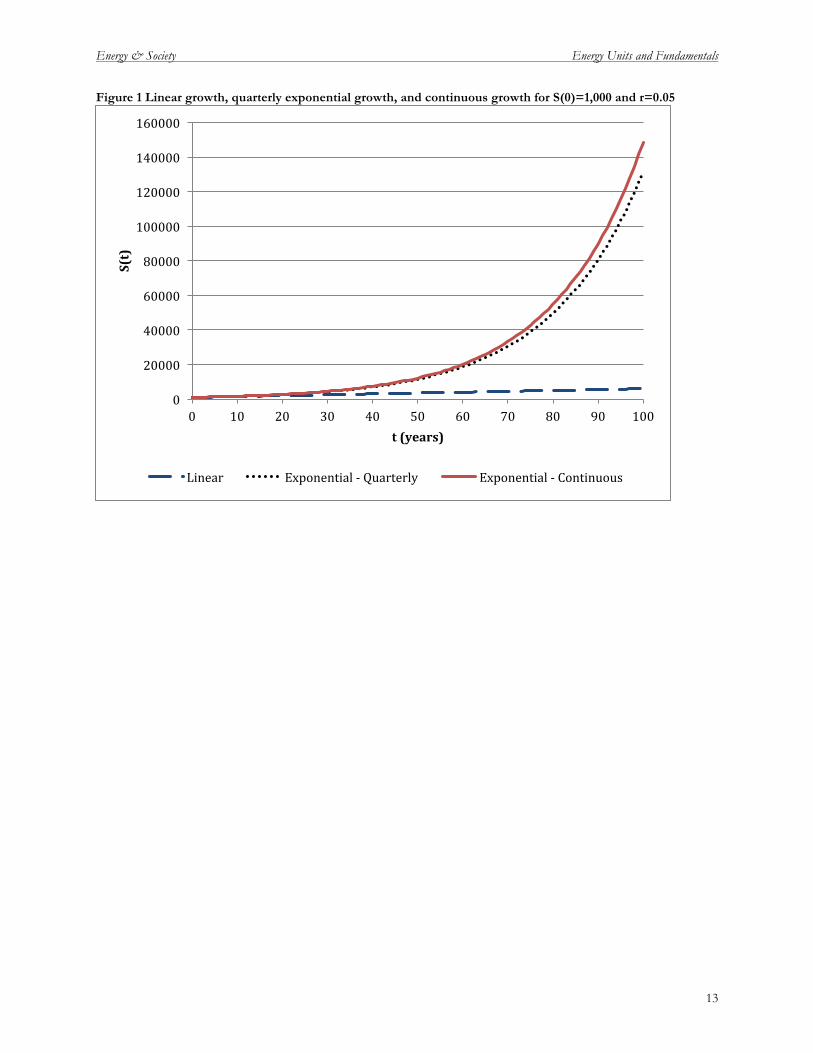
The difference between linear and exponential growth models becomes more pronounced over time. With time, continuously compounding growth will also clearly surpass exponential growth that compounds less frequently, be it monthly, quarterly, or annually. Table 4 and its accompanying graph, Figure 1, aim to illustrate how the same initial quantity grows under assumptions of linear growth, exponential growth compounded quarterly, and exponential growth compounded continuously.
Table 4 Linear growth, quarterly exponential growth, and continuous growth for S(0)=1,000 and r=0.05
t (years) Linear Growth
Exponential Growth
Quarterly Continuous 0 1000 1000 1000 1 1050 1050 1051 2 1100 1103 1105 3 1150 1158 1162 4 1200 1216 1221 5 1250 1276 1284 6 1300 1340 1350 7 1350 1407 1419 8 1400 1477 1492 9 1450 1551 1568 10 1500 1629 1649 11 1550 1710 1733 12 1600 1796 1822 13 1650 1886 1916 14 1700 1980 2014 15 1750 2079 2117 16 1800 2183 2226 17 1850 2292 2340 18 1900 2407 2460 19 1950 2527 2586
Energy & Society Energy Units and Fundamentals
13
Figure 1 Linear growth, quarterly exponential growth, and continuous growth for S(0)=1,000 and r=0.05
0
20000
40000
60000
80000
100000
120000
140000
160000
0 10 20 30 40 50 60 70 80 90 100
S(t)
t (years)
Linear Exponential ‐ Quarterly Exponential ‐ Continuous

Energy & Society Energy Units and Fundamentals
14
4. UNCERTAINTY & SIGNIFICANT FIGURES
From years of basic math training, you know the following to be true:
100𝑔 − 5𝑔 = 95𝑔
What, then, would you say to someone who suggested that in certain circumstances, the following might be more accurate?
100𝑔 − 5𝑔 = 100𝑔
When doing calculations with measurements, you necessarily introduce uncertainty into the problem and must reflect this uncertainty in the answer. In this class, significant figures will provide an indication of the level of accuracy associated with measured values. In the above example, a few steps are skipped in order to get your attention, but these missing steps will be reviewed in the following sections to ensure a full understanding of what significant figures are, how to use them, and why they are important.
4.1. Uncertainty
During your career, you will likely encounter a variety of different conceptions of uncertainty and a corresponding number of techniques to address it. Uncertainty, and efforts to minimize or characterize it, will not be a central focus – as it might be in a data analysis class that uses statistical techniques to calculate how measurement errors (e.g., standard deviations) propagate through an analysis. However, an awareness of uncertainty will be vital for your success in this course as you learn the following skills:
• How to make a reasonable estimate. • How to do back-of-the-envelope calculations and get meaningful answers. • How to improve back-of-the-envelope calculations to get even better answers.
An awareness of uncertainty is necessary to ensure that you do not overstate the accuracy of your results.
Much of the work you will do in this course draws upon data about various types of energy sources, uses, and impacts. These data include, among other things, direct measurements, modeled results, and calculated values. Each of these types of data introduces a degree of uncertainty. When working with these data, it is important to keep in mind that these values have different levels of accuracy associated with them. The accuracy of values can be influenced by instrumentation limits (e.g., a ruler with half-inch marks will allow for less accuracy than a ruler with quarter-inch marks), model errors, natural variation, and human judgment.
In other classes, you might calculate confidence intervals, standard deviations, or other means of representing various types of uncertainty. In this class, we are less concerned about characterizing uncertainty and more concerned about not overstating accuracy. Significant figures provide an indication of the degree of accuracy associated with numerical values.
Energy & Society Energy Units and Fundamentals
15
4.2. Significant Figures
We expect that you will have some familiarity with significant figures from previous courses. The following review is provided as a refresher because you will be expected to use significant figures correctly on problem sets and exams.
Recall that significant figures provide an indication of the degree of accuracy associated with numerical values. Consequently, all measured, modeled, and estimated values have significant figures. Significant figures propagate through calculations according to specific rules. Understanding how significant figures work provides a first-order means for analyzing data: is the accuracy (number of significant figures) of the conclusion supported by the accuracy of the data?
Why does the accuracy of measurements matter? Consider the following example:
Your mom wants to mail you a care package of homemade cookies. The post office calculates postage by the ounce (16 ounces = 1 pound). Therefore, your mom needs to weigh the package in order to determine the correct postage. She first sets the package on the digital bathroom scale. The scale reads: 2 pounds.
If your mom puts on enough postage for 2 pounds, will you receive your cookies?
Maybe.
Remember, the post office calculates postage by the ounce. Luckily for you, your mom is thinking about these issues and is ‘uncertainty savvy’. She looks on the bottom of the scale and finds that its measurements are accurate plus or minus a pound. Although the scale reads 2 pounds, the package could weigh anywhere between 1 and 3 pounds. To guarantee that you get your cookies, a more accurate scale is needed.
Your mom takes the package to the post office and weighs it on a scale accurate to the hundredths place. The scale reads: 2.50 pounds (or 2 pounds 8 ounces). The weight measured by the bathroom scale was not “wrong,” but it was insufficiently accurate to ensure that your cookies get delivered. With the more accurate information provided by the post office scale, your mom is able to apply the appropriate amount of postage, and you get to eat your favorite cookies.
The digital bathroom scale provided a measurement with only one significant figure. The post office scale provided a measurement with three significant figures. For you to get your cookies, your mom needed to rely on the more accurate value.
Thus, significant figures provide an indicator of accuracy for approximate values: the greater the number of significant figures, the greater the accuracy of the value.
4.3. Exact Numbers
Of course, it is important to keep in mind that some values are known with complete certainty. These are known as exact numbers. In this course, most of the exact numbers that you work with will be conversion factors with specific, defined values, e.g., 24 hours per day. Counts of discrete objects, e.g., the number of people in a room, are also exact numbers.
Energy & Society Energy Units and Fundamentals
16
4.4. Identifying Significant Figures
You should be able to identify the number of significant figures a particular measured (or in our case modeled or estimated) value has using a few simple rules:
1. All non-zero digits are significant.
54.3 g has 3 significant figures 54.321 g has 5 significant figures
2. Zeroes between non-zero digits are significant.
1001 kWh has 4 significant figures 2.06 kWh has 3 significant figures
3. Leading zeroes to the left of the first non-zero digit are not significant.
0.0000002 kg has 1 significant figure 0.00607 kg has 3 significant figures
4. Trailing zeroes to the right of a decimal point are significant.
0.0980 cal has 3 significant figures 2.10×10³ cal has 3 significant figures
5. Trailing zeroes to the left of a decimal point are not necessarily significant.
100 toe could have 1, 2, or 3 significant figures, often denoted, 100 (1 sig. figure), or 100.0 (3 significant) figures) 105,000 toe could have 3, 4, 5, or 6 significant figures
Rule 5 introduces a degree of ambiguity into identifying the number of significant figures associated with a particular value. Scientific notation provides an easy way to avoid confusion about the intended number of significant figures. For example, if written in scientific notation, the number of significant figures associated with 105,000,000 could be made clear:
1.05×10⁸ J has 3 significant figures 1.050×10⁸ J has 4 significant figures 1.05000000×10⁸ J has 9 significant figures
Additionally, if a decimal point is placed to the left of trailing zeroes and no digits follow to the right of the decimal point, this indicates that a value is significant to the ones place, thus:
1,000 mL has 1, 2, 3, or 4 significant figures 1,000. mL has 4 significant figures
Energy & Society Energy Units and Fundamentals
17
This convention may be useful in certain circumstances, but we recommend using scientific notation to convey clearly the number of significant figures associated with a particular value.
For problem sets or exams, values with an ambiguous number of significant figures should be assumed to have the fewest significant figures possible:
100 MW should be assumed to have 1 significant figure 250 MW should be assumed to have 2 significant figures
4.5. Rules for Calculations
Different mathematical operations have different rules for how to handle significant figures. These rules are reviewed below. Final answers with a greater number of significant figures than the accuracy of the input information is not correct. The simplest rule is to round results to match the minimum number of significant figures of the information provided to answer the question. Only final answers should be rounded to avoid inaccuracies being introduced by rounding during intermediate steps.
When doing calculations, the accuracy of the calculated value is limited by the accuracy of the
least accurate measurement used in the calculation.
Exact numbers are treated as though they have an infinite number of significant figures and, thus, do not affect the final number of significant figures.
4.5.1. Addition & Subtraction When adding and subtracting values with significant figures, the final answer can have no more decimal places than the value with fewest number of significant figures.
Example 12 100𝑔 − 5𝑔 = 95𝑔
= 100𝑔
= 1×10!𝑔
In Example 12, 100g is the constraining value, accurate only to the hundreds place. The calculated answer shows significant figures to the ones place, so it is necessary to round to the hundreds place. Since the resulting answer has ambiguous significant figures, the final step is to convert the value to scientific notation to make the number significant figures clear.
Now consider a modified version of this problem.
Example 13 101𝑔 − 5𝑔 = 96𝑔
In this example, 5g is the constraining value, since it has the fewest number of significant figures. This constraining value is accurate to the ones place, so in this case, no rounding is necessary.

Energy & Society Energy Units and Fundamentals
18
4.5.2. Multiplication, Division & Exponentiation When multiplying, dividing, or applying exponents with significant figures the final answer can have no more significant figures than the value with the fewest number of significant figures.
Example 14 2.50𝑘𝑚 × 51𝑘𝑚 = 127.5𝑘𝑚
= 130𝑘𝑚
= 1.3×10!𝑘𝑚
In Example 14, 51km is the constraining value with 2 significant figures. The calculated answer shows 4 significant figures and needs to be rounded to only 2 significant figures.
Energy & Society Energy Units and Fundamentals
19
5. UNIT ANALYSIS
Perhaps the single most important problem solving skill for this course is unit analysis. In energy analysis, as in physics (which also aims to describe the physical world with a consistent analytic language), unit analysis provides the basis for a reductionist understanding of the interdependence of the various components of a system. This interdependence implies that understanding the relevant units of measurement in a given system allows one to further understand how changes in the value of any particular unit will affect the other parts of the system. As the Nobel Prize winning physicist Hans Bethe would call out to every student at the blackboard, “slow down, take a breath, and tell me vat are the units? Tell me the units and you will know what you must know to solve the problem.”
Unit analysis – also known as dimensional analysis, factor-label method, or the unit-factor method – is essentially a problem-solving method that uses units to guide mathematical operations.
You have likely encountered unit analysis previously: simple examples include converting inches to centimeters, minutes to hours, or quarters to dollars. In earlier classes when your instructors encouraged you to “check your units,” you were also doing dimensional analysis. In this course, you will use dimensional analysis for converting units, solving more complex problems, and – of course – checking your work.
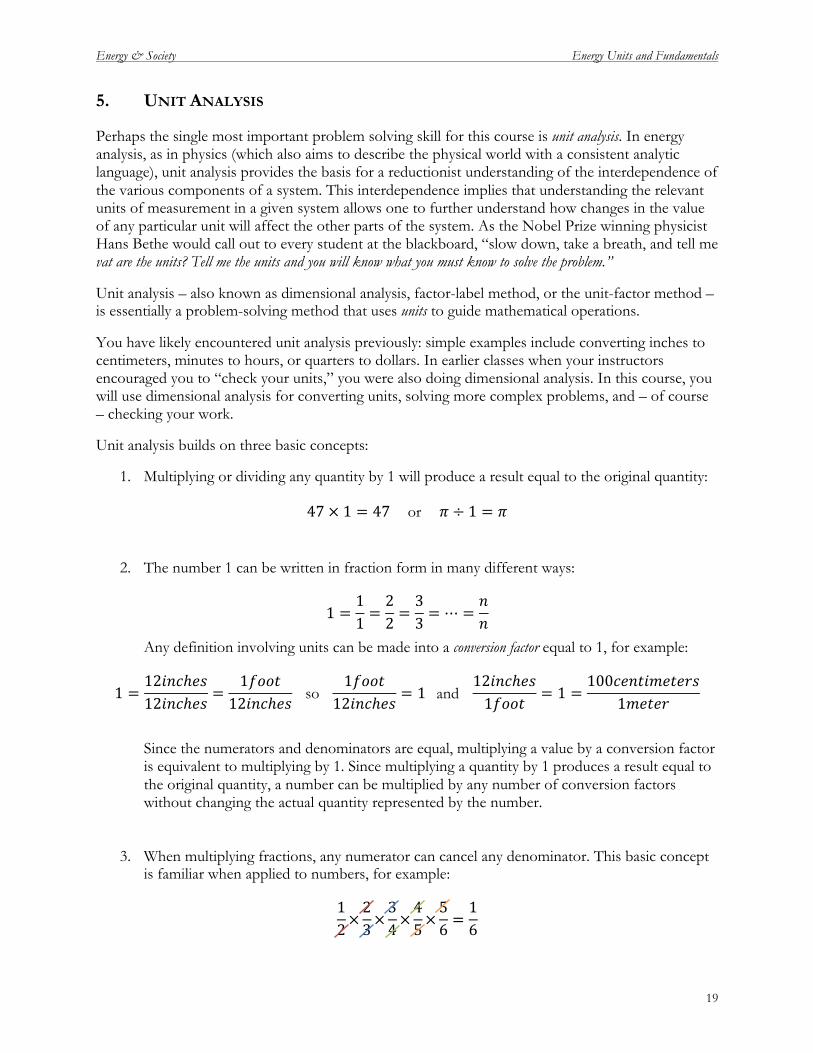
Unit analysis builds on three basic concepts:
1. Multiplying or dividing any quantity by 1 will produce a result equal to the original quantity:
47 × 1 = 47 or 𝜋 ÷ 1 = 𝜋
2. The number 1 can be written in fraction form in many different ways:
1 =11 =
22 =
33 = ⋯ =
𝑛𝑛
Any definition involving units can be made into a conversion factor equal to 1, for example:
1 =12𝑖𝑛𝑐ℎ𝑒𝑠12𝑖𝑛𝑐ℎ𝑒𝑠 =
1𝑓𝑜𝑜𝑡12𝑖𝑛𝑐ℎ𝑒𝑠 so
1𝑓𝑜𝑜𝑡12𝑖𝑛𝑐ℎ𝑒𝑠 = 1 and
12𝑖𝑛𝑐ℎ𝑒𝑠1𝑓𝑜𝑜𝑡 = 1 =
100𝑐𝑒𝑛𝑡𝑖𝑚𝑒𝑡𝑒𝑟𝑠1𝑚𝑒𝑡𝑒𝑟
Since the numerators and denominators are equal, multiplying a value by a conversion factor is equivalent to multiplying by 1. Since multiplying a quantity by 1 produces a result equal to the original quantity, a number can be multiplied by any number of conversion factors without changing the actual quantity represented by the number.
3. When multiplying fractions, any numerator can cancel any denominator. This basic concept is familiar when applied to numbers, for example:
12×
23×
34×
45×
56 =
16
Energy & Society Energy Units and Fundamentals
20
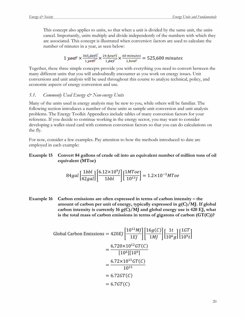
This concept also applies to units, so that when a unit is divided by the same unit, the units cancel. Importantly, units multiply and divide independently of the numbers with which they are associated. This concept is illustrated when conversion factors are used to calculate the number of minutes in a year, as seen below:
1 𝑦𝑒𝑎𝑟 × !"# !"#$! !"#$
× !" !!"#$! !"#
× !" !"#$%&'! !!"#
= 525,600 𝑚𝑖𝑛𝑢𝑡𝑒𝑠
Together, these three simple concepts provide you with everything you need to convert between the many different units that you will undoubtedly encounter as you work on energy issues. Unit conversions and unit analysis will be used throughout this course to analyze technical, policy, and economic aspects of energy conversion and use.
5.1. Commonly Used Energy & Non-energy Units
Many of the units used in energy analysis may be new to you, while others will be familiar. The following section introduces a number of these units as sample unit conversion and unit analysis problems. The Energy Toolkit Appendices include tables of many conversion factors for your reference. If you decide to continue working in the energy sector, you may want to consider developing a wallet-sized card with common conversion factors so that you can do calculations on the fly.
For now, consider a few examples. Pay attention to how the methods introduced to date are employed in each example:
Example 15 Convert 84 gallons of crude oil into an equivalent number of million tons of oil equivalent (MToe)
84𝑔𝑎𝑙1𝑏𝑏𝑙42𝑔𝑎𝑙
6.12×10!𝐽1𝑏𝑏𝑙
1𝑀𝑇𝑜𝑒10!"𝐽 = 1.2×10!!𝑀𝑇𝑜𝑒
Example 16 Carbon emissions are often expressed in terms of carbon intensity – the amount of carbon per unit of energy, typically expressed in g(C)/MJ. If global carbon intensity is currently 16 g(C)/MJ and global energy use is 420 EJ, what is the total mass of carbon emissions in terms of gigatons of carbon (GT(C))?
Global Carbon Emissions = 420𝐸𝐽10!"𝑀𝐽1𝐸𝐽
16𝑔 𝐶1𝑀𝐽
1𝑡10!𝑔
1𝐺𝑇10!𝑡
=6,720×10!"𝐺𝑇 𝐶
10! 10!
=6.72×10!"𝐺𝑇 𝐶
10!"
= 6.72𝐺𝑇 𝐶
= 6.7𝐺𝑇(𝐶)

Energy & Society Energy Units and Fundamentals
21
5.2. Form & Function
One of the features that I hope you will notice in this section is that the equations are very neatly presented. This involves lining up “=” signs, keeping your work in as orderly a form as possible, and keeping all the analysis in the form of symbols to clarify the relationships until the final step of inserting the values to obtain a numeric result.
This is not just a feature of type-set books. As your calculations get more and more complex, you will find that in mathematics neatness truly does count. It is far, far, easier to spot errors, reproduce your results, and as is often the case, to start from one calculation, and build progressively more and more complex models. As in the cartoon below, attention to order and clarity of presentation in your analysis will help you avoid having to search blindly for errors, or justifications for steps that are not obvious, because you will have laid them out clearly as you go. More than one calculation that seemed brilliant at 4 AM, when scratched onto a bit of scrap paper did not hold up to the clear light of day and a more careful and organized analysis.
Energy & Society Energy Units and Fundamentals
22
6. SAMPLE PROBLEMS
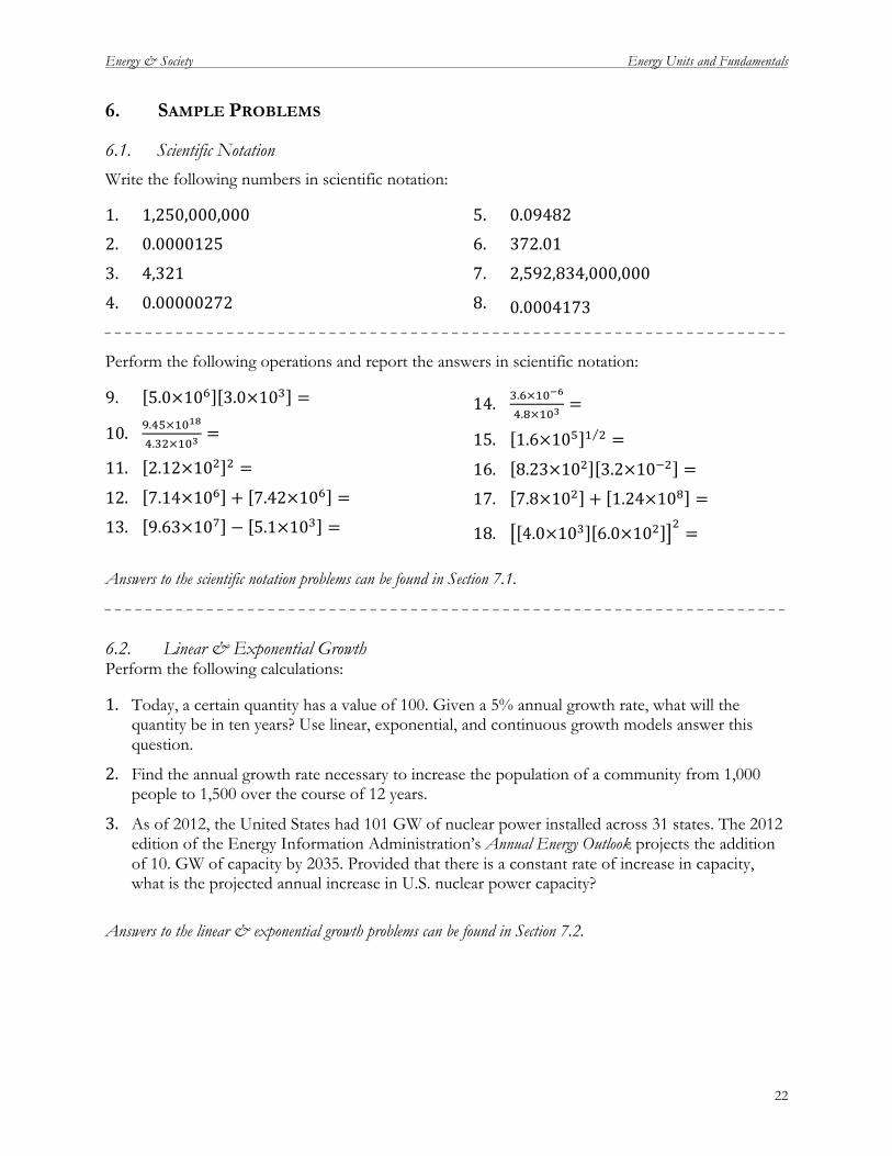
6.1. Scientific Notation
Write the following numbers in scientific notation:
1,250,000,000 1. 0.0000125 2.
4,321 3.
0.00000272 4.
0.09482 5. 372.01 6.
2,592,834,000,000 7.
0.0004173 8.
Perform the following operations and report the answers in scientific notation:
5.0×10! 3.0×10! = 9.
!.!"×!"!"
!.!"×!"!= 10.
2.12×10! ! = 11.
7.14×10! + 7.42×10! = 12.
9.63×10! − 5.1×10! = 13.
!.!×!"!!
!.!×!"!= 14.
1.6×10! ! ! = 15.
8.23×10! 3.2×10!! = 16.
7.8×10! + 1.24×10! = 17.
4.0×10! 6.0×10! ! =18. Answers to the scientific notation problems can be found in Section 7.1.
6.2. Linear & Exponential Growth Perform the following calculations:
1. Today, a certain quantity has a value of 100. Given a 5% annual growth rate, what will the quantity be in ten years? Use linear, exponential, and continuous growth models answer this question.
2. Find the annual growth rate necessary to increase the population of a community from 1,000 people to 1,500 over the course of 12 years.
3. As of 2012, the United States had 101 GW of nuclear power installed across 31 states. The 2012 edition of the Energy Information Administration’s Annual Energy Outlook projects the addition of 10. GW of capacity by 2035. Provided that there is a constant rate of increase in capacity, what is the projected annual increase in U.S. nuclear power capacity?
Answers to the linear & exponential growth problems can be found in Section 7.2.
Energy & Society Energy Units and Fundamentals
23
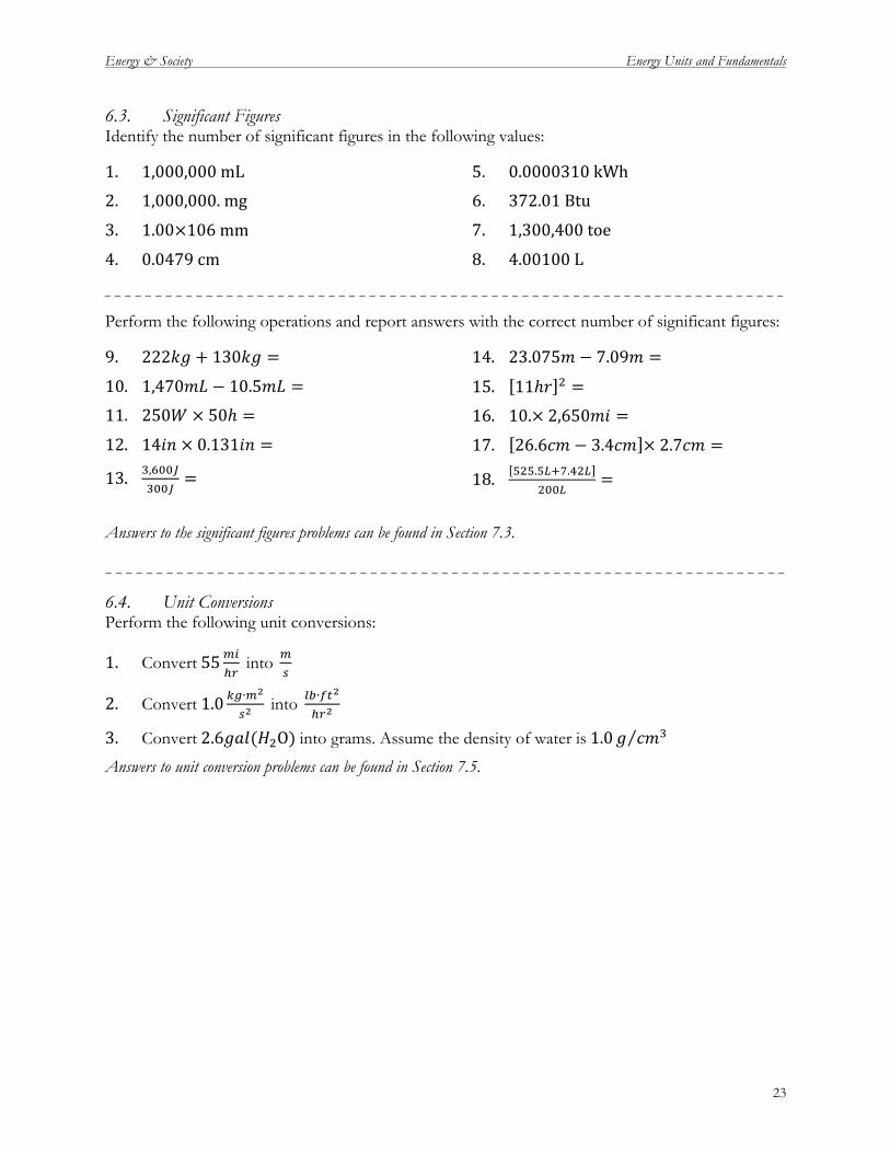
6.3. Significant Figures Identify the number of significant figures in the following values:
1,000,000 mL 1. 1,000,000. mg 2.
1.00×106 mm 3.
0.0479 cm 4.
0.0000310 kWh 5. 372.01 Btu 6.
1,300,400 toe 7.
4.00100 L8.
Perform the following operations and report answers with the correct number of significant figures:
222𝑘𝑔 + 130𝑘𝑔 = 9.
1,470𝑚𝐿 − 10.5𝑚𝐿 = 10. 250𝑊 × 50ℎ = 11.
14𝑖𝑛 × 0.131𝑖𝑛 = 12.
!,!""!!""!
= 13.
23.075𝑚 − 7.09𝑚 = 14.
11ℎ𝑟 ! = 15. 10.× 2,650𝑚𝑖 = 16.
26.6𝑐𝑚 − 3.4𝑐𝑚 × 2.7𝑐𝑚 = 17.
!"!.!!!!.!"!!""!
= 18.
Answers to the significant figures problems can be found in Section 7.3.
6.4. Unit Conversions Perform the following unit conversions:
Convert 55!"!! into !
! 1.
Convert 1.0 !"∙!!
!! into !"∙!"
!
!!! 2.
Convert 2.6𝑔𝑎𝑙(𝐻!O) into grams. Assume the density of water is 1.0𝑔 𝑐𝑚! 3.Answers to unit conversion problems can be found in Section 7.5.
Energy & Society Energy Units and Fundamentals
24
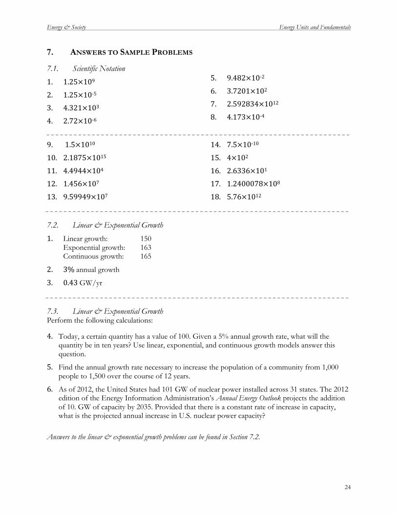
7. ANSWERS TO SAMPLE PROBLEMS
7.1. Scientific Notation
1.25×10⁹ 1.
1.25×10‐5 2. 4.321×10³ 3.
2.72×10‐6 4.
9.482×10‐2 5.
3.7201×10² 6. 2.592834×10¹² 7.
4.173×10‐48.
1.5×10¹⁰ 9.
2.1875×10¹⁵ 10.
4.4944×10⁴ 11. 1.456×10⁷ 12.
9.59949×10⁷ 13.
7.5×10‐10 14.
4×10² 15.
2.6336×101 16. 1.2400078×10⁸ 17.
5.76×101218.
7.2. Linear & Exponential Growth
Linear growth: 150 1.Exponential growth: 163 Continuous growth: 165
3% annual growth 2.
0.43 GW/yr 3.
7.3. Linear & Exponential Growth Perform the following calculations:
4. Today, a certain quantity has a value of 100. Given a 5% annual growth rate, what will the quantity be in ten years? Use linear, exponential, and continuous growth models answer this question.
5. Find the annual growth rate necessary to increase the population of a community from 1,000 people to 1,500 over the course of 12 years.
6. As of 2012, the United States had 101 GW of nuclear power installed across 31 states. The 2012 edition of the Energy Information Administration’s Annual Energy Outlook projects the addition of 10. GW of capacity by 2035. Provided that there is a constant rate of increase in capacity, what is the projected annual increase in U.S. nuclear power capacity?
Answers to the linear & exponential growth problems can be found in Section 7.2.
Energy & Society Energy Units and Fundamentals
23
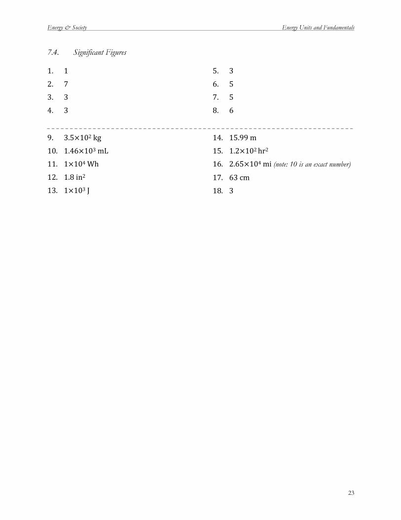
7.4. Significant Figures
1 1.
7 2. 3 3.
3 4.
3 5.
5 6. 5 7.
68.
3.5×10² kg 9.
1.46×10³ mL 10. 1×10⁴ Wh 11.
1.8 in2 12.
1×10³ J 13.
15.99 m 14.
1.2×10² hr2 15. 2.65×10⁴ mi (note: 10 is an exact number) 16.
63 cm 17.
318.

Energy & Society Energy Units and Fundamentals
23
7.5. Unit Conversions
1. 55!"!!
!,!"#!"!!"
!!!.!"!"
!!!!,!""!
= 25!!
2. 1.0 !"∙!!
!!!.!!"!!"
!.!"!"!!
! !"##!!"!
!= 3.1×10! !"∙!"
!
!!!
3. 2.6𝑔𝑎𝑙(𝐻!O)!.!"!!!"#
!,!!!!"!!
!.!!"!
!!"!.!!!!"! = 9.9×10!𝑔

Energy & Society Energy Units and Fundamentals
23
8. REFERENCES
Kammen, Daniel. M. & Hassenzahl, David M. (1999). Should We Risk It: Exploring Environmental Health and Technological Problem Solving. Princeton, NJ: Princeton University Press.
Koomey, Jonathan G. (2001) Turning Numbers into Knowledge: Mastering the Art of Problem Solving (Analytics Press: Oakland, CA).
Smil, Vaclav. (1999). Energies: An Illustrated Guide to the Biosphere and Civilization. Cambridge, MA: MIT Press.
Socolow, Robert, Andrews, Clint A. (1999). Industrial Ecology and Global Change. Cambridge, UK: Cambridge University Press.
Tester, Jefferson, et al. (2005) Sustainable Energy: Choosing Among Options. Cambridge, MA: MIT Press.