Embed Size (px)
Citation preview

1
Energy Profiling and Analysis of the HPC Challenge Benchmarks
Shuaiwen Song1 Rong Ge
2 Xizhou Feng
3 Kirk W. Cameron
4
Abstract
Future high performance systems must use energy efficiently to achieve PFLOPS computational speeds
and beyond. To address this challenge, we must first understand the power and energy characteristics of
high performance computing applications. In this paper, we use a power-performance profiling
framework called PowerPack to study the power and energy profiles of the HPC Challenge benchmarks.
We present detailed experimental results along with in-depth analysis of how each benchmark's workload
characteristics affect power consumption and energy efficiency. This paper summarizes various findings
using the HPC Challenge benchmarks including but not limited to: (1) identifying application power
profiles by function and component in a high performance cluster; (2) correlating application's memory
access patterns to power consumption for these benchmarks; and (3) exploring how energy consumption
scales with system size and workload.
1 Introduction
Today, it is not uncommon for large scale computing systems and data centers to consume massive
amounts of energy, typically 5-10 megawatts in powering and cooling [1]. This results in large electricity
bills and reduced system reliability due to increased heat emissions. The continuing need to increase the
size and scale of these data centers means energy consumption potentially limits future deployments of
high performance computing (HPC) systems.
1 Shuaiwen Song is with the SCAPE Laboratory, Virginia Tech, Blacksburg, VA 24060. Email: [email protected] 2 Rong Ge is with Marquette University, Milwaulkee, WI, 53233. Email: [email protected] 3 Xizhou Feng is with the Virginia Bioinformatics Institute, Virginia Tech, Blacksburg, VA 24060. Email: [email protected] 4 Kirk W. Cameron is with the SCAPE Laboratory, Virginia Tech, Blacksburg, VA 24060. Email: [email protected]

2
Energy efficiency is now a critical consideration for evaluating high performance computing systems. For
example, the Green500 list [2] was launched in November 2006 to rank the energy efficiency of world-
wide supercomputer installations. Meanwhile, the TOP500 supercomputing list, which ranks the most
powerful supercomputing installations has also started to report total power consumption of its
supercomputers [3].
Today, there is no clear consensus as to which benchmark is most appropriate for evaluating the energy
efficiency of high-performance systems. Both the Green500 and the Top500 use the LINPACK [4]
benchmark in their evaluations. In both cases, LINPACK was chosen more for reporting popularity than
its ability to evaluate energy efficiency. As with most benchmark activities, many high-performance
computing stakeholders do not agree with the choice of LINPACK as an energy efficiency benchmark.
Despite the gaining importance of energy efficiency and the controversy surrounding the need for
standardized metrics, there have been few studies detailing the energy efficiency of high-performance
applications. Understanding where and how power is consumed for benchmarks used in acquisition is the
first step towards effectively tracking energy efficiency in high-performance systems and ultimately
determining the most appropriate benchmark. The only detailed HPC energy efficiency study to date has
been for the NAS parallel benchmarks [5].
While both the NAS benchmarks and LINPACK are widely used, the HPC Challenge (HPCC)
benchmarks [6] were specifically designed to cover aspects of application and system design ignored by
the former benchmarks and aid in system procurements and evaluations. HPCC is a benchmark suite
developed by the DARPA High Productivity Computing System (HPCS) program. HPCC consists of
seven benchmarks; each focuses on a different part of the extended memory hierarchy. The HPCC
benchmark provides a comprehensive view of a system's performance bounds for real applications.
A detailed study of the energy efficiency of the HPCC benchmarks is crucial to understand the energy
boundaries and trends of HPC systems. In this paper, we present an in-depth experimental study of the

3
power and energy profiles for the HPC Challenge benchmarks on real systems. We use the PowerPack
toolkit [5, 7] for power-performance profiling and data analysis at function and component level in a
parallel system. This work results in several new findings:
The HPCC benchmark not only provides performance bounds for real applications, but also
provides boundaries and reveals some general trends for application energy consumption.
Each HPCC application has its own unique power profiles and such profiles vary with runtime
settings and system configurations.
An application’s memory access rate and locality strongly correlate to power consumption.
Higher memory access locality is indicative of higher power consumption.
System idle power contributes to energy inefficiency. Lower system idling power would
significantly increase energy efficiency for some applications.
The rest of the paper is organized as follows. Section 2 discusses related work. Section 3 reviews
PowerPack and the HPCC benchmarks. Section 4 and 5 present an in-depth examination and analysis of
the power and energy profiles of the HPCC benchmarks. Section 6 summarizes our conclusions and
highlights future research directions.
2 Related Work
HPC researchers and users have begun measuring and reporting the energy efficiency of large scale
computer systems. Green500 [8], TOP500 [3] and SPECPower [9] provide methodologies and public
repositories for tracking total system-wide power and efficiency. HPC systems contain a diverse number
and type of components including processors, memory, disks, and network cards at extreme scales.
Understanding the energy scalability of an HPC system thus requires tracking the energy efficiency of the
entire system as well as each component within the system at scale. However, all of the aforementioned

4
methodologies and lists consider only the aggregate power of an entire system lacking critical details as to
the proportional energy consumption of individual components.
Most early power measurement studies focused on system or building level power [10] measured with
proprietary hardware [11], through power panels, or empirical estimations using rules-of-thumb [12]. The
first detailed energy study of HPC applications [5] confirmed power profiles of the NAS parallel
benchmarks at the system level corresponded to performance related activity such as memory accesses.
These results were later confirmed in a study [13] that additionally measured high-performance
LINPACK (HPL) on a number of systems.
In previous work [5], we developed a software/hardware toolkit called PowerPack and used it to evaluate
the power profiles and energy efficiency for various benchmarks including the entire NPB benchmark
suite on several high-performance clusters. PowerPack provides the infrastructure and methodology for
power and performance data logging, correlation of data to source code, and post processing of the data
collected for the benchmark under study. In addition to the software framework, PowerPack requires
power measurement hardware to obtain direct measurements of the entire system and each component.
We use a direct measurement methodology for capturing performance and power data. There have been
other efforts to capture HPC energy efficiency analytically [14-16]. For example, the Power-aware
Speedup model was proposed [14] to generalize Amdahl’s law for energy. Another approach was
proposed to study the energy implications of multicore architectures [15]. PowerPack provides direct
measurement since we are interested in profiling the impact of energy consumption on HPC systems and
applications. These analytical approaches are appropriate for further analyses using the data provided by
tools such as PowerPack.
In this work, we study component and function level power consumption details for the HPCC
benchmarks on advanced multicore architectures. The HPCC benchmarks were chosen since they were
designed to explore the performance boundaries of current systems. Some results, such as the high-

5
performance LINPACK portion of the HPCC suite, have appeared in aggregate total system form in the
literature, but not at function and component level granularity. Other portions of the suite, such as
STREAM, have not been profiled for power previously at this level of detail to the best of our knowledge.
Since the HPCC benchmarks collectively test the critical performance aspects of a machine, we study in
this work whether these benchmarks also examine the critical energy aspects of a system.
3 Descriptions of the Experimental Environment
To detail the power-energy characteristics of the HPCC benchmarks on high performance systems, we
use experimental system investigation. We begin by describing the setup of our experimental environment
which consists of three parts: the PowerPack power-profiling framework, the HPCC benchmark suite, and
the HPC system under test.
3.1 The PowerPack power-profiling framework
PowerPack is a framework for profiling power and energy of parallel applications and systems. It consists
of both hardware for direct power measurement, and software for data collection and processing.
PowerPack has three critical features: 1) direct measurements of the power consumption of a system's
major components (i.e. CPU, memory, and disk) and/or an entire computing unit (i.e. an entire compute
node); 2) automatic logging of power profiles and synchronization to application source code; and 3)
scalability to large scale parallel systems. PowerPack uses direct measurements from power meters to
obtain accurate and reliable power and energy data for parallel applications. The current version of
PowerPack supports multicore multi-processor with dynamic power management configurations.
Figure 1 shows the software architecture of the PowerPack framework. PowerPack consists of five
components: hardware power/energy profiling, software power/energy profiling control, software system
power/energy control, data collection/fusion/analysis, and the system under test. The hardware
power/energy profiling module simultaneously measures system power and multiple components’ power.

6
PowerPack measures the system power using a power meter plugged between the computer power supply
units and electric outlets. Component power is measured using precision resistors inserted into the DC
lines output from the computer's power supply unit and voltage meters attached at two ends of the
resistors. The software power/energy profiling control module provides meter drivers and interface (i.e.
APIs) for the system or an application to start/stop/label power profiling. The software system
power/energy module is a set of interfaces (i.e. APIs) to turn on/off or to set frequencies of processors.
The data fusion module merges multiple data streams and transforms them into a well-structured format.
Normally, PowerPack directly measures one physical node at a time but is scalable to the entire computer
cluster using node remapping and performance counter based analytical power estimations.
3.2 The HPC Challenge benchmark
The HPC Challenge (HPCC) benchmark [6] is a benchmark suite that aims to augment the TOP500 list
and to evaluate the performance of HPC architectures from multiple aspects. HPCC organizes the
benchmarks into four categories; each category represents a type of memory access pattern characterized
by the benchmark's memory access spatial and temporal
locality. Currently, HPCC consists of seven benchmarks:
HPL, STREAM, RandomAccess, PTRANS, FFT, DGEMM
and b_eff Latency/Bandwidth. To better analyze the
power/energy profiles in the next section, we summarize the
memory access patterns and performance bounds of these
benchmarks in Table 1.
We use a classification scheme to separate distinct
performance phases that make up the HPCC benchmark suite. In LOCAL mode, a single processor runs
the benchmark. In STAR mode, all processors run separate independent copies of the benchmark with no
Hardware power/energy profiling
HPC Cluster
Software power/energy control
Data Collection
Figure 1 Power Pack Software Architecture

7
communication. In GLOBAL mode, all processing elements compute the benchmark in parallel using
explicit data communications.
3.3 The HPC system under test
The Dori system is a cluster of nine two-way dual-core AMD Opteron 265 based server nodes. Each node
consists of six 1 GB memory modules, one Western Digital WD800 SATA hard drive, one Tyan Thunder
S2882 motherboard, two CPU fans, two system fans, three Gigabit Ethernet ports, and one Myrinet
interface. The compute nodes run CentOS linux with kernel version 2.6. During our tests, we used
MPICH2 as the communication middleware. The network interconnect is gigabit Ethernet.
4 HPCC Benchmark Power Profiling and Analysis
4.1 A snapshot of the HPCC power profiles
The power profiles of each application are unique. Figure 2 shows power profiles of the HPCC
benchmarks running on two nodes of the Dori cluster. This profile is obtained using the problem size
where HPL achieves its maximum performance on two nodes. Power consumption is tracked for major
computing components including CPU, Memory, Disk and Motherboard. As we will see later, these four
components capture nearly all the dynamic power usage of the system that is dependent on the application.
A single HPCC test run consists of a sequence of eight benchmark tests as follows: (1) Global PTRANS,
Table 1. Performance characteristics of the HPCC Benchmark suite.
Benchmark Spatial
Locality
Temporal
Locality Mode Detail
HPL high high GLOBAL Stresses floating point performance
DGEMM high high STAR+LOCAL Stresses floating point performance
STREAM high low STAR Measures memory bandwidth
PTRANS high low GLOBAL Measures data transfer rate
FFT low high GLOBAL+STAR+LOCAL Measures float point + memory transfer performance
RandomAccess low low GLOBAL+STAR+LOCAL Measures random updates of int memory
Latency/Bandwidth low low GLOBAL Measures latency and bandwidth of comm patterns

8
(2) Global HPL, (3) Star DGEMM + Local DGEMM, (4) Star STREAM, (5) Global MPI RandomAccess,
(6) Star RandomAccess, (7) Local RandomAccess, and (8) Global MPI FFT, Star FFT, Local FFT and
Latency/Bandwidth. Figure 2 clearly shows the unique power signature of each mode of the suite. We
make the following observations from Figure 2:
(1) Each test in the benchmark suite stresses processor and memory power relative to their use. For
example, as Global HPL and Star DGEMM have high temporal and spatial locality, they spend little
time waiting on data and stress the processor's floating point execution units intensively and consume
more processor power than other tests. In contrast, Global MPI RandomAccess has low temporal and
spatial memory access locality, thus this test consumes less processor power due to more memory
access delay, and more memory power due to cache misses.
(2) Changes in processor and memory power profiles correlate to communication to computation ratios.
Power varries for global tests such as PTRAN, HPL, and MPI_FFT because of their computation and
communication phases. For example, HPL computation phases run 50 Watts higher than its
communication phases. Processor power does not vary as much during STAR (embarrassingly
parallel) and LOCAL (sequential) tests due to limited processing variability in the code running on
each core. In GLOBAL modes, memory power varies, but not widely in absolute wattage since
memory power is substantially less than processor power on the system under test.
(3) Disk power and motherboard power are relatively stable over all tests in the benchmarks. None of the
HPCC benchmarks stresses local disks heavily. Thus power variations due to disk are not substantial.
On this system, the network interface card (NIC), and thus its power consumption, is integrated in the
motherboard. Nonetheless, communication using the gigabit Ethernet card does not result in
significant power use even under the most intensive communication phases.

9
(4) Processors consume more power during GLOBAL and STAR tests since they use all processor cores
in the computation. LOCAL tests use only one core per node and thus consume less energy.
4.2 Power distribution among system components
Each code within the HPCC benchmarks is unique in its memory access pattern. Together, they
collectively examine and identify the performance boundaries of a system with various combinations of
high and low temporal and spatial locality, as described in Table 1. We hypothesize that the HPCC
benchmarks will identify analogous boundaries for power and energy in high performance systems and
applications. HPL (high, high), PTRAN (low, high), Star_FFT (high, low) and Star_RandomAccess (low,
low) represent the four combinations of (temporal, spatial) locality captured by the HPCC tests. Figure 3
superimposes the results for these four tests on an X-Y plot of temporal-spatial sensitivity. For
comparison, below the graph we also provide the power breakdowns of system idle (i.e. no active user
applications), and disk copy that stresses disk I/O access which is not captured by the HPCC tests.
Power Prof ile for HPCC benchmarks running on 8 cores of 2 nodes
0
20
40
60
80
100
120
140
160
180
0 351 702 1054 1405 1756 2108 2459 2810 3161 3513 3864
Time (seconds)
Po
we
r (w
att
s)
CPU Memory Disk Mot herboard
1 2 34 5 6 7 8
Figure 2. A snapshot of the HPCC power profile. The power consumption of major components per compute node when
running a full HPCC benchmark suite using eight cores. The entire run of HPCC consists of seven micro benchmark tests in the
order as follows. 1. PTRANS, 2 HPL, 3. Star DGEMM + single DGEMM, 4. Star STREAM, 5. MPI_RandomAccess, 6.
Star_RandomAccess, 7. Single_RandomAccess, 8. MPI_FFT, Star_ FFT, single FFT and latency/bandwidth. In this test, the
problem size fits the peak execution rate for HPL. For LOCAL tests, we run a benchmark on a single core with three idle cores.

10
The total power consumption figures for each of the isolated phases of the HPCC benchmark depicted in
Figure 3 in increasing order are: system idle (157 Watts), disk copy (177 Watts), Star_RandomAccess
(219 Watts), Star_FFT (221 Watts), PTRAN (237 Watts), and HPL (249 Watts). The power numbers for
the two STAR benchmarks are representative given the stable power profiles, while the power numbers
for PTRAN and HPL are of time instances when processor power reaches the respective maximum. We
conclude the following from the data:
Since lower temporal and spatial locality imply higher average memory access delay times,
applications with (low, low) temporal-spatial locality use less power on average. Memory and
processor power dominate the power budget for these codes. Idling of processor during memory
access delays results in more time spent idling at lower dynamic processor power use thus leading
to lower average system power use.
Since higher temporal and spatial locality imply lower average memory access delay times,
applications with (high, high) temporal-spatial locality use more power on average. Memory and
processor power dominate the power budget for these codes. Intensive floating point execution
leads to more activities and higher active processor power and average system power. Since HPL
has both high spatial and temporal locality, it consumes the highest power consumption and thus
is a candidate for measuring the maximum system power an application would require.
Mixed temporal and spatial locality implies mixed results that fall between the average power
ranges of (high, high) and (low, low) temporal-spatial locality codes. These codes must be
analyzed more carefully by phase since communication phases can affect the power profiles
substantially.

11
Overall, processor power dominates total system power for each test shown in Figure 3; the processor
accounts for as little as 44% of the power budget for disk copy and as much as 61% of the power budget
for HPL. Processor power also shows the largest variance as high as 59 Watts for HPL. For workloads
with low temporal and spatial locality, such as Star_RandomAccess, processor power consumption varies
as much as 40 Watts.
S ta rt-F F T (221 Wa tts)
56%
11%
3%
6%
4%
14%
6%
Sp
ati
al L
oc
ali
ty
Temporal Locality
S tar-RandomAc c es s (219 Watts )
52%
14%
4%
6%
4%
14%
6%
P T R ANS (237 Wa tts)
57%
10%
3%
6%
4%
14%
6%
HP L (249 Wa tts)
64%8%
3%
5%
3%
12%5%
low high
low
h
igh
S ystem Idle (157 Wa tts)
49%
11%4%
8%
5%
15%
8%
Disk C opy (177 Wa tts)
44%
10%11%
7%
5%
16%
7%
Figure 3. System power distribution for different workload categories. This figure shows system power broken down by
component for six workload categories. The top four categories represent four different memory access locality patterns. The
other two workloads are system idle, i.e., no user application running, and disk copy, i.e., concurrently running the Linux
standard copy program on all cores. The number included in the subfigure title is the total average power consumption.

12
Memory is the second largest power consumer in the HPCC tests and accounts for 8% (HPL) and 13%
(RandomAccess) of total system power consumption. Low spatial locality causes additional memory
accesses and thus higher memory power consumption. For Star_RandomAccess, the memory power
increases by 11 Watts over the idle system.
Disk normally consumes much less power than processor and memory, but may consume up to 11% of
total system power for disk I/O intensive applications like disk copy. Few HPC benchmarks, including
HPCC, LINPACK, and the NAS parallel benchmarks stress disk accesses. This may be due to the fact
that in high performance environments with large storage needs, data storage is remote to the
computational nodes in a disk array or other data appliance. We use the disk copy benchmark to primarily
illustrate how the power budget can change under certain types of loads meaning local disk power should
not be readily dismissed for real applications.
The system under test consumes a considerable amount of power when there is no workload running. We
have omitted discussion of power supply inefficiency since it is fundamentally an electrical engineering
problem which accounts for another 20-30% of the total system power consumed under these workloads.
Altogether, the processor, the power supply, and the memory are the top three power consuming
components for the HPCC benchmarks and typically account for about 70% of total system power.
4.3 Detailed power profiling and analysis of Global HPCC tests
The previous subsection is focused on the effect of memory access localities of applications on power
distribution over the system components. In this section, we study how parallel computation changes the
locality of data accesses and impacts the major computing components’ power profiles over benchmarks’
executions. We still use the same four benchmarks, all of them in GLOBAL mode.
PTRANS implements a parallel matrix transpose. HPCC uses PTRANS to test system communication
capacity using simultaneous large message exchanges between pairs of processors. Figure 4(a) shows the

13
power profiles of PTRANS with problem size N=15000. Processor power varies within iterations. The
spikes correspond to computation phases and valleys correspond to system-wide large message exchanges
which occur on iteration boundaries as marked in the figure. While PTRANS’s power consumption is
reasonably high during computation phases, its power consumption during communication phases is close
to the lowest. Also, the memory power profile is stable with only slight changes. PTRANS has high
spatial locality and consequently a low cache miss rate. Communication phases are sufficiently long
enough for the processor to reduce its power consumption. Additionally the computation phases of
PTRANS focus on data movement to perform the transpose which is less computationally intensive than
the matrix computations in HPL, which results in a lower average power consumption for PTRANS
computation phases.
HPL is a computation intensive workload interspersed with short communications. HPCC uses HPL to
assess peak floating point performance. HPL’s processor power profiles show high variance, as shown in
Figure 4(b). For this data, we experimentally determined a problem size where HPL achieves peak
execution rate on 32 cores across 8 nodes. At peak HPL performance, processor power reaches about 150
Watts, which is the maximum over all HPCC tests. Nevertheless, processor power fluctuates dramatically.
Processor power may drop to 90 Watts during the short communications in HPL. Memory power does not
vary much during HPL execution. This is because HPL has high temporal and spatial memory access
locality, and thus does not frequently incur cache misses.
MPI_RandomAccess is a GLOBAL test that measures the rate of integer updates to random remote
memory locations. This code’s memory access pattern has low spatial and temporal locality. As shown in
Figure 4(c), the processor power profile for MPI_RandomAccess follows a steady step function that
reflects the relatively low computational intensity of random index generation. MPI_RandomAccess
stresses inter-processor communication of small messages. Processor power decreases during the message
exchange of indices with other processors. Memory power jumps towards the end of the run as the local

14
memory updates occur once all indices are received. This memory power consumption is notably almost
the highest among all the GLOBAL tests. The only higher memory power consumption we observed was
for the EP (Embarrassingly parallel) version of this code, Star_RandomAccess.
MPI_FFT is a GLOBAL test that performs the fast Fourier transform operation. Figure 4(d) shows the
power profiles of MPI_FFT with input vector size of 33,554,432. MPI_FFTs processor power profile is
similar to that of PTRANS in which communication tends to decrease processor power on function
boundaries as marked in the figure. Unlike PTRANS however, the memory power profile of MPI_FFT
PTRANS
0
20
40
60
80
100
120
140
6 7 8 9 10 11 13 14 15 16
Timestamp (seconds)
Po
wer
(watt
s)
CPU Memory
Hard disk Motherboard
it er 2it er 1 it er 3 it er 4
HPL
0
20
40
60
80
100
120
140
160
180
0 234 469 703 937 1172 1406 1641 1875 2109 2344
Time (seconds)
Po
wer
(watt
s)
CPU Memory Disk Motherboard
(a) (b)
MPI_RandomAccess
0102030405060708090
100
0 47 94 140 187 234 281 328 375 421Time (seconds)
Po
wer
(watt
s)
CPU MemoryDisk Motherboard
MPI_FFT
0
20
40
60
80
100
120
4 6 7 9 11 13 15 17 19 21
Time (seconds)
Po
wer
(watt
s)
CPU Memory
Hard disk Motherboard
(c) (d) Figure 4. Detailed power profiles of four HPCC benchmarks running across 8 nodes on 32 cores in GLOBAL mode. This figure shows the power consumptions of system major components over time for (a)PTRANS, (b)HPL, (c)
MPI_RandomAccess, and (d) MPI_FFT during their entire execution.
15
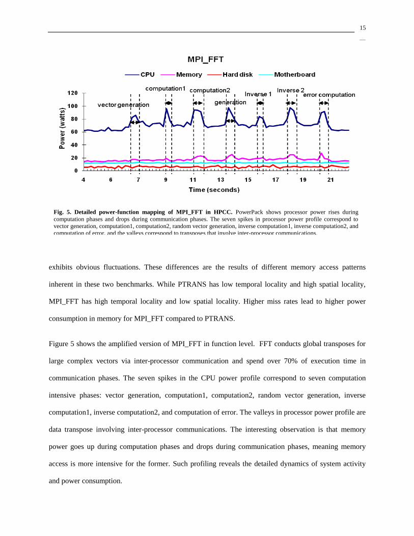
exhibits obvious fluctuations. These differences are the results of different memory access patterns
inherent in these two benchmarks. While PTRANS has low temporal locality and high spatial locality,
MPI_FFT has high temporal locality and low spatial locality. Higher miss rates lead to higher power
consumption in memory for MPI_FFT compared to PTRANS.
Figure 5 shows the amplified version of MPI_FFT in function level. FFT conducts global transposes for
large complex vectors via inter-processor communication and spend over 70% of execution time in
communication phases. The seven spikes in the CPU power profile correspond to seven computation
intensive phases: vector generation, computation1, computation2, random vector generation, inverse
computation1, inverse computation2, and computation of error. The valleys in processor power profile are
data transpose involving inter-processor communications. The interesting observation is that memory
power goes up during computation phases and drops during communication phases, meaning memory
access is more intensive for the former. Such profiling reveals the detailed dynamics of system activity
and power consumption.
Fig. 5. Detailed power-function mapping of MPI_FFT in HPCC. PowerPack shows processor power rises during
computation phases and drops during communication phases. The seven spikes in processor power profile correspond to
vector generation, computation1, computation2, random vector generation, inverse computation1, inverse computation2, and
computation of error, and the valleys correspond to transposes that involve inter-processor communications.

16
5 HPCC Benchmark Energy Profiling and Analysis
While we are interested in power (P), the rate of energy consumption at time instances when an
application executes, we are also interested in system energy consumption (E) required to finish executing
the application. Energy is the area under the curves given by the power profiles previously discussed. It
reflects the electrical cost of running an application on a particular system. In this section we analyze the
resulting impact of power profiles on energy consumption on parallel systems. In particular we study the
energy efficiency of these applications and systems as they scale.
5.1 Energy profiling and efficiency of MPI_FFT under strong scaling
Strong scaling describes the process of fixing a workload and scaling up the number of processors.
Embarrassingly parallel codes often scale well under strong scaling conditions. For these types of codes,
scaling system size reduces execution times linearly with constant nodal power consumption. As a result,
the total energy consumption maintains the same. When measuring energy efficiency with the amount of
workload computed per unit of energy, an embarrassingly parallel code achieves better energy efficiency
as system size scales.
However, for codes that are not embarrassingly parallel, such as Global MPI_FFT, the energy efficiency
is less clear. In Figure 6, we show the power per node, system energy, performance, and resulting energy
efficiency of a set of Global MPI_FFT tests. Using a fixed problem size that is same as the one mentioned
in Section 4.3, we run MPI_FFT at different numbers of nodes. During the test, we use all the four cores
on each node. Thus, running on 8 nodes actually creates 32 threads with one thread per core. Figure 6(a)
shows the components’ power per node. As system size scales, the duration of high processor power
phases (computation phases) becomes shorter, and the duration of lower processor power phases
(communication phases) becomes longer. In addition, the highest processor power within one run slightly
decreases when the number of nodes increases. Memory power also shows a similar trend.

17
Figure 6(b) shows that both performance and energy increase sub-linearly as system size scales. However,
energy increases much faster than performance for the system sizes we have measured. For example,
running on eight nodes gains 2.3 times speedup but costs 3.3 times energy as much as that when running
on one node. This observation implies the need of appropriate tradeoffs between running an application
faster and maintaining sufficient energy efficiency or constraining running cost.
0
20
40
60
80
100
120
Pow
er (W
atts
)
Time (seconds)
Power profiles of MPI_FFT under strong scaling
CPU Memory
1 node 2 nodes 4 nodes 8 nodes
(a)
0.0
0.5
1.0
1.5
2.0
2.5
3.0
3.5
1 2 4 8
No
rmal
ize
d V
alu
es
Number of Nodes
MPI_FFT Energy and Performance Scaling for Fixed Problem Size
Normalized Performance
Normalized Energy
Normalized Performance/Energy
(b)
Figure 6. The power, energy, performance, and energy efficiency of MPI_FFT. In this figure, we run global
MPI_FFT test for a fixed problem size using varying number or nodes with four cores per node. Both performance and
energy are normalized against respective values when using one node. We use normalized performance/energy as a measure
of achieved energy efficiency.
20.1 18.3 14.3 9.1

18
5.2 Energy profiling and efficiency of HPL under weak scaling
Weak scaling describes the process of simultaneously increasing both workload and the number of
processors being used. The discussions on energy efficiency under strong scaling imply that in order to
maintain a desired level of energy efficiency, we also need to maintain the parallel efficiency of the
application. In the experiments below, we want to find out how effectively the weak scaling case can
maintain its parallel and energy efficiency.
Figure 7 shows the directly measured power, energy, performance, and energy efficiency of HPL on Dori
cluster under weak scaling. In our experiments, we increase the problem size of HPL in such a way that
HPL always achieves its maximum performance on the respective number of nodes. Figure 7(a) shows
the power profiles of HPL. With weak scaling, neither processor power nor memory power change
perceivably with the number of nodes during computation phases, though it decreases slightly during
communication phases as system scales. As a result, average nodal power almost remains the same.
Figure 7(b) shows the normalized performance and derived total energy. We observe that both
performance and energy increase rough linearly as system size increases. Accordingly, the energy
efficiency keeps constant as system size increases. These observations exactly match our expectation. By
increasing the problem size of HPL to match the system’s maximum computational power, we maintain
the memory spatial and temporal locality and parallel efficiency, which in turn leads to constant energy
efficiency. We would like to note observations from weak scaling of HPL are very close to that from
embarrassingly parallel.

19
6 Summary and Conclusions
In summary, we evaluated the power and performance profiles of the HPC Challenge benchmark suite on
a multicore based HPC cluster. We used the PowerPack toolkit to collect the power and energy profiles
and isolate them by components. We organized and analyzed the power and energy profiles by each
benchmark's memory access locality.
Each application has a unique power profile characterized by power distribution among major system
components, especially processor and memory, as well as power variations over time. By correlating the
(a)
0
1
2
3
4
5
6
1 2 3 4 5 6
No
rmal
ize
d V
alu
es
Number of Nodes
HPL Energy/Performance Scaling for Scaled Workload
Normalized Performance
Normalized Energy
Normalized Performance/Energy
(b)
Figure 7. The power, energy, performance, and energy efficiency of HPL under weak scaling. In this figure, both
performance and energy are normalized against corresponding values when using one node. We also plot the normalized
performance/energy value as a measure of achieved energy efficiency.
20
HPCC benchmark's power profiles to performance phases, we directly observed strong correlations
between power profiles and memory locality.
The power profiles of the HPCC benchmark suite reveal power boundaries for real applications.
Applications with high spatial and temporal memory access locality consume the most power but achieve
the highest energy efficiency. Applications with low spatial or temporal locality usually consume less
power but also achieve lower energy efficiency.
Energy efficiency is a critical issue in high performance computing that requires further study since the
interactions between hardware and application affect power usage dramatically. For example, for the
same problem on the same HPC system, choosing an appropriate system size will significantly affect the
achieved energy efficiency.
In the future, we will extend the methodologies used in this paper to larger systems and novel
architectures. Additionally, we would like to explore further energy-efficiency models and the insight
they provide to the sustainability of large scale systems.
7 Acknowledgement
This material is based upon work supported by the National Science Foundation under Grant No.
0910784 and 0905187.
REFERENCES
1. Cameron, K.W., R. Ge, and X. Feng, High-performance, Power-aware, Distributed Computing for
Scientific Applications. IEEE Computer, 2005. 38(11): p. 40-47.
2. Feng, W.-C. and K.W. Cameron, The Green500 List: Encouraging Sustainable Supercomputing. IEEE
Computer, 2007. 40(12): p. 50-55.
3. U. of Tennessee, Top 500 Supercomputer list..SC08 conference, Nov. 15-21 in Austin, 2008; Available
from: http://www.top500.org/list/2008/11/100.
4. Dongarra, J., The LINPACK Benchmark: An Explanation. Evaluating Supercomputers: p. 1-21.
5. Feng, X., R. Ge, and K.W. Cameron. Power and Energy Profiling of Scientific Applications on Distributed
Systems (IPDPS 05). in 19th IEEE International Parallel and Distributed Processing Symposium. 2005.
Denver, CO.

21
6. Luszczek, P., et al., Introduction to the HPC Challenge Benchmark Suite. SC2005 (submitted), Seattle, WA,
2005.
7. Cameron, K., R. Ge, and X. Feng, High-performance, power-aware distributed computing for scientific
applications. Computer, 2005. 38(11): p. 40-47.
8. Feng, W. and K. Cameron, The Green500 List: Encouraging Sustainable Supercomputing. Computer, 2007.
40(12): p. 50-55.
9. SPEC, The SPEC Power Benchmark. 2008, website: http://www.spec.org/power_ssj2008/.
10. LBNL, Data Center Energy Benchmarking Case Study: Data Center Facility 5. 2003.
11. IBM. PowerExecutive. 2007, website: http://www-03.ibm.com/systems/management/director/extensions/
powerexec.html.
12. Bailey, A.M., Accelerated Strategic Computing Initiative (ASCI): Driving the need for the Terascale
Simulation Facility (TSF), in Energy 2002 Workshop and Exposition. 2002: Palm Springs, CA.
13. Shoaib, K., J. Shalf, and E. Strohmaier, Power Efficiency in High Performance Computing, in High-
performance, power-aware computing workshop. 2008: Miami, FL.
14. Ge, R. and K. Cameron. Power-aware speedup. Parallel and Distributed Processing Symposium,
IPDPS ,2007.
15. Cho, S. and R. Melhem, Corollaries to Amdahl's Law for Energy. Computer Architecture Letters, 2008.
7(1): p. 25-28.
16. Yang Ding; Malkowski, K, Raghavan, P, Kandemir, M. Towards energy efficient scaling of scientific codes.
Parallel and Distributed Processing, 2008. April 2008.