Embed Size (px)
Citation preview

ENERGY PERFORMANCE
ESTIMATION OF COOLING TOWERS
by
ZILAI ZHAO
KEITH WOODBURY, COMMITTEE CHAIR
ZHENG O’NEILL
ROBERT BATSON
A THESIS
Submitted in partial fulfillment of the requirements
for the degree of Master of Science
in the Department of Mechanical Engineering
in the Graduate School of
The University of Alabama
TUSCALOOSA, ALABAMA
2016

Copyright Zilai Zhao 2016
ALL RIGHTS RESERVED

ii
ABSTRACT
The goal of this project is to investigate and compare the performance of cooling
towers using Effectiveness-NTU model and empirical model. The processes to achieve the
goal include: Developed Effectiveness-NTU and empirical models of the cooling tower, and
predicted the performance of the design and off-design conditions; Stated experimental
protocols and gathered data on the HVAC cooling tower on the campus of the University of
Alabama; Used collected data to validate the models; Compared results from models with
real measurements and found the limitation of each model; Applied known annual weather
data to estimate the performance and energy consumption of the cooling tower;
Recommended the approach for the best energy and heat performance.
All data and specifications were gathered and measured from the experiment on
campus. In fact, the mass flow rate of air and the temperature of leaving air are not always
possible to gather from different cooling towers, especially industry cooling towers.
Therefore, both models were designed to predict mass flow rate of air, and the temperature of
leaving air by applying the temperature and the relative humidity of entering air. Fan status
and energy consumption of cooling tower were predicted according to the mass flow rate of
air. Total annual energy consumption of single-speed, 2-speeds, and variable-speed cooling
towers were calculated.
Further testing is required to validate the accuracy of the models because there was a
limited control over the running status of fans. More experimental data needs to be collected
in wintertime with lower temperature of the entering air. Validations on other cooling towers
are essential in the future. Additionally, the accuracy of the empirical model can be improved
by resetting all coefficients.

iii
DEDICATION
This thesis is dedicated to my Mom and Dad. No words to show my appreciation to
both of you.

iv
LIST OF ABBREVIATIONS AND SYMBOLS
𝑚𝑤𝑎𝑡𝑒𝑟 Mass flow rate of water
𝑚𝑎𝑖𝑟 Mass flow rate of air
ℎ𝑤𝑎𝑡𝑒𝑟𝑜𝑢𝑡 Enthalpy of leaving water
ℎ𝑤𝑎𝑡𝑒𝑟𝑖𝑛 Enthalpy of entering water
ℎ𝑎𝑖𝑟𝑜𝑢𝑡 Enthalpy of leaving air
ℎ𝑎𝑖𝑟𝑖𝑛 Enthalpy of entering air
ℎ𝑠𝑎𝑡𝑤𝑎𝑡𝑒𝑟𝑖𝑛 Enthalpy of saturated air at entering water temperature
𝑤𝑎𝑖𝑟𝑜𝑢𝑡 Specific humidity of leaving air
𝑤𝑎𝑖𝑟𝑖𝑛 Specific humidity of entering air
𝑇𝑤 Wet bulb temperature
𝑇𝑑 Dry bulb temperature
𝑅𝐻% Relative humidity
𝑒𝑠𝑤 Pressure of saturated vapor
eair Effectiveness of air
𝑐𝑝𝑤𝑎𝑡𝑒𝑟 Specific heat of water
𝑐𝑝𝑎𝑖𝑟 Specific heat of air
P Power

v
ACKNOWLEDGMENTS
I am here to thank my colleagues, friends, and faculty members who have helped me
with this project. Thanks to Dr. Keith Woodbury, the chairman of my thesis committee, for
sharing his knowledge and wisdom. I would also like to thank all of my committee members,
Dr. Zheng O’Neill, and Dr. Robert Batson for encouraging and support.
Thanks my dear Danika to take good care of me. We shared many wonderful
memories. Always feel happy to stay with you and hope everything goes well in the future.
The guys in Hardaway 285 provided great support on my research, and you made the office
fulfill of cheers. Finally, thanks to Binbo, the King of Husky, nothing bothers when I see your
face.

vi
CONTENTS
ABSTRACT ................................................................................................ ii
DEDICATION ........................................................................................... iii
LIST OF ABBREVIATIONS AND SYMBOLS ...................................... iv
ACKNOWLEDGMENTS ...........................................................................v
LIST OF TABLES .................................................................................... vii
LIST OF FIGURES ................................................................................. viii
CHAPTER ONE INTRODUCTION ...........................................................1
CHAPTER TWO COOLING TOWER .......................................................3
CHAPTER THREE PSYCHROMETRIC EQUATIONS ..........................6
CHAPTER FOUR EFFECTIVENESS-NTU MODEL ...............................8
CHAPTER FIVE EMPIRICAL MODEL ..................................................12
CHAPTER SIX COOLING TOWER SPECIFICATIONS .......................16
CHAPTER SEVEN EXPERIMENT .........................................................18
CHAPTER EIGHT MEASURED DATA ANALYSIS ............................24
CHAPTER NINE MODEL VALIDATION ..............................................28
CHAPTER TEN ANNUAL PREDICTION ..............................................38
CHAPTER ELEVEN CONCLUSION ......................................................47
REFERENCES ..........................................................................................49

vii
LIST OF TABLES
8.1 Regression Analysis .............................................................................26
8.2 Data Analysis .......................................................................................26
10.1.1 Average Range Temperature from Measurement ...........................38
10.1.2 Prediction of Range Temperature ...................................................40
10.5.1 Single Fan Condition ......................................................................44
10.5.2 Double Fan Condition .....................................................................44
10.5.3 Compare Energy Consumption .......................................................45

viii
LIST OF FIGURES
2.1 Cooling Tower Working Process (Mulyandasari, 2011) ..................................................... 3
2.2 Classification of Cooling Towers (Mulyandasari, 2011) ..................................................... 4
2.3 Cross-Flow and Counter-Flow Cooling Towers (Mulyandasari, 2011) .............................. 4
2.4 Energy Balance of Cooling Towers (Lu and Cai, 2002) ..................................................... 5
4.1 Performance Prediction (Stout and Leach, 2002) .............................................................. 11
5.1 CoolTools Equations in Documentation (EnergyPlus, 2014) ............................................ 13
5.2 YorkCalc Equations in EnergyPlus Documentation (EnergyPlus, 2014) .......................... 13
5.3 Coefficients of CoolTools and YorkCalc (EnergyPlus, 2014) .......................................... 14
5.4 Limitations of CoolTools and YorkCalc (EnergyPlus, 2014) ........................................... 15
6.1 Sketch of the HVAC Cooling Tower in UA (SPX Cooling Technologies, Inc., 2016) .... 17
6.2 Pictures of the HVAC Cooling Tower in UA .................................................................... 17
7.1 Design of Experiment ........................................................................................................ 18
7.2 Experimental Equipment ................................................................................................... 19
7.3 Pump Curve of Pump VIC/VIT 12DXC/12EHC .............................................................. 20
7.4 Experimental Equipment ................................................................................................... 21
7.5 Handheld Devices .............................................................................................................. 22
7.7 (a) Points of Measurements (b) Analog Connection.......................................................... 23
8.1 Compare Calculated Value and Measured Value .............................................................. 25
8.2 Recommended Value for Baseline Model (ASHRAE, 2014) ........................................... 27
9.0.1 Dry-Bulb Temperature of Leaving Air ........................................................................... 29
9.1.1 Prediction of c&n value .................................................................................................. 30
9.1.2 Compare Measured NTU and Predicted NTU ................................................................ 30

ix
9.1.3 Compare Approach Temperatures and Effectiveness of Air 1 ....................................... 31
9.1.4 Compare Approach Temperatures and Effectiveness of Air 2 ....................................... 32
9.1.5 Compare Approach Temperatures and Effectiveness of Air 3 ....................................... 33
9.1.6 Relative Humidity and Approach Temperature .............................................................. 34
9.1.7 Effectiveness of Air Validation ...................................................................................... 35
9.2.1 Approach Temperature Comparison ............................................................................... 36
9.3.1 Compare Mass Flow Rate of Air .................................................................................... 37
10.1.1 Correlation of Average Range Temperature ................................................................. 39
10.2.1 Temperature of Entering Air and Temperature of Leaving Water ............................... 41
10.4.1 Leaving Water Temperature and Range Temperature .................................................. 42
10.4.2 Prediction of Mass Flow Rate of Air (Effectiveness) ................................................... 43
10.4.3 Prediction of Mass Flow Rate of Air (Empirical) ......................................................... 43
10.5.1 Annual Fan Running Status .......................................................................................... 45
10.5.2 Energy Consumption of NC8402 (SPX Cooling Technologies, Inc., 2016) ................ 46

1
CHAPTER 1
INTRODUCTION
There are only a few available energy performance models for air-conditioning
cooling towers: American Society of Heating, Refrigerating and Air-Conditioning Engineer
(ASHRAE) HVAC Toolkit, the Effectiveness-NTU Model, and the empirical model using
performance curves. All of them have issues limiting the application of these models directly
to performance analysis of cooling towers: Too many parameters are required and hard to
find for many existing cooling towers; all are limited to air conditioning cooling towers, and
may not be appropriate for industrial cooling towers.
The theories and applications of Effectiveness-NTU model were introduced by Stout
and Leach (2002). They provided the capacity control of cooling towers. Capacity control can
be achieved by changing the air velocity, and be accomplished by modifying the fan speeds
(full, half, one-third, and variable). The fans of a cooling tower do not need to run at their
maximum speed the whole time because of the change of entering air temperature and
humidity. Therefore, a capacity control fan can save energy for a cooling tower. Their study
shows energy variable speeds fan can save maximum 70% of energy compare to single speed
fan. The energy saving not only varies on different cooling tower capacity but also varies
with the locations because of the climates. Their tests were done in Raleigh, Columbus,
Denver, Houston, and Los Angeles.
According to Benton, Bowman, Hydeman and Miller (2002), Variable Speed Cooling
Towers Empirical Models provided the basic knowledge of empirical models applied in the
EnergyPlus. YorkCalc and CoolTools are the empirical simulating models released by
different manufacturers. EnergyPlus is a whole building energy simulation program used by

2
engineers, architects, and researchers (EnergyPlus, 2014). It was developed by the U.S.
Department of Energy’s Building Technologies Office. Both of YorkCalc and CoolTools
models have numbers of pre-set coefficients. The users of EnergyPlus can also define their
coefficients based on different cooling towers.
The goal of this project is to investigate and compare the performance of cooling
towers using Effectiveness-NTU model and empirical model. The processes to achieve the
goal include: Developed Effectiveness-NTU and empirical models of the cooling tower, and
predicted the performance of the design and off-design conditions; Stated experimental
protocols and gathered data on the HVAC cooling tower on the campus of the University of
Alabama; Used collected data to validate the models; Compared results from models with
real measurements and found the limitation of each model; Applied known annual weather
data to estimate the performance and energy consumption of the cooling tower;
Recommended the approach for the best energy and heat performance.

3
CHAPTER 2
COOLING TOWER
The cooling tower is a heat-exchange device that rejects heat to surrounding air. The
evaporation of water removes heat to cool the water. Based on the study of Viska
Mulyandasari (2011), several important factors dominate the performance of a cooling tower:
Dry-bulb and wet-bulb temperature of the air; Temperature of the water; Air pressure;
Efficiency of contact between air and water. The design condition is used to estimate cooling
tower capacity. The temperature of entering water at design condition is 95 ℉; The
temperature of leaving water at design condition is 85 ℉; Wet-bulb temperature of the
entering air at design condition is 78 ℉. Figure 2.1 from Mulyandasari’s work (2011) shows
how a cooling tower reduces the temperature of water using air flow. Cooling towers have
two important parameters: range temperature and approach temperature. The range
temperature of a cooling tower is the difference between entering and leaving water
temperature. The approach temperature of a cooling tower defines the temperature difference
between leaving water and wet-bulb of entering air.
Figure 2.1 Cooling Tower Working Process (Mulyandasari, 2011)

4
Figure 2.2. Classification of Cooling Towers (Mulyandasari, 2011)
A cooling tower can be used in HVAC systems or industrial plants. An HVAC
cooling tower disposes heat from a chiller and reduces the water temperature near to wet-bulb
temperature. A ton of air conditioning is defined to remove 3,500W (12,000 Btu/hr.) of heat.
Industrial cooling towers are much larger than HVAC cooling towers and are used in power
plants, petroleum refineries, and other industrial facilities. For example, an industrial cooling
tower can process 80,000 cubic meters of water per hour in petroleum refineries (Stout and
Leach, 2002). More classifications of cooling towers were shown in Figure 2.2 based on
Mulyandasari’s (2011) study.
Figure 2.3. Cross-Flow and Counter-Flow Cooling Towers (Mulyandasari, 2011)
Cooling towers have two different airflow methods: natural draft and mechanical
draught. Natural draft cooling tower uses a tall chimney. Hotter and moister air naturally rises

5
to meet with cooler and drier air, and remove the heat of the fluid by evaporation. Mechanical
draught cooling towers use fans to increase the flow rate of air. A fan can set at either the air
inlet or outlet. Most fans are installed at the air outlet of the cooling towers as draw-through
because of better efficiency. Two types of air-to-water flow cooling towers are cross-flow
and counter-flow. The cross-flow cooling tower has the airflow perpendicular to the water
flow. The counter-flow cooling tower has the airflow goes opposite to the water flow.
Figure 2.3 shows how cross-flow and counter-flow cooling towers works. The benefit of the
cross-flow cooling tower is low cost. The counter-flow cooling tower is better at anti-freeze.
Figure 2.4. Energy Balance of Cooling Towers (Lu and Cai, 2002)
Figure 2.4 shows how heat transfers in a cooling tower according to the work of Lu
and Cai (2002), and an energy conservation equation of the cooling tower can be expressed
as:
𝑚𝑎𝑖𝑟 ∗ [(ℎ𝑎𝑖𝑟𝑜𝑢𝑡 − ℎ𝑎𝑖𝑟𝑖𝑛) − (𝑤𝑎𝑖𝑟𝑜𝑢𝑡 − 𝑤𝑎𝑖𝑟𝑖𝑛) ∗ ℎ𝑤𝑎𝑡𝑒𝑟𝑜𝑢𝑡] =
𝑚𝑤𝑎𝑡𝑒𝑟 ∗ (ℎ𝑤𝑎𝑡𝑒𝑟𝑜𝑢𝑡 − ℎ𝑤𝑎𝑡𝑒𝑟𝑖𝑛) Eq. 2.1
where mwater and mair are the mass flow rate of water and air with units of kilograms per
second. ℎ𝑎𝑖𝑟𝑜𝑢𝑡 is the enthalpy of leaving air; ℎ𝑎𝑖𝑟𝑖𝑛 is the enthalpy of entering air; ℎ𝑤𝑎𝑡𝑒𝑟𝑜𝑢𝑡
is the enthalpy of leaving water; ℎ𝑤𝑎𝑡𝑒𝑟𝑖𝑛 is the enthalpy of entering watering. 𝑤𝑎𝑖𝑟𝑜𝑢𝑡 and
𝑤𝑎𝑖𝑟𝑖𝑛 are the specific humidity of leaving and entering air.

6
CHAPTER 3
PSYCHROMETRIC EQUATIONS
In cooling towers, heat and energy transfer from water to air by lowering the
temperature of the water, and rising the temperature and humidity of air. Therefore, the
energy balance of a cooling tower depends on the study of moist air. The psychrometric
equations helped to establish the models to predict the performance of a cooling tower.
Both temperature and humidity of air affect the performance of transferring energy
from water to air. Lower temperature and less humidity air can absorb more heat from water.
Both of the temperature and humidity of leaving air increase compare to entering air. Wet-
bulb temperature can express both temperature and humidity of air. According to
MacPherson’s work (1993), wet bulb temperature, Tw at sea-level air pressure can be
determined using the following equation:
𝑇𝑤 = 𝑇𝑑 ∗ atan [0.151977(𝑅𝐻% + 8.313659)12]
+ atan(𝑇𝑑 + 𝑅𝐻%) − atan(𝑅𝐻% − 1.676331)
+0.00391838(𝑅𝐻%)3
2 ∗ atan(0.023101 ∗ 𝑅𝐻%) − 4.686035 , Eq. 3.1
where Td is the dry-bulb temperature and RH is the relative humidity of the air. If the
wet-bulb temperature is known, all the other psychrometric parameters can be calculated.
According to MacPherson’s work (1993), Equation. 3.2 to Equation. 3.6 were listed below:
The pressure of saturated vapor, 𝑒𝑠𝑤 can be calculated using:
𝑒𝑠𝑤 = 610.18 ∗ 𝑒𝑥𝑝 [17.27∗𝑡𝑤
237.3+𝑡𝑤] , Eq. 3.2

7
The range of the wet-bulb temperature applies in this equation is from 0 ℃ to 60 ℃,
and the unit of the pressure is Pascal, Pa. Specific humidity of saturated air, 𝑋𝑠 with a unit of
kg/kg of dry air can be determined using:
𝑋𝑠 = 0.622 ∗𝑒𝑠𝑤
𝑃−𝑒𝑠𝑤 , Eq. 3.3
where P is the air pressure, and sea-level pressure of 101kPa was applied in the thesis. Latent
heat, 𝐿𝑤 can be determined using following equation, and the unit is kJ/kg.
𝐿𝑤 = (2502.5 − 2.386 ∗ 𝑡𝑤) ∗ 1000 , Eq. 3.4
The enthalpy of moist air, h with a unit of J/kg can be determined using:
ℎ = 𝐿𝑤 ∗ 𝑋𝑠 + 1005 ∗ 𝑡𝑤 , Eq. 3.5
The specific humidity of moist air with a unit of kg/kg equals:
𝑤 =ℎ−1005∗𝑡𝑑
𝐿𝑤+1884∗(𝑡𝑑−𝑡𝑤) , Eq. 3.6
where Td is the dry-bulb temperature and 𝐿𝑤 is the latent heat.

8
CHAPTER 4
EFFECTIVENESS-NTU MODEL
According to Incropera, DeWitt, Bergaman and Lavine’s work (2007), Number of
Transfer Units (NTU) method was used to estimate the rate of heat transfer. The performance
of heat exchanger is usually estimated by either the Logarithmic Mean Temperature
Difference (LMTD) or the Effectiveness-NTU methods. The LMTD method calculates the
overall heat transfer coefficient based on the measured temperature of entering and leaving
fluid. The Effectiveness-NTU method is easier for predicting leaving fluid temperatures if the
heat transfer coefficient and the entering fluid temperature are known.
According to Stout and Leach (2002), Effectiveness-NTU method can predict the
leaving temperature of a cooling tower without solving nonlinear equations. The equation of
Effectiveness-NTU method provides:
𝑁𝑇𝑈 =ℎ𝑐∗𝐴
𝑚𝑎∗𝐶𝑚𝑜𝑖𝑠𝑡𝑎𝑖𝑟 , Eq.4.1
where ℎ𝑐 is the heat transfer coefficient; 𝑚𝑎 is the mass flow rate of air; 𝐶𝑚𝑜𝑖𝑠𝑡𝑎𝑖𝑟 is the
effective specific heat of moist air; A is the heat transferring surface area. According to Stout
and Leach (2002), a cooling tower with large heat transfer surface and small fans may have
the nominal NTU values of 4.5, and a low initial cost towers with small heat transfer surfaces
and large fans may have the nominal NTU values of 1.5 or less. Since ℎ𝑐 depends on the
mass flow rate of air and water, the NTU value at off design conditions is different than at
design condition. Equation. 4.2 (Stout and Leach, 2002) shows how to predict the
performance of cooling towers at off design condition:
𝑁𝑇𝑈 = 𝐴 ∗ 𝑚𝑎𝑖𝑟𝑚 ∗ 𝑚𝑤𝑎𝑡𝑒𝑟
𝑛 , Eq.4.2

9
In most cases, a constant value of A, m and n cannot be found. Therefore, a less
accurate formula for NTU is given below (Stout and Leach, 2002):
𝑁𝑇𝑈 = 𝑐 ∗ (𝑚𝑤𝑎𝑡𝑒𝑟
𝑚𝑎𝑖𝑟)𝑛 , Eq.4.3
In this equation, mwater and mair is the mass flow rate of the water and air through the
cooling tower. Usually, the range of n is between 0.4 and 0.6. Once the n value was assumed,
the c value can be determined at design condition. For example, the nominal capacity of 200
tons to 1000 tons cooling tower has c = 2.66 and n = 0.634. As a cooling tower with capacity
of 68 tons has c = 3 and n = 0.4, c = 1.33 and n = 0.4 for a 16 tons cooling tower. (Stout and
Leach, 2002)
The effectiveness of the air in cooling tower can represent as (Stout and Leach, 2002):
𝑒𝑎𝑖𝑟 =ℎ𝑎𝑖𝑟𝑜𝑢𝑡−ℎ𝑎𝑖𝑟𝑖𝑛
ℎ𝑠𝑎𝑡𝑤𝑎𝑡𝑒𝑟𝑖𝑛−ℎ𝑎𝑖𝑟𝑖𝑛 , Eq.4.4
where eair is the effectiveness of air; hsatwaterin is the enthalpy of saturated air at the
temperature of entering water; ℎ𝑎𝑖𝑟𝑜𝑢𝑡 and ℎ𝑎𝑖𝑟𝑖𝑛 are the enthalpy of the entering and leaving
air. When a cooling tower reaches 100 percent efficiency, the approach temperature equals
to 0, which means the temperature of leaving saturated air from the cooling tower should
equal to the temperature of entering water. However, the temperature of air leaving the
cooling tower should be less than the entering water in real condition. Other equations in
Stout and Leach’s (2002) study include:
𝑐 𝑚𝑜𝑖𝑠𝑡𝑎𝑖𝑟 =ℎ𝑠𝑎𝑡𝑤𝑎𝑡𝑒𝑟𝑖𝑛−ℎ𝑠𝑎𝑡𝑤𝑎𝑡𝑒𝑟𝑜𝑢𝑡
𝑇𝑤𝑎𝑡𝑒𝑟𝑖𝑛−𝑇𝑤𝑎𝑡𝑒𝑟𝑜𝑢𝑡 , Eq.4.5
where 𝑐𝑚𝑜𝑖𝑠𝑡𝑎𝑖𝑟 is the relative specific heat of moist air, T is temperature and h is enthalpy.
For cross-flow cooling towers, the effectiveness of air related to NTU and m equals to
(Stout and Leach, 2002):
𝑒𝑎𝑖𝑟 = [1 − 𝑒𝑥𝑝(𝑚 ∗ (𝑒𝑥𝑝(−𝑁𝑇𝑈) − 1))]/𝑚 , Eq.4.6
10
For counter-flow cooling towers, the equation becomes to (Stout and Leach, 2002):
𝑒𝑎𝑖𝑟 =1−𝑒𝑥𝑝 (𝑁𝑇𝑈(𝑚−1))
1−𝑚∗𝑒𝑥𝑝 (𝑁𝑇𝑈(𝑚−1)) , Eq.4.7
where m is a dimensional variable of the ratio between moist air and water, and the equation
shows below:
𝑚 =𝑚𝑎𝑖𝑟∗𝑐𝑚𝑜𝑖𝑠𝑡𝑎𝑖𝑟
𝑚𝑤𝑎𝑡𝑒𝑟∗𝑐𝑤𝑎𝑡𝑒𝑟 , Eq.4.8
where cwater is the specific heat of water. When the fan turns off, air continues to flow into the
cooling tower because of natural convection. Once the fans are turned off, the air flow rate
into the cooling tower can be determined using (Stout and Leach, 2002):
𝑐𝑓𝑚0 = 𝐶0 ∗ 𝑐𝑓𝑚 ∗ (∆ℎ
∆ℎ𝑛)0.2 , Eq.4.9
where C0 is a constant value; cfm is the capacity of the fan; ∆ℎ, and ∆ℎ𝑛 are the mean
enthalpy difference. Following equations indicate how to calculate ∆ℎ and ∆ℎ𝑛 (Stout and
Leach, 2002):
∆ℎ =∆ℎ_𝑜−∆ℎ_𝑖
𝑙𝑜𝑔 (∆ℎ_𝑜
∆ℎ_𝑖)
, Eq.4.10
∆ℎ𝑜 = ℎ𝑠𝑎𝑡𝑤𝑎𝑡𝑒𝑟𝑖𝑛 − ℎ𝑎𝑖𝑟𝑜𝑢𝑡 , Eq.4.11
∆ℎ𝑖 = ℎ𝑠𝑎𝑡𝑤𝑎𝑡𝑒𝑟𝑜𝑢𝑡 − ℎ𝑎𝑖𝑟𝑖𝑛 , Eq.4.12
where ∆ℎ𝑛 is the enthalpy difference when the fan is running in design condition. The
constant value C0 is the ratio of the airflow with natural convection to the airflow with the fan
capacity. Larger heat transferring areas and smaller fans will have higher C0. The calculation
of natural convection of cooling towers can also be simplified by using the manufacturing
specifications. The capacity with natural convection of their products is about 10 percent of
the rated capacity (EVAPCO Inc., 2016).
According to Stout and Leach (2002), the performance of cooling tower can be
expressed by comparing the temperature of leaving water and the wet-bulb temperature of
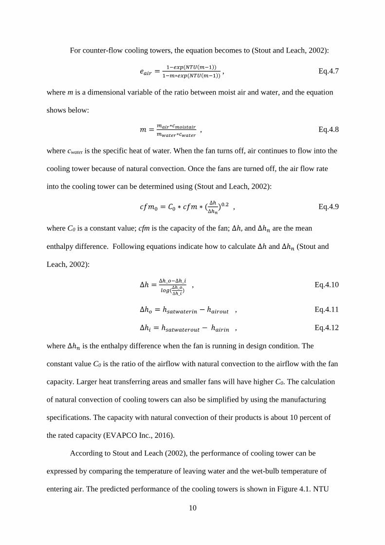
entering air. The predicted performance of the cooling towers is shown in Figure 4.1. NTU
11
can be determined once the c and n values, the design conditions, and the flow rate of water
and air were known. Then, the effectiveness of air can be calculated using Equation. 4.6 or
Equation 4.7 depends on the type of cooling tower. Based on Equation 3.1 and Equation. 4.4,
if the enthalpy of entering air and the temperature of entering water are known, the enthalpy
of leaving air can be determined. The temperature of leaving water can be determined using
Equation. 4.13:
𝑇𝑤𝑎𝑡𝑒𝑟𝑜𝑢𝑡 =𝑐𝑝𝑤𝑎𝑡𝑒𝑟∗𝑚𝑤𝑎𝑡𝑒𝑟𝑖𝑛∗𝑇𝑤𝑎𝑡𝑒𝑟𝑖𝑛−𝑚𝑎𝑖𝑟∗(ℎ𝑎𝑖𝑟𝑜𝑢𝑡−ℎ𝑎𝑖𝑟𝑖𝑛)
𝑐𝑝𝑤𝑎𝑡𝑒𝑟∗𝑚𝑤𝑎𝑡𝑒𝑟𝑜𝑢𝑡 Eq. 4.13
Figure 4.1 Performance Predictions (Stout and Leach, 2002)
According to Stout and Leach (2002), the NTU was found first via Equation 4.3 only
to lead directly to the effectiveness of air through Equation. 4.6 and Equation. 4.7. If the
effectiveness of air can be found without calculating NTU, the NTU will be no longer
needed. The idea is explained in Section. 9.1 of this thesis.

12
CHAPTER 5
EMPIRICAL MODEL
The performance of a cooling tower can be estimated via empirical curve fits. An
empirical model requires the wet-bulb temperature of entering air, range temperature, and
mass flow rate of air and water at design condition. The objective of the empirical model is to
estimate the approach temperature at different fan operating conditions.
The empirical model was built based on CoolTools correlation and YorkCalc
correlation that applied in EnergyPlus (EnergyPlus, 2014). These empirical models estimate
the approach temperature using a polynomial curve fit with the amount of coefficients and
either three or four independent variables. CoolTools is software released by Pacific Gas and
Electric Company (PG&E), and the objective is to develop, disseminate, and promote a tool
for design and operation of chilled water plants. CoolTools products are Internet-based,
public domain resources, and are targeted to building owners, design professionals, and
operators involved in both new construction and retrofits. Unfortunately, the CoolTools is no
longer available for users and was removed from the website of PG&E for an unknown
reason. YorkCalc model was developed by York International Corporation simulating the
performance of their produced chiller systems. Johnson Controls used $3.2 billion to acquire
York International Corporation in 2005, and the information of YorkCalc was no longer
shown on their website since that day.
Figure 5.1 shows the CoolTools correlation has 35 coefficients and requires four
independent variables (Benton, Bowman, Hydeman & Miller, 2002):

13
Figure 5.1 CoolTools Equations (EnergyPlus, 2014)
Figure 5.2 YorkCalc Equations (EnergyPlus, 2014)

14
Figure 5.2 shows the YorkCalc correlation has 27 terms with four independent
variables (York Co., 2002). The user needs to enter all coefficients to the equations to finish
simulation. The coefficients for both CoolTools and YorkCalc are shown below (EnergyPlus,
2014).
Figure 5.3 Coefficients of CoolTools and YorkCalc (EnergyPlus, 2014)
Both of CoolTools and YorkCalc models have their limitations and were shown in
Figure 5.4. YorkCalc is more flexible than CoolTools because YorkCalc can accept larger
range and approach temperatures. Since CoolTools and YorkCalc are developed based on
specific types of cooling towers and chiller systems, different coefficients and constraints
need to be determined to use on another system.

15
Figure 5.4 Limitations of CoolTools and YorkCalc (EnergyPlus, 2014)
16
CHAPTER 6
COOLING TOWER SPECIFICATIONS
Once the Effectiveness-NTU model and the empirical model were made using
MATLAB, a field test was prepared to validate both models. The cooling tower used in the
validation located behind AIME building at the University of Alabama. All the measuring
equipment were ordered at Onset Computer Corporation. Experimental protocols were
written and ready to apply to any other field tests. All collected data were analyzed and used
to verify the models.
Basic specifications and properties of the cooling tower were gathered from online
research. The cooling tower used in the experiment was made by Marley Cooling Tower
Corporation in 1999, and the series number is NC4222GS. Marley Co. was acquired by SPX
Cooling Co., and no longer makes these series of cooling towers. However, there is a current
model called NC8403 has similar dimensions and specifications with NC4222GS. A sketch
of the cooling tower is shown in Figure 6.1, and it is a dual-entering cooling tower that has
two cells and connected by the pipes of entering water. The vents of entering air located on
both sides of the cooling tower and the dimension of each vent is 11.5 feet by 7.5 feet. The
vents of leaving air are located on the top of the cooling towers with diameters of 7 feet.
Other dimensions and sketches of NC8403 can be found in the handbook in NC Steel
Cooling Tower Engineering Data on their website (SPX Cooling Technologies, Inc., 2011).
According to the classifications of cooling towers, the cooling tower used in the experiment
is wet, cross-flow and mechanical draught with fans.

17
Figure 6.1 Sketch of the HVAC Cooling Tower in UA
(SPX Cooling Technologies, Inc., 2011)
Each of these fans was operated by a 25 horsepower motor made by Marathon
Electric. The motors were designed with two speeds by serving cooling towers. The RPM of
the motors is 1755, and the nominal effectiveness is 87.5%. Since each fan has three speeds
includes natural convection with fans turned off, there are six running statuses of the cooling
tower.
The entering water comes from two chillers and flows into the cooling tower through
the pipes of entering water, and the leaving water flows out to a water basin. Two pumps
made by Goulds Pumps Inc. pump the leaving water from the basin to the chiller. The
capacity of both pumps is 1020 GPM, and the head pressure is 72 feet. Each pump is
operated by a 25 horsepower motor made by GE Motors. According to the operation
procedure, each pump and chiller switching their operation every 15 days, and rarely turn on
at the same time.
Figure 6.2 Pictures of the HVAC Cooling Tower in UA

18
CHAPTER 7
EXPERIMENT
7.1 Procedure and Devices
Figure 7.1 Design of Experiment
An experiment was designed to collect data, estimate and validate the
Effectiveness-NTU model and empirical model. A graph of the designed experiment is
shown in Figure 7.1. The measurements include the air temperature and relative humidity, the
velocity of air, the pump pressure, and the power of the motors.
The Facilities Department of the University provided the temperature of entering and
leaving water, the flow rate of makeup water and the running statuses of fans and pumps. The
sensors and data loggers were installed as shown in Figure 7.1. All the data was collected
using RX3002 and UX90 data loggers made by Onset Computer Co. The RX3002 data

19
logger was powered by a 6W solar panel shown in Figure 7.2 (a), and the data was uploaded
to the cloud through wireless.
(a) (b) (c)
Figure 7.2 Experimental Equipment
(a) Data Logger RX 3002 (b) Pressure Sensor T-ASH-G2-500 (c) Hood for S-THB-M008
Air temperature and humidity were measured using S-THB-M008 at both air inlet and
outlet. The sensors record dry-bulb temperature and relative humidity of the air. Wet-bulb
temperature can be calculated using Equation. 3.1. Pump pressure was collected using T-
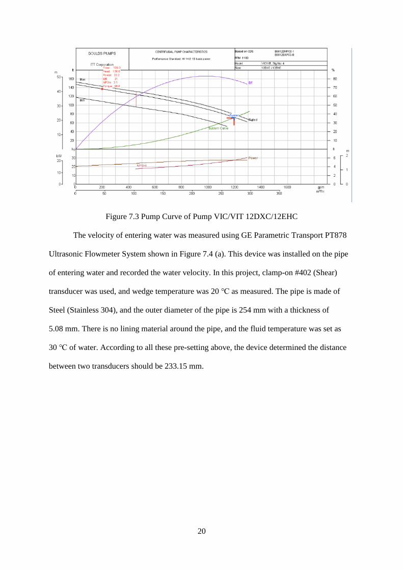
ASH-G2-500, which is shown in Figure 7.2 (b). The pump curve can be found by looking for
the series number of the pumps in Eprism released by Gouldspump Inc. (Gouldspump Inc.,
2016). The flow rate of leaving water can be found using the pump curve. Figure 7.3 shows
the pump curve of VIC/VIT pumps with a motor of 25 horsepower and 1770 RPM. In Figure
7.2 (c), a hood was assembled over the sensor on the top of the cooling tower to avoid solar
radiation.
20
Figure 7.3 Pump Curve of Pump VIC/VIT 12DXC/12EHC
The velocity of entering water was measured using GE Parametric Transport PT878
Ultrasonic Flowmeter System shown in Figure 7.4 (a). This device was installed on the pipe
of entering water and recorded the water velocity. In this project, clamp-on #402 (Shear)
transducer was used, and wedge temperature was 20 ℃ as measured. The pipe is made of
Steel (Stainless 304), and the outer diameter of the pipe is 254 mm with a thickness of
5.08 mm. There is no lining material around the pipe, and the fluid temperature was set as
30 ℃ of water. According to all these pre-setting above, the device determined the distance
between two transducers should be 233.15 mm.

21
(a) (b)
Figure 7.4 Experimental Equipment 2
(a) GE Parametric Transport PT878 Ultrasonic Flowmeter
(b) T-WNB-3D-480 transducer and SCT-0750 sensors
Fan and pump power were measured using T-WNB-3D-480 transducer and SCT-0750
sensors shown in Figure 7.4 (b). The current sensed by transducers generates a proportional
series of pulses, and the count of pulses was recorded by data loggers. The power of the
motor can be determined using the equation from the user manual of the device. According to
the user manual (Continental Control System, 2016), the equations applied in the
experimental cooling tower is:
𝑃𝑜𝑤𝑒𝑟 = 𝑊𝐻𝑝𝑃 ∗ 3600 ∗ 𝑃𝑢𝑙𝑠𝑒 𝐹𝑟𝑒𝑞𝑢𝑒𝑛𝑐𝑒 Eq. 6.1
where WHpP equals 5.7708, and the pulse frequency equals measured counts divided by 300.
Air velocity was measured using T-DCI-F99-L-P at the vent of entering air. The unit
of the velocity is foot per minute. The volumetric flow rate can be determined by multiplying
the velocity by the area of the vents. The mass flow rate can be calculated by multiplying
volumetric flow rate by air density.

22
7.2 Experiment Protocol
The frequency of recording data was every 5 minutes. Handheld devices are
recommended to use to double-check the measurements read by sensors. Figure 7.5 shows
handheld devices of air velocity and pump pressure.
Figure 7.5 Handheld Devices
Because the area of the air vent is large, the air speed varies at different locations on
the vent. At least ten measurements should be done at each location of the vent using
handheld air velocity device to reduce the variance of measurements. The locations are
shown in Figure 7.7 (a). Comparing the average velocity with the center point yields the ratio
between air velocity at a center point and average velocity. The ratio of this cooling tower is
1.24 when the fan was running at high speed. Additionally, measurements of air velocity at
low speed and stopped running statuses were needed to be captured and recorded. The
airspeed sensor should locate in the center of the vent, and the average airspeed can be
calculated by multiply the ratio by the measurements.
There are smart connections and analog connections between sensors and loggers.
Smart connections can easily plug into the data logger, but analog connections require
additional power startup. The frequency of power startup must be defined before the analog-
connecting sensors can start reading or recording data.

23
GE Parametric Transport PT878 Ultrasonic Flow Meter System is complicated to use
and readout. The material, diameter, flow direction and thickness of the pipe must be known.
The flow meter can only transfer data through infrared radiation, which is an outdated
technology and lost connections all the time. The flow meter is not waterproof, and the
battery can only last 2 hours. Therefore, the flow meter must be used indoors and connected
to a charger.
One must be extremely careful when installing power sensors and transducers. The
high voltage in the electrical cabinet can kill people. Make sure the switch was turned off,
and assure safety for oneself and any assistants.
(a) (b)
Figure 7.7 (a) Points of Measurements (b) Analog Connection

24
CHAPTER 8
MEASURED DATA ANALYSIS
The purpose of data analysis is testing if the collected data is accurate enough to be
used to validate the models. The verification processes include collecting data, calculating
variables, and validating results. The period of the data collection is from August 25 to
September 1, 2016, and the frequency is every 5 minutes.
Data was collected from three sources include data logger, ultrasonic flow meter, and
the Facilities Department of the University of Alabama. The data logger records the relative
humidity and the dry-bulb temperature of entering and leaving air, the pump pressure, the
velocity of entering air and the power of fan and pump motors. The facility provides the
running status of pumps and fans, the flow rate of makeup water, and the temperature of
entering and leaving water. The ultrasonic flow meter records the flow rate and velocity of
entering water. However, the result cannot apply in the analysis because of numerous errors
due to the operation failure. Therefore, the mass flow rate of entering water was calculated by
the sum of the mass flow rate of leaving water and make-up water.
The wet-bulb temperature was calculated using relative humidity and dry-bulb
temperature based on Equation. 3.1. Velocity and flow rate of the leaving water were
determined using pump pressure and the pump curve in Figure 7.3. Figure 7.7 (a) shows the
measured areas of vent, which is used to calculate velocity and the flow rate of air. Enthalpy
of the entering and leaving air was computed based on psychrometric equations in Chapter. 3.
The temperature of leaving water can be found using Equations. 4.13.
25
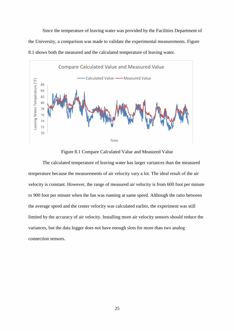
Since the temperature of leaving water was provided by the Facilities Department of
the University, a comparison was made to validate the experimental measurements. Figure
8.1 shows both the measured and the calculated temperature of leaving water.
Figure 8.1 Compare Calculated Value and Measured Value
The calculated temperature of leaving water has larger variances than the measured
temperature because the measurements of air velocity vary a lot. The ideal result of the air
velocity is constant. However, the range of measured air velocity is from 600 foot per minute
to 900 foot per minute when the fan was running at same speed. Although the ratio between
the average speed and the center velocity was calculated earlier, the experiment was still
limited by the accuracy of air velocity. Installing more air velocity sensors should reduce the
variances, but the data logger does not have enough slots for more than two analog
connection sensors.
70
72
74
76
78
80
82
84
86
Leav
ing
Wat
er T
emp
erat
ure
(℉
)
Time
Compare Calculated Value and Measured Value
Calculated Value Measured Value

26
Table 8.1 shows the statistical result of regression analysis between the two sets of
data.
Table 8.1 Regression Analyses
Regression Statistics
Multiple R 0.86 R Square 0.74 Adjusted R Square 0.74 Standard Error 1.34
Observations 2017
Table 8.2 Data Analysis
Calculated Value
Measured Value
Mean 76.82
Mean 77.81
Standard Error 0.058
Standard Error 0.04231
Median 76.80
Median 77.90
Mode #N/A
Mode 79.1
Standard Deviation 2.62
Standard Deviation 1.90
Sample Variance 6.89
Sample Variance 3.61
Kurtosis -0.54
Kurtosis -0.41
Skewness 0.185
Skewness 0.091
Range 13.341
Range 9
Minimum 70.940
Minimum 73.7
Maximum 84.281
Maximum 82.7
Sum 154953.12
Sum 156962.4
Count 2017
Count 2017
Another statistical result shows root mean square error (RMSE) of these two data is
1.71; The coefficient of variation mean square error (CV-RMSE) is 2.2%; The normalized
mean bias error (NMBE) is 3.8%; The normalized root mean square error (NRMSE) is
12.8%; The R-squared value between measured data and calculated data equals to 0.7402. As
a result, the experimental data is accurate enough to use in both Effectiveness-NTU and
empirical models because the CV-RMSE and NMBE of the calculated data meet the
requirements from ASHRAE Guideline 14. The frequency of measured data was 5 minutes,

27
and it was modified to 1 hour to verify the accuracy with ASHRAE’s requirements. The
recommended value of ASHRAE Guideline 14 is shown in Figure 8.2 (ASHRAE, 2014).
Figure 8.2 Recommended Value for Baseline Model by ASHRAE (2014)

28
CHAPTER 9
MODEL VALIDATION
Experimental data was used to validate both Effectiveness-NTU and empirical
models. The outputs of Effectiveness-NTU model are NTU and the effectiveness of air; the
output of the empirical model is approach temperature. Both models were validated by
comparing experimental measurements and the outputs from the models. Since the mass flow
rate of air is difficult to measure in most circumstances, all models were modified to use the
mass flow rate of air as an output, and a comparison was made between both models. The
wet-bulb temperature was calculated using experimental measurements from HOBO data
logger and the leaving water temperature was provided by Facilities Department. Since the
sources of data are different, the approach temperature of the cooling tower shows negative
values sometimes. The range of the negative values is from 0℉ to -1℉, but the approach
temperature should be greater than 0. Therefore, modifications of the data were made on
negative approach temperature. Once the approach temperature shows less than 0, it was
modified to 0. Then the leaving temperature of water at that time was changed equal to the
wet-bulb temperature of the entering air.
9.0 Psychrometric Equations
Measuring the temperature and relative humidity of leaving air is limited by safety,
accessibility, and accuracy. Instead of measuring the temperature of leaving air, a model was
developed using psychrometric equations to calculate the temperature of leaving air. A
validation process was done between the measured dry-bulb temperature and the calculated
dry-bulb temperature of leaving air. Since the relative humidity of leaving air is almost 100%
29
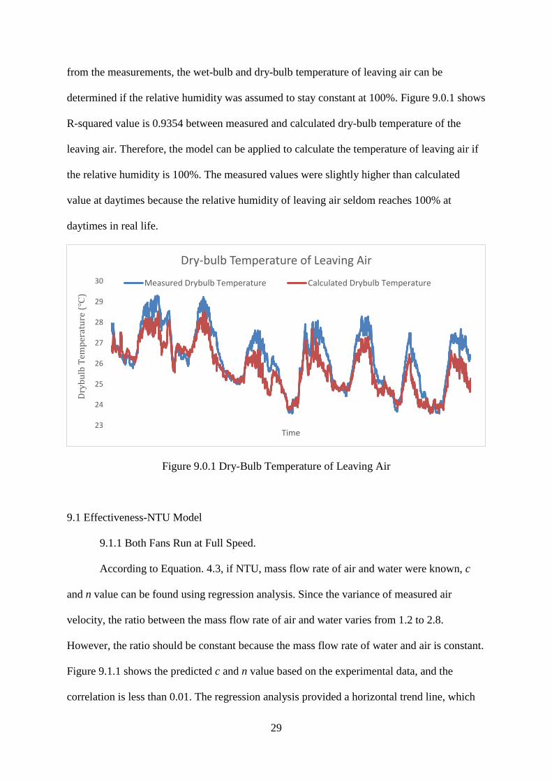
from the measurements, the wet-bulb and dry-bulb temperature of leaving air can be
determined if the relative humidity was assumed to stay constant at 100%. Figure 9.0.1 shows
R-squared value is 0.9354 between measured and calculated dry-bulb temperature of the
leaving air. Therefore, the model can be applied to calculate the temperature of leaving air if
the relative humidity is 100%. The measured values were slightly higher than calculated
value at daytimes because the relative humidity of leaving air seldom reaches 100% at
daytimes in real life.
Figure 9.0.1 Dry-Bulb Temperature of Leaving Air
9.1 Effectiveness-NTU Model
9.1.1 Both Fans Run at Full Speed.
According to Equation. 4.3, if NTU, mass flow rate of air and water were known, c
and n value can be found using regression analysis. Since the variance of measured air
velocity, the ratio between the mass flow rate of air and water varies from 1.2 to 2.8.
However, the ratio should be constant because the mass flow rate of water and air is constant.
Figure 9.1.1 shows the predicted c and n value based on the experimental data, and the
correlation is less than 0.01. The regression analysis provided a horizontal trend line, which
23
24
25
26
27
28
29
30
Dry
bu
lb T
emp
erat
ure
(℃
)
Time
Dry-bulb Temperature of Leaving Air
Measured Drybulb Temperature Calculated Drybulb Temperature

30
cannot be used for prediction. Figure 9.1.2 shows the prediction based on c=0.5038 and
n=0.365, and the result shows the NTU values are almost constant. Therefore, the
Equation. 4.3 is not recommended to use in this case because of lacking experimental
measurements. Since the mass flow rate of air and water were constant during the
experiment, one way to improve the estimation is taking more measurements from various
ratios between the mass flow rate of air and water. Another way to improve the accuracy is
minimum the variance of the measured airspeed.
Figure 9.1.1 Prediction of c&n value
Figure 9.1.2 Compare Measured NTU and Predicted NTU
Since the trend line in Figure 9.1.1 cannot use to predict c and n value, other
equations regarding the effectiveness of air were found. The effectiveness of air and approach
y = 0.5038x0.365
R² = 0.0007
0
1
2
3
4
5
6
7
8
1 1.2 1.4 1.6 1.8 2 2.2 2.4 2.6 2.8 3
NTU
ma/mw
C and N
0
2
4
6
NTU
Time
NTU ValidationCalculated NTU Measured NTU

31
temperature can both be determined using experimental measurements. Figure 9.1.3 indicates
the correlation between the approach temperature and the effectiveness of air.
Figure 9.1.3 Compare Approach Temperatures and Effectiveness of Air 1
Figure 9.1.3 shows the R-squared value of the red trend line is 0.4703 between
approach temperature and effectiveness of air. As the approach temperature decreases, the
effectiveness of air rises. Therefore, a power equation was found at the condition of both fans
running at full speeds:
𝑒𝑎𝑖𝑟 = 0.4354 ∗ 𝐴𝑝𝑝𝑟𝑜𝑎𝑐ℎ−0.267 Eq. 9.1
In Figure 9.1.3, a power trend line of Equation. 9.1 is shown in red; an exponential
trend line is shown in green; another linear trend line is shown in yellow. The linear equation
is not applied in this case because the linear equation generates negative effectiveness of air
once the approach temperature exceeds 8 ℉. The exponential equation is not applied because
the effectiveness of air should equal to 1 instead of 0.6 when the approach temperature is
0 ℉. However, the exponential equation shows a reasonable trend when approach
temperature is greater than 8 ℉. The power trend line indicates the effectiveness of air nearly
constant when the approach temperature is greater than 8 ℉, but the effectiveness of air
y = 0.4354x-0.267
R² = 0.4703
0
0.1
0.2
0.3
0.4
0.5
0.6
0.7
0.8
0.9
1
0 2 4 6 8 10 12 14
Effe
ctiv
enes
s o
f A
ir
Approach Temperature(℉)
Approach and Effectiveness of Air

32
should go to zero as approach temperature increases. A better prediction requires more data
in winter when the approach temperature is larger, and the effectiveness of air is smaller.
The R-squared value between the effectiveness of air that calculated by Equation. 4.4
and Equation. 9.1 is 0.8434. The data implemented in this test was taken from August 25 to
August 31, 2016, with a frequency of 5 minutes, and both of fans ran at high speed during
this period. Another set of data with different fan running status was imported due to another
running status in next section.
9.1.2 One Run in Full, One Stops.
This group of data was imported to represent another fan running status. The
measurements were taken from June 21 to July 25, 2016, at a frequency of 5 minutes with
one of the fans ran at full speed, and another stopped. The data lacks the temperature and the
relative humidity of leaving air, so calculations based on Section. 9.0 were applied to
determine the temperature of the leaving air at first. Then, the correlation between approach
temperature and effectiveness of air were calculated and plotted.
Figure 9.1.4 Compare Approach Temperatures and Effectiveness of Air 2
y = 0.5061x-0.193
R²= 0.7589
00.10.20.30.40.50.60.70.80.9
1
0 2 4 6 8 10 12 14
Effe
ctiv
enes
s o
f A
ir
Approach Temperature(℉)
Approach and Effectiveness of Air
33
Figure 9.1.4 shows the R-squared value is 0.7589 between approach temperature and
effectiveness of air. A power equation was found when one fan runs at full speed, and another
stops:
𝑒𝑎𝑖𝑟 = 0.5061 ∗ 𝐴𝑝𝑝𝑟𝑜𝑎𝑐ℎ−0.193 Eq. 9.2
The R-squared value between the effectiveness of air that calculated by Equation.4.4
and Equation. 9.2 is 0.8109. The coefficients in the Equations 9.2 are slightly different from
Equation 9.1 because the equations were predicted based on the different running statuses of
fans. Therefore, a combination of both groups of data was made in next section.
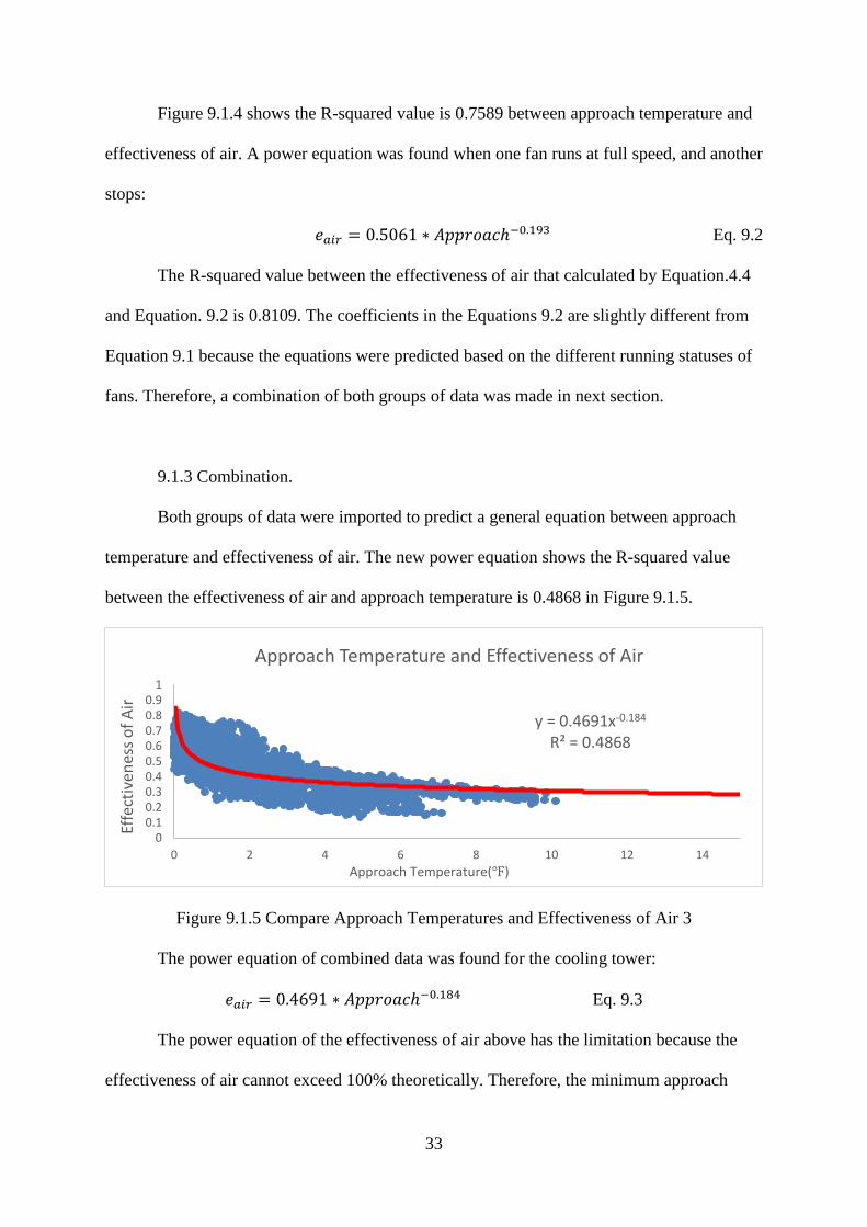
9.1.3 Combination.
Both groups of data were imported to predict a general equation between approach
temperature and effectiveness of air. The new power equation shows the R-squared value
between the effectiveness of air and approach temperature is 0.4868 in Figure 9.1.5.
Figure 9.1.5 Compare Approach Temperatures and Effectiveness of Air 3
The power equation of combined data was found for the cooling tower:
𝑒𝑎𝑖𝑟 = 0.4691 ∗ 𝐴𝑝𝑝𝑟𝑜𝑎𝑐ℎ−0.184 Eq. 9.3
The power equation of the effectiveness of air above has the limitation because the
effectiveness of air cannot exceed 100% theoretically. Therefore, the minimum approach
y = 0.4691x-0.184
R² = 0.4868
00.10.20.30.40.50.60.70.80.9
1
0 2 4 6 8 10 12 14
Effe
ctiv
enes
s o
f A
ir
Approach Temperature(℉)
Approach Temperature and Effectiveness of Air

34
temperature can apply to this equation is 0.018 ℉. Since the effectiveness of air increase
while the approach temperature raises, the approach temperature less than 0.018 ℉ gives the
effectiveness of air equals to 100% in this case.
Additionally, the relationship between approach temperature and relative humidity of
entering air was found. The correlation of R-squared value was as weak as 0.13, but Figure
9.1.6 shows the approach temperature increases while the relative humidity rises. It means
dryer entering air can lower the approach temperature and provide better performance to
cooling towers.
Figure 9.1.6 Relative Humidity and Approach Temperature
9.1.4 Validation.
Data from May 24 to June 1, 2016, was imported to validate Equation 9.3. Since this
data does not have measured temperature and humidity of leaving air either, a calculation
according to Section. 9.0 was applied to determine the dry-bulb temperature of leaving air
and assumed the relative humidity is 100%. The R-squared value of effectiveness of air
calculated using Equation.4.4 and Equation. 9.2 is 0.8025. Figure 9.1.7 shows the result of
comparisons. Since the correlation is strong enough, Equation 9.3 is ready to use in future
estimations.
-5
0
5
10
15
0
20
40
60
80
100
Ap
pro
ach
Tem
per
atu
re (
℉)
Rel
ativ
e H
um
idit
y (%
)
Time
Relative Humidity and Approach TemperatureRH_in Approach(F)

35
Figure 9.1.7 Effectiveness of Air Validation
9.2 Empirical Model
According to the equation on Figure 5.2, approach temperature can be determined
using empirical model. The input variables include the temperature of entering and leaving
water, the temperature and the relative humidity of entering air, the YorkCalc coefficients,
and the flow rate of air and water at design condition. The flow rate of air at design condition
was set as 168 kg/s, which is the amount of mass flow rate of two fans running at full speed.
The flow rate of water at design condition is 128 kg/s that is the sum of two pumps operating
at capacity. The YorkCalc model was selected instead of CoolTools model because the
YorkCalc model shows in Figure 5.3 has a larger range of limitation. The data was applied
from August 25 to August 31, 2016, with a frequency of 5 minutes, and both of fans ran at
high speed during this period.
Figure 9.2.1 shows a comparison between measured and calculated approach
temperature using the equation in Figure 5.2. The R-squared value between two approach
temperatures is 0.28. The R-squared value between the effectiveness of air from
Effectiveness-NTU model is 0.8025, so the results from YorkCalc model shows less
correlation than Effectiveness-NTU model. The reason is the YorkCalc model was designed
0.2
0.3
0.4
0.5
0.6
0.7
0.8
0.9e_
air
Time
Effectiveness of Air Validation
Calculated e_air Measured e_air
36
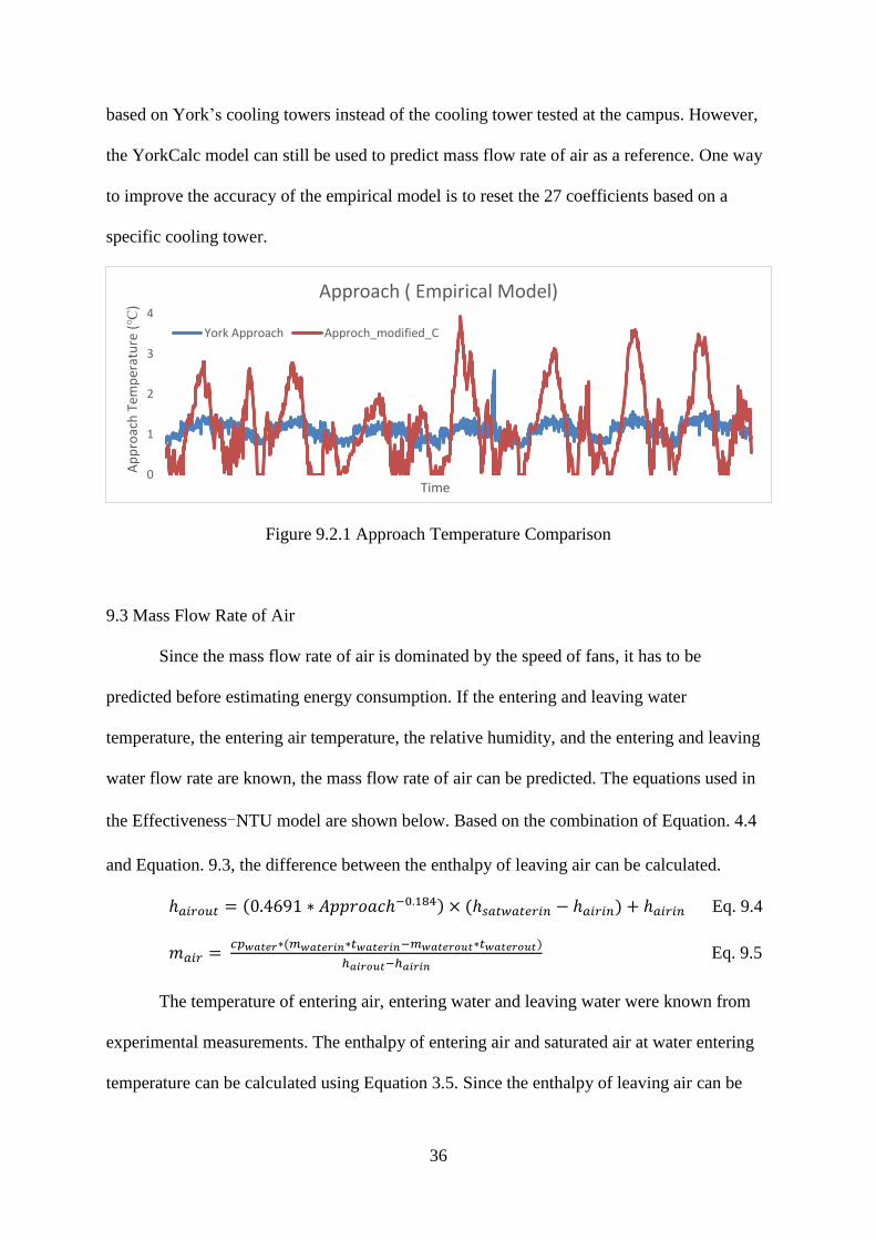
based on York’s cooling towers instead of the cooling tower tested at the campus. However,
the YorkCalc model can still be used to predict mass flow rate of air as a reference. One way
to improve the accuracy of the empirical model is to reset the 27 coefficients based on a
specific cooling tower.
Figure 9.2.1 Approach Temperature Comparison
9.3 Mass Flow Rate of Air
Since the mass flow rate of air is dominated by the speed of fans, it has to be
predicted before estimating energy consumption. If the entering and leaving water
temperature, the entering air temperature, the relative humidity, and the entering and leaving
water flow rate are known, the mass flow rate of air can be predicted. The equations used in
the Effectiveness-NTU model are shown below. Based on the combination of Equation. 4.4
and Equation. 9.3, the difference between the enthalpy of leaving air can be calculated.
ℎ𝑎𝑖𝑟𝑜𝑢𝑡 = (0.4691 ∗ 𝐴𝑝𝑝𝑟𝑜𝑎𝑐ℎ−0.184) × (ℎ𝑠𝑎𝑡𝑤𝑎𝑡𝑒𝑟𝑖𝑛 − ℎ𝑎𝑖𝑟𝑖𝑛) + ℎ𝑎𝑖𝑟𝑖𝑛 Eq. 9.4
𝑚𝑎𝑖𝑟 = 𝑐𝑝𝑤𝑎𝑡𝑒𝑟∗(𝑚𝑤𝑎𝑡𝑒𝑟𝑖𝑛∗𝑡𝑤𝑎𝑡𝑒𝑟𝑖𝑛−𝑚𝑤𝑎𝑡𝑒𝑟𝑜𝑢𝑡∗𝑡𝑤𝑎𝑡𝑒𝑟𝑜𝑢𝑡)
ℎ𝑎𝑖𝑟𝑜𝑢𝑡−ℎ𝑎𝑖𝑟𝑖𝑛 Eq. 9.5
The temperature of entering air, entering water and leaving water were known from
experimental measurements. The enthalpy of entering air and saturated air at water entering
temperature can be calculated using Equation 3.5. Since the enthalpy of leaving air can be
0
1
2
3
4
Ap
pro
ach
Tem
per
atu
re (
℃)
Time
Approach ( Empirical Model)
York Approach Approch_modified_C
37
calculated using Equation. 9.4, the mass flow rate of air based on energy balance can be
determined using Equation. 9.5 shows above.
The equation used in Empirical-YorkCalc model is according to the theory of
Empirical-YorkCalc model based on Figure 5.2:
𝑚𝑎𝑖𝑟 = 𝑓𝑟𝑎𝑖𝑟
𝑚𝑎𝑖𝑟𝑑𝑒𝑠𝑖𝑔𝑛 Eq. 9.6
where 𝑓𝑟𝑎𝑖𝑟 is the airflow rate ratio and 𝑚𝑎𝑖𝑟𝑑𝑒𝑠𝑖𝑔𝑛 is the mass flow rate of the air at design
condition.
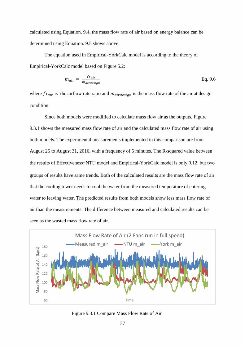
Since both models were modified to calculate mass flow air as the outputs, Figure
9.3.1 shows the measured mass flow rate of air and the calculated mass flow rate of air using
both models. The experimental measurements implemented in this comparison are from
August 25 to August 31, 2016, with a frequency of 5 minutes. The R-squared value between
the results of Effectiveness-NTU model and Empirical-YorkCalc model is only 0.12, but two
groups of results have same trends. Both of the calculated results are the mass flow rate of air
that the cooling tower needs to cool the water from the measured temperature of entering
water to leaving water. The predicted results from both models show less mass flow rate of
air than the measurements. The difference between measured and calculated results can be
seen as the wasted mass flow rate of air.
Figure 9.3.1 Compare Mass Flow Rate of Air
60
80
100
120
140
160
180
Mas
s Fl
ow
Rat
e o
f A
ir (
kg/s
)
Time
Mass Flow Rate of Air (2 Fans run in full speed)
Measured m_air NTU m_air York m_air

38
CHAPTER 10
ANNUAL PREDICTION
10.1 Range Prediction
Range temperature represents the temperature between the entering and leaving water.
From the previous measurements, the correlation was found between the dry-bulb
temperature of the entering air and the range temperature of the cooling tower. The
correlation shows when the dry-bulb temperature of air drops, the range of water temperature
drops as well. Since all measurements from the experiment were taken at summertime, the
range of dry-bulb temperatures only varies from 70 ℉ to 85 ℉. The dry-bulb temperature
was divided into groups by every 5 ℉, and the average range temperature was found for each
group. Table 10.1.1 shows the result of the dry-bulb temperature of the entering air and the
average range temperature.
Table 10.1.1 Average Range Temperature from Measurement
Variations of Dry-Bulb Temperature of Entering Air (℉) Average Range (℉)
70 75 5.14
75 80 5.75
80 85 6.48
Once the average range temperature at different variations of entering air temperature
was found, the relationship can be determined. Figure 10.1.1 shows a power equation
between the lower bound of entering air dry-bulb temperature and the average range
temperature. The R-squared value is 0.9968, and the equation of the trend line is:
𝑇𝑟𝑎𝑛𝑔𝑒 = 0.0033 ∗ 𝑇𝑙𝑜𝑤𝑒𝑟𝑏𝑜𝑢𝑛𝑑 1.7324 Eq. 10.1.1
where 𝑇𝑟𝑎𝑛𝑔𝑒 is the range temperature and 𝑇𝑙𝑜𝑤𝑒𝑟𝑏𝑜𝑢𝑛𝑑 is the lower bound of entering air
dry-bulb temperature.

39
Figure 10.1.1 Correlation of Average Range Temperature
In Figure 10.1.1, a linear trend line is shown in yellow, and the range temperature
shows less than zero once the lower bound of entering air dry-bulb temperature below 30 ℉.
Since cooling towers can operate in cold temperature as low as 5 ℉ (SPX Inc., 2016) and the
range temperature should greater than 0, the linear trend line cannot apply in this case. From
the Equation. 10.1.1, the other average range temperature of the cooling tower can be
estimated based on different variations of the dry-bulb temperature of entering air, and the
result is shown in Table 10.1.2.
y = 0.0033x1.7324
R² = 0.9982
0
2
4
6
8
10
0 20 40 60 80 100
Ave
rage
Ran
ge (
℉)
Lower Bound of Dry-Bulb Temperature of Entering Air (℉)
Range Prediction

40
Table 10.1.2 Prediction of Range Temperature
Variations of Dry-Bulb Temperature of Entering Air (℉)
Average Range (℉)
5 10 0.05
10 15 0.18
15 20 0.36
20 25 0.59
25 30 0.87
30 35 1.20
35 40 1.56
40 45 1.97
45 50 2.41
50 55 2.90
55 60 3.42
60 65 3.97
65 70 4.56
70 75 5.19
75 80 5.85
80 85 6.54
85 90 7.26
90 95 8.02
95 100 8.80
100 105 9.62
10.2 Predict Leaving Temperature
The relationship between the temperature of the entering air and leaving water is
shown in the Figure 10.2.1. The experimental measurements indicate the temperature of
leaving water increases when the temperature of the entering air rises. The linear equation of
the trend line is:
𝑇𝑤𝑎𝑡𝑒𝑟𝑜𝑢𝑡 = 0.1763 ∗ 𝑇𝑎𝑖𝑟𝑖𝑛 + 63.619 Eq. 10.2.1
where 𝑇𝑤𝑎𝑡𝑒𝑟𝑜𝑢𝑡 is the temperature of leaving water and 𝑇𝑎𝑖𝑟𝑖𝑛 is the dry-bulb temperature of
entering air. The reason to use linear function is the minimum leaving water of a cooling
tower cannot be less than 55 ℉ (Johnson Control, 2015). A power trend line is shown in
green and it exceeds the limitation of low-temperature condition.

41
Figure 10.2.1 Dry-bulb Temperature of Entering Air and Temperature of Leaving Water
10.3 Annual Weather Data
The weather data in Tuscaloosa, AL area in 2014 were provided by the weather
station located on the roof of Hardaway Hall, and the measurements include both dry-bulb
temperature and relative humidity. The frequency of the data is one hour, so there is a total of
8760 sets of data for a year. Wet-bulb temperature can be calculated using Equation. 3.1
based on the psychrometric equations.
10.4 Prediction
10.4.1 Effectiveness-NTU Model.
Since the annual wet-bulb temperature of the entering air can be calculated, the range
of water temperature and the temperature of leaving water can be determined using
Equation. 10.1.1 and Equation. 10.2.1. The range of water temperature and the temperature of
leaving water were calculated and plotted in Figure 10.4.1.
y = 0.1763x + 63.619
0
10
20
30
40
50
60
70
80
90
0 10 20 30 40 50 60 70 80 90 100Tem
per
atu
re o
f Le
avin
g W
ater
(℉
)
Temperature of Air at Entering(℉)
Dry-bulb Temperature of Entering Air and Temperature of Leaving Water

42
Figure 10.4.1 Temperature of Leaving Water and Range Temperature
Since the temperature of leaving water and range temperature were known, the
temperature of entering water of the cooling tower equals to:
𝑇𝑤𝑎𝑡𝑒𝑟𝑖𝑛 = 𝑇𝑤𝑎𝑡𝑒𝑟𝑜𝑢𝑡 + 𝑅𝑎𝑛𝑔𝑒 Eq. 10.4.1
where 𝑇𝑤𝑎𝑡𝑒𝑟𝑖𝑛 is the temperature of entering water, and 𝑇𝑤𝑎𝑡𝑒𝑟𝑜𝑢𝑡 is the temperature of
leaving water. The approach temperature can be calculated using:
𝐴𝑝𝑝𝑟𝑜𝑎𝑐ℎ = 𝑇𝑤𝑎𝑡𝑒𝑟𝑜𝑢𝑡 − 𝑇𝑤𝑏𝑖𝑛 Eq. 10.4.2
where 𝑇𝑤𝑏𝑖𝑛 is the wet-bulb temperature of entering air. The effectiveness of air can be
determined using Equation. 9.3; the enthalpy of leaving air can be calculated using
Equation. 9.4. Since the enthalpy of leaving air of the cooling tower were found, the mass
airflow rate can be calculated using following equation:
𝑚𝑎𝑖𝑟 = 𝐶𝑝𝑤𝑎𝑡𝑒𝑟∗(𝑚𝑤𝑎𝑡𝑒𝑟𝑖𝑛∗𝑇𝑤𝑎𝑡𝑒𝑟𝑖𝑛−𝑚𝑤𝑎𝑡𝑒𝑟𝑜𝑢𝑡∗𝑇𝑤𝑎𝑡𝑒𝑟𝑜𝑢𝑡)
ℎ𝑎𝑖𝑟𝑜𝑢𝑡−ℎ𝑎𝑖𝑟𝑖𝑛 Eq. 10.4.3
where Cpwater is the constant specific heat of water, and it equals to 4.178kJ/kg; mwaterout is the
constant mass flow rate of leaving water, which equals to 64.35kg/s. The constant makeup
water flow rate equals to 0.03 kg/s, and the constant mass flow rate of entering water equals
to 64.38 kg/s. The temperature of entering and leaving water was calculated earlier using
Equation. 10.2.1 and Equation. 10.4.1. The enthalpy of entering air can be determined using
0
2
4
6
8
10
40
50
60
70
80
90
Ran
ge T
emp
erat
ure
(℉)
Tem
per
atu
re o
f Le
avin
g W
ater
(℉
)Temperature of Leaving Water and Range Temperature (℉)
T_water_out_modified range
43
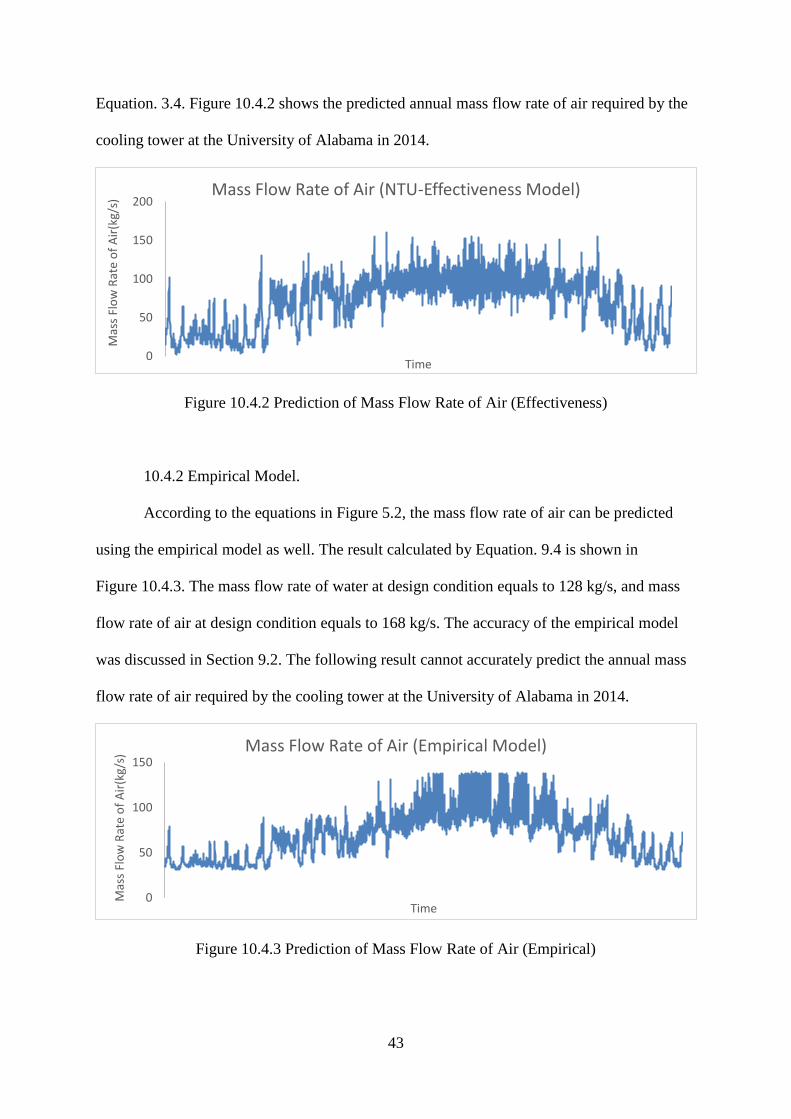
Equation. 3.4. Figure 10.4.2 shows the predicted annual mass flow rate of air required by the
cooling tower at the University of Alabama in 2014.
Figure 10.4.2 Prediction of Mass Flow Rate of Air (Effectiveness)
10.4.2 Empirical Model.
According to the equations in Figure 5.2, the mass flow rate of air can be predicted
using the empirical model as well. The result calculated by Equation. 9.4 is shown in
Figure 10.4.3. The mass flow rate of water at design condition equals to 128 kg/s, and mass
flow rate of air at design condition equals to 168 kg/s. The accuracy of the empirical model
was discussed in Section 9.2. The following result cannot accurately predict the annual mass
flow rate of air required by the cooling tower at the University of Alabama in 2014.
Figure 10.4.3 Prediction of Mass Flow Rate of Air (Empirical)
0
50
100
150
200
Mas
s Fl
ow
Rat
e o
f A
ir(k
g/s)
Time
Mass Flow Rate of Air (NTU-Effectiveness Model)
0
50
100
150
Mas
s Fl
ow
Rat
e o
f A
ir(k
g/s)
Time
Mass Flow Rate of Air (Empirical Model)

44
10.5 Different Fan Conditions
The cooling tower used in this project has two of 2-speeds fans. Each of the fans can
operate in three statuses: high, low, and stop. Air velocity of each fan was measured during
the experiment, and the mass flow rate was calculated. Since the power of the fans at capacity
was recorded, power of the fans in different conditions can be found using mass flow rate of
air based on the Affinity Law (Whitesides, 2012):
(𝑄1
𝑄2)3 =
𝑃1
𝑃2 Eq. 10.5.1
where Q is the mass flow rate, and P is the power. The power of the fans was calculated for
each status, and the result is shown in Table 10.5.1. Since two fans equipped on the cooling
tower, there are six combinations of running statuses, and each of them has a different mass
flow rate of air and power. Table 10.5.2 shows the mass flow rate of air and power of each
running status.
Table 10.5.1 Single Fan Conditions
Fan Condition Mass Air Flow Rate (kg/s) Fan Power (kW)
High 80.00 18.00
Low 32.00 1.15
Stop 8.00 0.00
Table 10.5.2 Dual Fans Conditions
Fan 1-Fan 2 Mass Air Flow Rate (kg/s) Fan Power (kW)
High-High 160.00 36.00
High-Low 112.00 19.15
High-Stop 88.00 18.00
Low-Low 64.00 2.30
Low-Stop 40.00 1.15
Stop-Stop 16.00 0.00
Because the annual mass flow rate and dual fans running statuses were both predicted,
an annual prediction of the fan running statuses can be found in Figure 10.5.1 based on the
predicted mass flow rate of air. For example, if the predicted mass flow rate of air is between
160 kg/s and 112 kg/s, the cooling tower requires both fans run at high speed. If the predicted

45
mass flow rate of air is less than 16 kg/s, the cooling tower can use natural convection by
shutting down both fans.
Figure 10.5.1 Annual Fan Running Status
According to Affinity Law, the annual energy consumption of current 2-speeds fans is
55,265 kWh, and the annual energy of variable speed fans is 33,205 kWh. The energy
consumption will be 302,328 kWh if both of the fans run at high speed for the whole year. A
comparison is shown in Table 10.5.3. As a result, variable speeds fans can save nearly
20,000 kWh for a year. Compared to single speed fans, 2-speeds fans can save close to
100,000 kWh for a year.
Table 10.5.3 Compare Energy Consumption
Single-Speed Fans 2-Speeds Fans Variable Speeds Fans
Annual Energy Consumption (kWh)
203,742 106,514 87,502
As a comparison, the energy consumption of a similar cooling tower was found. The
data was generated by the software called UPDATE (SPX Cooling Technologies, Inc., 2016).
The specifications and energy consumption were listed in Figure 10.5.2 (SPX Cooling
Technologies, Inc., 2016).
0
20
40
60
80
100
120
140
160
Mas
s fl
ow
rat
e o
f ai
r (k
g/s)
Air Mass Flow Rate in Different Fan Conditions
High-High High-Low High-Stop Low-Low Low-Stop Stop-Stop

46
Figure 10.5.2 Energy Consumption of NC8402 (SPX Cooling Technologies, Inc., 2016)
The differences in energy consumption between single-speed fans and 2-speeds fans
are huge, and 2-speeds fans with 6 stages of capacity controls are good enough for most of
the cooling towers. Although the result shows the variable speeds fans can save nearly 20,000
kWh, a benchmarking needs to be done to find out if it is worth to switch from 2-speeds fans
to variable speed fans because variable-speed motors cost much more.

47
CHAPTER 11
CONCLUSION
The goal of this project is to investigate and compare the performance of cooling
towers using Effectiveness-NTU model and empirical model. The processes to achieve the
goal include: Developed Effectiveness-NTU and empirical models of the cooling tower, and
predicted the performance of the design and off-design conditions; Stated experimental
protocols and gathered data on the HVAC cooling tower on the campus of the University of
Alabama; Used collected data to validate the models; Compared results from models with
real measurements and found the limitation of each model; Applied known annual weather
data to estimate the performance and energy consumption of the cooling tower;
Recommended the approach for the best energy and heat performance.
All data and specifications were gathered and measured from the experiment on
campus. In fact, the mass flow rate of air and the temperature of leaving air are not always
possible to gather from different cooling towers, especially industry cooling towers.
Therefore, both models were designed to predict mass flow rate of air, and the temperature of
leaving air by applying the temperature and the relative humidity of entering air. Fan status
and energy consumption of cooling tower were predicted according to the mass flow rate of
air. Total annual energy consumption of single-speed, 2-speeds, and variable-speed cooling
towers were calculated.
As a result, the NTU equation in the Effectiveness-NTU model is not applied in this
case, and another model regards effectiveness of air was built and tested. The effectiveness
model was built based on a regression analysis of the experimental data. The R-squared value
was 0.8 between the measured data and the predicted data. More data from lower outside air

48
temperature is needed to improve the accuracy. The empirical model built based on YorkCalc
correlations provided approach temperature, and the result has larger variances compared to
measured data. Another set of correlations relates to the testing cooling tower needs to be
developed.
A dual-speed cooling tower can save 50% of the energy, and a variable-speed cooling
tower can save 60% compared to a single-speed cooling tower. This result only applies to the
cooling tower used in the experiment, and the results of other cooling towers may vary. The
recommendation on choosing fan speeds for a cooling tower should consider: Cooling
tower’s life; Cost of energy; Cost of equipment; Payback period.
Further testing is required to validate the accuracy of the models because there was a
limited control over the running status of fans. More experimental data needs to be collected
in wintertime with the lower temperature of entering air. Validations on other cooling towers
are essential in the future. Additionally, the accuracy of the empirical model can be improved
by resetting all coefficients.
49
REFERENCES
ASHRAE, (2014). ASHRAE Guideline 14-2014, Standard & Guidelines Available from:
https://www.ashrae.org/standards-research--technology/standards--guidelines/titles-
purposes-and-scopes#Gdl14
Benton, D.J., Bowman, C.F., Hydeman, M.Miller, P. (2002). An Improved Cooling Tower
Algorithm for the CoolTools Simulation Model. ASHRAE Transactions, Vol. 108,
Part 1, pp. 760-768
Continental Control System LLC. , (2016). WattNode Pulse Installation and Operation
Manual, Power and Energy Equations, Rev V17b
EnergyPlus Documentation, (2014). Cooling Towers and Evaporative Fluid Coolers,
Simulation Models- Encyclopedic Reference, Retrieved from:
https://www.energyplus.net/sites/default/files/docs/site_v8.3.0/EngineeringReference/
13-EncyclopaedicRefs/index.html
EVAPCO ICT Cooling Towers, (2016) EVAPCO Inc. P.O.Box 1300, Westminster,
Maryland 21158, 10M/9682/FB, page 12
F. P. Incropera, D.P. DeWitt, T.L. Bergaman, and A.S. Lavine, (2007). Fundamentals of Heat
and Mass Transfer, 6th Ed.
Gouldspump Inc., (2016). Eprism Software, Pump Curve, Available from:
https://eprism.gouldspumps.com/prism/
Johnson Control, Inc., (2015). Model YK Centrifugal Liquid Chiller Style H, 250 through
600 tons (897 through 2110 kW) Available from: http://www.johnsoncontrols.com/-
/media/jci/be/united-states/hvac-
equipment/chillers/files/be_yk_engineeringguide_h.pdf?la=en
L.Lu, W.Cai, (2002). A Universal Engineering Model for Cooling Towers, International
Refrigeration, and Air Conditioning Conference. Paper 625
Malcolm J. MacPherson, (1993). Psychrometric: the study of moisture in air, 14-1 to 14-28,
Subsurface Ventilation and Environmental Engineer, Springer Netherlands
Malcolm R. Stout Jr., James W. Leach, (2002). Cooling Tower Fan Control for Energy
Efficiency. Energy Engineering Vol.99, No.1
Randall W. Whitesides, (2012). Basic Pump Parameters and the Affinity Laws, PDHonline
Course M125, Retrieved from:
http://www.pdhonline.com/courses/m125/m125content.pdf

50
SPX Cooling Technologies, Inc., (2011). Engineering Data, Marley NC Steel Cooling Tower,
Pg 14-16. Retrieved from: http://spxcooling.com/library/detail/marley-nc-class-
cooling-tower-engineering-data1/
SPX Cooling Technologies, Inc., (2016). Cold Weather Operation of Cooling Towers,
Associated with Water Cooled Chiller Systems. Thermal Science, Marley Available
from: http://www.spxcooling.com/TR-015.pdf
SPX Cooling Technologies, Inc., (2016). Marley, VFD-Motor Package Insight, Retrieved
from: http://spxcooling.com/library/detail/marley-insight-vfd-motor-package
SPX Cooling Technologies, Inc., (2016). UPDATE Software, Design Condition, and Version
5.1.4 Available from: http://qtcapps.ct.spx.com/update/Inputs.aspx
Viska Mulyandasari, (2011). KLM Technology Group, Cooling tower selection, and sizing,
Engineering design guidelines. Rev: 01 Retrieved from:
http://www.klmtechgroup.com/PDF/EDG/ENGINEERING%20DESIGN%20GUIDE
LINES%20-%20Cooling%20Towers%20-%20Rev01.pdf
York International Corporation, (2002). YORKcalc Software, Chiller-Plant Energy-
Estimating Program, Form 160.00-SG2 (0502)