Control Engineering Practice 100 (2020) 104442

Contents lists available at ScienceDirect

Control Engineering Practice

journal homepage: www.elsevier.com/locate/conengprac

Energy optimal control of an over-actuated hybrid feed drive undervariable-frequency disturbances — with application to machiningMolong Duan ∗, Keval S. Ramani, Chinedum E. OkwudireDepartment of Mechanical Engineering, University of Michigan, 2350 Hayward, Ann Arbor, MI 48109, United States of America

A R T I C L E I N F O

Keywords:Energy efficiencyControl allocationGain schedulingMachiningFeed drive

A B S T R A C T

Machine tool feed drives are often subject to variable-frequency disturbance (cutting) forces due to varyingspindle speeds or cutting tools. A proxy-based control allocation method has been proposed for energyoptimal control of over-actuated systems (i.e., systems with more actuators than the number of outputs tobe controlled). It has been applied to an over-actuated hybrid feed drive, consisting of a linear motor drivecoupled to a screw drive, and its effectiveness has been demonstrated under fixed-frequency disturbanceforces. This paper discusses the fundamental limit of the fixed-frequency approach and extends the proxy-basedcontrol allocation method to account for variable-frequency disturbance forces via a linear parameter-varyingformulation. The controller gains are optimized using linear matrix inequality and scheduled as a functionof disturbance frequency. Significant improvements in energy efficiency are demonstrated in simulations andexperiments using the proposed gain-scheduling approach compared to the existing fixed-frequency approach.

1. Introduction

There is a growing appreciation of the need to reduce the energyconsumption of machine tools without unduly sacrificing quality andproductivity (Duflou et al., 2012; Helu et al., 2012). Feed drives areresponsible for coordinated motion delivery in machine tools. Hence,they play a critical role in the quality and productivity of machiningprocesses (Altintas et al., 2011); but they also account for a significantportion of machine tool energy consumption (Vijayaraghavan & Dorn-feld, 2010), especially when they are driven by linear motors. Amongthe research on energy consumption reduction of machine tools, energyefficiency enhancement of feed drive is an important topic. Many ofthe energy efficiency enhancement approaches focus on optimized tra-jectories, controllers, or workpiece locations. For example, Mori et al.(2011) reduced energy consumption, in part, by synchronizing spindleand feed drive motions. Denkena, Hesse, and Gümmer (2009) proposedan energy optimal design of jerk-decoupled feed axes. Mohammad,Uchiyama, and Sano (2015) and Farrage and Uchiyama (2018) reducedthe energy consumption of the feed drive by enhancing the settlingperformance through sliding mode controllers. Wang et al. (2018)proposed a cloud-based energy-efficient approach in the context ofrobotic manufacturing. Sato, Shirase, and Hayashi (2018) investigatedthe optimization of workpiece locations for energy efficiency. Theseoptimization techniques reduce energy consumption but are usuallylimited by the hardware. Therefore, redundant actuation is increasinglyused to further enhance energy efficiency. Halevi, Carpanzano, andMontalbano (2014) proposed minimum energy control of a redundantly

∗ Corresponding author.E-mail address: molong@umich.edu (M. Duan).

actuated feed drive. Du, Plummer, and Johnston (2017) developedan energy-efficient control method for an electrical-hydraulic hybridmotion control system. Okwudire and Rodgers (2013) proposed a hy-brid feed drive (HFD), consisting of a linear motor drive (LMD) and atraction screw drive (SD). The HFD is shown in cutting tests to achievesimilar positioning precision as an equivalent LMD with up to 80%higher efficiency (Kale, Dancholvi, & Okwudire, 2014).

The HFD is an over-actuated system, i.e., it has more actuators thanthe number of outputs to be controlled. Over-actuation is often adoptedin feed drive systems, and the synergistic cooperation among the redun-dant actuators is the core control focus (Altintas & Sencer, 2010; Haleviet al., 2014; Schmidt et al., 2017). In the HFD, the primary controlobjective is to determine an optimal combination of LMD and SDefforts to achieve a desired level of positioning precision using the leastcontrol energy from both actuators. Existing control allocation meth-ods (i.e., methods for optimally distributing control efforts) are eithercomputationally expensive or involve approximations that deterioratepositioning precision when applied to over-actuated systems like theHFD (Duan & Okwudire, 2018). Recently, Duan and Okwudire have de-veloped a new approach called proxy-based control allocation (PBCA)for dual-input (Duan & Okwudire, 2018) and multi-input (Duan &Okwudire, 2017) over-actuated systems, and have analyzed its relation-ship to linear quadratic control (Duan & Okwudire, 2019). The PBCAmethod converts the control allocation problem for a redundant systemto a standard regulation problem of a derived control energy proxy,thus enabling computationally inexpensive control allocation without

https://doi.org/10.1016/j.conengprac.2020.104442Received 19 September 2019; Received in revised form 24 April 2020; Accepted 28 April 2020Available online 15 May 20200967-0661/© 2020 Elsevier Ltd. All rights reserved.

M. Duan, K.S. Ramani and C.E. Okwudire Control Engineering Practice 100 (2020) 104442

deteriorating positioning performance. The effectiveness of PBCA wasdemonstrated on the HFD, where up to 95% improvement in efficiencywas achieved without sacrificing positioning performance. However, amajor drawback of the work presented in Duan and Okwudire (2018)is that, in employing the PBCA, the dominant disturbance frequencieswere assumed to be fixed. However, in machining processes, distur-bance frequencies change regularly, e.g., due to changing spindle speedor cutting tools with differing number of flutes. Therefore, the primarycontributions of this paper are in:

(1) Analytically demonstrating the fundamental limitations of thefixed-frequency PBCA approach by converting the fixed-frequency PBCA design problem into a tracking control problemof a non-minimum phase system.

(2) Proposing a variable-frequency PBCA approach where the pa-rameters of the PBCA are varied (scheduled) as a function ofdisturbance frequencies, allowing the allocator to change itsbehavior considering the process information.

The proposed variable-frequency PBCA is compared to the fixed-frequency PBCA (Duan & Okwudire, 2018) in simulations and ma-chining experiments, and large improvements in energy efficiency aredemonstrated. The rest of this paper is organized as follows. Section 2gives an overview of the HFD and the PBCA method. Section 3 an-alytically demonstrates the fundamental limit of the fixed-frequencyPBCA method and formulates the proposed variable-frequency PBCAapproach. Section 4 presents the simulation and experimental results,followed by the conclusions and future work in Section 5.

2. Overview of HFD and proxy-based control allocation

2.1. Hybrid feed drive (HFD)

Fig. 1(a) shows the schematic of an HFD prototype whose designis detailed in Okwudire and Rodgers (2013). It consists of an LMDdirectly connected to the moving table, and a traction SD which can beconnected to or disconnected from the table using a (dis)engagementmechanism and twist-roller friction drives. The LMD alone drives thetable during rapid traverse motions (while the SD is disengaged fromthe table). However, during machining, the LMD and SD both actuatethe table in parallel (i.e., they act in hybrid mode) to deliver similarpositioning precision as the LMD at much higher efficiency (Kale et al.,2014).

During the hybrid mode, the HFD can be modeled as a standard two-mass system (see Fig. 1(b)). In the figure, 𝑚1 and 𝑚2 are the (equivalent)masses of the rotating and translating components of the HFD, whilek and c represent the stiffness and viscous damping coefficient ofthe connecting mechanical components; 𝑥1, 𝑥2, and 𝑏1, 𝑏2 are the(equivalent) displacements and viscous damping coefficients at 𝑚1 and𝑚2, respectively; 𝑢1 and 𝑢2 are the (equivalent) control forces appliedby the rotary and linear motors, while 𝑑1 and 𝑑2 represent externaldisturbance forces (e.g., non-viscous friction and cutting forces) appliedto 𝑚1 and 𝑚2, respectively. Note that 𝑑1 = 0 can be assumed because thebearing friction at the rotary motor can be readily determined and com-pensated in feedforward; therefore, the only (dominant) disturbanceconsidered in this paper is the one acting on the table due to cuttingforces (denoted as 𝑑2 = 𝑑). Defining 𝑠 as the Laplace variable, thetransfer function matrix of the HFD, 𝐆, between the input forces (i.e.,𝐮 = {𝑢1, 𝑢2}T and 𝑑) and the output displacements (i.e., 𝐱 = {𝑥1, 𝑥2}T)is derived as (Duan & Okwudire, 2016)

𝑦 = 𝑥2 =[

𝐺1 𝐺2]

⏟⏞⏞⏞⏞⏞⏞⏟⏞⏞⏞⏞⏞⏞⏟𝐆

[

𝑢1 𝑢2 + 𝑑]T , (1)

where

𝐺1 =𝐺1𝑛𝐷

= 𝑐𝑠 + 𝑘𝐷

; 𝐺2 =𝐺2𝑛𝐷

=𝑚1𝑠2 +

(

𝑐 + 𝑏1)

𝑠 + 𝑘𝐷

;

𝐷 = 𝑎4𝑠4 + 𝑎3𝑠3 + 𝑎2𝑠2 + 𝑎1𝑠;

𝑎4 = 𝑚1𝑚2; 𝑎3 = 𝑏1𝑚2 + 𝑏2𝑚1 + 𝑐(

𝑚1 + 𝑚2)

;

𝑎2 = 𝑐(

𝑏1 + 𝑏2)

+ 𝑘(

𝑚1 + 𝑚2)

+ 𝑏1𝑏2; 𝑎1 =(

𝑏1 + 𝑏2)

𝑘.

(2)

2.2. Proxy-based control allocation method

The overall energy comsumption of feed drive systems is typicallyanalyzed considering the kinetic energy, the cutting energy, and theheat loss (Halevi et al., 2014; Kale et al., 2014). The kinetic energyand the cutting energy depend on the motion trajectory and cuttingconditions. The control allocation considered in this paper does notalter the motion trajectory nor the cutting conditions employed. There-fore, the heat loss is selected to be the energy efficiency metric to beminimized. The formulation of heat loss also agrees with the minimumenergy control (minimization of two norm of control actions) defined inthe control literature (Skogestad & Postlethwaite, 2007). For the HFD,this objective is defined as in (Duan & Okwudire, 2016)

𝐸ℎ𝑒𝑎𝑡 = ∫

(

𝑢1(𝑡)𝐾𝑚1

)2𝑑𝑡

⏟⏞⏞⏞⏞⏞⏞⏞⏞⏟⏞⏞⏞⏞⏞⏞⏞⏞⏟𝐸ℎ𝑒𝑎𝑡,1

+ ∫

(

𝑢2(𝑡)𝐾𝑚2

)2𝑑𝑡

⏟⏞⏞⏞⏞⏞⏞⏞⏞⏟⏞⏞⏞⏞⏞⏞⏞⏞⏟𝐸ℎ𝑒𝑎𝑡,2

. (3)

The parameter 𝐾𝑚𝑖 represents the (equivalent) motor constant of theith actuator (𝑖 = 1, 2); it is often reported in the specification sheetsof electric motors. The larger the motor constant, the more efficientthe motor (see Duan & Okwudire, 2018 for more details). To bestutilize the HFD in hybrid mode, optimal combination of 𝑢1 and 𝑢2 thatminimizes 𝐸ℎ𝑒𝑎𝑡 without sacrificing the positioning accuracy is desired.From Eq. (1), all possible control inputs (i.e., 𝐮) that yield the sametable position 𝑥2 under specific disturbance signal 𝑑 satisfy

𝑥2 = 𝐺1𝑢1 + 𝐺2(

𝑢2 + 𝑑)

⇒ 𝐺1𝛿𝑢1 + 𝐺2𝛿𝑢2 = 0, (4)

where 𝛿 represents the variational operator. Note that 𝛿𝑑 = 𝛿𝑥2 = 0because they are each fixed, though unknown, functions of time. Also,the most efficient control inputs must minimize 𝐸ℎ𝑒𝑎𝑡; i.e.,

𝛿

(

∫

(

(

𝑢1𝐾𝑚1

)2+(

𝑢2𝐾𝑚2

)2)

𝑑𝑡

)

= 0 ⇒𝑢1𝐾2𝑚1

𝛿𝑢1 +𝑢2𝐾2𝑚2

𝛿𝑢2 = 0. (5)

Combining Eqs. (4) and (5),𝑢1𝑢2

= 𝛽∗; 𝛽 ≜ 𝜅2𝐺1𝐺2, (6)

where 𝜅 = 𝐾𝑚1∕𝐾𝑚2. The implication of Eq. (6) is that to satisfy a given𝑥2 requirement at maximum efficiency, the control inputs are boundby an optimal transfer function relationship given by 𝛽∗. Note that ∗

represents the adjoint operation, which makes 𝛽∗ non-causal, meaningthat it cannot be evaluated in real time (Duan & Okwudire, 2018).To force 𝑢1 and 𝑢2 to obey the optimal relationship in real time, 𝛽∗is decomposed as

𝛽∗ =𝛽1𝛽2

=

⎛

⎜

⎜

⎜

⎜

⎜

⎝

𝑅22𝐺∗1𝑛 − 𝑅12𝐺∗

2𝑛𝜓

⏟⏞⏞⏞⏞⏞⏞⏞⏞⏞⏞⏟⏞⏞⏞⏞⏞⏞⏞⏞⏞⏞⏟≜𝛽1

⎞

⎟

⎟

⎟

⎟

⎟

⎠

⎛

⎜

⎜

⎜

⎜

⎜

⎝

𝑅11𝐺∗2𝑛 − 𝑅12𝐺∗

1𝑛𝜓

⏟⏞⏞⏞⏞⏞⏞⏞⏞⏞⏞⏟⏞⏞⏞⏞⏞⏞⏞⏞⏞⏞⏟≜𝛽2

⎞

⎟

⎟

⎟

⎟

⎟

⎠

−1

, (7)

and a proxy variable 𝑢𝐷 is defined as

𝑢𝐷 = 𝛽2𝑢1 − 𝛽1𝑢2, (8)

where 𝛽1 and 𝛽2 are causal transfer functions that can be readilydetermined using a process detailed in Duan and Okwudire (2018). Thisconcept of control alignment can also be used to estimate the energyperformance of an arbitrary controller, this alignment-based energyevaluation is detailed in Duan and Okwudire (2019).

2

M. Duan, K.S. Ramani and C.E. Okwudire Control Engineering Practice 100 (2020) 104442

Fig. 1. Schematic of (a) HFD prototype, and (b) two-mass model of HFD.

Fig. 2. Block diagram of the two-stage control framework using PBCA.

Notice that 𝑢𝐷 = 0 implies that 𝑢1∕𝑢2 = 𝛽∗. Moreover, as 𝑢𝐷 → 0,𝐸ℎ𝑒𝑎𝑡 monotonically approaches its minimum value (Duan & Okwudire,2018). In other words, the variable 𝑢𝐷 is a proxy for how far the systemis from its optimal efficiency. The farther from 0 the value of 𝑢𝐷 gets,the less efficient it becomes (Duan & Okwudire, 2018). This means thatenergy optimal control of the HFD can be achieved using a two-stageframework as shown in Fig. 2. In Stage 1, a controller 𝐂𝑝 is designedto determine 𝐮0 = {𝑢0,1, 𝑢0,2}T that forces 𝑥2 to track reference position,𝑥𝑟. A very straightforward way to design such a controller is to useonly one control input (i.e., assuming 𝑢0,1 = 0 or 𝑢0,2 = 0), and design asingle-input, single-output (SISO) controller to control 𝑥2 using the non-zero input. In Stage 2, a control allocator, 𝐂𝑎, is designed to distribute𝐮0 optimally to yield 𝐮. As shown in the expanded view of 𝐂𝑎, energyoptimal allocation is achieved by altering 𝑢𝐷 from its initial value of𝑢𝐷0 = 𝛽2𝑢0,1 − 𝛽1𝑢0,2 to 𝑢𝐷 → 0 (approaching optimal efficiency). Thiscan be achieved using a standard SISO controller, 𝐶𝑒. Notice from Fig. 2that 𝐮 is forced to satisfy the relationship

𝐮 = 𝐮0 +[

−𝐺2𝑛𝐷−1𝑑

𝐺1𝑛𝐷−1𝑑

]

𝑣 ⇒ 𝐆𝐮 = 𝐆𝐮0, (9)

where 𝑣 is the output of 𝐶𝑒, and 𝐷𝑑 (𝑠) is a user-specified replacementdenominator of original denominator 𝐷(𝑠) for allocator bandwidthcontrol (Duan & Okwudire, 2018). This structure in Eq. (9) ensuresthat 𝑥2 stays the same as was designed in Stage 1, even as 𝐮 isadjusted by 𝐶𝑒 to minimize 𝑢𝐷. In other words, Eq. (9) specifies adynamic null space structure for the over-actuated system. Moreover,this framework supports the saturation constraints on the allocatedcontrol effort through output–input constraints conversion. The mainidea is to convert the saturation limit to a state-dependent limit on thenulls space variable 𝑣. This constraints is especially helpful to alleviate

Fig. 3. Analogy to tracking controller design for the NMP system.

the undesirable slip in the friction drive shown in Fig. 1(a); more detailimplementation is discussed in Duan and Okwudire (2018).

3. Design of variable-frequency PBCA

3.1. Fundamental limit of time-invariant PBCA design

According to the analysis in Duan and Okwudire (2018), the twonorm of 𝑢𝐷 represents the deviation from energy optimality and thusshould be minimized. However, it is shown in this section that thereexists a fundamental limit to the regulation of 𝑢𝐷 to the desired valueof zero with a time-invariant PBCA controller. This means that 𝑢𝐷 = 0is unattainable, and an analytical lower bound is provided.

Consider the denominator 𝜓 , defined as a spectral decompositionrecommended in Duan and Okwudire (2018), i.e.,

𝜓∗𝜓 =[

𝐺∗2𝑛

−𝐺∗1𝑛

]T

𝐑[

𝐺2𝑛−𝐺1𝑛

]

. (10)

This definition ensures that the two-norm of 𝑢𝐷 strictly measures thedeviation from energy optimality. Then it can be derived, from Eqs. (7)and (10), that

𝛽1𝐺1𝑛 + 𝛽2𝐺2𝑛 =

[

𝐺∗2𝑛

−𝐺∗1𝑛

]T

𝐑[

𝐺2𝑛−𝐺1𝑛

]

𝜓= 𝜓∗. (11)

According to the definition of 𝑢𝐷 in Eq. (8) and the null space structurein Eq. (9), the control proxy before and after the allocation (𝑢𝐷0 and 𝑢𝐷)satisfy the relationship

𝑢𝐷 = 𝑢𝐷0 −𝛽1𝐺1𝑛 + 𝛽2𝐺2𝑛

𝐷𝑑𝑣 = 𝑢𝐷0 −

𝜓∗

𝐷𝑑𝑣. (12)

Accordingly, as shown in Fig. 3, the design of 𝐶𝑒 is identical to thedesign of a feedback tracking controller for an equivalent plant givenby 𝜓∗∕𝐷𝑑 . Note that 𝐷𝑑 is designed by the user and is guaranteed tobe a stable denominator, while 𝜓∗ contains non-minimum phase (NMP)zeros since 𝜓 is designed to have only minimum phase zeros (Duan &

3

M. Duan, K.S. Ramani and C.E. Okwudire Control Engineering Practice 100 (2020) 104442

Okwudire, 2018). Therefore, plant 𝜓∗∕𝐷𝑑 is a stable NMP system. Notethat the only possibility that 𝜓∗ does not contain NMP zeros is that𝜓∗𝜓 is a scalar, which corresponds to the trivial scenario where 𝐺1𝑛and 𝐺2𝑛 are both scalars such that inputs 𝑢1 and 𝑢2 cancel each otherprior to affecting the dynamics of the states. For an arbitrary lineartime-invariant design of 𝐶𝑒, the tracking performance of a stable NMPsystem has a fundamental limit. According to Chen, Qiu, and Toker(2000), the minimum tracking error of 𝑢𝐷 for a step input from 𝑢𝐷0 isgiven by

min𝐶𝑒 ∫

∞

0‖

‖

𝑢𝐷 (𝑡)‖‖

2 𝑑𝑡 =∑

𝑖

2Re(

𝑧𝑖)

|

|

𝑧𝑖||2

cos2 ∠(

𝜂𝑖, 𝑢𝐷0(

0+))

, (13)

where 𝑧𝑖 is the NMP zeros in plant 𝜓∗∕𝐷𝑑 and 𝜂𝑖 is the correspondingNMP zero direction vector. In the HFD setup, cos2 ∠ (𝜂𝑖, 𝑢𝐷0(0+)) = 1,since 𝑢𝐷0 and 𝑢𝐷 are scalar signals. According to Eqs. (7) and (11),

𝜓∗ =𝑚1𝑠2 − 𝑎𝜓1𝑠 + 𝑎𝜓0

𝐾𝑚1, (14)

where

𝑎𝜓1 =√

2𝑚1𝑘√

(1 + 𝛾) − 2𝑚1𝑘 +(

𝑐 + 𝑏1)2 + 𝛾𝑐2,

𝑎𝜓0 = 𝑘√

(1 + 𝛾),(15)

and 𝛾 = (𝐾𝑚,1∕𝐾𝑚,2)2 represents the energy efficiency ratio between thescrew drive and the linear motor drive. Therefore, the minimum valueof the expression in Eq. (13) is derived as

min𝐶𝑒 ∫

∞

0‖

‖

𝑢𝐷 (𝑡)‖‖

2 𝑑𝑡 = 2(

1𝑧1

+ 1𝑧2

)

=2𝑎𝜓1𝑎𝜓0

. (16)

This expression provides the fundamental limit on the time-invariant𝐶𝑒 design for the HFD in the time domain for a representative stepinput. In the frequency domain, since the analogous plant 𝜓∗∕𝐷𝑑is stable with NMP zeros, the fundamental limit can be interpretedusing the weighted Bode’s sensitivity integral formula (Skogestad &Postlethwaite, 2007), i.e.,

∫

∞

0ln|

|

|

|

𝑢𝐷 (𝑗𝜔)𝑢𝐷0 (𝑗𝜔)

|

|

|

|

⋅𝑤(

𝑧1, 𝑧2, 𝜔)

𝑑𝜔 = 0, (17)

where 𝑤(𝑧1, 𝑧2, 𝜔) is a weighting function given by

𝑤(

𝑧1, 𝑧2, 𝜔)

=∑

𝑖=1,2

Re(

𝑧𝑖)

Re(

𝑧𝑖)2 +

(

Im(

𝑧𝑖)

− 𝜔)2

=𝑎𝜓1

(

𝑎𝜓0 + 𝜔2)

𝜔4 −(

4𝑎2𝜓1 − 18𝑎𝜓0)

𝜔2 + 𝑎2𝜓0.

(18)

Note that w(𝑧1, 𝑧2, 𝜔) is positive for all 𝜔>0, and reaches itsmaximum when 𝜔≈|Im(𝑧1)| . This illustrates that the sensitivity of thewaterbed effect is especially high around the NMP zero frequencies.This fundamental limit indicates that 𝑢𝐷 = 0 is not achievable across awide range of disturbance frequencies due to the heightened waterbedeffect caused by the NMP zeros in plant 𝜓∗∕𝐷𝑑 , i.e., a time-invariant 𝐶𝑒designed to regulate 𝑢𝐷 over a wide frequency band would have verylimited effectiveness.

3.2. PBCA designs considering variable disturbance frequencies

Information from the reference trajectory and the cutting distur-bances can be used to facilitate more effective regulation 𝑢𝐷0 despitethe fundamental limit of the PBCA design derived in the precedingsection. Based on Fig. 3 and Eq. (12), the relationship between 𝑢𝐷 and𝑢𝐷0 can be expressed as

𝑢𝐷 = 11 + 𝐶𝑒

𝜓∗

𝐷𝑑

𝑢𝐷0. (19)

It has been analyzed in Section 3.1 that 𝑢𝐷 = 0 cannot be achieved overa wide range of disturbance frequencies with time-invariant 𝐶𝑒 designdue to the fundamental limitation of tracking accuracy in Eq. (16) and

waterbed effect specified in Eq. (17). However, 𝐶𝑒 can be designedto regulate 𝑢𝐷0 at its dominant frequencies to maximize the overallenergy efficiency (to reduce heat loss). As Fig. 2 indicates, 𝑢𝐷0 can betreated as the output of the reference 𝑥𝑟 and cutting force 𝑑. Due tolinear property, dominant frequency components in 𝑥𝑟 and 𝑑 are carriedinto 𝑢𝐷0. From these two sources, the disturbance force 𝑑 is dominantduring cutting since the motion is usually scheduled at constant or verysmooth velocity (i.e., the dynamic components in 𝑥𝑟 are less dominantthan those in 𝑑). The cutting force 𝑑 is usually periodic in the timedomain, resulting in its frequency components to be concentrated atzero frequency and discrete finite frequencies 𝑓𝑗 (𝑗 = 0, 1, 2,… , 𝑁 −1).Accordingly, 𝐶𝑒 can be designed, using the internal model principle(Duan & Okwudire, 2018), as

𝐶𝑒(𝑠) = 𝐾𝑒1

𝑠 + 𝜀

𝑁−1∏

𝑗=0

𝜔2𝑗

𝑠2 + 2𝜁𝑗𝜔𝑗𝑠 + 𝜔2𝑗

𝐻𝐿𝑃 (𝑠), (20)

where 𝐾𝑒 is the controller gain, and the next two terms provide highgains at zero frequency and at frequencies 𝜔𝑗 = 2𝜋𝑓𝑗 , respectively, if𝜀 and 𝜁𝑗 are selected to be very small numbers. Note that 𝜁𝑗 changesthe width of the peak around frequency 𝜔𝑗 , therefore it should bekept sufficiently large when there is uncertainty in 𝜔𝑗 . According tothe 3 dB rule in modal analysis (Inman, 2014), 𝜁𝑗 should be largerthan |𝛥𝜔𝑗 |∕(2𝜔𝑗 ) to guarantee robustness, where 𝛥𝜔𝑗 represent theuncertainty of disturbance frequency 𝜔𝑗 . Transfer function 𝐻𝐿𝑃 (𝑠) isa low-pass filter used to attenuate higher frequency content from 𝑑and ensure stability. Note from Eq. (19) that larger 𝐾𝑒 values lead tosmaller 𝑢𝐷, and the high resonant peak at 𝜔𝑗 guarantees large |𝐶𝑒(𝑗𝜔𝑗 )|,resulting in a very small spectrum component of 𝑢𝐷 at this frequency.The assumption implied in Eq. (20) is that the dominant frequencies of𝑑 are invariant (fixed). However, in most practical machining scenarios,the dominant frequencies can change with the change of spindle speedand cutting tools. Therefore, a design of 𝐶𝑒 considering the variablefrequency of the cutting disturbance is necessary.

For this purpose, the dominant frequency 𝜔𝑗 is relaxed to be a time-varying parameter, denoted as 𝜔𝑗 (𝑡). Here it is assumed that the timetrace of 𝜔𝑗 (𝑡) is known a priori (i.e., the change of frequency can happenat arbitrary time instant during the cutting operation and is knownto the controller). It is assumed that the rate of frequency variationis significantly slower compared to the feed drive control bandwidth.Moreover, the change in frequency can be continuous or discrete. Theseassumptions are usually satisfied in practical machining scenarios. Thisfrequency-based scheduling is also employed in screw drive controlwhere the resonant frequency is position-dependent (Hanifzadegan &Nagamune, 2013). With 𝜔𝑗 (𝑡), 𝐶𝑒 in Eq. (20) becomes a transfer func-tion with time-varying coefficients. It is realized using its controllablecanonical state–space realization such that the parameterized state–space matrices are guaranteed to be continuous with respect to varyingparameter 𝜔𝑗 (𝑡). Consider also the state–space representation of otherlinear time-invariant components in Fig. 3, the closed-loop system from𝑢𝐷0 to 𝑢𝐷 is represented by the following linear parameter varyingsystem:

�̇�𝑐 (𝑡) = 𝐀𝑐 (𝜔𝑗 (𝑡))𝐱𝑐 (𝑡) + 𝐁𝑐 (𝜔𝑗 (𝑡))𝑢𝐷0(𝑡)𝑢𝐷(𝑡) = 𝐂𝑐 (𝜔𝑗 (𝑡))𝐱𝑐 (𝑡) +𝐷𝑐 (𝜔𝑗 (𝑡))𝑢𝐷0(𝑡),

(21)

where 𝐱𝑐 (𝑡), 𝐀𝑐 (𝜔𝑗 (𝑡)), 𝐁𝑐 (𝜔𝑗 (𝑡)), 𝐂𝑐 (𝜔𝑗 (𝑡)), and 𝐷𝑐 (𝜔𝑗 (𝑡)) are the statevector, state matrix, input matrix, output matrix, and feedthrough term,respectively. This state–space realization uses observable canonicalform such that the physical meanings of the states at different 𝜔𝑗are consistent. Note that the changing parameter does not change thesystem order such that the size of 𝐀𝑐 , 𝐁𝑐 , 𝐂𝑐 , and 𝐷𝑐 are consistentfor different 𝜔𝑗 . The state matrix can be expressed using an affineparameter-dependent model (Symens, van Brussel, & Swevers, 2004)

𝐀𝑐 (𝜔𝑗 (𝑡)) = 𝐀0 +𝑀∑

𝑖=1𝜌𝑖(𝜔𝑗 (𝑡))𝐀𝑖, (22)

4

M. Duan, K.S. Ramani and C.E. Okwudire Control Engineering Practice 100 (2020) 104442

Fig. 4. Experiment setup: HFD mounted on a milling machine.

where 𝜌𝑖(𝜔𝑗 (𝑡)) ∈ [−1, 1], 𝐀0 and 𝐀𝑖 are constant matrices, and Mis the order (number of states) of the system. The system describedby Eqs. (21) and (22) is stable if there exists matrices 𝐏 > 0 and 𝐗𝑖(𝑖 = 1, 2,…,𝑀) such that the following linear matrix inequalities (LMIs)hold (Briat, 2014)

−𝐗𝑖 ±(

𝐀T𝑖 𝐏 + 𝐏𝐀𝑖

)

≤ 0; 𝐀T0𝐏 + 𝐏𝐀0 +

𝑀∑

𝑖=1𝐗𝑖 < 0, (23)

where ‘‘> 0’’ and ‘‘< 0’’ denote the positive and negative definiteness ofa matrix, respectively. Note that the satisfaction of Eq. (23) implies theexistence of a common quadratic Lyapunov function that guaranteesa stable system as controllers are switched rapidly to accommodatearbitrary variations in disturbance frequencies, 𝜔𝑗 (𝑡). This quadraticstability criterion is used to seek the maximum admissible values of𝐾𝑒 in Eq. (20). The procedure is detailed as follows. The maximal 𝐾𝑒values which guarantee the stability of the individual linear systemare firstly calculated. The corresponding affine parameter model inEq. (22) is then generated and verified for the common Lyapunovfunction condition in Eq. (23). If the common Lyapunov function isnot satisfied, the 𝐾𝑒(𝜔𝑗 ) values are iteratively reduced until Eq. (23)is satisfied. Note that the linear parameter varying system converges toa common stable linear invariant system when 𝐾𝑒 approaches 0, whichindicates the feasibility of 𝐾𝑒 values for the given LMI conditions inEq. (23).

4. Simulations and experiments

Simulations and machining experiments are conducted to demon-strate the effectiveness of the proposed variable-frequency (VF) PBCA,compared to the fixed-frequency (FF) PBCA and a baseline case (with-out control allocation). Fig. 4 shows the set-up used for the exper-iments, where the HFD is mounted on a FADAL vertical machiningcenter to enable milling at variable spindle speeds. The experimen-tally identified parameters of the HFD’s two-mass model are shownin Table 1. The parameters are acquired by fitting the experimentalfrequency response function to a two-mass model (Duan & Okwudire,2018). The (equivalent) motor constants for its rotary and linear motorsare 𝐾𝑚,1 = 380.8 N∕

√

W and 𝐾𝑚,2 = 21 N∕√

W, respectively. Therefore,𝜅2 = (𝐾𝑚,1∕𝐾𝑚,2)2 = 328.8, indicating two orders of magnitude differ-ence in the efficiencies of the two actuators. The cutting disturbanceis machining disturbance is assumed to be concentrated at a singlefrequency given by Jauregui et al. (2018)

𝑓0 =𝑛𝑟𝑝𝑚𝑛𝑓𝑙𝑢𝑡𝑒

60. (24)

where 𝑛𝑟𝑝𝑚 is the spindle speed in round per minute, and 𝑛𝑓𝑙𝑢𝑡𝑒 is thenumber of flutes in the milling tool. In simulation, additional biasedsinusoidal forces are generated from the linear motor to represent thecutting forces due to this frequency dominance.

Table 1Experimentally identified parameters of HFD’s two-mass model.𝑚1 [kg] 𝑚2 [kg] 𝑏1 [kg/s] 𝑏2 [kg/s] c [kg/s] k [N/μm]

616.2 46.3 44.8 83.3 5777.2 3.147

Fig. 5. Table’s reference speed (�̇�𝑟) and disturbance frequency (𝑓0) as functions of time.

4.1. Simulations

In simulations, the HFD’s table is commanded to travel at a constantspeed of 60 mm/min while disturbance 𝑑 = 𝐴(cos(2𝜋𝑓0t) −1) N isapplied to it, with 𝐴 = 100 N and 𝑓0 varying from 10 to 40 Hz in1 Hz increments, as shown in Fig. 5. The following controller cases areconsidered.

4.1.1. Baseline case (no control allocation)In Fig. 2, 𝐂𝑎 = 𝐈 (identity matrix) is assumed; 𝐂𝑝 is selected as

𝐮0 = 𝐂𝑝(

𝑥𝑟 − 𝑥2)

⏟⏞⏞⏟⏞⏞⏟𝑒2

=[

0 𝐾𝑝 +𝐾𝑖𝑠 + 𝐾𝑑 𝑠

𝑇𝑓 𝑠+1

]T𝑒2. (25)

The implication is that 𝐂𝑝 is a standard SISO PID controller appliedto the LMD; 𝐾𝑝, 𝐾𝑖, and 𝐾𝑑 are tuned to 7.46 × 106 N∕m, 4.07 ×106 N∕m∕s and 1.01 × 105 Ns∕m, respectively, and the time constantof the stabilizing low-pass filter is set at 𝑇𝑓 = 1.39 × 10−4 s.

4.1.2. Fixed-frequency (FF) allocation caseThe same 𝐂𝑝 from the baseline case is used. However, for 𝐶𝑒 =

𝐶𝑒,𝑓 𝑖𝑥𝑒𝑑 , a PBCA is designed for a fixed frequency 𝑓0 = 25 Hz (i.e., themedian of 10 to 40 Hz). Referring to Eq. (20) with 𝑁 = 1, 𝜀 =10−5 rad∕s and 𝜁 = 10−2 are selected to achieve very high gains at0 Hz and 25 Hz, respectively; 𝐻𝐿𝑃 is chosen such that the marginallystable denominator D (see Eq. (2)) is replaced with a stable 6th orderButterworth filter with a cut-off frequency of 𝑓0 + 10 Hz. Gain 𝐾𝑒 =501 N∕

√

W is then selected to ensure stability with a gain margin of 6dB, using standard controller tuning techniques.

4.1.3. Variable-frequency (VF) allocation caseThe same 𝐂𝑝 from the baseline case is used. For every discrete value

of 𝑓0, i.e., 10, 11, 12, . . . , 40 Hz, 𝐶𝑒, and 𝐻𝐿𝑃 are designed in a mannersimilar to that for FF allocation. However, to ensure that stability ismaintained as the gains are scheduled, for each value of 𝑓0, 𝐾𝑒 mustbe chosen such that Eq. (23) is satisfied. To do this, 𝐾𝑒 is selectedto achieve a 6-dB gain margin at each discrete 𝑓0 based on 𝐶𝑒,𝑓 𝑖𝑥𝑒𝑑 .Next Eq. (19) is converted to state–space form to determine 𝐀𝑐 , 𝐁𝑐 , 𝐂𝑐 ,and 𝐷𝑐 in (Eq. (21)) for all 𝑓0, based on the determined 𝐾𝑒 values.Matrices 𝐀0, 𝐀1,… ,𝐀𝑀 (with 𝑀 = 9) are then determined such that𝐀𝑐 for all 𝑓0 can be represented using the affine parameter-dependentmodel of Eq. (22). It is found that the condition in Eq. (23) is satisfied.This implies that the 𝐾𝑒 value with the 6-dB gain margin for each 𝑓0guarantee stability as the PBCA is scheduled as a function of 𝑓0. Theresulting values of 𝐾𝑒 as a function of 𝑓0 is shown in Fig. 6, wherethere are two drops at low- and high-frequency ranges. The drop in lowfrequency arises from the 1∕(𝑠 + 𝜀) term in Eq. (20), while the drop inhigh frequency arises from the physical limitation of the controllabilityfrom the non-collocated rotary motor.

5

M. Duan, K.S. Ramani and C.E. Okwudire Control Engineering Practice 100 (2020) 104442

Fig. 6. Gain 𝐾𝑒 as a function of 𝑓0 for variable-frequency allocator.

Fig. 7. Simulated positioning error and actuator heat loss using baseline,fixed-frequency, and variable-frequency allocator cases.

Table 2Simulated positioning error and actuator heat loss using baseline, fixed-frequency, andvariable-frequency allocator cases.

Baseline FF Allocator @ 25 Hz VF Allocator

𝑒2,rms [μm] 6.22 6.22 6.22𝐸ℎ𝑒𝑎𝑡,1[J] 0 16.10 28.17𝐸ℎ𝑒𝑎𝑡,2[J] 4505.63 330.18 36.85𝐸ℎ𝑒𝑎𝑡 [J] 4505.63 346.28 65.02

Table 3Cutting parameters.

Spindle speed (rpm) 300∕750∕1200

Tool 3/16’’ dia., 2-fluted, HSS end millWorkpiece 1018 cold finished mild steelFeed per tooth (mm/tooth) 0.03∕0.012∕0.0075Feed rate (mm/min) 18Lubrication None

Fig. 7 shows the simulated table positioning error 𝑒2 = 𝑥𝑟 − 𝑥2, aswell as the resultant 𝐸ℎ𝑒𝑎𝑡,1 and 𝐸ℎ𝑒𝑎𝑡,2 for the FF and VF allocators,compared with the baseline case (all using the �̇�𝑟 and 𝑓0 shown inFig. 5); Table 2 summarizes the results. Notice that the 6.22 μm RMSpositioning error is the same for all three cases. This is because thePBCA method guarantees that control allocation (i.e., Stage 2 of thetwo-stage process in Fig. 2) does not alter positioning performancedetermined in Stage 1. The FF allocator uses less the energy-efficientscrew drive and thus the for the 𝐸ℎ𝑒𝑎𝑡,1 for the FF allocator is lessthan VF allocator. This insufficient use of the screw drive leads toa significant increase in 𝐸ℎ𝑒𝑎𝑡,2. Therefore, although the FF allocatorgenerates 92% less heat compared to the baseline case, the proposedVF allocator generates 81% less heat compared to the FF allocator. The

proposed VF allocation approach is significantly more energy efficientcompared to the baseline and FF allocator.

4.2. Experiment

Cutting tests are carried out to verify the performance of the pro-posed VF allocator experimentally. Three 3 mm-long and 2 mm-deepslots are cut at different spindle speeds using cutting parameters re-ported in Table 3. Note that three discrete spindle speeds (i.e., 300,750 and 1200 rpm) are used in the experiments because the spindlespeed on the machine tool cannot be controlled to vary continuouslywith the motion of the HFD in a synchronized manner. A two-flutedend mill is used, so 300, 750 and 1200 rpm correspond to dominantcutting frequencies, 𝑓0, at 10, 25 and 40 Hz, respectively.

The three cases discussed in Section 4.1 are compared in the experi-ments. The only difference between the controllers used in simulationsand experiments is that 𝐂𝑝 is changed to

𝐮0 = 𝐂𝑝(

𝑥𝑟 − 𝑥2)

⏟⏞⏞⏟⏞⏞⏟𝑒2

=[

𝐾𝑝,1 +𝐾𝑖,1𝑠 +𝐾𝑑,1𝑠 𝐾𝑝,2 +𝐾𝑑,2𝑠

]T𝑒2 (26)

with gain values reported in Table 4. Essentially, in Eq. (26), 𝐂𝑝 ismade to also control the rotary motor (together with the linear motor)because, due to friction in the Roh’lix nut, the linear motor alone cannotback-drive the rotary motor. For the FF allocator case, 𝐶𝑒,𝑓 𝑖𝑥𝑒𝑑 designedbased on 25 Hz in Section 4.1.2 is used for cutting at the three spindlespeeds. Similarly, for the VF allocator, the 𝐶𝑒 designed for 10, 25 and40 Hz in Section 4.1.3 are respectively applied to cutting at 300, 750and 1200 rpm.

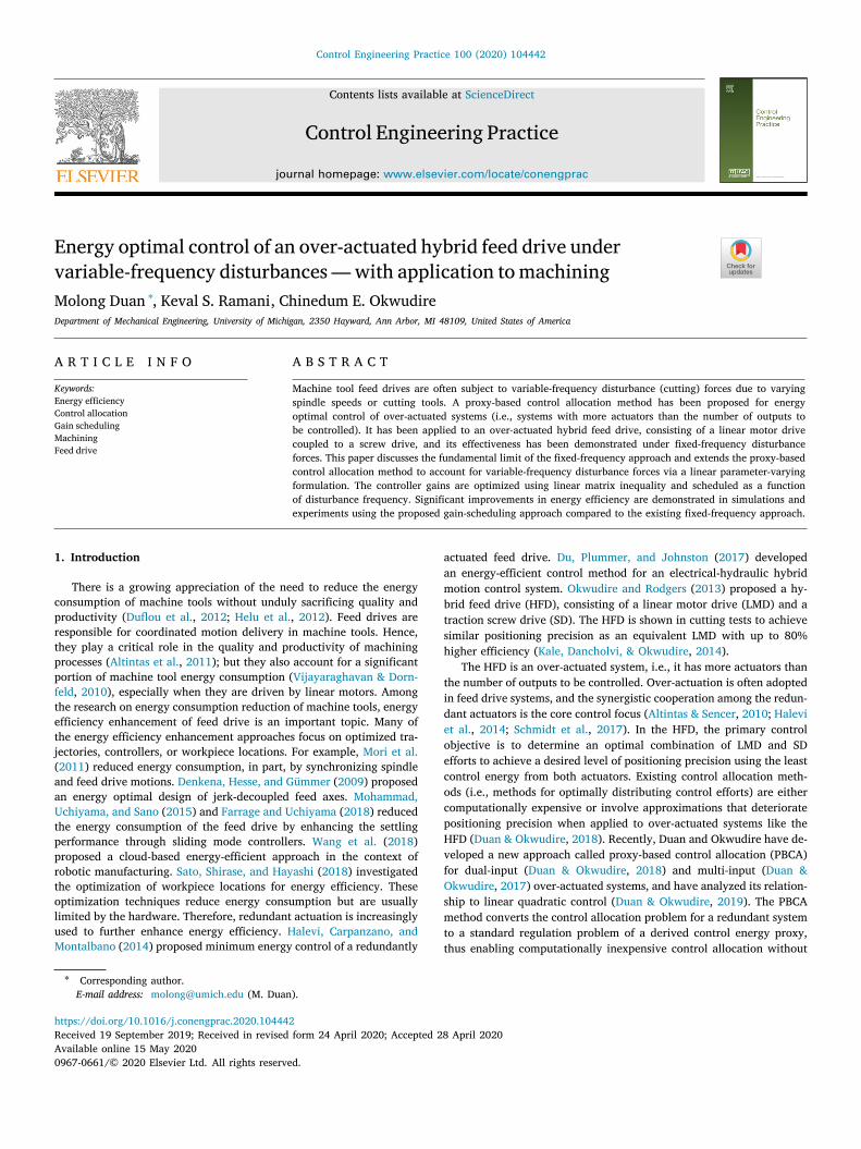
Fig. 8 shows 𝑒2 (measured from the linear encoder) as well as 𝐸ℎ𝑒𝑎𝑡,1and 𝐸ℎ𝑒𝑎𝑡,2 (calculated from the motor currents/forces using Eq. (3)) forthe baseline (BL), FF allocator and VF allocator cases; the results aresummarized in Table 5. Notice that, for each spindle speed, the RMSpositioning error is very similar among the three cases, again, due tothe properties of the PBCA method. The slight (≤0.5 μm) differencesamong the errors are due to modeling errors and slight variations inconditions that cannot be completely avoided in experiments. Notethat the positioning errors of the 300 rpm tests are a bit higher thanthose at 750 and 1200 rpm due to higher cutting forces at lowerspindle speeds. This higher cutting forces arise from the higher feedsper tooth, which increases with the mean cutting force at the feeddirection (Rubeo & Schmitz, 2016). At 1200 rpm, the proposed VFapproach generates 59% less heat than the baseline case, while theFF allocator generates 3% more heat than the baseline case becauseit is not tuned for dominant forces at 1200 rpm. The situation is worseat 300 rpm where the FF allocator generates almost 3 times moreheat compared to the baseline case, while the proposed VF allocatorgenerates 63% less heat compared to the baseline case. The resultsof the FF and VF allocators converge at 750 rpm, and generate both

Table 5Positioning error and actuator heat loss in cutting experiments using baseline,fixed-frequency, and variable-frequency allocator cases.

300 rpm 750 rpm 1200 rpm

BL FF VF BL FF VF BL FF VF

𝑒2,rms[μm] 2.7 2.4 2.8 1.8 2.0 2.0 2.4 2.5 2.0𝐸ℎ𝑒𝑎𝑡,1 [J] 4.8 5.3 5.2 4.6 5.6 5.6 10.9 11.2 8.8𝐸ℎ𝑒𝑎𝑡,2 [J] 27.2 121.4 6.7 14.7 6.1 6.1 32.9 34.0 9.2𝐸ℎ𝑒𝑎𝑡 [J] 32.0 126.7 11.9 19.4 11.8 11.8 43.8 45.2 18.0𝐸ℎ𝑒𝑎𝑡 reduction – −296% 63% – 39% 39% – −3% 59%

Table 4Values of 𝐂𝑝 controller gains in Eq. (26).

𝐾𝑝,1 [N ⋅ m−1] 𝐾𝑖,1 [N ⋅ m−1 ⋅ s−1] 𝐾𝑑,1 [N ⋅ m−1 ⋅ s] 𝐾𝑝,2 [N ⋅ m−1] 𝐾𝑑,2 [N ⋅ m−1 ⋅ s]

3.1 × 107 4.2 × 108 5.2 × 105 1.1 × 107 3.4 × 104

6

M. Duan, K.S. Ramani and C.E. Okwudire Control Engineering Practice 100 (2020) 104442

Fig. 8. Positioning error and actuator heat loss in cutting experiments using baseline, fixed- frequency, and variable-frequency allocator cases.

39% less heat compared to the baseline case. The comparison of heatlosses clearly illustrates the energy efficiency advantage of VF allocatorwithout sacrificing positioning accuracy.

Note that the simulation and experiment setting use different base-line controllers. The baseline control in the simulation uses only thelinear motor drive (𝑢2) for actuation, which illustrates the performancegain of the adoption of redundant actuation. In experiments, this pureuse of linear motor for actuation is not possible since it may me-chanically damage the reconfigurable friction drive. Since this baselinecontroller adopted already has a built-in level of control allocation,the energy performance gain is relatively smaller compared to thesimulation results. Also, it is clear that poor control alignment at thedisturbance frequency may introduce more energy consumption to thebaseline system. In this regard, the fixed frequency approach is notalways efficient, the accurate information of the disturbance frequencyis necessary for energy efficiency enhancements.

5. Conclusions and future work

The existing practice for designing proxy-based control allocator(PBCA) assumes that the disturbance force frequency is invariant(fixed). However, in machining applications, disturbance (i.e., cutting)force frequencies vary as spindle speed and cutting tools are changed. Itis analytically proved that a broad-band PBCA design has fundamentallimitations in its effectiveness. To enhance the energy efficiency ofmachining, a variable-frequency (VF) PBCA is proposed for energyoptimal control of an over-actuated hybrid feed drive. The proposedVF allocator accounts for changes disturbance force’s frequency byscheduling controller gains as a function of the disturbance forcefrequencies. The stability of the VF allocator is guaranteed duringgain scheduling by selecting its gains to satisfy Lyapunov stabilityconditions. The proposed VF allocator is compared with the existingfixed-frequency (FF) allocator in simulations and cutting experiments;significant improvements in efficiency are achieved without (signifi-cant) sacrifice to positioning precision. Future work will extend theenergy optimal control design exploiting more cutting process infor-mation beyond the disturbance frequency, dynamic slip compensationin the hybrid feed drive will also be investigated.

Declaration of competing interest

The authors declare that they have no known competing finan-cial interests or personal relationships that could have appeared toinfluence the work reported in this paper.

Acknowledgment

This work is funded in part by the National Science Foundation’sCAREER Award, USA #1350202: Dynamically Adaptive Feed Drives forSmart and Sustainable Manufacturing. The support is greatly appreci-ated.

References

Altintas, Y., & Sencer, B. (2010). High speed contouring control strategy for five-axismachine tools. CIRP Annals, 59(1), 417–420. http://dx.doi.org/10.1016/j.cirp.2010.03.019.

Altintas, Y., et al. (2011). Machine tool feed drives. CIRP Annals, 60(2), 779–796.http://dx.doi.org/10.1016/j.cirp.2011.05.010.

Briat, C. (2014). Linear parameter-varying and time-delay systems: Analysis, observation,filtering & control. Springer.

Chen, J., Qiu, L., & Toker, O. (2000). Limitations on maximal tracking accuracy. IEEETransactions on Automatic Control, 45(2), 326–331.

Denkena, B., Hesse, P., & Gümmer, O. (2009). Energy optimized jerk-decouplingtechnology for translatory feed axes. CIRP Annals, 58(1), 339–342. http://dx.doi.org/10.1016/j.cirp.2009.03.043.

Du, C., Plummer, A. R., & Johnston, D. N. (2017). Performance analysis of a newenergy-efficient variable supply pressure electro-hydraulic motion control method.Control Engineering Practice, 60, 87–98.

Duan, M., & Okwudire, C. E. (2016). Energy-efficient controller design fora redundantly-actuated hybrid feed drive with application to machining.IEEE/ASME Transactions on Mechatronics, 21(4), 1822–1834. http://dx.doi.org/10.1109/TMECH.2015.2500165.

Duan, M., & Okwudire, C. E. (2017). Proxy-based optimal dynamic control allocationfor multi-input, multi-output over-actuated systems. In Proceedings of the ASME2017 dynamic systems and control conference. Tyson, VA: ASME, http://dx.doi.org/10.1115/DSCC2017-5343, p. V001T03A005.

Duan, M., & Okwudire, C. E. (2018). Proxy-based optimal control allocation fordual-input over-actuated systems. IEEE/ASME Transactions on Mechatronics, 23(2),895–905. http://dx.doi.org/10.1109/TMECH.2018.2796500.

Duan, M., & Okwudire, C. E. (2019). Connections between control allocation andlinear quadratic control for weakly redundant systems. Automatica, 101, 96–102.http://dx.doi.org/10.1016/j.automatica.2018.11.049.

Duflou, J. R., et al. (2012). Towards energy and resource efficient manufacturing: Aprocesses and systems approach. CIRP Annals, 61(2), 587–609. http://dx.doi.org/10.1016/j.cirp.2012.05.002.

Farrage, A., & Uchiyama, N. (2018). Energy saving in biaxial feed drive systemsusing adaptive sliding mode contouring control with a nonlinear sliding surface.In Mechatronics: Vol. 54, (pp. 26–35). Elsevier.

Halevi, Y., Carpanzano, E., & Montalbano, G. (2014). Minimum energy control ofredundant linear manipulators. Journal of Dynamic Systems, Measurement andControl, 136(5), 051016. http://dx.doi.org/10.1115/1.4027419.

Hanifzadegan, M., & Nagamune, R. (2013). Switching gain-scheduled control designfor flexible ball-screw drives. Journal of Dynamic Systems, Measurement and Control,136(1), 014503. http://dx.doi.org/10.1115/1.4025154.

Helu, M., et al. (2012). Impact of green machining strategies on achieved surfacequality. CIRP Annals, 61(1), 55–58. http://dx.doi.org/10.1016/j.cirp.2012.03.092.

Inman, D. J. (2014). Engineering vibration (fourth ed.). Pearson Education, Inc.

7

M. Duan, K.S. Ramani and C.E. Okwudire Control Engineering Practice 100 (2020) 104442

Jauregui, J. C., et al. (2018). Frequency and time-frequency analysis of cutting forceand vibration signals for tool condition monitoring. IEEE Access, 6, 6400–6410.

Kale, S., Dancholvi, N., & Okwudire, C. (2014). Comparative LCA of a linear motorand hybrid feed drive under high cutting loads. Procedia CIRP, 55, 2–557. http://dx.doi.org/10.1016/j.procir.2014.03.055.

Mohammad, A. M. A. E. K, Uchiyama, N., & Sano, S. (2015). Energy saving infeed drive systems using sliding-mode-based contouring control with a nonlinearsliding surface. IEEE/ASME Transactions on Mechatronics, 20(2), 572–579. http://dx.doi.org/10.1109/TMECH.2013.2296698.

Mori, M., et al. (2011). A study on energy efficiency improvement for machine tools.CIRP Annals, 60(1), 145–148. http://dx.doi.org/10.1016/j.cirp.2011.03.099.

Okwudire, C., & Rodgers, J. (2013). Design and control of a novel hybrid feed drivefor high performance and energy efficient machining. CIRP Annals, 62(1), 391–394.http://dx.doi.org/10.1016/j.cirp.2013.03.139.

Rubeo, M. A., & Schmitz, T. L. (2016). Milling force modeling: a comparison of twoapproaches. In Procedia manufacturing: Vol. 5, (pp. 90–105). Elsevier.

Sato, R., Shirase, K., & Hayashi, A. (2018). Energy consumption of feed drive systemsbased on workpiece setting position in five-axis machining center. Journal ofManufacturing Science and Engineering, 140(2), 21008.

Schmidt, L., et al. (2017). Position control of an over-actuated direct hydraulic cylinderdrive. Control Engineering Practice, 64, 1–14.

Skogestad, S., & Postlethwaite, I. (2007). Multivariable feedback control: Analysis anddesign. Wiley New York.

Symens, W., van Brussel, H., & Swevers, J. (2004). Gain-scheduling control of machinetools with varying structural flexibility. CIRP Annals, 53(1), 321–324. http://dx.doi.org/10.1016/S0007-8506(07)60707-0.

Vijayaraghavan, A., & Dornfeld, D. (2010). Automated energy monitoring of machinetools. CIRP Annals, 59(1), 21–24. http://dx.doi.org/10.1016/j.cirp.2010.03.042.

Wang, L., et al. (2018). Energy-efficient robot applications towards sustainablemanufacturing. International Journal of Computer Integrated Manufacturing, 31(8),692–700.

8