Energy Offer Calculation Education - PJM

Energy Offer Calculation Education

Joel Romero LunaCDS

January 14, 2021

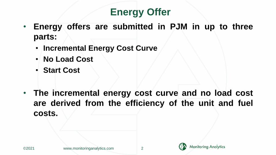
Energy Offer

• Energy offers are submitted in PJM in up to three

parts:

• Incremental Energy Cost Curve

• No Load Cost

• Start Cost

• The incremental energy cost curve and no load cost

are derived from the efficiency of the unit and fuel

costs.

©2021 www.monitoringanalytics.com 2

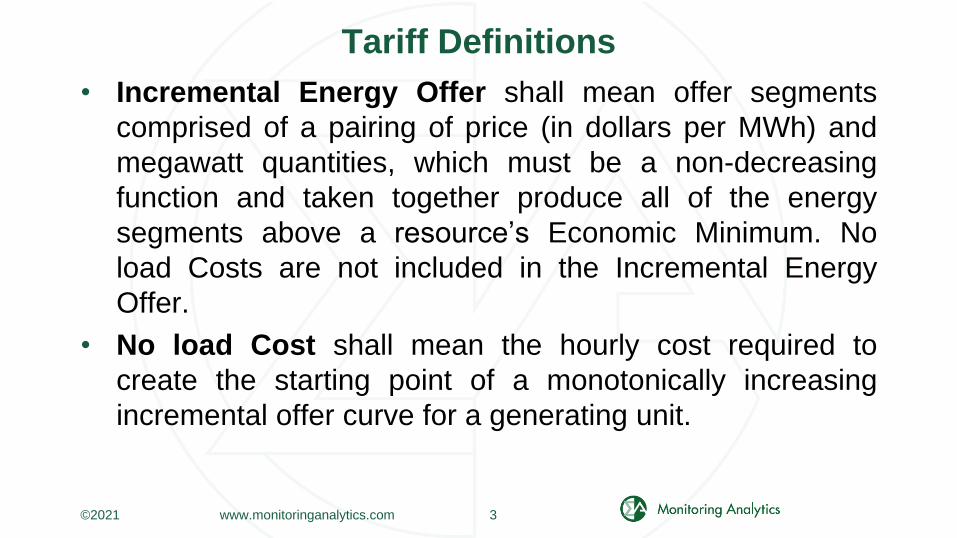
Tariff Definitions

• Incremental Energy Offer shall mean offer segments

comprised of a pairing of price (in dollars per MWh) and

megawatt quantities, which must be a non-decreasing

function and taken together produce all of the energy

segments above a resource’s Economic Minimum. No

load Costs are not included in the Incremental Energy

Offer.

• No load Cost shall mean the hourly cost required to

create the starting point of a monotonically increasing

incremental offer curve for a generating unit.


Heat Input

• The incremental energy cost curve is derived using

the incremental heat rate curve.

• The no load cost is derived using the no load heat.

• Both the incremental heat rate curve and no load heat

are derived from the heat input curve.


Heat Input Curve

• Heat input curves, also called input/output curves,

represent the amount of fuel used to produce energy.

Heat input curves are developed based on net energy

production. Heat input curves can be developed using

historical data, performance test data or Original

Equipment Manufacturer (OEM) documentation.


Heat Input Curve

• Observed fuel heat input and electric output data

during normal operation or a performance test provide

a direct measure of the heat input curve. A linear

regression of the heat input on the energy output can

provide an estimated polynomial curve. In the typical

case, the heat input curve is a second order

polynomial that applies to the entire operating output

range of the unit.

• Heat input curves are typically represented using a

second order polynomial:

𝐻(𝑀𝑊) = 𝑋2 × 𝑀𝑊2 + 𝑋1 × 𝑀𝑊 + 𝑋0


Heat Input Curve Example


0

200

400

600

800

1,000

1,200

0 10 20 30 40 50 60 70 80 90 100

Hea

t In

pu

t (M

MB

tu/h

ou

r)

Output (MW)

Data Points

Regression

Heat Input CurveH(MW) = 0.1224 X MW2 + 6.66 X MW + 310

No Load Heat

No Load Heat

• The no load heat is the estimated amount of fuel

needed to theoretically operate a unit at zero MW. The

no load heat is the constant term (X0) of the heat input

curve.

• The no load cost is equal to the no load heat (MMBtu)

times fuel cost ($/MMBtu).

• Example:

• No Load Heat = 310 MMBtu/hour

• Fuel Cost = $3/MMBtu

• No Load Cost = $930/hour


No Load Cost

• The no load cost is not a fudged number to create a

monotonically nondecreasing incremental cost curve.

• The no load cost is not the cost to get the unit to

synchronization.

• The no load cost is the hourly energy cost required to

theoretically operate a unit at zero MW (no load).


No Load Cost Equation

• No Load Cost


𝑁𝐿 = 𝐻(0) × (𝐹𝐶 + 𝑉𝑂𝑀(0) + 𝐸𝐶(0))+ 𝑉𝑂𝑀ℎ𝑜𝑢𝑟

where:

NL is the no load cost in $/hour.

H(0) is the no load heat input, the intercept of the heat input curve, in MMBtu.

FC is the fuel cost at MW output of zero, in $/MMBtu. For units that use a different starting fuel

(e.g. coal units), the fuel in the no load cost calculation cannot be the fuel used during startup and

synchronization, but must be the fuel used during normal operation.

VOM(0) is the sum of the variable operating cost and maintenance adder at zero MW, in $/MMBtu.

VOMhour is the sum of the variable operating cost and maintenance adder at zero MW, in $/hour.

EC(0) is the cost of emission credit allowances at zero MW, in $/MMBtu.

Incremental Heat Rate Curve

• The incremental heat rate curve is the change in heat

input required to produce the next MW of output. It

varies with the output level. In mathematical terms, it

is the first derivative of the heat input function. In

PJM, units can have offers based on incremental heat

rates using a sloped function or a stepped function.



• When a sloped function is used, the incremental heat

rate function is:

𝐻′ 𝑀𝑊 = 2 × 𝑋2 × 𝑀𝑊 + 𝑋1

• When a stepped function is used, the incremental heat

rate function is:

𝐻′ 𝑀𝑊𝑖 =𝐻 𝑀𝑊𝑖 − 𝐻 𝑀𝑊𝑖−1

𝑀𝑊𝑖 − 𝑀𝑊𝑖−1

• Where H(MW) is the heat input curve.




6.0

6.5

7.0

7.5

8.0

8.5

9.0

9.5

10.0

0 10 20 30 40 50 60 70 80 90 100

Incr

emen

tal H

eat

Rat

e (M

MB

tu/M

Wh

)

Output (MW)

Stepped Curve

Sloped Curve


• The shape of the offer curve (sloped or stepped) is

selected by Market Participants in Markets Gateway.

• Selecting the incorrect shape in Markets Gateway

results in:

• Understatement when incremental heat rate curve is

calculated as stepped and selected as sloped in Markets

Gateway.

• Overstatement (penalty) when incremental heat rate

curve is calculated as sloped and selected as stepped in

Markets Gateway.


Incremental Offer Curve Shapes


$0

$10

$20

$30

$40

$50

$60

$70

0 10 20 30 40 50 60 70 80 90 100

Incr

emen

tal O

ffer

($/

MW

h)

Output (MW)

Offer Points

Stepped Offer

Sloped Offer

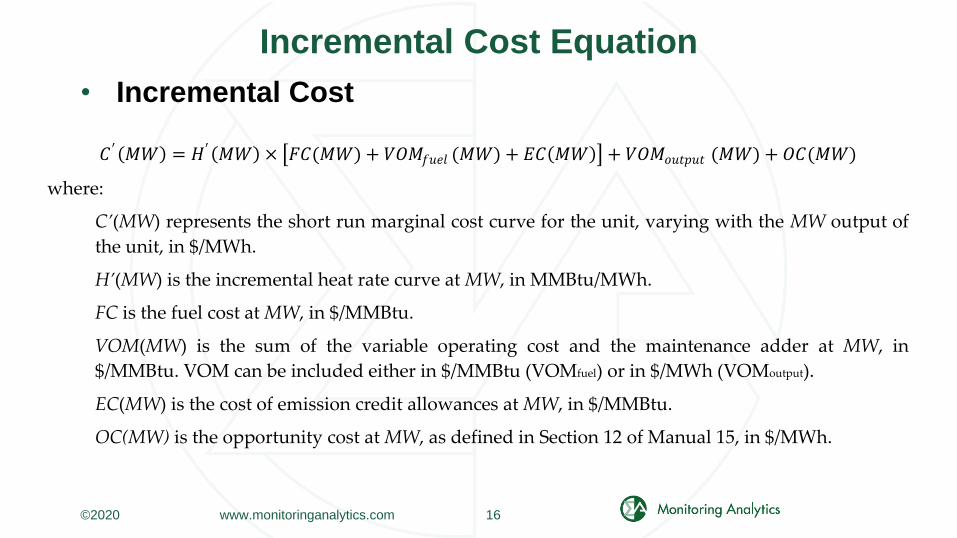
Incremental Cost Equation

• Incremental Cost


𝐶 ′(𝑀𝑊) = 𝐻′(𝑀𝑊) × 𝐹𝐶(𝑀𝑊) + 𝑉𝑂𝑀𝑓𝑢𝑒𝑙 (𝑀𝑊) + 𝐸𝐶(𝑀𝑊) + 𝑉𝑂𝑀𝑜𝑢𝑡𝑝𝑢𝑡 (𝑀𝑊) + 𝑂𝐶(𝑀𝑊)

where:

C’(MW) represents the short run marginal cost curve for the unit, varying with the MW output of

the unit, in $/MWh.

H’(MW) is the incremental heat rate curve at MW, in MMBtu/MWh.

FC is the fuel cost at MW, in $/MMBtu.

VOM(MW) is the sum of the variable operating cost and the maintenance adder at MW, in

$/MMBtu. VOM can be included either in $/MMBtu (VOMfuel) or in $/MWh (VOMoutput).

EC(MW) is the cost of emission credit allowances at MW, in $/MMBtu.

OC(MW) is the opportunity cost at MW, as defined in Section 12 of Manual 15, in $/MWh.

Manual 15 Incremental Cost Equations

• Manual 15 lacks a section covering the calculation of

incremental heat rates and incremental cost.

• Appendix is incorrect.

• Starting the sloped incremental offer curves with a

zero MW step makes the different no load calculations

in Manual 15 unnecessary.


Manual 15 No Load Cost Equations

1. Stepped:

2. Sloped if VOM is in $/MMBtu

3. Sloped if VOM is in $/ hour



• Only equation 1 is needed, even for sloped offers.

• Note: Formula needs to be updated to include hourly

VOM cost.

• Sloped offers need to be calculated and submitted

starting at zero MW.

• Multiple penalties have been assessed because

sloped offers did not start at zero MW and equation 1

was used in the no load cost calculation.



• Starting the incremental offer at eco min rather than

zero results in a overstatement of the incremental

cost.

• The no load adjustments in Manual 15 subtract from

the no load that overstatement so the total cost of the

unit is not overstated.


$0

$10

$20

$30

$40

$50

$60

$70

0 20 40 60 80 100

Incr

emen

tal O

ffer

($/

MW

h)

Output (MW)

Sloped starting at eco min

Sloped starting at zero

Block Loaded Offers

• Block loaded incremental offers are calculated using

average heat rates and not incremental heat rates.

• Average heat rate or referred just as heat rate is the

efficiency of the unit at full load.

• The average heat rate is typically calculated by adding

the total MMBtu consumed during a given period

divided by the total MWh produced during the same

period.

• It can also be calculated as the total heat input

derived from the heat input curve divided by full

output.


Block Loaded Offers

• Using this heat input curve:

• The resulting average heat rate is 10.98 MMBtu/MWh.

• Higher than the incremental heat rate curve.

• That is because block loaded offers include the entire

heat input (not just the incremental heat input above

zero MW), they include the no load heat and therefore

the no load cost.


Recommendations

• Include clear equations for incremental heat rates and

incremental offers in Manual 15.

• Include clear equations for no load cost in Manual 15.

• Allow and require the use of block loaded offers for

units that operate that way.

• Fix the tariff definitions.


MMU Cost Offer Technical Guide

• The MMU drafted a cost-based offer technical guide to

document the equations that Manual 15 is lacking.

• The purpose of the guide is to:

• Clarify existing Manual 15 (PJM Cost Development

Guideline) language.

• Provide clear equations for the calculation of accurate

cost-based offers.

• Include detailed, easy to follow examples.

• Help prevent mistakes in submitting offers for thermal

units.

• http://www.monitoringanalytics.com/reports/Technical

_References/references.shtml©2021 www.monitoringanalytics.com 24

http://www.monitoringanalytics.com/reports/Technical_References/references.shtml

Monitoring Analytics, LLC

2621 Van Buren Avenue

Suite 160

Eagleville, PA

19403

(610) 271-8050

[email protected]

www.MonitoringAnalytics.com


mailto:[email protected]

http://www.monitoringanalytics.com/

Documents

Energy Offer Calculation Education - PJM