Embed Size (px)
Citation preview

arX
iv:g
r-qc
/020
9114
v1 3
0 Se
p 20
02
OCU-PHYS-191
AP-GR-7
Energy-Momentum and Angular Momentum
Carried by Gravitational Waves in Extended New
General Relativity
Eisaku Sakane1 and Toshiharu Kawai
2,3
Department of Physics, Graduate School of Science,
Osaka City University, Osaka 558-8585, Japan
Abstract
In an extended, new form of general relativity, which is a teleparallel theory
of gravity, we examine the energy-momentum and angular momentum carried
by gravitational wave radiated from Newtonian point masses in a weak-field
approximation. The resulting wave form is identical to the corresponding
wave form in general relativity, which is consistent with previous results in
teleparallel theory. The expression for the dynamical energy-momentum den-
sity is identical to that for the canonical energy-momentum density in general
relativity up to leading order terms on the boundary of a large sphere includ-
ing the gravitational source, and the loss of dynamical energy-momentum,
which is the generator of internal translations, is the same as that of the
canonical energy-momentum in general relativity. Under certain asymptotic
conditions for a non-dynamical Higgs-type field ψk, the loss of “spin” angular
momentum, which is the generator of internal SL(2, C) transformations, is
the same as that of angular momentum in general relativity, and the losses
of canonical energy-momentum and orbital angular momentum, which con-
stitute the generator of Poincare coordinate transformations, are vanishing.
1E-mail: [email protected]: [email protected] address: 6-5-5, Onodai, Osakasayama, Osaka 589-0023, Japan.
1
The results indicate that our definitions of the dynamical energy-momentum
and angular momentum densities in this extended new general relativity work
well for gravitational wave radiations, and the extended new general relativity
accounts for the Hulse-Taylor measurement of the pulsar PSR1913+16.
1 Introduction
General relativity (GR) is a standard theory of gravity which has passed all the
observational tests so far carried out, and it constitutes, together with quantum
field theory, a basic framework of modern theoretical physics. In GR, however, it
is usually asserted [1] that well-behaved energy-momentum and angular momentum
densities cannot be defined in general for a gravitational field. For a restricted class of
systems including asymptotically flat space-time, there exist tensor densities whose
integrals over the cross section of the null infinity give the energy-momentum and
angular momentum of the system in question [2].
There are many theories [3] that are potential alternatives to GR, including the
Poincare gauge theory (PGT) [4] and extended new general relativity (ENGR) [5].
PGT is formulated on the basis of the principal fiber bundle over the space-time
possessing the covering group P0 of the proper orthochronous Poincare group as the
structure group, following the standard geometric formulation of Yang-Mills theories
as closely as possible. ENGR is formulated as the teleparallel limit of PGT. The
dynamical energy-momentum and “spin” angular momentum densities of gravita-
tional and matter fields are all space-time vector densities, and their integrations
over an arbitrary space-like surface σ are well-defined for any coordinate system
employed [6].
For asymptotically flat space-time whose vierbeins satisfy certain asymptotic
conditions,4 the integration of the dynamical energy-momentum density over σ is
the generator of internal translations and gives the total energy-momentum of the
system. Also, the integration of the “spin” angular momentum density over σ is the
generator of internal SL(2, C)-transformations and gives the total (=spin+orbital)
4With regard to the situation in ENGR, see Eqs. (2.45) and (2.46) in §2.2.
2
angular momentum in both theories. This holds in PGT when the Higgs-type field
ψk satisfies the asymptotic condition ψk = e(0)k
µxµ + ψ(0)k + O(1/rβ) with con-
stants e(0)k
µ, ψ(0)k [7, 8, 9] and in ENGR when this asymptotic condition and certain
other additional conditions are satisfied[5]. These theories describe within the un-
certainties all the observed gravitational phenomena when the parameters in the
gravitational Lagrangian densities satisfy certain conditions.
Direct observation of gravitational waves is one of the most challenging problems
in present day gravitational physics. Several projects designed for this purpose are
now being carried out, and gravitational radiations from various possible sources
have been investigated theoretically, mainly on the basis of GR. However, also in
classes of teleparallel theories of gravity, the form of gravitational waves is known
to be identical to that of GR in post-Newtonian approximations [10, 11].
For the case in which a gravitational wave is radiated, however, the asymptotic
behavior of vierbeins is different from that considered in Ref. [5] in general, and the
question of whether our definitions of the energy-momentum and angular momentum
densities work well in this case should also be answered.
The purpose of the present paper is to examine, in a weak-field approximation,
the energy-momentum and angular momentum carried by gravitational waves radi-
ated from Newtonian point masses. In §2, the basic framework of ENGR is briefly
summarized as preparation for later discussion. In §3, the forms of the gravitational
field equations and the dynamical energy-momentum density GTµ
k of the gravita-
tional field are given in the weak-field approximation. For plane wave solutions of
the linearized homogeneous equations of a gravitational field, we give the average
of GTµ
k over a space-time region much larger than the inverse of the absolute value
of the three-dimensional wave number vector. In §4, the quadrupole radiation for-
mula for a gravitational wave emitted from a system of Newtonian point masses is
obtained. In §5, we examine the emission rates of the dynamical energy-momentum
and the angular momentum for two types of the asymptotic form of a Higgs-type
field. Further, the emission rates of the canonical energy-momentum and the “ex-
tended orbital angular momentum” are examined. Finally, in §6, we give a summary
and discussion.
3
2 Basic framework of extended new general rela-
tivity
2.1 Poincare gauge theory
We first give the outline of PGT, because ENGR is formulated as a reduction of
this theory.
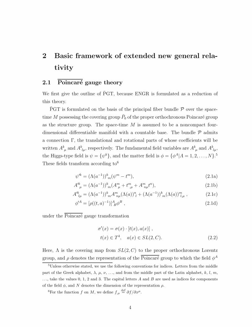
PGT is formulated on the basis of the principal fiber bundle P over the space-
timeM possessing the covering group P0 of the proper orthochronous Poincare group
as the structure group. The space-time M is assumed to be a noncompact four-
dimensional differentiable manifold with a countable base. The bundle P admits
a connection Γ, the translational and rotational parts of whose coefficients will be
written Akµ and Ak
lµ, respectively. The fundamental field variables are Akµ and Ak
lµ,
the Higgs-type field is ψ = ψk, and the matter field is φ = φA|A = 1, 2, . . . , N.5
These fields transform according to6
ψ′k = (Λ(a−1))km(ψm − tm), (2.1a)
A′kµ = (Λ(a−1))km(A
mµ + tm,µ + Am
nµtn), (2.1b)
A′klµ = (Λ(a−1))kmA
mnµ(Λ(a))
nl + (Λ(a−1))km(Λ(a))
ml,µ , (2.1c)
φ′A = [ρ((t, a)−1)]ABφB , (2.1d)
under the Poincare gauge transformation
σ′(x) = σ(x) · [t(x), a(x)] ,t(x) ∈ T 4, a(x) ∈ SL(2, C). (2.2)
Here, Λ is the covering map from SL(2, C) to the proper orthochronous Lorentz
group, and ρ denotes the representation of the Poincare group to which the field φA
5Unless otherwise stated, we use the following conventions for indices. Letters from the middle
part of the Greek alphabet, λ, µ, ν, . . ., and from the middle part of the Latin alphabet, k, l, m,
. . ., take the values 0, 1, 2 and 3. The capital letters A and B are used as indices for components
of the field φ, and N denotes the dimension of the representation ρ.
6For the function f on M , we define f,µdef= ∂f/∂xµ.
4
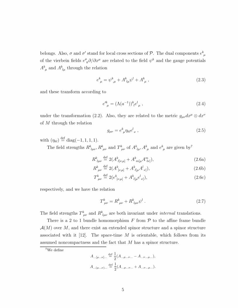
belongs. Also, σ and σ′ stand for local cross sections of P. The dual components ekµ
of the vierbein fields eµk∂/∂xµ are related to the field ψk and the gauge potentials
Akµ and Ak
lµ through the relation
ekµ = ψk,µ + Ak
lµψl + Ak
µ , (2.3)
and these transform according to
e′kµ = (Λ(a−1))klelµ , (2.4)
under the transformation (2.2). Also, they are related to the metric gµνdxµ ⊗ dxν
of M through the relation
gµν = ekµηklelν , (2.5)
with (ηkl)def= diag(−1, 1, 1, 1).
The field strengths Rklµν , R
kµν and T k
µν of Aklµ, A
kµ and ekµ are given by7
Rklµν
def= 2(Ak
l[ν,µ] + Akm[µA
mlν]), (2.6a)
Rkµν
def= 2(Ak
[ν,µ] + Akl[µA
lν]), (2.6b)
T kµν
def= 2(ek[ν,µ] + Ak
l[µelν]), (2.6c)
respectively, and we have the relation
T kµν = Rk
µν +Rklµνψ
l . (2.7)
The field strengths T kµν and Rk
lµν are both invariant under internal translations.
There is a 2 to 1 bundle homomorphism F from P to the affine frame bundle
A(M) over M , and there exist an extended spinor structure and a spinor structure
associated with it [12]. The space-time M is orientable, which follows from its
assumed noncompactness and the fact that M has a spinor structure.
7We define
A...[µ...ν]...def=
1
2(A...µ...ν... −A...ν...µ...),
A...(µ...ν)...def=
1
2(A...µ...ν... +A...ν...µ...).
5

The affine frame bundle A(M) admits a connection ΓA. The T4 part Γµ
ν and the
GL(4, R) part Γλµν of its connection coefficients are related to Ak
lµ and ekµ through
the relations
Γµν = δµν , (2.8a)
Aklµ = ekλe
νlΓ
λνµ + ekνe
νl,µ , (2.8b)
by the requirement that F maps the connection Γ into ΓA, and the space-time M
is of the Riemann-Cartan type.
The torsion is given by
T λµν
def= 2Γλ
[νµ] , (2.9)
and the T 4 and GL(4, R) parts of the curvature are given by
Rλµν = 2(Γλ
[ν,µ] + Γλρ[µΓ
ρ
ν]), (2.10)
Rλρµν = 2(Γλ
ρ[ν,µ] + Γλτ [µΓ
τρν]), (2.11)
respectively. Then, we have the relations
T kµν = ekλT
λµν = ekλR
λµν , (2.12)
Rklµν = ekλe
ρlR
λρµν , (2.13)
which follow from Eq. (2.8).
The covariant derivative of the matter field φ takes the form
DkφA = eµkDµφ
A , (2.14)
DµφA def= ∂µφ
A +i
2Akl
µ(Mklφ)A + iAk
µ(Pkφ)A , (2.15)
whereMkl and Pk are representation matrices of the standard basis of the Lie algebra
of the group P0: Mkl = −iρ∗(Mkl), Pk = −iρ∗(Pk). The matrix Pk represents the
“intrinsic energy-momentum” of the field φA [12], and it is vanishing for all observed
fields.
6
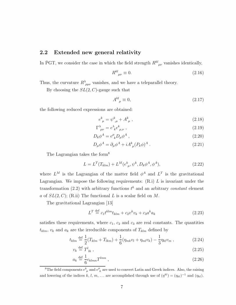
2.2 Extended new general relativity
In PGT, we consider the case in which the field strength Rklµν vanishes identically,
Rklµν ≡ 0. (2.16)
Thus, the curvature Rλρµν vanishes, and we have a teleparallel theory.
By choosing the SL(2, C)-gauge such that
Aklµ ≡ 0, (2.17)
the following reduced expressions are obtained:
ekµ = ψk,µ + Ak
µ , (2.18)
Γλµν = eλke
kµ,ν , (2.19)
DkφA = eµkDµφ
A , (2.20)
DµφA = ∂µφ
A + iAkµ(Pkφ)
A . (2.21)
The Lagrangian takes the form8
L = LT (Tklm) + LM(ekµ, ψk, Dkφ
A, φA), (2.22)
where LM is the Lagrangian of the matter field φA and LT is the gravitational
Lagrangian. We impose the following requirements: (R.i) L is invariant under the
transformation (2.2) with arbitrary functions tk and an arbitrary constant element
a of SL(2, C); (R.ii) The functional L is a scalar field on M .
The gravitational Lagrangian [13]
LT def= c1t
klmtklm + c2vkvk + c3a
kak (2.23)
satisfies these requirements, where c1, c2 and c3 are real constants. The quantities
tklm, vk and ak are the irreducible components of Tklm defined by
tklmdef=
1
2(Tklm + Tlkm) +
1
6(ηmkvl + ηmlvk)−
1
3ηklvm , (2.24)
vkdef= T l
lk , (2.25)
akdef=
1
6ǫklmnT
lmn , (2.26)
8The field components ekµ and eµk are used to convert Latin and Greek indices. Also, the raising
and lowering of the indices k, l, m, . . . are accomplished through use of (ηkl) = (ηkl)−1 and (ηkl).
7

where the symbol ǫklmn represents the Levi-Civita tensor, with ǫ(0)(1)(2)(3) = −1.9
If the parameters c1, c2 and c3 satisfy
c1 = −c2 =4
9c3 = − 1
3κ, (2.27)
where κ is the Einstein gravitational constant, κdef= 8πG/c4,10 the gravitational part
of the action integral is equal to the Einstein-Hilbert action integral, namely [13]
∫d4x
√−gLT =
∫d4x
1
2κ
√−gR(), (2.28)
where R() denotes the Riemann-Christoffel scalar curvature. Here, we should
mention that even in the case that the condition (2.27) is satisfied, our theory
does not reduce to GR, because the couplings of matter fields (the spinor field, for
example) with the gravitational field are different from those in GR.
In defining the energy-momentum and angular momentum, there are two pos-
sibilities for choosing the set of independent field variables [5, 7, 8, 9]: One is to
choose the set ψk, Akµ, φ
A, and the other is to choose the set ψk, ekµ, φA. In the
rest of this paper, we employ ψk, Akµ, φ
A as the set of independent field variables,
because this choice is superior to the other, as shown in Refs. [5, 7, 8, 9].
From the requirement (R.i), we obtain the identities11
δL
δψk+ ∂µ
(δL
δAkµ
)+ i
δL
δφA(Pkφ)
A ≡ 0, (2.29)
F(µν)
k ≡ 0, (2.30)
totTµ
k − ∂νFµν
k − δL
δAkµ
≡ 0, (2.31)
∂µtotS
µkl − 2
δL
δψ[kψl] − 2
δL
δA[kµ
Al]µ − iδL
δφA(Mklφ)
A ≡ 0, (2.32)
9 Latin indices are put in parentheses to distinguish them from Greek indices.10G and c stand for the Newtonian gravitational constant and the light velocity in vacuum,
respectively.11For instance, δL/δψk denotes the Euler derivative with respect to ψk.
8
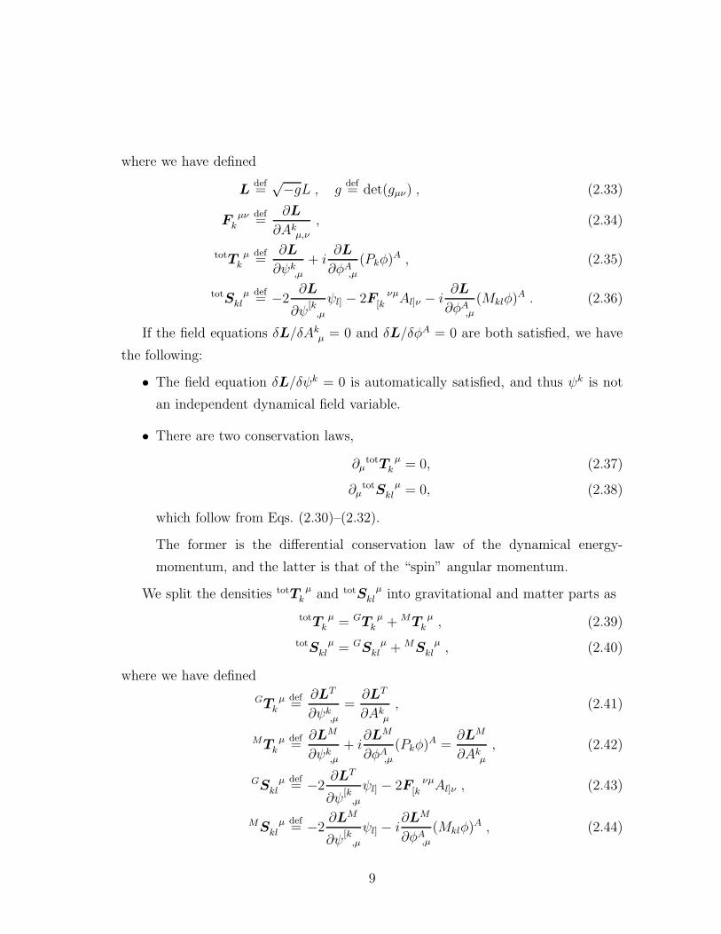
where we have defined
Ldef=
√−gL , gdef= det(gµν) , (2.33)
Fµν
k
def=
∂L
∂Akµ,ν
, (2.34)
totTµ
k
def=
∂L
∂ψk,µ
+ i∂L
∂φA,µ
(Pkφ)A , (2.35)
totSµ
kl
def= −2
∂L
∂ψ[k,µ
ψl] − 2F νµ
[k Al]ν − i∂L
∂φA,µ
(Mklφ)A . (2.36)
If the field equations δL/δAkµ = 0 and δL/δφA = 0 are both satisfied, we have
the following:
• The field equation δL/δψk = 0 is automatically satisfied, and thus ψk is not
an independent dynamical field variable.
• There are two conservation laws,
∂µtotT
µk = 0, (2.37)
∂µtotS
µkl = 0, (2.38)
which follow from Eqs. (2.30)–(2.32).
The former is the differential conservation law of the dynamical energy-
momentum, and the latter is that of the “spin” angular momentum.
We split the densities totTµ
k and totSµ
kl into gravitational and matter parts as
totTµ
k = GTµ
k + MTµ
k , (2.39)
totSµ
kl = GSµ
kl + MSµ
kl , (2.40)
where we have defined
GTµ
k
def=
∂LT
∂ψk,µ
=∂LT
∂Akµ
, (2.41)
MTµ
k
def=
∂LM
∂ψk,µ
+ i∂LM
∂φA,µ
(Pkφ)A =
∂LM
∂Akµ
, (2.42)
GSµ
kl
def= −2
∂LT
∂ψ[k,µ
ψl] − 2F νµ
[k Al]ν , (2.43)
MSµ
kl
def= −2
∂LM
∂ψ[k,µ
ψl] − i∂LM
∂φA,µ
(Mklφ)A , (2.44)
9

with LT def=
√−gLT and LM def=
√−gLM . Here, GTµ
k and MTµ
k are the dynamical
energy-momentum densities of the gravitational field and the matter field, respec-
tively, while GSµ
kl and MSµ
kl are the “spin” angular momentum densities of the
gravitational field and the matter field, respectively. The densities GTµ
k ,MTµ
k ,GS
µkl and MS
µkl are all space-time vector densities [6].
In Ref. [5], the integrals of the dynamical energy-momentum and “spin” angular
momentum densities over a space-like surface σ are examined for vierbeins with the
asymptotic behavior described below.
〈1〉 The components ekµ of the vierbein fields possess the asymptotic property12
ekµ = e(0)kµ + fkµ , fk
µ,(m) = O(1/r1+m) (m = 0, 1, 2), (2.45)
where fkµ,(m) denotes the mth order partial derivative with respect to xλ, and the
e(0)k
µ are constant vierbeins satisfying e(0)k
µηkle(0)l
ν = ηµν .
〈2〉 The antisymmetric part of components fµνdef= e
(0)kµηklf
lν satisfy
f[µν],(m) = O(1/r1+α+m) (m = 0, 1), (2.46)
where α is positive but otherwise arbitrary.
It has been shown that
Mkdef=
∫
σ
totTµ
k dσµ = e(0)µ
kMµ , (2.47)
Skldef=
∫
σ
totSµ
kl dσµ = e(0)
kµe(0)
lνMµν + 2ψ
(0)[kMl] , (2.48)
where dσµ denotes the surface element on σ. In the above, we have defined
Mµdef= ηµν
∫
σ
θνλdσλ (2.49)
Mµν def=
∫
σ
∂ρKµνλρdσλ =
∫
σ
(xµθνλ − xνθµλ)dσλ , (2.50)
12The expression O(1/rn) with real n denotes a term for which rnO(1/rn) remains finite for
r → ∞; a term denoted as O(1/rn) could, of course, also be zero.
10
with
θνλdef=
1
κ∂ρ∂σ(−g)gν[λgρ]σ, (2.51)
Kµνλρ def=
1
κ
(xµ∂σ(−g)gν[λgρ]σ − xν∂σ(−g)gµ[λgρ]σ+ (−g)gµ[λgρ]ν − ηµ[ληρ]ν
).
(2.52)
This expression of θνλ is the same as that of the symmetric energy-momentum
density proposed by Landau and Lifshitz [14]. Equation (2.48) has been obtained
by choosing the asymptotic form of the Higgs-type field ψk as
ψk = e(0)kµxµ + ψ(0)k +O
(1
rβ
), (2.53a)
ψk,µ = e(0)kµ +O
(1
r1+β
), (β > 0) (2.53b)
ψk,µν = O
(1
r2
), (2.53c)
with ψ(0)k and β constant, whereas Eq. (2.47) has been obtained without imposing
the conditions (2.53).
From the requirement (R.ii), we obtain the identity
T νµ − ∂λΨ
νλµ − δL
δAkν
Akµ ≡ 0, (2.54)
with
T νµ
def= δ ν
µ L− F λνk Ak
λ,µ −∂L
∂φA,ν
φA,µ −
∂L
∂ψk,ν
ψk,µ , (2.55)
Ψ νλµ
def= F νλ
k Akµ = −Ψ λν
µ . (2.56)
The identity (2.54) leads to
∂νTν
µ = 0, (2.57)
∂λMνλ
µ = 0 (2.58)
when δL/δAkν = 0, where we have defined
M νλµ
def= 2(Ψ νλ
µ − xνT λµ ). (2.59)
11

Equations (2.57) and (2.58) are the differential conservation laws of the canonical
energy-momentum and the “extended orbital angular momentum” defined by
M cµ
def=
∫
σ
T νµ dσν , L ν
µ
def=
∫
σ
M νλµ dσλ , (2.60)
respectively [5]. The canonical energy-momentum and the “extended orbital angular
momentum” are the generators of general affine coordinate transformations. The
antisymmetric part L[µν]def= L λ
[µ ηλν] is the orbital angular momentum13 and is the
generator of coordinate Lorentz transformation [5].
We split the canonical energy-momentum density into gravitational and matter
parts as
T νµ = GT ν
µ + MT νµ , (2.61)
where we have defined
GT νµ
def= δ ν
µ LT − F λνk Ak
λ,µ −∂LT
∂ψk,ν
ψk,µ , (2.62)
MT νµ
def= δ ν
µ LM − ∂LM
∂ψk,ν
ψk,µ −
∂LM
∂φA,ν
φA,µ . (2.63)
The density GT νµ does not transform as a tensor density under general coordinate
transformations, while MT νµ does transform as a tensor density.[6]
As is described in Ref. [5], the generators M cµ and L ν
µ vanish for vierbeins with
the asymptotic forms satisfying Eqs. (2.45) and (2.46) when the condition (2.53) is
satisfied.
The field equation δL/δAkµ = 0 has the expression
−2∇λFµνλ + 2vλF
µνλ + 2Hµν − gµνLT = T µν , (2.64)
where we have defined
∇λFµνλ def
= ∂λFµνλ + Γµ
σλFσνλ + Γν
σλFµσλ + Γλ
σλFµνσ , (2.65)
F µνλ def= c1(t
µνλ − tµλν) + c2(gµνvλ − gµλvν)− 1
3c3ǫ
µνλρaρ , (2.66)
Hµν def= T ρσµF ν
ρσ − 1
2T νρσF µ
ρσ . (2.67)
13This L[µν] should not be confused with the orbital part of the “spin” angular momentum Skl.
12

Also, T µν is the energy-momentum density of the gravitational source defined by
√−gT µν def= ηkleµl
δLM
δAkν
. (2.68)
3 Weak-field approximation
We now consider weak field situations in which the vierbein fields ekµ take the form
ekµ = e(0)kµ + fkµ , |fk
µ| ≪ 1, (3.1)
where the e(0)k
µ are constant vierbeins satisfying e(0)k
µηkle(0)l
ν = ηµν . The compo-
nents of the metric and torsion tensors are given by, up to terms linear in fkµ,
gµν = ηµν + 2f(µν) , (3.2)
Tλµν = ∂µfλν − ∂νfλµ , (3.3)
where we have defined fµνdef= e
(0)kµηklf
lν .
14
In the weak-field approximation, the symmetric and antisymmetric parts of the
field equation (2.64) take the form
3c1f(µν) − ∂λ(∂µf(νλ) + ∂ν f(µλ)) + ηµν∂ρ∂σf
(ρσ)
+ (c1 + c2)−ηµνf − 2ηµν∂ρ∂σf
(ρσ) + ∂µ∂ν f
+ ∂λ(∂µf(νλ) + ∂ν f(µλ))− ∂λ(∂µf[νλ] + ∂νf[µλ])= T(µν) , (3.4)
(c1 −
4
9c3
)f[µν] + ∂λ(∂µf[νλ] − ∂νf[µλ])
+ (c1 + c2)∂λ(∂µf(νλ) − ∂ν f(µλ))− ∂λ(∂µf[νλ] − ∂νf[µλ])
= T[µν] , (3.5)
with def= ∂µ∂µ. Here, we have introduced
f(µν)def= f(µν) −
1
2ηµνf , f
def= ηµνf(µν) , (3.6)
fdef= ηµν f(µν) . (3.7)
14For fkµ, we use the convention that both the Greek and Latin indices of fk
µ are raised or
lowered with the Minkowski metric, and that they are converted into one another with e(0)k
µ or
e(0)µ
k, where (e(0)µ
k)def= (e
(0)kµ)−1. Thus, fµν , for example, represents ηνλe
(0)µkf
kλ(6= gνλeµkf
kλ).
13

We consider the energy-momentum density of the source Tµν to lowest order in
fkµ. Therefore it is independent of f
kµ and satisfies the ordinary conservation law in
special relativity,
∂νTµν = 0. (3.8)
Let us consider the transformations
f ′
(µν) = f(µν) − ∂µεν − ∂νεµ , (3.9)
f ′
[µν] = f[µν] + ∂µχν − ∂νχµ , (3.10)
where εµ and χµ are arbitrary small functions. Since Eqs. (3.4) and (3.5) are in-
variant under the transformations (3.9) and (3.10) with εµ = χµ, we can impose the
harmonic coordinate condition
∂ν f(µν) = 0. (3.11)
The Lagrangian LT with the parameters c1 and c2 satisfying
c1 = −c2 = − 1
3κ(3.12)
compares quite favorably with experiment [13]. We therefore assume (3.12) to hold
henceforth. Under the conditions (3.11) and (3.12), Eq. (3.5) reduces to(c1 −
4
9c3
)f[µν] + ∂λ(∂µf[νλ] − ∂νf[µλ])
= T[µν] , (3.13)
which is still invariant under the transformation (3.10) [13]. Thus, we can impose
the condition
∂νf[µν] = 0. (3.14)
Finally, under the conditions (3.11), (3.12) and (3.14), the field equations of f(µν)
and f[µν] become
f(µν) = −κT(µν) , (3.15)
f[µν] = −λT[µν] , (3.16)
where we have defined 1/λdef= −c1 + (4/9)c3 6= 0. From Eqs. (3.11) and (3.15), we
find that the symmetric part of Tµν satisfies the conservation law
∂νT(µν) = 0, (3.17)
14
and the antisymmetric part of Tµν satisfies
∂νT[µν] = 0, (3.18)
which follows from Eqs. (3.14) and (3.16) [13].
Let us consider the plane wave solutions of Eqs. (3.15) and (3.16) with Tµν ≡ 0,
f(µν)(x, x0) = Uµνe
ik·x + Uµνe−ik·x , (3.19)
f[µν](x, x0) = Vµνe
ik·x + Vµνe−ik·x , (3.20)
where k · x def= kµx
µ. Here, Uµν and Vµν are constant amplitudes, U and V are their
complex conjugates, and kµ is a constant wave vector, which satisfy the relations
kµkµ = 0, Uµνk
ν = 0, Vµνkν = 0. (3.21)
Following the prescription given in Section 35.4 of Ref. [1], we impose the transverse-
traceless gauge condition
Uµνζν = 0, Uµ
µ = 0, Vµνζν = 0, (3.22)
where ζµ is a constant time-like vector. We see that the number of physically
significant components of f(µν) is two, while that of f[µν] is one.
We next calculate the energy-momentum of the plane waves given by Eqs. (3.19)
and (3.20). The dynamical energy-momentum density GTµ
l of gravitational field
15
has, to lowest order in fµν , the expression
2κ GTµ
l = e(0)µ
l
[−∂σ f (λρ)∂σ f(λρ) + ∂σ f (λρ)∂ρf(λσ) +
1
2∂σf∂σf + 2∂σ f (λρ)∂ρf[λσ]
+ ∂λf [σρ]∂ρf[λσ] −κ
λ
(∂σf [λρ]∂σf[λρ] + 2∂λf [σρ]∂ρf[λσ]
)]
− 2e(0)ν
l
[−∂µf (ρσ)∂ν f(ρσ) +
1
2∂µf∂ν f − ∂σ f (ρµ)∂σf(ρν) + ∂σf (ρµ)∂ν f(ρσ)
+ ∂µf (ρσ)∂σf(ρν) +1
2∂σ f (ρµ)ηρν∂σf − 1
2∂µf(νσ)∂
σf − ∂σ f (ρµ)∂σf[ρν]
+ ∂σ f (ρµ)∂νf[ρσ] + ∂µf (ρσ)∂σf[ρν] + ∂σf [ρµ]∂ν f(ρσ) − ∂ρf [σµ]∂σ f(ρν)
+1
2∂νf
[σµ]∂σf − ∂σf [ρµ]∂νf[ρσ] − ∂ρf [σµ]∂σf[ρν]
− κ
λ
(∂σf [ρµ]∂σf(ρν) − ∂µf [ρσ]∂σf(ρν) − ∂ρf [σµ]∂σf(ρν)
− 1
2∂σf [ρµ]ηρν∂σ f +
1
2∂µf[νσ]∂
σ f +1
2∂νf
[σµ]∂σ f + ∂σf [ρµ]∂σf[ρν]
− 2∂σf [ρµ]∂νf[ρσ] − ∂µf [ρσ]∂σf[ρν] + ∂µf [ρσ]∂νf[ρσ]
− ∂ρf [σµ]∂σf[ρν]
)]. (3.23)
By using Eqs. (3.19)–(3.22), GTµ
l is found to be given by
GTµ
l = −2e(0)ν
l
[kµkν2κ
(UρσUρσe
2ik·x − 2UρσUρσ + UρσUρσe−2ik·x
)
+kµkν2λ
(VρσVρσe
2ik·x − 2VρσVρσ + VρσVρσe−2ik·x
)]. (3.24)
Taking the average of GTµ
l over a space-time region much larger than |k|−1, we
obtain
〈GT µl 〉 = e
(0)νl
[c4kµkν2πG
(|U11|2 + |U12|2
)+ 4
kµkνλ
|V12|2], (3.25)
where we have chosen the direction of the space components k of the four vector kµ
as the third axis. The term in the square brackets of the right-hand side (r.h.s.) of
Eq. (3.25) is identical to the corresponding term of the canonical energy-momentum
density t µν defined by Eq. (A.7) in GR if the antisymmetric part V12 is vanishing.
15
15See, for instance, Section 10.3 of Ref. [15]
16

4 Quadrupole radiation from point masses
The retarded solutions of Eqs. (3.15) and (3.16) are given by
f(µν)(x, x0) =
κ
4π
∫d3x′
T(µν)(x′, x0 − |x− x′|)|x− x′| , (4.1)
f[µν](x, x0) =
λ
4π
∫d3x′
T[µν](x′, x0 − |x− x′|)|x− x′| , (4.2)
respectively. We consider a system of the Newtonian point masses ma, ξµa (a =
1, 2, . . . , N) as a gravitational wave source, where ma and ξµa denote the mass and
coordinate of the ath point mass, respectively. For this case, the antisymmetric part
of the energy-momentum density becomes
T[µν](x, x0) = 0. (4.3)
Thus, f[µν] vanishes, i.e., f[µν] = 0. Applying the retarded expansion to Eq. (4.1)
and using the conservation law (3.17), we obtain the quadrupole radiation formula
in the rest frame of the system,
f(αβ)(x, x0) =
κ
8πr∂0∂0
∫d3x′x′αx′βT(00)(x
′, x0 − r), (4.4a)
f(0α)(x, x0) = −x
β
rf(αβ)(x
′, x0 − r), (4.4b)
f(00)(x, x0) =
κ
4πr
N∑
a=1
mac2 +
xαxβ
r2f(αβ)(x
′, x0 − r), (4.4c)
with r = (xαxα)1
2 .16 Since we regard each velocity of the mass points to be much
smaller than the velocity of light, we can use the quantity
T(00)(x, x0) =
N∑
a=1
mac2δ(3)(x− ξa(t)) (4.5)
16In our convention, letters from the beginning of the Greek alphabet, α, β, γ, · · · , and those
from the beginning of the Latin alphabet, a, b, c, · · · , take the values 1, 2, and 3, unless otherwise
stated. Also, here we have used the usual summation convention for repeated indices.
17
as the energy density of the system, with tdef= x0/c. Substituting Eq. (4.5) into
Eq. (4.4), we obtain
f(αβ) =κ
8πrDαβ , f(0α) = −x
β
r
κ
8πrDαβ , (4.6a)
f(00) =κ
4πr
N∑
a=1
mac2 +
xαxβ
r2κ
8πrDαβ . (4.6b)
Here, Dαβ is the quadrupole moment of the mass distribution defined by
Dαβdef=
N∑
a=1
maξαa ξ
βa , (4.7)
where we have defined Dαβdef= ∂2Dαβ/∂
2t. The wave form given by Eqs. (4.6) and
(4.7) is the same as the corresponding wave form in GR, which is consistent with
the result given in Ref. [11].
5 Emission rates of energy-momentum and angu-
lar momentum
In this section, we examine time averages of emission rates of the energy-momentum
and angular momentum carried by the quadrupole radiation given by Eq. (4.6).
In ENGR, for the asymptotic conditions (2.45) and (2.46), we have four quantities
that are conserved as long as they are finite, the dynamical energy-momentum Mk,
“spin” angular momentum Skl, canonical energy-momentum M cµ, and “extended
orbital angular momentum” L νµ [5]. The dynamical energy momentum does not
depend on the asymptotic form of the Higgs-type field ψk explicitly, but the quantities
Skl,Mcµ and L ν
µ depend on the asymptotic form. With this in mind, following
Ref. [5], we examine the case in which the asymptotic form of the Higgs-type field
is
ψk ≃ e(0)kµxµ + ψ(0)k ,
with ψ(0)k constant. We also consider the slightly generalized case in which
ψk ≃ ρe(0)kµxµ + ψ(0)k.
The asymptotic form of the function ρ is determined in §5.2.
18

5.1 The case ψk ≃ e(0)k
µxµ + ψ(0)k
5.1.1 Dynamical energy-momentum loss
In order to evaluate the emission rate of the dynamical energy-momentum, we inte-
grate the differential conservation law (2.37) over a large solid sphere V with radius
r, yielding
∂0
∫
V
totT 0k d
3x = −∫
S
totT αk r2nαdΩ , (5.1)
where S and dΩ represent the two-dimensional surface of V and the differential solid
angle, respectively. Also, nα stands for the unit radial vector defined by nα def= xα/r.
Taking into account the fact that the energy-momentum density of point masses
vanishes for very large r, we can rewrite the r.h.s. of Eq. (5.1) as
−∫
S
totT αk r2nαdΩ = −
∫
S
GT αk r2nαdΩ . (5.2)
The density GTµ
k takes, up to terms of order O(1/r2), the form
GTµ
k = e(0)ν
kGT (0) µ
ν , (5.3)
withGT (0) µ
ν
def=
1
κ
(∂µf (ρσ)∂ν f(ρσ) −
1
2∂µf∂ν f
). (5.4)
Using the solution (4.6), and averaging over one period of motion of the system of
point masses, we obtain
−⟨dE
dt
⟩=
G
5c5
⟨...Dαβ
...Dαβ −
1
3
...Dαα
...Dββ
⟩, (5.5)
for a total energy Edef= −M(0) of the system, where 〈· · · 〉 denotes the operation of
averaging over one period of motion of the system of the point masses, and we have
set e(0)k
µ = δkµ for simplicity. Also, we obtain
dMa
dt= 0. (5.6)
It is worth mentioning that the quantity GT(0) ν
µ is identical to the r.h.s. of Eq. (A.14),
and the time average of the emission rate of the dynamical energy-momentum,
which is given by Eqs. (5.5) and (5.6), is identical to that of the canonical energy-
momentum in GR.
19

5.1.2 “Spin” angular momentum loss
The density GSµ
kl has the expression
GSµ
kl = 2ηkmηlne(0)m
[ρe(0)n
σ]ψρ(−g)tσµLL
− 2e(0)ν
[kηl]me(0)m
τ
[Z(1) µ
ν ψτ + ηνσ(Z
(2)µστ − Z(3)µλσψτ,λ)
],
(5.7)
where we have defined
ψρ def= e
(0)ρkψ
k , (5.8)
κZ(1) µν
def= −1
2δ µν ∂
σ f (λρ)∂ρf(λσ) − ∂σ f (ρµ)∂σf(ρν) + ∂σ f (ρµ)∂ν f(ρσ)
+ ∂µf (ρσ)∂σf(ρν) −1
2∂σ f (ρµ)ηρν∂σf +
1
2∂µf(νσ)∂
σ f , (5.9)
κZ(2)µστ def=
(∂λf (σµ) − ∂µf (σλ)
)(δτλ + ητρf(ρλ) −
1
2δτλf
), (5.10)
κZ(3)µλσ def= ∂λf (σµ) − ∂µf (σλ) . (5.11)
Also, tσµLL denotes the energy-momentum density introduced by Landau and Lifshitz,
whose explicit form is given in Appendix A. Using a method similar to that employed
in §5.1.1, we obtain
∂0
∫
V
totS 0kl d
3x = −∫
S
GS αkl r
2nαdΩ . (5.12)
In order to estimate the r.h.s. of Eq. (5.12), we set
ψµ = xµ + ψ(0)µ + ψµ , (5.13)
where ψ(0)µ is a constant. From Eqs. (4.6) and (5.7)–(5.13), we can show that17
−⟨dS(0)a
dt
⟩= −ψ(0)a G
5c6
⟨...Dαβ
...Dαβ −
1
3
...Dαα
...Dββ
⟩
= −2ψ(0)
[a
⟨dM(0)]
dt
⟩(5.14)
17Note that we have distinguished between Latin and Greek indices here. (See footnote 9 on
page 8.)
20
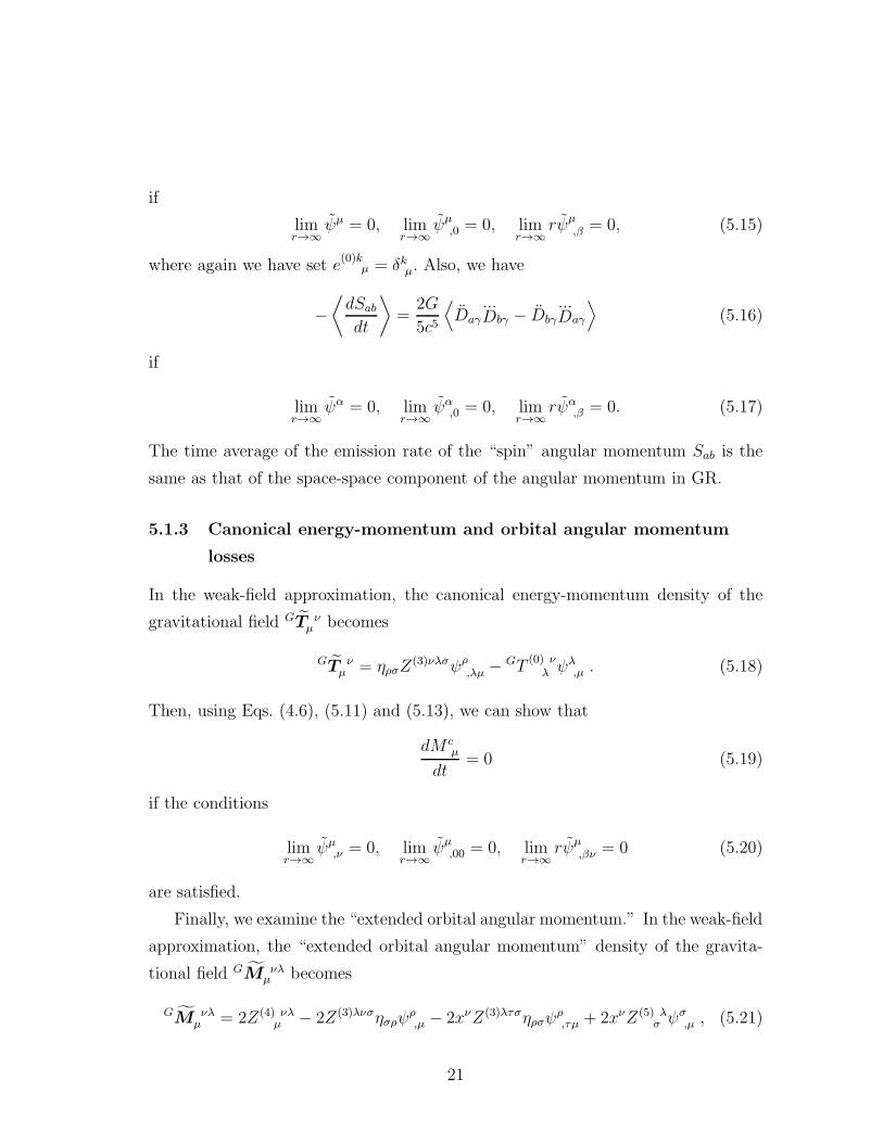
if
limr→∞
ψµ = 0, limr→∞
ψµ,0 = 0, lim
r→∞
rψµ,β = 0, (5.15)
where again we have set e(0)k
µ = δkµ. Also, we have
−⟨dSab
dt
⟩=
2G
5c5
⟨Daγ
...Dbγ − Dbγ
...Daγ
⟩(5.16)
if
limr→∞
ψα = 0, limr→∞
ψα,0 = 0, lim
r→∞
rψα,β = 0. (5.17)
The time average of the emission rate of the “spin” angular momentum Sab is the
same as that of the space-space component of the angular momentum in GR.
5.1.3 Canonical energy-momentum and orbital angular momentum
losses
In the weak-field approximation, the canonical energy-momentum density of the
gravitational field GT νµ becomes
GT νµ = ηρσZ
(3)νλσψρ,λµ − GT
(0) ν
λ ψλ,µ . (5.18)
Then, using Eqs. (4.6), (5.11) and (5.13), we can show that
dM cµ
dt= 0 (5.19)
if the conditions
limr→∞
ψµ,ν = 0, lim
r→∞
ψµ,00 = 0, lim
r→∞
rψµ,βν = 0 (5.20)
are satisfied.
Finally, we examine the “extended orbital angular momentum.” In the weak-field
approximation, the “extended orbital angular momentum” density of the gravita-
tional field GM νλµ becomes
GM νλµ = 2Z(4) νλ
µ − 2Z(3)λνσησρψρ,µ − 2xνZ(3)λτσηρσψ
ρ,τµ + 2xνZ(5) λ
σ ψσ,µ , (5.21)
21
where we have defined
κZ(4) νλµ
def=
(∂ν f (σλ) − ∂λf (σν)
)(ησµ + f(σµ) −
1
2ησµf
)
+ xν[δ λµ
(1
2∂σ f (τρ)∂σf(τρ) −
1
2∂σ f (τρ)∂ρf(τσ) −
1
4∂σf∂σf
)
+(∂ρf (σλ) − ∂λf (σρ)
)(∂µf(σρ) −
1
2ησρ∂µf
)], (5.22)
κZ(5) λσ
def= δ λ
σ
(−1
2∂ξf (τρ)∂ξf(τρ) +
1
2∂ξf (τρ)∂ρf(τξ) +
1
4∂ρf∂ρf
)
+ ∂λf (ρτ)∂σf(ρτ) −1
2∂λf∂σf + ∂τ f (ρλ)∂τ f(ρσ) − ∂τ f (ρλ)∂σf(ρτ)
− ∂λf (ρτ)∂τ f(ρσ) −1
2∂τ f (ρλ)ηρσ∂τ f +
1
2∂λf(στ)∂
τ f . (5.23)
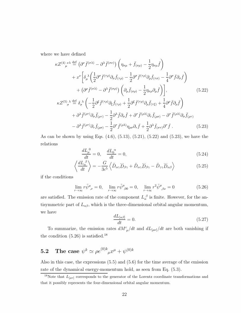
As can be shown by using Eqs. (4.6), (5.13), (5.21), (5.22) and (5.23), we have the
relations
dL 0µ
dt= 0,
dL α0
dt= 0, (5.24)
⟨dL β
α
dt
⟩= − G
3c5
⟨Dαγ
...Dβγ + Dαγ
...Dβγ − Dγγ
...Dαβ
⟩(5.25)
if the conditions
limr→∞
rψµ,ν = 0, lim
r→∞
rψµ,00 = 0, lim
r→∞
r2ψµ,βν = 0 (5.26)
are satisfied. The emission rate of the component L βα is finite. However, for the an-
tisymmetric part of Lαβ , which is the three-dimensional orbital angular momentum,
we havedL[αβ]
dt= 0. (5.27)
To summarize, the emission rates dM cµ/dt and dL[µν]/dt are both vanishing if
the condition (5.26) is satisfied.18
5.2 The case ψk ≃ ρe(0)k
µxµ + ψ(0)k
Also in this case, the expressions (5.5) and (5.6) for the time average of the emission
rate of the dynamical energy-momentum hold, as seen from Eq. (5.3).18Note that L[µν] corresponds to the generator of the Lorentz coordinate transformations and
that it possibly represents the four-dimensional orbital angular momentum.
22

We express ψµ as
ψµ = ρ(r, t)xµ + ψ(0)µ + ψµ . (5.28)
Then, the expression (5.14) for the time average of the emission rate of the time-
space component of the “spin” angular momentum holds if the condition (5.15) is
satisfied by ψµ in Eq. (5.28). For the space-space component Sab, using Eqs. (4.6)
and (5.7)–(5.12), we find
−⟨dSab
dt
⟩=
2G
5c53 + ρc
4
⟨Daγ
...Dbγ − Dbγ
...Daγ
⟩(5.29)
if the condition (5.17) and
limr→∞
ρ = ρc , (5.30)
with ρc constant, are satisfied by ρ and ψµ in Eq. (5.28).
From Eqs. (4.6), (5.4), (5.11), (5.18) and (5.28), we have the relations
⟨dM c
0
dt
⟩=
G
5c5(1− ρc)
⟨...Dαβ
...Dαβ −
1
3
...Dαα
...Dββ
⟩, (5.31)
dM cα
dt= 0 (5.32)
if the condition (5.20) and
limr→∞
ρ = ρc , limr→∞
rρ,0 = 0, limr→∞
rρ,00 = 0 (5.33)
are satisfied.
Under the condition (5.30), the time average of the emission rate of the “extended
orbital angular momentum” diverges. However, using Eqs. (4.6), (5.21), (5.22),
(5.23) and (5.28), we can show that
dL[0α]
dt= 0, (5.34)
−⟨dL[αβ]
dt
⟩=
2G
5c51− ρc
4
⟨Daγ
...Dbγ − Dbγ
...Daγ
⟩(5.35)
if the conditions (5.26) and (5.30) are satisfied.
For a space-time satisfying the asymptotic conditions (2.45) and (2.46), the sum
Skl + e(0)µ
ke(0)ν
lL[µν] is well-defined and conserved for the case ψk ≃ ρce(0)k
µxµ +
23

ψ(0)k (ρc 6= 1), as described in Ref. [5]. In the case under consideration, we have
−⟨d
dt(S(0)a + L[0a])
⟩= −2ψ
(0)[a
⟨dM(0)]
dt
⟩, (5.36)
−⟨d
dt
(Sab + L[ab]
)⟩=
2G
5c5
⟨Daγ
...Dbγ − Dbγ
...Daγ
⟩(5.37)
if the conditions
limr→∞
ψµ = 0, limr→∞
rψµ,ν = 0, lim
r→∞
rψµ,00 = 0, lim
r→∞
r2ψµ,βν = 0 (5.38)
are satisfied. Here, again, we have set e(0)µ
k = δµk.
6 Summary and discussion
In an extended, new form of general relativity, we have examined energy-momentum
and angular momentum carried by gravitational wave radiated from a system of
Newtonian point masses in a weak-field approximation. The results are summarized
as follows.
1. The form of the gravitational wave is identical to the corresponding wave form
in GR, which is consistent with the result in Ref. [11].
2. The average value of 〈GT µl 〉 for the dynamical energy-momentum of a plane
wave is obtained from Eq. (3.25), and it is the same as that of the corresponding
canonical energy-momentum in GR [15].
3. The dynamical energy-momentum density GTµ
k takes, up to order O(1/r2),
the form given by Eq. (5.3) with Eq. (5.4), and this is essentially the same
as the corresponding expression (A.14) for the canonical energy-momentum
density in GR, and the time average of the energy-momentum emission rate
is given by Eqs. (5.5) and (5.6), which is identical to that in GR.
4. The time average of the emission rate of the “spin” angular momentum is
given by Eqs. (5.14) and (5.16) if the conditions (5.15) and (5.17) for the form
(5.13) of the Higgs-type field are satisfied. The expression (5.16) is the same
as the corresponding expression for the angular momentum in GR.
24

5. The emission rates of both the canonical energy-momentum and the orbital
angular momentum vanish if the conditions (5.20) and (5.26) for ψk given by
the expression (5.13) are both satisfied.
6. Under the condition (5.30) for the form (5.28) of the Higgs-type field, the
time average of the emission rates of the “spin” angular momentum and
the canonical energy-momentum depend on the constant ρc. Moreover, the
time average of the emission rate of the “extended orbital angular momen-
tum” diverges. However, the time average of the emission rate of the sum [5]
Skl + e(0)µ
ke(0)ν
lL[µν] is finite, and its space-space component is identical to the
corresponding expression for the angular momentum in GR if the condition
(5.38) is satisfied.
Finally, we would like to add the following:
A. As we have stated repeatedly, the dynamical energy-momentum and “spin” an-
gular momentum are generators of internal translations and internal SL(2, C)
transformations. The former does not depend on the non-dynamical field ψk
explicitly, but the latter does. For vierbeins possessing asymptotic forms sat-
isfying Eqs. (2.45) and (2.46), they give the total energy-momentum and total
(=spin+orbital) angular momentum of the system when the field ψk is cho-
sen as ψk = e(0)k
µxµ + ψ(0)k +O(1/rβ). The generator of the affine coordinate
transformations, contrastingly, vanishes. The results summarized in 2–5 above
are consistent with this. The discussion in Appendix B gives further support
to the choice of the asymptotic form of ψk given by Eq. (5.13) satisfying the
condition (5.17).
B. The “spin” angular momentum depends on the Higgs-type field ψk, and it is
meaningful if ψk satisfies a suitable condition requiring this field to be the same
as the Minkowskian coordinates on the boundary of a sphere of infinite radius,
as is known from §5 and from Refs. [5, 7, 8, 9]. The field ψk behaves like a
Minkowskian coordinate system under internal Poincare transformations, and
its existence is a necessary consequence of the structure of the group P0 and a
basic postulate regarding the space-time. Also, this field is closely related to
25

the existence of the spinor structure [4]. However, the physical and geometrical
meaning of this field has not yet been fully clarified.
C. In considering the energy-momentum and angular momentum, there are two
possibilities in choosing the set of independent field variables [5, 6], i.e., the set
ψk, Akµ, φ
A and the set ψk, ekµ, φA. In the present paper, we have employed
ψk, Akµ, φ
A as the set of independent field variables, because this choice is
superior to the other, as shown Refs. [5] and [6].19
D. (a) The asymptotic conditions (5.26) and (5.30) for the field ψk are stronger
than the corresponding conditions for vierbeins whose asymptotic forms
satisfy Eqs. (2.45) and (2.46) [5]. This is natural, because vierbeins in
which gravitational waves propagate do not satisfy the conditions (2.45)
and (2.46) in general.
(b) For the form (5.28) of a Higgs-type field, the time average of the emission
rate of the canonical energy, which is given by Eq. (5.31), is identical to
the corresponding expression in GR if the condition (5.33) with ρc = 0 is
satisfied. However, when ρc = 0, neither the time average of the emission
rate for the space-space component of the “spin” angular momentum Skl
nor that of the orbital angular momentum L[µν] are the same as the corre-
sponding expression in GR. The time average of the emission rate for the
space-space component of the sum Skl+ e(0)µ
ke(0)ν
lL[µν] is the same as the
corresponding expression in GR. However, the sum Skl + e(0)µ
ke(0)ν
lL[µν]
is an artificial quantity, because the “spin” angular momentum Skl and
orbital angular momentum L[µν] are associated with transformations that
differ with each other.
E. The transformation property of the dynamical energy-momentum density of
gravity in ENGR is different from that of the canonical energy-momentum
density of gravity in GR. The former behaves as a vector density under general
19It should be noted that when ψk, Akµ, φ
A is employed as the set of independent field variables,
the Lagrangian L is considered to have an explicit ψk dependence, because L is a function of
ekµ = ψk,µ +Ak
µ, φA and their derivatives.
26
coordinate transformations, while the latter is not tensorial. Nevertheless, the
two densities take the same form up to order O(1/r2).
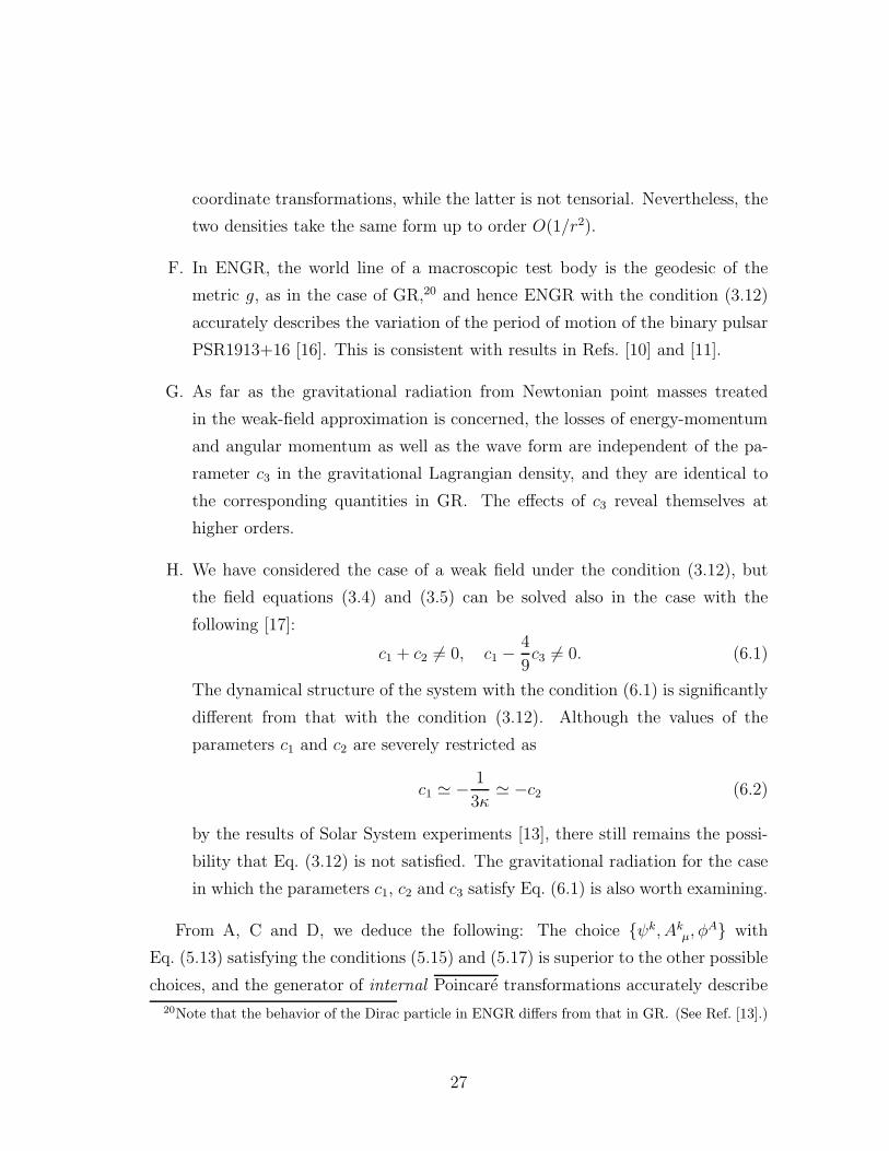
F. In ENGR, the world line of a macroscopic test body is the geodesic of the
metric g, as in the case of GR,20 and hence ENGR with the condition (3.12)
accurately describes the variation of the period of motion of the binary pulsar
PSR1913+16 [16]. This is consistent with results in Refs. [10] and [11].
G. As far as the gravitational radiation from Newtonian point masses treated
in the weak-field approximation is concerned, the losses of energy-momentum
and angular momentum as well as the wave form are independent of the pa-
rameter c3 in the gravitational Lagrangian density, and they are identical to
the corresponding quantities in GR. The effects of c3 reveal themselves at
higher orders.
H. We have considered the case of a weak field under the condition (3.12), but
the field equations (3.4) and (3.5) can be solved also in the case with the
following [17]:
c1 + c2 6= 0, c1 −4
9c3 6= 0. (6.1)
The dynamical structure of the system with the condition (6.1) is significantly
different from that with the condition (3.12). Although the values of the
parameters c1 and c2 are severely restricted as
c1 ≃ − 1
3κ≃ −c2 (6.2)
by the results of Solar System experiments [13], there still remains the possi-
bility that Eq. (3.12) is not satisfied. The gravitational radiation for the case
in which the parameters c1, c2 and c3 satisfy Eq. (6.1) is also worth examining.
From A, C and D, we deduce the following: The choice ψk, Akµ, φ
A with
Eq. (5.13) satisfying the conditions (5.15) and (5.17) is superior to the other possible
choices, and the generator of internal Poincare transformations accurately describe
20Note that the behavior of the Dirac particle in ENGR differs from that in GR. (See Ref. [13].)
27

the energy-momentum and angular momentum for a wide class of gravitating sys-
tems, including space-times in which there are gravitational waves.
In the teleparallel theory of gravity, there have been several attempts [18, 19,
20, 21, 22, 23] to define well-behaved energy-momentum and angular momentum
densities. For the case of the teleparallel equivalent of general relativity, i.e. the case
with the condition (2.27) in our notation, this problem is studied in Refs. [18, 19, 20].
The gravitational energy-momentum density hj ρa in Ref. [18] is the same as our
GTµ
k . In Refs. [19] and [20], Hamiltonian formalism is developed, and a natural
definition of the energy-momentum density of the gravitational field is given. In
addition, the angular-momentum density is examined in Ref. [19]. In Ref. [21], an
energy-momentum current that transforms as a tensor under diffeomorphisms of the
space-time manifold and under global SO(1, 3) transformations is proposed in a co-
frame field formulation of the general teleparallel theory of gravity. In Refs. [22] and
[23], the energy-momentum and angular momentum densities for general teleparallel
theory of an isolated gravitating system are examined.
The energy-momentum and angular momentum for gravitational waves, however,
are not examined in Refs. [18, 19, 20, 21, 22, 23], and in Refs. [19, 20, 21, 22, 23],
the energy-momentum and angular momentum are not related to the generators
of internal Poincare transformations, and there appears no field that corresponds
to our ψk. It is worth examining the relation between their [19, 20, 21, 22, 23]
energy-momentum and angular momentum densities and ours.
Acknowledgements
The authors would like to express their sincere thanks to Professor K. Nakao for
valuable discussions.
A Linearized Einstein Theory
For convenience, we give here a short summary of linearized GR.
28
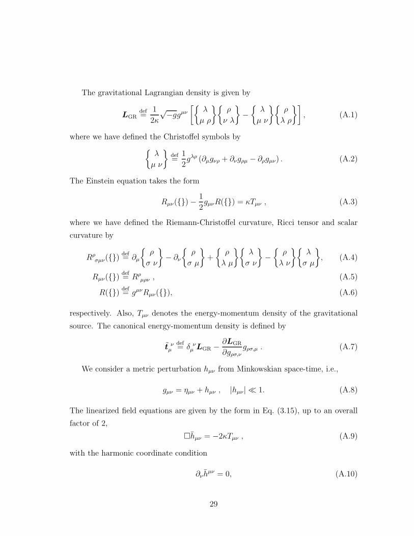
The gravitational Lagrangian density is given by
LGRdef=
1
2κ
√−ggµν
[λ
µ ρ
ρ
ν λ
−
λ
µ ν
ρ
λ ρ
], (A.1)
where we have defined the Christoffel symbols by
λ
µ ν
def=
1
2gλρ (∂µgνρ + ∂νgρµ − ∂ρgµν) . (A.2)
The Einstein equation takes the form
Rµν()−1
2gµνR() = κTµν , (A.3)
where we have defined the Riemann-Christoffel curvature, Ricci tensor and scalar
curvature by
Rρσµν()
def= ∂µ
ρ
σ ν
− ∂ν
ρ
σ µ
+
ρ
λ µ
λ
σ ν
−
ρ
λ ν
λ
σ µ
, (A.4)
Rµν() def= Rρ
µρν , (A.5)
R() def= gµνRµν(), (A.6)
respectively. Also, Tµν denotes the energy-momentum density of the gravitational
source. The canonical energy-momentum density is defined by
t νµ
def= δ ν
µ LGR − ∂LGR
∂gρσ,νgρσ,µ . (A.7)
We consider a metric perturbation hµν from Minkowskian space-time, i.e.,
gµν = ηµν + hµν , |hµν | ≪ 1. (A.8)
The linearized field equations are given by the form in Eq. (3.15), up to an overall
factor of 2,
hµν = −2κTµν , (A.9)
with the harmonic coordinate condition
∂ν hµν = 0, (A.10)
29
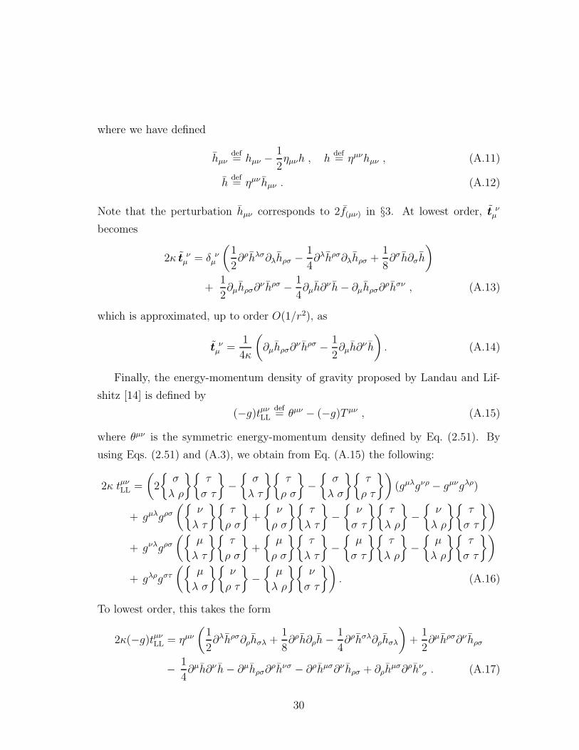
where we have defined
hµνdef= hµν −
1
2ηµνh , h
def= ηµνhµν , (A.11)
hdef= ηµν hµν . (A.12)
Note that the perturbation hµν corresponds to 2f(µν) in §3. At lowest order, t νµ
becomes
2κ t νµ = δ ν
µ
(1
2∂ρhλσ∂λhρσ −
1
4∂λhρσ∂λhρσ +
1
8∂σh∂σh
)
+1
2∂µhρσ∂
ν hρσ − 1
4∂µh∂
ν h− ∂µhρσ∂ρhσν , (A.13)
which is approximated, up to order O(1/r2), as
t νµ =
1
4κ
(∂µhρσ∂
ν hρσ − 1
2∂µh∂
ν h
). (A.14)
Finally, the energy-momentum density of gravity proposed by Landau and Lif-
shitz [14] is defined by
(−g)tµνLLdef= θµν − (−g)T µν , (A.15)
where θµν is the symmetric energy-momentum density defined by Eq. (2.51). By
using Eqs. (2.51) and (A.3), we obtain from Eq. (A.15) the following:
2κ tµνLL =
(2
σ
λ ρ
τ
σ τ
−
σ
λ τ
τ
ρ σ
−
σ
λ σ
τ
ρ τ
)(gµλgνρ − gµνgλρ)
+ gµλgρσ(
ν
λ τ
τ
ρ σ
+
ν
ρ σ
τ
λ τ
−
ν
σ τ
τ
λ ρ
−ν
λ ρ
τ
σ τ
)
+ gνλgρσ(
µ
λ τ
τ
ρ σ
+
µ
ρ σ
τ
λ τ
−µ
σ τ
τ
λ ρ
−
µ
λ ρ
τ
σ τ
)
+ gλρgστ(
µ
λ σ
ν
ρ τ
−
µ
λ ρ
ν
σ τ
). (A.16)
To lowest order, this takes the form
2κ(−g)tµνLL = ηµν(1
2∂λhρσ∂ρhσλ +
1
8∂ρh∂ρh− 1
4∂ρhσλ∂ρhσλ
)+
1
2∂µhρσ∂ν hρσ
− 1
4∂µh∂ν h− ∂µhρσ∂
ρhνσ − ∂ρhµσ∂ν hρσ + ∂ρhµσ∂ρhνσ . (A.17)
30

B Angular Momentum Loss Derived from
Energy-Momentum Loss
Following the argument given in problem 3 in Section 110 of Ref. [14], we derive
the time average of the orbital angular momentum loss for Newtonian point masses
from the time average of the dynamical energy loss given by Eq. (5.5). The result
supports the discussion of the “spin” angular momentum loss given in §5.1.2.We represent the time average of the energy loss of the system as the work of
the “frictional forces” acting on the Newtonian point masses:
⟨dE
dt
⟩=
N∑
a=1
⟨a · ξa
⟩. (B.1)
The time average of the loss of angular momentum, ldef=
∑N
a=1 ξa ×maξa, is given
by ⟨dlαdt
⟩=
N∑
a=1
〈(ξa × a)α〉 =N∑
a=1
ǫαβγ⟨ξβa
γa
⟩, (B.2)
where the symbol ǫαβγ denotes the three-dimensional antisymmetric tensor with
ǫ123 = ǫ123 = 1. Note that a Newtonian point mass in ENGR is subject to Newton’s
equation of motion. To determine a, we write Eq. (5.5) as
⟨dE
dt
⟩= − G
5c5
⟨...Dαβ
...Dαβ −
1
3
...Dαα
...Dββ
⟩= − G
5c5
⟨DαβD
(v)αβ − 1
3DααD
(v)ββ
⟩, (B.3)
where we have used the fact that the average values of the total time derivatives
vanish. Here, D(v)αβ represents the fifth-order derivative with respect to t. Substitut-
ing Dαβ =∑N
a=1ma(ξαa ξ
βa + ξαa ξ
βa ) into Eq. (B.3) and comparing with Eq. (B.1), we
find
αa = −2G
5c5
(D
(v)αβ − 1
3δαβD(v)
γγ
)maξ
βa . (B.4)
Substitution of Eq. (B.4) into Eq. (B.2) gives the result
⟨dlαdt
⟩= −2G
5c5ǫαβγ
⟨(D
(v)γδ − 1
3δγδD(v)
ǫǫ
)Dβδ
⟩= −2G
5c5ǫαβγ
⟨Dβδ
...Dδγ
⟩. (B.5)
This is equivalent to Eq. (5.16), with Eq. (5.13) satisfying the condition (5.17).
31

References
[1] C. W. Misner, K. S. Thorne, and J. A. Wheeler, GRAVITATION (Freeman,
New York, 1973).
[2] R. Geroch and J. Winicour, J. Math. Phys. 22 (1981), 803.
[3] F. W. Hehl, J. D. McCrea, E. W. Mielke and Y. Ne’eman, Phys. Rep. 258
(1995), 1.
[4] T. Kawai, Gen. Relat. Gravit. 18 (1986), 995 [Errata; 19 (1987), 1285].
[5] T. Kawai and N. Toma, Prog. Theor. Phys. 85 (1991), 901.
[6] T. Kawai, Phys. Rev. D 62 (2000), 104014.
[7] T. Kawai, Prog. Theor. Phys. 79 (1988), 920.
[8] T. Kawai and H. Saitoh, Prog. Theor. Phys. 81 (1989), 280.
[9] T. Kawai and H. Saitoh, Prog. Theor. Phys. 81 (1989), 1119.
[10] M. Schweizer and N. Straumann, Phys. Lett. A 71 (1979), 493.
[11] M. Schweizer, N. Straumann and A. Wipf, Gen. Relat. Gravit. 12 (1980), 951.
[12] T. Kawai, Prog. Theor. Phys. 82 (1989), 850.
[13] K. Hayashi and T. Shirafuji, Phys. Rev. D19 (1979), 3524.
[14] L. D. Landau and E. M. Lifshitz, The Classical Theory of Fields (Pergamon
Press, Oxford, 1975).
[15] S. Weinberg, GRAVITATION AND COSMOLOGY: PRINCIPLES AND AP-
PLICATIONS OF THE GENERAL THEORY OF RELATIVITY (John Wiley
& Sons, New York, 1972).
[16] R. A. Hulse and J. H. Taylor, Astrophys. J. 195 (1975), L51.
[17] T. Shirafuji and G. G. L. Nashed, Prog. Theor. Phys. 98 (1997), 1355.
32
[18] V. C. de Andrade, L. C. T. Guillen and J. G. Pereira, Phys. Rev. Lett. 84
(2000), 4533.
[19] J. W. Maluf, J. F. da Rocha-Neto, T. M. L. Torıbio and K. H. Castello Branco,
gr-qc/0008073.
[20] J. W. Maluf and J. F. da Rocha-Neto, Phys. Rev. D 64 (2001), 084014.
[21] Y. Itin, gr-qc/0103017.
[22] M. Blagojevic and M. Vasilic, Class. Quantum Grav. 17 (2000), 3785.
[23] M. Blagojevic and M. Vasilic, Phys. Rev. D 64 (2001), 044010.
33