Embed Size (px)
Citation preview
Energy markets and the implications of renewables
South Australian case study
26 November 2015
© 2015 Deloitte Access Economics Pty Ltd
2
Contents
1 Overview 3
2 Renewable energy in South Australia 7
3 The squeezing out of gas and baseload coal 8
4 Historical Market analysis 14
5 Increasing complexities from additional renewables 19
6 Additional considerations 25
7 Summary 28
© 2015 Deloitte Access Economics Pty Ltd
3
1 Overview
South Australia – a “living experiment” in electricity grids
South Australia finds itself at the cutting edge of contemporary electricity grids. There are countries and regions that have more renewable energy –from Tasmania to Iceland – but have resources such as hydropower (large-scale) and geothermal that are a close substitute for the thermal plant that dominate much of the world’s electricity supply.
These types of plant, along with nuclear, are collectively described as “dispatchable” – meaning the amount of electricity they can supply at any time is subject to the control of the plant’s operator. Nuclear and coal are somewhat less flexible while gas and hydro are more flexible. Plant of any type is subject to the occasional unexpected outage, but electricity systems are set up so that whether via price signals in a market, or simply by direction, other dispatchable plant can ramp up its output or switch on to fill the gap.
South Australia’s renewable resources are in the form of wind and the sun. These resources are described as “intermittent” – they are only available when the wind is blowing or the sun is shining.
There are other regions that have more intermittent renewables, like Denmark and Iowa, but they have strong interconnection to neighbouring regions which facilitate the import or export of electricity equivalent to their peak demand. By contrast, South Australia’s interconnection with Victoria is equivalent to only about 23 per cent of its peak demand1.
1 Based on 2015 peak demand of 2,900MW and interconnection of 680MW (comprising 460MW of existing capacity from Heywood and 220MW from Murraylink)
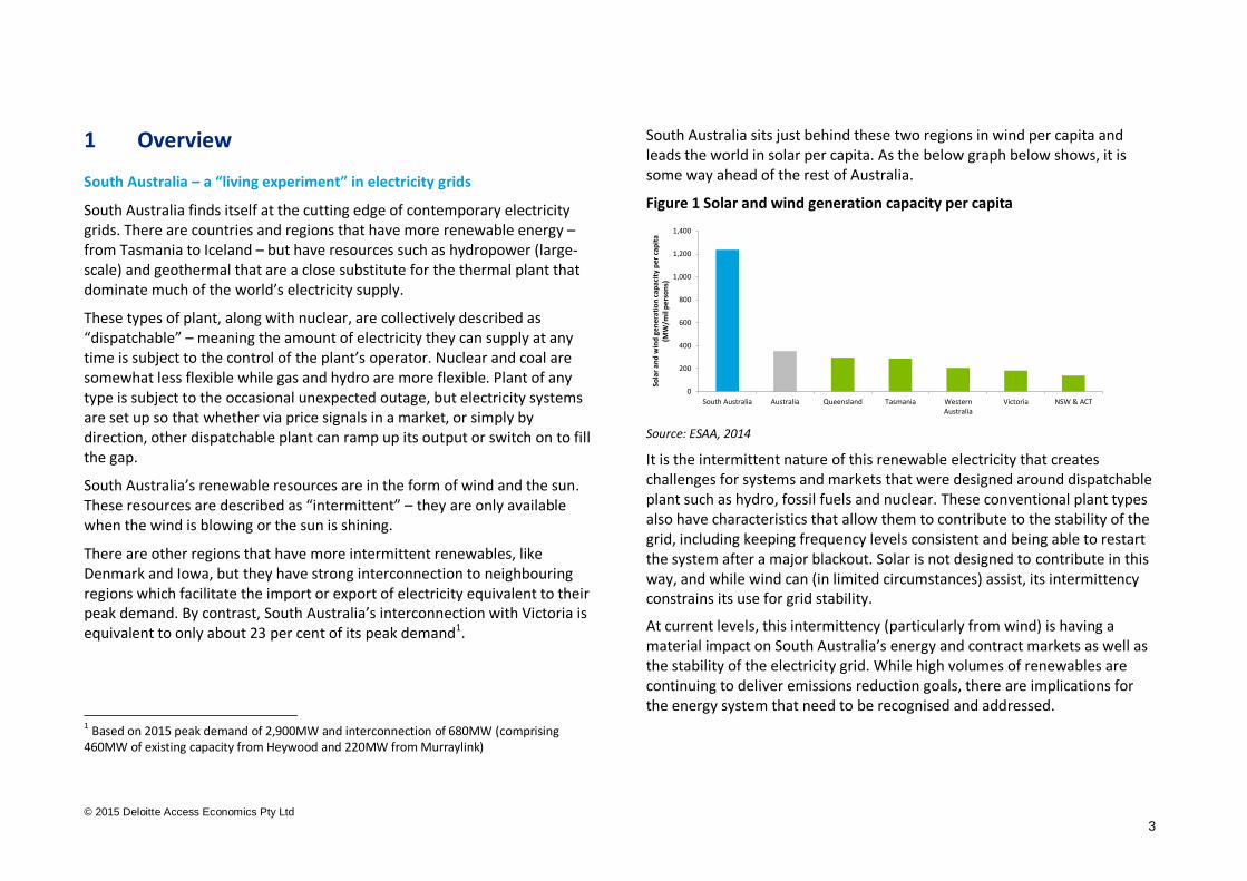
South Australia sits just behind these two regions in wind per capita and leads the world in solar per capita. As the below graph below shows, it is some way ahead of the rest of Australia.
Figure 1 Solar and wind generation capacity per capita
Source: ESAA, 2014
It is the intermittent nature of this renewable electricity that creates challenges for systems and markets that were designed around dispatchable plant such as hydro, fossil fuels and nuclear. These conventional plant types also have characteristics that allow them to contribute to the stability of the grid, including keeping frequency levels consistent and being able to restart the system after a major blackout. Solar is not designed to contribute in this way, and while wind can (in limited circumstances) assist, its intermittency constrains its use for grid stability.
At current levels, this intermittency (particularly from wind) is having a material impact on South Australia’s energy and contract markets as well as the stability of the electricity grid. While high volumes of renewables are continuing to deliver emissions reduction goals, there are implications for the energy system that need to be recognised and addressed.
0
200
400
600
800
1,000
1,200
1,400
South Australia Australia Queensland Tasmania WesternAustralia
Victoria NSW & ACT
Sola
r an
d w
ind
ge
ne
rati
on
cap
acit
y p
er
cap
ita
(MW
/mil
pe
rso
ns)
© 2015 Deloitte Access Economics Pty Ltd
4
In this report, commissioned by the Energy Supply Association of Australia, we investigate the impact that existing levels of renewables are having on the market and the unintended consequences for grid stability that are starting to emerge.
Using South Australia as a case study, we also begin the important discussion on how to address these challenges as wind and solar become the dominant forms of new generation capacity.
Deteriorating returns for dispatchable generation in SA
South Australia is part of the National Energy Market (NEM) that physically covers the east coast of Australia from Port Lincoln on the west coast of South Australia to Port Douglas in north Queensland. Wind generation is typically dispatched ahead of all other generators in the NEM to meet demand. This is reasonable from a resource point of view as wind’s marginal cost of production is virtually zero. This is also the default case with most solar PV, as it is deployed almost exclusively on customers’ rooftops and generates automatically during daylight hours. With flat demand and increasing penetration of wind generation and rooftop PV in SA, the market share for coal and gas generation has reduced significantly over the past 5 years.
The initial growth in renewable generation appeared beneficial for consumers in South Australia. It reduced greenhouse emissions and suppressed wholesale electricity prices as a result of the excess supply created. Reliability and power quality were not compromised because the dispatchable fossil fuel plant was still available to provide energy and grid stability when required. But some of this thermal plant located in South Australia has subsequently become uneconomic as the cost of repair and refurbishment exceeds the reduced margins from weaker wholesale electricity prices.
The result has been the mothballing and closure of surplus generation capacity in South Australia where fixed costs are not being covered. This includes the closure of two coal power stations at Port Augusta (that have already been partially withdrawn from service in recent years), the mothballing of a gas combined cycle plant at Pelican Point and the planned closure of Torrens Island A gas power station.
These are the four largest power stations in South Australia, and they will all be partially or fully removed from the market by 2017.
The impact of losing the generator mix
As these baseload (less flexible plant such as coal) and mid-merit (more flexible, e.g. gas) generators exit the market, the South Australian system is becoming increasingly reliant on interconnection with Victoria (through Heywood and Murraylink) for stability to compensate for intermittent generation. Our modelling outcomes suggest that, by 2019, on average the interconnector is importing all the Victorian electricity into South Australia it can for almost 23 hours per day.
Further withdrawal of baseload and mid-merit plant is also expected to lead to higher energy prices in South Australia as higher cost peaking plants set the market price more frequently. The thermal generation in South Australia effectively becomes gas based, where generation quantities are determined by plant efficiency and fuel price. Although higher prices may signal re-entry or new entry, the net available capacity remains the same.
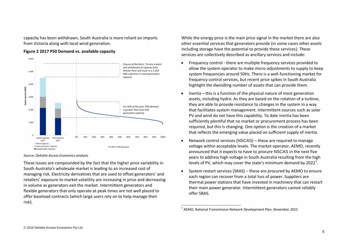
The chart below shows how this available capacity in South Australia may be insufficient to meet demand by 20172. Both supply and demand are calculated on a P50 basis, i.e. the quantity that is expected to be exceeded 50 per cent of the time. Using these median values, it is clear that after the
2 This demand supply balance is projected to largely continue to 2023, until which time new CCGT capacity is brought online
© 2015 Deloitte Access Economics Pty Ltd
5
capacity has been withdrawn, South Australia is more reliant on imports from Victoria along with local wind generation.
Figure 2 2017 P50 Demand vs. available capacity
Source: Deloitte Access Economics analysis
These issues are compounded by the fact that the higher price variability in South Australia’s wholesale market is leading to an increased cost of managing risk. Electricity derivatives that are used to offset generators’ and retailers’ exposure to market volatility are increasing in price and decreasing in volume as generators exit the market. Intermittent generators and flexible generators that only operate at peak times are not well placed to offer baseload contracts (which large users rely on to help manage their risk).
While the energy price is the main price signal in the market there are also other essential services that generators provide (in some cases other assets including storage have the potential to provide these services). These services are collectively described as ancillary services and include:
Frequency control - there are multiple frequency services provided to allow the system operator to make micro-adjustments to supply to keep system frequencies around 50Hz. There is a well-functioning market for frequency control services, but recent price spikes in South Australia highlight the dwindling number of assets that can provide them.
Inertia – this is a function of the physical nature of most generation assets, including hydro. As they are based on the rotation of a turbine, they are able to provide resistance to changes in the system in a way that facilitates system management. Intermittent sources such as solar PV and wind do not have this capability. To date inertia has been sufficiently plentiful that no market or procurement process has been required, but this is changing. One option is the creation of a market that reflects the emerging value placed on sufficient supply of inertia.
Network control services (NSCAS) – these are required to manage voltage within acceptable levels. The market operator, AEMO, recently announced that it expects to have to procure NSCAS in the next five years to address high voltage in South Australia resulting from the high levels of PV, which may cover the state’s minimum demand by 20223.
System restart services (SRAS) – these are procured by AEMO to ensure each region can recover from a total loss of power. Suppliers are thermal power stations that have invested in machinery that can restart their main power generator. Intermittent generators cannot reliably offer SRAS.
3 AEMO, National Transmission Network Development Plan, November 2015
0% 10% 20% 30% 40% 50% 60% 70% 80% 90% 100%
2017 P50 Demand
0
1,000
2,000
3,000
4,000
5,000
6,000
Rated capacity2017
P50 Capacity2017
Rat
ed c
apac
ity
(MW
)
Wind Capacity
Interconnector Capacity
Dispatchable Capacity
Closure of Northern, Torrens A plant and withdrawal of capacity from Pelican Point will result in a 1,250 MW reduction in rated generation capacity
For 50% of the year, P50 demand is greater than local P50 generation capacity
© 2015 Deloitte Access Economics Pty Ltd
6
Where ancillary services are paid for, their costs are recovered from customers and generators. In general, ancillary services can be provided inter-regionally. For example, SA can in principle be supplied from Victoria, but as with energy supply, this is predicated on the reliability and the capacity of interconnection. The changing mix of SA’s electricity supply is likely to both increase demand for and reduce supply of these services.
The future of the energy system
Further intermittent renewable investment (distributed or utility-scale) is likely under a range of potential abatement and other policies. As such, higher prices are expected (relative to other states) as the market price will be set by higher cost generation. While there are options for managing system stability and limiting further exit of baseload and mid-merit generation, there is no clear approach to addressing the challenges posed by an increased share of renewable generation:
Although upgrading the interconnector will alleviate some pressure, increases in capacity can be costly, and South Australia’s risk of wide-scale black out will remain tied to continued interconnection via Heywood and Murraylink.
Flexible demand response has the potential to be a cost-effective approach in the future. But it may take some time to create the products and services that could induce customers to provide demand response on the required scale
Modelling suggests that market signals do not support an increase in flexible thermal generation (above 2017 levels), which may in part be a consequence of intermittent plant receiving a large proportion of their revenue outside the market
Storage could provide a solution that overcomes some of the challenges to the intermittency of wind and solar, but the required deployment at scale is yet to be tested
Given the novel challenges posed by the fundamental changes to the resources in our generation mix, further analysis of the risks to system costs and system stability and the costs and benefits of alternative remedies are required.

© 2015 Deloitte Access Economics Pty Ltd
7
2 Renewable energy in South Australia
2.1 South Australia’s energy mix
Across the world, the proportion of energy generated from renewable sources has been increasing as governments introduce policies to reduce the emissions intensity of the electricity sector, coupled with the improving economics of newer forms of renewable generation such as wind and solar power. Australia is no different, where a number of state and Federal government policies have encouraged renewable generation.
Investment has flowed to those regions where the economics are most attractive, namely those with the best combination of renewable resources, market price signals and government incentives. As a result of solar feed-in tariffs, the large and small scale renewable energy target and some of the best wind resources in Australia, significant investments in solar and wind generation have been made in South Australia. South Australia now has the highest intermittent renewable generation capacity per capita of all States (Figure 3).
Figure 3 Solar and wind generation capacity per capita
Source: ESAA, 2014
Renewable generation capacity as a percentage of total generation capacity in South Australia has increased from 17.5% in FY10 to 38.3% in FY14 (including rooftop PV), an increase of over 100% in just four years (Figure 4).
Figure 4 South Australia's generation mix over time
Source: AEMO South Australian Fuel and Technology Report, 2015
This high penetration of renewable energy has led to significant carbon abatement but there are challenges associated with this energy transition caused by the intermittency of wind and solar generation.
This report explores these challenges by first looking at how forcing renewables into a market can lead to oversupply and the subsequent exiting of baseload coal and mid-merit gas generators that have traditionally supplied a range of services to the grid over and above energy supply. It then examines why this is an important issue for the energy system and grid stability, particularly as more renewables are built.
We also present an analysis of recent history to highlight some of the market responses to the challenge of intermittency of renewables, as well as projecting forward to understand how these challenges might play out under different renewable penetration scenarios.
0
200
400
600
800
1,000
1,200
1,400
South Australia Australia Queensland Tasmania WesternAustralia
Victoria NSW & ACT
Sola
r an
d w
ind
ge
ne
rati
on
cap
acit
y p
er
cap
ita
(MW
/mil
pe
rso
ns)
0%
10%
20%
30%
40%
50%
60%
70%
80%
90%
100%
FY10 FY11 FY12 FY13 FY14
% G
en
ear
tio
n
Natural Gas Other Coal Wind Solar
© 2015 Deloitte Access Economics Pty Ltd
8
3 The squeezing out of gas and baseload coal
In this section, we look at the market dynamics that are leading to the mothballing and closure of coal and gas plant. Out-of-market incentives for renewable generation have flowed primarily to intermittent sources such as wind and solar, especially in South Australia, which lacks hydro resources. These have the particular feature that they are higher cost overall than existing plant (due to their capital costs) but low (effectively zero) short run cost, which means they can displace other forms of generation from dispatch. As intermittent sources, they can only do this periodically, rather than continuously, which means that much of the thermal plant is still required in order that demand can be met.
If the new renewable generators were reliant on energy market revenue to cover their cost, this would act as a natural balancing mechanism to slow down the rate of investment as new plant would find it progressively harder to cover its cost (although rooftop PV is benchmarked more against the retail price, which is much higher than the wholesale price). This would leave sufficient revenue for thermal plant to keep them in the market to the extent necessary to ensure reliable supply.
The consequent effect is squeezing out dispatchable thermal combined cycle gas turbines (CCGT) and baseload coal generation, which as we will see later, play an important part in maintaining stability in a system with high renewable penetration.
3.1 Renewables and the merit order effect
Australia’s National Electricity Market (NEM) connects the Eastern states of Queensland, NSW, Victoria, South Australia and Tasmania. The National Electricity Rules (NER) that govern the NEM are set by the Australian Energy Market Commission (AEMC) and are enforced by the Australian Energy
Regulator (AER). The wholesale electricity market is operated by the Australian Electricity Market Operator (AEMO).
The NEM is an energy only wholesale electricity market. Every five minutes, generators bid generation quantities into the market at prices at which they are willing to be dispatched. AEMO dispatches generators based on the price of bids, with the cheapest generator being dispatched first, until demand is met. The highest or the marginal bid that is dispatched sets the five minute price for each NEM region (each of the five states is a NEM region). AEMO then calculates the half hour spot price (spot price) at each NEM region by averaging the relevant five minute prices. Generators that are dispatched during a half hour receive the spot price for all their generation quantities that are dispatched during that half hour.
As demand changes throughout the day, the market clearing price changes as higher cost generators are called upon to meet higher levels of demand in different regions. This generator ‘merit order’ means that the last generator required to meet market demand (called the marginal generator) sets the market clearing price.
In South Australia, renewables are having a material impact on market outcomes as a result of:
reductions in on-grid demand due to the increased take up of solar PV
an increase in wind generation that has a low marginal cost.
The impact of these forces on the merit order is illustrated in Figure 5. As additional wind generation enters the market, the marginal generator that would have been dispatched and set the marginal price (in the absence of wind generation) is backed-off and not dispatched. Solar has the same effect on the merit order, but does so by reducing demand on the network as solar generation increases throughout the day.
© 2015 Deloitte Access Economics Pty Ltd
9
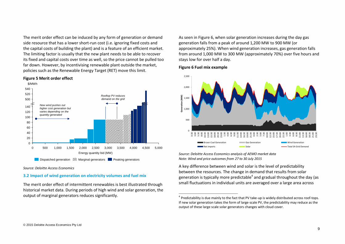
The merit order effect can be induced by any form of generation or demand side resource that has a lower short-run cost (i.e. ignoring fixed costs and the capital costs of building the plant) and is a feature of an efficient market. The limiting factor is usually that the new plant needs to be able to recover its fixed and capital costs over time as well, so the price cannot be pulled too far down. However, by incentivising renewable plant outside the market, policies such as the Renewable Energy Target (RET) move this limit.
Figure 5 Merit order effect
Source: Deloitte Access Economics
3.2 Impact of wind generation on electricity volumes and fuel mix
The merit order effect of intermittent renewables is best illustrated through historical market data. During periods of high wind and solar generation, the output of marginal generators reduces significantly.
As seen in Figure 6, when solar generation increases during the day gas generation falls from a peak of around 1,200 MW to 900 MW (or approximately 25%). When wind generation increases, gas generation falls from around 1,000 MW to 300 MW (approximately 70%) over five hours and stays low for over half a day.
Figure 6 Fuel mix example
Source: Deloitte Access Economics analysis of AEMO market data
Note: Wind and price outcomes from 27 to 30 July 2015
A key difference between wind and solar is the level of predictability between the resources. The change in demand that results from solar generation is typically more predictable4 and gradual throughout the day (as small fluctuations in individual units are averaged over a large area across
4 Predictability is due mainly to the fact that PV take-up is widely distributed across roof-tops. If new solar generation takes the form of large-scale PV, the predictability may reduce as the output of these large scale solar generators changes with cloud cover.
0
Energy quantity bid (MW)
4,5004,0003,5003,0002,5001,500
$/MWh
500
2,000 5,000
20
40
60
80
540
520
140
120
100
5000 1,000
New wind pushes out
higher cost generation but
varies depending on the
quantity generated
Rooftop PV reduces
demand on the grid
Marginal generatorsDispatched generation Peaking generators
0
500
1,000
1,500
2,000
2,500
0:3
0
3:0
0
5:3
0
8:0
0
10
:30
13
:00
15
:30
18
:00
20
:30
23
:00
1:3
0
4:0
0
6:3
0
9:0
0
11
:30
14
:00
16
:30
19
:00
21
:30
0:0
0
2:3
0
5:0
0
7:3
0
10
:00
12
:30
15
:00
17
:30
20
:00
22
:30
1:0
0
3:3
0
6:0
0
8:3
0
11
:00
13
:30
16
:00
18
:30
21
:00
23
:30
Ge
ne
rati
on
(M
W)
Brown Coal Generation Gas Generation Wind Generation
Net imports Solar Total SA Grid Demand
© 2015 Deloitte Access Economics Pty Ltd
10
the state). Wind generation is more localised and therefore has a more visible impact on the market and grid stability e.g. network frequency may vary as a result of large volumes of wind coming online at one time.
In both cases, it is the marginal generators (those in the middle of the merit order), that are most impacted. The volumes of electricity (MWh) they trade in the market are reduced, which has an impact on the economics of the generator. In the case of South Australia, it is the baseload coal and CCGT generators which have been impacted the most, as seen by the recent announced mothballing of Torrens A5, half the capacity of Pelican Point6 and the decision by Alinta to bring forward of the closure of Northern Power Station.
3.3 Impact of wind on spot prices
Given the intermittent nature of wind generation, wind farm operators typically dispatch electricity into the market regardless of price – they currently can’t store energy to sell at a later time for a higher price. The incentive to operate this way is compounded by the fact that they get rewarded outside the market by the RET for every unit of electricity they produce and many wind farms have signed power purchase agreements (PPAs) that pass the risk of low prices to the purchaser (usually a retailer). This means that they are not in a position to ramp up, nor are they incentivised to ramp down production, though technically they could be operated in ways that allow them to do both. Their low marginal cost means they can bid low to clear the market, lowering spot prices through the merit order effect. This means that the large volumes of wind generation in the market not only decreases volumes, but also decreases prices received for baseload and mid-merit plant. 5 https://www.agl.com.au/about-agl/media-centre/article-list/2014/december/agl-to-mothball-south-australian-generating-units 6 http://www.adelaidenow.com.au/news/south-australia/pelican-point-power-station-will-cut-more-than-half-its-generation-capacity-early-next-year-threatening-jobs
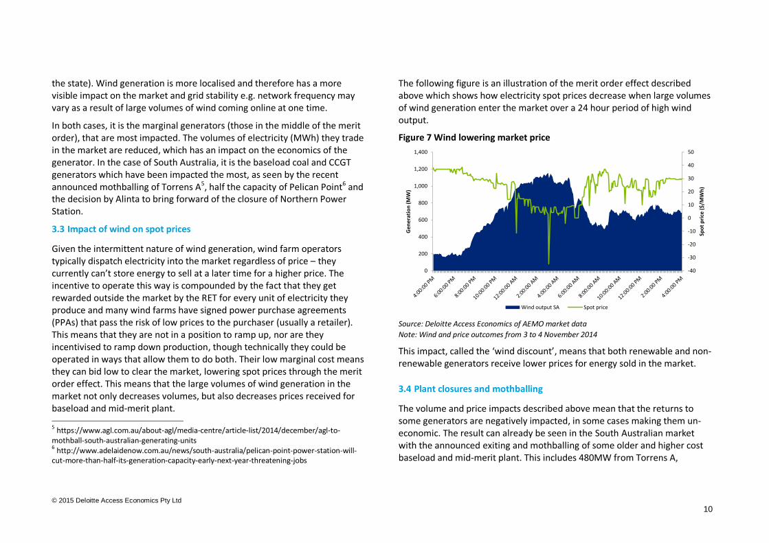
The following figure is an illustration of the merit order effect described above which shows how electricity spot prices decrease when large volumes of wind generation enter the market over a 24 hour period of high wind output.
Figure 7 Wind lowering market price
Source: Deloitte Access Economics of AEMO market data
Note: Wind and price outcomes from 3 to 4 November 2014
This impact, called the ‘wind discount’, means that both renewable and non-renewable generators receive lower prices for energy sold in the market.
3.4 Plant closures and mothballing
The volume and price impacts described above mean that the returns to some generators are negatively impacted, in some cases making them un-economic. The result can already be seen in the South Australian market with the announced exiting and mothballing of some older and higher cost baseload and mid-merit plant. This includes 480MW from Torrens A,
-40
-30
-20
-10
0
10
20
30
40
50
0
200
400
600
800
1,000
1,200
1,400
Spo
t p
rice
($
/MW
h)
Ge
ne
rati
on
(M
W)
Wind output SA Spot price
© 2015 Deloitte Access Economics Pty Ltd
11
530MW from Northern Power Station and a 240MW reduction of capacity at Pelican Point. It can be argued that this is the point of the Renewable Energy Target (RET) – after all it can only reduce emissions by displacing fossil fuel generation. The issue is not that it reduces fossil fuel generation, but whether it does so in a way that may jeopardise reliability and security of supply.
Importantly, these plants are not the most expensive plants in the merit order, and so their eventual withdrawal shifts the merit order back to the right. Other things being equal, the average price increases.
Current generation mix
South Australia’s existing installed capacity is approximately 3,400MW which includes both renewable and non-renewable generation. This generation seems ample to cater for the State’s peak demand of 2,900MW7 but installed capacity is misleading. The rated capacity is rarely (if ever) the quantity of generation that is available at any given time.
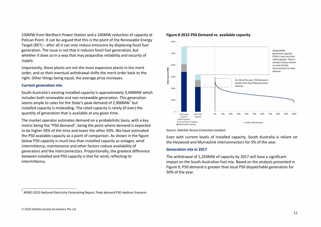
The market operator estimates demand on a probabilistic basis, with a key metric being the “P50 demand”, being the point where demand is expected to be higher 50% of the time and lower the other 50%. We have estimated the P50 available capacity as a point of comparison. As shown in the figure below P50 capacity is much less than installed capacity as outages, wind intermittency, maintenance and other factors reduce availability of generators and the interconnectors. Proportionally, the greatest difference between installed and P50 capacity is that for wind, reflecting its intermittency.
7 AEMO 2015 National Electricity Forecasting Report, Peak demand P50 medium Scenario
Figure 8 2015 P50 Demand vs. available capacity
Source: Deloitte Access Economics analysis
Even with current levels of installed capacity, South Australia is reliant on the Heywood and Murraylink interconnectors for 5% of the year.
Generation mix in 2017
The withdrawal of 1,250MW of capacity by 2017 will have a significant impact on the South Australian fuel mix. Based on the analysis presented in Figure 9, P50 demand is greater than local P50 dispatchable generation for 50% of the year.
0% 10% 20% 30% 40% 50% 60% 70% 80% 90% 100%
2015 P50 Demand
0
1,000
2,000
3,000
4,000
5,000
6,000
2015 ratedcapacity
2015 P50capacity
Rat
ed c
apac
ity
(MW
)
Wind Capacity
Interconnector Capacity
Dispatchable Capacity
Dispatchable generation capacity(P50) is much less than rated capacity. There is already a heavy reliance on wind and the interconnector to meet demand
For 5% of the year, P50 demand is greater than local P50 generation capacity
© 2015 Deloitte Access Economics Pty Ltd
12
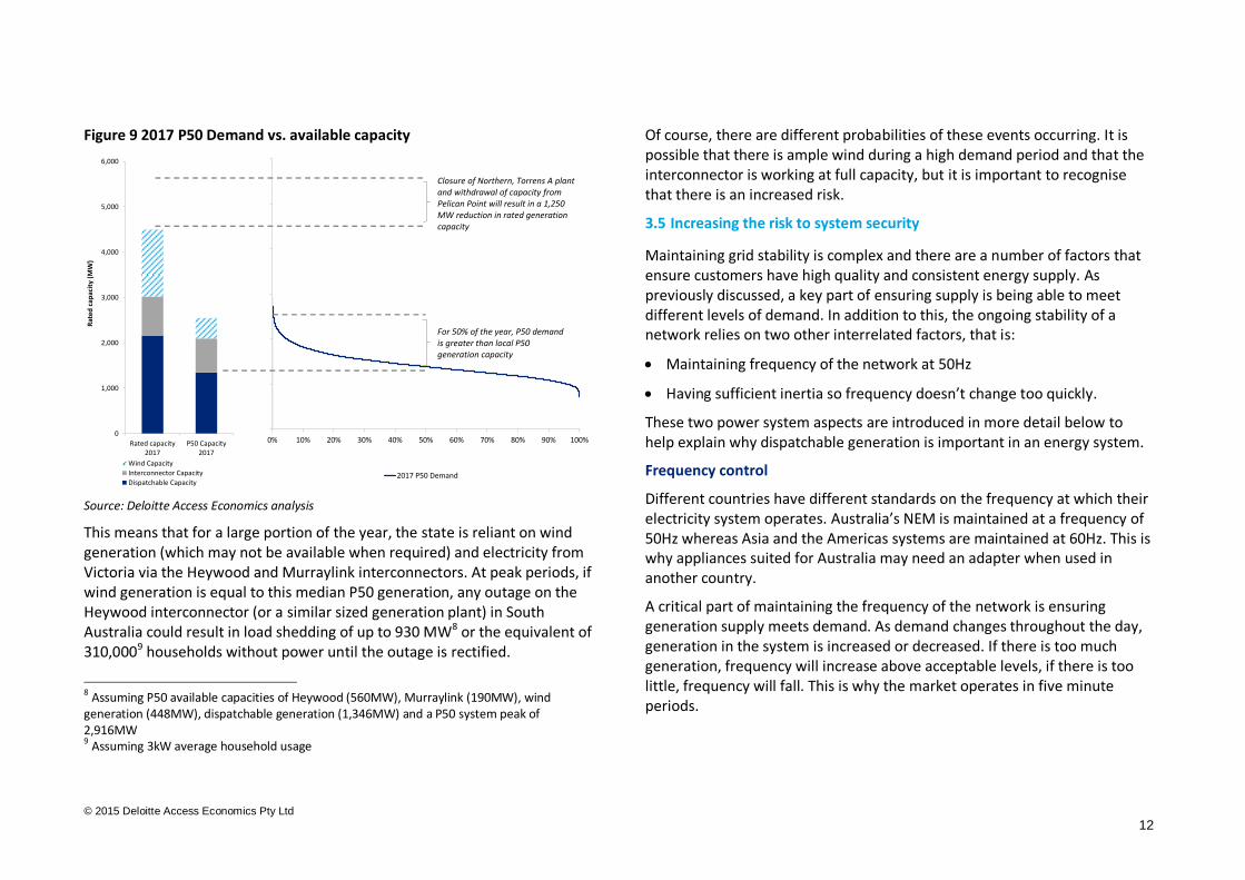
Figure 9 2017 P50 Demand vs. available capacity
Source: Deloitte Access Economics analysis
This means that for a large portion of the year, the state is reliant on wind generation (which may not be available when required) and electricity from Victoria via the Heywood and Murraylink interconnectors. At peak periods, if wind generation is equal to this median P50 generation, any outage on the Heywood interconnector (or a similar sized generation plant) in South Australia could result in load shedding of up to 930 MW8 or the equivalent of 310,0009 households without power until the outage is rectified.
8 Assuming P50 available capacities of Heywood (560MW), Murraylink (190MW), wind generation (448MW), dispatchable generation (1,346MW) and a P50 system peak of 2,916MW 9 Assuming 3kW average household usage
Of course, there are different probabilities of these events occurring. It is possible that there is ample wind during a high demand period and that the interconnector is working at full capacity, but it is important to recognise that there is an increased risk.
3.5 Increasing the risk to system security
Maintaining grid stability is complex and there are a number of factors that ensure customers have high quality and consistent energy supply. As previously discussed, a key part of ensuring supply is being able to meet different levels of demand. In addition to this, the ongoing stability of a network relies on two other interrelated factors, that is:
Maintaining frequency of the network at 50Hz
Having sufficient inertia so frequency doesn’t change too quickly.
These two power system aspects are introduced in more detail below to help explain why dispatchable generation is important in an energy system.
Frequency control
Different countries have different standards on the frequency at which their electricity system operates. Australia’s NEM is maintained at a frequency of 50Hz whereas Asia and the Americas systems are maintained at 60Hz. This is why appliances suited for Australia may need an adapter when used in another country.
A critical part of maintaining the frequency of the network is ensuring generation supply meets demand. As demand changes throughout the day, generation in the system is increased or decreased. If there is too much generation, frequency will increase above acceptable levels, if there is too little, frequency will fall. This is why the market operates in five minute periods.
0% 10% 20% 30% 40% 50% 60% 70% 80% 90% 100%
2017 P50 Demand
0
1,000
2,000
3,000
4,000
5,000
6,000
Rated capacity2017
P50 Capacity2017
Rat
ed c
apac
ity
(MW
)
Wind Capacity
Interconnector Capacity
Dispatchable Capacity
Closure of Northern, Torrens A plant and withdrawal of capacity from Pelican Point will result in a 1,250 MW reduction in rated generation capacity
For 50% of the year, P50 demand is greater than local P50 generation capacity
© 2015 Deloitte Access Economics Pty Ltd
13
If there is a sudden change in the supply demand balance, then frequency can change rapidly within the five minute period. To manage this, there are markets in place which allow AEMO to rebalance supply and demand. These Frequency Control Ancillary Services (or FCAS) are provided by market participants in two forms:
Regulation FCAS – generation units that can be controlled automatically by AEMO to manage small imbalances in load and generation within the five minute dispatch interval
Contingency FCAS – generation units bid in raise and lower quantities to manage larger imbalances that occur within the power system (a contingency event)
Theoretically, these services can be provided by any generator on the grid, including those interstate. However, in the event of separation resulting from interconnector outage, they can only be sourced locally. So in the case of South Australia, as dispatchable generators exit the market, the ability to obtain these services locally is becoming increasingly challenging. While intermittent generators could in principle be configured to provide these services when they are available, their intermittency limits their ability to do so. The impact of this on the cost of FCAS will be explored in the next section.
System inertia
In an electrical power system, inertia is a measure of the rotating mass of a generation unit. In a network such as the NEM, multiple generators are connected through the transmission and distribution network and are synchronised – i.e. they have the same rotational speed, or frequency. Collectively, these rotating generators (and motors) are the inertia in the system. Due to their mass, they will physically resist a change in motion.
The rate of rotation of generators on the network determines the frequency of the system. As such, the greater the inertia in the system the less the
network is susceptible to frequency variations due to sudden disturbances. Conversely, lower levels of inertia mean that a system will experience a greater rate of change of frequency and hence frequency volatility.
Like FCAS, the inertia can be provided from any region in the NEM to any other, except in the event of separation due to interconnector outage. To manage risk, each state typically has minimum acceptable levels of inertia so that the probability of a low inertia event coinciding with separation is very low. Historically, inertia has been provided to a network as a by-product of selling energy. As the majority of energy was supplied by generators with large inertia (‘synchronous’ thermal generators), system inertia levels have been sufficiently high in each NEM region that there was no scarcity value for this service and no need to create a market or procurement process to ensure enough was available for system security needs. However, with the increasing penetration of renewables, this is changing.
In South Australia the high penetration of technologies which are non-synchronous, such as wind and solar, which do not provide inertia, have displaced traditional generators and may be creating a situation where local levels of inertia are low. The market operator has identified these issues and conducted modelling that suggests inertia could fall below acceptable levels for 30% of the year by 2020–21 (assuming 4,000 MWs minimum)10.
While AEMO emergency direction powers could be used to direct generators to increase levels of inertia, these powers are of no use if the required capacity is not available because those generators that could provide it have exited the market. Ultimately, the creation of a market or other procurement process that rewards providers of inertia is the only reliable way to ensure sufficient levels of inertia are maintained. In doing so, all potential providers of inertia should be considered – if renewable plant is able to find ways of doing so, it too should be eligible.
10 AEMO Integrating renewable energy – Wind integration studies report, 2013
© 2015 Deloitte Access Economics Pty Ltd
14
4 Historical Market analysis
In the previous section, we looked at how baseload and mid-merit plant is being pushed out of the market and why this change in generation mix can be an issue for electricity network stability. In the following chapter, we will analyse historical market data to show that these challenges are already being seen in the wholesale electricity and FCAS markets.
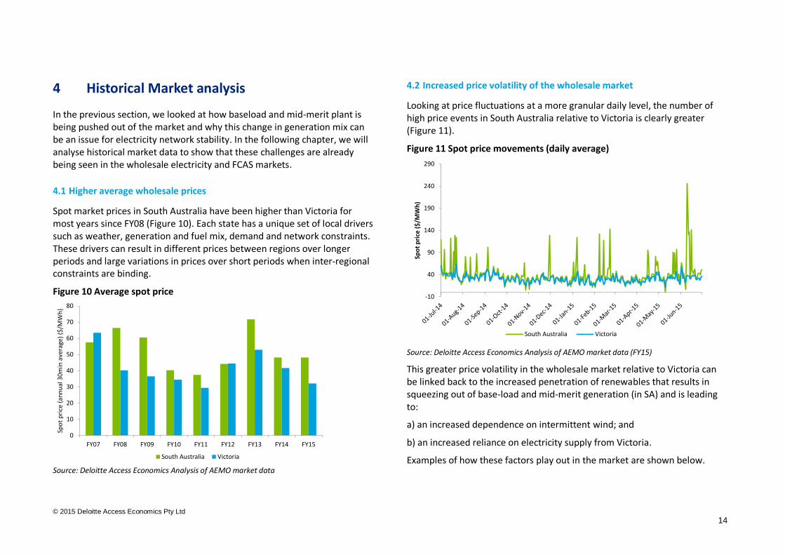
4.1 Higher average wholesale prices
Spot market prices in South Australia have been higher than Victoria for most years since FY08 (Figure 10). Each state has a unique set of local drivers such as weather, generation and fuel mix, demand and network constraints. These drivers can result in different prices between regions over longer periods and large variations in prices over short periods when inter-regional constraints are binding.
Figure 10 Average spot price
Source: Deloitte Access Economics Analysis of AEMO market data
4.2 Increased price volatility of the wholesale market
Looking at price fluctuations at a more granular daily level, the number of high price events in South Australia relative to Victoria is clearly greater (Figure 11).
Figure 11 Spot price movements (daily average)
Source: Deloitte Access Economics Analysis of AEMO market data (FY15)
This greater price volatility in the wholesale market relative to Victoria can be linked back to the increased penetration of renewables that results in squeezing out of base-load and mid-merit generation (in SA) and is leading to:
a) an increased dependence on intermittent wind; and
b) an increased reliance on electricity supply from Victoria.
Examples of how these factors play out in the market are shown below.
0
10
20
30
40
50
60
70
80
FY07 FY08 FY09 FY10 FY11 FY12 FY13 FY14 FY15
Spo
t p
rice
(an
nu
al 3
0m
in a
vera
ge)
($/M
Wh
)
South Australia Victoria
-10
40
90
140
190
240
290
Spo
t p
rice
($
/MW
h)
South Australia Victoria
© 2015 Deloitte Access Economics Pty Ltd
15
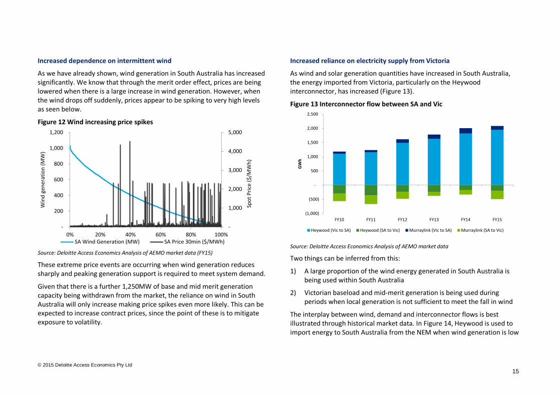
Increased dependence on intermittent wind
As we have already shown, wind generation in South Australia has increased significantly. We know that through the merit order effect, prices are being lowered when there is a large increase in wind generation. However, when the wind drops off suddenly, prices appear to be spiking to very high levels as seen below.
Figure 12 Wind increasing price spikes
Source: Deloitte Access Economics Analysis of AEMO market data (FY15)
These extreme price events are occurring when wind generation reduces sharply and peaking generation support is required to meet system demand.
Given that there is a further 1,250MW of base and mid merit generation capacity being withdrawn from the market, the reliance on wind in South Australia will only increase making price spikes even more likely. This can be expected to increase contract prices, since the point of these is to mitigate exposure to volatility.
Increased reliance on electricity supply from Victoria
As wind and solar generation quantities have increased in South Australia, the energy imported from Victoria, particularly on the Heywood interconnector, has increased (Figure 13).
Figure 13 Interconnector flow between SA and Vic
Source: Deloitte Access Economics Analysis of AEMO market data
Two things can be inferred from this:
1) A large proportion of the wind energy generated in South Australia is being used within South Australia
2) Victorian baseload and mid-merit generation is being used during periods when local generation is not sufficient to meet the fall in wind
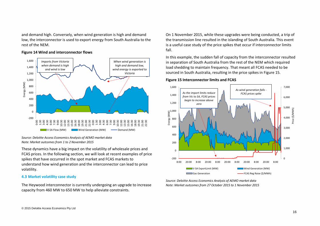
The interplay between wind, demand and interconnector flows is best illustrated through historical market data. In Figure 14, Heywood is used to import energy to South Australia from the NEM when wind generation is low
-
1,000
2,000
3,000
4,000
5,000
-
200
400
600
800
1,000
1,200
0% 20% 40% 60% 80% 100%
Spo
t P
rice
($
/MW
h)
Win
d g
ener
atio
n (
MW
)
SA Wind Generation (MW) SA Price 30min ($/MWh)
(1,000)
(500)
-
500
1,000
1,500
2,000
2,500
FY10 FY11 FY12 FY13 FY14 FY15
GW
h
Heywood (Vic to SA) Heywood (SA to Vic) Murraylink (Vic to SA) Murraylink (SA to Vic)
© 2015 Deloitte Access Economics Pty Ltd
16
and demand high. Conversely, when wind generation is high and demand low, the interconnector is used to export energy from South Australia to the rest of the NEM.
Figure 14 Wind and interconnector flows
Source: Deloitte Access Economics Analysis of AEMO market data
Note: Market outcomes from 1 to 2 November 2015
These dynamics have a big impact on the volatility of wholesale prices and FCAS prices. In the following section, we will look at recent examples of price spikes that have occurred in the spot market and FCAS markets to understand how wind generation and the interconnector can lead to price volatility.
4.3 Market volatility case study
The Heywood interconnector is currently undergoing an upgrade to increase capacity from 460 MW to 650 MW to help alleviate constraints.
On 1 November 2015, while these upgrades were being conducted, a trip of the transmission line resulted in the islanding of South Australia. This event is a useful case study of the price spikes that occur if interconnector limits fall.
In this example, the sudden fall of capacity from the interconnector resulted in separation of South Australia from the rest of the NEM which required load shedding to maintain frequency. That meant all FCAS needed to be sourced in South Australia, resulting in the price spikes in Figure 15.
Figure 15 Interconnector limits and FCAS
Source: Deloitte Access Economics Analysis of AEMO market data
Note: Market outcomes from 27 October 2015 to 1 November 2015
-200
0
200
400
600
800
1,000
1,200
1,400
1,600
0:0
01
:30
3:0
04
:30
6:0
07
:30
9:0
01
0:3
01
2:0
01
3:3
01
5:0
01
6:3
01
8:0
01
9:3
02
1:0
02
2:3
00
:00
1:3
03
:00
4:3
06
:00
7:3
09
:00
10
:30
12
:00
13
:30
15
:00
16
:30
18
:00
19
:30
21
:00
22
:30
Ener
gy (
MW
)
V-SA Flow (MW) Wind Generation (MW) Demand (MW)
When wind generation is high and demand low,
wind energy is exported to Victoria
Imports from Victoria when demand is high
and wind is low
0
1,000
2,000
3,000
4,000
5,000
6,000
7,000
-200
0
200
400
600
800
1,000
1,200
1,400
1,600
8:00 20:00 8:00 20:00 8:00 20:00 8:00 20:00 8:00 20:00 8:00
Pri
ce (
$/M
Wh
)
Ener
gy (
MW
)V-SA ExportLimit (MW) Wind Generation (MW)
Gas Generation FCAS Reg Raise ($/MWh)
As the import limits reducefrom Vic to SA, FCAS prices
begin to increase above zero
As wind generation falls -FCAS prices spike
© 2015 Deloitte Access Economics Pty Ltd
17
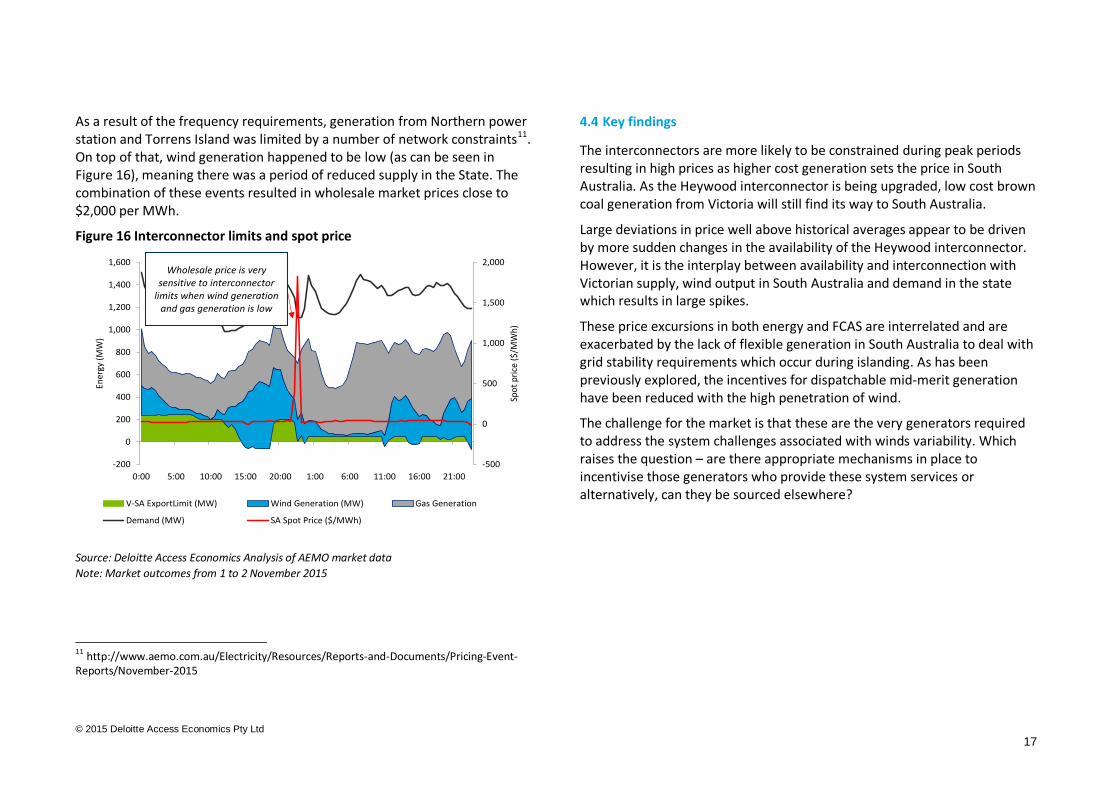
As a result of the frequency requirements, generation from Northern power station and Torrens Island was limited by a number of network constraints11. On top of that, wind generation happened to be low (as can be seen in Figure 16), meaning there was a period of reduced supply in the State. The combination of these events resulted in wholesale market prices close to $2,000 per MWh.
Figure 16 Interconnector limits and spot price
Source: Deloitte Access Economics Analysis of AEMO market data
Note: Market outcomes from 1 to 2 November 2015
11 http://www.aemo.com.au/Electricity/Resources/Reports-and-Documents/Pricing-Event-Reports/November-2015
4.4 Key findings
The interconnectors are more likely to be constrained during peak periods resulting in high prices as higher cost generation sets the price in South Australia. As the Heywood interconnector is being upgraded, low cost brown coal generation from Victoria will still find its way to South Australia.
Large deviations in price well above historical averages appear to be driven by more sudden changes in the availability of the Heywood interconnector. However, it is the interplay between availability and interconnection with Victorian supply, wind output in South Australia and demand in the state which results in large spikes.
These price excursions in both energy and FCAS are interrelated and are exacerbated by the lack of flexible generation in South Australia to deal with grid stability requirements which occur during islanding. As has been previously explored, the incentives for dispatchable mid-merit generation have been reduced with the high penetration of wind.
The challenge for the market is that these are the very generators required to address the system challenges associated with winds variability. Which raises the question – are there appropriate mechanisms in place to incentivise those generators who provide these system services or alternatively, can they be sourced elsewhere?
-500
0
500
1,000
1,500
2,000
-200
0
200
400
600
800
1,000
1,200
1,400
1,600
0:00 5:00 10:00 15:00 20:00 1:00 6:00 11:00 16:00 21:00
Spo
t p
rice
($/
MW
h)
Ener
gy (
MW
)
V-SA ExportLimit (MW) Wind Generation (MW) Gas Generation
Demand (MW) SA Spot Price ($/MWh)
Wholesale price is very sensitive to interconnector
limits when wind generation and gas generation is low
© 2015 Deloitte Access Economics Pty Ltd
18
4.5 Reduces liquidity and higher contract prices
The variability of price in South Australia has implications for electricity derivative markets. The increase in price variability exposes market participants in South Australia to increased levels of risk. Market participants can hedge against wholesale risk by selling or purchasing derivatives such as base swaps or caps.
The suppliers of these derivatives are typically baseload and mid-merit plant who, for example, sell a cap to a retailer. This enables the retailer to ‘cap’ its exposure to high prices in the market to $300/MWh in the case of the NEM. Swaps are used to fix the price for a given volume of energy across the day, which is a useful tool for large industrial users that have consistent demand as well as for retailers. These derivatives also allow generators to increase revenue certainty in a volatile market. Because they are contracts for difference, this only applies to generators that can back the hedges with physical output. If a generator that has sold a derivative is not generating during high prices in the spot market, it will have to pay a lot of money to its counterparty.
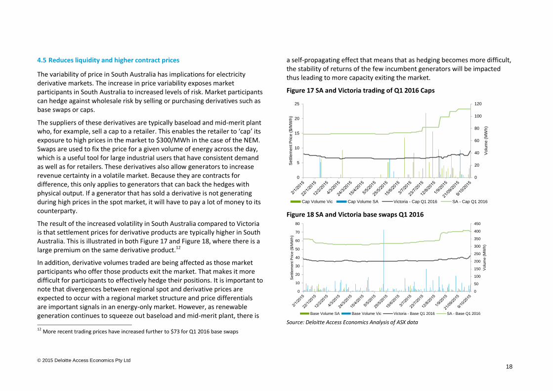
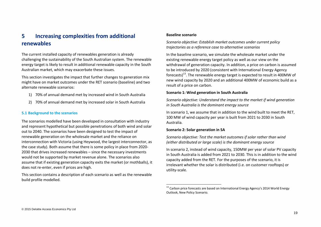
The result of the increased volatility in South Australia compared to Victoria is that settlement prices for derivative products are typically higher in South Australia. This is illustrated in both Figure 17 and Figure 18, where there is a large premium on the same derivative product.12
In addition, derivative volumes traded are being affected as those market participants who offer those products exit the market. That makes it more difficult for participants to effectively hedge their positions. It is important to note that divergences between regional spot and derivative prices are expected to occur with a regional market structure and price differentials are important signals in an energy-only market. However, as renewable generation continues to squeeze out baseload and mid-merit plant, there is 12 More recent trading prices have increased further to $73 for Q1 2016 base swaps
a self-propagating effect that means that as hedging becomes more difficult, the stability of returns of the few incumbent generators will be impacted thus leading to more capacity exiting the market.
Figure 17 SA and Victoria trading of Q1 2016 Caps
Figure 18 SA and Victoria base swaps Q1 2016
Source: Deloitte Access Economics Analysis of ASX data
0
20
40
60
80
100
120
0
5
10
15
20
25
Volu
me (
MW
h)
Sett
lem
ent P
rice (
$/M
Wh)
Cap Volume Vic Cap Volume SA Victoria - Cap Q1 2016 SA - Cap Q1 2016
0
50
100
150
200
250
300
350
400
450
0
10
20
30
40
50
60
70
80
Volu
me (
MW
h)
Sett
lem
ent P
rice (
$/M
Wh)
Base Volume SA Base Volume Vic Victoria - Base Q1 2016 SA - Base Q1 2016
© 2015 Deloitte Access Economics Pty Ltd
19
5 Increasing complexities from additional renewables
The current installed capacity of renewables generation is already challenging the sustainability of the South Australian system. The renewable energy target is likely to result in additional renewable capacity in the South Australian market, which may exacerbate these issues.
This section investigates the impact that further changes to generation mix might have on market outcomes under the RET scenario (baseline) and two alternate renewable scenarios:
1) 70% of annual demand met by increased wind in South Australia
2) 70% of annual demand met by increased solar in South Australia
5.1 Background to the scenarios
The scenarios modelled have been developed in consultation with industry and represent hypothetical but possible penetrations of both wind and solar out to 2040. The scenarios have been designed to test the impact of renewable generation on the wholesale market and the reliance on interconnection with Victoria (using Heywood, the largest interconnector, as the case study). Both assume that there is some policy in place from 2020-2030 that drives increased renewables – since the necessary investments would not be supported by market revenue alone. The scenarios also assume that if existing generation capacity exits the market (or mothballs), it does not re-enter, even if prices are high.
This section contains a description of each scenario as well as the renewable build profile modelled.
Baseline scenario
Scenario objective: Establish market outcomes under current policy trajectories as a reference case to alternative scenarios
In the baseline scenario, we simulate the wholesale market under the existing renewable energy target policy as well as our view on the withdrawal of generation capacity. In addition, a price on carbon is assumed to be introduced by 2020 (consistent with International Energy Agency forecasts)13. The renewable energy target is expected to result in 400MW of new wind capacity by 2020 and an additional 400MW of economic build as a result of a price on carbon.
Scenario 1: Wind generation in South Australia
Scenario objective: Understand the impact to the market if wind generation in South Australia is the dominant energy source
In scenario 1, we assume that in addition to the wind built to meet the RET, 100 MW of wind capacity per year is built from 2021 to 2030 in South Australia.
Scenario 2: Solar generation in SA
Scenario objective: Test the market outcomes if solar rather than wind (either distributed or large scale) is the dominant energy source
In scenario 2, instead of wind capacity, 150MW per year of solar PV capacity in South Australia is added from 2021 to 2030. This is in addition to the wind capacity added from the RET. For the purposes of the scenario, it is irrelevant whether the solar is distributed (i.e. on customer rooftops) or utility-scale.
13 Carbon price forecasts are based on International Energy Agency’s 2014 World Energy Outlook, New Policy Scenario.
© 2015 Deloitte Access Economics Pty Ltd
20
5.2 Model assumptions and generation mix
Deloitte’s Electricity Market Model (DEMM) uses a combination of optimisation and game-theoretic models to simulate the investment, bidding and dispatch behaviour of NEM participants to meet long term growth in electricity demand and emission constraints (using AEMO projects for demand growth). It is a forty block model which enables sufficient granularity to investigate annual trends and inter regional flows, whilst being efficient at conducting scenario analysis.
The model encompasses the following elements:
• Optimisation of generation units considering fuel, operating and carbon costs
• Generator bidding strategies using a transmission constrained Cournot Nash equilibrium model – this simulates generator behaviour in competitive market where trade-offs are made between price and output
• Inter-regional market dynamics given constraints on transmission capacity
• Investment in and retirement of generating units over the planning horizon to meet demand.
In each scenario, the new generation capacity that is added is done so to achieve a higher proportion of annual energy consumption in South Australia that is met by renewable generation.
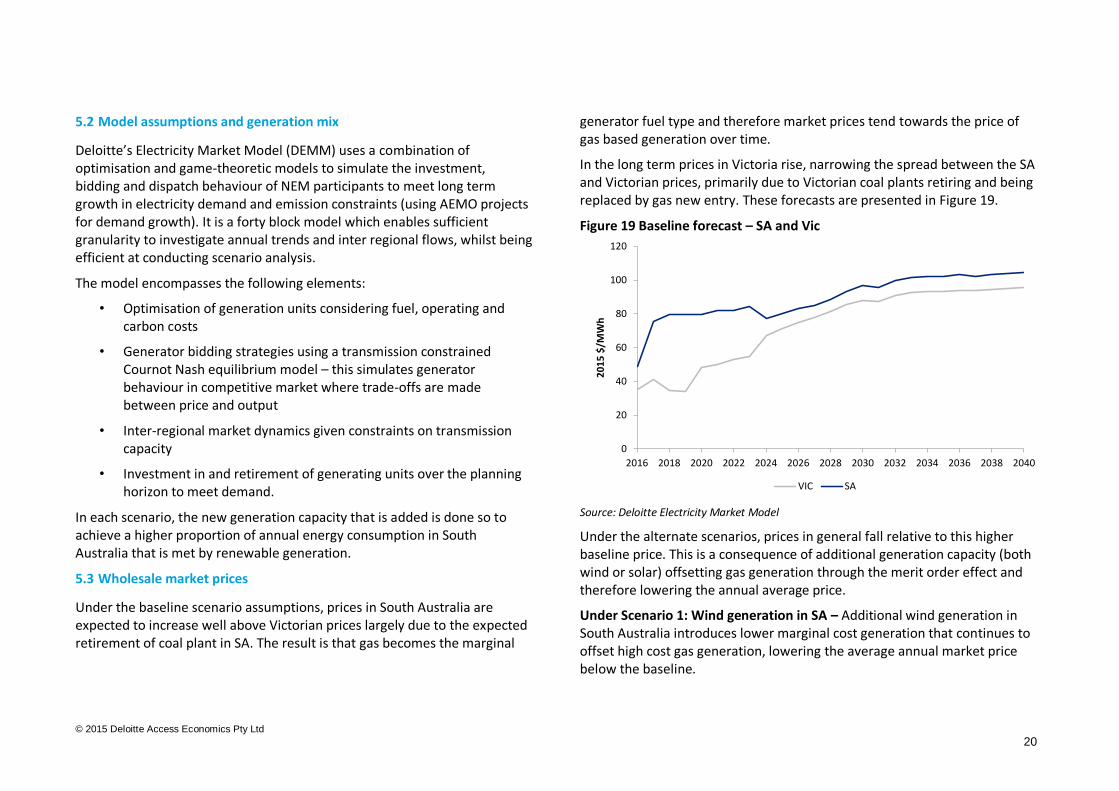
5.3 Wholesale market prices
Under the baseline scenario assumptions, prices in South Australia are expected to increase well above Victorian prices largely due to the expected retirement of coal plant in SA. The result is that gas becomes the marginal
generator fuel type and therefore market prices tend towards the price of gas based generation over time.
In the long term prices in Victoria rise, narrowing the spread between the SA and Victorian prices, primarily due to Victorian coal plants retiring and being replaced by gas new entry. These forecasts are presented in Figure 19.
Figure 19 Baseline forecast – SA and Vic
Source: Deloitte Electricity Market Model
Under the alternate scenarios, prices in general fall relative to this higher baseline price. This is a consequence of additional generation capacity (both wind or solar) offsetting gas generation through the merit order effect and therefore lowering the annual average price.
Under Scenario 1: Wind generation in SA – Additional wind generation in South Australia introduces lower marginal cost generation that continues to offset high cost gas generation, lowering the average annual market price below the baseline.
0
20
40
60
80
100
120
2016 2018 2020 2022 2024 2026 2028 2030 2032 2034 2036 2038 2040
20
15
$/M
Wh
VIC SA
© 2015 Deloitte Access Economics Pty Ltd
21
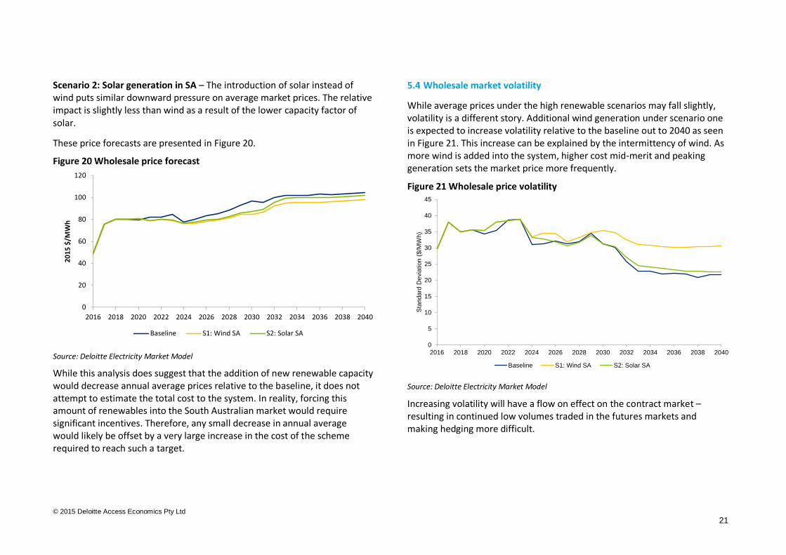
Scenario 2: Solar generation in SA – The introduction of solar instead of wind puts similar downward pressure on average market prices. The relative impact is slightly less than wind as a result of the lower capacity factor of solar.
These price forecasts are presented in Figure 20.
Figure 20 Wholesale price forecast
Source: Deloitte Electricity Market Model
While this analysis does suggest that the addition of new renewable capacity would decrease annual average prices relative to the baseline, it does not attempt to estimate the total cost to the system. In reality, forcing this amount of renewables into the South Australian market would require significant incentives. Therefore, any small decrease in annual average would likely be offset by a very large increase in the cost of the scheme required to reach such a target.
5.4 Wholesale market volatility
While average prices under the high renewable scenarios may fall slightly, volatility is a different story. Additional wind generation under scenario one is expected to increase volatility relative to the baseline out to 2040 as seen in Figure 21. This increase can be explained by the intermittency of wind. As more wind is added into the system, higher cost mid-merit and peaking generation sets the market price more frequently.
Figure 21 Wholesale price volatility
Source: Deloitte Electricity Market Model
Increasing volatility will have a flow on effect on the contract market – resulting in continued low volumes traded in the futures markets and making hedging more difficult.
0
20
40
60
80
100
120
2016 2018 2020 2022 2024 2026 2028 2030 2032 2034 2036 2038 2040
20
15
$/M
Wh
Baseline S1: Wind SA S2: Solar SA
0
5
10
15
20
25
30
35
40
45
2016 2018 2020 2022 2024 2026 2028 2030 2032 2034 2036 2038 2040
Sta
ndard
Devia
tion (
$/M
Wh)
Baseline S1: Wind SA S2: Solar SA
© 2015 Deloitte Access Economics Pty Ltd
22
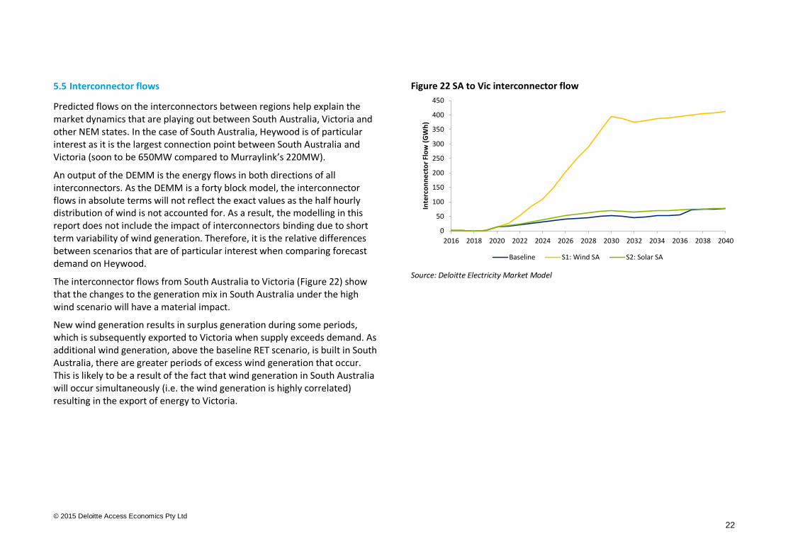
5.5 Interconnector flows
Predicted flows on the interconnectors between regions help explain the market dynamics that are playing out between South Australia, Victoria and other NEM states. In the case of South Australia, Heywood is of particular interest as it is the largest connection point between South Australia and Victoria (soon to be 650MW compared to Murraylink’s 220MW).
An output of the DEMM is the energy flows in both directions of all interconnectors. As the DEMM is a forty block model, the interconnector flows in absolute terms will not reflect the exact values as the half hourly distribution of wind is not accounted for. As a result, the modelling in this report does not include the impact of interconnectors binding due to short term variability of wind generation. Therefore, it is the relative differences between scenarios that are of particular interest when comparing forecast demand on Heywood.
The interconnector flows from South Australia to Victoria (Figure 22) show that the changes to the generation mix in South Australia under the high wind scenario will have a material impact.
New wind generation results in surplus generation during some periods, which is subsequently exported to Victoria when supply exceeds demand. As additional wind generation, above the baseline RET scenario, is built in South Australia, there are greater periods of excess wind generation that occur. This is likely to be a result of the fact that wind generation in South Australia will occur simultaneously (i.e. the wind generation is highly correlated) resulting in the export of energy to Victoria.
Figure 22 SA to Vic interconnector flow
Source: Deloitte Electricity Market Model
0
50
100
150
200
250
300
350
400
450
2016 2018 2020 2022 2024 2026 2028 2030 2032 2034 2036 2038 2040
Inte
rco
nn
ect
or
Flo
w (
GW
h)
Baseline S1: Wind SA S2: Solar SA
© 2015 Deloitte Access Economics Pty Ltd
23
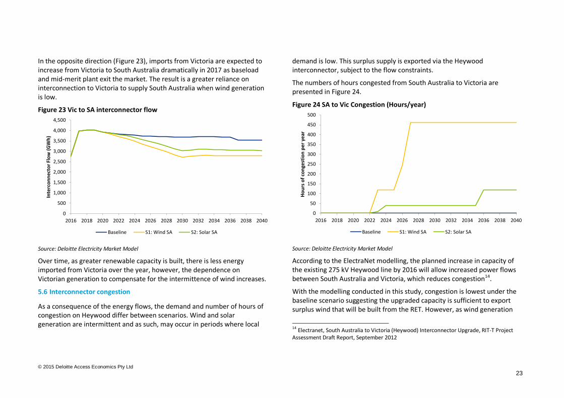
In the opposite direction (Figure 23), imports from Victoria are expected to increase from Victoria to South Australia dramatically in 2017 as baseload and mid-merit plant exit the market. The result is a greater reliance on interconnection to Victoria to supply South Australia when wind generation is low.
Figure 23 Vic to SA interconnector flow
Source: Deloitte Electricity Market Model
Over time, as greater renewable capacity is built, there is less energy imported from Victoria over the year, however, the dependence on Victorian generation to compensate for the intermittence of wind increases.
5.6 Interconnector congestion
As a consequence of the energy flows, the demand and number of hours of congestion on Heywood differ between scenarios. Wind and solar generation are intermittent and as such, may occur in periods where local
demand is low. This surplus supply is exported via the Heywood interconnector, subject to the flow constraints.
The numbers of hours congested from South Australia to Victoria are presented in Figure 24.
Figure 24 SA to Vic Congestion (Hours/year)
Source: Deloitte Electricity Market Model
According to the ElectraNet modelling, the planned increase in capacity of the existing 275 kV Heywood line by 2016 will allow increased power flows between South Australia and Victoria, which reduces congestion14.
With the modelling conducted in this study, congestion is lowest under the baseline scenario suggesting the upgraded capacity is sufficient to export surplus wind that will be built from the RET. However, as wind generation
14 Electranet, South Australia to Victoria (Heywood) Interconnector Upgrade, RIT-T Project Assessment Draft Report, September 2012
0
500
1,000
1,500
2,000
2,500
3,000
3,500
4,000
4,500
2016 2018 2020 2022 2024 2026 2028 2030 2032 2034 2036 2038 2040
Inte
rco
nn
ect
or
Flo
w (
GW
h)
Baseline S1: Wind SA S2: Solar SA
0
50
100
150
200
250
300
350
400
450
500
2016 2018 2020 2022 2024 2026 2028 2030 2032 2034 2036 2038 2040
Ho
urs
of
con
gest
ion
pe
r ye
ar
Baseline S1: Wind SA S2: Solar SA
© 2015 Deloitte Access Economics Pty Ltd
24
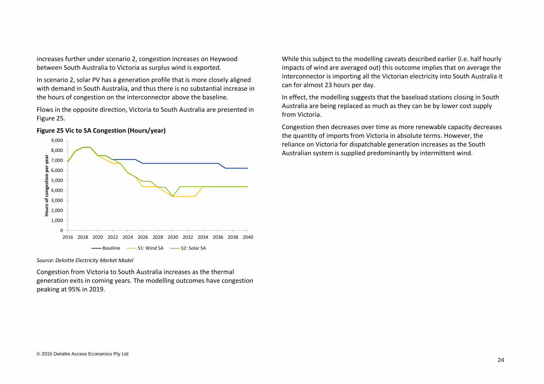
increases further under scenario 2, congestion increases on Heywood between South Australia to Victoria as surplus wind is exported.
In scenario 2, solar PV has a generation profile that is more closely aligned with demand in South Australia, and thus there is no substantial increase in the hours of congestion on the interconnector above the baseline.
Flows in the opposite direction, Victoria to South Australia are presented in Figure 25.
Figure 25 Vic to SA Congestion (Hours/year)
Source: Deloitte Electricity Market Model
Congestion from Victoria to South Australia increases as the thermal generation exits in coming years. The modelling outcomes have congestion peaking at 95% in 2019.
While this subject to the modelling caveats described earlier (i.e. half hourly impacts of wind are averaged out) this outcome implies that on average the interconnector is importing all the Victorian electricity into South Australia it can for almost 23 hours per day.
In effect, the modelling suggests that the baseload stations closing in South Australia are being replaced as much as they can be by lower cost supply from Victoria.
Congestion then decreases over time as more renewable capacity decreases the quantity of imports from Victoria in absolute terms. However, the reliance on Victoria for dispatchable generation increases as the South Australian system is supplied predominantly by intermittent wind.
0
1,000
2,000
3,000
4,000
5,000
6,000
7,000
8,000
9,000
2016 2018 2020 2022 2024 2026 2028 2030 2032 2034 2036 2038 2040
Ho
urs
of
con
gest
ion
pe
r ye
ar
Baseline S1: Wind SA S2: Solar SA
© 2015 Deloitte Access Economics Pty Ltd
25
6 Additional considerations
6.1 The decreasing price signals for wind
While South Australia has some of the best wind resource in Australia, the market dynamics investigated are starting to tell a different story on the case for investment.
The greater the wind generation in the market – the lower average price a wind generator will receive. This means that each new wind generator is creating an environment that actually reduces spot revenue, particularly if that wind farm has output that is correlated to the rest of the market.
Furthermore, the prices that wind farms are likely to receive are inversely correlated to the high price events that occur in the system. Typically, they generate during periods of low demand (in the evening) which is not when higher prices in the market occur.
If the South Australian market were to continue on its current path, then the case for new wind will become less attractive. While a joint study by AEMO and Electranet15 suggests that the increase in capacity to Heywood from July 2016 from 460MW to 650MW will allow additional exports of South Australian wind generation, our scenario modelling in the previous section shows that the constraint is likely to only be alleviated temporarily as wind investment continues.
6.2 Are there increasing price signals for solar?
There has been little in the way of development of grid connected large scale solar systems across the NEM but as costs come down and programs that target large scale solar are rolled out, this is expected to change.
15 AEMO and Electranet (2014) Renewable Energy Integration in Australia , October 2014
Solar has the benefit of being somewhat correlated to periods of higher demand and not correlated to wind. This means, the average price a solar farm can receive from the market has the potential to be greater than wind (on an as generated basis). If capital costs continue to fall and prices rise in South Australia as expected, then it is likely that we will start to see a switch from wind to solar for large scale renewable projects.
The outlook for distributed solar is still positive. The economics of residential (and commercial) solar may become more compelling as the rise in wholesale price flows through to retail tariffs. If capital costs continue to decrease (and the Australian dollar doesn’t fall) then residential solar (with existing feed-in tariffs) is likely to continue its growth.
Growth in both large and small scale solar will still be limited by demand in the state. AEMO has forecast that distributed solar could meet SA’s minimum demand as early as 202216, meaning that the economics of large-scale solar could be limited beyond this point.
6.3 Voltage management
The growing level of solar PV in the system may catalyse the requirement for a new ancillary service. Network control services (NSCAS) are required to manage voltage within acceptable levels. The market operator, AEMO, recently announced that it expects to have to procure NSCAS in the next five years to address high voltage in South Australia resulting from the increasing levels of PV17.
16 AEMO, 2015 National Electricity Forecasting Report 17 AEMO, National Transmission Network Development Plan, November 2015
© 2015 Deloitte Access Economics Pty Ltd
26
6.4 System restart services
To cover the contingency of a widespread blackout, some of the generators on the system need independent facilities that allow them to restart their main generator and return power supply to the system as quickly as possible. To this end, AEMO procures System Restart Ancillary Services. Only dispatchable generation is in a position to do this. Based on power system modelling of the number of restart facilitates required to return the system to power on a timely basis, AEMO currently procures two SRAS services in South Australia18. In principle, then, SRAS could be available with a minimum of two large thermal generators in the region. However, as the number of potential providers decreases, the cost of procuring SRAS is likely to rise.
6.5 Volatility and the impact of storage
Some market participants suggest that storage may provide the answer to some of the challenges faced by the South Australian market. Storage (both large scale and small) allows the purchase of electricity at low prices and which can then be sold when prices are high, effectively taking advantage or price volatility in the market.
In this way storage smooths demand for generated electricity as well as price fluctuations, which means it could be used to improve returns for incumbents (if large scale).
Storage can also be installed at the network and household level. If storage (including network storage) is installed downstream of network constraints, the potential benefits are larger.
The economics of storage are largely driven by:
Capital cost – the upfront cost of installation and commissioning of a storage system
18 AEMO, SRAS Completion Report, July 2015
Electricity price differential—the difference between the market price at which electricity can be bought (and sold) and the peak price that the stored energy will displace.
Electricity price differential frequency—the more often price differentials arise, the more often storage can profitably be used. This spreads the capital cost of storage over more MWh, thus reducing the unit cost of storage and improving its commerciality.
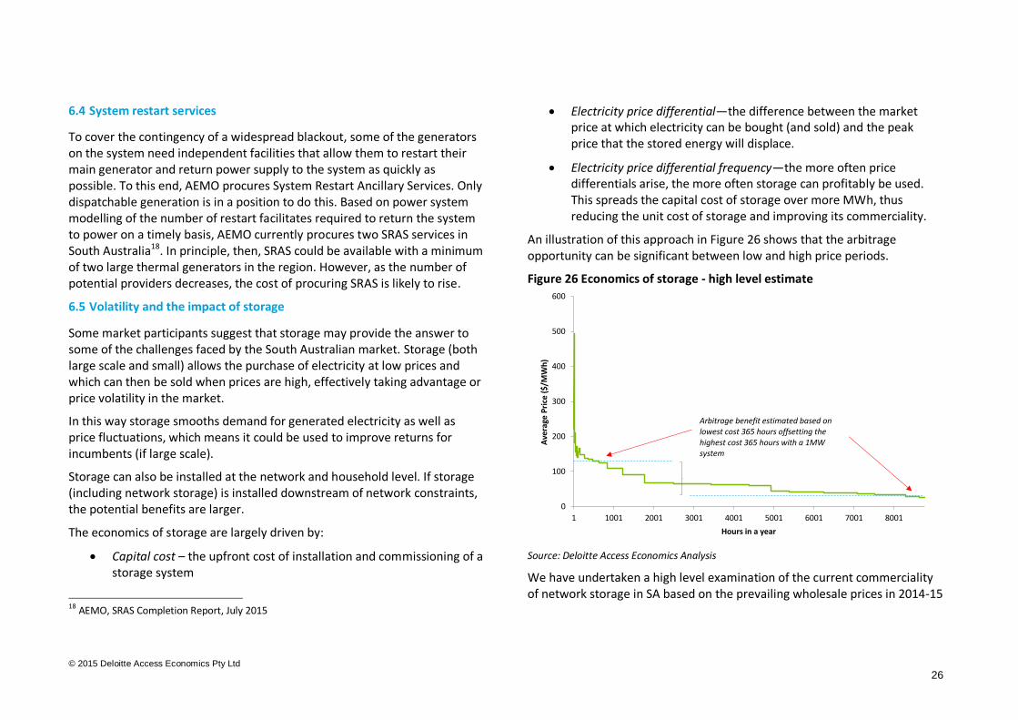
An illustration of this approach in Figure 26 shows that the arbitrage opportunity can be significant between low and high price periods.
Figure 26 Economics of storage - high level estimate
Source: Deloitte Access Economics Analysis
We have undertaken a high level examination of the current commerciality of network storage in SA based on the prevailing wholesale prices in 2014-15
0
100
200
300
400
500
600
1 1001 2001 3001 4001 5001 6001 7001 8001
Ave
rage
Pri
ce (
$/M
Wh
)
Hours in a year
Arbitrage benefit estimated based on lowest cost 365 hours offsetting the highest cost 365 hours with a 1MW system
© 2015 Deloitte Access Economics Pty Ltd
27
and forecast prices to 2025. We have used the following simplifying assumptions:
Storage costs and specifications are based on the Tesla Powerpack (approximately $400,000 AUD for a 1 MWh discharge system) with a 10 year life and a 90% efficiency
Storage can discharge once each day, and the cost of recharging is based on off-peak electricity price (10 year average charge price $27.7/MWh)
Stored electricity is discharged during periods of peak price meaning high price event effectively reduced to lower cost of charging (10 year average charge price $182.3/MWh)
The estimated savings under these assumptions each year over a 10 year period are multiplied by the arbitrage opportunity (182.3 – 27.7) = $154.6 (per MWh of installed storage discharge capacity). Over the course of a year, this equates to $56,400 of savings with a present value of approximately $380,000 for ten years (at 8% discount rate).
Based on these simplified assumptions the price of network storage would only need to fall by around 5% to become theoretically viable. That is, the $400,000 upfront cost to fall to less than $380,000 in today’s dollars.
In reality, storage costs are likely to be higher than modelled because our analysis has not included costs of registration, IT or opex needed to operate a large scale storage facility. Our modelling also assumes that storage operators will discharge at peak times whereas this may not be achievable in all cases, if for example a long period of peak prices occurs.
While the economics of storage may be close to viable under such assumptions, it is important to consider the impact that wide scale uptake of storage can have. As storage penetration increases, the price volatility of the market will decrease as storage units flatten out supply and demand
dynamics. As such, the volatility that made the investment attractive in the first place may no longer exist if sufficient storage is installed.
Taking these factors into account, storage costs are likely to need to fall much further than the simplified example above to be reliably economic investments.
© 2015 Deloitte Access Economics Pty Ltd
28
7 Summary
South Australia’s renewable penetration has increased to the extent that both solar and wind are having a material impact on the market. Rooftop solar is decreasing demand on the grid and wind generation is delivering low cost energy into the market.
Market volatility is increasing as these intermittent technologies increase in penetration and as such, the risk in the market and the cost to hedge against that risk through derivative products is becoming prohibitive.
The combination of these market outcomes is that the incentives for some of the incumbent fossil fuel generators to participate in the market are being reduced in the short run. This would not necessarily be a concern were it not for the stability that these incumbent generators provide to the network.
The consequences of these market dynamics are already being felt with removal of 1250MW of capacity. Although alternative scenarios of higher penetration of wind and solar may lower wholesale prices – providing this does not induce further exit of thermal plant – they would require subsidies and will increase volatility and reliance on the interconnector.
7.1 Options to deal with grid stability
There are a number of options to deal with the issues presented in this report which have been identified by the AEMO, Electranet and industry participants. Such options would require changes to processes, systems and regulatory instruments, such as:
Arrangements to ensure minimum levels of synchronous generation remain online in SA. This could take many forms, including reliability payments or a capacity market. Such arrangements are used or being trialled in other markets in Europe and North America.
Development of new ancillary service markets, such as localised provision of inertia and frequency regulation
Network augmentation options such as high inertia synchronous condensers
Modifications to the controls of the Murraylink interconnector
Changes to the NER to give AEMO greater dispatch powers for non-credible events (which may in itself lead to inefficiencies as market signals are eroded)
Limiting the output of non-synchronous generation.
What is clear is that there are a number of options that need further investigation. It is important that any assessment of these options does not place preference on any one technology or geographical solution as this may result in inefficient market outcomes and ultimately higher costs to the consumer.
7.2 Areas for further investigation
This study focussed on analysing the impact that wind and solar generation are having on the wholesale and derivative markets in SA and the potential impact on grid stability.
Our analysis looked ahead to a potential future where such technologies provide around 70 per cent or more of the state’s generation and considered how robust the market is to these outcomes. However, there are a number of areas that require further investigation that would contribute to the policy discussion. Namely:
Investigating the net market benefits of further interconnection upgrades between Victoria and SA
Estimating the saturation point of both rooftop solar, wind and large scale solar both in isolation and in combination

© 2015 Deloitte Access Economics Pty Ltd
29
Understanding the implications of network constraints outside of South Australia that may be affecting the ability to transport wind energy out of the state
Investigating if there is a case for a market in inertia or other ancillary services not covered by FCAS.
Investigating if there is a case for a market in capacity, noting that this would entail a fundamental change in market design
Investigating the scope for efficient demand response that could allow a portion of demand to follow supply rather than vice versa, noting that this would be a long-term development.
It is important that these investigations are agnostic of technology while recognising the importance of a transition to a lower emissions energy system if Australia is to meet its international emissions reduction commitments. South Australia has a unique opportunity to be a test case for a establishing a reliable, stable high renewable penetration energy system. An economically efficient path to achieving this outcome is beneficial to all.
© 2015 Deloitte Access Economics Pty Ltd
30
About Deloitte
Deloitte refers to one or more of Deloitte Touche Tohmatsu Limited, a UK private company limited by guarantee, and its network of member firms,
each of which is a legally separate and independent entity. Please see www.deloitte.com/au/about for a detailed description of the legal structure of
Deloitte Touche Tohmatsu Limited and its member firms.
Deloitte provides audit, tax, consulting, and financial advisory services to public and private clients spanning multiple industries. With a globally
connected network of member firms in more than 150 countries, Deloitte brings world-class capabilities and high-quality service to clients, delivering
the insights they need to address their most complex business challenges. Deloitte has in the region of 225,000 professionals, all committed to
becoming the standard of excellence.
About Deloitte Australia
In Australia, the member firm is the Australian partnership of Deloitte Touche Tohmatsu. As one of Australia’s leading professional services firms,
Deloitte Touche Tohmatsu and its affiliates provide audit, tax, consulting, and financial advisory services through approximately 6,000 people across
the country. Focused on the creation of value and growth, and known as an employer of choice for innovative human resources programs, we are
dedicated to helping our clients and our people excel. For more information, please visit Deloitte’s web site at www.deloitte.com.au.
Deloitte Access Economics is Australia’s pre-eminent economics advisory practice and a member of Deloitte's global economics group. The Directors
and staff of Access Economics joined Deloitte in early 2011.
Liability limited by a scheme approved under Professional Standards Legislation.
Member of Deloitte Touche Tohmatsu Limited
© 2015 Deloitte Access Economics Pty Ltd