Energy disaggregation on hourly whole-building electricity data

Qing Gao

School of Data Science, Fudan University

2017/9/11

1

Outline

Background and motivation

Disaggregation Model

Data

Disaggregation Results

Summary

2

Background

Why disaggregation– Efficient energy arrangement, redesign better appliance

– Improve building operational efficiency

– Energy saving, reducing cost of energy supply

Research status[1]

3[1] K. Carrie Armel, et. al., Energy policy 52 (2013) 213-234.

Data freq 1h-15min 1min - 1s (Hz) 1-60Hz 60Hz-2kHz 10-40kHz >1MHz

Data features

Duration and time of appliance use

Steady state steps/ power transitions

Current,voltage, low order harmonics

Current, voltage,medium order

Current, voltage, high order

Algorithm Machine learning, sparse coding

Steps signatures database matching

Eventidentification

Machine learning, FHMM

Machinelearning, neural network

Appliances identified

loads related with temp, continuous, time

Top<10 types: refrigerator, ACs, heaters, dryers, etc.

10-20 types Not known 20-40 types: toasters, computers, etc.

40-100 specific appliances:light 1, light 2

Background

Traditional methods– Event based disaggregation, electricity data alone

Unsupervised models

– High frequency electricity data

Appliance power curves

lab experiments

For low frequency data

– supervised

– Sparse coding

– FHMM model

more information input (adopted)

4

Disaggregation to appliances.(Hart, 1992, IEEE 80 (12), 1870–1891. )

Motivation

Supervised disaggregation for commercial buildings – Calibrate the meters for appliances

– Training model, improve accuracy

– Disaggregation for buildings without sub meters

5

Buildings with sub collectors

Buildings no sub collectors

Collect appliances

data

Training and test models

Select corresponding model

Disaggregation

Training and test

apply

Similar building,Same model

Accuracy

Disaggregation

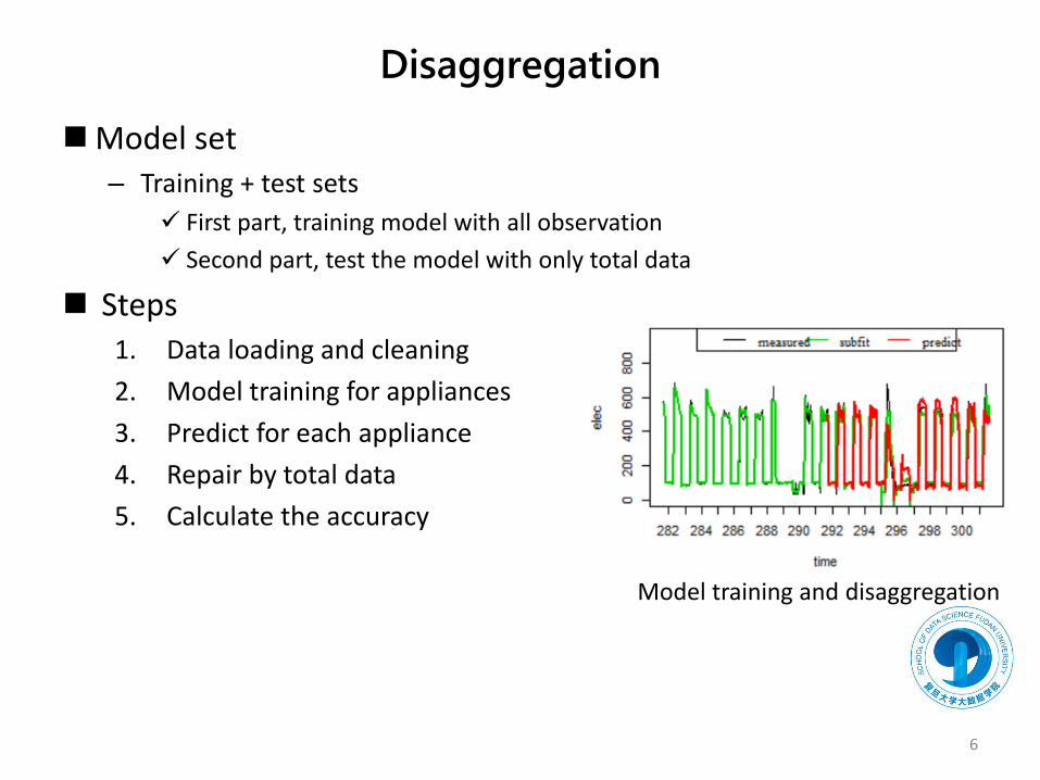
Model set– Training + test sets

First part, training model with all observation

Second part, test the model with only total data

Steps1. Data loading and cleaning

2. Model training for appliances

3. Predict for each appliance

4. Repair by total data

5. Calculate the accuracy

6

Model training and disaggregation

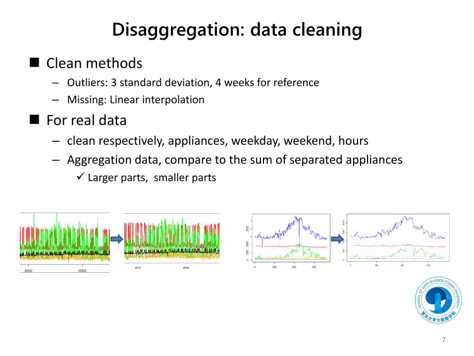
Disaggregation: data cleaning

Clean methods– Outliers: 3 standard deviation, 4 weeks for reference

– Missing: Linear interpolation

For real data– clean respectively, appliances, weekday, weekend, hours

– Aggregation data, compare to the sum of separated appliances

Larger parts, smaller parts

7

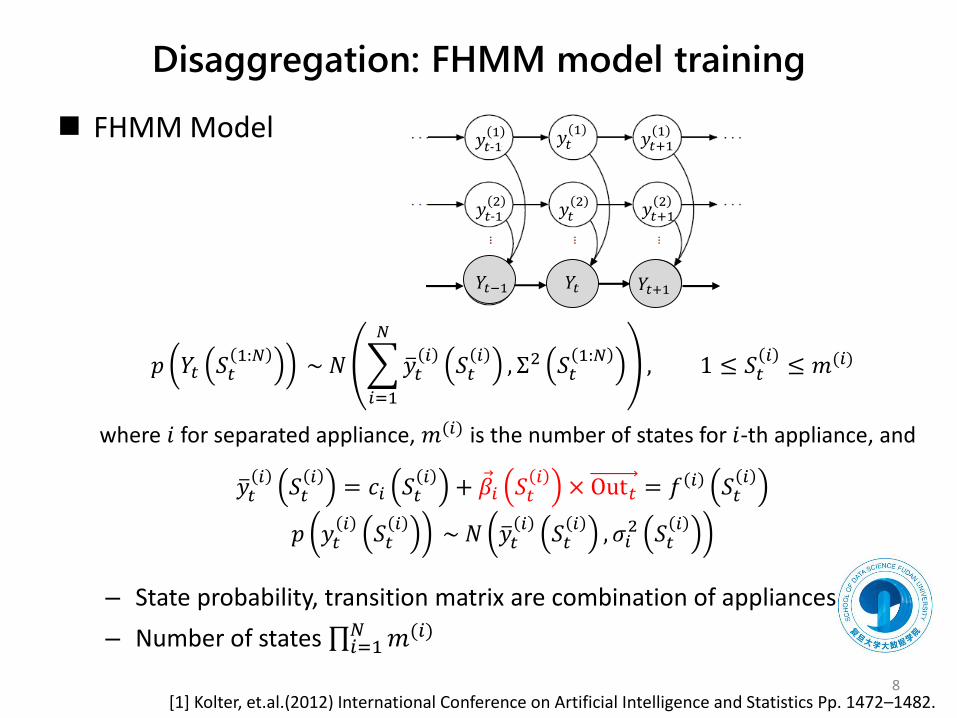
Disaggregation: FHMM model training

FHMM Model

𝑝 𝑌𝑡 𝑆𝑡1:𝑁

~ 𝑁

𝑖=1

𝑁

𝑦𝑡𝑖

𝑆𝑡𝑖

, Σ2 𝑆𝑡1:𝑁

, 1 ≤ 𝑆𝑡𝑖

≤ 𝑚(𝑖)

where 𝑖 for separated appliance, 𝑚(𝑖) is the number of states for 𝑖-th appliance, and

𝑦𝑡𝑖

𝑆𝑡𝑖

= 𝑐𝑖 𝑆𝑡𝑖

+ 𝛽𝑖 𝑆𝑡𝑖

× Out𝑡 = 𝑓 𝑖 𝑆𝑡𝑖

𝑝 𝑦𝑡𝑖

𝑆𝑡𝑖

~ 𝑁 𝑦𝑡𝑖

𝑆𝑡𝑖

, 𝜎𝑖2 𝑆𝑡

𝑖

– State probability, transition matrix are combination of appliances

– Number of states 𝑖=1𝑁 𝑚(𝑖)

8[1] Kolter, et.al.(2012) International Conference on Artificial Intelligence and Statistics Pp. 1472–1482.

𝑦𝑡2 𝑦𝑡+1

2𝑦𝑡-1

2

𝑦𝑡1

𝑦𝑡+11

𝑦𝑡-11

𝑌𝑡 𝑌𝑡+1𝑌𝑡−1

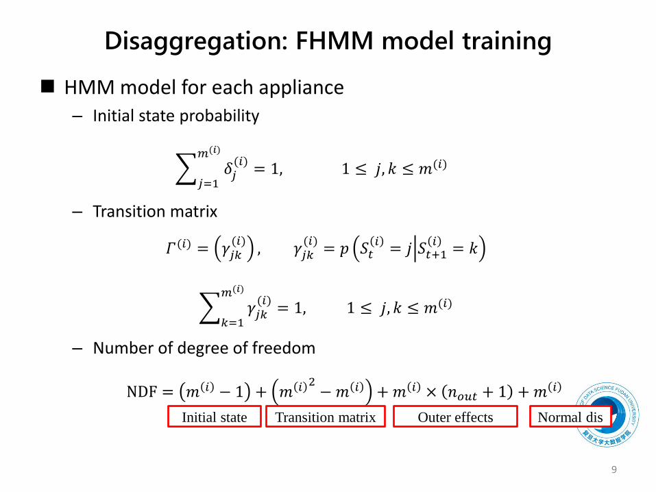
Disaggregation: FHMM model training

HMM model for each appliance– Initial state probability

𝑗=1

𝑚(𝑖)

𝛿𝑗(𝑖)

= 1, 1 ≤ 𝑗, 𝑘 ≤ 𝑚(𝑖)

– Transition matrix

𝛤(𝑖) = 𝛾𝑗𝑘(𝑖)

, 𝛾𝑗𝑘(𝑖)

= 𝑝 𝑆𝑡𝑖

= 𝑗 𝑆𝑡+1𝑖

= 𝑘

𝑘=1

𝑚(𝑖)

𝛾𝑗𝑘(𝑖)

= 1, 1 ≤ 𝑗, 𝑘 ≤ 𝑚(𝑖)

– Number of degree of freedom

NDF = 𝑚 𝑖 − 1 + 𝑚 𝑖 2− 𝑚 𝑖 + 𝑚 𝑖 × 𝑛𝑜𝑢𝑡 + 1 + 𝑚 𝑖

9

Initial state Transition matrix Outer effects Normal dis

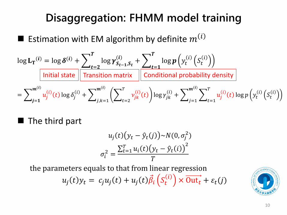
Disaggregation: FHMM model training

Estimation with EM algorithm by definite 𝑚 𝑖

log 𝐋𝐓(𝒊) = log𝜹(𝒊) +

𝒕=𝟐

𝑻

log 𝜸𝑺𝒕−𝟏,𝑺𝒕

(𝒊)+

𝒕=𝟏

𝑻

log𝒑 𝑦𝑡𝑖

𝑆𝑡𝑖

= 𝒋=𝟏

𝒎(𝒊)

𝑢𝑗𝑖

𝑡 log 𝛿𝑗𝑖

+ 𝑗,𝑘=1

𝒎(𝒊)

𝑡=2

𝑇

𝜈𝑗𝑘(𝑖)

𝑡 log 𝛾𝑗𝑘(𝑖)

+ 𝑗=1

𝒎(𝒊)

𝑡=1

𝑇

𝑢𝑗𝑖

𝑡 log 𝑝 𝑦𝑡𝑖

𝑆𝑡𝑖

The third part

𝑢𝑗 𝑡 𝑦𝑡 − 𝑦𝑡 𝑗 ~𝑁(0, 𝜎𝑗2)

𝜎𝑖2 =

𝑡=1𝑇 𝑢𝑖 𝑡 𝑦𝑡 − 𝑦𝑡 𝑖

2

𝑇

the parameters equals to that from linear regression

𝑢𝑗 𝑡 𝑦𝑡 = 𝑐𝑗𝑢𝑗 𝑡 + 𝑢𝑗 𝑡 𝛽𝑖 𝑆𝑡𝑖

× Out𝑡 + 휀𝑡(𝑗)

10

Initial state Transition matrix Conditional probability density

Disaggregation: FHMM model training

Decide the number of states 𝑚 𝑖

– Loop from 2 to 25

residual = 𝑦𝑡(𝑖)

− 𝑗=1𝑚(𝑖)

𝑦𝑡 𝑆 = 𝑗 × 𝑝(𝑆𝑡𝑖

= 𝑗) weak stable

BIC = logSSRp

𝑇+ log(𝑇)

𝑛𝑑𝑓

𝑇least

𝑦𝑡𝑖−𝑚𝑒𝑎𝑛 𝑦 𝑖

𝑠𝑑 𝑦 𝑖 < 5 no outliers

– Repeat fitting, take best fit result

11

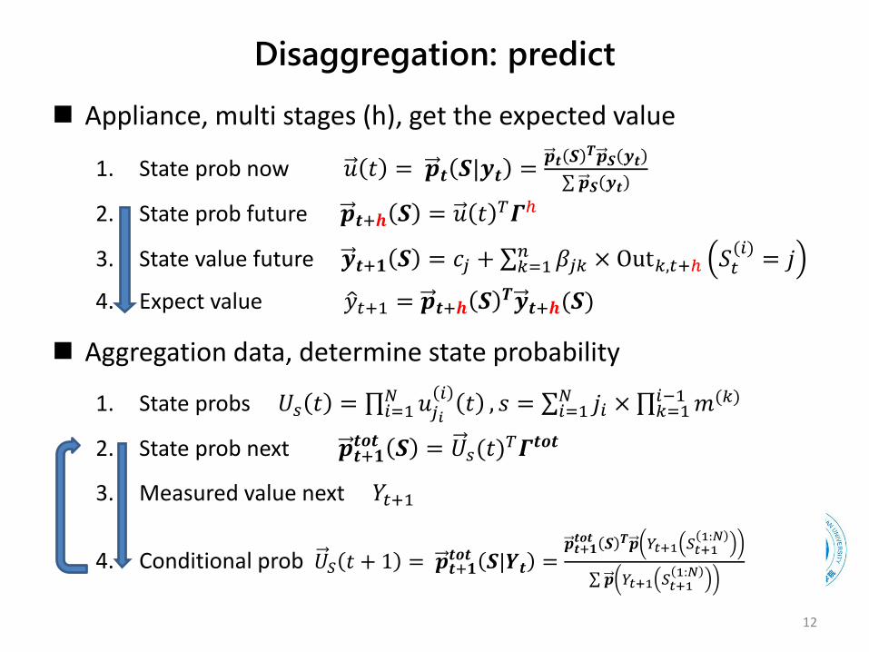
Disaggregation: predict

Appliance, multi stages (h), get the expected value

1. State prob now 𝑢 𝑡 = 𝒑𝒕 𝑺|𝒚𝒕 =𝒑𝒕 𝑺 𝑻𝒑𝑺 𝒚𝒕

𝒑𝑺 𝒚𝒕

2. State prob future 𝒑𝒕+𝒉 𝑺 = 𝑢 𝑡 𝑇𝜞ℎ

3. State value future 𝒚𝒕+𝟏 𝑺 = 𝑐𝑗 + 𝑘=1𝑛 𝛽𝑗𝑘 × Out𝑘,𝑡+ℎ 𝑆𝑡

(𝑖)= 𝑗

4. Expect value 𝑦𝑡+1 = 𝒑𝒕+𝒉 𝑺 𝑻𝒚𝒕+𝒉(𝑺)

Aggregation data, determine state probability

1. State probs 𝑈𝑠 𝑡 = 𝑖=1𝑁 𝑢𝑗𝑖

𝑖𝑡 , 𝑠 = 𝑖=1

𝑁 𝑗𝑖 × 𝑘=1𝑖−1 𝑚(𝑘)

2. State prob next 𝒑𝒕+𝟏𝒕𝒐𝒕 𝑺 = 𝑈𝑠(𝑡)

𝑇𝜞𝒕𝒐𝒕

3. Measured value next 𝑌𝑡+1

4. Conditional prob 𝑈𝑆 𝑡 + 1 = 𝒑𝒕+𝟏𝒕𝒐𝒕 𝑺|𝒀𝒕 =

𝒑𝒕+𝟏𝒕𝒐𝒕 𝑺 𝑻𝒑 𝑌𝑡+1 𝑆𝑡+1

1:𝑁

𝒑 𝑌𝑡+1 𝑆𝑡+11:𝑁

12

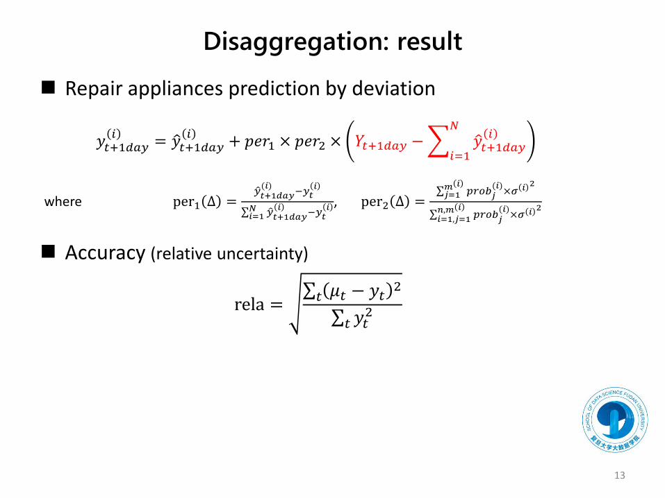
Disaggregation: result

Repair appliances prediction by deviation

𝑦𝑡+1𝑑𝑎𝑦𝑖

= 𝑦𝑡+1𝑑𝑎𝑦𝑖

+ 𝑝𝑒𝑟1 × 𝑝𝑒𝑟2 × 𝑌𝑡+1𝑑𝑎𝑦 − 𝑖=1

𝑁

𝑦𝑡+1𝑑𝑎𝑦𝑖

where per1 Δ = 𝑦𝑡+1𝑑𝑎𝑦(𝑖)

−𝑦𝑡𝑖

𝑖=1𝑁 𝑦𝑡+1𝑑𝑎𝑦

𝑖−𝑦𝑡

𝑖 , per2 Δ = 𝑗=1

𝑚 𝑖𝑝𝑟𝑜𝑏𝑗

(𝑖)×𝜎 𝑖 2

𝑖=1,𝑗=1𝑛,𝑚 𝑖

𝑝𝑟𝑜𝑏𝑗(𝑖)

×𝜎 𝑖 2

Accuracy (relative uncertainty)

rela = 𝑡 𝜇𝑡 − 𝑦𝑡

2

𝑡 𝑦𝑡2

13

Data

Electricity– Mall, office, hotel, composite

– Time: 2016-1-1 0:00 to 2016-12-31 23:00, hourly

– Measured items: total, lighting, air condition, movement, others

More– Temperature(2), raining, wind velocity, pressure, humidity

– Holiday: 10 legal holiday, 11 weekend, 00 workday;

– Day-night: dummy variable; hour, 0~23

Cleaning– Outliers

– Missing values

– Unknown = total-sum

14

Data status

Differences between buildings, sub items are small

15

Office Mall

CompositeHotel

Office

Mall

Composite

Hotel

Data status

Electricity (day night obvious, air condition season sensitive)

Comparison all

16

mall hour Total (kWh) Light (kWh) AC (kWh) Mv (kWh) Other (kWh)

Day 9-22 1200~2300 (season)

800 0-800 (season)

200 100

night 23-8 ~200 100 0 20 0

Mall Office Hotel Composite

Max (kWh) 2500 2000 3500 2500

Day 9-22 6-18 8-23 8-22

Dominant Lighting lighting Acs summer, lighting other

Acs summer, lighting other

Week cycle No Lighting, Acs, movement

Lighting Lighting

Common Air conditions sensitive to season, large fluctuation; spring festival effect obvious, difference between appliances small

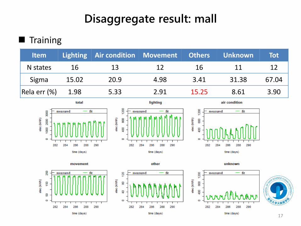
Disaggregate result: mall

Training

17

Item Lighting Air condition Movement Others Unknown Tot

N states 16 13 12 16 11 12

Sigma 15.02 20.9 4.98 3.41 31.38 67.04

Rela err (%) 1.98 5.33 2.91 15.25 8.61 3.90

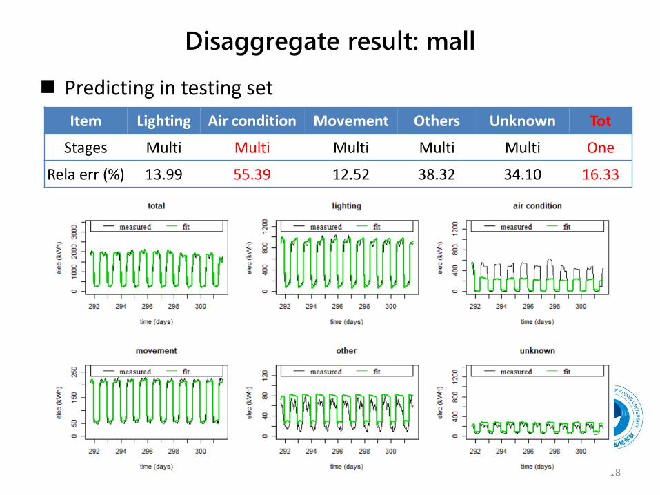
Disaggregate result: mall

Predicting in testing set

18

Item Lighting Air condition Movement Others Unknown Tot

Stages Multi Multi Multi Multi Multi One

Rela err (%) 13.99 55.39 12.52 38.32 34.10 16.33

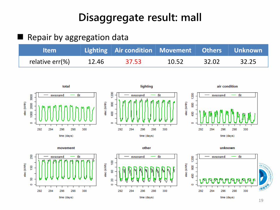
Disaggregate result: mall

Repair by aggregation data

19

Item Lighting Air condition Movement Others Unknown

relative err(%) 12.46 37.53 10.52 32.02 32.25

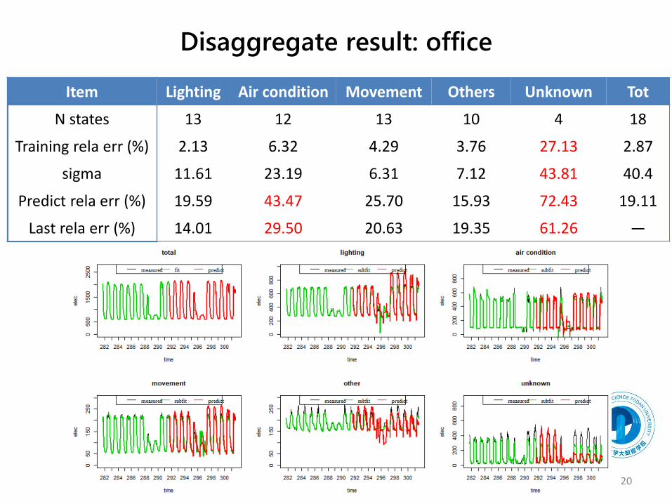
Disaggregate result: office

20

Item Lighting Air condition Movement Others Unknown Tot

N states 13 12 13 10 4 18

Training rela err (%) 2.13 6.32 4.29 3.76 27.13 2.87

sigma 11.61 23.19 6.31 7.12 43.81 40.4

Predict rela err (%) 19.59 43.47 25.70 15.93 72.43 19.11

Last rela err (%) 14.01 29.50 20.63 19.35 61.26 —

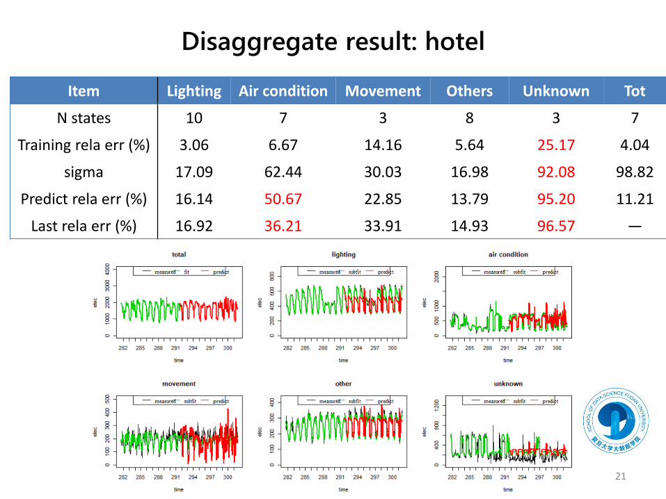
Disaggregate result: hotel

21

Item Lighting Air condition Movement Others Unknown Tot

N states 10 7 3 8 3 7

Training rela err (%) 3.06 6.67 14.16 5.64 25.17 4.04

sigma 17.09 62.44 30.03 16.98 92.08 98.82

Predict rela err (%) 16.14 50.67 22.85 13.79 95.20 11.21

Last rela err (%) 16.92 36.21 33.91 14.93 96.57 —

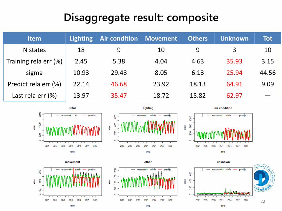
Disaggregate result: composite

22

Item Lighting Air condition Movement Others Unknown Tot

N states 18 9 10 9 3 10

Training rela err (%) 2.45 5.38 4.04 4.63 35.93 3.15

sigma 10.93 29.48 8.05 6.13 25.94 44.56

Predict rela err (%) 22.14 46.68 23.92 18.13 64.91 9.09

Last rela err (%) 13.97 35.47 18.72 15.82 62.97 —

Disaggregation comparison

Testing relative uncertainty larger than training

The larger of relative uncertainty for training, the larger disaggregation

Performance similar for buildings

Air condition, unknown largest both training and disaggregation, for large fluctuation

23

Item LightingAir

conditionMovement Others Unknown Tot

Training relative

error (%)

Mall 1.98 5.33 2.91 15.25 8.61 3.90

Office 2.13 6.32 4.29 3.76 27.13 2.87

Hotel 3.06 6.67 14.16 5.64 25.17 4.04

Composite 2.45 5.38 4.04 4.63 35.93 3.15

Result relative

error (%)

Mall 12.46 37.53 10.52 32.02 32.25 —

Office 14.01 29.50 20.63 19.35 61.26 —

Hotel 16.92 36.21 33.91 14.93 96.57 —

Composite 13.97 35.47 18.72 15.82 62.97 —

Summary

Extend FHMM model with bonus data to disaggregate hourly whole-building electricity consumption into appliances

Apply the method to several commercial buildings– Successfully disaggregate and get rules of appliances

– Performance for different buildings are similar

– Model training perfect, relative uncertainty lower than 7%

– Model testing, air condition not good for large fluctuation

Extend to similar buildings without collectors– Input the characters of buildings into the model

– Training different models for different type buildings

– Important for energy monitoring, need response, accurate prediction

24