1

MASTER THESIS

TITLE: Energy Consumption Evaluation on the MAC layer of PRCSMA

MASTER DEGREE: Master in Science in Telecommunication Engineering & Management

AUTHORS: Adamantia Stamou, Eirini Stavrou

DIRECTOR: Jesús Alonso Zárate

CO-DIRECTORS: Christos Verikoukis, Luis Alonso

DATE: September 28 th 2009

2

Overview

This thesis aims at contributing to measuring the energy consumption of PRCSMA protocol. The focus is on the evaluation of energy consumption on the medium access control (MAC) protocol of PRCSMA for an ad hoc and cooperative wireless network.

A comprehensive state of the art and a background on the topic is provided in a first part of this dissertation. Then, the contribution of the thesis is presented.

The following part of the thesis turns the focus to a specific kind of cooperative communications namely the Cooperative Automatic Retransmission Request (C-ARQ) schemes. The main idea behind C-ARQ is that when a packet is received with errors at a receiver, a retransmission can be requested not only from the source but also to any of the users which overheard the original transmission. These users can become spontaneous helpers to assist in the failed transmission by forming a temporary ad hoc network. Also, the analysis of PRCSMA protocol is presented, which is based on the IEEE 802.11 Standard. What is more, the analysis of the energy model that has been used in this study is analyzed. A comparison in energy efficiency with non-cooperative ARQ schemes (retransmissions performed only from the source) and with ideal C-ARQ (with perfect scheduling among the relays) is included under different conditions, to have actual reference benchmarks of the novel proposals. The main results show the cases that PRCSMA outperforms in terms of energy efficiency non-cooperative ARQ schemes and that the overhead of the MAC layer cannot be neglected in order to have more accurate results.

3

Contents

..................................................................................................................1 Introduction 82 State of the Art – Introduction to Network Simulators and Energy Aware Mac Protocols, Overview of 802.11 DCF and Previous Models on energy analysis on 802.11

..................................................................................................and 802.11-like protocols 10...........................................................................................2.1 Network Simulators 10

................................................................2.1.1 QualNet (similar to GloMoSim) 10...................................................................2.1.2 Network simulator (version 2) 10...................................................................2.1.3 Network simulator (version 3) 11

............................................................................2.2 Power Aware MAC Protocols 11..................................................................................2.3 Overview of IEEE 802.11 12

...........2.3.1 Description of the Architecture of the IEEE 802.11 draft standard 13..............................................................2.3.2 Medium Access Control sublayer 14

.................................................2.3.3 Distributed Coordination Function (DCF) 15......................................................................................................2.4 Related work 18

2.4.1 Description of two energy consumption models, one on 802.11 Ad-hoc ....................................................................................Networks and one on S-MAC 19

2.4.2 Description of an energy consumption model on S-MAC under different .......................................................................................................traffic conditions. 22

.......2.4.3 Description of an energy consumption model based on 802.11 DCF 25.2.4.4 Description of an energy model based on 802.11e with HCF and EDCF 28

2.4.5 Description of an energy consumption model in Single Hop IEEE 802.11 .........................................................................................................Ad Hoc network 29

2.4.6 Description of an energy consumption model of a Wireless Network .....................................................Interface in an Ad Hoc Networking Environment 33

..........................................................2.4.7 Recapitulation of the previous work 37..........................................................................................3 Contribution of the thesis 39

.................................................................................................................4 Framework 39.............................................4.1 Cooperative ARQ Scheme in Wireless Networks 40

.........................4.2 PRCSMA (Persistent Relay Carrier Sensing Multiple Access) 42................................................................5 Energy Consumption Model on PRCSMA 44

....................................................................................................5.1 System Model 44..............................................................................5.2 Energy Consumption Model 45

........................................................................5.3 Power Consumption Evaluation 51...........................................................................................................5.4 Examples 53

................................................................................6 Energy Performance Evaluation 56...............................................................................................6.1 Matlab Simulator 56................................................................................................6.1.1 Introduction 56

....................................................................................6.1.2 Transmission Rates 57

4

.........................................................................................6.1.3 Backoff Counter 58...............................................................................6.1.4 Non-cooperative ARQ 59..............................................................................6.1.5 Ideal case of PRCSMA 60

......................................................................................6.1.6 Energy Efficiency 61...............................................................................................................6.2 Results 63

........6.2.1 Packet Error Probability in the Channel from Source to Destination 63........6.2.2 Packet Error Probability in the Channel from Relays to Destination 67

................................................................................6.2.3 Length of data packet 71...........................................................6.2.4 Fairness in the energy consumption 73

....................................................6.2.5 Different values of Contention Window 75............................................................6.2.6 Different number of Active Relays 78

.....................................................................................7 Conclusions and future work 80....................................................................................................8 Acknowledgements 82

.................................................................................................................9 References 82

Index of Figures

Figure 1 Example of an Ad-hoc network................................................................ 9Figure 2. Sketch of an infrastructure network...................................................... 14Figure 3 Transmission of an MPDU with RTS/CTS............................................. 17Figure 4 Network Topology.................................................................................. 20Figure 5 Topology 1............................................................................................. 24Figure 6 Topology 2............................................................................................. 25Figure 7 System Model........................................................................................ 45Figure 8 Instantaneous power consumption vs. RF power level for various transmission rates............................................................................................... 53Figure 9 Successful transmission without relays................................................. 54Figure 10 Successful transmission from the source to the destination with one relay..................................................................................................................... 54Figure 11 Transmission from the source to the destination with one relay containing an error............................................................................................... 55Figure 12 Energy Efficiency for =0.1 and potential relays=10...................... 63

Figure 13 Energy Efficiency for =0.1 and potential relays=10....................... 64

Figure 14 Energy Efficiency for =0.1 and potential relays=1......................... 65

Figure 15 Energy Efficiency for =0.7 and potential relays=10....................... 67

Figure 16 Energy Efficiency for =0.1 and potential relays=10....................... 68

5

Figure 17 Energy Efficiency for =0.7 and potential relays=10....................... 70

Figure 18 Energy Efficiency for =0.1 and potential relays=1......................... 70

Figure 19 Energy Efficiency for =0.7 and potential relays=1......................... 71

Figure 20 Energy Efficiency for =0.1, =0.7, Potential Relays=1.............. 72

Figure 21 Energy Efficiency for =0.1, =0.7, Potential Relays=10............ 73

Figure 22 Energy Efficiency for 1 active relay as a function of the contention window................................................................................................................. 77Figure 23 Energy Efficiency for 5 active relays as a function of the contention window................................................................................................................. 78Figure 24 Energy Efficiency for 15 active relays as a function of the contention window................................................................................................................. 78Figure 25 Energy Efficiency as a function of the number of relays..................... 80

List of Acronyms

ACK AcknowledgmentACs Access CategoriesAP Access Point ARQ Automatic Retransmission/Repeat RequestBEB Binary Exponential Backoff BSA Basic Service AreaC-ARQ Cooperative ARQ CBQ Class Based QueueingCBR Constant Bit RateCDMA Code division multiple accessCFP Contention-Free Period COLAV Collision Avoidance ModeCP Contention Period CSMA/CA Carrier Sensing Multiple Access with Collision Avoidance CTS Clear To SendCW Contention WindowDCF Distributed Coordination FunctionDIFS DCF Inter Frame SpaceED Error Detection EDCF Enhanced Distributed Control FunctionEIFS Extended Inder Frame SpaceESS Extended Service Set

6

FDDI Fiber Distributed Data Interface FDMA Frequency Division Multiple Access FEC Forward Error Correction FTP File Transfer ProtocolGloMoSim Global Mobile Information System SimulatorGNU GNU's Not UnixGPLv2 General Public License version2HCF Hybrid Coordination FunctionIFS Interframe Space LAN Local Area NetworkLLC Logical Link Control MAC Medium Access ControlMAN Metropolitan Area Network MinGW Minimalist GNU for WindowsMPDU MAC Protocol Data UnitMSDUs MAC Service Data Units NACK Negative AcknowledgmentNAV Network Allocation VectorNAV Network Allocation VectorNIC Network Interface CardNLOS No Line-Of-Sight ns-2 Network simulator (version 2)ns-3 Network simulator (version 3)OFDMA Orthogonal Frequency-Division Multiple AccessOS X Operating System XOTcl Tcl script language with Object-oriented extensionsPCMCIA Personal Computer Memory Card International AssociationPHY Physical LayerPRCSMA Persistent Relay Carrier Sensing Multiple AccessQoS Quality of ServiceRCR Relay Control Rate RDR Relay Data Rate RED Random Early Detection)RF Radio FrequencyRTS Request To SendSCR Source Control Rate SDR Source Data Rate SIFS Short Inter Frame SpaceSMAC Sensor MACSNR Signal to Noise RatioSYNC Synchronization TCP Transmission Control ProtocolTCs Traffic CategoriesTDMA Time Division Multiple AccessTelnet Teletype Network ProtocolT-MAC Timeout MAC

7

TRAMA Traffic-Adaptive Medium Access ProtocolUC University of CaliforniaUPD User Datagram ProtocolUPs User PriorityVB Variant Bit RateWLAN Wireless Local Area Network

1 Introduction

IEEE 802.11 based devices are gaining popularity. Although technologies in wireless physical layer have been advanced in the recent years and it continues to be in progress, mobile devices are dependent on battery power. One of the most major issues in wireless networks is the energy consumption because it limits the lifetime of the terminals, and consequently the lifetime of the whole network.

It is considered that the bottleneck situation of battery life will continue in the coming years. As a result, it is really important to calculate the energy consumption of a network in order to minimize it.

Modeling and simulating from the energy consumption point of view, is not only a good method to measure the energy consumption, but also provides insights into how to choose parameters to improve the energy efficiency. Furthermore, the power consumption of a network interface can be significant, especially for small devices, where the need of energy minimization is essential.

Many studies have demonstrated that the radio activity of a WLAN (Wireless Local Area Network), controlled by the MAC (Medium Access Control) layer, consumes an important part of the energy. So, in this project, our goal is to evaluate the energy efficiency of PRCSMA (Persistent Relay Carrier Sensing

8

Multiple Access) and in second level to improve the energy consumption of the protocol by adding a low consumption mode.

As we will further discuss in the following chapters, PRCSMA is an 802.11-based protocol which is a MAC protocol for wireless Ad-hoc networks that allows executing a distributed and cooperative ARQ (Automatic Retransmission reQuest) scheme.

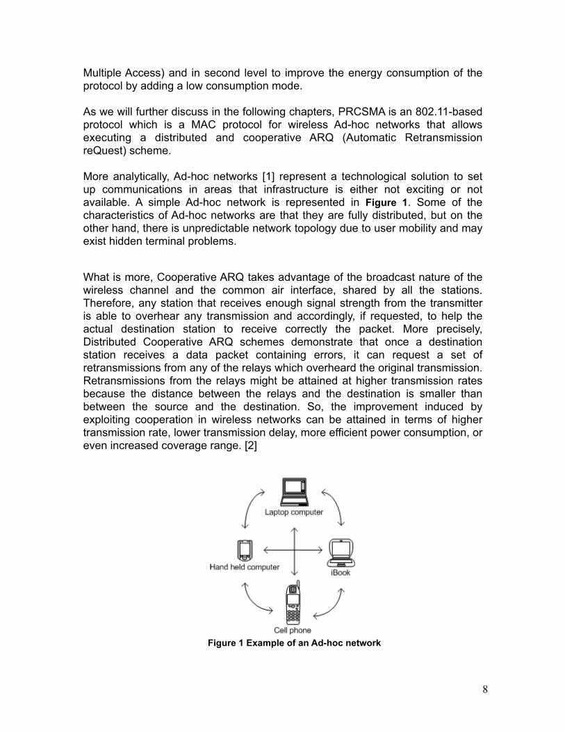
More analytically, Ad-hoc networks [1] represent a technological solution to set up communications in areas that infrastructure is either not exciting or not available. A simple Ad-hoc network is represented in Figure 1. Some of the characteristics of Ad-hoc networks are that they are fully distributed, but on the other hand, there is unpredictable network topology due to user mobility and may exist hidden terminal problems.

What is more, Cooperative ARQ takes advantage of the broadcast nature of the wireless channel and the common air interface, shared by all the stations. Therefore, any station that receives enough signal strength from the transmitter is able to overhear any transmission and accordingly, if requested, to help the actual destination station to receive correctly the packet. More precisely, Distributed Cooperative ARQ schemes demonstrate that once a destination station receives a data packet containing errors, it can request a set of retransmissions from any of the relays which overheard the original transmission. Retransmissions from the relays might be attained at higher transmission rates because the distance between the relays and the destination is smaller than between the source and the destination. So, the improvement induced by exploiting cooperation in wireless networks can be attained in terms of higher transmission rate, lower transmission delay, more efficient power consumption, or even increased coverage range. [2]

Figure 1 Example of an Ad-hoc network

9

The rest of the dissertation is organized as follows. Ιn the literature, there exists a family of different models on energy analysis of IEEE 802.11 and 802.11-like protocols [3]-[9]. For completeness, they are overviewed in the following chapter plus the overview of the 802.11 DCF protocol. The main contributions of this thesis are presented in Chapter 3. The framework of the thesis is presented in Chapter 4, where the C-ARQ and the PRSCMA protocol are analysed. In Chapter 5, the energy model on PRSCMA is presented, including the system model, the power consumption evaluation and examples on energy consumption of PRCSMA. What is more, in Chapter 6, the energy performance evaluation is presented, focusing on the Matlab simulator and the results that we accomplished from the simulations under different scenarios. Furthermore, in Chapter 7, the conclusions of the thesis and future work are discussed. Finally in Chapter 8 and in Chapter 9, the acknowledgments and the references are presented respectively.

2 State of the Art – Introduction to Network Simulators and Energy Aware Mac Protocols, Overview of 802.11 DCF and Previous Models on energy analysis on 802.11 and 802.11-like protocols

In this section the network simulators QualNet, ns-2 and ns-3 are presented. Also, the power aware MAC protocols that are used in the energy models presented above are defined and follow the overview of 802.11 DCF protocol and the related work.

2.1 Network Simulators

A short introduction to network simulators used by the proposed articles ([3]-[9]), will help the reader to have a clearer and wider view on the following energy consumption models and the relative simulations.

2.1.1 QualNet (similar to GloMoSim)

10

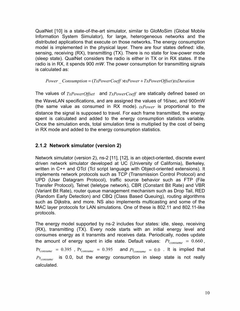
QualNet [10] is a state-of-the-art simulator, similar to GloMoSim (Global Mobile Information System Simulator), for large, heterogeneous networks and the distributed applications that execute on those networks. The energy consumption model is implemented in the physical layer. There are four states defined: idle, sensing, receiving (RX), transmitting (TX). There is no state for low-power mode (sleep state). QualNet considers the radio is either in TX or in RX states. If the radio is in RX, it spends 900 mW. The power consumption for transmitting signals is calculated as:

The values of and are statically defined based on the WaveLAN specifications, and are assigned the values of 16/sec, and 900mW (the same value as consumed in RX mode). is proportional to the distance the signal is supposed to travel. For each frame transmitted, the energy spent is calculated and added to the energy consumption statistics variable. Once the simulation ends, total simulation time is multiplied by the cost of being in RX mode and added to the energy consumption statistics.

2.1.2 Network simulator (version 2)

Network simulator (version 2), ns-2 [11], [12], is an object-oriented, discrete event driven network simulator developed at UC (University of California), Berkeley, written in C++ and OTcl (Tcl script language with Object-oriented extensions). It implements network protocols such as TCP (Transmission Control Protocol) and UPD (User Datagram Protocol), traffic source behavior such as FTP (File Transfer Protocol), Telnet (teletype network), CBR (Constant Bit Rate) and VBR (Variant Bit Rate), router queue management mechanism such as Drop Tail, RED (Random Early Detection) and CBQ (Class Based Queuing), routing algorithms such as Dijkstra, and more. NS also implements multicasting and some of the MAC layer protocols for LAN simulations. One of these is 802.11 and 802.11-like protocols.

The energy model supported by ns-2 includes four states: idle, sleep, receiving (RX), transmitting (TX). Every node starts with an initial energy level and consumes energy as it transmits and receives data. Periodically, nodes update the amount of energy spent in idle state. Default values: ,

, and . It is implied that

is 0.0, but the energy consumption in sleep state is not really

calculated.

11

2.1.3 Network simulator (version 3)

Network simulator (version 3), ns-3 is a discrete-event network simulator for Internet systems, targeted primarily for research and educational use. ns-3 is free software, licensed under the GNU (GNU's Not Unix) GPLv2 (General Public License version2) license, and is publicly available for research, development, and use. Ns-3 is intended as an eventual replacement for the popular ns-2 simulator. The project acronym “nsnam” derives historically from the concatenation of ns (network simulator) and nam (network animator). This network simulator is written in C++ and Python and is available as source code releases for Linux and Unix variants, OS X, and Windows via Cygwin (Linux-like environment for Windows) or MinGW (Minimalist GNU for Windows).

2.2 Power Aware MAC Protocols

Sensor MAC (SMAC) S-MAC [13] is a modification of IEEE 802.11 protocol specifically designed for sensor networks. It was developed with power saving as one of its design goals. Its advantage is that it supports low-power radio mode. Nodes alternate between periodic sleep and listen periods. Listen periods are split into synchronization and data periods. During synchronization periods, nodes broadcast their sleeping schedule, and, based on the information received from neighbors, they adjust their schedule so that they all sleep at the same time. This composes a virtual cluster of neighboring nodes. A complete cycle of listen and sleep is called a frame in S-MAC (Sensor MAC).

During data periods, a node with data to send will contend for the medium Request_to_Send – Clear_to_Send exchange (RTS-CTS). If the node acquires the medium or if it has data to receive, it will not sleep in the next period and the data will be exchanged. After that, if there is still enough time in the sleep period, the node goes to sleep. If a node does not have data to transmit or receive, it will sleep.

What is more, S-MAC proposed a message passing mechanism which allows a number of fragments for a message to be transmitted with only one RTS and CTS. In this way the number of control packets has been reduced. A disadvantage of this protocol is that in order to saves energy it sacrifices latency.

Also, there are some other power aware MAC protocols such as T-MAC (Timeout MAC) [14] which uses an active/sleep duty cycle and TRAMA (traffic-adaptive medium access protocol) [15]. The latter is a power aware scheduled-based (time slotted) MAC Protocol. Its advantage is that it schedules transmission being self adaptive to changes in traffic, node state or connectivity.

12

2.3 Overview of IEEE 802.11

Wireless computing is a rapidly emerging technology providing users with network connectivity without being tethered off a wired network. Wireless local area networks (WLANs), like their wired counterparts, are being developed to provide high bandwidth to users in a limited geographical area. WLANs are being studied as an alternative to the high installation and maintenance costs incurred by traditional additions, detections, and changes experienced in wired LAN infrastructures. [16]

The protocol which is under investigation in the thesis is the wireless PRCSMA. The scope of this thesis is the calculation of the energy consumption of a network whose function is based on this protocol. This protocol is based on the standard 802.11.

The MAC functional description is presented in this clause. The architecture of the MAC sublayer, including the distributed coordination function (DCF), the point coordination function (PCF), and their coexistence in an IEEE 802.11 LAN are introduced. These functions are expanded and a complete functional description of each is provided. Fragmentation and defragmentation are also covered. Multirate support is addressed. The allowable frame exchange sequences are listed. Finally, a number of additional restrictions to limit the cases in which MSDUs are reordered or discarded are described.

2.3.1 Description of the Architecture of the IEEE 802.11 draft standard

The fundamental block of the IEEE 802.11 architecture is defined as BSS which means Basic Service Set. A BSS is a group of stations that are under the direct control of a single coordination function (i.e., a DCF or PCF) We are interesded in the DCF which is described below. The geographical area covered by the BSS is known as the basic service area (BSA), which is analogous to a cell in a cellular communications network. All stations in a BSS can communicate directly with all other stations in a BSS. However, transmission medium degradations due to multipath fading, or interference from nearby BSSs reusing the same physical-layer characteristics (e.g., frequency and spreading code, or hopping pattern), can cause some stations to appear “hidden” from other stations.

An intentional grouping of stations exists into a single BSS for the purposes of internet worked communications without the aid of an infrastructure network and is defined as an ad hoc network. Any station can establish a direct communications session with any other station in the BSS, without the

13

requirement of channeling all traffic through a centralized access point (AP).

Infrastructure networks are established to provide wireless users with specific services and range extension. They are in the context of IEEE 802.11 are established using APs. The AP is analogous to the base station in a cellular communications network. The AP supports range extension by providing the integration points necessary for network connectivity between multiple BSSs, thus forming an extended service set (ESS). The ESS has the appearance of one large BSS to the logical link control (LLC) sublayer of each station (STA). Several BSSs that are integrated together using a common distribution system (DS) create the ESS. The DS can be thought of as a backbone network that is responsible for MAC-level transport of MAC service data units (MSDUs). The DS, as specified by IEEE 802.11, is implementation independent. Therefore, the DS could be a wired IEEE 802.3 token bus LAN, IEEE 802.5 token ring LAN, fiber distributed data interface (FDDI) metropolitan area network (MAN), or another IEEE 802.11 wireless medium. Note that while the DS could physically be the same transmission medium as the BSS, they are logically different, because the DS is solely used as a transport backbone to transfer packets between different BSSs in the ESS. An ESS can also provide gateway access for wireless users into a wired network such as the Internet. This is accomplished via a device known as a portal.

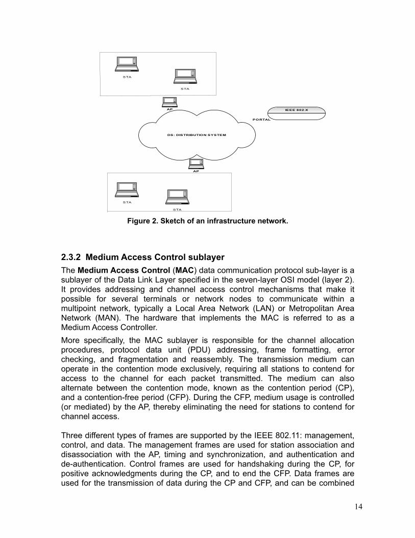
The portal is a logical entity that specifies the integration point on the DS where the IEEE 802.11 network integrates with a non-IEEE 802.11 network. If the network is an IEEE 802.X, the portal incorporates functions which are analogous to a bridge; that is, it provides range extension and the translation between different frame formats. Figure 2 illustrates a simple ESS developed with two BSSs, a DS, and a portal access to a wired LAN.

14

Figure 2. Sketch of an infrastructure network.

2.3.2 Medium Access Control sublayerThe Medium Access Control (MAC) data communication protocol sub-layer is a sublayer of the Data Link Layer specified in the seven-layer OSI model (layer 2). It provides addressing and channel access control mechanisms that make it possible for several terminals or network nodes to communicate within a multipoint network, typically a Local Area Network (LAN) or Metropolitan Area Network (MAN). The hardware that implements the MAC is referred to as a Medium Access Controller.More specifically, the MAC sublayer is responsible for the channel allocation procedures, protocol data unit (PDU) addressing, frame formatting, error checking, and fragmentation and reassembly. The transmission medium can operate in the contention mode exclusively, requiring all stations to contend for access to the channel for each packet transmitted. The medium can also alternate between the contention mode, known as the contention period (CP), and a contention-free period (CFP). During the CFP, medium usage is controlled (or mediated) by the AP, thereby eliminating the need for stations to contend for channel access.

Three different types of frames are supported by the IEEE 802.11: management, control, and data. The management frames are used for station association and disassociation with the AP, timing and synchronization, and authentication and de-authentication. Control frames are used for handshaking during the CP, for positive acknowledgments during the CP, and to end the CFP. Data frames are used for the transmission of data during the CP and CFP, and can be combined

15

with polling and acknowledgments during the CFP.

2.3.3 Distributed Coordination Function (DCF)

The access method which is used in the IEEE 802.11 is a DCF known as carrier sense multiple access with collision avoidance (CSMA/CA). The DCF is the fundamental MAC technique of the IEEE 802.11 wireless LAN standard. It is used to support asynchronous data transfer on a best effort basis and operates solely in the ad hoc network, and either operates solely or coexists with the PCF in an infrastructure network.

Contention services imply that each station with an MSDU queued for transmission must contend for access to the channel and, once the MSDU is transmitted, must recounted for access to the channel for all subsequent frames. Contention services promote fair access to the channel for all stations. DCF employs a CSMA/CA (Carrier Sensing Multiple Access with Collision Avoidance) distributed algorithm and an optional virtual carrier sense using RTS and CTS control frames.CSMA/CD (collision detection) is not used because a station is unable to listen to the channel for collisions while transmitting. In IEEE 802.11, carrier sensing is performed at both the air interface, referred to as physical currier sensing, and at the MAC sublayer, referred to as virtual carrier sensing.

The virtual carrier sensing is performed when MPDU (MAC Protocol Data Unit) duration information of short Request-to-send (RTS) and Clear-to-send (CTS) frames between source and destination stations are exchanged during the intervals between the data frame transmissions. The MPDU contains header information, payload, and a 32-bit CRC. The duration field indicates the amount of time (in microseconds) after the end of the present frame the channel will be utilized to complete the successful transmission of the data management frame. Stations in the BSS use the information in the duration field to adjust their network allocation vector (NAV), which indicates the amount of time that must elapse until the current transmission session is complete and the channel can be sampled again for idle status. The channel is marked busy if either the physical or virtual carrier sensing mechanisms indicate the channel is busy.

Priority access to the wireless medium is controlled through the use of interframe space (IFS) time intervals between the transmissions of frames. The IFS intervals are mandatory periods of idle time on the transmission medium. Three IFS intervals are specified in the standard: short IFS (SIFS), point coordination function IFS (PIFS), and DCF-IFS (DIFS). The SIFS interval is the smallest IFS, followed by DIFS, respectively. Stations only required to wait a SIFS have priority access over those stations required to wait a DIFS before transmitting; therefore, SIFS has the highest-priority access to the communications medium.

According to the basic access method the station which needs to transmit an

16

MPDU senses the channel. If the channel is idle the station waits for a DIFS period and then senses the channel again. In the case that the channel is still idle, the station transmits the MPDU. The receiver calculates the checksum and determines if the packet was received correctly. Finally, if the transmission was correct, the receiving station waits for a SIFS period and then transmits an acknowledgment frame (ACK) which indicates that the transmission was successful. When the data frame is transmitted, the duration field of the frame is used to let all stations in the BSS know how long the medium will be busy. All stations hearing the data frame adjust their NAV based on the duration field value, which includes the SIFS interval and the ACK following the data frame.

Because of the fact that a source cannot hear its own transmissions, a collision occurs, the source continues transmitting the complete MPDU. If the MPDU is large (e.g., 2300 octets), a lot of channel bandwidth is wasted due to a corrupt MPDU. RTS and CTS control frames can be used by a station to reserve channel bandwidth prior to the transmission of an MPDU and to minimize the amount of bandwidth wasted when collisions occur. RTS and CTS control frames are relatively small (RTS is 20 octets and CTS is 14 octets) when compared to the maximum data frame size (2346 octets). The RTS control frame is first transmitted by the source station (after success- fully contending for the channel) with a data or management frame queued for transmission to a specified destination station. All stations in the BSS, hearing the RTS packet, read the duration field and set their NAVs accordingly. The destination station responds to the RTS packet with a CTS packet after an SIFS idle period has elapsed. Stations hearing the CTS packet look at the duration field and again update their NAV (Network Allocation Vector). Upon successful reception of the CTS, the source station is virtually assured that the medium is stable and reserved for successful transmission of the MPDU.

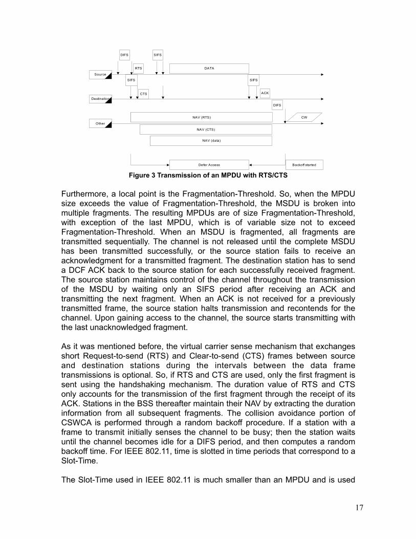
A significant point is that stations are capable of updating their NAVs based on the RTS from the source station and CTS from the destination station. That helps to be struggled the problem of the “hidden terminal”. Figure 3 illustrates the transmission of an MPDU using the RTS/CTS mechanism. Stations can choose to never use RTS/CTS, use RTS/CTS whenever the MSDU exceeds the value of RTS-Threshold (manageable parameter), or always use RTS/CTS. If a collision occurs with an RTS or CTS MPDU, far less bandwidth is wasted when compared to a large data MPDU. However, for a lightly loaded medium, additional delay is imposed by the overhead of the RTS/CTS frames. Large MSDUs handed down from the LLC to the MAC may require fragmentation to increase transmission reliability. To determine whether to perform fragmentation, MPDUs are compared to the manageable parameter.

17

Figure 3 Transmission of an MPDU with RTS/CTS

Furthermore, a local point is the Fragmentation-Threshold. So, when the MPDU size exceeds the value of Fragmentation-Threshold, the MSDU is broken into multiple fragments. The resulting MPDUs are of size Fragmentation-Threshold, with exception of the last MPDU, which is of variable size not to exceed Fragmentation-Threshold. When an MSDU is fragmented, all fragments are transmitted sequentially. The channel is not released until the complete MSDU has been transmitted successfully, or the source station fails to receive an acknowledgment for a transmitted fragment. The destination station has to send a DCF ACK back to the source station for each successfully received fragment. The source station maintains control of the channel throughout the transmission of the MSDU by waiting only an SIFS period after receiving an ACK and transmitting the next fragment. When an ACK is not received for a previously transmitted frame, the source station halts transmission and recontends for the channel. Upon gaining access to the channel, the source starts transmitting with the last unacknowledged fragment.

As it was mentioned before, the virtual carrier sense mechanism that exchanges short Request-to-send (RTS) and Clear-to-send (CTS) frames between source and destination stations during the intervals between the data frame transmissions is optional. So, if RTS and CTS are used, only the first fragment is sent using the handshaking mechanism. The duration value of RTS and CTS only accounts for the transmission of the first fragment through the receipt of its ACK. Stations in the BSS thereafter maintain their NAV by extracting the duration information from all subsequent fragments. The collision avoidance portion of CSWCA is performed through a random backoff procedure. If a station with a frame to transmit initially senses the channel to be busy; then the station waits until the channel becomes idle for a DIFS period, and then computes a random backoff time. For IEEE 802.11, time is slotted in time periods that correspond to a Slot-Time.

The Slot-Time used in IEEE 802.11 is much smaller than an MPDU and is used

18

to define the IFS intervals and determine the backoff time for stations in the CP. It is different for each physical layer implementation. The random backoff time is an integer value that corresponds to a number of time slots. Initially, the station computes a backoff time in the range 0-7. After the medium becomes idle after a DIFS period, stations decrement their backoff timer until the medium becomes busy again or the timer reaches zero. If the timer has not reached zero and the medium becomes busy, the station freezes its timer. When the timer is finally decremented to zero, the station transmits its frame. If two or more stations decrement to zero at the same time, a collision will occur, and each station will have to generate a new backoff time in the range 0-15. For each retransmission attempt, the backoff time grows as

,

where i, is the number of consecutive times a station attempts to send an MPDU, ranf() is a uniform random variety in (0,1), and represents the

largest integer less than or equal to . The idle period after a DIFS

period is referred to as the contention window (CW).

The advantage of this channel access method is that it promotes fairness among stations, but its weakness is that it probably could not support time-bounded services. Fairness is maintained because each station must re-contend for the channel after every transmission of an MSDU. All stations have equal probability of gaining access to the channel after each DIFS interval. Time-bounded services typically support applications such as packetized voice or video that must be maintained with a specified minimum delay. With DCF, there is no mechanism to guarantee minimum delay to stations supporting time-bounded services.

In the next section, some power aware protocols are introduced, which are used by the energy models presented in Section 2.4.

2.4 Related work

The purpose of this section is to present several energy models and to compare them, before analyze the energy model that we chose to investigate the energy consumption and more precisely the energy efficiency of PRCSMA. In the following paragraph, an energy model is presented, based on 802.11, which considers different radio states.

19

Frequently, the performance of network protocols is carried out using network simulators like ns-2, GloMoSim (Global Mobile Information System Simulator), QualNet. The disadvantage is that the models employed are not accurate because not all the radio states or the different energy levels are considered and the energy consumption is not automatically measured. So, in [3], a new approach is introduced for network simulators, computing more accurate the energy consumption for Ad-Hoc network protocols. The advantages of this particular energy models (802.11 DCF (Distributed Coordination Function) and S-MAC) are the consideration of all the possible radio states (including sleep state for the S-MAC) and that the simulator can compute the energy automatically irrespective of what layer of the stack the protocol designer is working. Although, a disadvantage is that they do not taking into account other delays, as the IFS time or the backoff period.

2.4.1 Description of two energy consumption models, one on 802.11 Ad-hoc Networks and one on S-MAC

The proposed energy model considers all possible radio operation modes, namely Transmitting, when radio is transmitting data, Receiving, when radio is effectivelyreceiving data, Overhearing, when radio is receiving data that is not destined to the node, Idle, when radio is ready to receive or transmit, Sensing, when radio has detected some signal, but is not able to receive it, Sleeping, when radio is in low power, and this is not able to receive or transmit. Note that sensing and overhearing states are a special case of the receiving state. The power can be calculated using , where and are the voltage and current specific to the radio. The time the radio spends in a certain state depends on the packet size and the transmission rate and is given by: . Thus, for each state, energy consumption is calculated as

where represents the power dissipated by the radio while in state , and

represents the time spent in state .

Implementation

The energy model was implemented at the radio/physical layer of both GloMoSim and QualNet. The implementation includes: (1) the necessary physical layer infrastructure to account for all possible radio modes (as specified above), and (2) an interface between the physical- and MAC layers to control the radio modes (e.g., switch radio on/off, overhearing versus reception, etc.). The physical

20

layer support for the energy consumption instrumentation includes: (1) the addition of the SLEEP state, (2) addition of a data structure for the energy model, (3) and implementation of energy consumption accounting functions.

Functions and are used for MAC layer to set the radio state to and from sleep mode. Also interaction between PHY (Physical layer) and MAC layer is needed to recognize if a received packet is in fact received or overheard. Thus, the energy model a s s u m e s t h a t a l l r e c e i v e d p a c k e t s a r e o v e r h e a r d a n d p l u s

should be used every time a received packet is destined to the node. Also, each time the radio changes state energy consumption info is updated by . Through a configuration file, the user defines the energy consumption parameters. Statistics provided by the energy model include: total energy consumption, energy consumption per state, time spent in each state (including or not a “warm up” period).

Analytical Model for 802.11

The default values for all parameters in the configuration file of QualNet were used, i.e., the transmission rate is set at 11 Mbps, and the power consumption is 900 mW for both receiving/idle and transmitting states. The transmission range for each node is 100m (receiver threshold is -75dB). CBR traffic is generated from node 0 to 2 40 times with 5 second interval; the data size is 200 bytes. A simulation run lasts 250 seconds.

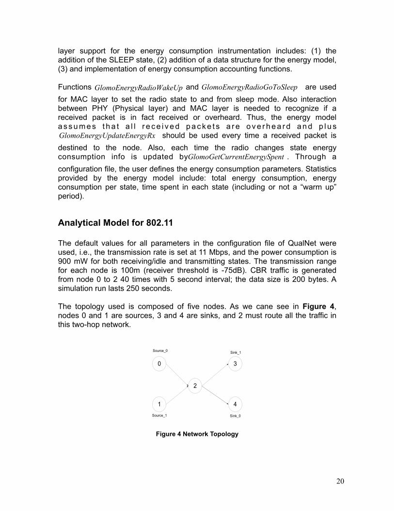
The topology used is composed of five nodes. As we cane see in Figure 4, nodes 0 and 1 are sources, 3 and 4 are sinks, and 2 must route all the traffic in this two-hop network.

Figure 4 Network Topology

21

Node Transmitted Received Overhears

0

1

2

3

4

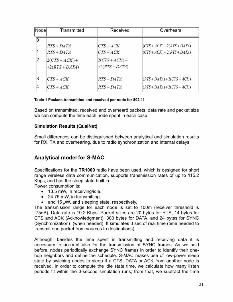
Table 1 Packets transmitted and received per node for 802.11

Based on transmitted, received and overheard packets, data rate and packet size we can compute the time each node spent in each case.

Simulation Results (QualNet)

Small differences can be distinguished between analytical and simulation results for RX, TX and overhearing, due to radio synchronization and internal delays.

Analytical model for S-MAC

Specifications for the TR1000 radio have been used, which is designed for short range wireless data communication, supports transmission rates of up to 115.2 Kbps, and has the sleep state built in. Power consumption is:

• 13.5 mW, in receiving/idle, • 24.75 mW, in transmitting • and 15 µW, and sleeping state, respectively.

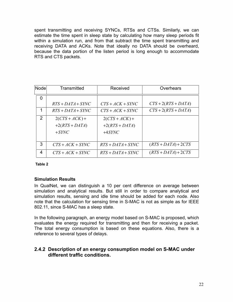
The transmission range for each node is set to 100m (receiver threshold is -75dB). Data rate is 19.2 Kbps. Packet sizes are 20 bytes for RTS, 14 bytes for CTS and ACK (Acknowledgment), 380 bytes for DATA, and 24 bytes for SYNC (Synchronization) (when needed). It simulates 3 sec of real time (time needed to transmit one packet from sources to destinations).

Although, besides the time spent in transmitting and receiving data it is necessary to account also for the transmission of SYNC frames. As we said before, nodes periodically exchange SYNC frames in order to identify their one-hop neighbors and define the schedule. S-MAC makes use of low-power sleep state by swiching nodes to sleep if a CTS, DATA or ACK from another node is received. In order to compute the idle state time, we calculate how many listen periods fit within the 3-second simulation runs; from that, we subtract the time

22

spent transmitting and receiving SYNCs, RTSs and CTSs. Similarly, we can estimate the time spent in sleep state by calculating how many sleep periods fit within a simulation run, and from that subtract the time spent transmitting and receiving DATA and ACKs. Note that ideally no DATA should be overheard, because the data portion of the listen period is long enough to accommodate RTS and CTS packets.

Node Transmitted Received Overhears

0RTS DATA SYNC+ + CTS ACK SYNC+ + 2( )CTS RTS DATA+ +

1 RTS DATA SYNC+ + CTS ACK SYNC+ + 2( )CTS RTS DATA+ +

2 2( )2( )CTS ACKRTS DATA

SYNC

+ ++ ++

2( )

2( )4

CTS ACKRTS DATASYNC

+ ++ ++

3 CTS ACK SYNC+ + RTS DATA SYNC+ + ( ) 2RTS DATA CTS+ +

4 CTS ACK SYNC+ + RTS DATA SYNC+ + ( ) 2RTS DATA CTS+ +

Table 2

Simulation ResultsIn QualNet, we can distinguish a 10 per cent difference on average between simulation and analytical results. But still in order to compare analytical and simulation results, sensing and idle time should be added for each node. Also note that the calculation for sensing time in S-MAC is not as simple as for IEEE 802.11, since S-MAC has a sleep state.

In the following paragraph, an energy model based on S-MAC is proposed, which evaluates the energy required for transmitting and then for receiving a packet. The total energy consumption is based on these equations. Also, there is a reference to several types of delays.

2.4.2 Description of an energy consumption model on S-MAC under different traffic conditions.

23

The paper [4] presents an analytic model for evaluating the energy consumption at nodes in an S-MAC based wireless sensor network, and they developed an energy consumption analysis under different traffic conditions for distinct network topologies. Plus, to validate the accuracy of the analytic model they have compared the analytic results with ns-2 simulation result. The advantage of this energy model is that it considers also IFS (Inter Frame Space) times and the results generated by the proposed model are quite approaching to the simulation results.

S-MAC Analytic Model

Four possible power modes: transmitting, receiving, idle, and sleep mode have been considered in this model. Considering a time interval of period t, total energy consumption of a node running S-MAC during t can be expressed as

Where is the number of times a node transmits a packet during , is

the corresponding for receiving, represents energy consumption of

transmitting a packet, the corresponding for receiving, the time in sleep

mode, the time in idle mode, the power consumption of sleep mode and

the power consumption of idle mode.

When a node has a packet to transmit, carrier sense delay ( ), backoff delay

( ), transmission delay, propagation delay, processing delay, queuing delay,

and sleep delay ( ) will be considered. All the delays are the same as IEEE

802.11 protocol except sleep delay.

Carrier sense delay is introduced when the sender performs carrier sense. Its value is determined by the contention window size. Backoff delay happens when carrier sense failed, either because the node detects another transmission or because collision occurs. Transmission delay is determined by channel bandwidth, packet length and the coding scheme adopted. Propagation delay is determined by the distance between the sending and receiving nodes. In sensor networks, node distance is normally very small, and the propagation delay can normally be ignored. Processing delay: The receiver needs to process the packet before forwarding it to the next hop. This delay mainly depends on the computing power of the node and the efficiency of innetwork data processing algorithms. Queuing delay depends on the traffic load. In the heavy traffic case, queuing delay becomes a dominant factor.

24

The above delays are inherent to a multi-hop network using contention-based MAC protocols. These factors are the same for both S-MAC and 802.11 like protocols. An extra delay in S-MAC is caused by nodes periodic sleeping. When a sender gets a packet to transmit, it must wait until the receiver wakes up. We call it sleep delay since it is caused by the sleep of the receiver.

Therefore the energy consumption for transmitting a packet can be evaluated as

where and are the power consumptions for a node in transmitting and

receiving mode, and , , , , , , , , and are the

times spent in sending RTS, sending data, carrier sense delay, backoff delay, sleep delay, receiving CTS, receiving ACK, SIFS, and DIFS, respectively.

Similarly, the energy consumption for receiving a packet can be evaluated as

In order to calculate and , we assume a node with Poisson arrival

rate of transmitting packets , and Poisson arrival rate of receiving packets ,

then the number of times the node sends and receives packets during t can be expressed as ,

As it has been mentioned before, an S-MAC sensor node goes into sleep mode in three cases. The first case is scheduled sleep time, the second case is receiving a RTS frame from its neighboring nodes, and the third case is receiving a CTS frame from its neighboring nodes. In the last two cases, the node will sleep for a data transmission period recorded in RTS or CTS frames. Considering this and with use of probabilities can be calculated as well as .

Simulation Results

Two topologies have been used for this simulation using ns-2. ,

and are 13.5mW and is . The bandwith is set to be . Each

25

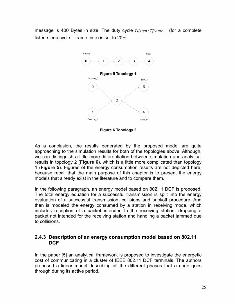
message is 400 Bytes in size. The duty cycle (for a complete listen-sleep cycle = frame time) is set to 20%.

Figure 5 Topology 1

Figure 6 Topology 2

As a conclusion, the results generated by the proposed model are quite approaching to the simulation results for both of the topologies above. Although, we can distinguish a little more differentiation between simulation and analytical results in topology 2 (Figure 6), which is a little more complicated than topology 1 (Figure 5). Figures of the energy consumption results are not depicted here, because recall that the main purpose of this chapter is to present the energy models that already exist in the literature and to compare them.

In the following paragraph, an energy model based on 802.11 DCF is proposed. The total energy equation for a successful transmission is split into the energy evaluation of a successful transmission, collisions and backoff procedure. And then is modeled the energy consumed by a station in receiving mode, which includes reception of a packet intended to the receiving station, dropping a packet not intended for the receiving station and handling a packet jammed due to collisions.

2.4.3 Description of an energy consumption model based on 802.11 DCF

In the paper [5] an analytical framework is proposed to investigate the energetic cost of communicating in a cluster of IEEE 802.11 DCF terminals. The authors proposed a linear model describing all the different phases that a node goes through during its active period.

26

This network model is a cluster of n IEEE 802.11 terminals using the Distributed Coordination Function (DCF), which is the native ad–hoc mode used in most commercial wireless devices. Such n terminals share the same radio channel and there is no hidden or exposed node. It is assumed that the cluster is under heavy traffic conditions, so that at each instant we have exactly n active packets: under this assumption, in fact, each node in the cluster is either performing the exponential backoff procedure or transmitting a packet.

In this model the advantage is that it has been taken into account collision delay, backoff delay, carrier sensing time, as well as it does the differentiation between receiving and sensing power and also introduces low power consumption mode.

More precisely it is denoted:: power to transmit a packet: power to decode a signal

: power to sense the media

: low power consumption

Energy Model-Transmitting power

The overall energy required for a node to transmit a packet with success is .

Where it is assumed that:: energy required for a successful transmission

: energy wasted into collisions

: the overall energy spent due to the backoff procedure

It is assumed for simplicity’s sake, that SIFS intervals are spent entirely to switch from receiving to transmitting mode and vise versa, with no additional power consumption.

Energy required for a successful transmission ,

for basic access mode; ,

for CTS/RTS mode.

27

Where: , , and are the duration of a data packets, ACK packets,

RTS and CTS packets.

Energy wasted into collisions ,

for basic access mode, ,

for CTS/RTS mode.

This means that the transmitter sends the whole packet and senses the media for ACK or CTS, but doesn’t receive an answer because the packet has been collided. The term corresponds to the EIFS (Extended Inder Frame

Space) interval.

In this paper is also considered the : the overall energy spent due to the

backoff procedure, and also it follows a linear model for the energy consumption, as well as statistics, but here we only introduce the energy model for simplicity reasons.

Energy Model-Receiving power

We distinguish three major cases for the energy consumed by a station in receiving mode: reception of a packet intended to the receiving station, dropping a packet not intended for the receiving station and handling a packet jammed due to collisions.

Respectively, energy for receiving a packet ,

for basic access mode,

, ,

for CTS/RTS mode.

Energy for dropping a packet not intended for the receiving station

for basic access mode,

for CTS/RTS mode.

28

where

for the RTS/CTS mode,

in the basic access mode and is the duration of the packet header.

Energy for handling a packet jammed due to collisions

for basic access mode,

for CTS/RTS mode.

where is the duration of a collision in basic access mode, with the assumption

a station stops decoding after detecting a jammed header. In CTS/RTS mode, collisions involve RTS packets only.

To conclude this case study, some interesting remarks were come out. In particular, for some packet lengths, transmitting with the RTS/CTS mode at a lower throughput than the basic access mode permits net energy savings. Also, using the NAV information and switching off receivers under discarding traffic, turns out to extend significantly the lifetime of stations. But, the advantage of such a technique disappears as soon as the power consumption in the low–power mode exceeds ½ of the receiving power.

In the next paragraph, an energy model based on 802.11e is proposed which includes two functions. The first one is the Hybrid Coordination Function (HCF) that is the modification of PCF function. The second is the Enhanced Distributed Control Function (EDCF) that adapts the DCF function to support QoS.

2.4.4 Description of an energy model based on 802.11e with HCF and EDCF

In the paper [6] a linear energy consumption model is proposed describing all energy contributions in IEEE 802.11e networks. The energy model is based on the “Mathematical Analysis of IEEE 802.11 Energy Efficiency” [5] as it had been

29

described above. The only advantage is that here was taken into account the more recent 802.11e standard with QoS support.

In particular, this standard includes two functions. The first one is the Hybrid Coordination Function (HCF) that is the modification of PCF function. The second is the Enhanced Distributed Control Function (EDCF) that adapts the DCF function to support QoS. EDCF defines 4 Access Categories (ACs). Each AC represents service having specific parameters. As a maximum, stations support 8 User Priority (UPs), called Traffic Categories (TCs). To each AC corresponds one or more TC. For example, access category 0 , has user priority 0,1,2 and corresponds to best effort designation.

Energy Model

We assume that there are K ACs in the network with different QoS requirements. All stations with traffic class k use the same parameters to access the channel,

, , .

Therefore, for each ACk, the total energy required to transmit a packet with success is

Also for the receiving operation the same as in [5] , but taking k as parameter:, , .

In the following section (2.4.5) is described an energy consumption model in a Single Hop IEEE 802.11 Ad Hoc network, under ideal conditions.

2.4.5 Description of an energy consumption model in Single Hop IEEE 802.11 Ad Hoc network

In the article [7] has been reported a detailed description of energy consumption in saturated IEEE 802.11 single-hop ad hoc networks, under ideal conditions. Considering the energy model, in the active management mechanism, a mode can be in transmit, receive or idle radio mode. It is a fact that when a node senses the channel in order to send a data frame, it becomes a potential receiver of the other node’s transmissions. The advantageous point here is that there are considered the IFS times in two modes: active and passive mode. On the other hand it is not considered the SLEEP mode.

30

Service Time Model

In the model, the channel state can be divided into three exclusive events,

(idle channel), (collision), (successful transmission). These events

dominate the behavior of the binary exponential backoff algorithm in 802.11. The average service time is divided in two parts: the time a node spends in backoff ( ), and the time a node needs to send a frame successfully ( ).

For the average backoff time ,

where .

is the minimum contention window size specified for the backoff operation,

is the standard-defined maximum power used to set up the maximum contention window size, is the conditional probability of a successful handshake, and , (where , , and

are the channel state probabilities that a node perceives during its

backoff operation, with , , and being their corresponding average time

duration).As a result the average service time (T) is

,

Where, Ts is the average service time to be transmitted the packet successfully. Also, nodes communicate through the four-handshake mechanism based on the “CTS-RTS” mechanism. So we have

where (request to send), (clear to send), and (acknowledgement) are the times to transmit each of the control frames, and are the standard-defined time intervals corresponding to the short

31

interframe space and the distributed interframe space, is the propagation delay, H is the time to transmit the packet header, and is the time to

transmit the average payload size.

Energy Consumption Model

In order to calculate the energy consumption of the system, under saturation conditions, we consider three main channel states: successful transmission, collision and idle channel states.

In the successful transmission we can point two occasions: the successful transmission between any two nodes in network and the successful transmission having the node itself as the target receiver. In the first one, the node in backoff overhears an updates its network allocation vector (NAV) and then freezes its backoff time counter for the duration of someone’s else four-way handshake.In the second occasion, the node itself is the recipient of the transfer, so it has to receive from the sender and send back to him the .

In the collision channel state is either overhearing ( an unsuccessful transmission ) or being the target of the transmission ( failed transmission ).Also, it is too important to be referred that energy is consumed while overhearing and receiving modes, during the and after overhearing or receiving failed handshakes.

In the idle channel state, the node senses the channel and decreases its backoff counter each time no activity is detected for the duration of a time slot. When this counter becomes zero, the node will be ready to send its data frame.

These three states cover the times during the backoff stage of the node and before it attempts the handshake. At the end of its backoff, the node attempts to establish a handshake with the receiver. If the backoff is finished and the handshake failed, the node needs to remake backoff and repeats the same process, until it finally succeed establishing handshake and before reaches to the maximum number of allowed retransmissions.

In a successful four-way handshake, during the Ts, the node transmits an and a frame and receives a and an from the receiver. Then it stays idle during the and the propagation delay . A basic point is that according to experimental results, reported by Feeney, The energy consumption of overhearing a frame , staying idle, or sensing the channel are only marginally different from the energy consumption of receiving a frame.

32

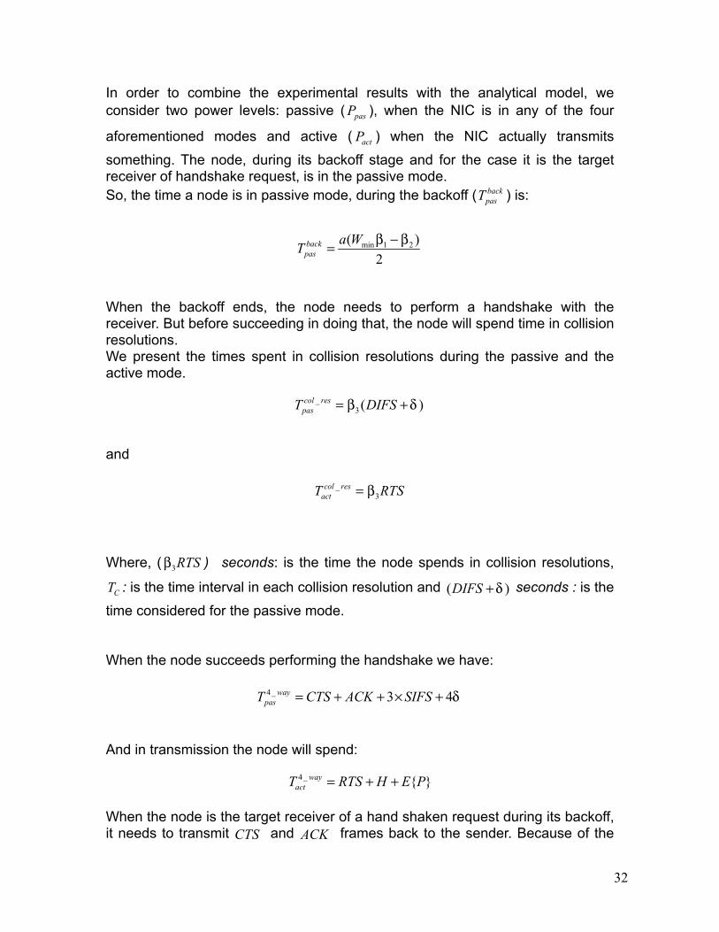
In order to combine the experimental results with the analytical model, we consider two power levels: passive ( ), when the NIC is in any of the four

aforementioned modes and active ( ) when the NIC actually transmits

something. The node, during its backoff stage and for the case it is the target receiver of handshake request, is in the passive mode.So, the time a node is in passive mode, during the backoff ( ) is:

When the backoff ends, the node needs to perform a handshake with the receiver. But before succeeding in doing that, the node will spend time in collision resolutions.We present the times spent in collision resolutions during the passive and the active mode.

and

Where, ( ) seconds: is the time the node spends in collision resolutions,

: is the time interval in each collision resolution and seconds : is the

time considered for the passive mode.

When the node succeeds performing the handshake we have:

And in transmission the node will spend:

When the node is the target receiver of a hand shaken request during its backoff, it needs to transmit and frames back to the sender. Because of the

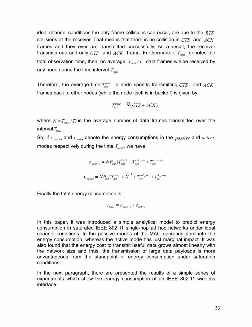
33

ideal channel conditions the only frame collisions can occur, are due to the collisions at the receiver. That means that there is no collision in and frames and they ever are transmitted successfully. As a result, the receiver transmits one and only and frame. Furthermore, if denotes the

total observation time, then, on average, data frames will be received by

any node during the time interval .

Therefore, the average time a node spends transmitting and

frames back to other nodes (while the node itself is in backoff) is given by

where is the average number of data frames transmitted over the

interval .

So, if and denote the energy consumptions in the and

modes respectively during the time , we have

Finally the total energy consumption is:

In this paper, it was introduced a simple analytical model to predict energy consumption in saturated IEEE 802.11 single-hop ad hoc networks under ideal channel conditions. In the passive modes of the MAC operation dominate the energy consumption, whereas the active mode has just marginal impact. It was also found that the energy cost to transmit useful data grows almost linearly with the network size and thus, the transmission of large data payloads is more advantageous from the standpoint of energy consumption under saturation conditions.

In the next paragraph, there are presented the results of a simple series of experiments which show the energy consumption of an IEEE 802.11 wireless interface.

34

2.4.6 Description of an energy consumption model of a Wireless Network Interface in an Ad Hoc Networking Environment

The purpose of the article [8] is to calculate the energy consumption in an IEEE 802.11 wireless network interface operating in an ad hoc networking environment and it is succeeded through a series of experiments which obtained detailed measurements. It takes into account the RTS-CTS but does not consider IFS times, link-layer fragmentation and energy consumption in the unsuccessful attempts of acquiring the channel and when messages are lost due to collision.

Here there are considered two modes of operation, the Base Station mode ( ) and the Ad Hoc mode .The first one has to be ever in a transmission range one or more base stations which are responsible for buffering and forwarding traffic between hosts. In Ad Hoc mode, all nodes in transmission range communicate with other nodes directly. Network interfaces in this mode, do not sleep and they have constant power consumption, the cost of listening to the wireless channel.

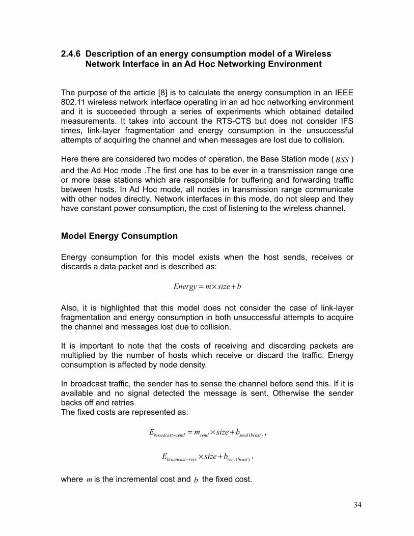
Model Energy Consumption

Energy consumption for this model exists when the host sends, receives or discards a data packet and is described as:

Also, it is highlighted that this model does not consider the case of link-layer fragmentation and energy consumption in both unsuccessful attempts to acquire the channel and messages lost due to collision.

It is important to note that the costs of receiving and discarding packets are multiplied by the number of hosts which receive or discard the traffic. Energy consumption is affected by node density.

In broadcast traffic, the sender has to sense the channel before send this. If it is available and no signal detected the message is sent. Otherwise the sender backs off and retries.The fixed costs are represented as:

,

,

where is the incremental cost and the fixed cost.

35

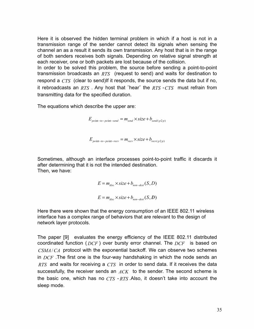
Here it is observed the hidden terminal problem in which if a host is not in a transmission range of the sender cannot detect its signals when sensing the channel an as a result it sends its own transmission. Any host that is in the range of both senders receives both signals. Depending on relative signal strength at each receiver, one or both packets are lost because of the collision.In order to be solved this problem, the source before sending a point-to-point transmission broadcasts an (request to send) and waits for destination to respond a (clear to send)If it responds, the source sends the data but if no, it rebroadcasts an . Any host that ¨hear¨ the - must refrain from transmitting data for the specified duration.

The equations which describe the upper are:

Sometimes, although an interface processes point-to-point traffic it discards it after determining that it is not the intended destination.Then, we have:

Here there were shown that the energy consumption of an IEEE 802.11 wireless interface has a complex range of behaviors that are relevant to the design of network layer protocols.

The paper [9] evaluates the energy efficiency of the IEEE 802.11 distributed coordinated function ( ) over bursty error channel. The is based on

protocol with the exponential backoff. We can observe two schemes in .The first one is the four-way handshaking in which the node sends an

and waits for receiving a in order to send data. If it receives the data successfully, the receiver sends an to the sender. The second scheme is the basic one, which has no - .Also, it doesn’t take into account the sleep mode.

36

System Model

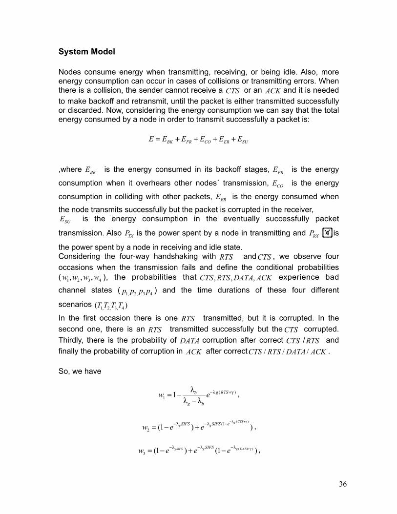
Nodes consume energy when transmitting, receiving, or being idle. Also, more energy consumption can occur in cases of collisions or transmitting errors. When there is a collision, the sender cannot receive a or an and it is needed to make backoff and retransmit, until the packet is either transmitted successfully or discarded. Now, considering the energy consumption we can say that the total energy consumed by a node in order to transmit successfully a packet is:

,where is the energy consumed in its backoff stages, is the energy

consumption when it overhears other nodes´ transmission, is the energy

consumption in colliding with other packets, is the energy consumed when

the node transmits successfully but the packet is corrupted in the receiver, is the energy consumption in the eventually successfully packet

transmission. Also is the power spent by a node in transmitting and is

the power spent by a node in receiving and idle state.Considering the four-way handshaking with and , we observe four occasions when the transmission fails and define the conditional probabilities ( ), the probabilities that experience bad

channel states ( ) and the time durations of these four different

scenarios

In the first occasion there is one transmitted, but it is corrupted. In the second one, there is an transmitted successfully but the corrupted. Thirdly, there is the probability of corruption after correct / and finally the probability of corruption in after correct .

So, we have

,

,

,

37

.

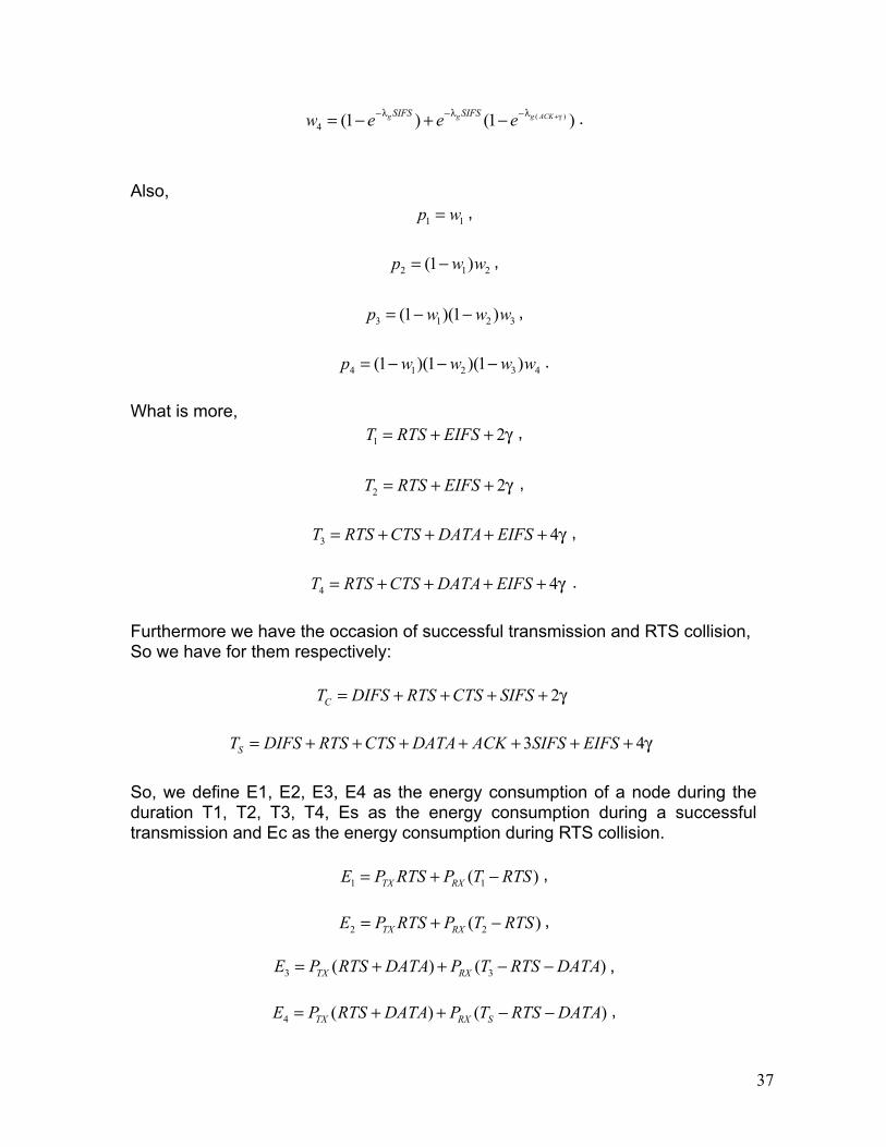
Also, ,

,

,

.

What is more, ,

,

,

.

Furthermore we have the occasion of successful transmission and RTS collision,So we have for them respectively:

So, we define E1, E2, E3, E4 as the energy consumption of a node during the duration T1, T2, T3, T4, Es as the energy consumption during a successful transmission and Ec as the energy consumption during RTS collision.

,

,

,

,

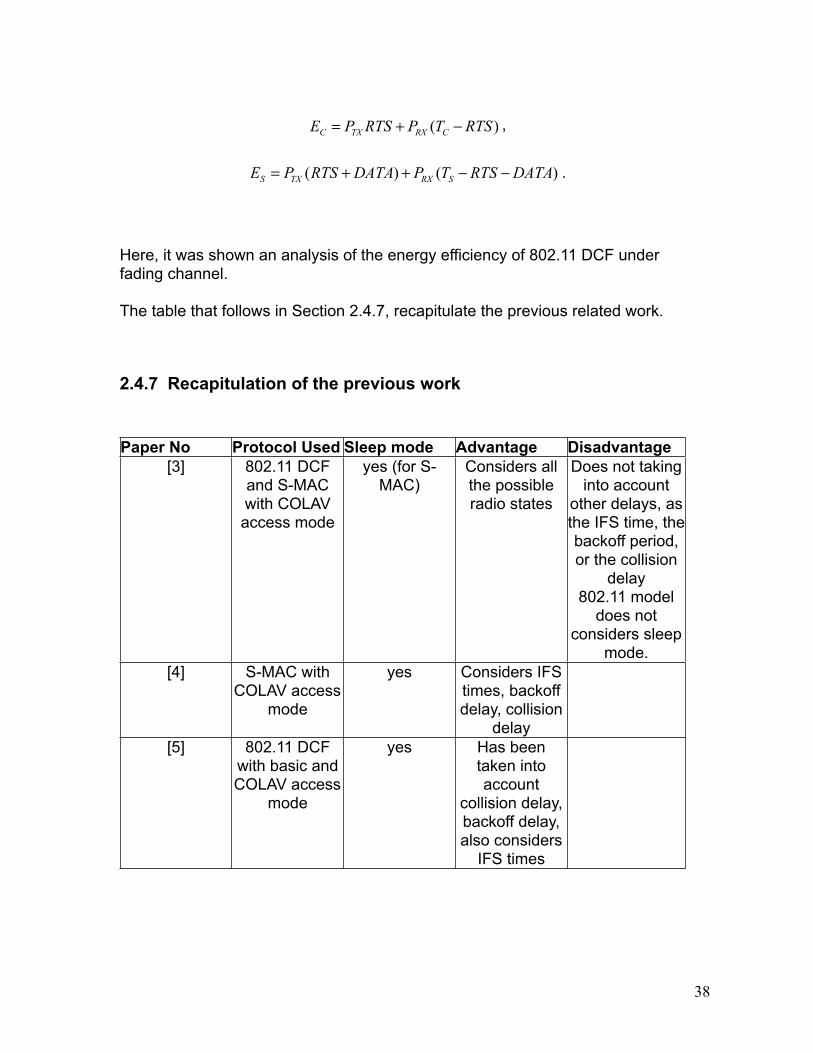
38

,

.

Here, it was shown an analysis of the energy efficiency of 802.11 DCF under fading channel.

The table that follows in Section 2.4.7, recapitulate the previous related work.

2.4.7 Recapitulation of the previous work

Paper No Protocol Used Sleep mode Advantage Disadvantage[3] 802.11 DCF

and S-MAC with COLAV access mode

yes (for S-MAC)

Considers all the possible radio states

Does not taking into account

other delays, as the IFS time, the backoff period, or the collision

delay802.11 model

does not considers sleep

mode. [4] S-MAC with

COLAV access mode

yes Considers IFS times, backoff delay, collision

delay[5] 802.11 DCF

with basic and COLAV access

mode

yes Has been taken into account

collision delay, backoff delay, also considers

IFS times

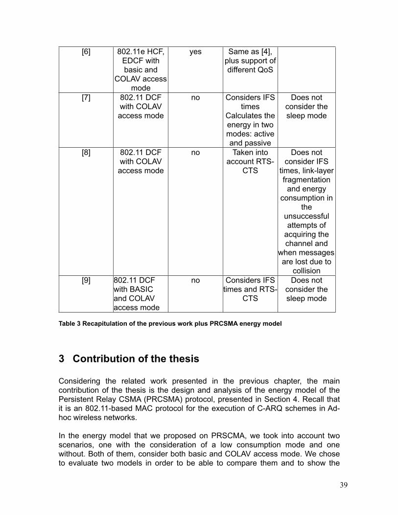
39

[6] 802.11e HCF, EDCF with basic and

COLAV access mode

yes Same as [4], plus support of different QoS

[7] 802.11 DCF with COLAV access mode

no Considers IFS times

Calculates the energy in two modes: active and passive

Does not consider the sleep mode

[8] 802.11 DCF with COLAV access mode

no Taken into account RTS-

CTS

Does not consider IFS

times, link-layer fragmentation and energy

consumption in the

unsuccessful attempts of

acquiring the channel and

when messages are lost due to

collision[9] 802.11 DCF

with BASIC and COLAV access mode

no Considers IFS times and RTS-

CTS

Does not consider the sleep mode

Table 3 Recapitulation of the previous work plus PRCSMA energy model

3 Contribution of the thesis

Considering the related work presented in the previous chapter, the main contribution of the thesis is the design and analysis of the energy model of the Persistent Relay CSMA (PRCSMA) protocol, presented in Section 4. Recall that it is an 802.11-based MAC protocol for the execution of C-ARQ schemes in Ad-hoc wireless networks.

In the energy model that we proposed on PRSCMA, we took into account two scenarios, one with the consideration of a low consumption mode and one without. Both of them, consider both basic and COLAV access mode. We chose to evaluate two models in order to be able to compare them and to show the

40

benefits of a low consumption mode in the total energy consumption. Also, we considered all possible radio states (transmit, receive and idle). What is more, we took into account backoff delay, collision delay and IFS times, in order to have more accurate results.

Also, PRCSMA protocol is also compared from the energy efficiency point of view to an ideal perfect scheduling system. Ideal means that there is no contention and accordingly no idle or collision slots. This comparison explicitly evaluates the energy consumption overhead generated by an actual MAC protocol and demonstrates that its overhead must not be neglected in order to evaluate the real performance of any C-ARQ scheme.

What is more, PRCSMA protocol is compared in terms of energy efficiency to two non-cooperative scenarios; one that takes into account the energy consumption only of the source and the destination and another that takes into account the energy consumption of the whole network. This comparison shows us which of PRCSMA and the two non-cooperative scenarios are more energy efficient under different parameters and which is more worth to use in each case.

Besides that, the energy fairness of the system model has been introduced, in order to find out if all the relays consume the same amount of energy under PRCSMA, and that means to have the same battery lifetime which is very important for wireless devices.

In the following chapter, is presented the framework of the thesis, where the C-ARQ and the PRSCMA protocol are analysed.

4 Framework

In this chapter, the C-ARQ (Cooperative ARQ), the IEEE 802.11 protocol for Ad-hoc networks and the PRSCMA protocol are analysed in Sections 4.1 and 4.2, respectively.

4.1 Cooperative ARQ Scheme in Wireless Networks

Traditionally, ARQ (Automatic Retransmission/Repeat Request) schemes have been used in communication networks to guarantee the reliable delivery of data packets. Upon the reception of a packet with errors, retransmissions are requested from the source until either the packet can be properly decoded or it is discarded for the benefit of the backlogged data. Error Detection (ED) information

41

is usually attached to the data packets so that the intended destination can learn whether a packet has been received with errors or not. Typically, this ED information gets the form of a CRC attached to the overhead (either to the header or to the tail) of data packets. In hybrid ARQ schemes, Forward Error Correction (FEC) information is also attached to the overhead of the packets in order to reduce the probability of error occurrence. According to the retransmitted information, ARQ schemes can be classified as:1) Type I, if retransmissions are exact copies of the failed packet.2) Type II, if there is incremental redundancy added to the retransmissions.

The focus in this part of the thesis is on Cooperative ARQ (C-ARQ) schemes. C-ARQ is a very active research topic today and C-ARQ schemes constitute a practical way of executing cooperation in wireless networks with already existing equipment and taking into account the aforementioned market figures. C-ARQ schemes can be considered as a kind of cooperative schemes that exploit feedback from the receiver. In C-ARQ, cooperation is only requested when actually needed, and thus the efficiency of the network can be improved. What is more, the independent transmission paths by the relays provide diversity. C-ARQ schemes can provide spatial diversity and attain higher reliability of the transmissions, higher transmission rates, lower transmission delays, more efficient energy consumption, or extended coverage, among other possibilities.[2]

In short, the idea of C-ARQ is to make use of the broadcast nature of the wireless channel in the following manner: any transmission can be received by not only the intended destination of the transmission, but also by any of the stations in the transmission range of the transmitter. In case of a transmission error, a retransmission can be requested from any (or some) of the stations which overheard the original transmission, which can act as spontaneous helpers (or relays). This can be done by broadcasting a Call for Cooperation (CFC) packet. [2]

The Relays are intermediate stations who help the destination station to receive the information packet, even if the latter is out of range of the source station, by retransmitting the packet (cooperative packet). More precisely, they keep a copy of any received data packet (regardless of its destination address) until it is acknowledged (positively or negatively) by the destination. This packet is discarded whenever the destination successfully decodes the original packet. The copy retained by the stations might be stored at each station data buffer.

Eventually, the destination might either receive a correct copy of the original packet from a relay or may be able to properly combine the different retransmissions from the relays to successfully decode the original packet. Otherwise, if the destination is not able to recover the data packet after some predefined time (cooperation timeout), it is discarded. In any of the two cases, the cooperation phase is finished.

42

At this point, we have to state that in our model on PRCSMA, we assumed that the relays send exact copies of the failed packet, so, with the first correct packet cooperation phase is ended and the destination sends the ACK.

Put in mind that the relays that are closer to the destination than the transmitter can retransmit the information faster, with a higher transmission rate. As a result, there is lower cost of channel time use.

Recall that the active relays attempt orthogonally in time (Time Division Multiple Access -TDMA), frequency (Frequency Division Multiple Access -FDMA or Orthogonal Frequency-Division Multiple Access -OFDMA), or code (Code division multiple access -CDMA), to retransmit a copy of the original packet to assist in the failed transmission.

In particular, the focus in this thesis is on time-orthogonal C-ARQ schemes, which are feasible to be implemented with already existing off-the-shelf equipment and there is no need for synchronization among the relays because they retransmit one after another in time. More precisely, by slightly modifying the wireless controller (or driver), existing wireless cards could implement a C-ARQ scheme. The emphasis is on the design and analysis of novel MAC protocols to deal with the unique characteristics of the contention process that takes place among the active relays within a cooperation phase. Note that in the considered C-ARQ (PRCSMA) schemes, upon the initialization of the cooperation phase, the network has the three following unique characteristics:

1) The spontaneous “sub-network” formed by the active relays is ad hoc and thus there is no infrastructure responsible for managing the access to the channel.2) This sub-network formed by the active relays surrounding the node calling for cooperation is suddenly (sharply) set into saturation conditions whenever the cooperation phase is initiated. Upon the transmission of a CFC packet, all the active relays have a data packet ready to transmit in order to assist the failed transmission.

Therefore, heavy contention comes up in a previously idle network. These characteristics determine the design of PRCSMA within the context of C-ARQ schemes in wireless networks.

4.2 PRCSMA (Persistent Relay Carrier Sensing Multiple Access)

Considering the drawbacks of the standard MAC protocol for its use in the C-ARQ scheme, the Persistent Relay Carrier Sensing Multiple Access (PRCSMA) [2] has been proposed as an extension and adaptation of the IEEE 802.11 MAC protocol to meet the requirements of the C-ARQ scheme.

43

More precisely, the IEEE 802.11 MAC protocol has not been specifically designed to be executed in C-ARQ schemes. It provides fair long-term access and runs in stable conditions over WLANs (with limited number of active users and under not very heavy traffic conditions) [17]. However, if 802.11 was used in a C-ARQ scheme, it would provide a highly inefficient access operation. Fist, the virtual carrier sensing mechanism should not be used, because otherwise, stations are oblivious to transmissions not directed to them and thus cooperation cannot be executed. In this way, upon the transmission of a CFC, all the active relays would attempt to transmit after a DIFS period. This would result in an unavoidable collision. All the active relays would then double up their contention window, which would lead to an unnecessary increase of the transmission delay. Therefore, these are the reasons that make 802.11 insufficient for C-ARQ schemes and bring the need of designing a new protocol as PRCSMA.

To begin with, PRCSMA works as follows: all the stations must listen to every ongoing transmission in order to be able to cooperate if required. In addition, they should keep a copy of any received data packet (regardless of its destination address) until it is acknowledged by the destination station. It is important to note that the term destination station will be used denote the next-hop destination of a packet.

Whenever a data packet is received with errors at the destination station, a cooperation phase can be initiated by broadcasting a claim for cooperation (CFC) message in the form of a control packet after sensing the channel idle for an SIFS period. Regular data transmissions in IEEE 802.11 are done after a longer silence period (DIFS), and thus cooperation phases are given priority over regular data traffic. We also can say that the destination station acts like a master and the relays as slaves. A subset of the stations which overheard both the original transmission from the source and the CFC from the destination, become active relays or helpers. This subset is referred to as the active relay set and the data packets retransmitted by the relays will be referred to as cooperative packets.

During each cooperation phase all the relays attempt to transmit a packet and, therefore, every station is either transmitting or in backoff. The main assumption for the proposed model is that the relays use a constant CW length, i.e., they do not double up the CW upon collision or erroneous transmission. Therefore, the CW is selected randomly within the interval [0,W]. The main reason for this assumption is that the results for a variable CW can be accurately approximated by those for a constant CW, based on [17]. In addition, recall that in the basic access mode of PRCSMA there is no ACK associated to each transmission, and thus collision detection cannot be performed by the relays unless the COLAV access method is executed.

It is worth recalling that the retransmitted copy may be simply an amplified version of the original received packet at each relay, a compressed version of the

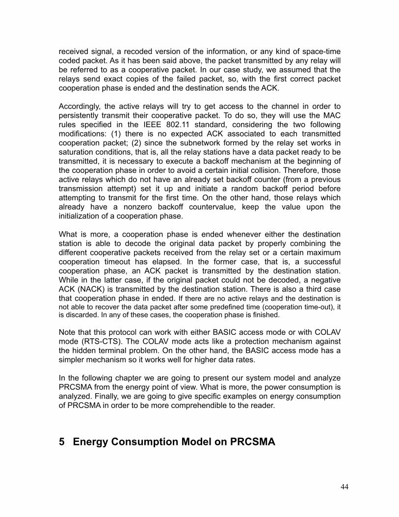
44

received signal, a recoded version of the information, or any kind of space-time coded packet. As it has been said above, the packet transmitted by any relay will be referred to as a cooperative packet. In our case study, we assumed that the relays send exact copies of the failed packet, so, with the first correct packet cooperation phase is ended and the destination sends the ACK.

Accordingly, the active relays will try to get access to the channel in order to persistently transmit their cooperative packet. To do so, they will use the MAC rules specified in the IEEE 802.11 standard, considering the two following modifications: (1) there is no expected ACK associated to each transmitted cooperation packet; (2) since the subnetwork formed by the relay set works in saturation conditions, that is, all the relay stations have a data packet ready to be transmitted, it is necessary to execute a backoff mechanism at the beginning of the cooperation phase in order to avoid a certain initial collision. Therefore, those active relays which do not have an already set backoff counter (from a previous transmission attempt) set it up and initiate a random backoff period before attempting to transmit for the first time. On the other hand, those relays which already have a nonzero backoff countervalue, keep the value upon the initialization of a cooperation phase.

What is more, a cooperation phase is ended whenever either the destination station is able to decode the original data packet by properly combining the different cooperative packets received from the relay set or a certain maximum cooperation timeout has elapsed. In the former case, that is, a successful cooperation phase, an ACK packet is transmitted by the destination station. While in the latter case, if the original packet could not be decoded, a negative ACK (NACK) is transmitted by the destination station. There is also a third case that cooperation phase in ended. If there are no active relays and the destination is not able to recover the data packet after some predefined time (cooperation time-out), it is discarded. In any of these cases, the cooperation phase is finished.

Note that this protocol can work with either BASIC access mode or with COLAV mode (RTS-CTS). The COLAV mode acts like a protection mechanism against the hidden terminal problem. On the other hand, the BASIC access mode has a simpler mechanism so it works well for higher data rates.

In the following chapter we are going to present our system model and analyze PRCSMA from the energy point of view. What is more, the power consumption is analyzed. Finally, we are going to give specific examples on energy consumption of PRCSMA in order to be more comprehendible to the reader.

5 Energy Consumption Model on PRCSMA

45

5.1 System Model

The topology used is composed of a source, a destination and a number of nodes n (potential relays), that a subset of these will become active relays to assist in a failed transmission.

These stations then can overhear the transmissions from the source to the destination. Due to the propagation losses and the channel fading, the average SNR in the link from source to destination is assumed to be low. Therefore, the available effective transmission rate between source and destination is also low, at least compared to the ones available between the stations close to the destination and the destination itself. For this reason, retransmissions from the source are costly in terms of channel usage and a C-ARQ scheme can help in improving the performance of the network and extending the coverage of the source to be able to intercommunicate with distant stations. It is considered that the relays execute a “Decode and Forward” scheme to retransmit when required. Thus, the relays transmit recoded copies of the original message. The recoding process can be done in the basis of repeating the original codification. Also, a No Line-Of-Sight (NLOS) block-fading Rayleigh channel is considered. In particular, block-fading means that the channel quality is assumed to remain constant at least for the transmission of a whole single data packet.

The transmission rate between the source and any destination station is selected according to the channel quality of the corresponding link. The set of available transmission rates is discrete, as in most practical wireless communication systems.

It is assumed that all the potential relays are homogeneously distributed around the destination station. An abstract model of this scenario is represented in Figure 7.

Figure 7 System Model

46

Once the source selects one specific destination station (D), the other n stations close to D become spontaneous potential relays. The destination station transmits a CFC packet only when a data packet from the destination is received with errors. The particular case wherein those stations which successfully (without errors) receive both the original data packet from the source and the CFC from the destination station become active relays is considered. In case that any of the potential relays become active relays, then we have a cooperation timeout, which means that the source waits so long as the maximum contention window is defined.

It is assumed that the channel quality between the relays and the destination station is such that transmissions in the control plane are error-free, and thus the CFC is received without errors by all the potential relays (recall that control packets are transmitted at the most robust coding scheme and are very short in length compared to data packets).

On the other hand, the relays apply a ‘Decode and Forward’ scheme, i.e., they transmit correct copies of the original packet, and thus the average number of transmissions from the relays required to decode the packet at destination depends on the .

5.2 Energy Consumption Model

Considering all the previous work, we now present our energy consumption model in PRCSMA. First of all, we consider that there are four radio operation modes:

1. the transmitting mode, when radio is transmitting data packets or control frames,

2. the receiving mode, when radio is receiving data or control frames effectively,

3. the idle mode, when radio is sensing the media, and4. the sleepping mode, when radio is in low power, and it is not able to

receive or transmit. The power associated to each mode is , power to transmit a packet, ,

power to receive a packet, , power to sense the media and , low power

consumption respectively.

The energy consumption is calculated as

,

where, is the power and the time.

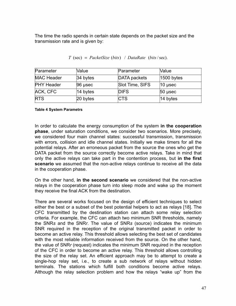
47

The time the radio spends in certain state depends on the packet size and the transmission rate and is given by:

Parameter Value Parameter ValueMAC Header 34 bytes DATA packets 1500 bytesPHY Header 96 µsec Slot Time, SIFS 10 µsecACK, CFC 14 bytes DIFS 50 µsecRTS 20 bytes CTS 14 bytes

Table 4 System Parametrs

In order to calculate the energy consumption of the system in the cooperation phase, under saturation conditions, we consider two scenarios. More precisely, we considered four main channel states: successful transmission, transmission with errors, collision and idle channel states. Initially we make timers for all the potential relays. After an erroneous packet from the source the ones who get the DATA packet from the source correctly become active relays. Take in mind that only the active relays can take part in the contention process, but in the first scenario we assumed that the non-active relays continue to receive all the data in the cooperation phase.

On the other hand, in the second scenario we considered that the non-active relays in the cooperation phase turn into sleep mode and wake up the moment they receive the final ACK from the destination.

There are several works focused on the design of efficient techniques to select either the best or a subset of the best potential helpers to act as relays [18]. The CFC transmitted by the destination station can attach some relay selection criteria. For example, the CFC can attach two minimum SNR thresholds, namely the SNRs and the SNRr. The value of SNRs (source) indicates the minimum SNR required in the reception of the original transmitted packet in order to become an active relay. This threshold allows selecting the best set of candidates with the most reliable information received from the source. On the other hand, the value of SNRr (request) indicates the minimum SNR required in the reception of the CFC in order to become an active relay. This threshold allows controlling the size of the relay set. An efficient approach may be to attempt to create a single-hop relay set, i.e., to create a sub network of relays without hidden terminals. The stations which fulfill both conditions become active relays. Although the relay selection problem and how the relays “wake up” from the

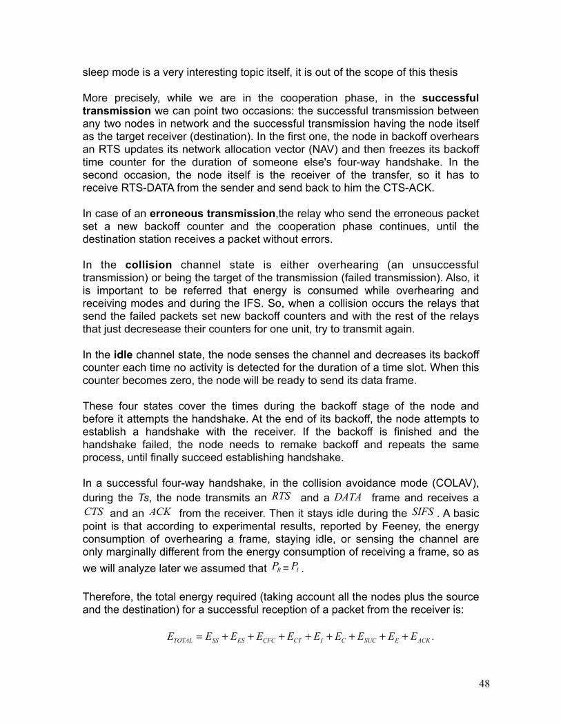
48

sleep mode is a very interesting topic itself, it is out of the scope of this thesis

More precisely, while we are in the cooperation phase, in the successful transmission we can point two occasions: the successful transmission between any two nodes in network and the successful transmission having the node itself as the target receiver (destination). In the first one, the node in backoff overhears an RTS updates its network allocation vector (NAV) and then freezes its backoff time counter for the duration of someone else's four-way handshake. In the second occasion, the node itself is the receiver of the transfer, so it has to receive RTS-DATA from the sender and send back to him the CTS-ACK.

In case of an erroneous transmission,the relay who send the erroneous packet set a new backoff counter and the cooperation phase continues, until the destination station receives a packet without errors.

In the collision channel state is either overhearing (an unsuccessful transmission) or being the target of the transmission (failed transmission). Also, it is important to be referred that energy is consumed while overhearing and receiving modes and during the IFS. So, when a collision occurs the relays that send the failed packets set new backoff counters and with the rest of the relays that just decresease their counters for one unit, try to transmit again.

In the idle channel state, the node senses the channel and decreases its backoff counter each time no activity is detected for the duration of a time slot. When this counter becomes zero, the node will be ready to send its data frame.

These four states cover the times during the backoff stage of the node and before it attempts the handshake. At the end of its backoff, the node attempts to establish a handshake with the receiver. If the backoff is finished and the handshake failed, the node needs to remake backoff and repeats the same process, until finally succeed establishing handshake.

In a successful four-way handshake, in the collision avoidance mode (COLAV), during the Ts, the node transmits an and a frame and receives a

and an from the receiver. Then it stays idle during the . A basic point is that according to experimental results, reported by Feeney, the energy consumption of overhearing a frame, staying idle, or sensing the channel are only marginally different from the energy consumption of receiving a frame, so as we will analyze later we assumed that = .

Therefore, the total energy required (taking account all the nodes plus the source and the destination) for a successful reception of a packet from the receiver is:

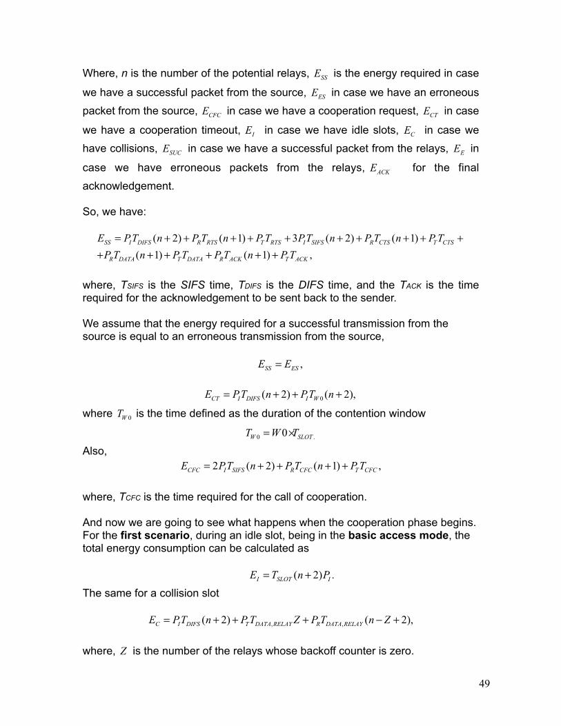
49

Where, n is the number of the potential relays, is the energy required in case

we have a successful packet from the source, in case we have an erroneous

packet from the source, in case we have a cooperation request, in case

we have a cooperation timeout, in case we have idle slots, in case we

have collisions, in case we have a successful packet from the relays, in

case we have erroneous packets from the relays, for the final

acknowledgement.

So, we have:

where, TSIFS is the SIFS time, TDIFS is the DIFS time, and the TACK is the time required for the acknowledgement to be sent back to the sender.

We assume that the energy required for a successful transmission from the source is equal to an erroneous transmission from the source,

where is the time defined as the duration of the contention window

Also,

where, TCFC is the time required for the call of cooperation.

And now we are going to see what happens when the cooperation phase begins.For the first scenario, during an idle slot, being in the basic access mode, the total energy consumption can be calculated as

The same for a collision slot

where, is the number of the relays whose backoff counter is zero.

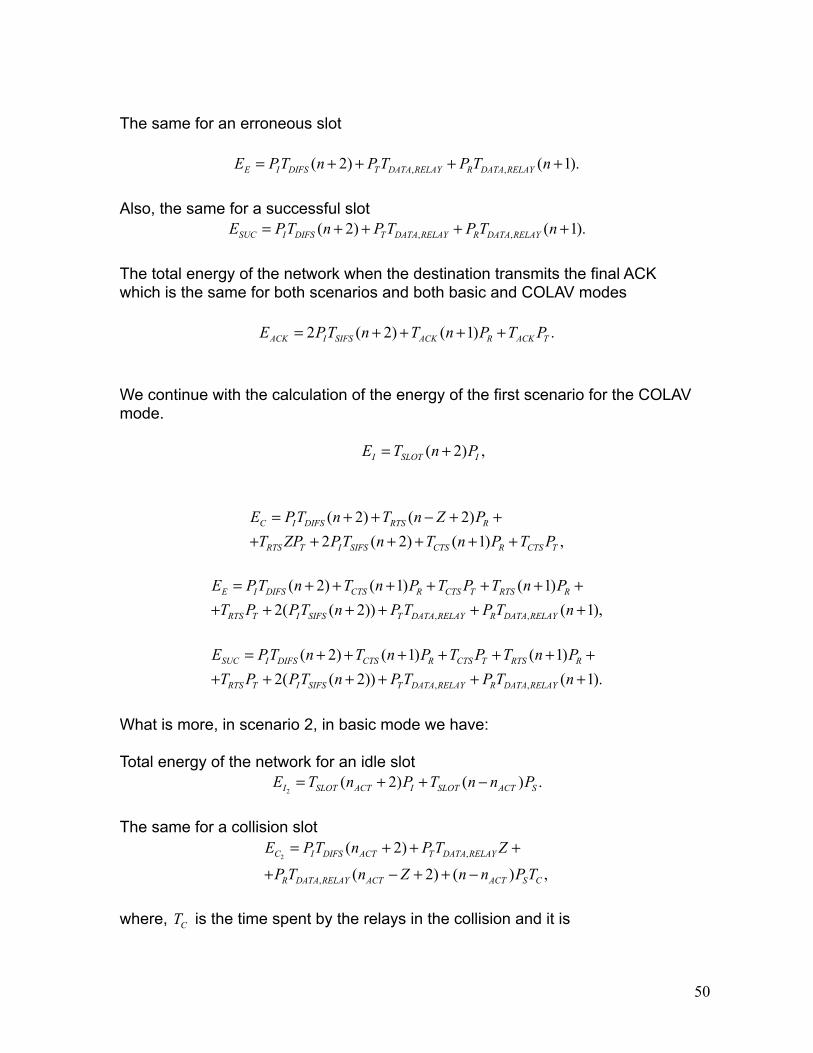
50

The same for an erroneous slot

Also, the same for a successful slot

The total energy of the network when the destination transmits the final ACK which is the same for both scenarios and both basic and COLAV modes

We continue with the calculation of the energy of the first scenario for the COLAV mode.

What is more, in scenario 2, in basic mode we have:

Total energy of the network for an idle slot

The same for a collision slot

where, is the time spent by the relays in the collision and it is

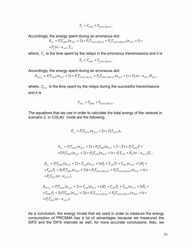
51

Accordingly, the energy spent during an erroneous slot

where, is the time spent by the relays in the erroneous transmissions and it is

Accordingly, the energy spent during an erroneous slot

where, is the time spent by the relays during the successful transmissions

and it is

The equations that we use in order to calculate the total energy of the network in scenario 2, in COLAV mode are the following:

As a conclusion, the energy model that we used in order to measure the energy consumption of PRCSMA has a lot of advantages because we measured the SIFS and the DIFS intervals as well, for more accurate conclusions. Also, we

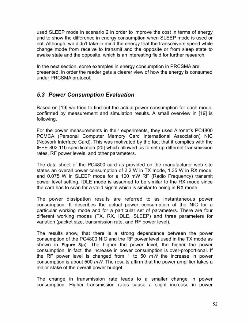
52

used SLEEP mode in scenario 2 in order to improve the cost in terms of energy and to show the difference in energy consumption when SLEEP mode is used or not. Although, we didn’t take in mind the energy that the transceivers spend while change mode from receive to transmit and the opposite or from sleep state to awake state and the opposite, which is an interesting field for further research.

In the next section, some examples in energy consumption in PRCSMA are presented, in order the reader gets a clearer view of how the energy is consumed under PRCSMA protocol.

5.3 Power Consumption Evaluation

Based on [19] we tried to find out the actual power consumption for each mode, confirmed by measurement and simulation results. A small overview in [19] is following.

For the power measurements in their experiments, they used Aironet’s PC4800 PCMCA (Personal Computer Memory Card International Association) NIC (Network Interface Card). This was motivated by the fact that it complies with the IEEE 802.11b specification [20] which allowed us to set up different transmission rates, RF power levels, and other parameters.

The data sheet of the PC4800 card as provided on the manufacturer web site states an overall power consumption of 2.2 W in TX mode, 1.35 W in RX mode, and 0.075 W in SLEEP mode for a 100 mW RF (Radio Frequency) transmit power level setting. IDLE mode is assumed to be similar to the RX mode since the card has to scan for a valid signal which is similar to being in RX mode.

The power dissipation results are referred to as instantaneous power consumption. It describes the actual power consumption of the NIC for a particular working mode and for a particular set of parameters. There are four different working modes (TX, RX, IDLE, SLEEP) and three parameters for variation (packet size, transmission rate, and RF power level).

The results show, that there is a strong dependence between the power consumption of the PC4800 NIC and the RF power level used in the TX mode as shown in Figure 8(a): The higher the power level, the higher the power consumption. In fact, the increase in power consumption is over-proportional. If the RF power level is changed from 1 to 50 mW the increase in power consumption is about 500 mW. The results affirm that the power amplifier takes a major stake of the overall power budget.

The change in transmission rate leads to a smaller change in power consumption. Higher transmission rates cause a slight increase in power

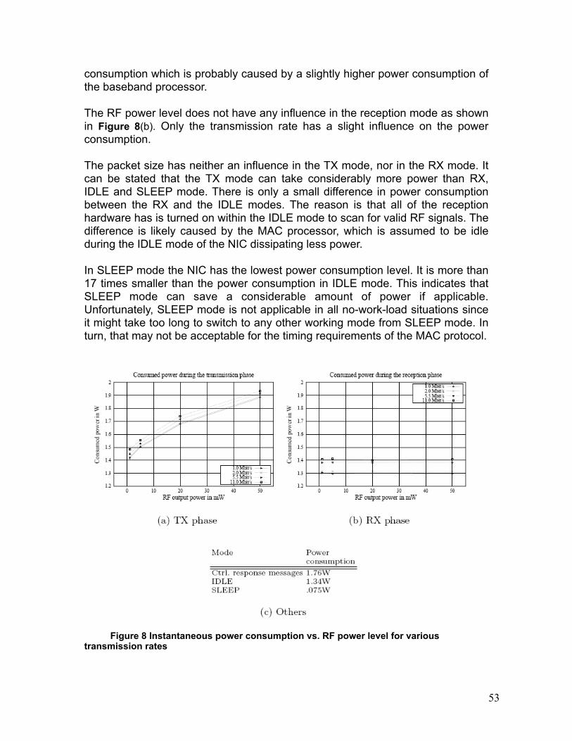
53

consumption which is probably caused by a slightly higher power consumption of the baseband processor.

The RF power level does not have any influence in the reception mode as shown in Figure 8(b). Only the transmission rate has a slight influence on the power consumption.

The packet size has neither an influence in the TX mode, nor in the RX mode. It can be stated that the TX mode can take considerably more power than RX, IDLE and SLEEP mode. There is only a small difference in power consumption between the RX and the IDLE modes. The reason is that all of the reception hardware has is turned on within the IDLE mode to scan for valid RF signals. The difference is likely caused by the MAC processor, which is assumed to be idle during the IDLE mode of the NIC dissipating less power.

In SLEEP mode the NIC has the lowest power consumption level. It is more than 17 times smaller than the power consumption in IDLE mode. This indicates that SLEEP mode can save a considerable amount of power if applicable. Unfortunately, SLEEP mode is not applicable in all no-work-load situations since it might take too long to switch to any other working mode from SLEEP mode. In turn, that may not be acceptable for the timing requirements of the MAC protocol.

Figure 8 Instantaneous power consumption vs. RF power level for various transmission rates

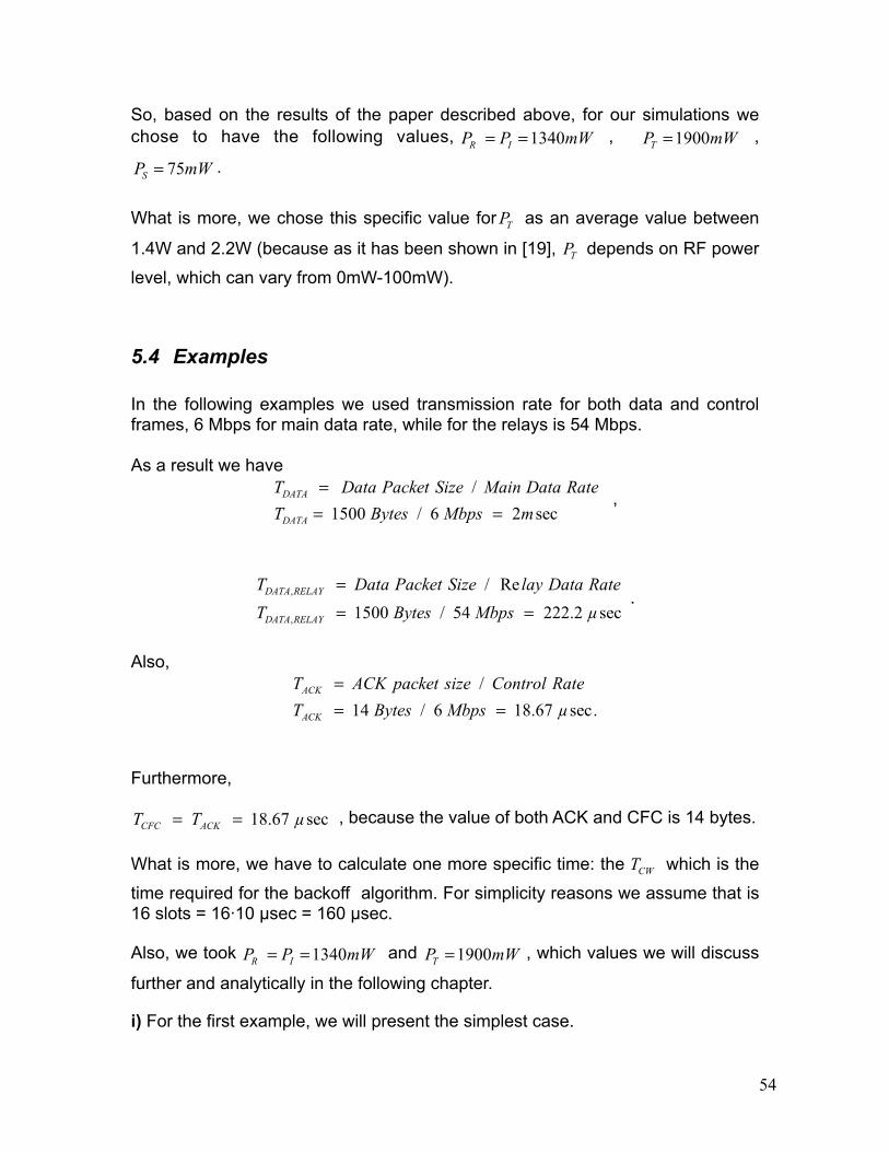
54

So, based on the results of the paper described above, for our simulations we chose to have the following values, , ,

.

What is more, we chose this specific value for as an average value between

1.4W and 2.2W (because as it has been shown in [19], depends on RF power

level, which can vary from 0mW-100mW).

5.4 Examples

In the following examples we used transmission rate for both data and control frames, 6 Mbps for main data rate, while for the relays is 54 Mbps.

As a result we have

,

.

Also,

Furthermore,

, because the value of both ACK and CFC is 14 bytes.

What is more, we have to calculate one more specific time: the which is the

time required for the backoff algorithm. For simplicity reasons we assume that is 16 slots = 16·10 µsec = 160 µsec.

Also, we took and , which values we will discuss

further and analytically in the following chapter.

i) For the first example, we will present the simplest case.

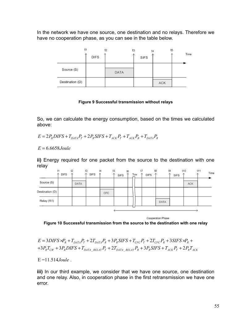
55

In the network we have one source, one destination and no relays. Therefore we have no cooperation phase, as you can see in the table below.

Figure 9 Successful transmission without relays

So, we can calculate the energy consumption, based on the times we calculated above:

ii) Energy required for one packet from the source to the destination with one relay

Figure 10 Successful transmission from the source to the destination with one relay

iii) In our third example, we consider that we have one source, one destination and one relay. Also, in cooperation phase in the first retransmission we have one error.

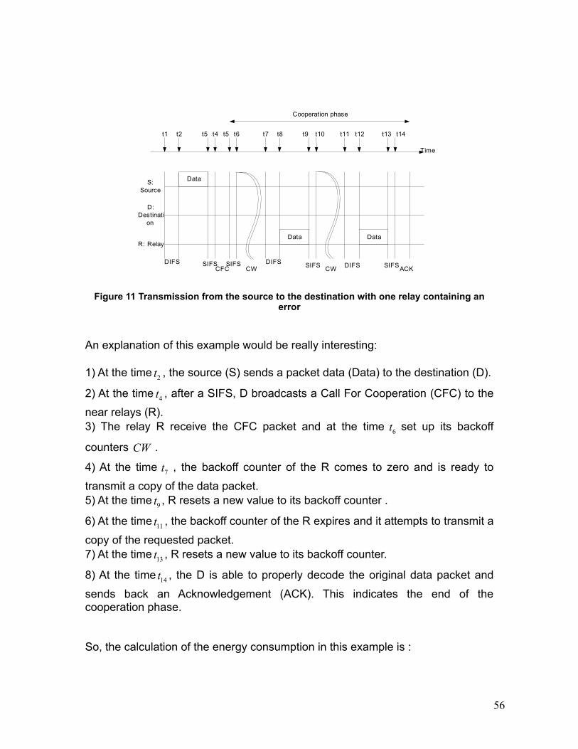
56

Figure 11 Transmission from the source to the destination with one relay containing an error

An explanation of this example would be really interesting:

1) At the time , the source (S) sends a packet data (Data) to the destination (D).

2) At the time , after a SIFS, D broadcasts a Call For Cooperation (CFC) to the

near relays (R).3) The relay R receive the CFC packet and at the time set up its backoff

counters .

4) At the time , the backoff counter of the R comes to zero and is ready to

transmit a copy of the data packet.5) At the time , R resets a new value to its backoff counter .

6) At the time , the backoff counter of the R expires and it attempts to transmit a

copy of the requested packet.7) At the time , R resets a new value to its backoff counter.

8) At the time , the D is able to properly decode the original data packet and

sends back an Acknowledgement (ACK). This indicates the end of the cooperation phase.

So, the calculation of the energy consumption in this example is :

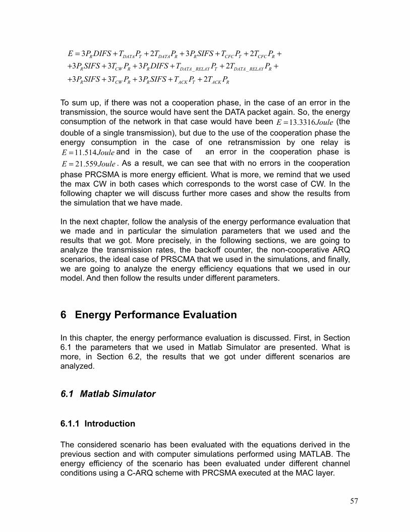
57

To sum up, if there was not a cooperation phase, in the case of an error in the transmission, the source would have sent the DATA packet again. So, the energy consumption of the network in that case would have been (the double of a single transmission), but due to the use of the cooperation phase the energy consumption in the case of one retransmission by one relay is

and in the case of an error in the cooperation phase is . As a result, we can see that with no errors in the cooperation

phase PRCSMA is more energy efficient. What is more, we remind that we used the max CW in both cases which corresponds to the worst case of CW. In the following chapter we will discuss further more cases and show the results from the simulation that we have made.

In the next chapter, follow the analysis of the energy performance evaluation that we made and in particular the simulation parameters that we used and the results that we got. More precisely, in the following sections, we are going to analyze the transmission rates, the backoff counter, the non-cooperative ARQ scenarios, the ideal case of PRSCMA that we used in the simulations, and finally, we are going to analyze the energy efficiency equations that we used in our model. And then follow the results under different parameters.

6 Energy Performance Evaluation

In this chapter, the energy performance evaluation is discussed. First, in Section 6.1 the parameters that we used in Matlab Simulator are presented. What is more, in Section 6.2, the results that we got under different scenarios are analyzed.

6.1 Matlab Simulator

6.1.1 Introduction

The considered scenario has been evaluated with the equations derived in the previous section and with computer simulations performed using MATLAB. The energy efficiency of the scenario has been evaluated under different channel conditions using a C-ARQ scheme with PRCSMA executed at the MAC layer.

58

More precisely, a comparison of the energy efficiency of the following three ARQ schemes is presented in this section:1) A non-cooperative ARQ scheme. In this scenario, retransmissions are requested directly from the source. Retransmissions are performed one after another, sequentially in time, and each retransmission is acknowledged, if received without errors, by the destination.2) A C-ARQ scheme where an ideal scheduling is attained among the relays. That is, the relays can ideally retransmit one after another without extra coordination overhead and with no collisions. In this case, each retransmission does not have to be acknowledged by the destination but a final ACK/NACK packet is transmitted at the end of the cooperation phase. This case is used as a reference theoretical upper bound.3) A C-ARQ scheme where the relays execute PRCSMA (both with the basic and the COLAV access modes).

In the following sections, we are going to define the transmission rates in 6.1.2, the backoff counter in 6.1.3, the non-cooperative ARQ scenarios in 6.1.4, the ideal case of PRSCMA that we used in the simulations in 6.1.5, and finally, we are going to analyze the energy efficiency equations that we used in our model in 6.1.6.

In the following session, we are going to explain the transmission rates we chose in the simulations.

6.1.2 Transmission Rates

In all cases, it is considered that transmissions from the source to any destination are performed at a constant transmission rate and another transmission rate for control information. These rates are referred to as the Source Control Rate (SCR) and Source Data Rate (SDR), respectively. On the other hand, retransmissions from the relays are performed also at two constant different rates, referred to as the Relay Control Rate (RCR) and Relay Data Rate (RDR).

Unless otherwise stated, it is considered that transmissions at the control plane are error-free and they are performed at 6Mbps, i.e., SCR=RCR=6 Mbps. Recall that this is the most robust modulation scheme of the IEEE 802.11g PHY (Physical) layers and that the length of control packets is much lower than that of data packets. Therefore, the packet error probability when transmitting a control packet is remarkably lower when transmitting a data packet.

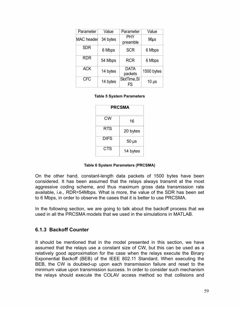
59

Table 5 System Parameters

Table 6 System Parameters (PRCSMA)

On the other hand, constant-length data packets of 1500 bytes have been considered. It has been assumed that the relays always transmit at the most aggressive coding scheme, and thus maximum gross data transmission rate available, i.e., RDR=54Mbps. What is more, the value of the SDR has been set to 6 Mbps, in order to observe the cases that it is better to use PRCSMA.

In the following section, we are going to talk about the backoff process that we used in all the PRCSMA models that we used in the simulations in MATLAB.

6.1.3 Backoff Counter

It should be mentioned that in the model presented in this section, we have assumed that the relays use a constant size of CW, but this can be used as a relatively good approximation for the case when the relays execute the Binary Exponential Backoff (BEB) of the IEEE 802.11 Standard. When executing the BEB, the CW is doubled-up upon each transmission failure and reset to the minimum value upon transmission success. In order to consider such mechanism the relays should execute the COLAV access method so that collisions and

60

transmissions errors can be detected in the cooperation phase. Recall that in the regular operator of a PRCSMA cooperation phase there is no ACK expected for each retransmission and thus, with the basic access method, a relay cannot be aware of whether the retransmission was successfully received by the destination or not and no adjustments of the backoff window can be performed.

The results in this section are focused on the overall network energy efficiency. In addition, a comparison with the energy efficiency obtained when using the non-cooperative ARQ scheme is also included. And this is the topic of the next session.

6.1.4 Non-cooperative ARQIn this section it is defined the case of non-cooperative ARQ sceme. For this case, are taken into account two scenarios.

Scenario 1

In the first scenario, we measured the energy only of the source and the destination. So, this scenario is not taking into account the energy consumption of all the nodes that consist the network. We assumed that when the source sends an erroneous packet to the destination it is obligated to send it again and again, until the destination can decode correctly the packet. Recall that the control transmission rate from source to the destination is 6 Mbps, and the data transmission rate from source to the destination is also 6 Mbps. Under these parameters, we expect that this scenario will be comparable only when we use PRCSMA with a small number of potential relays, which fact we analyze in the following chapters.

Scenario 2

On the other hand, in the second scenario of the non-cooperative case, it is assumed again that when the source sends an erroneous packet to the destination, it has to send it again, until the destination gets the correct packet. But, in this case we are taking into account the energy consumption of the whole network, which means that except from the source and the destination we measure the energy consumption of the potential relays as nodes who just receive the packets sent by the source and do nothing but overhear. This scenario is more comparable with PRCSMA scenarios, because as we have already said, takes into account the energy consumption of the whole network and not only of the source and the destination and as we are going to show in the following chapters, in most of the cases PRCSMA outperforms non-cooperative ARQ (scenario 2) in terms of energy efficiency.

In the next session, we are going to present the ideal scenarios of PRCSMA that we included in our simulations, to show what will happen if there is perfect

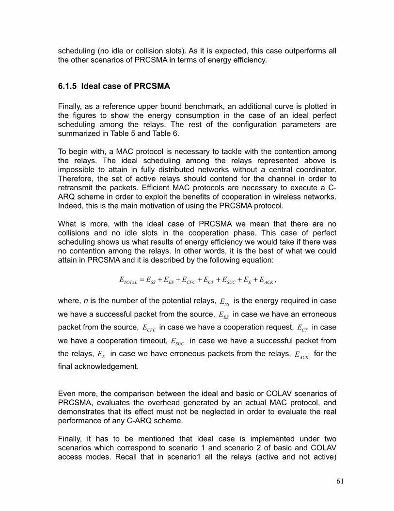
61

scheduling (no idle or collision slots). As it is expected, this case outperforms all the other scenarios of PRCSMA in terms of energy efficiency.

6.1.5 Ideal case of PRCSMA

Finally, as a reference upper bound benchmark, an additional curve is plotted in the figures to show the energy consumption in the case of an ideal perfect scheduling among the relays. The rest of the configuration parameters are summarized in Table 5 and Table 6.

To begin with, a MAC protocol is necessary to tackle with the contention among the relays. The ideal scheduling among the relays represented above is impossible to attain in fully distributed networks without a central coordinator. Therefore, the set of active relays should contend for the channel in order to retransmit the packets. Efficient MAC protocols are necessary to execute a C-ARQ scheme in order to exploit the benefits of cooperation in wireless networks. Indeed, this is the main motivation of using the PRCSMA protocol.

What is more, with the ideal case of PRCSMA we mean that there are no collisions and no idle slots in the cooperation phase. This case of perfect scheduling shows us what results of energy efficiency we would take if there was no contention among the relays. In other words, it is the best of what we could attain in PRCSMA and it is described by the following equation:

where, n is the number of the potential relays, is the energy required in case

we have a successful packet from the source, in case we have an erroneous

packet from the source, in case we have a cooperation request, in case

we have a cooperation timeout, in case we have a successful packet from

the relays, in case we have erroneous packets from the relays, for the

final acknowledgement.

Even more, the comparison between the ideal and basic or COLAV scenarios of PRCSMA, evaluates the overhead generated by an actual MAC protocol, and demonstrates that its effect must not be neglected in order to evaluate the real performance of any C-ARQ scheme.

Finally, it has to be mentioned that ideal case is implemented under two scenarios which correspond to scenario 1 and scenario 2 of basic and COLAV access modes. Recall that in scenario1 all the relays (active and not active)

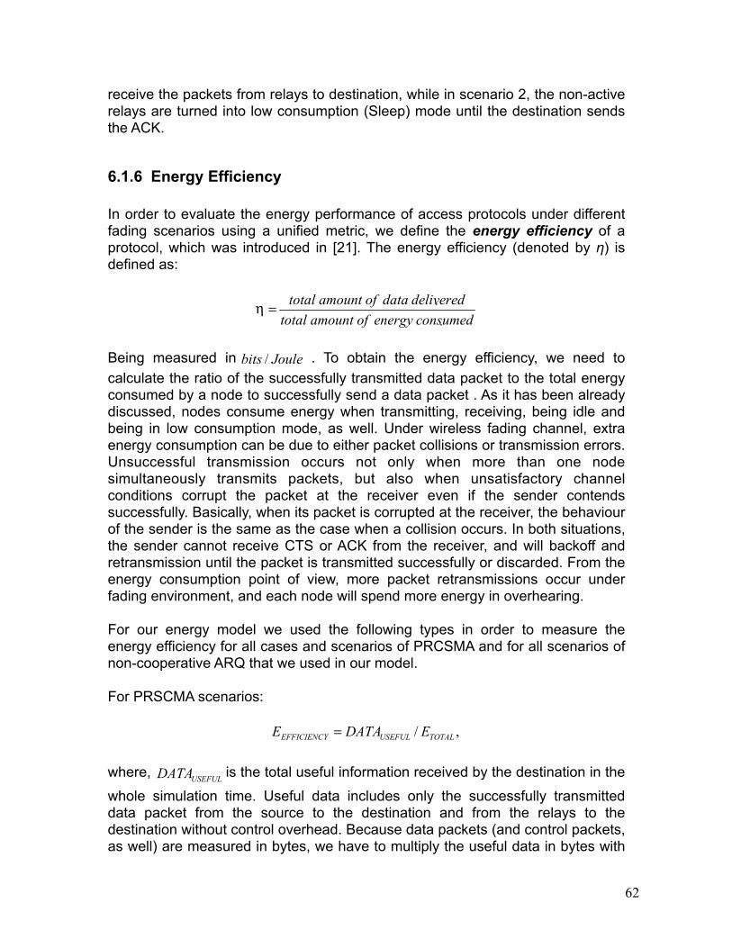
62

receive the packets from relays to destination, while in scenario 2, the non-active relays are turned into low consumption (Sleep) mode until the destination sends the ACK.

6.1.6 Energy Efficiency

In order to evaluate the energy performance of access protocols under different fading scenarios using a unified metric, we define the energy efficiency of a protocol, which was introduced in [21]. The energy efficiency (denoted by η) is defined as:

Being measured in . To obtain the energy efficiency, we need to calculate the ratio of the successfully transmitted data packet to the total energy consumed by a node to successfully send a data packet . As it has been already discussed, nodes consume energy when transmitting, receiving, being idle and being in low consumption mode, as well. Under wireless fading channel, extra energy consumption can be due to either packet collisions or transmission errors. Unsuccessful transmission occurs not only when more than one node simultaneously transmits packets, but also when unsatisfactory channel conditions corrupt the packet at the receiver even if the sender contends successfully. Basically, when its packet is corrupted at the receiver, the behaviour of the sender is the same as the case when a collision occurs. In both situations, the sender cannot receive CTS or ACK from the receiver, and will backoff and retransmission until the packet is transmitted successfully or discarded. From the energy consumption point of view, more packet retransmissions occur under fading environment, and each node will spend more energy in overhearing.

For our energy model we used the following types in order to measure the energy efficiency for all cases and scenarios of PRCSMA and for all scenarios of non-cooperative ARQ that we used in our model.

For PRSCMA scenarios:

where, is the total useful information received by the destination in the

whole simulation time. Useful data includes only the successfully transmitted data packet from the source to the destination and from the relays to the destination without control overhead. Because data packets (and control packets, as well) are measured in bytes, we have to multiply the useful data in bytes with

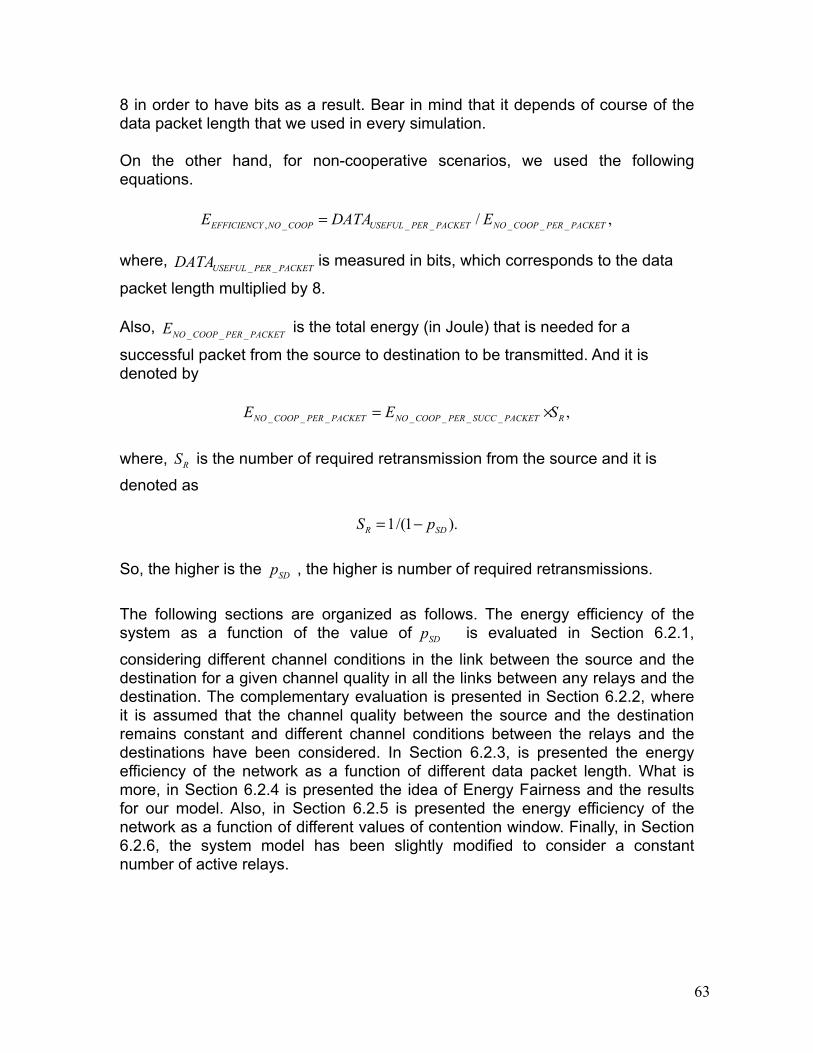
63

8 in order to have bits as a result. Bear in mind that it depends of course of the data packet length that we used in every simulation.

On the other hand, for non-cooperative scenarios, we used the following equations.

where, is measured in bits, which corresponds to the data

packet length multiplied by 8.

Also, is the total energy (in Joule) that is needed for a

successful packet from the source to destination to be transmitted. And it is denoted by

where, is the number of required retransmission from the source and it is

denoted as

So, the higher is the , the higher is number of required retransmissions.

The following sections are organized as follows. The energy efficiency of the system as a function of the value of is evaluated in Section 6.2.1,

considering different channel conditions in the link between the source and the destination for a given channel quality in all the links between any relays and the destination. The complementary evaluation is presented in Section 6.2.2, where it is assumed that the channel quality between the source and the destination remains constant and different channel conditions between the relays and the destinations have been considered. In Section 6.2.3, is presented the energy efficiency of the network as a function of different data packet length. What is more, in Section 6.2.4 is presented the idea of Energy Fairness and the results for our model. Also, in Section 6.2.5 is presented the energy efficiency of the network as a function of different values of contention window. Finally, in Section 6.2.6, the system model has been slightly modified to consider a constant number of active relays.

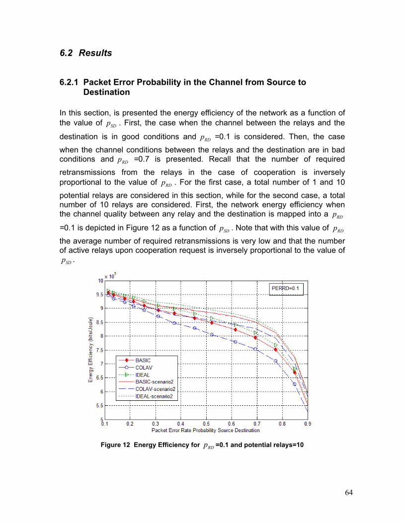
64

6.2 Results

6.2.1 Packet Error Probability in the Channel from Source to Destination

In this section, is presented the energy efficiency of the network as a function of the value of . First, the case when the channel between the relays and the

destination is in good conditions and =0.1 is considered. Then, the case

when the channel conditions between the relays and the destination are in bad conditions and =0.7 is presented. Recall that the number of required

retransmissions from the relays in the case of cooperation is inversely proportional to the value of . For the first case, a total number of 1 and 10

potential relays are considered in this section, while for the second case, a total number of 10 relays are considered. First, the network energy efficiency when the channel quality between any relay and the destination is mapped into a

=0.1 is depicted in Figure 12 as a function of . Note that with this value of

the average number of required retransmissions is very low and that the number of active relays upon cooperation request is inversely proportional to the value of

.

Figure 12 Energy Efficiency for =0.1 and potential relays=10

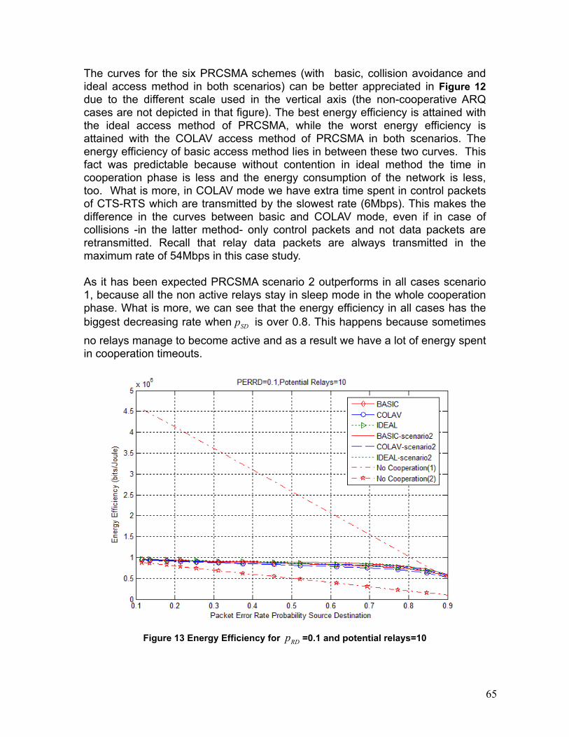
65

The curves for the six PRCSMA schemes (with basic, collision avoidance and ideal access method in both scenarios) can be better appreciated in Figure 12 due to the different scale used in the vertical axis (the non-cooperative ARQ cases are not depicted in that figure). The best energy efficiency is attained with the ideal access method of PRCSMA, while the worst energy efficiency is attained with the COLAV access method of PRCSMA in both scenarios. The energy efficiency of basic access method lies in between these two curves. This fact was predictable because without contention in ideal method the time in cooperation phase is less and the energy consumption of the network is less, too. What is more, in COLAV mode we have extra time spent in control packets of CTS-RTS which are transmitted by the slowest rate (6Mbps). This makes the difference in the curves between basic and COLAV mode, even if in case of collisions -in the latter method- only control packets and not data packets are retransmitted. Recall that relay data packets are always transmitted in the maximum rate of 54Mbps in this case study.

As it has been expected PRCSMA scenario 2 outperforms in all cases scenario 1, because all the non active relays stay in sleep mode in the whole cooperation phase. What is more, we can see that the energy efficiency in all cases has the biggest decreasing rate when is over 0.8. This happens because sometimes

no relays manage to become active and as a result we have a lot of energy spent in cooperation timeouts.

Figure 13 Energy Efficiency for =0.1 and potential relays=10

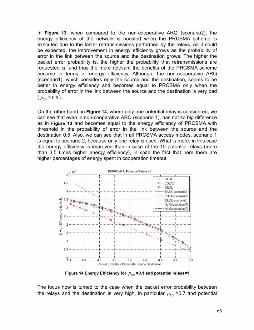
66

In Figure 13, when compared to the non-cooperative ARQ (scenario2), the energy efficiency of the network is boosted when the PRCSMA scheme is executed due to the faster retransmissions performed by the relays. As it could be expected, the improvement in energy efficiency grows as the probability of error in the link between the source and the destination grows. The higher the packet error probability is, the higher the probability that retransmissions are requested is, and thus the more relevant the benefits of the PRCSMA scheme become in terms of energy efficiency. Although, the non-cooperative ARQ (scenario1), which considers only the source and the destination, seems to be better in energy efficiency and becomes equal to PRCSMA only when the probability of error in the link between the source and the destination is very bad ( ) .

On the other hand, in Figure 14, where only one potential relay is considered, we can see that even in non-cooperative ARQ (scenario 1), has not so big difference as in Figure 13 and becomes equal to the energy efficiency of PRCSMA with threshold in the probability of error in the link between the source and the destination 0.5. Also, we can see that in all PRCSMA access modes, scenario 1 is equal to scenario 2, because only one relay is used. What is more, in this case the energy efficiency is improved than in case of the 10 potential relays (more than 3.5 times higher energy efficiency), in spite the fact that here there are higher percentages of energy spent in cooperation timeout.

Figure 14 Energy Efficiency for =0.1 and potential relays=1

The focus now is turned to the case when the packet error probability between the relays and the destination is very high, in particular =0.7 and potential

67

relays are 10. The energy efficiency of the network is depicted in Figure 15 as a function of the six PRCSMA schemes (with basic, collision avoidance and ideal access method in both scenarios). The curves can be better appreciated in Figure 15 due to the different scale used in the vertical axis, (the non-cooperative ARQ (scenario1) is not depicted in that figure because as we can assume from Figure 13, it outperforms with a big difference PRCSMA).

Under these conditions, the number of required retransmissions from the relays is greater than in the previous case due to the higher probability of packet error in a retransmission, and thus the effects of the contention process among the relays become more remarkable. So, the time in cooperation phase grows, and the difference in energy consumption between the active and the non-active relays in PRCSMA scenarios 2 becomes more obvious as we can see in the curves. As a result, the energy saving under PRCSMA scenario 2 in this case is important.

Despite the higher probability of packet error in a retransmission from the relays, all the PRCSMA schemes considered in this scenario outperform non-cooperative ARQ (scenario2) in all cases. The reason for that is that despite the higher probability of error in the link between the relays and the destination, the cost of a failed retransmission is much lower from the relays than from the source in terms of channel occupancy time. Therefore, it is better in this case to call for cooperation to that relays which have an error-free copy of the original packet rather than requesting retransmission from the source, which will transmit at a considerably lower transmission rate.

What is more, the case with =0.7 and potential relays=1, is not depicted here

because it is almost the same figure as Figure 14. The only difference is that non-cooperative ARQ (scenario 2) outperforms PRCSMA in terms of energy efficiency with threshold of =0.6, when in Figure 14, the threshold was =0.5. This

can be explained easily because of the worse quality in cannel from relay to destination.

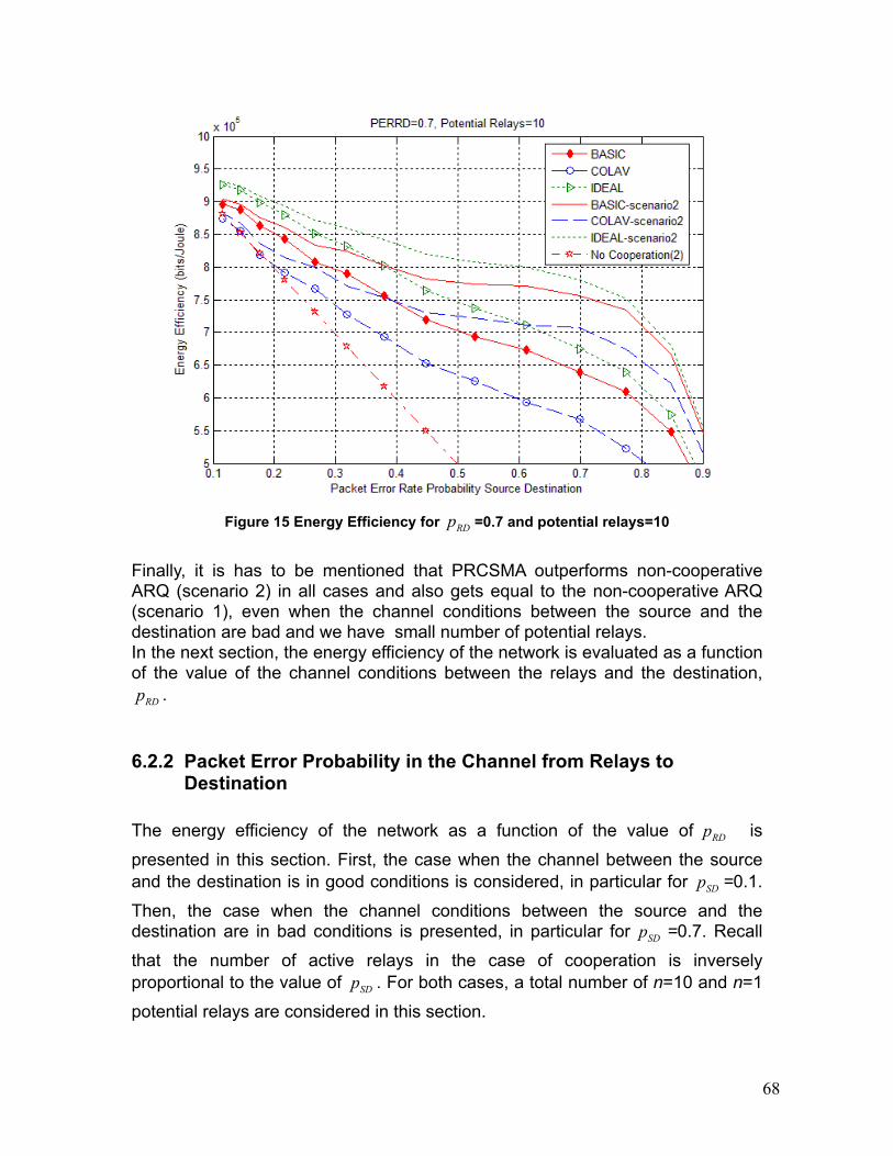
68

Figure 15 Energy Efficiency for =0.7 and potential relays=10

Finally, it is has to be mentioned that PRCSMA outperforms non-cooperative ARQ (scenario 2) in all cases and also gets equal to the non-cooperative ARQ (scenario 1), even when the channel conditions between the source and the destination are bad and we have small number of potential relays.In the next section, the energy efficiency of the network is evaluated as a function of the value of the channel conditions between the relays and the destination,

.

6.2.2 Packet Error Probability in the Channel from Relays to Destination

The energy efficiency of the network as a function of the value of is

presented in this section. First, the case when the channel between the source and the destination is in good conditions is considered, in particular for =0.1.

Then, the case when the channel conditions between the source and the destination are in bad conditions is presented, in particular for =0.7. Recall

that the number of active relays in the case of cooperation is inversely proportional to the value of . For both cases, a total number of n=10 and n=1

potential relays are considered in this section.

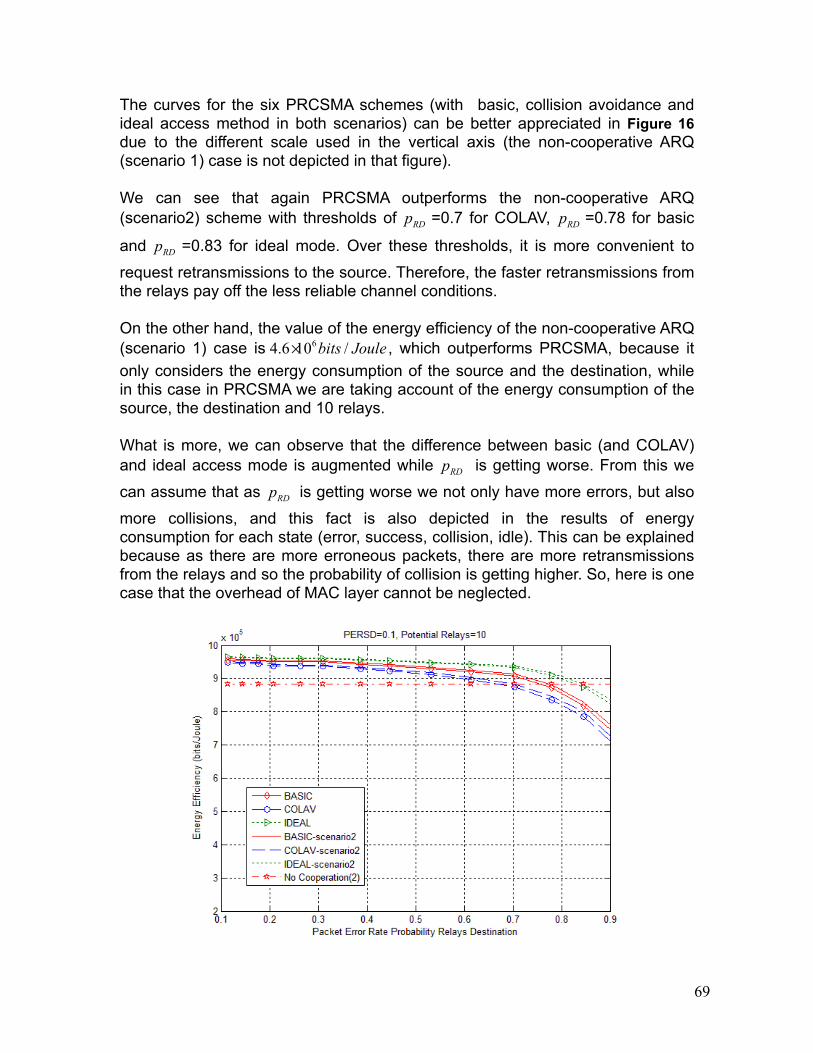
69

The curves for the six PRCSMA schemes (with basic, collision avoidance and ideal access method in both scenarios) can be better appreciated in Figure 16 due to the different scale used in the vertical axis (the non-cooperative ARQ (scenario 1) case is not depicted in that figure).

We can see that again PRCSMA outperforms the non-cooperative ARQ (scenario2) scheme with thresholds of =0.7 for COLAV, =0.78 for basic

and =0.83 for ideal mode. Over these thresholds, it is more convenient to

request retransmissions to the source. Therefore, the faster retransmissions from the relays pay off the less reliable channel conditions.

On the other hand, the value of the energy efficiency of the non-cooperative ARQ (scenario 1) case is , which outperforms PRCSMA, because it only considers the energy consumption of the source and the destination, while in this case in PRCSMA we are taking account of the energy consumption of the source, the destination and 10 relays.

What is more, we can observe that the difference between basic (and COLAV) and ideal access mode is augmented while is getting worse. From this we

can assume that as is getting worse we not only have more errors, but also

more collisions, and this fact is also depicted in the results of energy consumption for each state (error, success, collision, idle). This can be explained because as there are more erroneous packets, there are more retransmissions from the relays and so the probability of collision is getting higher. So, here is one case that the overhead of MAC layer cannot be neglected.

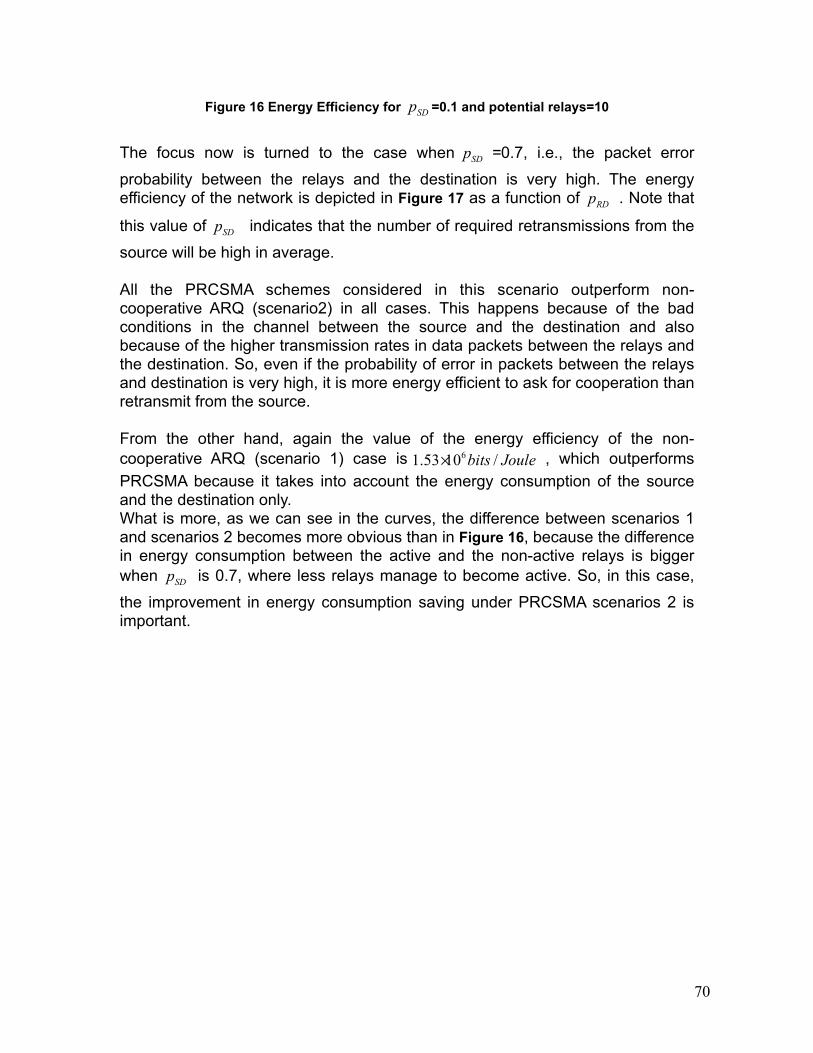
70

Figure 16 Energy Efficiency for =0.1 and potential relays=10

The focus now is turned to the case when =0.7, i.e., the packet error

probability between the relays and the destination is very high. The energy efficiency of the network is depicted in Figure 17 as a function of . Note that

this value of indicates that the number of required retransmissions from the

source will be high in average.

All the PRCSMA schemes considered in this scenario outperform non-cooperative ARQ (scenario2) in all cases. This happens because of the bad conditions in the channel between the source and the destination and also because of the higher transmission rates in data packets between the relays and the destination. So, even if the probability of error in packets between the relays and destination is very high, it is more energy efficient to ask for cooperation than retransmit from the source.

From the other hand, again the value of the energy efficiency of the non-cooperative ARQ (scenario 1) case is , which outperforms PRCSMA because it takes into account the energy consumption of the source and the destination only.What is more, as we can see in the curves, the difference between scenarios 1 and scenarios 2 becomes more obvious than in Figure 16, because the difference in energy consumption between the active and the non-active relays is bigger when is 0.7, where less relays manage to become active. So, in this case,

the improvement in energy consumption saving under PRCSMA scenarios 2 is important.

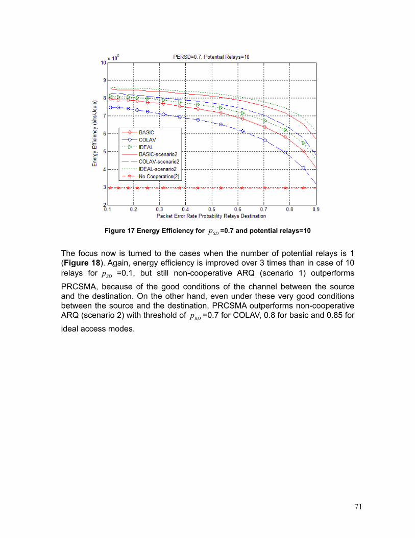
71

Figure 17 Energy Efficiency for =0.7 and potential relays=10

The focus now is turned to the cases when the number of potential relays is 1 (Figure 18). Again, energy efficiency is improved over 3 times than in case of 10 relays for =0.1, but still non-cooperative ARQ (scenario 1) outperforms

PRCSMA, because of the good conditions of the channel between the source and the destination. On the other hand, even under these very good conditions between the source and the destination, PRCSMA outperforms non-cooperative ARQ (scenario 2) with threshold of =0.7 for COLAV, 0.8 for basic and 0.85 for

ideal access modes.

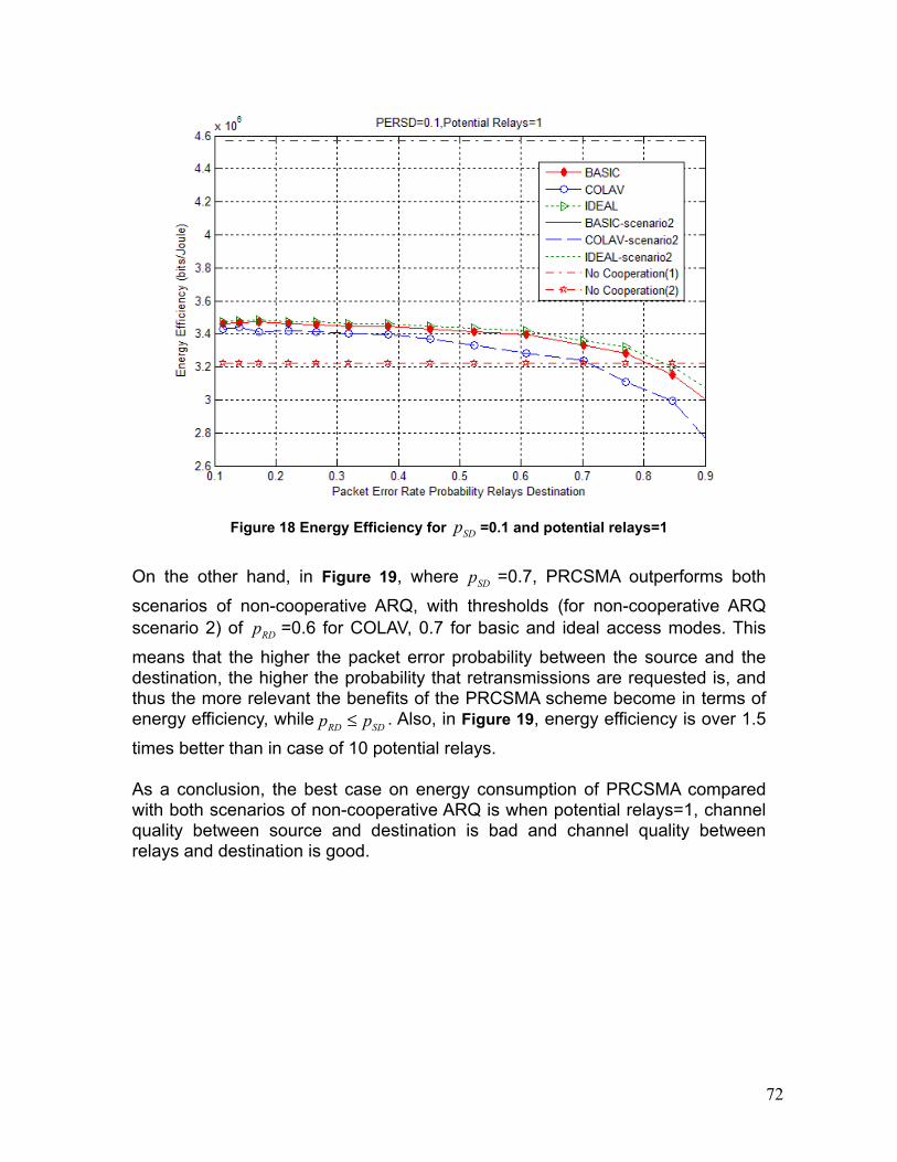
72

Figure 18 Energy Efficiency for =0.1 and potential relays=1

On the other hand, in Figure 19, where =0.7, PRCSMA outperforms both

scenarios of non-cooperative ARQ, with thresholds (for non-cooperative ARQ scenario 2) of =0.6 for COLAV, 0.7 for basic and ideal access modes. This

means that the higher the packet error probability between the source and the destination, the higher the probability that retransmissions are requested is, and thus the more relevant the benefits of the PRCSMA scheme become in terms of energy efficiency, while . Also, in Figure 19, energy efficiency is over 1.5

times better than in case of 10 potential relays.

As a conclusion, the best case on energy consumption of PRCSMA compared with both scenarios of non-cooperative ARQ is when potential relays=1, channel quality between source and destination is bad and channel quality between relays and destination is good.

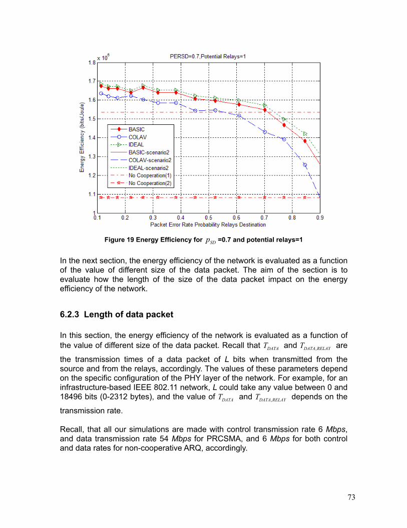
73

Figure 19 Energy Efficiency for =0.7 and potential relays=1

In the next section, the energy efficiency of the network is evaluated as a function of the value of different size of the data packet. The aim of the section is to evaluate how the length of the size of the data packet impact on the energy efficiency of the network.

6.2.3 Length of data packet

In this section, the energy efficiency of the network is evaluated as a function of the value of different size of the data packet. Recall that and are

the transmission times of a data packet of L bits when transmitted from the source and from the relays, accordingly. The values of these parameters depend on the specific configuration of the PHY layer of the network. For example, for an infrastructure-based IEEE 802.11 network, L could take any value between 0 and 18496 bits (0-2312 bytes), and the value of and depends on the

transmission rate.

Recall, that all our simulations are made with control transmission rate 6 Mbps, and data transmission rate 54 Mbps for PRCSMA, and 6 Mbps for both control and data rates for non-cooperative ARQ, accordingly.

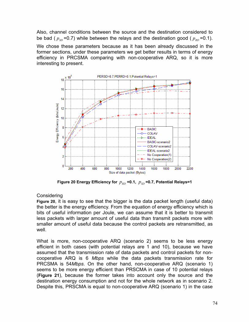
74

Also, channel conditions between the source and the destination considered to be bad ( =0.7) while between the relays and the destination good ( =0.1).

We chose these parameters because as it has been already discussed in the former sections, under these parameters we get better results in terms of energy efficiency in PRCSMA comparing with non-cooperative ARQ, so it is more interesting to present.

Figure 20 Energy Efficiency for =0.1, =0.7, Potential Relays=1

Considering Figure 20, it is easy to see that the bigger is the data packet length (useful data) the better is the energy efficiency. From the equation of energy efficiency which is bits of useful information per Joule, we can assume that it is better to transmit less packets with larger amount of useful data than transmit packets more with smaller amount of useful data because the control packets are retransmitted, as well.

What is more, non-cooperative ARQ (scenario 2) seems to be less energy efficient in both cases (with potential relays are 1 and 10), because we have assumed that the transmission rate of data packets and control packets for non-cooperative ARQ is 6 Mbps while the data packets transmission rate for PRCSMA is 54Mbps. On the other hand, non-cooperative ARQ (scenario 1) seems to be more energy efficient than PRSCMA in case of 10 potential relays (Figure 21), because the former takes into account only the source and the destination energy consumption and not for the whole network as in scenario 2. Despite this, PRSCMA is equal to non-cooperative ARQ (scenario 1) in the case

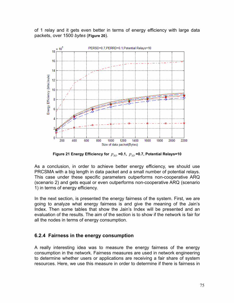
75

of 1 relay and it gets even better in terms of energy efficiency with large data packets, over 1500 bytes (Figure 20).

Figure 21 Energy Efficiency for =0.1, =0.7, Potential Relays=10

As a conclusion, in order to achieve better energy efficiency, we should use PRCSMA with a big length in data packet and a small number of potential relays. This case under these specific parameters outperforms non-cooperative ARQ (scenario 2) and gets equal or even outperforms non-cooperative ARQ (scenario 1) in terms of energy efficiency. In the next section, is presented the energy fairness of the system. First, we are going to analyze what energy fairness is and give the meaning of the Jain’s Index. Then some tables that show the Jain’s Index will be presented and an evaluation of the results. The aim of the section is to show if the network is fair for all the nodes in terms of energy consumption.

6.2.4 Fairness in the energy consumption

A really interesting idea was to measure the energy fairness of the energy consumption in the network. Fairness measures are used in network engineering to determine whether users or applications are receiving a fair share of system resources. Here, we use this measure in order to determine if there is fairness in

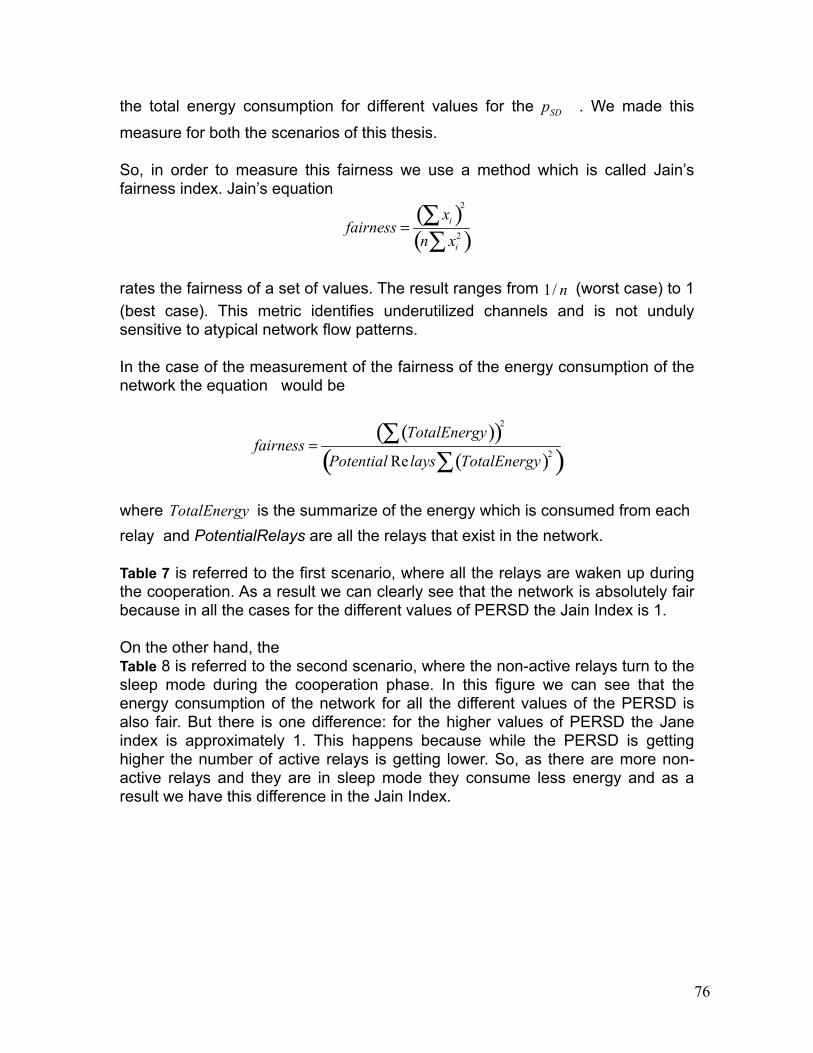
76

the total energy consumption for different values for the . We made this

measure for both the scenarios of this thesis.

So, in order to measure this fairness we use a method which is called Jain’s fairness index. Jain’s equation

rates the fairness of a set of values. The result ranges from (worst case) to 1 (best case). This metric identifies underutilized channels and is not unduly sensitive to atypical network flow patterns.

In the case of the measurement of the fairness of the energy consumption of the network the equation would be

where is the summarize of the energy which is consumed from each relay and PotentialRelays are all the relays that exist in the network.

Table 7 is referred to the first scenario, where all the relays are waken up during the cooperation. As a result we can clearly see that the network is absolutely fair because in all the cases for the different values of PERSD the Jain Index is 1.

On the other hand, the Table 8 is referred to the second scenario, where the non-active relays turn to the sleep mode during the cooperation phase. In this figure we can see that the energy consumption of the network for all the different values of the PERSD is also fair. But there is one difference: for the higher values of PERSD the Jane index is approximately 1. This happens because while the PERSD is getting higher the number of active relays is getting lower. So, as there are more non-active relays and they are in sleep mode they consume less energy and as a result we have this difference in the Jain Index.

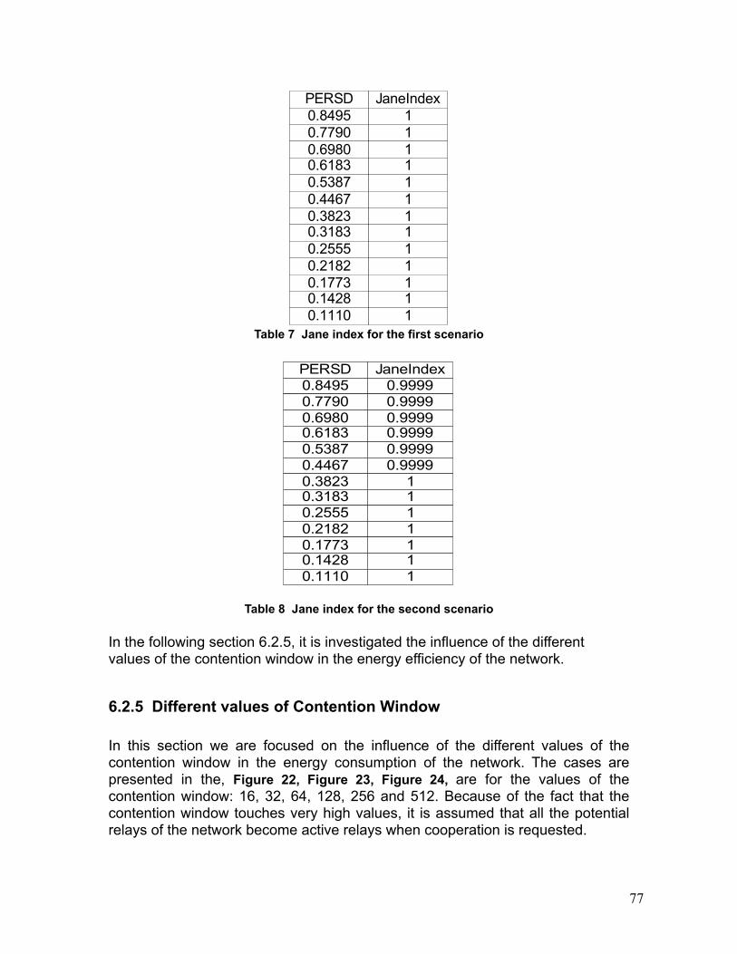
77

Table 7 Jane index for the first scenario

Table 8 Jane index for the second scenario

In the following section 6.2.5, it is investigated the influence of the different values of the contention window in the energy efficiency of the network.

6.2.5 Different values of Contention Window

In this section we are focused on the influence of the different values of the contention window in the energy consumption of the network. The cases are presented in the, Figure 22, Figure 23, Figure 24, are for the values of the contention window: 16, 32, 64, 128, 256 and 512. Because of the fact that the contention window touches very high values, it is assumed that all the potential relays of the network become active relays when cooperation is requested.

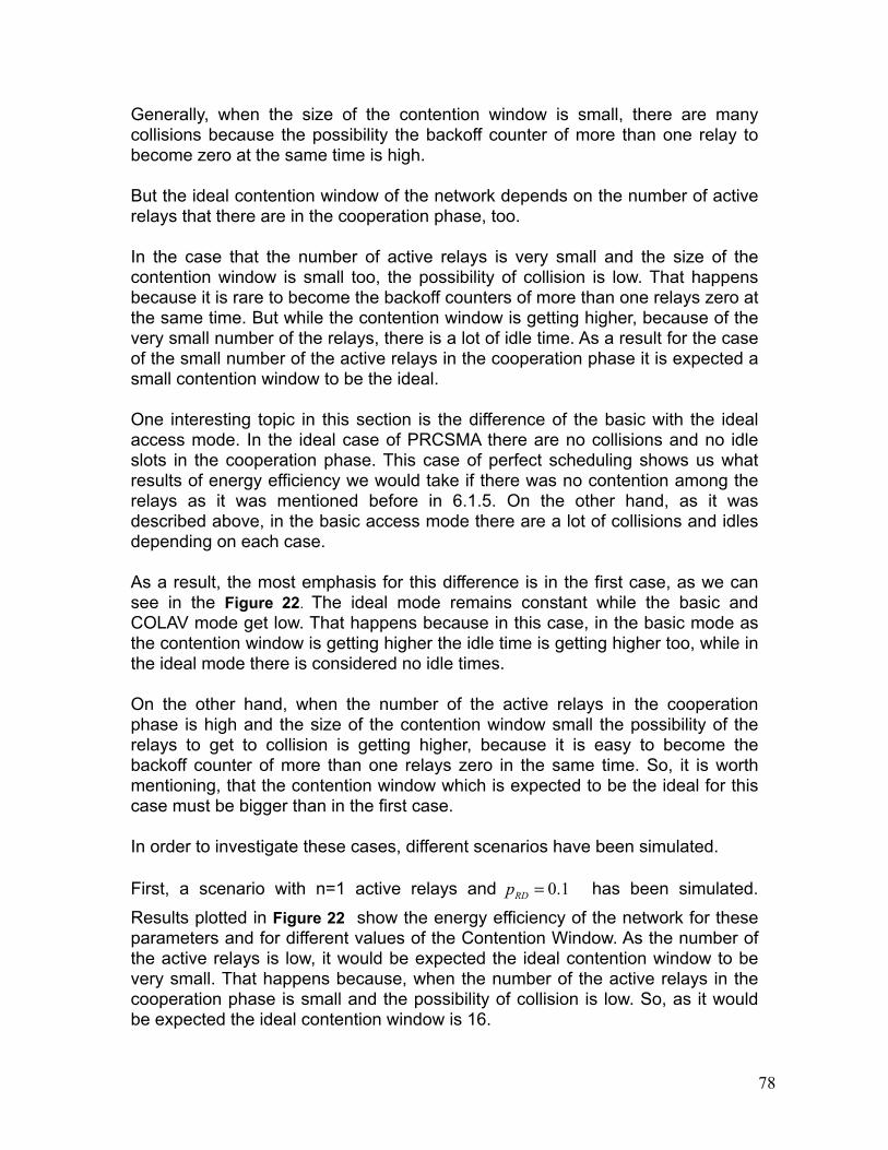
78

Generally, when the size of the contention window is small, there are many collisions because the possibility the backoff counter of more than one relay to become zero at the same time is high.

But the ideal contention window of the network depends on the number of active relays that there are in the cooperation phase, too.

In the case that the number of active relays is very small and the size of the contention window is small too, the possibility of collision is low. That happens because it is rare to become the backoff counters of more than one relays zero at the same time. But while the contention window is getting higher, because of the very small number of the relays, there is a lot of idle time. As a result for the case of the small number of the active relays in the cooperation phase it is expected a small contention window to be the ideal.

One interesting topic in this section is the difference of the basic with the ideal access mode. In the ideal case of PRCSMA there are no collisions and no idle slots in the cooperation phase. This case of perfect scheduling shows us what results of energy efficiency we would take if there was no contention among the relays as it was mentioned before in 6.1.5. On the other hand, as it was described above, in the basic access mode there are a lot of collisions and idles depending on each case.

As a result, the most emphasis for this difference is in the first case, as we can see in the Figure 22. The ideal mode remains constant while the basic and COLAV mode get low. That happens because in this case, in the basic mode as the contention window is getting higher the idle time is getting higher too, while in the ideal mode there is considered no idle times.

On the other hand, when the number of the active relays in the cooperation phase is high and the size of the contention window small the possibility of the relays to get to collision is getting higher, because it is easy to become the backoff counter of more than one relays zero in the same time. So, it is worth mentioning, that the contention window which is expected to be the ideal for this case must be bigger than in the first case.

In order to investigate these cases, different scenarios have been simulated.

First, a scenario with n=1 active relays and has been simulated.

Results plotted in Figure 22 show the energy efficiency of the network for these parameters and for different values of the Contention Window. As the number of the active relays is low, it would be expected the ideal contention window to be very small. That happens because, when the number of the active relays in the cooperation phase is small and the possibility of collision is low. So, as it would be expected the ideal contention window is 16.

79

The scenario which has been simulated afterwards, was that with n=5 active relays and . It is worth mentioning that the ideal contention window is

expected to be bigger than the previous one (contention window: 16) but still small as the number of the potential relays remains low. So, as it is shown in the Figure 23 the ideal contention window for this case is 32.

On the other hand, it has also simulated another scenario with n=15 active relays, as it is shown in Figure 23. As the number of the active relays in the cooperation phase getting higher the possibility of collision is getting higher too. The higher the number of active relays, the higher the ideal contention window. As it shown in Figure 24, the ideal contention window is 64.

Figure 22 Energy Efficiency for 1 active relay as a function of the contention window

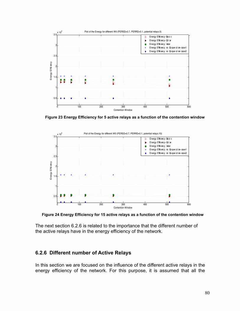
80

Figure 23 Energy Efficiency for 5 active relays as a function of the contention window

Figure 24 Energy Efficiency for 15 active relays as a function of the contention window

The next section 6.2.6 is related to the importance that the different number of the active relays have in the energy efficiency of the network.

6.2.6 Different number of Active Relays

In this section we are focused on the influence of the different active relays in the energy efficiency of the network. For this purpose, it is assumed that all the

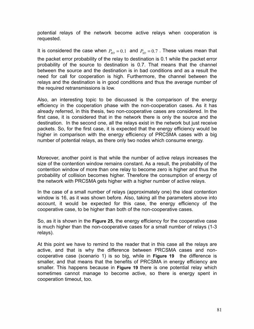
81

potential relays of the network become active relays when cooperation is requested.

It is considered the case when and . These values mean that

the packet error probability of the relay to destination is 0.1 while the packet error probability of the source to destination is 0.7. That means that the channel between the source and the destination is in bad conditions and as a result the need for call for cooperation is high. Furthermore, the channel between the relays and the destination is in good conditions and thus the average number of the required retransmissions is low.

Also, an interesting topic to be discussed is the comparison of the energy efficiency in the cooperation phase with the non-cooperation cases. As it has already referred, in this thesis, two non-cooperative cases are considered. In the first case, it is considered that in the network there is only the source and the destination. In the second one, all the relays exist in the network but just receive packets. So, for the first case, it is expected that the energy efficiency would be higher in comparison with the energy efficiency of PRCSMA cases with a big number of potential relays, as there only two nodes which consume energy.

Moreover, another point is that while the number of active relays increases the size of the contention window remains constant. As a result, the probability of the contention window of more than one relay to become zero is higher and thus the probability of collision becomes higher. Therefore the consumption of energy of the network with PRCSMA gets higher with a higher number of active relays.

In the case of a small number of relays (approximately one) the ideal contention window is 16, as it was shown before. Also, taking all the parameters above into account, it would be expected for this case, the energy efficiency of the cooperative case, to be higher than both of the non-cooperative cases.

So, as it is shown in the Figure 25, the energy efficiency for the cooperative case is much higher than the non-cooperative cases for a small number of relays (1-3 relays).

At this point we have to remind to the reader that in this case all the relays are active, and that is why the difference between PRCSMA cases and non-cooperative case (scenario 1) is so big, while in Figure 19 the difference is smaller, and that means that the benefits of PRCSMA in energy efficiency are smaller. This happens because in Figure 19 there is one potential relay which sometimes cannot manage to become active, so there is energy spent in cooperation timeout, too.

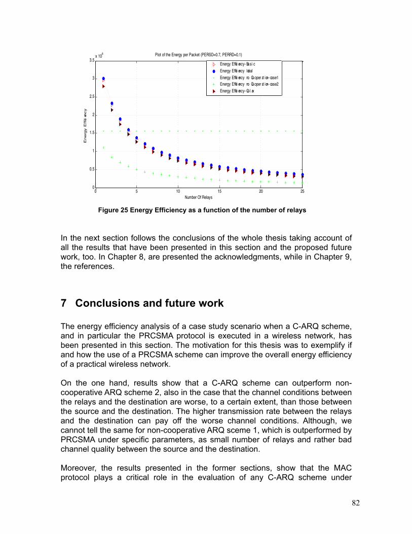
82

Figure 25 Energy Efficiency as a function of the number of relays

In the next section follows the conclusions of the whole thesis taking account of all the results that have been presented in this section and the proposed future work, too. In Chapter 8, are presented the acknowledgments, while in Chapter 9, the references.

7 Conclusions and future work

The energy efficiency analysis of a case study scenario when a C-ARQ scheme, and in particular the PRCSMA protocol is executed in a wireless network, has been presented in this section. The motivation for this thesis was to exemplify if and how the use of a PRCSMA scheme can improve the overall energy efficiency of a practical wireless network.

On the one hand, results show that a C-ARQ scheme can outperform non-cooperative ARQ scheme 2, also in the case that the channel conditions between the relays and the destination are worse, to a certain extent, than those between the source and the destination. The higher transmission rate between the relays and the destination can pay off the worse channel conditions. Although, we cannot tell the same for non-cooperative ARQ sceme 1, which is outperformed by PRCSMA under specific parameters, as small number of relays and rather bad channel quality between the source and the destination.

Moreover, the results presented in the former sections, show that the MAC protocol plays a critical role in the evaluation of any C-ARQ scheme under

83

specific network conditions. It has been shown that the time required for contention cannot be neglected, especially under some network conditions. When either there are a high number of relays contending for the channel to retransmit or more than one retransmission is needed from the relays (high traffic load), or when the number of relays is small and the Contention Window is high. In these cases, the idealization of the contention time due to the MAC problem can lead to wrong conclusions regarding the energy efficiency of C-ARQ.

Therefore, an efficient MAC protocol is necessary to efficiently coordinate the relay retransmissions in a C-ARQ scheme so that a performance close to the ideal perfect scheduling can be attained. The results presented in PRCSMA, is that attains the best energy efficiency in very simple scenarios with low number of required retransmissions and with a low number of active relays in addition with small CW.

The main contributions of this part of the thesis have been:1) Design, analysis, and energy efficiency evaluation of PRCSMA, as an innovative MAC protocol for C-ARQ schemes based on the IEEE 802.11 Standard.2) Comparison of five different ARQ schemes, considering two non-cooperative schemes, ideal C-ARQ, C-ARQ with PRCSMA basic access mode, and C-ARQ with PRCSMA COLAV access mode. Plus, consideration of all the PRCSMA schemes under two scenarios, where scenario 1 is without sleep mode, while scenario 2 is with consideration of sleep mode. This also leads to improvement of the energy consumption of the PRCSMA protocol.3) Comparison of PRCSMA with basic or COLAV access mode and ideal case. Identification of the cases where MAC overhead cannot be neglected.4) Evaluation of the energy fairness of the relays that consist the network, in order to see if all the relays consume the same amount of energy under this protocol.

More analytically, the energy efficiency of five different ARQ schemes have been compared: two non-cooperative ARQ schemes wherein retransmissions are requested from the source, and three C-ARQ schemes with ideal scheduling, PRCSMA with basic access mode, and PRCSMA with COLAV access mode have been considered.

What is more, a case study consisting of a source, a destination and a number of distant stations has been analyzed. Whenever a packet is received with errors at destination, retransmissions can be requested from any of the overhearing stations as long as they were able to decode the original packet without errors. The presented energy model which is also supported with computer simulations, shows that the energy efficiency of this network composition can benefit from PRCSMA schemes in specific cases compared with non-cooperative

84

ARQ(scenario 1), while in most of the cases for non-cooperative ARQ (scenario 2).

Different channel conditions have been considered between source and destination and between relays and destination, also different number of active relays is considered. What is more, the energy efficiency of the network is considered as a function of data packet length, and for different Contention Windows, under different values of packet error probability between the source and the destination and between the relays and the destination.

Even more, the energy fairness of the relays that consist the network has been proposed and discussed. It has been proved that all the relays consume the same amount of energy in each simulation and this means that all have the same battery lifetime, which is very important for wireless devices. In any case, the most remarkable strength of PRCSMA relies on the fact that it is strongly based on the IEEE 802.11 Standard, facilitating thus its commercial success.

As future work, we can propose the enhancement of this PRCSMA energy model, by adding the energy spent while a node changes mode, and particularly while changes from transmit to receive mode and the opposite, or between awake and sleep mode and the opposite. What is more, we can propose the consideration of different QoS requirements for stations with different traffic classes. Even more, it would be interesting a future work focusing on the evaluation of a balance metric between energy efficiency and throughput, in order to investigate more deeply the comparison of non-cooperative ARQ and PRCSMA.

The acknowledgments are presented in the next chapter.

85

8 Acknowledgements

The authors would like to thank Prof. Dr. Christos Verikoukis, Prof. Dr. Jesus Alonso Zárate, and Prof. Luis Alonso for their invaluable contributions to this study.

9 References

[1] The 16th WWRF Meeting, 26-28 April, 2006, Shanghai, China, http://www.wireless-world-research.org/.

[2] J.Alonso-Zarate, E.kartsakli, Ch.Verikoukis, and L.Alonso, “Persistent RSCMA: A MAC Protocol for a Distributed Cooperative ARQ Scheme in Wireless Networks,” EURASIP, vol.2008.

[3] Margi, C.B. Obraczka, K., “Instrumenting Network Simulators for Evaluating Energy Consumption in Power-Aware Ad-Hoc Network Protocols,” in proceedings of The IEEE Computer Society's 12th Annual International Symposium on Modeling, Analysis, and Simulation of Computer and Telecommunications Systems,. (MASCOTS 2004), 2004.

[4] Hung-Wei Tseng, Shih-Hsien Yang, Po-Yu Chuang, Eric Hsiao-Kuang Wu, and Gen-Huey Chen, paper “An Energy Consumption Analytic Model for A Wireless Sensor MAC Protocol,” IEEE Vehicular Technology Conference No60, 2004.

[5] Andrea Zanella and Francesco De Pellegrini, “Mathematical Analysis of IEEE 802.11 Energy Efficiency,” in Proc. of WPMC04, 12-15 sept. 2004.

[6] Mouna Abdelmoumen, Olfa Bouattay, Mounir Frikha, “Energy Consumption in Wireless Networks with Services Differentiation: Implementation and Simulation,” in Proc. of the IEEE 65th Vehicular Technology Conference, 2007.

[7] Marcelo M. Carvalho Cintia B. Margi Katia Obraczka J. J. Garcia-Luna-Aceves, “Modeling Energy Consumption in Single Hop IEEE 802.11 Ad Hoc Networks,” In Thirteenth International Conference on Computer Communications and Networks (ICCCN ´04).

[8] Laura Marie Feeney, Martin Nilsson, “Investigating the Energy Consumption of a Wireless Network Interface in an Ad Hoc Networking Environment”

[9] Jun Yin, Xiaodong Wang, and Dharma P. Agrawal, “Energy Efficient Evaluation of Wireless LAN over Bursty Error Channel,” IEEE GLOBECOM 2005.

[10]SCT. QualNet user manual. http://www.scalablenetworks.com/, 2003.[11]ISI/USC. ns-2. http://www.isi.edu/nsnam/ns/, 2003.[12]http://esd.sci.univr.it/pages/docs/Scheda_NS2_1.pdf[13]W.Ye, J.Heidemann, and D. Estrin, “An energy-efficient MAC protocol for

wireless sensor networks,” in Proceedings of the 21st International Annual

86

Joint Conference of the IEEE Computer and Communications Societies (INFOCOM 2002), June 2002.

[14]T. van Dam and K. Langendoen, “An adaptive energy efficient MAC protocol for wireless sensor networks,” in ACM SenSys 03, November 2003.

[15]V. Rajendran, K. Obraczka, and J. Garcia-Luna-Aceves, “Energy-efficient, collision-free medium access control for wireless sensor networks,” in ACMSenSys 03, November 2003.

[16]Crow, I. Widjaja, J. Kim, and P. Sakai., “IEEE 802.11 wireless local area networks,” IEEE Communications Magazine, 35(9):116–26, September 1997.

[17]Jesus Alonso Zarate, “Design and Analysis of Medium Access Control Protocols for Ad Hoc and Cooperative Wireless Networks”, Ph. D. Dissertation.

[18]J. Gómez, J. Alonso-Zárate, C. Verikoukis, A. Pérez-Neira, and L. Alonso,“Cooperation On Demand Protocols for Wireless Networks,” in Proc. of the IEEE PIMRC, Athens, Greece, Sep. 2007.

[19]Jean-Pierre Ebert, Stephan Aier, Gunnar Kofahl, Alexander Becker, Brian Burns, and Adam Wolisz, "Measurement and Simulation of the Energy Consumption of an WLAN Interface", Technical University Berlin, Telecommunications Networks Group, June 2002.

[20]The Editors. Part 11: Wireless LAN Medium Access Control (MAC) and Physical Layer (PHY): Higher Speed Physical Layer (PHY) Extension in the 2.4 GHz band. IEEE Standard 802.11b, Institut of Electrical and Electronics Engineers, Inc., September 1999.

[21]M. Zorzi and R. R. Rao, “Energy constrained error control for wireless channels,” IEEE Personal Communications, pp. 27-33, December 1997.