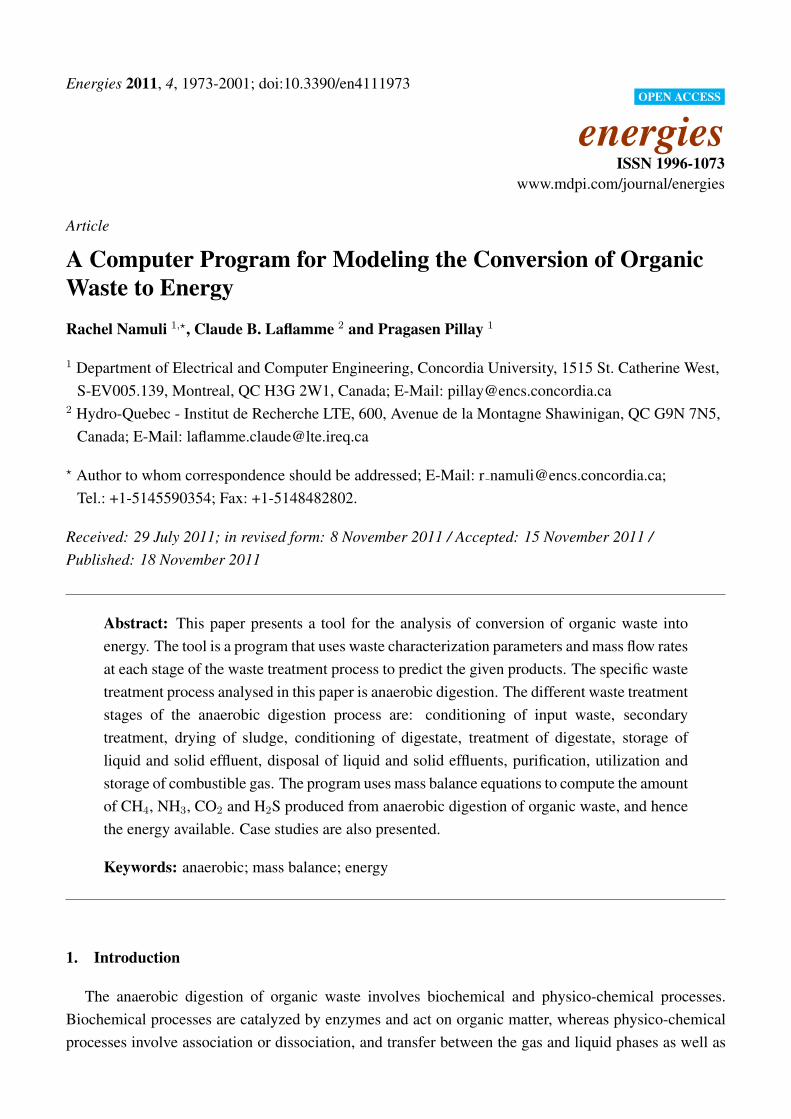
Energies 2011, 4, 1973-2001; doi:10.3390/en4111973OPEN ACCESS

energiesISSN 1996-1073

www.mdpi.com/journal/energies

Article

A Computer Program for Modeling the Conversion of OrganicWaste to EnergyRachel Namuli 1,⋆, Claude B. Laflamme 2 and Pragasen Pillay 1

1 Department of Electrical and Computer Engineering, Concordia University, 1515 St. Catherine West,S-EV005.139, Montreal, QC H3G 2W1, Canada; E-Mail: pillay@encs.concordia.ca

2 Hydro-Quebec - Institut de Recherche LTE, 600, Avenue de la Montagne Shawinigan, QC G9N 7N5,Canada; E-Mail: laflamme.claude@lte.ireq.ca

⋆ Author to whom correspondence should be addressed; E-Mail: r namuli@encs.concordia.ca;Tel.: +1-5145590354; Fax: +1-5148482802.

Received: 29 July 2011; in revised form: 8 November 2011 / Accepted: 15 November 2011 /Published: 18 November 2011

Abstract: This paper presents a tool for the analysis of conversion of organic waste intoenergy. The tool is a program that uses waste characterization parameters and mass flow ratesat each stage of the waste treatment process to predict the given products. The specific wastetreatment process analysed in this paper is anaerobic digestion. The different waste treatmentstages of the anaerobic digestion process are: conditioning of input waste, secondarytreatment, drying of sludge, conditioning of digestate, treatment of digestate, storage ofliquid and solid effluent, disposal of liquid and solid effluents, purification, utilization andstorage of combustible gas. The program uses mass balance equations to compute the amountof CH4, NH3, CO2 and H2S produced from anaerobic digestion of organic waste, and hencethe energy available. Case studies are also presented.

Keywords: anaerobic; mass balance; energy

1. Introduction

The anaerobic digestion of organic waste involves biochemical and physico-chemical processes.Biochemical processes are catalyzed by enzymes and act on organic matter, whereas physico-chemicalprocesses involve association or dissociation, and transfer between the gas and liquid phases as well as

Energies 2011, 4 1974

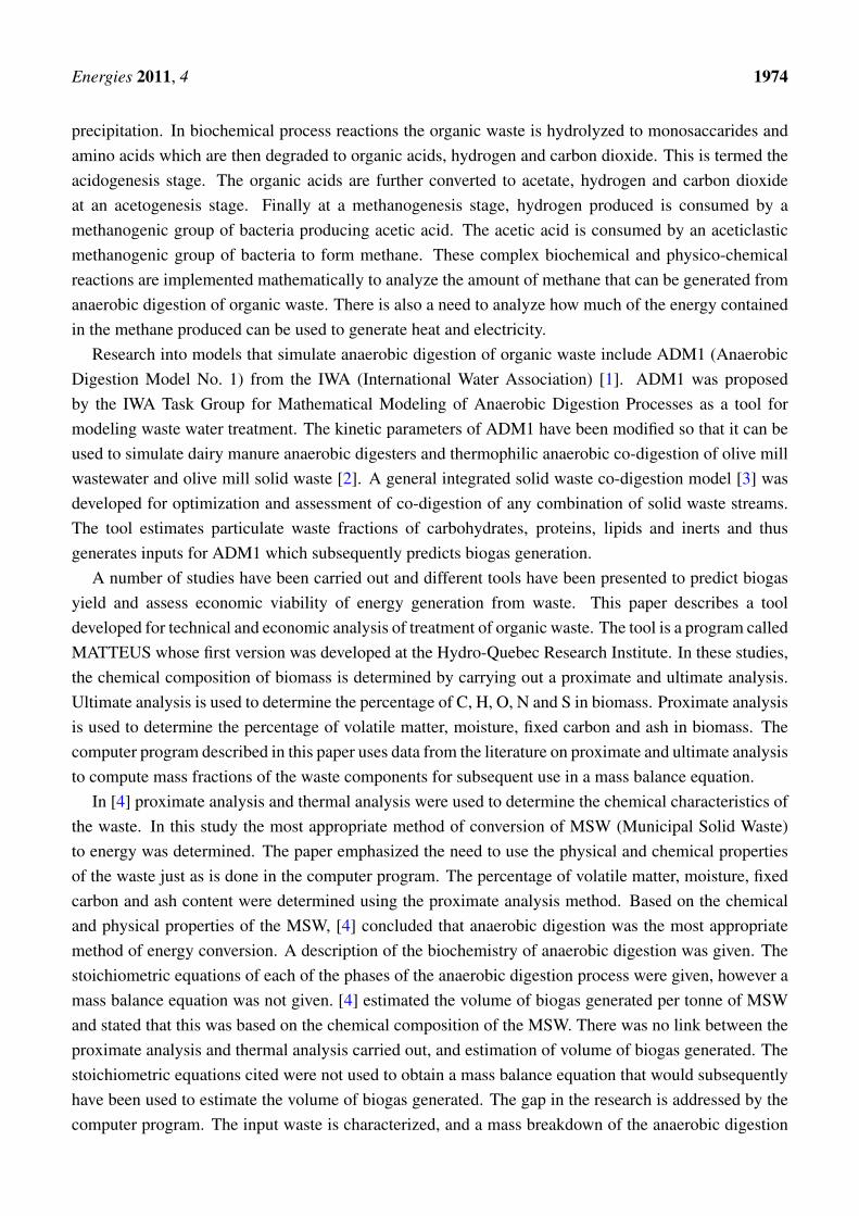
precipitation. In biochemical process reactions the organic waste is hydrolyzed to monosaccarides andamino acids which are then degraded to organic acids, hydrogen and carbon dioxide. This is termed theacidogenesis stage. The organic acids are further converted to acetate, hydrogen and carbon dioxideat an acetogenesis stage. Finally at a methanogenesis stage, hydrogen produced is consumed by amethanogenic group of bacteria producing acetic acid. The acetic acid is consumed by an aceticlasticmethanogenic group of bacteria to form methane. These complex biochemical and physico-chemicalreactions are implemented mathematically to analyze the amount of methane that can be generated fromanaerobic digestion of organic waste. There is also a need to analyze how much of the energy containedin the methane produced can be used to generate heat and electricity.

Research into models that simulate anaerobic digestion of organic waste include ADM1 (AnaerobicDigestion Model No. 1) from the IWA (International Water Association) [1]. ADM1 was proposedby the IWA Task Group for Mathematical Modeling of Anaerobic Digestion Processes as a tool formodeling waste water treatment. The kinetic parameters of ADM1 have been modified so that it can beused to simulate dairy manure anaerobic digesters and thermophilic anaerobic co-digestion of olive millwastewater and olive mill solid waste [2]. A general integrated solid waste co-digestion model [3] wasdeveloped for optimization and assessment of co-digestion of any combination of solid waste streams.The tool estimates particulate waste fractions of carbohydrates, proteins, lipids and inerts and thusgenerates inputs for ADM1 which subsequently predicts biogas generation.

A number of studies have been carried out and different tools have been presented to predict biogasyield and assess economic viability of energy generation from waste. This paper describes a tooldeveloped for technical and economic analysis of treatment of organic waste. The tool is a program calledMATTEUS whose first version was developed at the Hydro-Quebec Research Institute. In these studies,the chemical composition of biomass is determined by carrying out a proximate and ultimate analysis.Ultimate analysis is used to determine the percentage of C, H, O, N and S in biomass. Proximate analysisis used to determine the percentage of volatile matter, moisture, fixed carbon and ash in biomass. Thecomputer program described in this paper uses data from the literature on proximate and ultimate analysisto compute mass fractions of the waste components for subsequent use in a mass balance equation.

In [4] proximate analysis and thermal analysis were used to determine the chemical characteristics ofthe waste. In this study the most appropriate method of conversion of MSW (Municipal Solid Waste)to energy was determined. The paper emphasized the need to use the physical and chemical propertiesof the waste just as is done in the computer program. The percentage of volatile matter, moisture, fixedcarbon and ash content were determined using the proximate analysis method. Based on the chemicaland physical properties of the MSW, [4] concluded that anaerobic digestion was the most appropriatemethod of energy conversion. A description of the biochemistry of anaerobic digestion was given. Thestoichiometric equations of each of the phases of the anaerobic digestion process were given, however amass balance equation was not given. [4] estimated the volume of biogas generated per tonne of MSWand stated that this was based on the chemical composition of the MSW. There was no link between theproximate analysis and thermal analysis carried out, and estimation of volume of biogas generated. Thestoichiometric equations cited were not used to obtain a mass balance equation that would subsequentlyhave been used to estimate the volume of biogas generated. The gap in the research is addressed by thecomputer program. The input waste is characterized, and a mass breakdown of the anaerobic digestion

Energies 2011, 4 1975

process is carried out. This is subsequently used in a mass balance equation to estimate mass flow rateof biogas generated.

In [5] a review of biomass as a fuel for boilers was done. Data from proximate and ultimateanalyses was used to characterize the chemical composition of the biomass, in addition to data fromother analyses. The percentage composition of C, H, O, N, S and Cl for different types of biomasswas determined. [5] shows that proximate and ultimate analysis is an acceptable method of wastecharacterisation. The computer program described in this paper also uses proximate and ultimateanalyses for waste characterisation.

In [6] the potential application of agricultural and animal waste to energy production in Greece wasinvestigated. The study cited the criteria for selection of the method of waste treatment as: the moisturecontent of the input waste, the C/N (Carbon-to-Nitrogen) ratio and physical and chemical characteristicsof the input waste. All these criteria are used in the computer program discussed in this paper. Thecomputer program would thus be a useful tool in the investigation carried out in [6].

In [7] a digester configuration that could be used for anaerobic digestion of grass silage wasinvestigated. The investigation used a mass balance approach similar to that used in the computerprogram. The study also used data from literature on the ultimate analysis of the grass silage. Themass balance equation was derived from the resulting chemical characteristics of the grass silage.

In [8] anaerobic digestion technology for industrial wastewater treatment was studied. In this study,the operating conditions for the anaerobic digestion process were identified as the organic loading rate,temperature, pH and chemical properties of the input waste. Temperature and organic loading rate ofthe anaerobic digestion process are also key operating conditions for the computer program analyzedin this paper. [8] cited the optimal pH range for methane producing bacteria as 6.8–7.2, and an acidicpH for acid forming bacteria. The determination of pH is important to the anaerobic digestion processanalysis. This ensures that the accumulation of VFA (Volatile Fatty Acids) is monitored. The computerprogram however does not compute pH at the various stages of the waste treatment process. [9] estimatedthe methane yield from characteristics of input waste, total solid content in volatile solids and volatilesolids content. Batch tests were carried out on different substrates to determine these parameters, andthe methane yield was estimated. This differs from the approach of the computer program which givesthe detailed formulation of the mass balance equation used to estimate methane yield.

In [10] India’s biogas generation potential from anaerobic digestion of organic waste was assessed.The study obtained data on the amount of waste generated and characterized this into compostable andinert material. Based on studies carried out on the rate of biogas generation from solid waste [10],the biogas potential was estimated. Waste was generalized as MSW, crop residue and agriculturalwaste, animal manure, wastewater and industrial waste. The chemical characteristics of each type ofwaste were not taken into consideration. The computer program improves on such an assessment. Ituses the chemical characteristics of the different types of waste, together with the operating conditionsof the anaerobic digestion process, to estimate the biogas yield. [11] presented an overview of biogasproduction in Zimbabwe. [11] characterized the different types of waste as MSW, sewage sludge, animalmanure and crop residue. Data from literature reviewed was extrapolated to estimate biogas generationpotential from these types of waste. Use of the computer program presented in this paper would givebetter estimates of the biogas generation potential. Similarly in [12], methods for evaluation of renewable

Energies 2011, 4 1976

energy sources were outlined. For the evaluation of energy yield from wet biomass, the author identifiedbiogas yield as being dependent on the physical and chemical composition of the waste. This study alsoused experimental data from literature. Biogas yield was obtained by multiplying the mass of input wasteby a waste availability factor, percentage of dry matter in the waste and the rate of biogas generation perunit of the substrate. Characterization of the waste in study [12] was better than that of [10] and [11],in that it specified dry matter content, organic matter content, percentage of total nitrogen, percentage ofP2O5, percentage of K2O and C/N ratio. The computer program presented in this paper would howeverstill give better estimations of biogas yield since it makes use of a number of physical and chemicalcharacteristics of the waste.

The waste treatment processes of the computer program discussed in this paper are laid out inmodules. A similar approach was used in [9], where an investment decision tool for biogas productionfrom agricultural waste was presented. The paper modeled the anaerobic digestion waste treatmentprocess as a four module process for three different types of feedstock. These processes includedpre-treatment of waste, anaerobic digestion, gas treatment and solids treatment. These waste treatmentprocesses are similar to those of the computer program. The gas treatment process involved biogascleaning and utilization in an internal combustion engine or flaring of the biogas. The computerprogram offers additional options for utilization of the biogas namely; a boiler, a gas turbine and a gasabsorption refrigeration system. Both study [9] and the computer program use mechanical dehydrationfor the solids treatment process. In [9] liquid effluent is treated by evaporation or reverse osmosis,or is used for irrigation. The computer program however offers more options for liquid effluenttreatment, which include ultraviolet radiation, ultraviolet peroxidation, ozonisation, biofiltration andactive carbon filtering.

The computer program carries out an economic analysis of the waste treatment processes. Similarwork has been done in this area in a number of studies and comparisons of the depth of analysis can bemade. In [9] an investment decision tool for biogas production from agricultural waste was presented.There is a significant difference in the economic analysis carried out in [9] and that carried out in thecomputer program. In the former, a financial evaluation was carried out to check the viability of theprocess. The financial evaluation included a calculation of IRR (Internal Rate of Return), NPV (NetPresent Value) and payback period. The computer program however computes avoided costs of sendingthe waste to a landfill, and revenue from sales of products of the waste treatment process.

In [13] a technical and economic evaluation of a biogas based water pumping system is carried outin order to assess its viability. [13] also predicts the potential reduction in CO2 emissions as a result ofusing biogas. This aspect of the analysis is similar to that of the computer program. The savings fromnot using fertilizers were however not quantified by study [13]. [13] however carried out an economicassessment based on NPV, benefit to cost ratio and IRR. This depth of economic analysis is not done inthe computer program described in this paper.

The rest of the paper describes the computer program and is organized as follows: Section 2 is adescription of the program, Section 3 explains the mathematical modeling of the process, Section 4explains the determination of heat generated by boilers, Section 5 gives energy conversion efficienciesof spark ignition engines, Section 6 explains the method of economic analysis and Section 7 gives casestudies to which the program is applied.

Energies 2011, 4 1977

2. Description of the Program

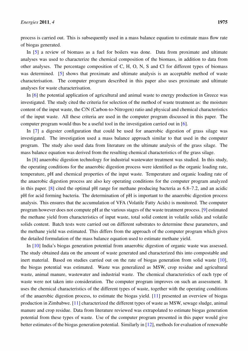
The main feature of the program is characterization and analysis of input waste, waste flow streamsand by-products of waste processing. Physical properties and volume flow rates of the waste streamsare computed. The program analyses conditioning of input waste, primary waste treatment, secondarywaste treatment and handling of by-products. An economic analysis of the waste treatment methods isalso done.

The various waste treatment stages of the program are laid out in modules. The process flow frominputs to production of energy and disposal of final products is shown in Figure 1.

Figure 1. The program’s computation procedure.

Energies 2011, 4 1978

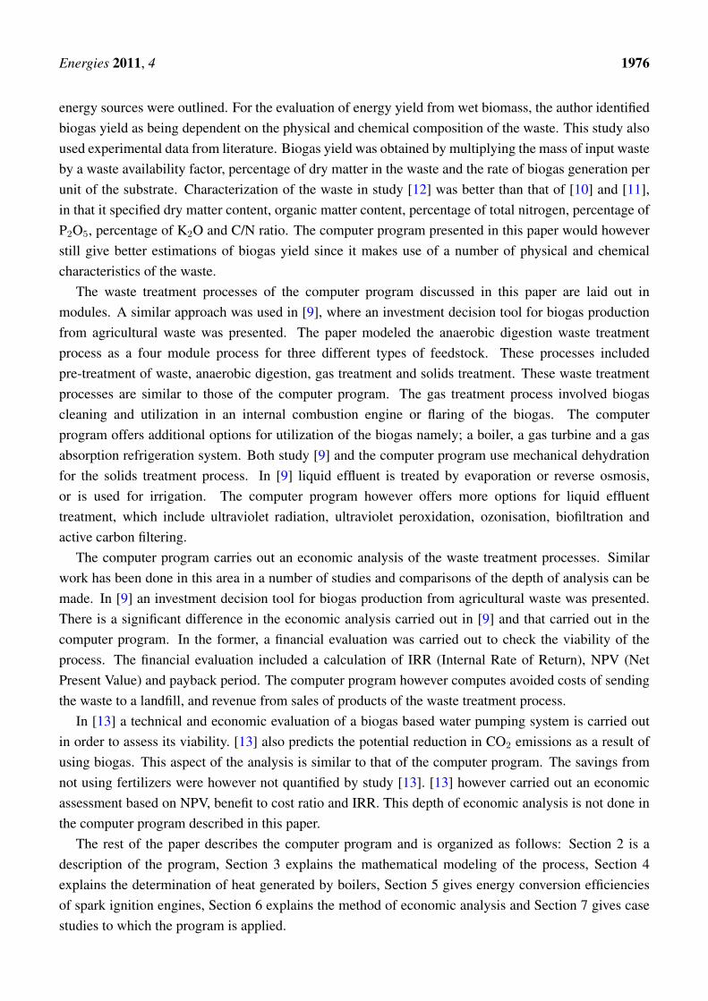
The type of waste to be treated has to be characterized by parameters given in Table 1. The programhas a database of mass fractions for the different classifications of waste based on a literature reviewof ultimate and proximate analysis of the types of waste. Users can choose to use the parameters fromthe database or to enter their own parameters from a literature review of ultimate or proximate analysis.Although provision has been made for entry of pH, it is not used in computations in the worksheet. Thiswill be included in future versions of the program.

Table 1. Input parameters for waste characterization.

Parameter Description

Density (tmh/m3) densityDryness (tms/tmh)C (t/tms) organic CarbonH (t/tms) organic HydrogenO (t/tms) organic OxygenN (t/tms) organic Nitrogen in ammoniaS (t/tms) organic SulphurAshes (t/tms) inorganic matterP2O5 (t/tms) phosphorus; included in the ashesK2O (t/tms) potassium; included in the ashesSoluble organic VS (t/tVS) soluble organic volatile solidsSoluble MI (t/tmi) soluble inorganic matterP soluble (t/tP) soluble PhosphorusK soluble (t/tK) soluble PotassiumDistance (km) distance to treatment siteCost of waste disposal ($/tms) avoided cost of waste disposal

The program requires definition and entry of operating conditions and economic parameters for thevarious waste treatment stages. The user is required to define mass flow rates of input waste, physicalproperties of waste, hydraulic retention time, elimination of volatile solids, equipment costs, operationaland maintenance costs, transportation, energy required, utilization rates, site conditions, global warmingfactors, costs scaling factors and capital costs. Section 3 on mathematical modeling of the processesdescribes how the operating conditions and economic parameters are obtained. The program does notcompute precipitation of phosphorus during the waste treatment process.

3. Mathematical Modeling of the Process

Section 3 is on the technical analysis of the waste treatment process and outlines equations used. Onlythe anaerobic digestion process will be analyzed, based on mass balance of the organic matter. Mass flowrates are computed for each waste treatment stage. The procedure for analysis of the waste treatmentprocess involves sequential analysis of the mass flow rates, physical properties of the treated waste andproducts, through the various waste treatment stages. An economic analysis of the process is also carried

Energies 2011, 4 1979

out based on required capacity. Required capacity is estimated from the mass balance analysis carriedout. Mass balance equations used to compute breakdown of organic matter are given. Equations forcomputation of physical properties like generation of heat, density, LCV (Lower Calorific Value), HCV(Higher Calorific Value), reaction rates and dryness are given.

3.1. Dryness of Matter

The dryness of input waste is computed as it is one of the properties used to characterize waste flow.Dryness of matter ωms is the content of dry matter in wet matter and is computed using Equation (1).

ωms =mms

mmh(1)

where mms is the mass of dry matter and mmh is the mass of wet matter.

3.2. Calorific Values of Input Waste

LCV and HCV of input organic matter are required to compute energy released from the reactions ina digester. These are computed using Equations (2) and (3) respectively in GJ/tms [14]. The mass fractionof dry weight over wet weight is used to compute the calorific values. Mass fractions of dry weight areused instead of mass of wet weight. This is because Equations (2) and (3) are formulated by curve fittingof experimental data from ultimate analysis, where ultimate analysis gives the composition of the inputmatter in terms of dry mass for C, H, O, S and N.

HCV = 34.91ωC + 117.83ωH − 10.34ωO − 1.51ωN + 10.05ωS − 2.11ωashes [GJ/t] (2)

LCV = HCV − 22.36ωH [GJ/t] (3)

where ωC, ωH, ωO, ωN, ωS and ωashes are mass fractions of C, H, O, N, S and ashes respectively, in theinput waste.

Equation (2) can generate negative values (which is incorrect) if the content of inorganic matter inthe waste is more significant than the content of organic matter in the waste. In this case, Equation (2)is used without the term for mass fraction of ashes in the waste, and thus the equations are modified toEquations (4) and (5).

HCV = 34.91ωC + 117.83ωH − 10.34ωO − 1.51ωN + 10.05ωS [GJ/t] (4)

LCV = HCV − 22.36ωH [GJ/t] (5)

where ωC, ωH, ωO, ωN and ωS are mass fractions on a dry basis of C, H, O, N and S respectively, containedin the volatile solids of the input waste.

If the user provides data on mass fractions of the waste components, LCV and HCV are correctedusing Equations (6) and (7) respectively.

LCV = LCVref(1 − ωashes)

(1 − ωashes,ref)[GJ/t] (6)

HCV = HCVref(1 − ωashes)

(1 − ωashes,ref)[GJ/t] (7)

Energies 2011, 4 1980

where LCV is the lower calorific value of the components entered by the user, LCVref is the lowercalorific value of the input reference from the program’s database, HCV is the higher calorific value ofthe components entered by the user and HCVref is the higher calorific value of the input reference fromthe program’s database.

3.3. Density of Input Waste

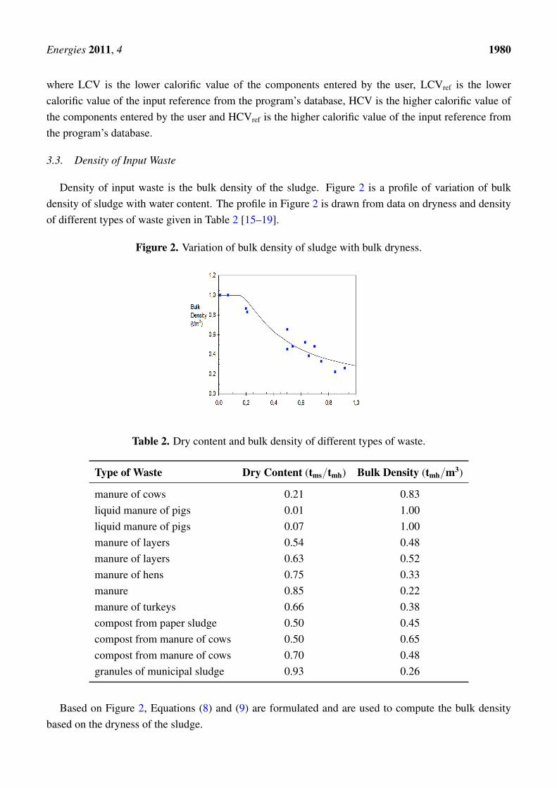
Density of input waste is the bulk density of the sludge. Figure 2 is a profile of variation of bulkdensity of sludge with water content. The profile in Figure 2 is drawn from data on dryness and densityof different types of waste given in Table 2 [15–19].

Figure 2. Variation of bulk density of sludge with bulk dryness.

Table 2. Dry content and bulk density of different types of waste.

Type of Waste Dry Content (tms/tmh) Bulk Density (tmh/m3)

manure of cows 0.21 0.83liquid manure of pigs 0.01 1.00liquid manure of pigs 0.07 1.00manure of layers 0.54 0.48manure of layers 0.63 0.52manure of hens 0.75 0.33manure 0.85 0.22manure of turkeys 0.66 0.38compost from paper sludge 0.50 0.45compost from manure of cows 0.50 0.65compost from manure of cows 0.70 0.48granules of municipal sludge 0.93 0.26

Based on Figure 2, Equations (8) and (9) are formulated and are used to compute the bulk densitybased on the dryness of the sludge.

Energies 2011, 4 1981

ρb = 1.0 for ϕb ≤ 0.15 [t/m3] (8)

ρb = 1.0 − exp

[−0.3

ϕb − 0.1

]for ϕb > 0.15 [t/m3] (9)

where ρb is bulk density of the waste and ϕb is dry content of the waste.

3.4. Volume Throughput of Waste

The program works with mass throughput in the computation of the waste flow through the treatmentstages. However some waste treatment stages like transport, secondary treatment and storage, workwith volume throughput. Therefore Equation (10) is used to compute volume throughput using massthroughput and bulk density of the sludge.

V =mmh

ρb[m3/h] (10)

where V is volume flow rate and mmh is mass flow rate on a wet basis.

3.5. Volume Throughput of Biogas

Volume throughput of the biogas is computed from the mass flow rates and densities of thecomponents of the biogas. The density of a component of the biogas ρi at a given temperature andpressure is computed based on the perfect gas law Equation (11).

ρi =piMi

RT[t/m3] (11)

where pi is the partial pressure of the gas component, Mi is the molecular mass of the gas component, R

is the universal perfect gas constant and T is the temperature of the gas in Kelvin.Thus the volume flow rate of each of the biogas components Vi is computed using Equation (12).

Vi =miRT

piMi

[m3/h] (12)

where mi is the mass flow rate of the gas component.The sum of the volume throughputs of the components of the biogas will give the volume throughput

of the biogas.

3.6. Total Throughput of Properties of the Waste

Total throughput of properties of the waste is required in the waste analysis, for example forformulation of the mass balance equation Equations (20) and (21). Each stage of the waste treatmentprocess generates partial mass throughputs as well as partial calorific values of the waste components.The total throughput and total calorific value are then obtained by summing the partial throughputsEquation (13).

xk,n =n∑

i=1

xk,i [t/h] (13)

Energies 2011, 4 1982

where xk,n is the total mass throughput or calorific value of matter i with n components. k is therespective property, i.e., mass throughput, HCV or LCV.

Total volume throughput of the matter i cannot be obtained from the sum of the partial volumethroughputs of its components since the components do not have the same density, as seen in Section 3.5.Volume flow rate of biogas is obtained from the mass and density of its components, not from summationof volume throughputs of its components. Total volume throughput of the matter i is thus computed usingEquation (12).

3.7. Temperature and Pressure of Waste

The various stages of waste treatment also require values of temperature and pressure of inputs andoutputs. If the temperature and pressure of a given waste treatment stage affects the temperature andpressure of the following treatment stage (this applies when there is energy transfer without delay),the temperature and pressure of the latter are computed by a weighted average of the respective massthroughputs as expressed in Equation (14).

xn =

∑ni=1 mixi

mm[◦C or atm] (14)

where xn is the temperature or pressure of the waste, mi is the mass throughput of the waste componenti, xi is the temperature or pressure of the waste component i and mm is the mass throughput of the wasteat the previous treatment stage.

If the temperature and pressure of the waste treatment stage does not impact the temperatureand pressure of the following waste treatment stage, the program uses default values contained inthe worksheet.

The following sections give mass balance equations that are used by the program to analyse theformation of biogas and new biomass from anaerobic digestion of organic waste. Computation ofparameters that determine the operating conditions of the anaerobic digestion process is also included.These conditions include organic loading rate, dilution of digester effluent, heat losses from the digesterand heat of reaction of the effluent in the digester.

3.8. Organic Loading Rate

Organic loading rate is expressed as COD, i.e., the mass of oxygen required to entirely oxidize thecompounds contained in the digester effluent. Organic loading rate is computed using Equation (15).

mCOD

mms= 31.99

[α

12.01+

β

4(1.01)− γ

2(15.99+

ε

32.06

][kgVS/m3/day] (15)

where mCOD is the mass of oxygen required for the oxidization, mms is the mass of dry matter, and α, β,γ, δ and ε are mass fractions of biomass of composition CαHβOγNδSε.

Nitrogen is considered inert and thus formation of nitrogen oxides is neglected. The nitrogencomponent is not included in Equation (15).

Energies 2011, 4 1983

3.9. Digester Operating Temperature

The user of the model specifies the operating temperature of the digester. There is an option forthermophilic, mesophilic or psychrophilic temperatures. The thermophilic temperature is set to 55 ◦C,the mesophilic temperature is set to 35 ◦C and the psychrophilic temperature is set to 20 ◦C. It is assumedthat the operating temperature of the digester is kept constant throughout the year by heating the digester.

3.10. Dilution of Digester Effluent

Digester effluent may be diluted to reduce dryness or toxicity. The anaerobic digester modulecomputes dryness and toxicity of nitrogen in the effluent, in order to compare the values achieved withmaximum values set. This impacts on the economic analysis since it involves addition of water to theeffluent. Equation (16) computes the desired dryness of digester effluent.

ϕ1+2 =m1ϕ1

m1 + m2

(16)

where ϕ1+2 is desired dryness of the digester effluent, m1 is mass throughput of wet matter, ϕ1 is drynessof matter before addition of water and m2 is mass of water added.

If the desired dryness of the digester effluent is known and the amount of water to be added is required,Equation (17) is used.

m2 =m1(ϕ1 − ϕ1+2)

ϕ1+2

[t/h] (17)

3.11. Heat of Reaction of Effluent

Elimination of the COD by anaerobic digestion results in generation or absorption of heat in thedigester effluent, depending on the nature of the organic material. Estimation of the net heat generatedis calculated by HCVbefore − HCVafter, using Equation (4).

3.12. Rate of Elimination of Volatile Solids

The anaerobic digester’s performance is characterized by effectiveness of elimination of total volatilesolids, ηVSt. This is separated into mass breakdown of dissolved volatile solids and non-dissolved volatilesolids. The effectiveness of elimination of dissolved volatile solids, ηDVS, is higher than the effectivenessof elimination of non-dissolved volatile solids, ηNDVS. Based on the respective masses of the componentsof the input, partial effectiveness of elimination of dissolved volatile solids and partial effectiveness ofelimination of non-dissolved volatile solids are computed separately and are used in Equation (18) todefine the effectiveness of elimination of total volatile solids.

ηVStmVSt = ηDVSmDVS + ηNDV SmNDVS (18)

where ηVSt is the effectiveness of elimination of total volatile solids, mVSt is the mass of total volatilesolids, ηDVS is effectiveness of elimination of dissolved volatile solids, mDVS is the mass of dissolvedvolatile solids, ηNDVS is effectiveness of elimination of non-dissolved volatile solids and mNDVS is themass of non-dissolved volatile solids.

Energies 2011, 4 1984

The program uses a rate of elimination of dissolved and non-dissolved volatile solids of 95% and40% respectively, at 37 ◦C for a hydraulic retention time of 25 days. Equation (18) and a typical rateof elimination of total volatile solids of 60% is used to estimate the rate of elimination of non-dissolvedvolatile solids. The value 60% is obtained from liquid manure of pigs containing typically 37% ofnon-soluble volatile solids. This is confirmed with the rates of biological breakdown measured by [20],for papers and carton whose mDVS = 0.

3.13. Limits of Reaction by C/N Ratio

The mixture of inputs to the anaerobic digestion process should ideally have a C/N ratio of between20 and 40 to allow a balanced growth of micro-organisms. The program computes the C/N ratio of themixture of inputs and sends an error message if the C/N ratio exceeds 40. It will nevertheless carryon with the process analysis. The effective C/N ratio is computed using Equation (19) that considersthe total carbon available to the anaerobic digestion process, and the total nitrogen in the dissolvedand non-dissolved matter. Organic carbon that is non-biodegradable such as lignin is not considered inEquation (19) because it is considered biologically inert.

C

N|eff =

mC-biodegradable

mN-total(19)

where CN|eff is the effective carbon to nitrogen ratio in the mixture of inputs, mC-biodegradable, is the total

carbon available to the anaerobic digestion process and mN-total is the total nitrogen in the dissolved andnon-dissolved matter.

3.14. Dilution to Control Dryness and Toxicity

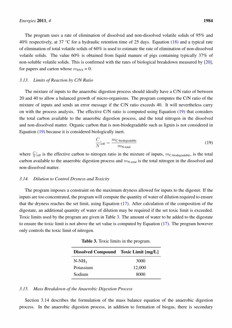
The program imposes a constraint on the maximum dryness allowed for inputs to the digester. If theinputs are too concentrated, the program will compute the quantity of water of dilution required to ensurethat the dryness reaches the set limit, using Equation (17). After calculation of the composition of thedigestate, an additional quantity of water of dilution may be required if the set toxic limit is exceeded.Toxic limits used by the program are given in Table 3. The amount of water to be added to the digestateto ensure the toxic limit is not above the set value is computed by Equation (17). The program howeveronly controls the toxic limit of nitrogen.

Table 3. Toxic limits in the program.

Dissolved Compound Toxic Limit [mg/L]

N-NH3 3000Potassium 12,000Sodium 8000

3.15. Mass Breakdown of the Anaerobic Digestion Process

Section 3.14 describes the formulation of the mass balance equation of the anaerobic digestionprocess. In the anaerobic digestion process, in addition to formation of biogas, there is secondary

Energies 2011, 4 1985

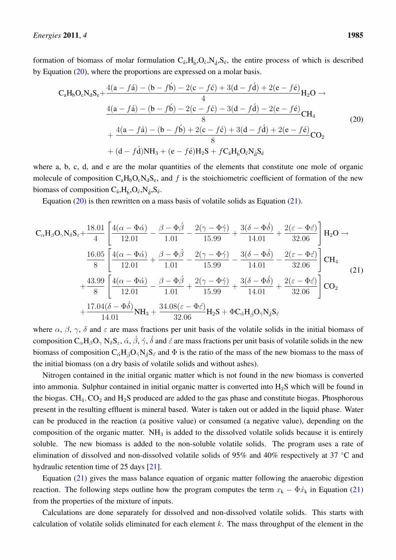
formation of biomass of molar formulation Ca,Hb,Oc,Nd,Se, the entire process of which is describedby Equation (20), where the proportions are expressed on a molar basis.

CaHbOcNdSe+4(a − f a) − (b − f b) − 2(c − f c) + 3(d − f d) + 2(e − f e)

4H2O →

4(a − f a) − (b − f b) − 2(c − f c) − 3(d − f d) − 2(e − f e)8

CH4

+4(a − f a) − (b − f b) + 2(c − f c) + 3(d − f d) + 2(e − f e)

8CO2

+ (d − f d)NH3 + (e − f e)H2S + fCaHbOcNdSe

(20)

where a, b, c, d, and e are the molar quantities of the elements that constitute one mole of organicmolecule of composition CaHbOcNdSe, and f is the stoichiometric coefficient of formation of the newbiomass of composition Ca,Hb,Oc,Nd,Se.

Equation (20) is then rewritten on a mass basis of volatile solids as Equation (21).

CαHβOγNδSε+18.01

4

[4(α − Φα)

12.01− β − Φβ

1.01− 2(γ − Φγ)

15.99+

3(δ − Φδ)

14.01+

2(ε − Φε)

32.06

]H2O →

16.05

8

[4(α − Φα)

12.01+

β − Φβ

1.01− 2(γ − Φγ)

15.99− 3(δ − Φδ)

14.01− 2(ε − Φε)

32.06

]CH4

+43.99

8

[4(α − Φα)

12.01− β − Φβ

1.01+

2(γ − Φγ)

15.99+

3(δ − Φδ)

14.01+

2(ε − Φε)

32.06

]CO2

+17.04(δ − Φδ)

14.01NH3 +

34.08(ε − Φε)

32.06H2S + ΦCαHβOγNδSε

(21)

where α, β, γ, δ and ε are mass fractions per unit basis of the volatile solids in the initial biomass ofcomposition CαHβOγ NδSε, α, β, γ, δ and ε are mass fractions per unit basis of volatile solids in the newbiomass of composition CαHβOγNδSε and Φ is the ratio of the mass of the new biomass to the mass ofthe initial biomass (on a dry basis of volatile solids and without ashes).

Nitrogen contained in the initial organic matter which is not found in the new biomass is convertedinto ammonia. Sulphur contained in initial organic matter is converted into H2S which will be found inthe biogas. CH4, CO2 and H2S produced are added to the gas phase and constitute biogas. Phosphorouspresent in the resulting effluent is mineral based. Water is taken out or added in the liquid phase. Watercan be produced in the reaction (a positive value) or consumed (a negative value), depending on thecomposition of the organic matter. NH3 is added to the dissolved volatile solids because it is entirelysoluble. The new biomass is added to the non-soluble volatile solids. The program uses a rate ofelimination of dissolved and non-dissolved volatile solids of 95% and 40% respectively at 37 ◦C andhydraulic retention time of 25 days [21].

Equation (21) gives the mass balance equation of organic matter following the anaerobic digestionreaction. The following steps outline how the program computes the term xk − Φxk in Equation (21)from the properties of the mixture of inputs.

Calculations are done separately for dissolved and non-dissolved volatile solids. This starts withcalculation of volatile solids eliminated for each element k. The mass throughput of the element in the

Energies 2011, 4 1986

initial volatile solid, mk,o, in the phase considered, and the rate of removal of volatile solid ηel is used inEquation (22).

mk,el = mk,oηe,l [t/h] (22)

where mk,el is the mass of volatile solids eliminated for each element k.The mass throughput of the volatile solids eliminated in the phase considered is obtained by the sum

of the partial mass throughputs of the elements that constitute the input. It is calculated by Equation (23).

mVS,el =n∑

k=1

mk,el [t/h] (23)

where mVS,el is the mass throughput of the volatile solids eliminated.Equation (24) is then used to calculate the mass throughput of the new biomass which appears at

a rate Φ. Φ is defined as the ratio of the mass of the new biomass to the mass of the initial biomass(on a dry basis of volatile solids and without ashes). The program uses a default value for Φ of0.04 tms/tCODeliminated [22].

mVS,b = ΦmVS,el [t/h] (24)

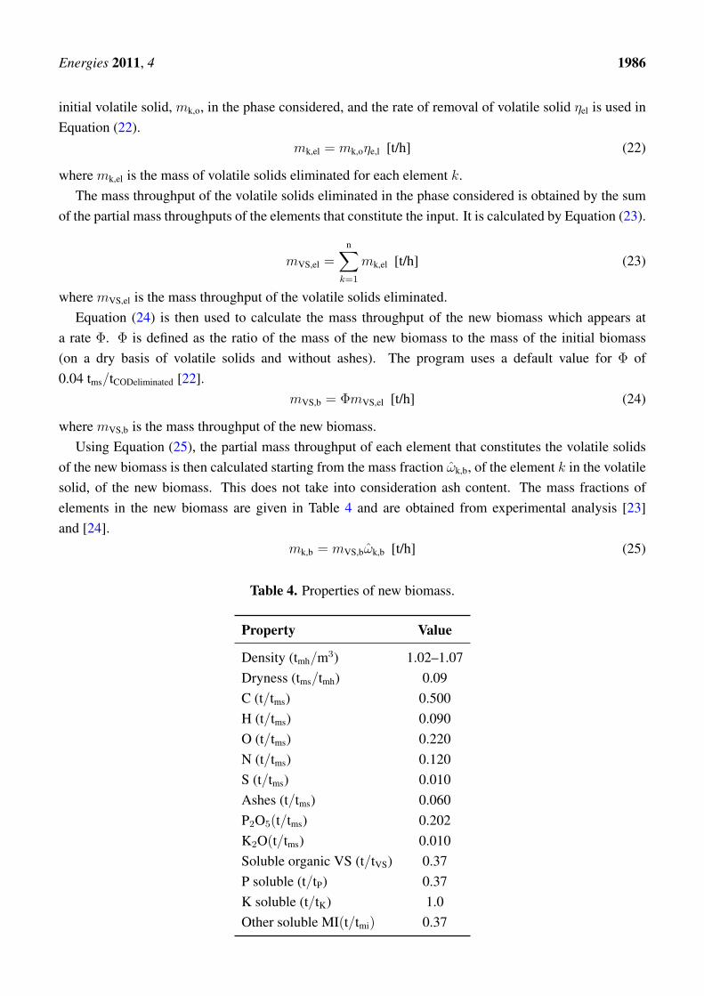
where mVS,b is the mass throughput of the new biomass.Using Equation (25), the partial mass throughput of each element that constitutes the volatile solids

of the new biomass is then calculated starting from the mass fraction ωk,b, of the element k in the volatilesolid, of the new biomass. This does not take into consideration ash content. The mass fractions ofelements in the new biomass are given in Table 4 and are obtained from experimental analysis [23]and [24].

mk,b = mVS,bωk,b [t/h] (25)

Table 4. Properties of new biomass.

Property Value

Density (tmh/m3) 1.02–1.07Dryness (tms/tmh) 0.09C (t/tms) 0.500H (t/tms) 0.090O (t/tms) 0.220N (t/tms) 0.120S (t/tms) 0.010Ashes (t/tms) 0.060P2O5(t/tms) 0.202K2O(t/tms) 0.010Soluble organic VS (t/tVS) 0.37P soluble (t/tP) 0.37K soluble (t/tK) 1.0Other soluble MI(t/tmi) 0.37

Energies 2011, 4 1987

The mass throughput of each by-product is thus given by Equation (21), in which the term xk − Φxk

is given by Equation (26), which is obtained from Equations (22)–(25).

xk − Φxk = mk,el − mk,b [t/h] (26)

4. Heat Generation by Boilers

The program defines the exhaust temperature of boilers of given capacity based on data given inTable 5. Table 5 gives the stoichiometric ratios of air and the temperatures of exhaust gases. Thestoichiometric ratio of air and temperatures of exhaust gases of the respective boiler capacities is what isused to estimate heat production from combustion of gases in a boiler.

Table 5. Exhaust temperatures for biogas boilers of different capacities.

Parameter Value

Energy of evaporation <3 MW 3–6 MW 6–19 MW >19 MWStoichiometric ratio of air 1.2–1.3 1.2–1.3 1.15–1.3 1.1–1.2Exhaust gas temperature 220 ◦C 200 ◦C 170 ◦C 170 ◦C

Source: Japan Energy Conservation Handbook 2005/2006 [25].

5. Spark Ignition Engine Generator Set

The efficiency of energy conversion is used to compute the amount of electricity generated for agiven rating of a spark ignition engine-generator set. The program estimates the efficiency of energyconversion based on linear interpolation using Equation (27).

ηe = (0.36 − 0.28)

[log Pe − log(20)

log(1000) − log(20)

]+ 0.28 for 20 ≤ Pe ≤ 5000 [kWe] (27)

where ηe is the efficiency of energy conversion and Pe is the electrical power output.If exhaust heat is recovered, total CHP efficiency in relation to LCV is given in Table 6 [26] for

different spark ignition engine ratings. The total CHP efficiency in turn is used to estimate electricityand heat production for a CHP system.

Table 6. CHP efficiencies of spark ignition engine generator sets.

Parameter Value

Reference Capacity (kWe) 100 300 1000 3000 5000Total CHP efficiency (%) 78 77 71 69 73

Source: Golstein et al. [26].

6. Economic Analysis

Section 6 gives equations used to carry out the economic analysis of the waste treatment process.

Energies 2011, 4 1988

6.1. Scaling Parameter

The program uses reference capital costs Cref which are published values compared to a given capacity(referred to as capacity of reference Qref). There is a relationship between the cost of a unit ofequipment and its capacity. If this cost is plotted against the capacity on a logarithmic scale, the best fitcurve obtained is a straight line. The equation of the line is obtained as Equation (28) [27]. This equationis used to estimate the capital costs C1 of the desired or required capacity Q1.

C1 = Cref

[Q1

Qref

]v

[$] (28)

where v is a scaling parameter. The program uses a default scaling parameter of 0.6. The value of thescaling parameter is generally in the interval 0 ≤ v ≤ 1. The most frequently used value is 0.6 [27].

The economic analysis requires computation of total reference capacity cost that is given byEquation (29).

Ctotal ref = Cref 1(1 + Cinstallation + Ceng admin) [$] (29)

where Ctotal ref is the total reference capacity cost, Cref 1 is the reference investment cost, Cinstallation is theinstallation cost and Ceng admin is the cost of engineering and administration.

6.2. Operation and Maintenance Costs

The program sets the annual operational and maintenance costs to 5% of equipment costs by default(excluding the energy costs). If however the specific operational and maintenance cost Cref is knownfor a given reference capacity Qref, the operational and maintenance cost C1 for another capacity Q1 canbe extrapolated using Equation (30).

C1Q1 = CrefQref

[Q1

Qref

]v

[$] (30)

where v is the scaling parameter set to 0.6 [27].Specific costs of energy are not scaled down as they remain the same as those of the reference capacity,

since they apply to unit cost of the treatment capacity or energy production.The digester capacity is computed from the volume flow rate of input waste and the hydraulic retention

time using:Qdigester = 24V HRT [m3] (31)

where Qdigester is the capacity of the digester, V is the volume flow rate of input waste in m3/h and HRTis the hydraulic retention time in days.

7. Comparison of the Computer Program’s Predictions with Results from Case Studies

The previous sections described the computer program for organic waste analysis. This sectioncompares predictions of the computer program with actual biogas yields and biogas composition. Twocase studies have been looked at, A.A. Dairy farm [28] and Noblehurst Dairy farm [29]. Ultimate andproximate analysis data of the case studies was unavailable, hence ultimate analysis data was derived

Energies 2011, 4 1989

using a transformation matrix [30]. Proximate analysis data available in the computer program’s databasewas used.

This section describes a transformation matrix that has been used to estimate ultimate analysis data.It also gives the digesters’ operating conditions.

7.1. Transformation Matrix

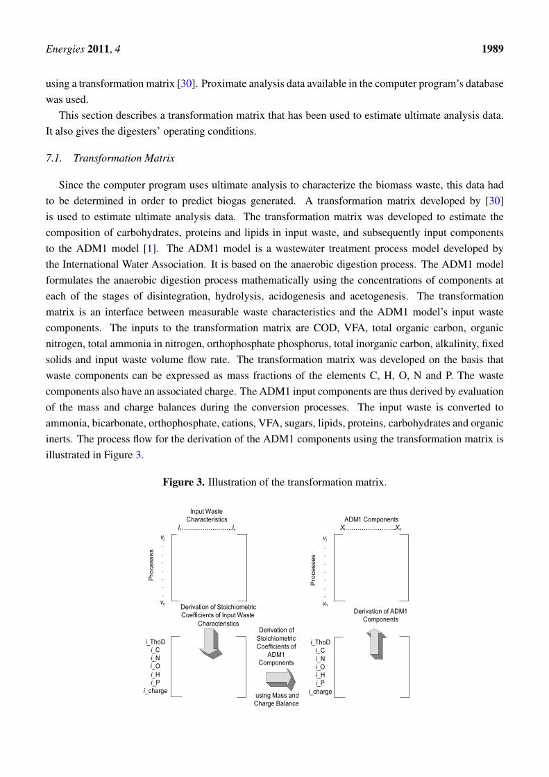
Since the computer program uses ultimate analysis to characterize the biomass waste, this data hadto be determined in order to predict biogas generated. A transformation matrix developed by [30]is used to estimate ultimate analysis data. The transformation matrix was developed to estimate thecomposition of carbohydrates, proteins and lipids in input waste, and subsequently input componentsto the ADM1 model [1]. The ADM1 model is a wastewater treatment process model developed bythe International Water Association. It is based on the anaerobic digestion process. The ADM1 modelformulates the anaerobic digestion process mathematically using the concentrations of components ateach of the stages of disintegration, hydrolysis, acidogenesis and acetogenesis. The transformationmatrix is an interface between measurable waste characteristics and the ADM1 model’s input wastecomponents. The inputs to the transformation matrix are COD, VFA, total organic carbon, organicnitrogen, total ammonia in nitrogen, orthophosphate phosphorus, total inorganic carbon, alkalinity, fixedsolids and input waste volume flow rate. The transformation matrix was developed on the basis thatwaste components can be expressed as mass fractions of the elements C, H, O, N and P. The wastecomponents also have an associated charge. The ADM1 input components are thus derived by evaluationof the mass and charge balances during the conversion processes. The input waste is converted toammonia, bicarbonate, orthophosphate, cations, VFA, sugars, lipids, proteins, carbohydrates and organicinerts. The process flow for the derivation of the ADM1 components using the transformation matrix isillustrated in Figure 3.

Figure 3. Illustration of the transformation matrix.

Energies 2011, 4 1990

In Figure 3, v represents a conversion process, I is an input waste characteristic and X is an ADM1component. The stoichiometric coefficients of the theoretical oxygen demand, the elements and chargeare represented by i ThoD, i C, i N, i O, i H, i P and i charge, respectively.

7.2. Estimating Ultimate Analysis Data

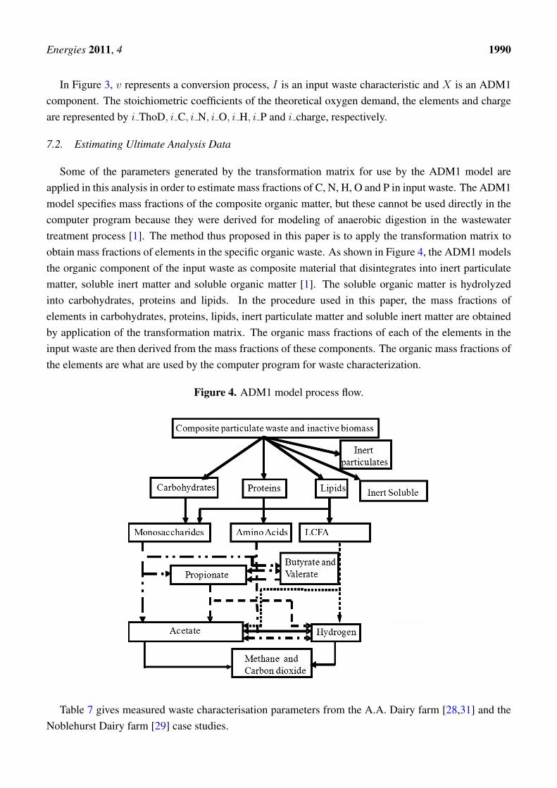
Some of the parameters generated by the transformation matrix for use by the ADM1 model areapplied in this analysis in order to estimate mass fractions of C, N, H, O and P in input waste. The ADM1model specifies mass fractions of the composite organic matter, but these cannot be used directly in thecomputer program because they were derived for modeling of anaerobic digestion in the wastewatertreatment process [1]. The method thus proposed in this paper is to apply the transformation matrix toobtain mass fractions of elements in the specific organic waste. As shown in Figure 4, the ADM1 modelsthe organic component of the input waste as composite material that disintegrates into inert particulatematter, soluble inert matter and soluble organic matter [1]. The soluble organic matter is hydrolyzedinto carbohydrates, proteins and lipids. In the procedure used in this paper, the mass fractions ofelements in carbohydrates, proteins, lipids, inert particulate matter and soluble inert matter are obtainedby application of the transformation matrix. The organic mass fractions of each of the elements in theinput waste are then derived from the mass fractions of these components. The organic mass fractions ofthe elements are what are used by the computer program for waste characterization.

Figure 4. ADM1 model process flow.

Table 7 gives measured waste characterisation parameters from the A.A. Dairy farm [28,31] and theNoblehurst Dairy farm [29] case studies.

Energies 2011, 4 1991

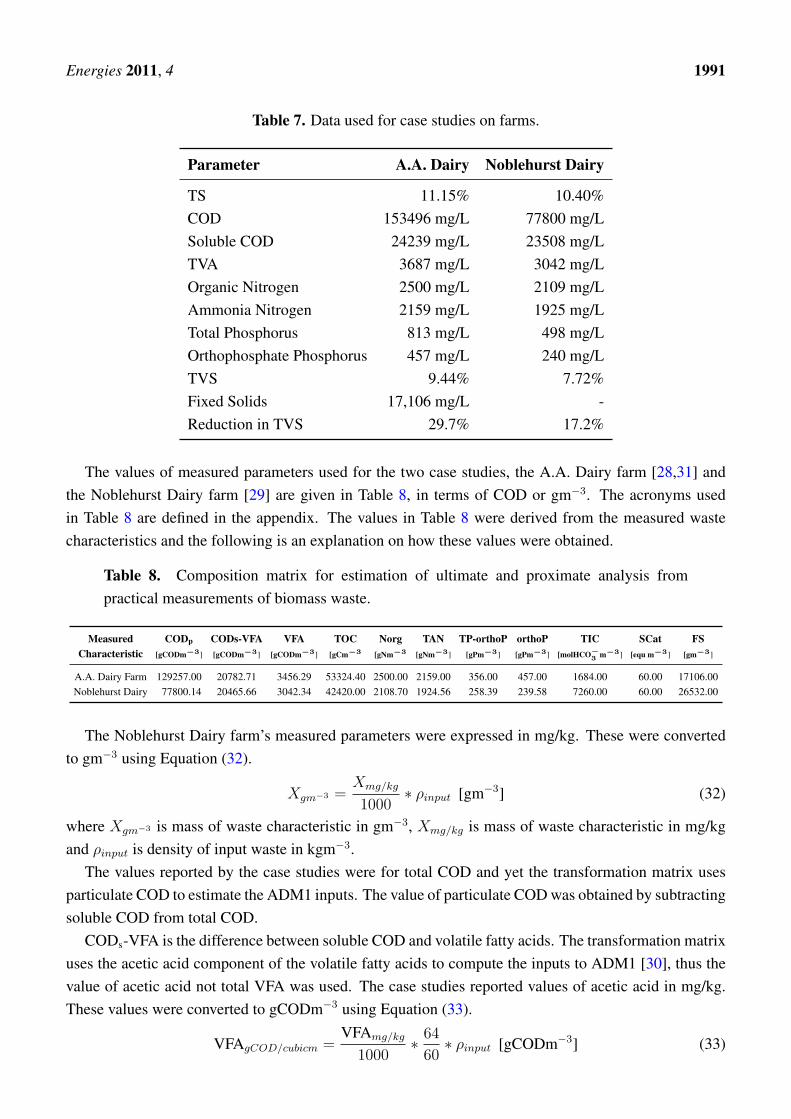
Table 7. Data used for case studies on farms.

Parameter A.A. Dairy Noblehurst Dairy

TS 11.15% 10.40%COD 153496 mg/L 77800 mg/LSoluble COD 24239 mg/L 23508 mg/LTVA 3687 mg/L 3042 mg/LOrganic Nitrogen 2500 mg/L 2109 mg/LAmmonia Nitrogen 2159 mg/L 1925 mg/LTotal Phosphorus 813 mg/L 498 mg/LOrthophosphate Phosphorus 457 mg/L 240 mg/LTVS 9.44% 7.72%Fixed Solids 17,106 mg/L -Reduction in TVS 29.7% 17.2%

The values of measured parameters used for the two case studies, the A.A. Dairy farm [28,31] andthe Noblehurst Dairy farm [29] are given in Table 8, in terms of COD or gm−3. The acronyms usedin Table 8 are defined in the appendix. The values in Table 8 were derived from the measured wastecharacteristics and the following is an explanation on how these values were obtained.

Table 8. Composition matrix for estimation of ultimate and proximate analysis frompractical measurements of biomass waste.

Measured CODp CODs-VFA VFA TOC Norg TAN TP-orthoP orthoP TIC SCat FSCharacteristic [gCODm−3] [gCODm−3] [gCODm−3] [gCm−3 [gNm−3 [gNm−3] [gPm−3] [gPm−3] [molHCO−

3 m−3] [equ m−3] [gm−3]

A.A. Dairy Farm 129257.00 20782.71 3456.29 53324.40 2500.00 2159.00 356.00 457.00 1684.00 60.00 17106.00Noblehurst Dairy 77800.14 20465.66 3042.34 42420.00 2108.70 1924.56 258.39 239.58 7260.00 60.00 26532.00

The Noblehurst Dairy farm’s measured parameters were expressed in mg/kg. These were convertedto gm−3 using Equation (32).

Xgm−3 =Xmg/kg

1000∗ ρinput [gm−3] (32)

where Xgm−3 is mass of waste characteristic in gm−3, Xmg/kg is mass of waste characteristic in mg/kgand ρinput is density of input waste in kgm−3.

The values reported by the case studies were for total COD and yet the transformation matrix usesparticulate COD to estimate the ADM1 inputs. The value of particulate COD was obtained by subtractingsoluble COD from total COD.

CODs-VFA is the difference between soluble COD and volatile fatty acids. The transformation matrixuses the acetic acid component of the volatile fatty acids to compute the inputs to ADM1 [30], thus thevalue of acetic acid not total VFA was used. The case studies reported values of acetic acid in mg/kg.These values were converted to gCODm−3 using Equation (33).

VFAgCOD/cubicm =VFAmg/kg

1000∗ 64

60∗ ρinput [gCODm−3] (33)

Energies 2011, 4 1992

where VFAgCOD/cubicm is VFA expressed in gCODm−3, VFAmg/kg is VFA expressed in mg/kg and ρinput

is density of input waste in kgm−3.The conversion to gCODm−3 is calculated from the number of moles of oxygen required to fully

oxidize one mole of the acetic acid [30]. This is illustrated in Equation (34) where two moles of oxygenare required to fully oxidize one mole of acetic acid. One mole of oxygen has a molecular mass of 32 g,hence one mole of acetic acid is 64 gCOD. The molecular mass of acetic acid was computed from itsmolecular formula and obtained as 60 g, hence the factor 64/60 in Equation (33).

CH3COOH + 2O2 → 2CO2 + 2H2O (34)

Total organic carbon and total inorganic carbon in the manure were not measured in the case studiesreviewed and thus were computed using Equation (35) [28,32], Equation (36) [3] and Equation (37)respectively. The factor 0.555 was also used by the case study of the A.A. Dairy farm [28] and by [32]to estimate total organic carbon. The factor 0.486 used to compute the mass fraction of total carbon inTS was obtained from the ratio of total carbon and total inorganic carbon in [3], for dilute manure. Acase study on dilute manure was selected for this estimation because the manure from the farms is mixedwith milking parlor wash water.

TOC = 0.555∗TVS [gCm−3] (35)

TC = 0.486∗TS [gCm−3] (36)

TIC = TC − TOC [gCm−3] (37)

where TOC is total organic carbon, TVS are total volatile solids, TC is total carbon, TS are total solidsand TIC is total inorganic carbon.

TP−orthoP is the difference between total phosphorus and orthophosphate phosphorus.Alkalinity was not measured for both case studies and was thus obtained from [3] for dilute manure.The transformation matrix was applied with the inputs given in Table 8. The outputs of the

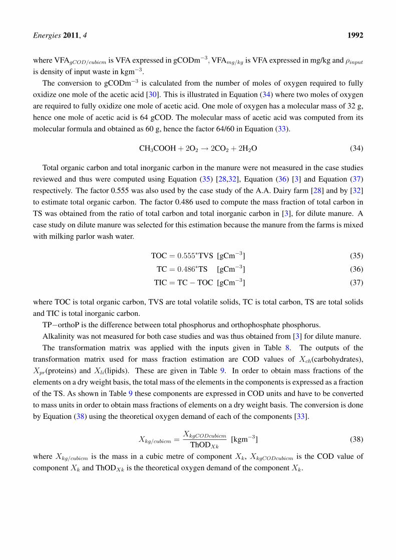
transformation matrix used for mass fraction estimation are COD values of Xch(carbohydrates),Xpr(proteins) and Xli(lipids). These are given in Table 9. In order to obtain mass fractions of theelements on a dry weight basis, the total mass of the elements in the components is expressed as a fractionof the TS. As shown in Table 9 these components are expressed in COD units and have to be convertedto mass units in order to obtain mass fractions of elements on a dry weight basis. The conversion is doneby Equation (38) using the theoretical oxygen demand of each of the components [33].

Xkg/cubicm =XkgCODcubicm

ThODXk

[kgm−3] (38)

where Xkg/cubicm is the mass in a cubic metre of component Xk, XkgCODcubicm is the COD value ofcomponent Xk and ThODXk is the theoretical oxygen demand of the component Xk.

Energies 2011, 4 1993

Table 9. Outputs of transformation matrix.

Component ThOD A.A. Dairy Noblehurst Dairyper unit mass [kgCODm−3] [kgCODm−3]

Xch 1.0627 91.695 46.657Xpr 1.5160 10.583 4.286Xli 2.8900 1.593 0.574

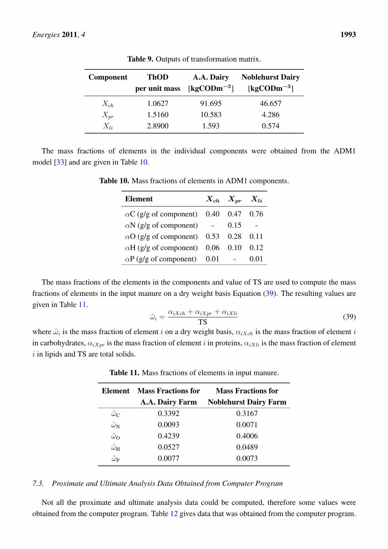
The mass fractions of elements in the individual components were obtained from the ADM1model [33] and are given in Table 10.

Table 10. Mass fractions of elements in ADM1 components.

Element Xch Xpr Xli

αC (g/g of component) 0.40 0.47 0.76αN (g/g of component) - 0.15 -αO (g/g of component) 0.53 0.28 0.11αH (g/g of component) 0.06 0.10 0.12αP (g/g of component) 0.01 - 0.01

The mass fractions of the elements in the components and value of TS are used to compute the massfractions of elements in the input manure on a dry weight basis Equation (39). The resulting values aregiven in Table 11.

ωi =αiXch + αiXpr + αiXli

TS(39)

where ωi is the mass fraction of element i on a dry weight basis, αiXch is the mass fraction of element i

in carbohydrates, αiXpr is the mass fraction of element i in proteins, αiXli is the mass fraction of elementi in lipids and TS are total solids.

Table 11. Mass fractions of elements in input manure.

Element Mass Fractions for Mass Fractions forA.A. Dairy Farm Noblehurst Dairy Farm

ωC 0.3392 0.3167ωN 0.0093 0.0071ωO 0.4239 0.4006ωH 0.0527 0.0489ωP 0.0077 0.0073

7.3. Proximate and Ultimate Analysis Data Obtained from Computer Program

Not all the proximate and ultimate analysis data could be computed, therefore some values wereobtained from the computer program. Table 12 gives data that was obtained from the computer program.

Energies 2011, 4 1994

Table 12. Proximate and ultimate analysis data from computer program’s database.

Parameter Value

S 0.001Ashes 0.150K2O 0.031Soluble VS 0.500Soluble inorganic matter 0.500Soluble P 0.500Soluble K 1.000Soluble N 0.500Density 990 kg/m3

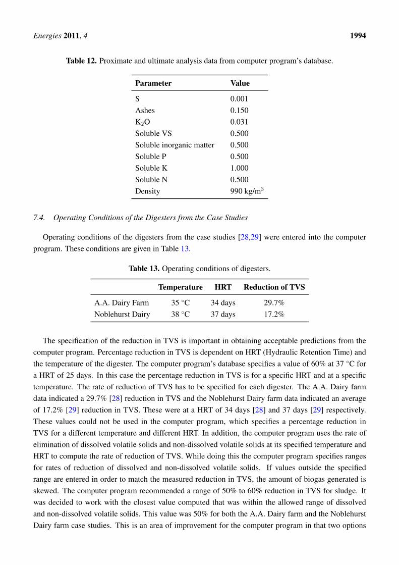
7.4. Operating Conditions of the Digesters from the Case Studies

Operating conditions of the digesters from the case studies [28,29] were entered into the computerprogram. These conditions are given in Table 13.

Table 13. Operating conditions of digesters.

Temperature HRT Reduction of TVS

A.A. Dairy Farm 35 ◦C 34 days 29.7%Noblehurst Dairy 38 ◦C 37 days 17.2%

The specification of the reduction in TVS is important in obtaining acceptable predictions from thecomputer program. Percentage reduction in TVS is dependent on HRT (Hydraulic Retention Time) andthe temperature of the digester. The computer program’s database specifies a value of 60% at 37 ◦C fora HRT of 25 days. In this case the percentage reduction in TVS is for a specific HRT and at a specifictemperature. The rate of reduction of TVS has to be specified for each digester. The A.A. Dairy farmdata indicated a 29.7% [28] reduction in TVS and the Noblehurst Dairy farm data indicated an averageof 17.2% [29] reduction in TVS. These were at a HRT of 34 days [28] and 37 days [29] respectively.These values could not be used in the computer program, which specifies a percentage reduction inTVS for a different temperature and different HRT. In addition, the computer program uses the rate ofelimination of dissolved volatile solids and non-dissolved volatile solids at its specified temperature andHRT to compute the rate of reduction of TVS. While doing this the computer program specifies rangesfor rates of reduction of dissolved and non-dissolved volatile solids. If values outside the specifiedrange are entered in order to match the measured reduction in TVS, the amount of biogas generated isskewed. The computer program recommended a range of 50% to 60% reduction in TVS for sludge. Itwas decided to work with the closest value computed that was within the allowed range of dissolvedand non-dissolved volatile solids. This value was 50% for both the A.A. Dairy farm and the NoblehurstDairy farm case studies. This is an area of improvement for the computer program in that two options

Energies 2011, 4 1995

should be provided for specification of reduction in TVS. Reduction in TVS may be obtained from thecomputer program’s database, or the program should be able to estimate biogas production based onvalues of TVS entered by users.

Dryness of the manure influent was computed using the value of TS expressed in mg/L, and massflow rate of manure Equation (40).

ωms =TSmmh

(40)

where mmh is mass flow rate of influent manure, ωms is dryness and TS is total solids.The values of mass flow rate of input waste and dryness of manure from the farms in the case studies

are given in Table 14.

Table 14. Inputs to the computer program for A.A. Dairy and Noblehurst Dairy farms.

Parameter A.A. Dairy Farm Noblehurst Dairy Farm

Dryness 0.114 0.104Manure mass flow rate 34,303.50 kg/day 67,537.80 kg/day

8. Results and Discussion

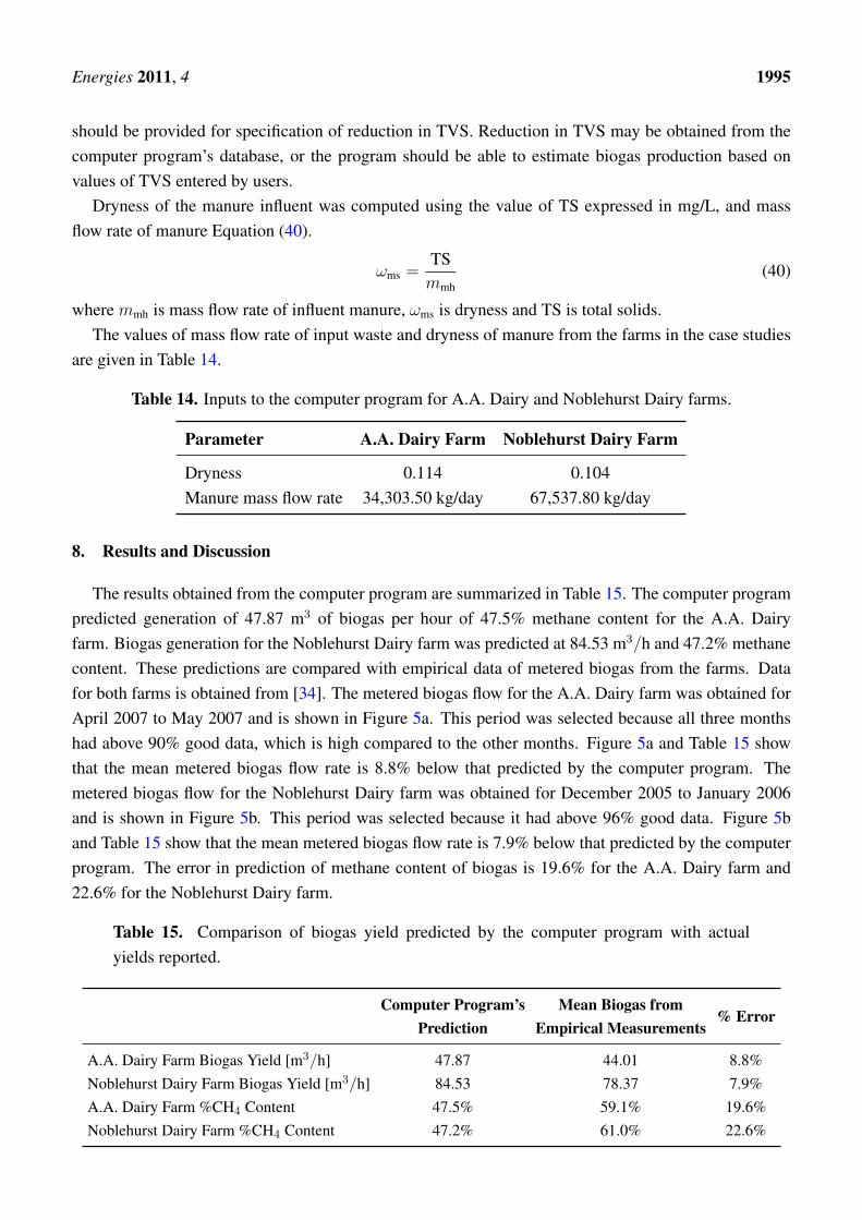
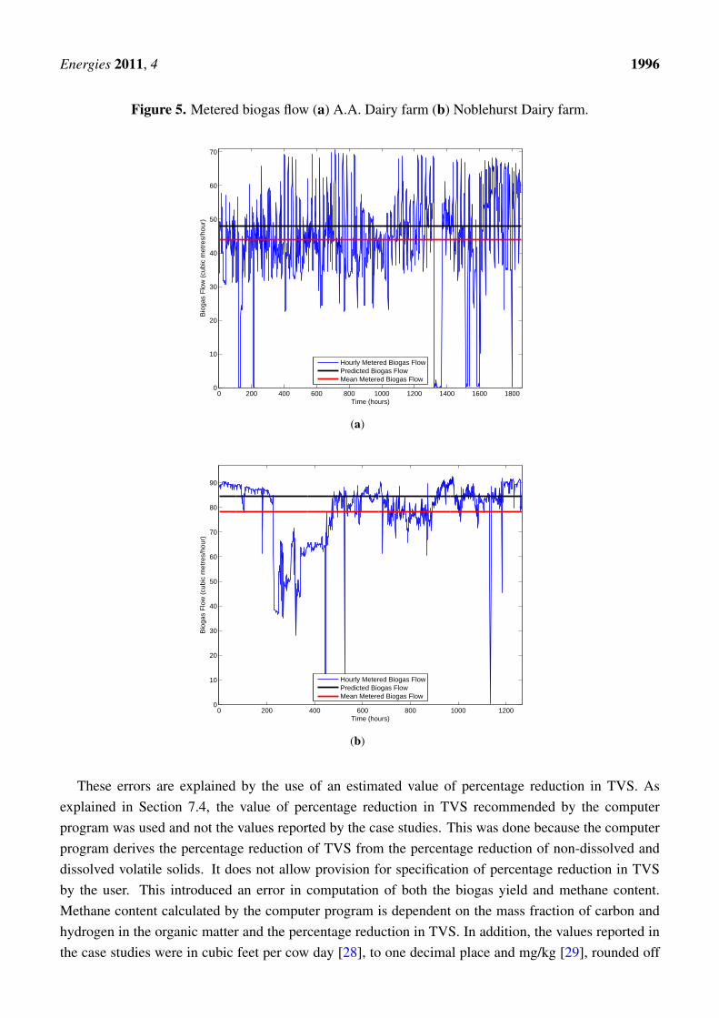
The results obtained from the computer program are summarized in Table 15. The computer programpredicted generation of 47.87 m3 of biogas per hour of 47.5% methane content for the A.A. Dairyfarm. Biogas generation for the Noblehurst Dairy farm was predicted at 84.53 m3/h and 47.2% methanecontent. These predictions are compared with empirical data of metered biogas from the farms. Datafor both farms is obtained from [34]. The metered biogas flow for the A.A. Dairy farm was obtained forApril 2007 to May 2007 and is shown in Figure 5a. This period was selected because all three monthshad above 90% good data, which is high compared to the other months. Figure 5a and Table 15 showthat the mean metered biogas flow rate is 8.8% below that predicted by the computer program. Themetered biogas flow for the Noblehurst Dairy farm was obtained for December 2005 to January 2006and is shown in Figure 5b. This period was selected because it had above 96% good data. Figure 5band Table 15 show that the mean metered biogas flow rate is 7.9% below that predicted by the computerprogram. The error in prediction of methane content of biogas is 19.6% for the A.A. Dairy farm and22.6% for the Noblehurst Dairy farm.

Table 15. Comparison of biogas yield predicted by the computer program with actualyields reported.

Computer Program’s Mean Biogas from% Error

Prediction Empirical Measurements

A.A. Dairy Farm Biogas Yield [m3/h] 47.87 44.01 8.8%Noblehurst Dairy Farm Biogas Yield [m3/h] 84.53 78.37 7.9%A.A. Dairy Farm %CH4 Content 47.5% 59.1% 19.6%Noblehurst Dairy Farm %CH4 Content 47.2% 61.0% 22.6%

Energies 2011, 4 1996

Figure 5. Metered biogas flow (a) A.A. Dairy farm (b) Noblehurst Dairy farm.

0 200 400 600 800 1000 1200 1400 1600 18000

10

20

30

40

50

60

70

Time (hours)

Bio

gas

Flo

w (

cubi

c m

etre

s/ho

ur)

Hourly Metered Biogas FlowPredicted Biogas FlowMean Metered Biogas Flow

(a)

0 200 400 600 800 1000 12000

10

20

30

40

50

60

70

80

90

Time (hours)

Bio

gas

Flo

w (

cubi

c m

etre

s/ho

ur)

Hourly Metered Biogas FlowPredicted Biogas FlowMean Metered Biogas Flow

(b)

These errors are explained by the use of an estimated value of percentage reduction in TVS. Asexplained in Section 7.4, the value of percentage reduction in TVS recommended by the computerprogram was used and not the values reported by the case studies. This was done because the computerprogram derives the percentage reduction of TVS from the percentage reduction of non-dissolved anddissolved volatile solids. It does not allow provision for specification of percentage reduction in TVSby the user. This introduced an error in computation of both the biogas yield and methane content.Methane content calculated by the computer program is dependent on the mass fraction of carbon andhydrogen in the organic matter and the percentage reduction in TVS. In addition, the values reported inthe case studies were in cubic feet per cow day [28], to one decimal place and mg/kg [29], rounded off

Energies 2011, 4 1997

to the nearest whole number. These values were converted to tonnes per hour for use in the computerprogram, which involved conversion factors given to a number of decimal places. These conversionsled to losses in accuracy, hence the additional discrepancy in actual values of biogas and methanecontent, from values predicted by the computer program. The density of manure was used to carryout these computations. This value was not reported by the case studies and was obtained from thecomputer program’s database, creating another source of error. The percentage error in methane contentpredication for the Noblehurst Dairy farm case study [29] is particularly high. This is because themeasured value includes the volume of CO2. The percentage volume of CO2 in biogas was not isolatedduring measurement [29]. Typically biogas contains 40%–75% CH4 and 25%–60% CO2 among othergases [35]. CO2 constitutes a significant volume of biogas, hence the large percentage error.

9. Conclusions

A computer program for technical and economic analysis of waste treatment processes has beendescribed with particular reference to anaerobic digestion. The computer program can be used as atool to predict the amount of biogas, electricity and heat generated from a biomass waste to energyconversion system. It also includes a module for the economic analysis of the various processes used.Two case studies have been used to predict the amount of biogas generated from anaerobic digestion ofmanure. Generation of biogas predicted by the computer program was compared with actual yields onthe farms. Ultimate analysis data was not readily available therefore a transformation matrix was usedto estimate this data. It has been shown how ultimate analysis data can be estimated given measurablemanure characteristics. Proximate analysis data was obtained from the computer program’s database.The specification of the percentage reduction in TVS has been identified as important when using thecomputer program. This is because of the method used by the computer program to obtain percentagereduction in TVS. This is key to obtaining realistic predictions of biogas generation. The percentageerrors in predicted and actual biogas yields for both case studies were within acceptable ranges. Themethane content predicted for both case studies was low. The errors in prediction of methane contentfor the case studies is attributed to estimation of reduction in percentage TVS. One of the case studiesincluded CO2 in the estimation of methane content of biogas, which increased the percentage error.

Acknowledgements

This project is part of the R&D program of the NSERC Chair entitled “Energy efficiency in electricalmachines for small renewable energy production systems” established in 2009 at Concordia University.The authors acknowledge the support of the Natural Sciences & Engineering Research Council ofCanada and Hydro-Quebec.

References

1. Batstone, D.J.; Keller, J.; Angelidaki, I.; Kalyuzhnyi, S.V.; Pavlostathis, S.G.; Rozzi, A.;Sanders, W.T.M.; Siegrist, H.; Vavilin, V.A. Anaerobic Digestion Model No. 1 (ADM1); IWAPublishing: London, UK, 2002.

Energies 2011, 4 1998

2. Page, D.I.; Hickey, K.L.; Narula, R.; Main, A.L.; Grimberg, S.J. Modeling anaerobic digestion ofdairy manure using the IWA Anaerobic Digestion Model No. 1 (ADM1). Water Sci. Technol.2008, 58, 689–695.

3. Zaher, U.; Li, R.; Jeppsson, U.; Steyer, J.; Chen, S. GISCOD: General integrated solid wasteco-digestion model. Water Res. 2009, 43, 2717–2727.

4. Jain, S.; Sharma, M.P. Power generation from MSW of haridwar city: A feasibility study. Renew.Sustain. Energy Rev. 2011, 15, 69–90.

5. Saidur, R.; Abdelaziz, E.A.; Demirbas, A.; Hossain, M.S.; Mekhilef, S. A Review on Biomass as aFuel for Boilers. Renew. Sustain. Energy Rev. 2011, 15, 2262–2289.

6. Skoulu, V.; Zabaniotou, A. Investigation of agricultural and animal wastes in Greece and theirallocation to potential application for energy production. Renew. Sustain. Energy Rev. 2007, 11,1698–1719.

7. Nizami, A.; Murphy, J.D. What type of digester configurations should be employed to producebiomethane from grass silage? Renew. Sustain. Energy Rev. 2010, 14, 1558–1568.

8. Rajeshwari, K.V.; Balakrishnan, M.; Kansal, A.; Lata, K.; Kishore, V.V.N. State-of-the-art ofanaerobic digestion technology for industrial wastewater treatment. Renew. Sustain. Energy Rev.2000, 4, 135–156.

9. Karellas, S.; Boukis, I.; Kontopoulos, G. Development of an investment decision tool for biogasproduction from agricultural waste. Renew. Sustain. Energy Rev. 2010, 14, 1273–1282.

10. Rao, P.V.; Baral, S.S.; Dey, R.; Mutnuri, S. Biogas generation potential by anaerobic digestion forsustainable energy development in India. Renew. Sustain. Energy Rev. 2010, 14, 2086–2094.

11. Jingura, R.M.; Matengaifa, R. Optimization of biogas production by anaerobic digestion forsustainable energy development in Zimbabwe. Renew. Sustain. Energy Rev. 2009, 13, 1116–1120.

12. Angelis-Dimakis, A.; Biberacher, M.; Dominguez, J.; Fiorese, G.; Gadocha, S.; Gnansounou, E.;Guariso, G.; Kartalidis, A.; Panichelli, L.; Pinedo, I.; Robba, M. Methods and tools to evaluate theavailability of renewable energy sources. Renew. Sustain. Energy Rev. 2007, 11, 1208–1226.

13. Purohit, P.; Kandpal, T.C. Techno-economics of biogas-based water pumping in India an attemptto internalize CO2 emissions mitigation and other economic benefits. Renew. Sustain. Energy Rev.2011, 15, 1182–1200.

14. Biomass Energy, Proximate and Ultimate Analyses, Woodgas. January 1998. Available online:http://www.woodgas.com/proximat.htm (accessed on 15 November 2011).

15. Bary, A.; Miles, C.; Gilbert, K. Composting of Poultry Offal Demonstration Project;Washington State University: Washington, DC, USA, 2005. Available online:http://agsyst.wsu.edu/PoultryOffal.pdf (accessed on 15 November 2011).

16. Agriculture, Food and Rural Development (AFRD). Manure Composting Manual; AFRD:Edmonton, Canada, 2006. Available online: http://www1.agric.gov.ab.ca/$department/deptdocs.nsf/all/agdex8875 (accessed on 15 November 2011).

17. Arrouge, T. Le compostage des Boues de Papetieres. Aspects de la Problematique Pour le Quebec.Master Thesis, Universite de Sherbrooke, Sherbrooke, Canada, 1997.

18. Rosenow, P.; Tiry, M.J. Composting Dairy Manure for the Commercial Markets. In Proceedings ofthe Manure Management Conference, Ames, IA, USA, 10–12 February 1998.

Energies 2011, 4 1999

19. Browne, M.J.; Whipps, A.P. Development of the sludge thermal drying option for south west water.J. Chart. Inst. Water Environ. Manag. 1995, 9, 445–453.

20. Pommier, S.; Llamas, A.M.; Lefebvre, X. Analysis of the Outcome of Shredding Pre-treatment onthe Anaerobic Biodegradability of Paper and Cardboard Materials. Bioresour. Technol. 2010, 101,463–468.

21. Moletta, R. La Methanisation; Lavoisier: Paris, France, 2008.22. Vor Environnement, Traitement anaerobie, fiche technique Methavor, 2005. Available online:

http://methavor.vor.fr (accessed on 15 November 2011).23. Buchanan, J.R.; Seabloom, R.W. Aerobic Treatment of Wastewater and Aerobic Treatment Units.

Module Text, University Curriculum Development for Decentralized Wastewater Management.November 2004. Available online: http://www.onsiteconsortium.org/files/Aaerobic_Treatment_&_ATUs.pdf (accessed on 15 November 2011).

24. Samson, R.; Guiot, S. Les Nouveaux Secteurs a Fort Potentiel de Developpement en DigestionAnaerobie; Centre Quebecois de Valorisation de la Biomasse: Quebec, Canada, 1990.

25. The Energy Conservation Center, Japan. Japan Energy Conservation Handbook 2005/2006.Available online: http://www.asiaeec-col.eccj.or.jp/databook/2005-2006e/index.html (accessed on15 November 2011).

26. Goldstein, L.; Hedman, B.; Knowles, D.; Freedman, S.I.; Woods, R.; Schweizer, T. Gas-FiredDistributed Energy Resource Technology Characterization, Publication of National RenewableEnergy Laboratory for the United States Department of Energy. October 2003. Available online:http://www.eea-inc.com/dgchp reports/TechCharNREL.pdf (accessed on 15 November 2011).

27. Szonyi, A.J.; Fenton, R.G.; White, J.A.; Agee, M.H.; Case, K.E. Principles of EngineeringEconomic Analysis, Canadian ed.; John Wiley and Sons: Toronto, Canada, 1982.

28. Martin, J.H. A Comparison of Dairy Cattle Manure Management With and without AnaerobicDigestion and Biogas Utilization; Eastern Research Group, Inc.: Lexington, MA, USA, 2004.

29. Gooch, C.A.; Inglis, S.F.; Wright, P.E. Biogas Distributed Generation Systems Evaluation andTechnology Transfer; NYSERDA Project No. 6597, Interim Report for May 2001 to May 2005.New York State Energy Research and Development Authority: New York, NY, USA, 2007.

30. Zaher, U.; Buffiere, P.; Steyer, J.P.; Chen, S. A procedure to estimate proximate analysis of mixedorganic wastes. Water Environ. Res. 2009, 81, 407–415.

31. Gooch, C.; Pronto, J. Anaerobic Digestion at A.A. Dairy, Case Study, February 2008. Availableonline: http://www.manuremanagement.cornell.edu/Pages/General_Docs/Case_Studies/AA_Case_Study.pdf (accessed on 17 November 2011).

32. Martin, J.H. An Evaluation of A Mesophilic, Modified Plug Flow Anaerobic Digester for DairyCattle Manure, July 2005. Available online: http://www.ghdinc.net/gordondale_report_final.pdf(accessed on 17 November 2011).

33. de Gracia, M.; Sancho, L.; Garcia-Heras, J.L.; Vanrolleghem, P.; Ayesa, E. Mass and chargeconservation check in dynamic models: Application to the new ADM1 model. Water Sci. Technol.2006, 53, 225–240.

34. NYSERDA DG/CHP Integrated Data System. Available online: http://chp.nyserda.org/facilities/index.cfm (accessed on 30 October 2011).

Energies 2011, 4 2000

35. Bilitewski, B.; Hardtle, G.; Marek, K.; Weissbach, A.; Boeddicker, H. Waste Management;Springer: Berlin, Germany, 1997.

Nomenclature

ADM1 Anaerobic Digester Model No. 1C CarbonC/N carbon-to-nitrogenCH4 methaneCHP Combined Heat and PowerCl ChlorineCO2 Carbon dioxideCOD Chemical Oxygen DemandCODp particulate Chemical Oxygen DemandCODs soluble Chemical Oxygen DemandFS Fixed SolidsH HydrogenHRT Hydraulic Retention TimeH2O waterH2S Hydrogen SulphideHCV Higher Calorific ValueIRR Internal Rate of ReturnIWA International Water AssociationK PotassiumK2O Potassium oxideLCV Lower Calorific Valuemh wet massmol molems dry massMI inorganic matterMSW Municipal Solid WasteN NitrogenNH3 ammoniaNPV Net Present ValueO OxygenorthoP ortho-PhosphorusP PhosphorusP2O5 Phosphorus pentoxideS SulphurScat Alkalinitytmh tonnes of wet masstms tonnes of dry mass

Energies 2011, 4 2001

TAN Total Ammonia NitrogenTC Total CarbonTIC Total Inorganic CarbonTKN Total Kjeldahl NitrogenTS Total SolidsTVA Total Volatile AcidsTVS Total Volatile SolidsVFA Volatile Fatty AcidsVS Volatile Solids

c⃝ 2011 by the authors; licensee MDPI, Basel, Switzerland. This article is an open access articledistributed under the terms and conditions of the Creative Commons Attribution license(http://creativecommons.org/licenses/by/3.0/).