Energetic outer zone electron loss timescales

during low geomagnetic activity

Nigel P. Meredith,1 Richard B. Horne,1 Sarah A. Glauert,1 Richard M. Thorne,2

Danny Summers,3,4 Jay M. Albert,5 and Roger R. Anderson6

Received 3 November 2005; revised 1 February 2006; accepted 9 February 2006; published 27 May 2006.

[1] Following enhanced magnetic activity the fluxes of energetic electrons in the Earth’souter radiation belt gradually decay to quiet-time levels. We use CRRES observations toestimate the energetic electron loss timescales and to identify the principal lossmechanisms. Gradual loss of energetic electrons in the region 3.0 � L � 5.0 occurs duringquiet periods (Kp < 3�) following enhanced magnetic activity on timescales ranging from1.5 to 3.5 days for 214 keV electrons to 5.5 to 6.5 days for 1.09 MeV electrons. Theintervals of decay are associated with large average values of the ratio fpe/fce (>7),indicating that the decay takes place in the plasmasphere. We compute loss timescales forpitch-angle scattering by plasmaspheric hiss using the PADIE code with wave propertiesbased on CRRES observations. The resulting timescales suggest that pitch angle scatteringby plasmaspheric hiss propagating at small or intermediate wave normal angles isresponsible for electron loss over a wide range of energies and L shells. The regionwhere hiss dominates loss is energy-dependent, ranging from 3.5 � L � 5.0 at 214 keV to3.0 � L � 4.0 at 1.09 MeV. Plasmaspheric hiss at large wave normal angles does notcontribute significantly to the loss rates. At E = 1.09 MeV the loss timescales areoverestimated by a factor of �5 for 4.5 � L � 5.0. We suggest that resonant wave-particleinteractions with EMIC waves, which become important at MeV energies for largerL (L > �4.5), may play a significant role in this region.

Citation: Meredith, N. P., R. B. Horne, S. A. Glauert, R. M. Thorne, D. Summers, J. M. Albert, and R. R. Anderson (2006), Energetic

outer zone electron loss timescales during low geomagnetic activity, J. Geophys. Res., 111, A05212, doi:10.1029/2005JA011516.

1. Introduction

[2] Energetic electrons (E > 100 keV) in the Earth’sradiation belts are generally confined to two distinctregions. The inner radiation belt lies in the range 1.2 < L< 2.5 and exhibits long-term stability. In contrast, the outerradiation belt, which lies in the range 3 < L < 7, is highlydynamic, particularly during enhanced magnetic activity[e.g., Paulikas and Blake, 1979; Baker et al., 1986, 1994,1997; Li et al., 1997; Reeves et al., 1998]. This variability iscaused by an imbalance between acceleration and lossprocesses both of which tend to be enhanced duringmagnetically disturbed periods [e.g., Summers et al.,

2004]. Understanding this variability is important sinceenhanced fluxes of relativistic electrons (E > 1 MeV)damage satellites in Earth orbit and pose a risk to humansin space. Indeed, enhanced fluxes of relativistic electronshave been associated with a number of spacecraft anomaliesand even failures [Baker et al., 1998a; Baker, 2001].Consequently, predicting their appearance has become oneof the outstanding challenges of magnetospheric physics.Furthermore, energetic electrons can penetrate to low alti-tudes where they affect the ionization, conductivity, andchemistry of the stratosphere and mesosphere [e.g., Thorne,1980; Lastovicka, 1996; Callis et al., 1998], thereby pro-viding an important coupling mechanism between themagnetosphere and the middle atmosphere.[3] Electrons with energies up to a few hundred keV are

injected into the inner magnetosphere during storms andsubstorms. Injection of electrons in the energy range 10–100 keV into the outer zone leads to the excitation of intensewhistler mode chorus waves outside the plasmasphere onthe dawnside of the magnetosphere [e.g., Tsurutani andSmith, 1977; Meredith et al., 2001, 2003a]. At higherenergies, injected electrons with energies in the range100–300 keV form a seed population of electrons [e.g.,Baker et al., 1998b; Obara et al., 2000] which maysubsequently be accelerated to relativistic energies by pro-cesses acting within the magnetosphere itself [Li et al.,1997]. While several acceleration mechanisms have been

JOURNAL OF GEOPHYSICAL RESEARCH, VOL. 111, A05212, doi:10.1029/2005JA011516, 2006

1British Antarctic Survey, Natural Environment Research Council,Cambridge, UK.

2Department of Atmospheric and Oceanic Sciences, University ofCalifornia, Los Angeles, Los Angeles, California, USA.

3Department of Mathematics and Statistics, Memorial University ofNewfoundland, St John’s, Newfoundland, Canada.

4Also at School of Physics, University of KwaZulu-Natal, Durban,South Africa.

5Space Vehicles Directorate, Air Force Research Laboratory, HanscomAir Force Base, Massachusetts, USA.

6Department of Physics and Astronomy, University of Iowa, Iowa City,Iowa, USA.

Copyright 2006 by the American Geophysical Union.0148-0227/06/2005JA011516

A05212 1 of 13

proposed (see the reviews by Li and Temerin [2001], Horne[2002], and Friedel et al. [2002]), recent experimental andmodelling work suggests that the acceleration is caused by acombination of enhanced inward radial diffusion driven byULF waves [e.g., Elkington et al., 1999; Liu et al., 1999;Hudson et al., 2000] and local, chorus-driven accelerationoutside the plasmapause [e.g., O’Brien et al., 2003; Horneet al., 2006; Summers et al., 2005; Varotsou et al., 2005].However, during quiet conditions following enhanced mag-netic activity, the acceleration processes are ineffective andthe energetic electrons gradually decay to their quiet timevalues. In order to understand radiation belt variability anddevelop more realistic physical models, it is essential tounderstand and quantify the decay processes. The periods ofgradual decay provide a unique possibility to isolate the lossprocesses acting during these intervals and to determine thedecay lifetimes.[4] There are several loss mechanisms that operate during

quiet time decay. Coulomb collisions with atmosphericconstituents are important in the inner zone and are thedominant loss mechanism closest to the Earth, while reso-nant interactions with plasma waves become increasinglyimportant farther out. The region where Coulomb collisionsdominate is energy-dependent, ranging from L < 2.2 for100 keV electrons to L < 1.4 for 1.5 MeV electrons [Abeland Thorne, 1998]. Ground-based VLF transmitters, usedfor communications with submarines, leak out of theatmosphere at night and propagate in the inner magneto-sphere in the whistler mode. These waves are mostimportant just outside the region dominated by Coulombcollisions. Using average wave characteristics as input totheir model, Abel and Thorne [1998] showed that pitch-angle scattering by VLF transmitters is likely to be the mosteffective loss mechanism for 100 keV electrons in theregion from 2.2 < L < 2.8 and for 1.5 MeV electrons inthe region 1.4 < L < 2.2. Lightning-generated whistlers aremost effective just outside the region dominated by VLFtransmitters, being most effective from 2.8 < L < 4.4 for 100keV electrons and from 2.2 < L < 2.6 for 1.5 MeV electrons[Abel and Thorne, 1998]. Farther out, but remaining insidethe plasmapause, resonant interactions with both plasma-spheric hiss and electromagnetic ion cyclotron (EMIC)waves are believed to dominate [Thorne et al., 1973; Lyonset al., 1972; Albert, 1994; Summers and Thorne, 2003;Summers, 2005]. Outside of the plasmapause, whistlermode chorus waves can contribute effectively to the lossof energetic electrons [Horne and Thorne, 2003; O’Brien etal., 2004; Thorne et al., 2005a; Summers et al., 2005].[5] The studies described above have identified loss

timescales in various regions but have been limited in thecoverage of energies and L shells. Here we provide a moreextensive survey using the CRRES data set. The objectivesare to determine experimentally the loss timescales forenergetic electrons over a wide range of energies and Lshells, to determine the conditions associated with loss, andto identify the principal loss mechanisms.

2. Instrumentation

[6] The Combined Release and Radiation Effects Satellite(CRRES) is particularly well-suited to studies of wave-particle interactions in the radiation belts both because of

its orbit and sophisticated suite of wave and particle instru-ments [Johnson and Kierein, 1992]. The spacecraft waslaunched on 25 July 1990 and operated in a highly ellipticalgeosynchronous transfer orbit with a perigee of 305 km, anapogee of 35,768 km, and an inclination of 18�. The orbitalperiod was approximately 10 hours, and the initial apogeewas at a magnetic local time (MLT) of 0800 MLT. Themagnetic local time of apogee decreased at a rate ofapproximately 1.3 hours per month until the satellite failedon 11October 1991, when its apogee was at about 1400MLT.The satellite swept through the heart of the radiation belts onaverage approximately 5 times per day, providing goodcoverage of this important region for almost 15 months.[7] The electron data used in this study were collected by

the Medium Electrons A (MEA) experiment. This instru-ment, which used momentum analysis in a solenoidal field,had 17 energy channels ranging from 153 keV to 1.58 MeV[Vampola et al., 1992]. The wave data used in this studywere provided by the Plasma Wave Experiment. Thisexperiment provided measurements of electric fields from5.6 Hz to 400 kHz, using a 100 m tip-to-tip long wireantenna, with a dynamic range covering a factor of at least105 in amplitude [Anderson et al., 1992]. The electric fielddetector was thus able to detect waves from below the lowerhybrid resonance frequency (fLHR) to well above the upperhybrid resonance frequency (fUHR) for a large fraction ofeach orbit.

3. Data Analysis

3.1. CRRES Database

[8] In order to study electron loss rates and the role ofplasmaspheric hiss in the loss process, we constructed adatabase from the wave and particle data. The electrondifferential number flux perpendicular to the ambient mag-netic field for each energy level of the MEA instrument andthe ratio fpe/fce, together with the magnetic field intensitiesin the range 0.1 � f � 2 kHz and the electric field intensitiesin the range fce < f < 2fce were rebinned as a function of halforbit (outbound and inbound) and L in steps of 0.1 L asdetailed by Meredith et al. [2004]. The data were recordedtogether with the universal time (UT), magnetic latitude(lm), magnetic local time (MLT), and time spent in each binwith the same resolution. The subsequent analysis of theparticle data was restricted to the equatorial perpendicularfluxes, defined to be observations within ±15� of themagnetic equator to reduce latitudinal effects in measure-ments of the perpendicular flux and the ratio fpe/fce. If weassume a dipole field then this criterion restricts the analysisto equatorial pitch angles, aeq, in the range (60� � aeq �120�).

3.2. Determination of the Loss Timescale

[9] During quiet periods the energetic electron flux, J,often exhibits an exponential decay. To quantify the decayand compare results for different energies and L shells, wehave calculated a loss timescale, t, by fitting an exponentialfunction of the form J = Ae�(t/t) to periods of gradual decay.To prevent the fits from being dominated by the mostintense fluxes, we obtain the decay time constant by fittinga linear function to the natural logarithm of the flux. Thefitting intervals are selected automatically to prevent ob-

A05212 MEREDITH ET AL.: ENERGETIC ELECTRON LOSS TIMESCALES

2 of 13

A05212

server bias from influencing the results. We measure thestrength of the linear relationship between the naturallogarithm of the flux and the decay time using the Pearsoncorrelation coefficient. The value of this coefficient variesfrom �1 to +1 with �1 indicating a perfect negative(inverse) correlation, 0 no correlation, and +1 a perfectpositive correlation. We proceed as follows. The Pearsoncorrelation coefficient is determined for the first ten points.If the Pearson coefficient is negative with an absolute valueless than 0.95 or positive the fit is discarded and the startingpoint is incremented by one point. The process is thenrepeated throughout the data set. When the Pearson corre-lation coefficient is negative with an absolute value greaterthan 0.95 the number of points included in the fit isincreased in unit increments up to a maximum of 75 points.The fitting interval is then chosen to be the fit with thelargest absolute value of the Pearson coefficient. The wholeprocess is then repeated starting from the next point after thefitting interval. The process is repeated for the whole dataset as a function of time for selected energies and L shells.[10] We tested the sensitivity of the technique to the

minimum number of points in the fit by using a minimumof five points as compared with ten and found that theresults were relatively insensitive to the minimum numberof point in the fit. The nature of the fitting technique is suchthat we do not fit to intervals with less than five pointswhich corresponds to a minimum duration of approximately25 hours due to the orbital period of CRRES. Periods of fastdecay, associated with the main phase of geomagneticstorms, are thus excluded from the fits and we concentrateon the periods of more gradual decay following enhancedmagnetic activity.

3.3. Determination of the Plasma Environment

[11] The ratio of the electron plasma frequency, fpe, to theelectron gyrofrequency, fce, is an important parameter forelectron acceleration and loss in the inner magnetosphere[Summers et al., 1998; Horne, 2002]. Given the presence ofthe appropriate whistler mode waves, low values of thisratio are associated with the plasma trough and energy andpitch-angle diffusion [Summers et al., 1998; Horne et al.,2003]. High values of this ratio are associated with theplasmasphere, pitch-angle scattering and subsequent loss tothe atmosphere [Lyons et al., 1972; Summers et al., 1998;Summers, 2005].[12] Loss processes inside the plasmapause may be very

different to those outside and have different relative impor-tance. It is therefore helpful to identify the location of theobservations with respect to the plasmapause, which can beinferred from measurements of the ratio of fpe/fce. In order toconstruct their empirical plasmaspheric density model,Sheeley et al. [2001] adopted an L-shell dependent bound-ary number density, given by nb = 107(6.6/L)4 m�3, toseparate plasmaspheric-like and trough-like values. Densi-ties below nb were considered trough-like and densitiesabove nb were considered to be plasmaspheric-like. We usethe same criterion and express the boundary ratio (fpe/fce)b interms of the boundary number density, nb, and the localmagnetic field strength, B, as

fpe=fce� �

b¼

ffiffiffiffiffiffiffiffiffiffiffiffiffiffiffiffiffiffiffiffiffiffiffiffiffinbme=�0B2ð Þ

pð1Þ

If we assume a dipole field, then

B ¼ Beq

ffiffiffiffiffiffiffiffiffiffiffiffiffiffiffiffiffiffiffiffiffiffiffiffiffiffiffi1þ 3 cos2 qð Þ

p=L3 sin6 q ð2Þ

where Beq is the mean value of the magnetic field on theequator at the surface of the Earth, and q is the colatitude.Substituting in values for the appropriate constants, andkeeping the plasma density constant with magnetic latitude,we obtain

fpe=fce� �

b¼ 1:416L sin6 q=

ffiffiffiffiffiffiffiffiffiffiffiffiffiffiffiffiffiffiffiffiffiffiffiffiffiffiffi1þ 3 cos2 qð Þ

pð3Þ

The boundary value, separating the plasmasphere-likevalues from trough-like values, for measurements madewithin 15� of the magnetic equator on a given geomagneticfield line thus lies in the range 1.23L ± 0.18L. Typically, inthe plasmasphere, the ratio fpe/fce is much larger than theboundary value, and, in the plasma trough, the ratio fpe/fce ismuch smaller than the boundary value.

4. Results

4.1. L = 3.55

[13] The Kp index and the equatorial perpendicular dif-ferential number flux of 1.09 MeV electrons at L = 3.55 areplotted as a function of day number from 01/01/90 for theentire CRRES mission in Figure 1. The Kp index has beensmoothed using a 15 hour running mean and the electrondata have been color-coded according to the value of theratio fpe/fce. In the equatorial region at L = 3.55, (fpe/fce)b =4.4 ± 0.6 so that measurements made when fpe/fce is aboveor below �4.4 may be regarded as plasmaphere-like ortrough-like, respectively.[14] Large increases in the flux of relativistic electrons are

associated with increased magnetic activity as monitored bythe Kp index, and, in particular, when Kp > 5. These eventsare associated with magnetic storms, as monitored by theDst index. The increase can be very rapid, such as the eventon day number 332, or may take place over a timescale ofdays. The very rapid events may be attributed to eithershock acceleration [Li et al., 1993; Hudson et al., 1997] orthe inward movement of the inner edge of the outer belt.The longer-lasting flux increases take place over a period of2–4 days and are associated with low values of fpe/fce andhence the trough region. These events are known to beassociated with enhanced levels of magnetic activity, en-hanced chorus activity, and enhanced fluxes of seed elec-trons [e.g., Meredith et al., 2002a, 2002b, 2003b; Miyoshi etal., 2003].[15] In the absence of further significant magnetic activity

(Kp < �3) the elevated poststorm relativistic electron fluxesgradually decay to quiet time values. During quiet periodsthe fluxes may fall by as much as two orders of magnitudeover a period of �20 days. The best fits to the selecteddecay periods are overplotted on the data and yield a decaytime constant of 5.7 ± 0.6 days, where the quoted error, hereand henceforth, is the error of the mean. These periods ofgradual decay are all associated with elevated values of theratio fpe/fce. The average value of fpe/fce for the fittingintervals is 9.5 ± 0.2, indicating that these periods of gradualflux decay take place largely in the plasmasphere. The

A05212 MEREDITH ET AL.: ENERGETIC ELECTRON LOSS TIMESCALES

3 of 13

A05212

average value of the Kp index during the intervals of decayis 2.23 ± 0.02, indicative of relatively quiet magneticactivity.

4.2. L = 4.55

[16] The Kp index and the equatorial perpendicular differ-ential number flux of 1.09 MeV electrons at L = 4.55are plotted as a function of day number from 01/01/90 inFigure 2. In the equatorial region at L = 4.55 measurementsmade when fpe/fce is above or below�5.6 may be regarded asplasmaphere-like or trough-like, respectively. At L = 4.55 wesee a larger number of flux enhancements due to the fact thatweaker storms can result in flux increases at larger L. Theincreases are again associated with low values of fpe/fce,typically fpe/fce < 4. At L = 4.55 the decay time-constant is5.3 ± 0.6 days, comparable to the timescale at L = 3.55. Theaverage value of fpe/fce during the decay periods is 11.0 ± 0.4,consistent with electron decay in this region taking place inthe plasmasphere. The average value of the Kp index duringthe intervals of decay is 1.83 ± 0.02, indicative of relativelyquiet magnetic activity.[17] The Kp index and the equatorial perpendicular elec-

tron differential number flux of 214 keV electrons at L =4.55 are shown for comparison with the MeV electrons inFigure 3. During high magnetic activity the ratio fpe/fce islow denoting the plasma trough. The flux levels alsotend remain high. The loss timescales are more rapid thanat 1.09 MeV, and, during quiet periods, the fluxes may fallby as much as two orders of magnitude over a period of�6 days. The best fits to the selected decay periods yield adecay time constant of 2.0 ± 0.1 days, a factor of 2.65 times

faster than at 1.09 MeV. The average value of the ratio fpe/fcefor the fitting intervals is 9.9 ± 0.3, consistent with electrondecay at this energy also occurring in the plasmasphere. Theintervals of decay again occur during quiet magnetic con-ditions when the average value of the Kp index is 1.7 ± 0.1.

4.3. 3 ����� L ����� 5

[18] The analysis was repeated for different energies andL shells and the resulting decay timescales are plotted as afunction of energy and L shell for the region 3 � L � 5 inFigure 4. At 1.09 MeV the decay timescales lie in the range5.5–6.5 days and show little variation with L shell. Incontrast, at 510 keV the decay timescales are less, rangingfrom 2.5 to 5.5 days, and display a general tendency toincrease with increasing L for L > 3.6. The shortest time-scales are seen at 214 keV, ranging from 1.5 to 3.5 days, anddisplay a tendency to increase with increasing L for L > 4.Beyond L = �5 the data exhibit more variability and it is notpossible to calculate reliable average loss timescales usingour fitting criteria. The fitting technique also breaks downinside L = 3.3 for 214 keVelectrons, due to increased scatterbetween neighboring data points.[19] The average value of the ratio fpe/fce during the

selected intervals of gradual decay for 214 keV, 510 keV,and 1.09 MeV electrons at each L shell studied is shown inFigure 5. The dashed line represents the boundary valuebetween the trough and plasmaspheric-like material withtrough-like material below the line and plasmaspheric-likematerial above the line. Here fpe/fce lies well above the linefor all energies and L shells suggesting that the intervals ofgradual decay take place in the plasmasphere.

Figure 1. The Kp index and the equatorial perpendicular differential number flux of 1.09 MeVelectronsat L = 3.55 as a function of day number for the entire CRRES mission. The Kp index has been smoothedusing a 15-hour running mean and the data points are color-coded according to the value of fpe/fce at thetime of the measurement. The Kp value of 3� is represented by the horizontal dashed line. The best fits tothe selected decay periods are overplotted on the data.

A05212 MEREDITH ET AL.: ENERGETIC ELECTRON LOSS TIMESCALES

4 of 13

A05212

[20] The average value of the Kp index during theselected intervals of gradual decay for 214 keV, 510 keV,and 1.09 MeV electrons at each L shell studied is shown inFigure 6. The intervals of decay are associated with lowvalues of Kp (Kp � 3�), indicative of quiet time conditions.There is also a tendency for the average value of Kp during

the decay periods to decrease with increasing L shell. Sincethe quiet-time decay takes place largely in the plasma-sphere, quiet-time decay only becomes possible at a givenlocation once the plasmapause has expanded beyond thelocation, which can only occur when Kp becomes small[Carpenter and Anderson, 1992]. On average, quieter

Figure 3. The Kp index and the equatorial perpendicular differential number flux of 214 keV electronsat L = 4.55 in the same format as Figure 1.

Figure 2. The Kp index and the equatorial perpendicular differential number flux of 1.09 MeVelectronsat L = 4.55 in the same format as Figure 1.

A05212 MEREDITH ET AL.: ENERGETIC ELECTRON LOSS TIMESCALES

5 of 13

A05212

Figure 4. Measured electron loss timescales versus L shell for 214 keV, 510 keV, and 1.09 MeVelectrons.

Figure 5. The average value of fpe/fce during the selected intervals of decay versus L shell for 214 keV,510 keV, and 1.09 MeV electrons. The dashed line represents the boundary value between trough andplasmaspheric-like material.

A05212 MEREDITH ET AL.: ENERGETIC ELECTRON LOSS TIMESCALES

6 of 13

A05212

magnetic conditions and smaller values of Kp are requiredwith increasing L which explains the observed trend.

5. Loss Mechanisms

[21] The observations of gradual periods of electron losslasting for several days or more are largely associated withhigh values of fpe/fce and hence take place in the plasma-sphere. While observations on the duskside cannot confirmthat the electrons spend all of their drift orbits inside theplasmapause, the observations of loss associated with largevalues of fpe/fce on the dawnside suggest that during theperiods of gradual decay, the electrons do indeed remaininside the plasmapause for the majority of their drift orbits.[22] The chorus waves, thought to play a role in the

acceleration of electrons to relativistic energies in the outerradiation belt, tend to be confined to the low-density regionsoutside of the plasmapause and so are unlikely to play a rolein electron loss in the plasmasphere. On the other hand,electromagnetic ion cyclotron (EMIC) waves, plasma-spheric hiss, lightning-generated whistlers, and VLF trans-mitter signals are observed in the plasmasphere and may allcontribute to pitch-angle scattering and subsequent electronloss in this region [e.g., Albert, 2003; Summers and Thorne,2003; Thorne et al., 2005b; Summers, 2005].[23] Electromagnetic ion cyclotron waves, which propa-

gate in bands below the proton gyrofrequency, are able tointeract with energetic electrons resulting in pitch-anglescattering and loss to the atmosphere [e.g., Summers andThorne, 2003; Albert, 2003]. However, electron minimumresonant energies are only observed to fall below 2 MeV inthe region L > 4.5 when fpe/fce > 10 and largely occur on the

duskside [Meredith et al., 2003c]. Furthermore, these lower-energy scattering events tend to be associated with magneticstorms. It is therefore unlikely that EMIC waves will playthe most significant role in the loss of electrons withenergies in the range 100 keV < E < 1 MeV during therelatively quiet periods associated with gradual electrondecay and, in particular, inside of L = 4.5.[24] Plasmaspheric hiss is a broadband, structureless

emission which occurs in the frequency range from100 Hz to several kHz. This whistler mode emission isobserved inside of the plasmapause and is most intenseduring storms, although the emissions also persist duringrelatively quiet times [e.g., Smith et al., 1974; Thorne et al.,1977; Meredith et al., 2004]. The minimum resonantenergies for a band of hiss in the range 3.0 � L � 5.0 aretypically less than 100 keV, and thus the waves can resonatewith electrons with E � 100 keV. Plasmaspheric hiss couldthus play an important role in electron loss inside theplasmapause and, in particular, to the gradual loss observedwhen quiet periods follow geomagnetic storms.

6. Estimation of Loss Rates Due toPlasmaspheric Hiss

[25] We investigate the role of plasmaspheric hiss as aloss process using wave observations from the CRRESspacecraft to calculate pitch-angle diffusion rates for elec-trons. The diffusion rates are calculated using the PADIE(Pitch Angle and Energy Diffusion of Ions and Electrons)code [Glauert and Horne, 2005].[26] Since resonant scattering by hiss is not sensitive to

the ion composition, an electron/proton plasma is assumed.

Figure 6. The average value of the Kp index during the selected intervals of decay versus L shell for214 keV, 510 keV, and 1.09 MeV electrons.

A05212 MEREDITH ET AL.: ENERGETIC ELECTRON LOSS TIMESCALES

7 of 13

A05212

The determination of the diffusion coefficients then requiresknowledge of the distribution of the wave power spectraldensity with frequency and wave normal angle, togetherwith the ratio fpe/fce, wave mode, and the number ofresonances. We calculate the bounce-averaged pitch-anglediffusion coefficients for whistler mode hiss for Landau(n = 0) and ±5 cyclotron harmonic resonances.[27] The waves are assumed to have a Gaussian frequency

distribution given by

B2 wð Þ ¼ A2 exp � w� wm

dw

� �2� �wlc � w � wuc

0 otherwise;

8<: ð4Þ

where B2 is the power spectral density of wave magneticfield (in T2 Hz�1), wm and dw are the frequency ofmaximum wave power and bandwidth, respectively, wlc andwuc are lower and upper bounds to the wave spectrumoutside which the wave power is zero, and A2 is anormalization constant given by

A2 ¼ jBwj2

dw2ffiffiffip

p erfwm � wlc

dw

� �þ erf

wuc � wm

dw

� �h i�1

ð5Þ

where Bw is the wave amplitude in units of Tesla. Thedistribution of wave normal angles y is also assumed to beGaussian, given by

g Xð Þ ¼ exp � X � Xm

dX

� �2 !

Xlc � X � Xuc

0 otherwise;

8><>: ð6Þ

where X = tan(y), dX is the angular width, Xm is the peak,and Xlc and Xuc are the lower and upper bounds to the wavenormal distribution outside of which the wave power iszero.[28] Once the pitch-angle diffusion rate is calculated, the

timescale for the electrons to pitch-angle scatter into the losscone can be determined. Following previous work [Lyons etal., 1972; Albert, 1994], we assume that the electrondistribution function, f, satisfies the one-dimensionalpitch-angle diffusion equation,

@f

@t¼ 1

T sin 2a0

@

@a0

hDaaiT sin 2a0

@f

@a0

� �� �ð7Þ

where a0 is the equatorial pitch-angle, hDaa(a0)i is thebounce-averaged pitch-angle diffusion coefficient in unitsof s�1, and

T a0ð Þ ¼ 1:30� 0:56 sina0 ð8Þ

is an approximation to the mirror latitude dependence of thebounce period.[29] By assuming that f can be factorized into time-

dependent and pitch-angle dependent functions,

f a0; tð Þ ¼ F tð Þg a0ð Þ; ð9Þ

and that the precipitation lifetime, t is given by

t ¼ �F

dF=dt; ð10Þ

equation (7) becomes

@

@a0

hDaaiT sin 2a0

dg

da0

� �þ T sin 2a0

tg ¼ 0: ð11Þ

Equation (11), together with the boundary conditions

g aLð Þ ¼ 0; ð12Þ

dg

da0

p2

� �¼ 0; ð13Þ

2

Z p2

aL

g sina0da0 ¼ 1; ð14Þ

where aL is the loss cone pitch-angle, can be cast as a two-point boundary value problem in four variables [Albert,1994], which can be solved to obtain the lifetime, t. Wesolved this boundary value problem with a routine from theNAG library, D02GAF, which uses a finite differencemethod combined with a deferred correction technique anda Newton iteration.

6.1. Wave Model

[30] We use a model based on CRRES observations forthe plasmaspheric hiss wave intensities. Since whistlermode chorus waves can fall into the hiss band outside ofL � 3.5, we adopt a criterion based on the wave amplitudein the ECH band (fce < f < 2fce) to distinguish betweenplasmaspheric hiss and chorus. Specifically, we use thecriterion that the ECH wave amplitude for frequencies inthe range fce < f < 2fce must be less than 0.0005 mV m�1 inorder for wave emissions below fce in the frequency range0.1 � f � 2 kHz to be identified as plasmaspheric hiss[Meredith et al., 2004].[31] Energetic electrons (E > 200 keV) in the Earth’s

outer radiation belt drift around the Earth on timescales ofthe order of 1 hour or less which means that they typicallycomplete many orbits during the periods of gradual decay.The electrons interact with plasmaspheric hiss while theirdrift orbit lies inside the plasmapause which, during quietconditions in the region 3 < L < 5, is typically the entireorbit. Therefore we require a global model of the hissintensities to obtain an estimate of the loss rates. Hissintensities vary as a function of spatial location and mag-netic activity [Meredith et al., 2004]. Since the intervals ofgradual decay take place during quiet periods (Kp < 3�), thesurvey is restricted to measurements taken when the instan-taneous value of Kp is less than 3�. The average value ofthe intensity of plasmaspheric hiss during such conditions isplotted as a function of L shell and magnetic local time inFigure 7. The hiss intensities peak on the dayside withintensities typically of the order of 1000 pT2 over a range ofL shells from L = 2 to L = 4 from 0600 to 2100 MLT. Lowerintensities are seen near midnight and at larger L shells. Thelatitudinal variation of the plasmaspheric hiss intensitiesaveraged over all MLT are shown in the top panels ofFigure 8. The hiss intensities tend to peak near the equator(lm < 5�) and at higher latitudes (lm > 15�).[32] To reduce the complexity of the calculations, we

create a basic model of the plasmaspheric hiss intensities as

A05212 MEREDITH ET AL.: ENERGETIC ELECTRON LOSS TIMESCALES

8 of 13

A05212

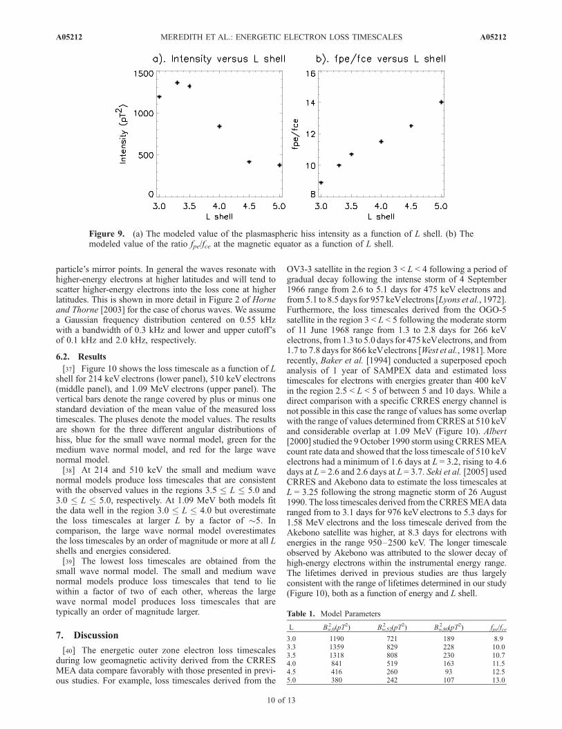
a function of L shell by averaging the intensities duringquiet conditions in steps of 0.2L first over magnetic latitudeand then over magnetic local time. The model wavemagnetic field intensities are plotted as a function of Lshell in Figure 9a and included in the second column ofTable 1. The model intensities have a peak value of1359 pT2 at L = 3.3 falling to 1190 pT2 at L = 3.0 and380 pT2 at L = 5.0.[33] The mean value of the ratio of fpe/fce is plotted as a

function of magnetic latitude for the same conditions andregions in the bottom panels of Figure 8. Along any given Lshell the ratio fpe/fce tends to decrease with increasing

latitude due to the increasing field strength with magneticlatitude. At a given magnetic latitude, the ratio fpe/fce tendsto increase with increasing L shell. The dashed lines showthe model values, determined from least squares best fits tothe data, assuming a dipole field and constant density. Theequatorial values of the best fit to fpe/fce are plotted as afunction of L shell in Figure 9b and are tabulated in the fifthcolumn of Table 1. The equatorial values of the ratio fpe/fceincrease from 8.9 at L = 3.0 to 13.0 at L = 5.0.[34] Plasmaspheric hiss appears to propagate over a broad

range of wave normal angles with predominantly field-aligned propagation near the geomagnetic equator andmore oblique propagation at higher latitudes [Parrot andLefeuvre, 1986; Hayakawa et al., 1986; Santolik et al.,2001]. For example, in the equatorial region (lm < 10�),Parrot and Lefeuvre [1986] found two populations of wavenormal angles, one lying in the range 0�� y� 30�, the otherin the range 40� � y � 60�. At higher latitudes (lm > 20�),most of the waves had larger wave normal angles in therange 55� � y � 85�. To investigate the effect of the wavenormal angle on the precipitation lifetimes, we use threedifferent angular distributions of hiss, chosen to be repre-sentative of these observations (Table 2).[35] The conversion from electric field intensity to mag-

netic field intensity assumes parallel propagation [Meredithet al., 2004]. We calculate approximate intensities forpropagation at 52� and 80� using the cold plasma dispersionsolver in the HOTRAY code [Horne, 1989] assuminga frequency of 0.55 kHz and using the modeled values offpe/fce. The derived intensities are tabulated in the third andfourth columns of Table 1 and are typically a factor of1.6 lower for a wave normal angle of 52� and a factor of5 lower for a wave normal angle of 80�.[36] We calculate the bounce-averaged diffusion rate

which takes into account the scattering of particles in pitchangle over the complete range of latitudes between the

Figure 7. The average hiss magnetic field wave intensityas a function of L and MLT for quiet conditions (Kp < 3�).The sampling distribution, color-coded to show the numberof minutes in each bin, tb(m), is shown in the small panel.

Figure 8. (top) The average hiss magnetic field wave intensity and (bottom) the ratio fpe/fce for quiettimes at different L shells. The model values are shown by the dashed lines.

A05212 MEREDITH ET AL.: ENERGETIC ELECTRON LOSS TIMESCALES

9 of 13

A05212

particle’s mirror points. In general the waves resonate withhigher-energy electrons at higher latitudes and will tend toscatter higher-energy electrons into the loss cone at higherlatitudes. This is shown in more detail in Figure 2 of Horneand Thorne [2003] for the case of chorus waves. We assumea Gaussian frequency distribution centered on 0.55 kHzwith a bandwidth of 0.3 kHz and lower and upper cutoff’sof 0.1 kHz and 2.0 kHz, respectively.

6.2. Results

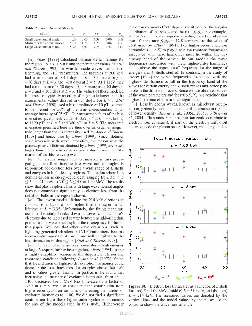
[37] Figure 10 shows the loss timescale as a function of Lshell for 214 keV electrons (lower panel), 510 keV electrons(middle panel), and 1.09 MeV electrons (upper panel). Thevertical bars denote the range covered by plus or minus onestandard deviation of the mean value of the measured losstimescales. The pluses denote the model values. The resultsare shown for the three different angular distributions ofhiss, blue for the small wave normal model, green for themedium wave normal model, and red for the large wavenormal model.[38] At 214 and 510 keV the small and medium wave

normal models produce loss timescales that are consistentwith the observed values in the regions 3.5 � L � 5.0 and3.0 � L � 5.0, respectively. At 1.09 MeV both models fitthe data well in the region 3.0 � L � 4.0 but overestimatethe loss timescales at larger L by a factor of �5. Incomparison, the large wave normal model overestimatesthe loss timescales by an order of magnitude or more at all Lshells and energies considered.[39] The lowest loss timescales are obtained from the

small wave normal model. The small and medium wavenormal models produce loss timescales that tend to liewithin a factor of two of each other, whereas the largewave normal model produces loss timescales that aretypically an order of magnitude larger.

7. Discussion

[40] The energetic outer zone electron loss timescalesduring low geomagnetic activity derived from the CRRESMEA data compare favorably with those presented in previ-ous studies. For example, loss timescales derived from the

OV3-3 satellite in the region 3 < L < 4 following a period ofgradual decay following the intense storm of 4 September1966 range from 2.6 to 5.1 days for 475 keV electrons andfrom5.1 to 8.5 days for 957 keVelectrons [Lyons et al., 1972].Furthermore, the loss timescales derived from the OGO-5satellite in the region 3 < L < 5 following the moderate stormof 11 June 1968 range from 1.3 to 2.8 days for 266 keVelectrons, from1.3 to 5.0 days for 475 keVelectrons, and from1.7 to 7.8 days for 866 keVelectrons [West et al., 1981]. Morerecently, Baker et al. [1994] conducted a superposed epochanalysis of 1 year of SAMPEX data and estimated losstimescales for electrons with energies greater than 400 keVin the region 2.5 < L < 5 of between 5 and 10 days. While adirect comparison with a specific CRRES energy channel isnot possible in this case the range of values has some overlapwith the range of values determined from CRRES at 510 keVand considerable overlap at 1.09 MeV (Figure 10). Albert[2000] studied the 9 October 1990 storm using CRRESMEAcount rate data and showed that the loss timescale of 510 keVelectrons had a minimum of 1.6 days at L = 3.2, rising to 4.6days at L = 2.6 and 2.6 days at L = 3.7. Seki et al. [2005] usedCRRES and Akebono data to estimate the loss timescales atL = 3.25 following the strong magnetic storm of 26 August1990. The loss timescales derived from the CRRESMEA dataranged from to 3.1 days for 976 keV electrons to 5.3 days for1.58 MeV electrons and the loss timescale derived from theAkebono satellite was higher, at 8.3 days for electrons withenergies in the range 950–2500 keV. The longer timescaleobserved by Akebono was attributed to the slower decay ofhigh-energy electrons within the instrumental energy range.The lifetimes derived in previous studies are thus largelyconsistent with the range of lifetimes determined in our study(Figure 10), both as a function of energy and L shell.

Figure 9. (a) The modeled value of the plasmaspheric hiss intensity as a function of L shell. (b) Themodeled value of the ratio fpe/fce at the magnetic equator as a function of L shell.

Table 1. Model Parameters

L Bw,02 (pT2) Bw,52

2 (pT2) Bw,802 (pT2) fpe/fce

3.0 1190 721 189 8.93.3 1359 829 228 10.03.5 1318 808 230 10.74.0 841 519 163 11.54.5 416 260 93 12.55.0 380 242 107 13.0

A05212 MEREDITH ET AL.: ENERGETIC ELECTRON LOSS TIMESCALES

10 of 13

A05212

[41] Albert [1999] calculated plasmaspheric lifetimes forthe region 1.5 < L < 5.0 using the parameter values of Abeland Thorne [1998] for whistler mode waves due to hiss,lightning, and VLF transmitters. The lifetimes at 200 keVhad a minimum of �14 days at L = 3.5, increasing to�50 days at L = 3 and �20 days at L = 5. At 1 MeV theyhad a minimum of �50 days at L = 3 rising to >400 days atL = 2 and �200 days at L = 5. The values of these modeledlifetimes are typically an order of magnitude larger than theexperimental values derived in our study. For L > 3, Abeland Thorne [1998] used a hiss amplitude of 10 pT assumedto be present for 50% of the time corresponding to anaverage intensity of 25 pT2. Our measured values of the hissintensities have a peak value of 1359 pT2 at L = 3.3, fallingto 1190 pT2 at L = 3 and 380 pT2 at L = 5. The measuredintensities presented here are thus over an order of magni-tude larger than the hiss intensity used by Abel and Thorne[1998] and hence also by Albert [1999]. Since lifetimesscale inversely with wave intensities, the reason why theplasmaspheric lifetimes obtained by Albert [1999] are muchlarger than the experimental values is due to an underesti-mation of the hiss wave power.[42] Our results suggest that plasmaspheric hiss propa-

gating at small or intermediate wave normal angles isresponsible for electron loss over a wide range of L shellsand energies in high-density regions. The region where hissdominates loss is energy-dependent, ranging from 3.5 � L� 5.0 at 214 keV to 3.0 � L � 4.0 at 1.09 MeV. The resultsshow that plasmaspheric hiss with large wave normal anglesdoes not contribute significantly to electron loss from theradiation belts in the regions shown.[43] The lowest model lifetime for 214 keV electrons at

L = 3.3 is a factor of �3 higher than the experimentallifetime at L = 3.35. Unfortunately, the fitting techniqueused in this study breaks down at lower L for 214 keVelectrons due to increased scatter between neighboring datapoints so that we cannot explore the discrepancy further inthis paper. We note that other wave emissions, such aslightning-generated whistlers and VLF transmitters, becomeincreasingly important at low L and will contribute to theloss timescales in this region [Abel and Thorne, 1998].[44] Our calculated larger loss timescales at high energies

at large L require further investigation. Albert [1994], usinga highly simplified version of the dispersion relation andresonance condition following Lyons et al. [1972], foundthat the inclusion of higher-order cyclotron harmonics coulddecrease the loss timescales, for energies above 500 keVand L values greater than 3. In particular, he found thatincreasing the number of cyclotron harmonics from ±5 to±100 decreased the 1 MeV loss timescale by a factor of�2.3 at L = 5. We also considered the contribution fromhigher-order cyclotron harmonics, increasing the number ofcyclotron harmonics to ±100. We did not find a significantcontribution from these higher-order cyclotron harmonicsfor any of the models used in this study. Higher-order

cyclotron resonant effects depend sensitively on the angulardistribution of the waves and the ratio fpe/fce. For example,at L = 5 our modeled equatorial value, based on observa-tions, for the ratio fpe/fce is 12.8 compared to the value of26.9 used by Albert [1994]. For higher-order cyclotronharmonics (jnj > 5) to play a role the resonant frequenciesassociated with these harmonics must lie within the fre-quency band of the waves. In our models the wavefrequencies associated with these higher-order harmonicsall lie above the upper cutoff frequency for the range ofenergies and L shells studied. In contrast, in the study ofAlbert [1994] the wave frequencies associated with thehigher-order harmonics fall in the frequency band of thewaves for certain energy and L shell ranges and hence playa role in the diffusion process. Since we use observed valuesof the wave parameters and the ratio fpe/fce, we conclude thathigher harmonic effects are not significant.[45] Loss by chorus waves, known as microburst precip-

itation, generally occurs outside the plasmapause in regionsof lower density [Thorne et al., 2005a, 2005b; O’Brien etal., 2004]. Thus microburst precipitation could contribute toelectron loss at large L if part of the electron drift orbitoccurs outside the plasmapause. However, modeling studies

Table 2. Wave Normal Models

Model y Xm dX Xlc Xuc

Small wave normal model 0.0 0.00 0.36 0.00 0.58Medium wave normal model 52.0 1.28 0.27 0.84 1.73Large wave normal model 80.0 5.67 2.74 1.43 11.4

Figure 10. Electron loss timescales as a function of L shellfor (top) E = 1.09 MeV, (middle) E = 510 keV, and (bottom)E = 214 keV. The measured values are denoted by thevertical lines and the model values by the pluses, color-coded to show the wave normal angle.

A05212 MEREDITH ET AL.: ENERGETIC ELECTRON LOSS TIMESCALES

11 of 13

A05212

show that as chorus propagates along the magnetic field theresonant energies match � MeV electrons at 20�–30� offthe equator and are not well matched at the equator [Horneand Thorne, 2003]. At the equator the resonant energies arelower. Thus one may expect that if microburst precipitationwere occurring, this would also reduce the loss timescales atlower energies. It appears that plasmaspheric hiss is ade-quate to explain the loss at lower energies. This does notrule out microburst loss provided the rate of loss at lowerenergies is dominated by hiss.[46] EMIC waves can interact with MeV electrons [e.g.,

Summers and Thorne, 2003; Albert, 2003; Summers, 2005],particularly in regions of high density at larger L (L > 4.5)[Meredith et al., 2003c], precisely the region where theMeV losses cannot be explained by resonant interactionswith plasmaspheric hiss alone. Furthermore, Albert [2003]found that the addition of EMIC waves can greatly reducethe electron lifetimes determined by hiss alone. In addition,precipitation signatures from EMIC waves have been seenin plumes during substorm ion injections. These resultssuggest that EMIC waves in high-density regions, such asthe duskside plasmapause and within drainage plumes, maycontribute to the scattering of energetic electrons at larger L,and could, potentially, explain the loss rates in this region.

8. Conclusions

[47] We have analyzed CRRES particle data to determinethe energetic electron decay timescales as a function ofenergy (214 keV � E � 1.09 MeV) and L shell (3 � L � 5).The resulting timescales are compared with estimates of thedecay timescales of plasmaspheric hiss using the PADIEcode using CRRES wave data as input. Our principal resultsare as follows:[48] 1. Gradual loss of energetic electrons in the region

3 � L � 5 is observed to occur in quiet periods (Kp < 3�)following enhanced magnetic activity.[49] 2. Decay timescales range from 1.5–3.5 days for

214 keV electrons to 5.5–6.5 days for 1.09 MeV electrons.[50] 3. The intervals of decay are associated with large

average values of the ratio fpe/fce (>7) and indicate that thedecay takes place in the plasmasphere.[51] 4. Modeling shows that plasmaspheric hiss propa-

gating at small or intermediate wave normal angles canaccount for the electron loss rates over a wide range ofenergies and L shells. These regions are energy-dependentand range from 3.5 � L � 5.0 at 214 keV to 3.0 � L � 4.0at 1.09 MeV.[52] 5. Modeling shows that plasmaspheric hiss with very

large wave normal angles does not contribute significantlyto radiation belt electron loss.[53] 6. At high energies, E = 1.09MeV, plasmaspheric hiss

propagating at small or intermediate wave normal anglesoverestimates the loss timescales by a factor of �5 at large L(4.5 � L � 5.0). Resonant wave-particle interactions withEMIC waves become important at MeV energies at larger Land high densities.We suggest that losses due to EMICwavesmay play a significant role at larger L.

[54] Acknowledgments. We thank Al Vampola and Daniel Heynder-ickx for providing the MEA data used in this study and for many usefuldiscussions. We also thank the NSSDC Omniweb for providing the Kpindices used in this paper. This work was supported in part by NSF grant

ATM0402615 and NASA grant NNG04GN44G. D.S. acknowledges sup-port from the Natural Sciences and Engineering Research Council ofCanada under grant A-0621.[55] Shadia Rifai Habbal thanks Takahiro Obara for his assistance in

evaluating this paper.

ReferencesAbel, B., and R. M. Thorne (1998), Electron scattering loss in the Earth’sinner magnetosphere: 1. Dominant physical processes, J. Geophys. Res.,103, 2385.

Albert, J. M. (1994), Quasi-linear pitch-angle diffusion coefficients: Retain-ing higher harmonics, J. Geophys. Res., 99, 23,741.

Albert, J. M. (1999), Analysis of quasi-linear diffusion coefficients,J. Geophys. Res., 104, 2429.

Albert, J. M. (2000), Pitch-angle diffusion as seen by CRRES, Adv. SpaceRes., 25, 2343.

Albert, J. M. (2003), Evaluation of quasi-linear diffusion coefficients forEMIC waves in a multispecies plasma, J. Geophys. Res., 108(A6), 1249,doi:10.1029/2002JA009792.

Anderson, R. R., D. A. Gurnett, and D. L. Odem (1992), CRRES plasmawave experiment, J. Spacecr. Rockets, 29, 570.

Baker, D. (2001), Satellite anomalies due to space storms, in Space Stormsand Space Weather Hazards, edited by I. A. Daglis, pp. 251–284, chap.10, Springer, New York.

Baker, D. N., J. B. Blake, R. W. Klebesadel, and P. R. Higbie (1986),Highly relativistic electrons in the Earth’s outer magnetosphere: 1. Life-times and temporal history 1979–1984, J. Geophys. Res., 91, 4265.

Baker, D. N., J. B. Blake, L. B. Callis, J. R. Cummings, D. Hovestadt,S. Kanekal, B. Blecker, R. A. Mewaldt, and R. D. Zwickl (1994),Relativistic electron acceleration and decay timescales in the inner andouter radiation belts: SAMPEX, Geophys. Res. Lett., 21, 409.

Baker, D. N., et al. (1997), Recurrent geomagnetic storms and relativisticelectron enhancements in the outer magnetosphere: ISTP coordinatedmeasurements, J. Geophys. Res., 102, 14,141.

Baker, D. N., J. H. Allen, S. G. Kanekal, and G. D. Reeves (1998a),Disturbed space environment may have been related to pager satellitefailure, Eos Trans. AGU, 79, 477.

Baker, D. N., X. Li, J. B. Blake, and S. G. Kanekal (1998b), Strong electronacceleration in the Earth’s magnetosphere, Adv. Space. Res., 21, 609.

Callis, L. B., M. Natarajan, J. D. Lambeth, and D. N. Baker (1998),Solar atmospheric coupling by electrons (SOLACE): 2. Calculatedstratospheric effects of precipitating electrons, J. Geophys. Res., 103,28,421.

Carpenter, D. L., and R. R. Anderson (1992), An ISEE/whistler model ofequatorial electron density in the magnetosphere, J. Geophys. Res., 97,1097.

Elkington, S. R., M. K. Hudson, and A. A. Chan (1999), Acceleration ofrelativistic electrons via drift resonant interactions with torroidal-modePc-5 ULF oscillations, Geophys. Res. Lett., 26, 3273.

Friedel, R. H. W., G. D. Reeves, and T. Obara (2002), Relativistic electrondynamics in the inner magnetosphere—A review, J. Atmos. Sol. Terr.Phys., 64, 265.

Glauert, S. A., and R. B. Horne (2005), Calculation of pitch angle andenergy diffusion coefficients with the PADIE code, J. Geophys. Res.,110, A04206, doi:10.1029/2004JA010851.

Hayakawa, M., M. Parrot, and F. Lefeuvre (1986), The wave normals ofELF hiss emissions observed onboard GEOS 1 at the equatorial and off-equatorial regions of the plasmasphere, J. Geophys. Res., 91, 7989.

Horne, R. B. (1989), Path-integrated growth of electrostatic waves: Thegeneration of terrestrial myriametric radiation, J. Geophys. Res., 94,8895.

Horne, R. B. (2002), The contribution of wave particle interactions toelectron loss and acceleration in the Earth’s radiation belts during geo-magnetic storms, in Review of Radio Science 1999–2002, edited by W. R.Stone, pp. 801–828, chap. 33, John Wiley, Hoboken, N. J.

Horne, R. B., and R. M. Thorne (2003), Relativistic electron accelerationand precipitation during resonant interactions with whistler mode chorus,Geophys. Res. Lett., 30(10), 1527, doi:10.1029/2003GL016973.

Horne, R. B., S. A. Glauert, and R. M. Thorne (2003), Resonant diffusionof radiation belt electrons by whistler mode chorus, Geophys. Res. Lett.,30(9), 1493, doi:10.1029/2003GL016963.

Horne, R. B., N. P. Meredith, S. A. Glauert, A. Varotsou, R. M. Thorne,Y. Y. Shprits, and R. R. Anderson (2006), Mechanisms for the accelera-tion of radiation belt electrons, in The Solar Wind: Corotating Streamsand Recurrent Geomagnetism, Geophys. Monogr. Ser., vol. 167, editedby B. T. Tsurutani et al., in press.

Hudson, M. K., S. R. Elkington, J. G. Lyon, V. A. Machenko, I. Roth,M. Temerin, J. B. Blake, M. S. Gussenhoven, and J. R. Wygant (1997),Simulation of radiation belt formation during sudden storm commence-ments, J. Geophys. Res., 102, 14,087.

A05212 MEREDITH ET AL.: ENERGETIC ELECTRON LOSS TIMESCALES

12 of 13

A05212

Hudson, M. K., S. R. Elkington, J. G. Lyon, and C. C. Goodrich (2000),Increase in relativistic electron flux in the inner magnetosphere: ULFwave mode structure, Adv. Space Res., 25, 2327.

Johnson, M. H., and J. Kierein (1992), Combined Release and RadiationEffects Satellite (CRRES): Spacecraft and mission, J. Spacecr. Rockets,29, 556.

Lastovicka, J. (1996), Effects of geomagnetic storms in the lower iono-sphere, middle atmosphere and troposphere, J. Atmos. Terr. Phys., 58,831.

Li, X., and M. A. Temerin (2001), The electron radiation belt, Space Sci.Rev., 95, 569.

Li, X., I. Roth, M. Temerin, J. Wygant, M. K. Hudson, and J. B. Blake(1993), Simulation of prompt energization, and transport of radiation beltparticles during the March 23, 1991 SSC, Geophys. Res. Lett., 20, 2423.

Li, X., D. N. Baker, M. Temerin, T. E. Cayton, G. D. Reeves, R. A.Christiansen, J. B. Blake, M. D. Looper, R. Nakamura, and S. G. Kanekal(1997), Multi-satellite observations of the outer zone electron variationduring the November 3–4, 1993, magnetic storm, J. Geophys. Res., 102,14,123.

Liu, W. W., G. Rostoker, and D. N. Baker (1999), Internal acceleration ofrelativistic electrons by large amplitude ULF pulsations, J. Geophys.Res., 104, 17,391.

Lyons, L. R., R. M. Thorne, and C. F. Kennel (1972), Pitch-angle diffusionof radiation belt electrons within the plasmasphere, J. Geophys. Res., 77,3455.

Meredith, N. P., R. B. Horne, and R. R. Anderson (2001), Substorm de-pendence of chorus amplitudes: Implications for the acceleration of elec-trons to relativistic energies, J. Geophys. Res., 106, 13,165.

Meredith, N. P., R. B. Horne, R. H. A. Iles, R. M. Thorne, R. R. Anderson,and D. Heynderickx (2002a), Outer zone relativistic electron accelerationassociated with substorm enhanced whistler mode chorus, J. Geophys.Res., 107(A7), 1144, doi:10.1029/2001JA900146.

Meredith, N. P., R. B. Horne, D. Summers, R. M. Thorne, R. H. A. Iles,D. Heynderickx, and R. R. Anderson (2002b), Evidence for accelerationof outer zone electrons to relativistic energies by whistler mode chorus,Ann. Geophys., 20, 967.

Meredith, N. P., R. B. Horne, R. M. Thorne, and R. R. Anderson (2003a),Favored regions for chorus-driven electron acceleration to relativisticenergies in the Earth’s outer radiation belt, Geophys. Res. Lett., 30(16),1871, doi:10.1029/2003GL017698.

Meredith, N. P., M. Cain, R. B. Horne, R. M. Thorne, D. Summers, andR. R. Anderson (2003b), Evidence for chorus driven electron accelera-tion to relativistic energies from a survey of geomagnetically disturbedperiods, J. Geophys. Res., 108(A6), 1248, doi:10.1029/2002JA009764.

Meredith, N. P., R. M. Thorne, R. B. Horne, D. Summers, B. J. Fraser, andR. R. Anderson (2003c), Statistical analysis of relativistic electron en-ergies for cyclotron resonance with EMIC waves observed on CRRES,J. Geophys. Res., 108(A6), 1250, doi:10.1029/2002JA009700.

Meredith, N. P., R. B. Horne, R. M. Thorne, D. Summers, and R. R.Anderson (2004), Substorm dependence of plasmaspheric hiss, J. Geo-phys. Res., 109, A06209, doi:10.1029/2004JA010387.

Miyoshi, Y., A. Morioka, T. Obara, H. Misawa, T. Nagai, and Y. Kasahara(2003), Rebuilding process of the outer radiation belt during the Novem-ber 3, 1993, magnetic storm: NOAA and EXOS-D observations, J. Geo-phys. Res., 108(A1), 1004, doi:10.1029/2001JA007542.

Obara, T., T. Nagatsuma, M. Den, Y. Miyoshi, and A. Morioka (2000),Main phase creation of ‘‘seed’’ electrons in the outer radiation belt, EarthPlanets Space, 52, 41.

O’Brien, T. P., K. R. Lorentzen, I. R. Mann, N. P. Meredith, J. B. Blake,J. F. Fennel, M. D. Looper, D. K. Milling, and R. R. Anderson (2003),Energization of relativistic electrons in the presence of ULF power andMeV microbursts: Evidence for dual ULF and VLF acceleration,J. Geophys. Res., 108(A3), 1329, doi:10.1029/2002JA009784.

O’Brien, T. P., M. D. Looper, and J. B. Blake (2004), Quantification ofrelativistic electron microbursts losses during the GEM storms, Geophys.Res. Lett., 31, L04802, doi:10.1029/2003GL018621.

Paulikas, G. A., and J. B. Blake (1979), Effects of the solar wind onmagnetospheric dynamics: Energetic electrons at synchronous orbit, inQuantitative Modeling of Magnetospheric Processes, Geophys. Monogr.Ser., vol. 21, edited by W. P. Olsen, p. 180, AGU, Washington D. C.

Parrot, M., and F. Lefeuvre (1986), Statistical study of the propagationcharacteristics of ELF hiss observed on GEOS-1, inside and outsidethe plasmasphere, Ann. Geophys., 4, 363.

Reeves, G. D., R. H. W. Friedel, R. D. Belian, M. M. Meiet, M. G.Henderson, T. Onsager, H. J. Singer, D. N. Baker, X. Li, and J. B. Blake

(1998), The relativistic electron response at geosynchronous orbit duringthe January 1997 magnetic storm, J. Geophys. Res., 103, 17,559.

Santolik, O., M. Parrot, L. R. O. Storey, J. S. Pickett, and D. A. Gurnett(2001), Propagation analysis of plasmaspheric hiss using Polar PWImeasurements, Geophys. Res. Lett., 28, 1127.

Seki, K., Y. Miyoshi, D. Summers, and N. P. Meredith (2005), Comparativestudy of outer-zone relativistic electrons observed by Akebono andCRRES, J. Geophys. Res., 110, A02203, doi:10.1029/2004JA010655.

Sheeley, B. W., M. B. Moldwin, H. K. Rassoul, and R. R. Anderson (2001),An empirical plasmasphere and trough density model: CRRES observa-tions, J. Geophys. Res., 106, 25,631.

Smith, E. J., A. M. Frandsen, B. T. Tsurutani, R. M. Thorne, and K. W.Chan (1974), Plasmaspheric hiss intensity variations during magneticstorms, J. Geophys. Res., 79, 2507.

Summers, D. (2005), Quasi-linear diffusion coefficients for field-alignedelectromagnetic waves with application to the magnetosphere, J. Geo-phys. Res., 110, A08213, doi:10.1029/2005JA011159.

Summers, D., and R. M. Thorne (2003), Relativistic electron pitch-anglescattering by electromagnetic ion cyclotron waves during geomagneticstorms, J. Geophys. Res., 108(A4), 1143, doi:10.1029/2002JA009489.

Summers, D., R. M. Thorne, and F. Xiao (1998), Relativistic theory ofwave-particle resonant diffusion with application to electron accelerationin the magnetosphere, J. Geophys. Res., 103, 20,487.

Summers, D., C. Ma, and T. Mukai (2004), Competition between accelera-tion and loss mechanisms of relativistic electrons during geomagneticstorms, J. Geophys. Res., 109, A04221, doi:10.1029/2004JA010437.

Summers, D., R. L. Mace, and M. A. Hellberg (2005), Pitch-angle scatter-ing rates in planetary magnetospheres, J. Plasma Phys., 71, 237.

Thorne, R. M. (1980), The importance of energetic particle precipitation onthe chemical composition of the middle atmosphere, Pure Appl. Geo-phys., 118, 128.

Thorne, R. M., E. J. Smith, R. K. Burton, and R. E. Holzer (1973), Plasma-spheric hiss, J. Geophys. Res., 78, 1581.

Thorne, R. M., S. R. Church, W. J. Malloy, and B. T. Tsurutani (1977), Thelocal time variation of ELF emissions during periods of substorm activity,J. Geophys. Res., 82, 1585.

Thorne, R. M., T. P. O’Brien, Y. Y. Shprits, D. Summers, and R. B. Horne(2005a), Timescale for MeVelectron microburst loss during geomagneticstorms, J. Geophys. Res., 110, A09202, doi:10.1029/2004JA010882.

Thorne, R. M., R. B. Horne, S. A. Glauert, N. P. Meredith, Y. Shprits,D. Summers, and R. R. Anderson (2005b), The influence of wave-particleinteractions on relativistic electron dynamics during storms, in InnerMagnetosphere Interactions: New Perspectives From Imaging, Geophys.Monogr. Ser., vol. 159, edited by J. Burch, M. Schulz, and H. Spence,p. 101, AGU, Washington, D. C.

Tsurutani, B. T., and E. J. Smith (1977), Two types of magnetospheric ELFchorus and their substorm dependencies, J. Geophys. Res., 82, 5112.

Vampola, A. L., J. V. Osborn, and B. M. Johnson (1992), CRRES magneticelectron spectrometer, J. Spacecr. Rockets, 29, 592.

Varotsou, A., D. Boscher, S. Bourdarie, R. B. Horne, S. A. Glauert, andN. P. Meredith (2005), Simulation of the outer radiation belt electronsnear geosynchronous orbit including both radial diffusion and resonantinteraction with whistler mode chorus waves, Geophys. Res. Lett., 32,L19106, doi:10.1029/2005GL023282.

West, H. I., R. M. Buck, and G. T. Davidson (1981), The dynamics ofenergetic electrons in the Earth’s outer radiation belt during 1968 asobserved by the Lawrence Livermore National Laboratory’s Spectrometeron Ogo 5, J. Geophys. Res., 86, 2111.

�����������������������J. M. Albert, Air Force Research Laboratory/VSBX, 29 Randolph Road,

Hanscom Air Force Base, MA 01731-3010, USA. (jay.albert@hanscom.af.mil)R. R. Anderson, Department of Physics and Astronomy, University of

Iowa, IowaCity, Iowa, IA 52242-1479,USA. (roger-r-anderson@uiowa.edu)S. A. Glauert, R. B. Horne, and N. P. Meredith, British Antarctic Survey,

Natural Environment Research Council, Madingley Road, Cambridge, CB30ET, UK. (sagl@bas.ac.uk; r.horne@bas.ac.uk; nmer@bas.ac.uk)D. Summers, Department of Mathematics and Statistics, Memorial

University of Newfoundland, St John’s, Newfoundland, Canada, A1C 5S7.(dsummers@math.mun.ca)R. M. Thorne, Department of Atmospheric and Oceanic Sciences,

University of California, Los Angeles, 405 Hilgard Avenue, Los Angeles,CA 90095-1565, USA. (rmt@atmos.ucla.edu)

A05212 MEREDITH ET AL.: ENERGETIC ELECTRON LOSS TIMESCALES

13 of 13

A05212