Embed Size (px)
Citation preview
Energetic (>10keV) and relativistic electron (>500keV) precipitation into the mesosphere
- evidence and limitations
Craig J. Rodger
Department of Physics
University of Otago
Dunedin
NEW ZEALAND
HEPPA/SOLARIS 2012
Energetic particle measurements 10:45-11:15 Wednesday 10 October 2012
Craig J. Rodger1, and M. A. Clilverd2
1. Physics Department, University of Otago, Dunedin, New Zealand.
2. British Antarctic Survey (NERC), Cambridge, United Kingdom.
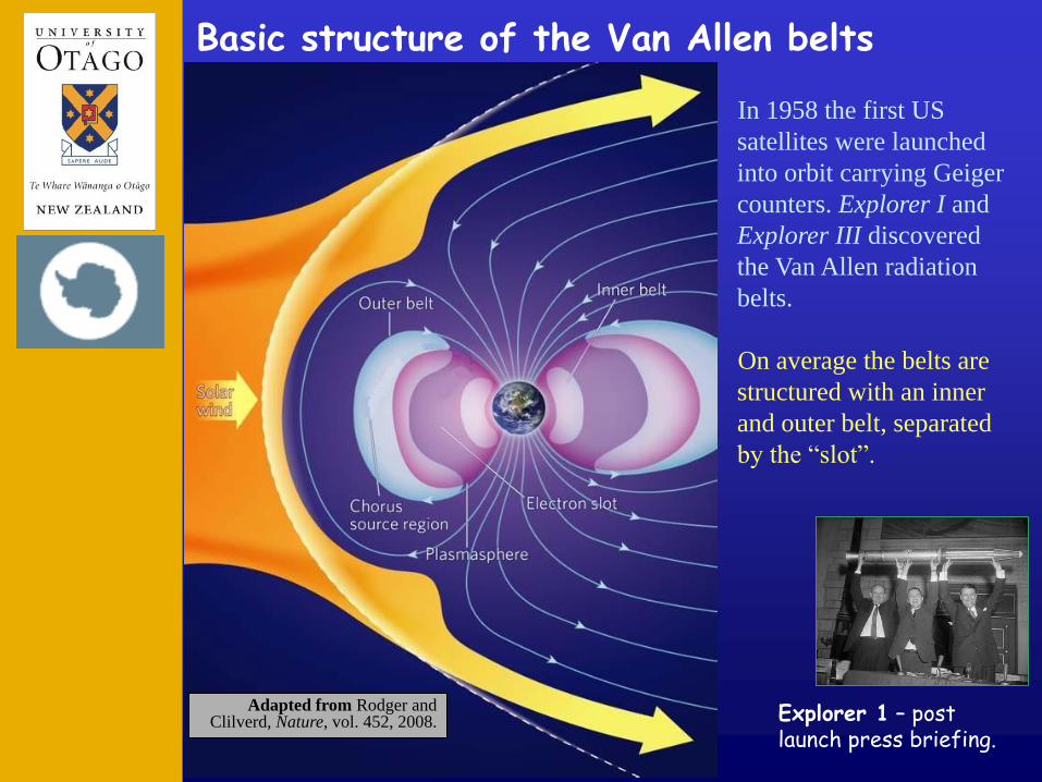
Basic structure of the Van Allen belts
In 1958 the first US
satellites were launched
into orbit carrying Geiger
counters. Explorer I and
Explorer III discovered
the Van Allen radiation
belts.
On average the belts are
structured with an inner
and outer belt, separated
by the “slot”.
Adapted from Rodger and Clilverd, Nature, vol. 452, 2008. Explorer 1 – post
launch press briefing.
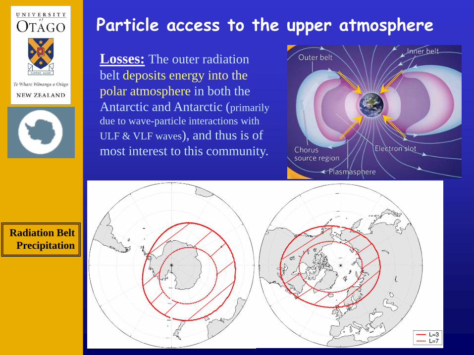
Particle access to the upper atmosphere
Radiation Belt
Precipitation
Losses: The outer radiation
belt deposits energy into the
polar atmosphere in both the
Antarctic and Antarctic (primarily
due to wave-particle interactions with
ULF & VLF waves), and thus is of
most interest to this community.
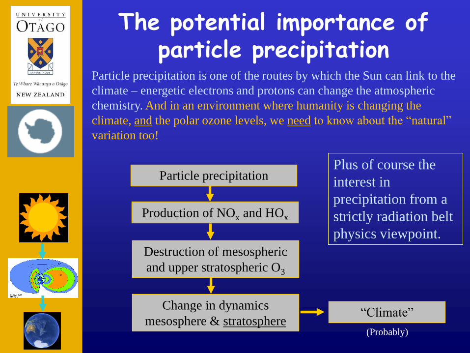
The potential importance of particle precipitation
Particle precipitation is one of the routes by which the Sun can link to the
climate – energetic electrons and protons can change the atmospheric
chemistry. And in an environment where humanity is changing the
climate, and the polar ozone levels, we need to know about the “natural”
variation too!
Particle precipitation
Production of NOx and HOx
Change in dynamics
mesosphere & stratosphere
Destruction of mesospheric
and upper stratospheric O3
“Climate”
Plus of course the
interest in
precipitation from a
strictly radiation belt
physics viewpoint.
(Probably)
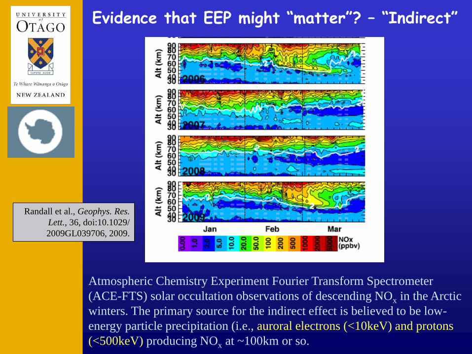
Atmospheric Chemistry Experiment Fourier Transform Spectrometer
(ACE-FTS) solar occultation observations of descending NOx in the Arctic
winters. The primary source for the indirect effect is believed to be low-
energy particle precipitation (i.e., auroral electrons (<10keV) and protons
(<500keV) producing NOx at ~100km or so.
Randall et al., Geophys. Res.
Lett., 36, doi:10.1029/
2009GL039706, 2009.
Evidence that EEP might “matter”? – “Indirect”

NO observations from the British Antarctic Survey radiometer located
at Troll station, Antarctica (65° geomagnetic latitude). NO increases at
~75km by 2-3 orders of magnitude due to multiple days of ~300keV
precipitation. This effect is far too fast to explain through transport.
Newnham et al., Geophys.
Res. Lett.,
doi:10.1029/2011GL049199,
2011.
Evidence that EEP might “matter”? – “Direct” (NOx)

Correlation between POES satellite precipitating electron count rates and OH
(part of the HOx family). In one third of the months from 2004-2009 the
observed OH variation is best explained by EEP, with direct OH-increases
measured to as low as 52 km altitude (~3MeV electrons!).
Andersson et al. (2012),
J. Geophys. Res.,
10.1029/2011JD01724.
Evidence that EEP might “matter”? – “Direct” (HOx)

+
Evidence that EEP might “matter”? – “Direct” (O3)
AARDDVARK subionospheric VLF observations DEMETER DLC
Precipitation fluxes required to reproduce the changes in AARDDVARK-observed subionospheric propagation (NAA -> CAM).
Peak Fluxes:
8000 el. cm-2s-1 at midday
800 cm-2s-1 at midnight.
Rodger et al. (2010), J.
Geophys. Res.,
10.1029/2010JA015599.
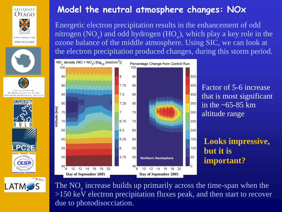
Model the neutral atmosphere changes: NOx
Energetic electron precipitation results in the enhancement of odd nitrogen (NOx) and odd hydrogen (HOx), which play a key role in the ozone balance of the middle atmosphere. Using SIC, we can look at the electron precipitation produced changes, during this storm period.
Factor of 5-6 increase that is most significant in the ~65-85 km altitude range
The NOx increase builds up primarily across the time-span when the >150 keV electron precipitation fluxes peak, and then start to recover due to photodisocciation.
Looks impressive, but it is
important?
Day of September 2005 Day of September 2005
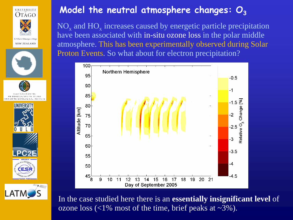
Model the neutral atmosphere changes: O3
NOx and HOx increases caused by energetic particle precipitation have been associated with in-situ ozone loss in the polar middle atmosphere. This has been experimentally observed during Solar Proton Events. So what about for electron precipitation?
In the case studied here there is an essentially insignificant level of ozone loss (<1% most of the time, brief peaks at ~3%).
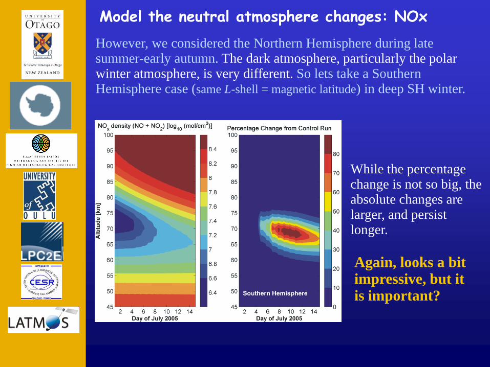
Model the neutral atmosphere changes: NOx
However, we considered the Northern Hemisphere during late summer-early autumn. The dark atmosphere, particularly the polar winter atmosphere, is very different. So lets take a Southern Hemisphere case (same L-shell = magnetic latitude) in deep SH winter.
While the percentage change is not so big, the absolute changes are larger, and persist longer.
Again, looks a bit impressive, but it
is important?
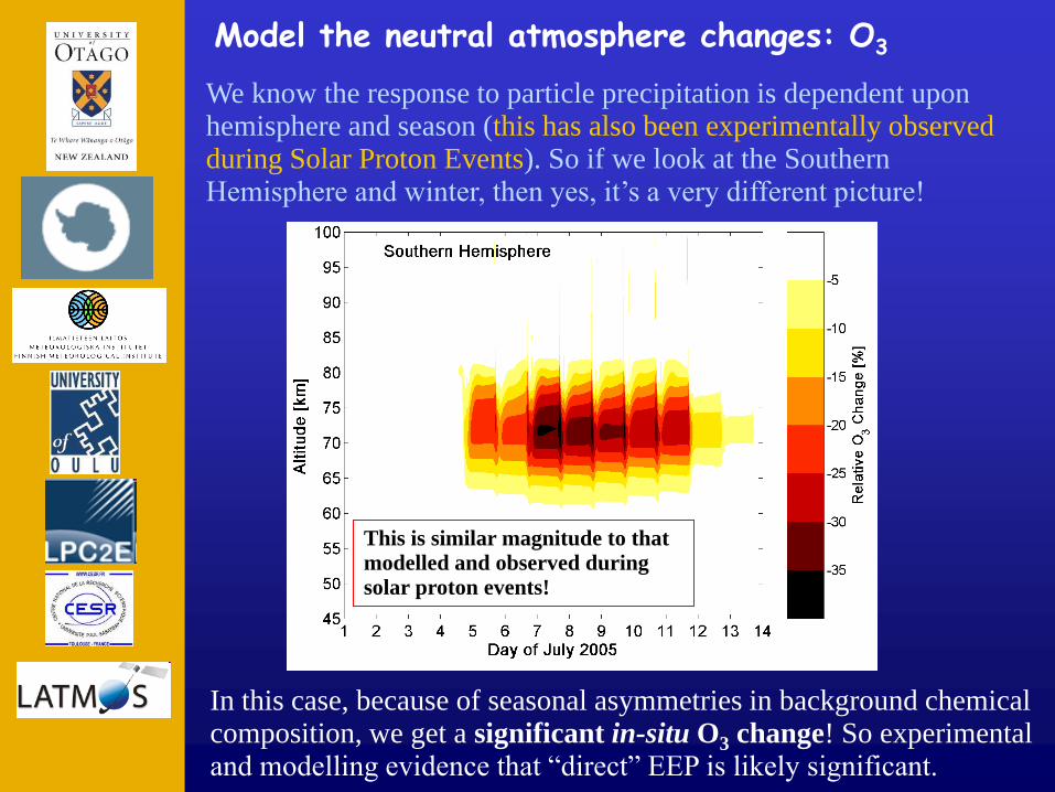
Model the neutral atmosphere changes: O3
We know the response to particle precipitation is dependent upon hemisphere and season (this has also been experimentally observed during Solar Proton Events). So if we look at the Southern Hemisphere and winter, then yes, it’s a very different picture!
In this case, because of seasonal asymmetries in background chemical composition, we get a significant in-situ O3 change! So experimental and modelling evidence that “direct” EEP is likely significant.
This is similar magnitude to that modelled and observed during solar proton events!
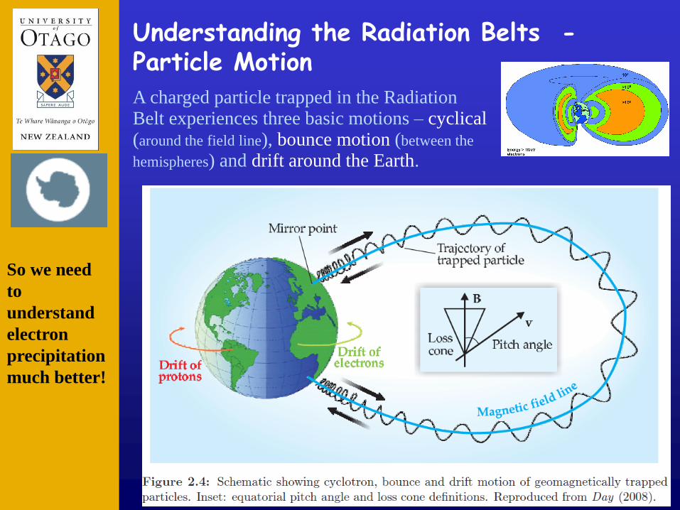
Understanding the Radiation Belts - Particle Motion A charged particle trapped in the Radiation Belt experiences three basic motions – cyclical (around the field line), bounce motion (between the
hemispheres) and drift around the Earth.
So we need
to
understand
electron
precipitation
much better!
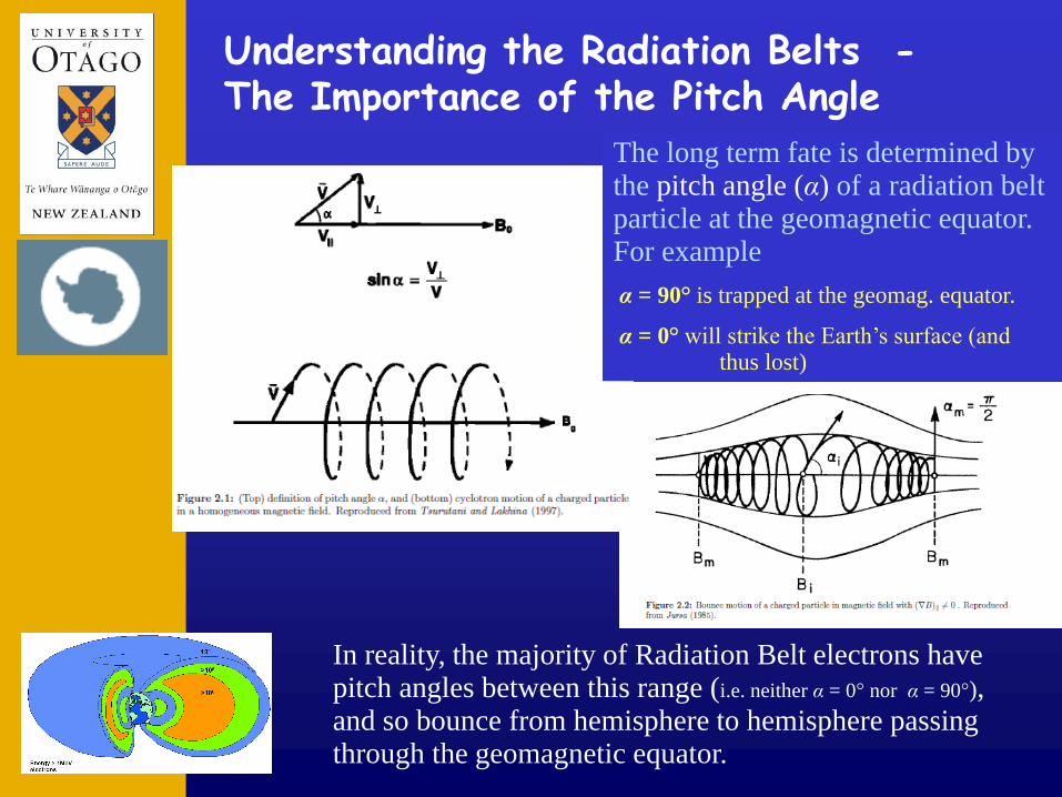
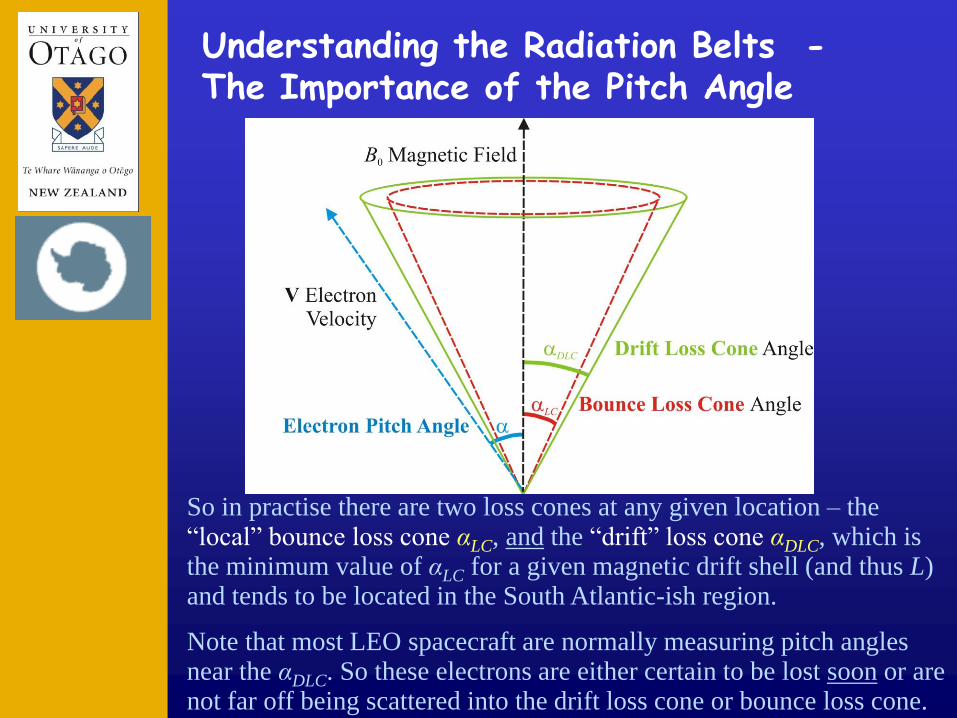
Understanding the Radiation Belts -The Importance of the Pitch Angle
The long term fate is determined by the pitch angle (α) of a radiation belt particle at the geomagnetic equator. For example
α = 90° is trapped at the geomag. equator.
α = 0° will strike the Earth’s surface (and thus lost)
In reality, the majority of Radiation Belt electrons have pitch angles between this range (i.e. neither α = 0° nor α = 90°), and so bounce from hemisphere to hemisphere passing through the geomagnetic equator.
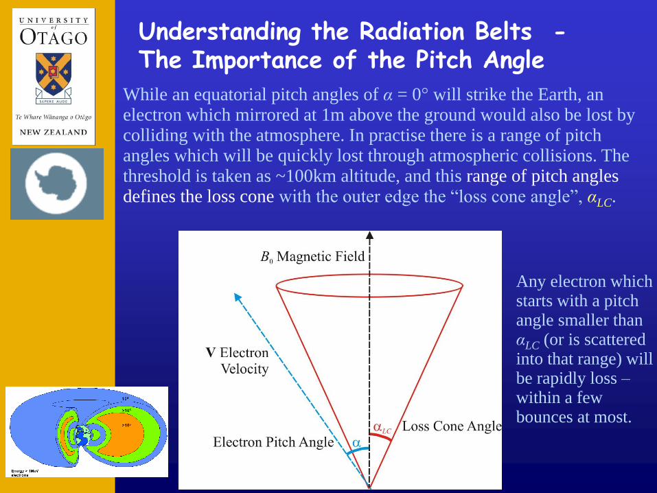
Understanding the Radiation Belts -The Importance of the Pitch Angle
While an equatorial pitch angles of α = 0° will strike the Earth, an electron which mirrored at 1m above the ground would also be lost by colliding with the atmosphere. In practise there is a range of pitch angles which will be quickly lost through atmospheric collisions. The threshold is taken as ~100km altitude, and this range of pitch angles defines the loss cone with the outer edge the “loss cone angle”, αLC.
Any electron which starts with a pitch angle smaller than αLC (or is scattered into that range) will be rapidly loss – within a few bounces at most.
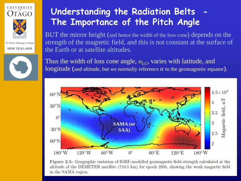
Understanding the Radiation Belts -The Importance of the Pitch Angle
BUT the mirror height (and hence the width of the loss cone) depends on the strength of the magnetic field, and this is not constant at the surface of the Earth or at satellite altitudes.
Thus the width of loss cone angle, αLC, varies with latitude, and longitude (and altitude, but we normally reference α to the geomagnetic equator).
SAMA (or
SAA)
Understanding the Radiation Belts -The Importance of the Pitch Angle
So in practise there are two loss cones at any given location – the “local” bounce loss cone αLC, and the “drift” loss cone αDLC, which is the minimum value of αLC for a given magnetic drift shell (and thus L) and tends to be located in the South Atlantic-ish region.
Note that most LEO spacecraft are normally measuring pitch angles near the αDLC. So these electrons are either certain to be lost soon or are not far off being scattered into the drift loss cone or bounce loss cone.
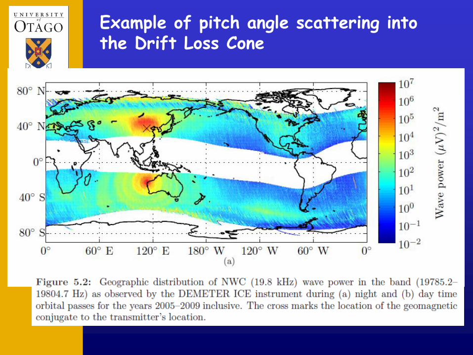
Example of pitch angle scattering into the Drift Loss Cone
NWC
Dunedin
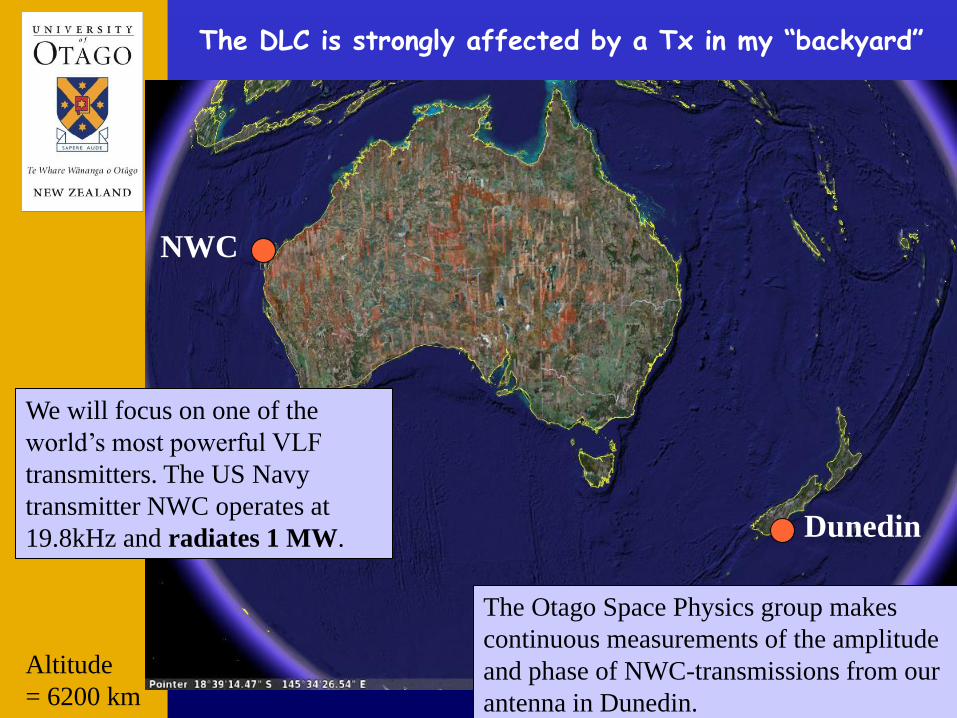
We will focus on one of the
world’s most powerful VLF
transmitters. The US Navy
transmitter NWC operates at
19.8kHz and radiates 1 MW.
The Otago Space Physics group makes
continuous measurements of the amplitude
and phase of NWC-transmissions from our
antenna in Dunedin.
The DLC is strongly affected by a Tx in my “backyard”
Altitude
= 6200 km
Altitude
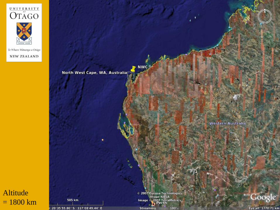
= 1800 km
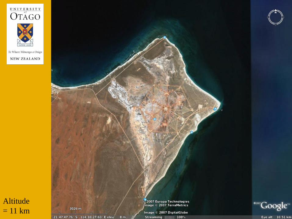
Altitude
= 11 km
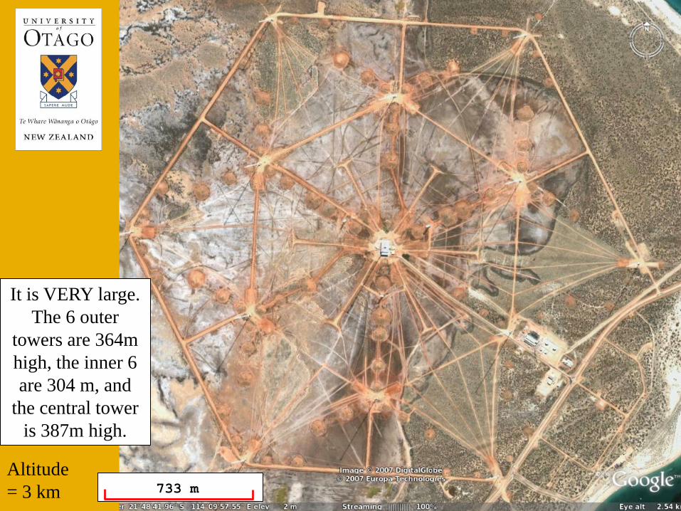
733 m
It is VERY large.
The 6 outer
towers are 364m
high, the inner 6
are 304 m, and
the central tower
is 387m high.
Altitude
= 3 km
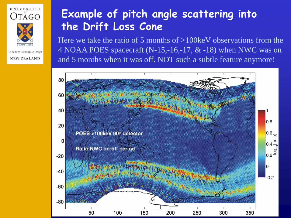
Here we take the ratio of 5 months of >100keV observations from the
4 NOAA POES spacecraft (N-15,-16,-17, & -18) when NWC was on
and 5 months when it was off. NOT such a subtle feature anymore!
Example of pitch angle scattering into the Drift Loss Cone
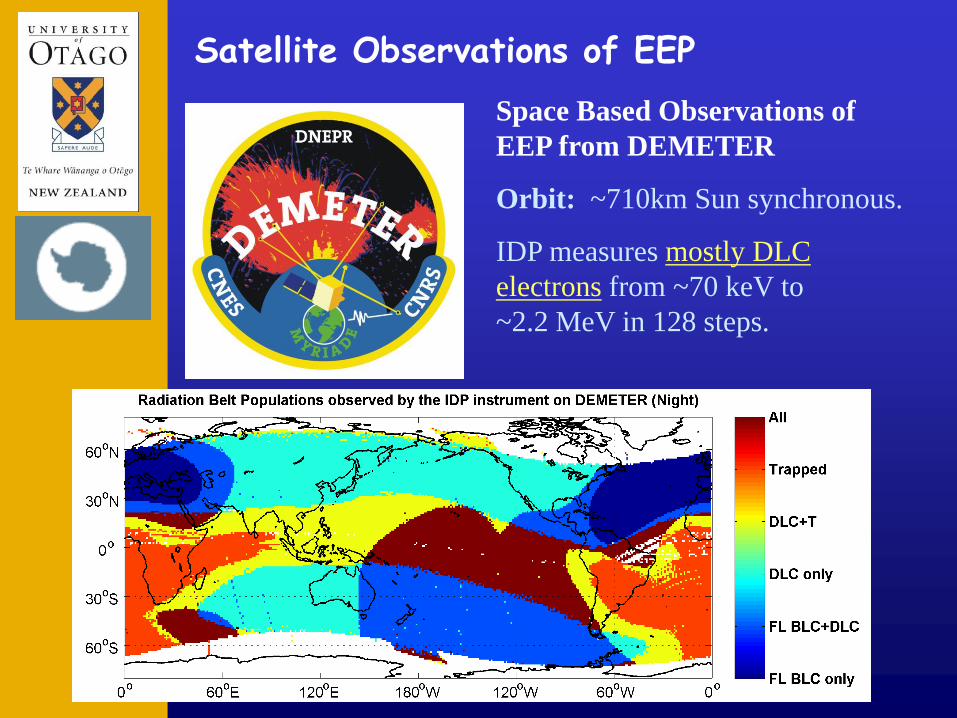
Satellite Observations of EEP
Space Based Observations of
EEP from DEMETER
Orbit: ~710km Sun synchronous.
IDP measures mostly DLC
electrons from ~70 keV to
~2.2 MeV in 128 steps.
Satellite Observations of EEP
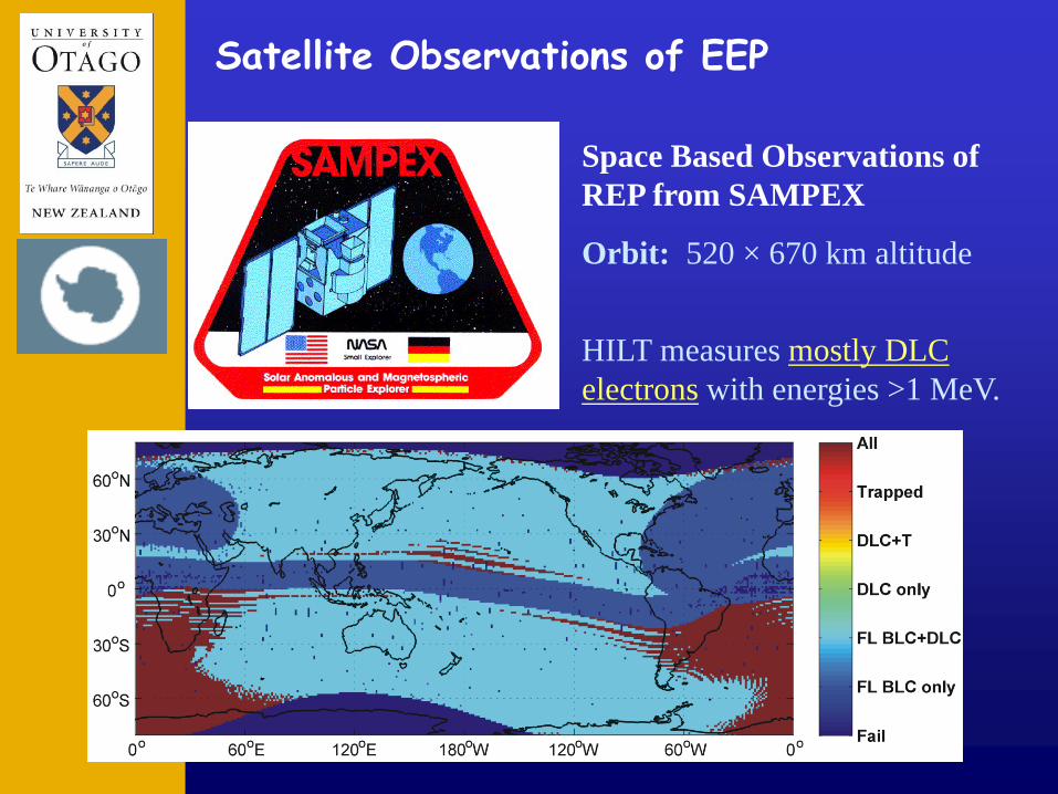
Space Based Observations of
REP from SAMPEX
Orbit: 520 × 670 km altitude
HILT measures mostly DLC
electrons with energies >1 MeV.
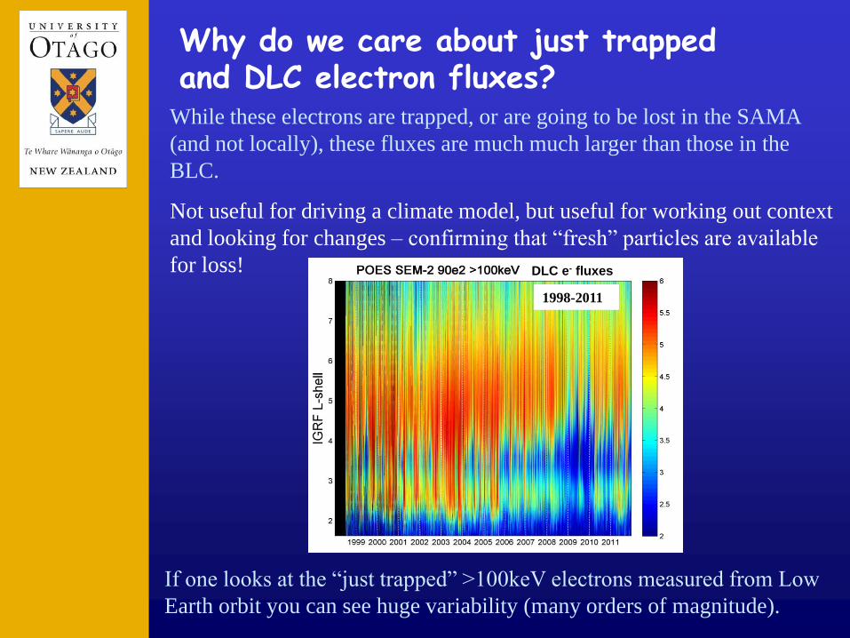
While these electrons are trapped, or are going to be lost in the SAMA
(and not locally), these fluxes are much much larger than those in the
BLC.
Not useful for driving a climate model, but useful for working out context
and looking for changes – confirming that “fresh” particles are available
for loss!
Why do we care about just trapped and DLC electron fluxes?
If one looks at the “just trapped” >100keV electrons measured from Low
Earth orbit you can see huge variability (many orders of magnitude).
DLC e- fluxes
1998-2011

Satellite Observations of EEP
Space Based Observations of EEP
from POES
Orbit: ~835 km Sun synchronous.
While suffering from numerous
limitations, POES is the most widely
used source of space based EEP
observations (and includes BLC) with
really long datasets available!
And MetOp-B
SEM-2 data to be
online from early
October!
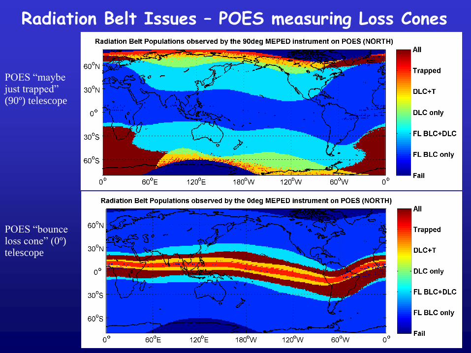
Radiation Belt Issues – POES measuring Loss Cones
POES “maybe just trapped” (90º) telescope
POES “bounce loss cone” (0º) telescope
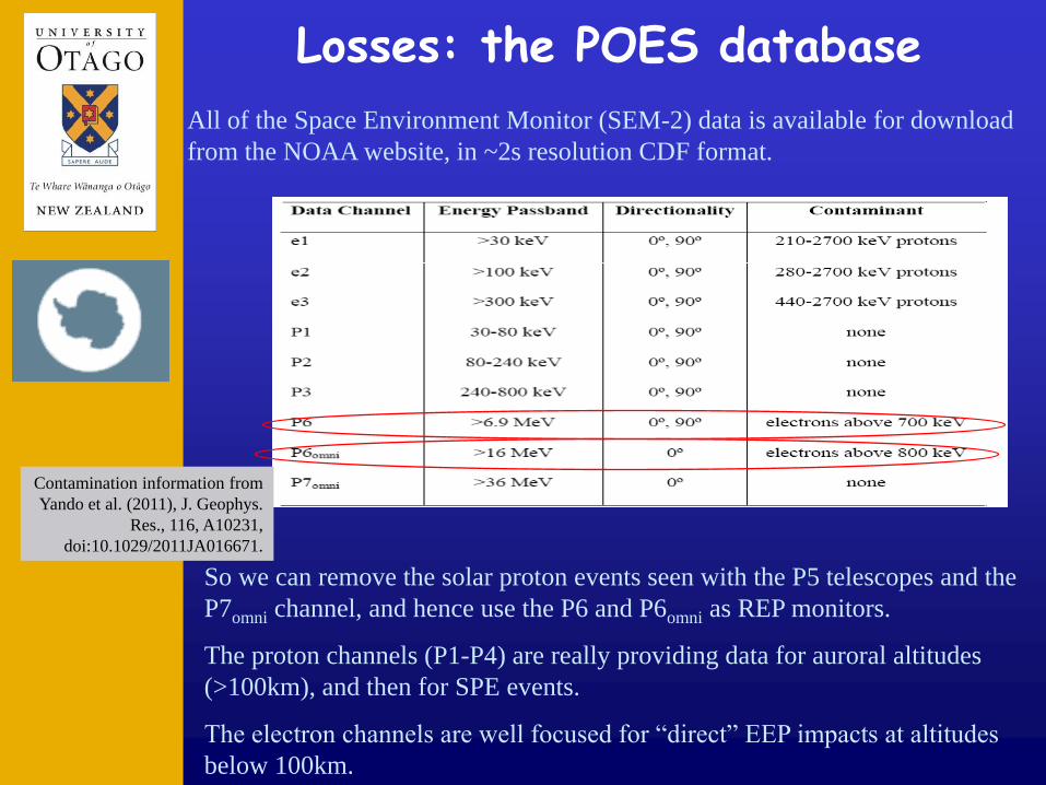
Losses: the POES database
All of the Space Environment Monitor (SEM-2) data is available for download
from the NOAA website, in ~2s resolution CDF format.
Contamination information from
Yando et al. (2011), J. Geophys.
Res., 116, A10231,
doi:10.1029/2011JA016671.
So we can remove the solar proton events seen with the P5 telescopes and the
P7omni channel, and hence use the P6 and P6omni as REP monitors.
The proton channels (P1-P4) are really providing data for auroral altitudes
(>100km), and then for SPE events.
The electron channels are well focused for “direct” EEP impacts at altitudes
below 100km.
The problems with POES SEM-2 e- data
The POES observations look perfect for our science needs. There is a lack of electron
precipitation data for energies >10 kev (that is altitudes below ~100 km), and the
POES SEM-2 does actually observe inside the Bounce Loss Cone. BUT we need to
beware as there are issues, caveats, and unknows to trip us up when we make use of
the electron observations.
Certainly, POES can be used to provide context and evidence that energetic electron
precipitation is happening (and probably relativistic electron precipitation too, if it is
intense enough as the response in P6 is pretty weak).
At least this point it is not really clear we can use the POES electron precipitation
data to feed global chemistry climate models to establish the significance of EEP.
There is a danger of “garbage in” = “garbage out” making the conclusions spurious.
Some basic issues.
1. The energy converge is poor (only >30, >100 & >300keV integral fluxes).
2. We can’t be certain what magnitude flux is actually going into the atmosphere.
3. The sensitivity of the instrument is pretty poor, so that “medium” levels of
>100keV and >300keV precipitation in quiet(ish) periods are normally lost/missed.
We are working on these issues, but its not as easy to fix or work-around as it
sounds!

Electron Instruments Lie when High Energy Protons Are Present
The last time we were in Boulder (HEPPA, 2009) Janet Green from
NOAA warned the POES users about the dangers of using the POES
SEM-2 electron measurements during solar proton events.
Some evidence – lets first look at a “quiet” situation (no SPE, no
strong EEP) as NOAA-15 crosses the north and south poles.

Electron Instruments Lie when High Energy Protons Are Present
The last time we were in Boulder (HEPPA 2009) Janet Green from
NOAA warned the POES users about the dangers of using the POES
SEM-2 electron measurements during solar proton events.
Some evidence – finally lets look at a “EEP” situation (no SPE,
active EEP) as NOAA-15 crosses the north and south poles.
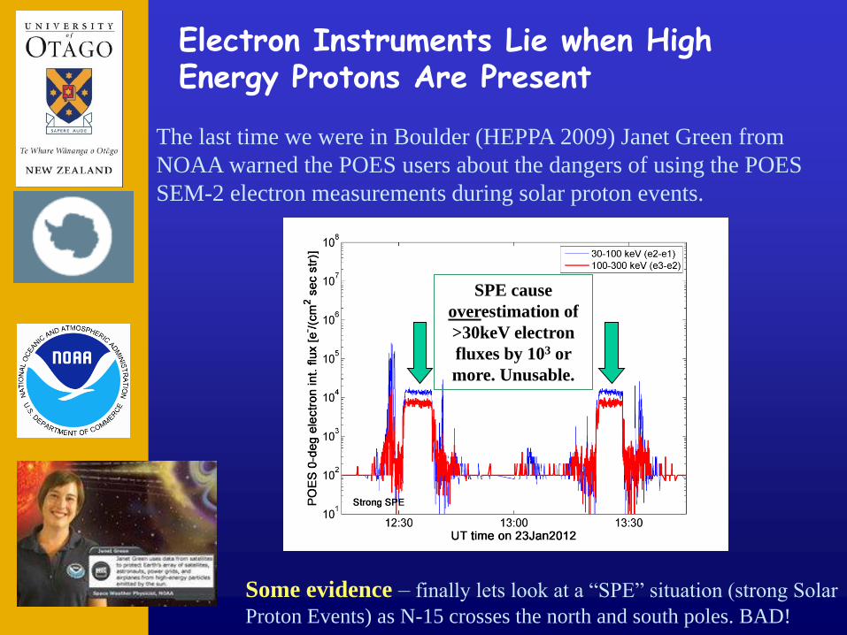
Electron Instruments Lie when High Energy Protons Are Present
The last time we were in Boulder (HEPPA 2009) Janet Green from
NOAA warned the POES users about the dangers of using the POES
SEM-2 electron measurements during solar proton events.
Some evidence – finally lets look at a “SPE” situation (strong Solar
Proton Events) as N-15 crosses the north and south poles. BAD!
SPE cause
overestimation of
>30keV electron
fluxes by 103 or
more. Unusable.
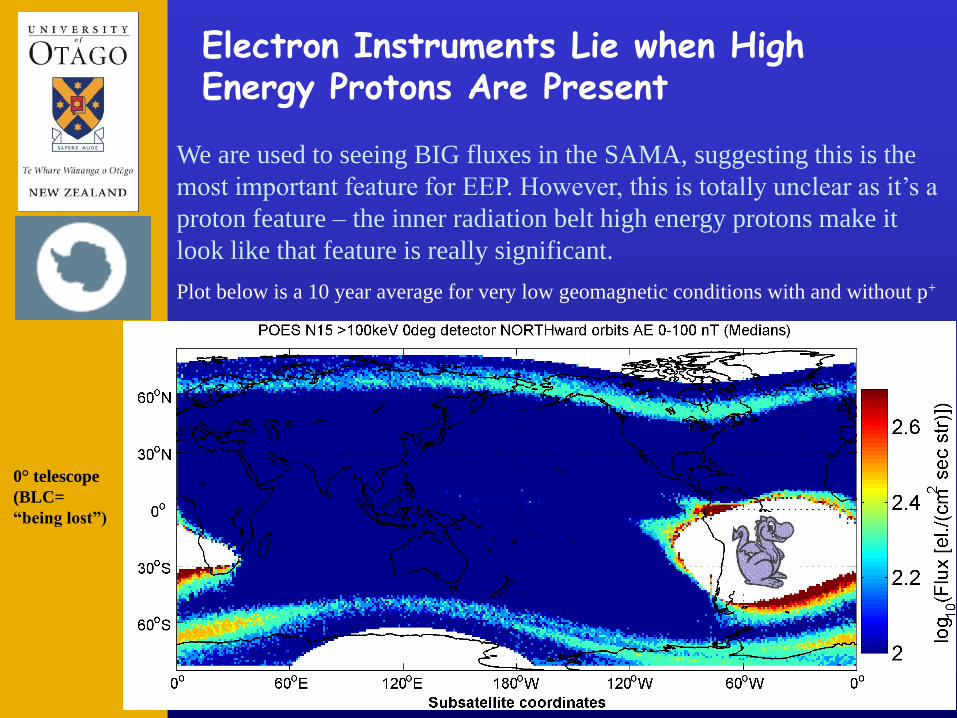
Electron Instruments Lie when High Energy Protons Are Present
We are used to seeing BIG fluxes in the SAMA, suggesting this is the
most important feature for EEP. However, this is totally unclear as it’s a
proton feature – the inner radiation belt high energy protons make it
look like that feature is really significant.
Plot below is a 10 year average for very low geomagnetic conditions with and without p+
0° telescope
(BLC=
“being lost”)
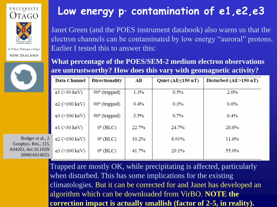
Low energy p+ contamination of e1,e2,e3
Janet Green (and the POES instrument databook) also warns us that the
electron channels can be contaminated by low energy “auroral” protons.
Earlier I tested this to answer this:
What percentage of the POES/SEM-2 medium electron observations
are untrustworthy? How does this vary with geomagnetic activity?
Trapped are mostly OK, while precipitating is affected, particularly
when disturbed. This has some implications for the existing
climatologies. But it can be corrected for and Janet has developed an
algorithm which can be downloaded from VirBO. NOTE the
correction impact is actually smallish (factor of 2-5, in reality).
Rodger et al., J.
Geophys. Res., 115,
A04202, doi:10.1029/
2008JA014023.
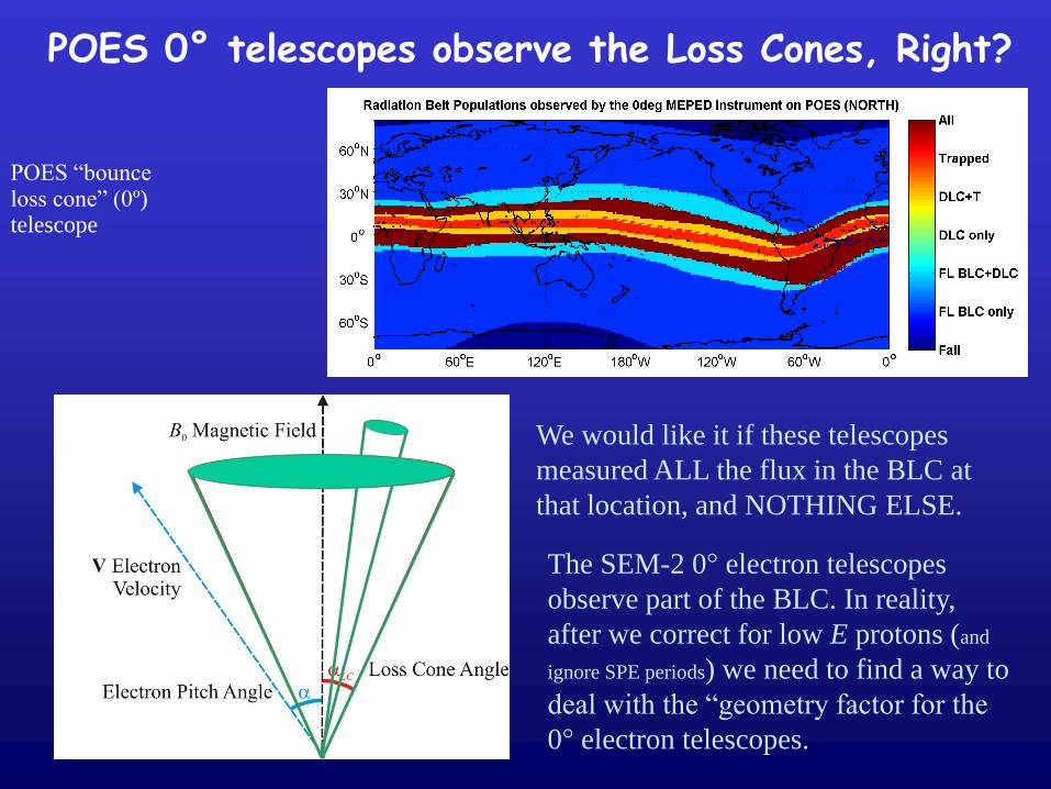
POES 0° telescopes observe the Loss Cones, Right?
POES “bounce loss cone” (0º) telescope
We would like it if these telescopes
measured ALL the flux in the BLC at
that location, and NOTHING ELSE.
The SEM-2 0° electron telescopes
observe part of the BLC. In reality,
after we correct for low E protons (and
ignore SPE periods) we need to find a way to
deal with the “geometry factor for the
0° electron telescopes.
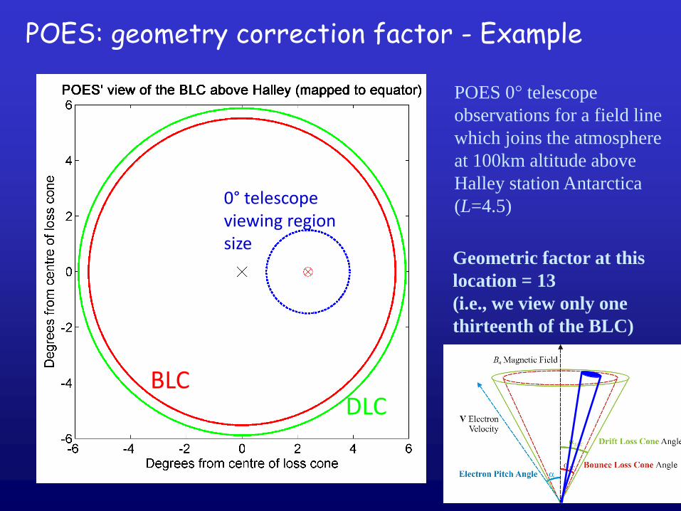
POES: geometry correction factor - Example
Geometric factor at this
location = 13
(i.e., we view only one
thirteenth of the BLC)
BLC DLC
0° telescope viewing region size
POES 0° telescope
observations for a field line
which joins the atmosphere
at 100km altitude above
Halley station Antarctica
(L=4.5)
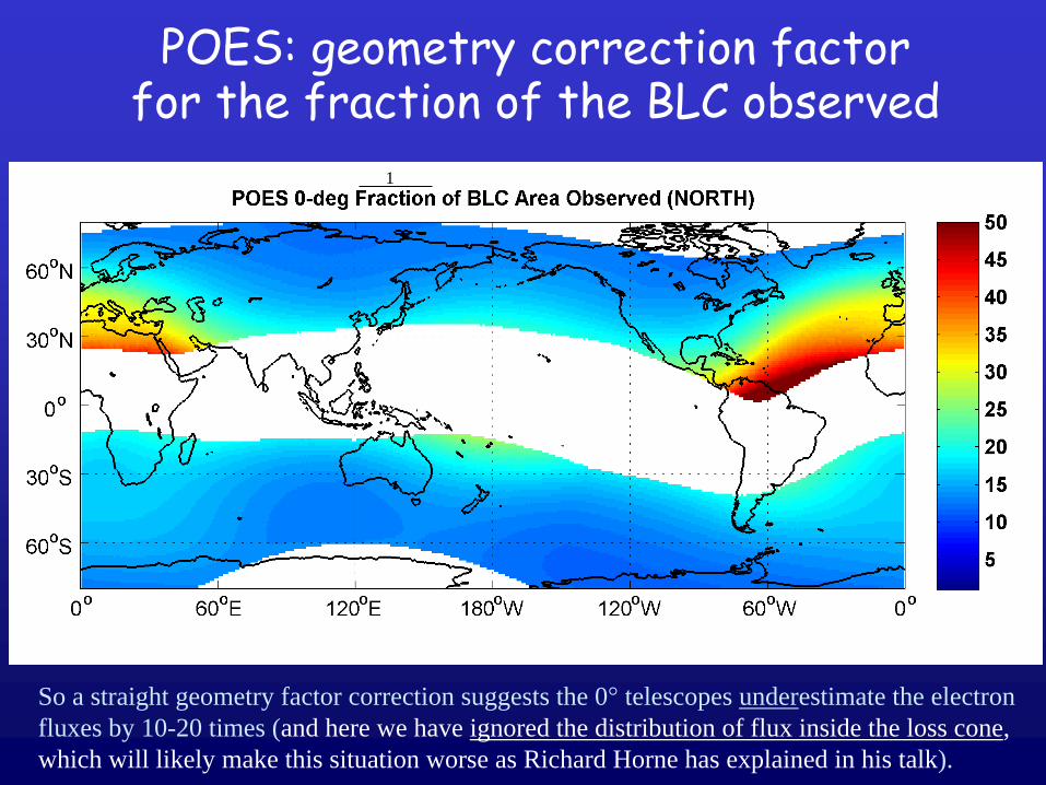
POES: geometry correction factor for the fraction of the BLC observed
1
So a straight geometry factor correction suggests the 0° telescopes underestimate the electron
fluxes by 10-20 times (and here we have ignored the distribution of flux inside the loss cone,
which will likely make this situation worse as Richard Horne has explained in his talk).

More information on this “geometry factor” in the poster by Mark Clilverd
Wednesday
afternoon poster
session (A2).
Here we look at
different events and
try and see if we can
find evidence of this
“geometry factor”
and related
corrections!

How to turn 3 integral electron fluxes into a reliable EEP flux?
From Yando et al. (2011), J.
Geophys. Res., 116, A10231,
doi:10.1029/2011JA016671.
From Clilverd et al.
(2012), J. Geophys.
Res., (in review),
doi:10.1029/2012JA01
8175.
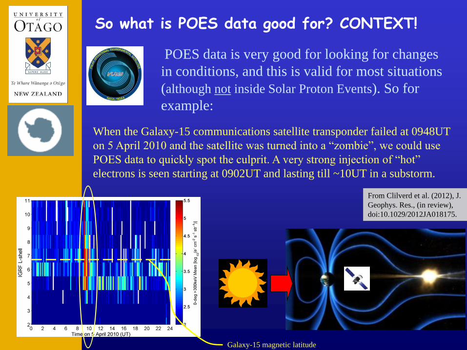
So what is POES data good for? CONTEXT!
POES data is very good for looking for changes
in conditions, and this is valid for most situations
(although not inside Solar Proton Events). So for
example:
When the Galaxy-15 communications satellite transponder failed at 0948UT
on 5 April 2010 and the satellite was turned into a “zombie”, we could use
POES data to quickly spot the culprit. A very strong injection of “hot”
electrons is seen starting at 0902UT and lasting till ~10UT in a substorm.
Galaxy-15 magnetic latitude
From Clilverd et al. (2012), J.
Geophys. Res., (in review),
doi:10.1029/2012JA018175.

Some extra facts! (no time to expand)
Energetic particle precipitation is not linearly linked to
geomagnetic indices, i.e. you can get lots of EEP with relatively
small geomagnetic disturbances.
Generally large geomagnetic disturbances will be linked to lots of
EEP and small disturbance levels will have smallish (but non
zero) precipitation magnitudes. BUTin addition we do see events
which are not strictly “geomagnetic storms” after which there are
really big precipitation levels.
From Hendry et al., AGU
Monograph "Dynamics of the
Earth's Radiation Belts and Inner
Magnetosphere", (in press),
doi:10.1029/2012BK001299, 2012.

We have been awarded a New Zealand
Marsden Funded project to investigate this
very issue:
“Evaluating the Impact of Excess Ionization
on the Atmosphere (EI EI A)”
My main support comes from:
Significant support, including for
my PostDoc Ian Whittaker who is
working on POES spectral fitting,
has been provided by the EU FP7
PLASMON project.
And I better not forget
Conclusions • Energetic electron precipitation (EEP) appears to be a significant part of the
variability of the mesosphere (i.e. “directly” significant).
• Observations of EEP from low-Earth orbiting satellites provide context for the
variation in the EEP levels: - either through observations of the “only just trapped” population
- or by trying to make measurements of the bounce loss cone
• While there is experimental evidence that relativistic electron precipitation is
important in the atmosphere, we struggle to measure it atall (lack of data).
• One of the best sources we have for this purpose are from the Polar
Operational Environmental Satellites (POES) .
BUT THESE DATA HAVE ISSUES.
• SPE cause overestimation of >30 keV electron fluxes by 103 or more. At these
times, or in the SAMA, the observations are almost certainly totally unusable.
• Low energy protons also affect the electron precipitation observations. But
there is an algorithm to correct for this as the effect is smallish (typically less
than a factor of 2).
• The geometry factor AND the energy fitting issue are still open questions and
are being worked on – they could easily lead to changes more than a factor of
10 (probably an underestimation of the EEP).
Craig standing in front of the Space Shuttle Discovery (OV-103) in the space hall of the Udvar Hazy Center (Smithsonian Air and Space Museum). He was visiting the Museum on the way to the VERSIM workshop in Brazil, and we had to spend most of a day around Dulles airport [31 August 2012].
Are there any questions?
Thankyou!