Policy Research Working Paper 5055

Endowment Structures, Industrial Dynamics, and Economic Growth

Jiandong Ju Justin Yifu Lin

Yong Wang

The World BankDevelopment Economics Vice PresidencySeptember 2009

WPS5055P

ublic

Dis

clos

ure

Aut

horiz

edP

ublic

Dis

clos

ure

Aut

horiz

edP

ublic

Dis

clos

ure

Aut

horiz

edP

ublic

Dis

clos

ure

Aut

horiz

edP

ublic

Dis

clos

ure

Aut

horiz

edP

ublic

Dis

clos

ure

Aut

horiz

edP

ublic

Dis

clos

ure

Aut

horiz

edP

ublic

Dis

clos

ure

Aut

horiz

ed

Produced by the Research Support Team

Abstract

The Policy Research Working Paper Series disseminates the findings of work in progress to encourage the exchange of ideas about development issues. An objective of the series is to get the findings out quickly, even if the presentations are less than fully polished. The papers carry the names of the authors and should be cited accordingly. The findings, interpretations, and conclusions expressed in this paper are entirely those of the authors. They do not necessarily represent the views of the International Bank for Reconstruction and Development/World Bank and its affiliated organizations, or those of the Executive Directors of the World Bank or the governments they represent.

Policy Research Working Paper 5055

This paper develops a dynamic general equilibrium model to explore industrial evolution and economic growth in a closed developing economy. The authors show that industries will endogenously upgrade toward the more capital-intensive ones as the capital endowment becomes more abundant. The model features a continuous inverse-V-shaped pattern of industrial evolution driven by capital accumulation: As the capital endowment reaches a certain

This paper—a product of the Development Economics Vice Presidency—is part of a larger effort in the World Bank to contribute to a better understanding of the economic and social development process. Policy Research Working Papers are also posted on the Web at http://econ.worldbank.org. The author may be contacted at research@worldbank.org.

threshold, a new industry appears, prospers, then declines and finally disappears. While the industry is declining, a more capital-intensive industry appears and booms, ad infinitum. Explicit solutions are obtained to fully characterize the whole dynamics of perpetual structural change and economic growth. Implications for industrial policies are discussed.

Endowment Structure, Industrial Dynamics, andEconomic Growth

Jiandong Ju�, Justin Yifu Liny, Yong Wangz�

This version: October 20, 2009

Abstract

This paper develops a dynamic general equilibrium model to explore industrialevolution and economic growth in a closed developing economy. The authorsshow that industries will endogenously upgrade toward the more capital-intensiveones as the capital endowment becomes more abundant. The model featuresa continuous inverse-V-shaped pattern of industrial evolution driven by capitalaccumulation: As the capital endowment reaches a certain threshold, a newindustry appears, prospers, then declines and �nally disappears. While theindustry is declining, a more capital-intensive industry appears and booms,ad in�nitum. Explicit solutions are obtained to fully characterize the wholedynamics of perpetual structural change and economic growth. Implicationsfor industrial policies are discussed.KeyWords: Endowment, Industrial Dynamics, Economic Growth, Structural

ChangeJEL Codes: L50, O14, O40

�University of Oklahoma, Email address: jdju@ou.edu; yWorld Bank, Email address:justinlin@worldbank.org; zHong Kong University of Science and Technology, Email address:yongwang@ust.hk. For detailed comments and helpful discussions, we would like to thank PhilippeAghion, Jinhui Bai, Gary Becker, Veronica Guerrieri, Chang-Tai Hsieh, Aart Kraay, Kala Krishna,Norman Loayza, Francis T. Lui, Erzo Luttmer, Rachel Ngai, Paul Romer, Harald Uhlig, DanyangXie, as well as many other seminar participants in several institutions. Ju and Wang thank theWorld Bank for the hospitality and �nancial support. All remaining errors are our own.

0

"The growth of GDP may be measured up in the macroeconomic treetops, but

all the action is in the microeconomic undergrowth, where new limbs sprout, and

dead wood is cleared away."

�World Bank Commission on Growth and Development (2008, pp.2-3)

1 Introduction

The main goal of this paper is to develop a formal model to explain the industrial

dynamics along the path of economic growth in developing countries. We show how

the optimal leading industries are structurally di¤erent at di¤erent development

stages, depending mainly on the economy�s endowment structure and its evolution.

Sustained economic development from a low-income status to high-income status in

countries in modern times is characterized by continuous technological innovation

and industrial upgrading (see Chenery (1960), Kuznets (1966), Maddison (1980),

Chenery, Robinson, and Syrquin (1986), Hayami and Godo (2005)). Beneath the

GDP growth, the products or major industries in the manufacturing sector of these

economies are continuously changing over time. First labor-intensive goods such

as textiles and shoes are produced, then those industries decline and are gradually

replaced by the more capital-intensive industries such as machinery and electronics,

which also decline later while even more capital-intensive industries arise such as

cars and aircraft, and so forth. Such a pattern, as shown in Figure 1, was referred as

the �ying geese pattern of economic development by Akamatsu (1962) in the 1930s

and further developed by Kojima (2000).

1

Figure 1: Japan�s Industrial Upgrading and Product Evolution (Kojima, 2000)

Surprisingly, however, this continuous waxing and waning pattern of industrial

development has rarely been formalized in the growth and development literature,

although it has been well documented for a long time.1 Recall that most of the

earlier growth models aim to match the Kaldor facts and typically assume the same

aggregate production function for countries at di¤erent development stages, which

naturally leads economists to focus on the cross-country di¤erences in productivity

or human capital while ignoring the structural di¤erences in the industries for

countries at di¤erent development stages (see Kaldor (1961), Solow (1965), Barro

and Sala-i-Martin (2004)).2 Recent growth models do start to address various

types of structural change. Most of them mainly explore the long-run trend shift

in the compositions of aggregate agriculture, industry, and service sectors without

exploring the dynamics within the aggregate sectors, such as the continuous upgrading

of manufacturing industries. Consequently, they do not characterize the inverse-V-shaped

industrial dynamics described above. For example, Lucas (2004) studies the rural-urban

1There are some exceptions: Vernon (1965) develops a product-cycle argument to explain howthe location of production for a commodity might shift across countries over time. Schumpeter(1942) expatiates the idea of creative destruction based on technology advancement instead ofcapital endowment improvement, which is further developed by Aghion and Howitt (1992). Thosestudies focused mainly on the R&D-driven mechanism of industrial evolution in developed countriesinstead of developing countries.

2Kaldor facts refer to the relative constancy of the growth rate of total output, the capital-outputratio, the real interest rate, and the share of labor income in GDP.

2

transformation driven by the externality of human capital. Buera and Kaboski

(2009) focus on the expansion of the service sector. Some other works strive to

match Kuznets facts, which state that development is typically a process of a

decline in agriculture, a rise in services, and a hump-shaped change in industry.

In addition, that literature mainly focuses on the long-run (balanced or asymptotic)

growth rate (or steady state) without explicitly and completely characterizing the

whole dynamics for the structural change per se. Moreover, in those models the

structural changes are driven either by the demand shift in the consumption goods

as people get richer (see Laitner (2000), Caselli and Coleman (2001), Kongsamut,

Rebelo, and Xie (2001), Gollin, Parente, and Rogerson (2002)), or by the di¤erent

productivity growth across di¤erent sectors as �rst suggested by Baumol (1967),

and further developed by Hansen and Prescott (2002) and Ngai and Pissarides

(2007). In this paper, we argue that the inverse-V-shaped industrial dynamics in

a developing country is driven mainly by the change in its endowment structure.

The endowments are given at any given time and changeable over time. One of

the key di¤erences between a developed and developing country is the di¤erence

in the relative abundance of capital in their endowment structures. The economic

development process in a developing country is characterized by the continuous

upgrading of its endowment structure from relatively scarce in capital and relatively

abundant in labor or natural resources to relatively abundant in capital and relative

scarce in labor/natural resources. Lin (2003, 2009) argues that the optimal industrial

structure in an economy at a given time should be consistent with the given endowment

structure at that time: as capital accumulates and becomes relatively cheaper, the

industries should optimally upgrade toward more capital-intensive ones accordingly.

Motivated by Lin�s argument, our model will show that the driving force for the

�ying-geese pattern of industrial upgrading in the development process of a developing

country is the continuous capital deepening in the endowment structure.

Acemoglu and Guerrieri (2008) have examined how the capital deepening has an

3

asymmetric impact on the sectors with di¤erent capital intensities, but their main

objective is to study how the elasticity of substitution between two sectors with

di¤erent capital shares a¤ects the long-run asymptotic aggregate growth rate. Moreover,

their model has two sectors and is thus unable to explain the �ying-geese pattern of

repetitive inverse-V-shaped industrial upgrading dynamics.

It is very important to understand the widely observed inverse-V-shaped industrial

dynamics in the process of economic development. What type of industry should

we expect to dominate at a certain stage of development? Would it be optimal

for the government in a low-income country to support the development of certain

industries that prevail in high-income countries? To answer these questions, it is

not enough to merely recognize the long-run structural change among the primary,

secondary, and tertiary sectors or in the rural-urban transformation.

In what follows, we develop a growth model featuring this inverse-V-shaped industrial

dynamics along the development path. The major force driving the structural

change is the increase in the capital-labor ratio (or alternatively, endowment structure).

As capital becomes more abundant and relatively cheaper, the more capital-intensive

industrial goods are produced, because the more capital-intensive industry products

are not only more a¤ordable but also more desirable for the consumers. At the same

time, the more labor-intensive goods are gradually displaced. As capital becomes

even more abundant, goods with an even higher capital intensity become more

desirable to produce and consume. This generates the endless inverse-V-shaped

industrial dynamics. Our model underscores the key role played by the changes in

endowment structure rather than productivity increase. This might be reasonable

because our model is mainly geared toward developing economies where industrial

upgrading relies mainly on borrowing existing technologies from developed countries

(Hayami and Goto (2005)), in contrast to the developed economies where huge

research and development expenditure is required for technology innovation and

industrial upgrading.

4

To highlight the industrial dynamics, we deviate from the standard practice in the

growth literature, which typically only focuses on the steady state or the long-run

(balanced or asymptotic) growth rate. Instead, we obtain the explicit solution for

the whole dynamics in the structural changes, even though we are considering a

dynamic economy with an in�nitely dimensional commodity space and an in�nite

time horizon.3 We decompose this seemingly complicated structural analysis into

two steps. First, along the time dimension, the representative household simply

decides the allocation of capital for producing consumption goods and savings. The

household�s capital allocation determines the evolution of capital endowment and the

intertemporal use of capital in production. Then, along the cross-section dimension,

the capital allocated for production determines the production structures (industrial

choices) as if it were a static model. Ultimately, the mathematical problem is

reduced to dynamic optimization with switching state equations. This approach,

which we call a dynamic structural analysis, can tremendously simplify the analysis

of perpetual industrial upgrading with long-run growth.

Our paper is related to the literature of quality-ladder growth models because in

our model di¤erent industrial goods are modelled as perfect substitutes and are

produced with di¤erent technologies. Aghion and Howitt (1992) emphasize that

the �rm�s incentives to earn monopolistic rents justify its endeavor to undertake

risky and costly R&D, which ultimately causes the creative destruction (also see

Grossman and Helpman, 1991a). Our model is methodologically closest in spirit to

Stokey (1988), who characterizes how the learning-by-doing keeps the band of the

produced commodities moving toward higher and higher qualities. The main goals of

that literature, however, are to generate sustained economic growth at the aggregate

level instead of trying to explain the inverse-V-shaped industrial dynamics. More

3There may be a technical reason why the well-recognized fact of industrial dynamics hasrarely been formalized in growth models. Closed-form solutions for transitional dynamics aretypically very hard to obtain even in most of the two-sector growth models, but the aforementionedinverse-V-shaped industrial dynamics is by nature the transitional dynamics per se, so the industrialupgrading with an in�nite-dimensional commodity space appears even more unwieldy.

5

importantly, all these papers try to emphasize the role of technological advancement

or knowledge accumulation with stable industries while our paper stresses the role

of capital accumulation and industrial upgrading. In addition, this literature, like

other growth models, also mainly studies the long-run balanced growth path while

leaving the transitional dynamics aside. The industrial climbing result in Stokey

(1988), for example, is obtained essentially through comparative statics rather than

the full-blown dynamic model. By contrast, we are able to provide the closed-form

solutions for all the dynamics.

Simple comparative statics in our static model shows how the change in the endowment

structure determines the changes in industrial structures, a result similar to the

Heckscher-Ohlin model with multiple diversi�cation cones (see Leamer (1987), Schotter

(2003)). However, there is a nontrivial di¤erence. These multiple diversi�cation

cone models mainly consider open economies where the production structure of a

country is determined by international specialization. By contrast, in our closed

economy model, the households and �rms select endogenously which set of products

to consume and produce. More importantly, our dynamic model enables us to

obtain explicit solutions to characterize the whole inverse-V-shaped dynamics of

the in�nite industrial upgrading, while H-O models with multiple diversi�cation

cones are mostly static. To highlight the direct impact of endowment change on the

industrial dynamics, we purposefully ignore the e¤ect of international specialization

according to comparative advantage and only consider a closed economy in this

paper.4 We suspect that our main proposition, namely, the change in endowment

structures drives the change in industrial structures, will be only strengthened

4Notice that in our paper a developing country is implicitly assumed to be able to freely borrowthe technology knowhow of more capital intensive industries from the developed countries. Themain conclusions of the model are expected to hold in an open economy model. Moreover, exceptin an extremely small economy, the domestic market plays a major role in economic development.For example, Chenery, Robinson, and Syrquin (1986) �nd that expansion in the domestic demandaccounted for a 72%-74% increase in domestic industrial output in those countries with populationlarger than 20 million, and that even for small and manufacturing-oriented countries with populationless than 20 million, domestic demand expansion accounts for a 50%-60% increase in the totalindustrial output. See Murphy, Shleifer and Vishy (1989) for more argument.

6

in an open economy, as predicted by standard H-O trade models.5 Our model

characterizes the �rst-best scenario in which the industrial structures evolve optimally

in a perfectly competitive and frictionless economy. In such an ideal world, no

government intervenes and the market itself can identify and support the right

industries at each development stage. But what if the government pursues a wrong

development strategy and pushes the economy to develop some inappropriate industries?

We show in this paper that such policy mistakes may sometimes cause the economy

to fall into a poverty trap such that long-run growth becomes impossible without

foreign help. The markets are far from perfect in the real world, so it may be

desirable for the government to have an industrial policy which will help to provide

�rms with information, coordinate �rms�investments and compensate for externalities

produced by pioneer �rms (Murphy, Shleifer, and Vishny (1989), Lin (2009)). However,

the prerequisite for a successful industrial policy is to identify what type of industries

should be supported at each di¤erent development stage. Our �rst-best characterization

sets a theoretical benchmark that may potentially help us think further about these

issues.

The paper is organized as follows: Section 2 presents the static model. The dynamic

model is analyzed in Sections 3 and 4. Welfare consequences of the mistakes in

industrial choices are discussed in Section 5. Section 6 concludes. Technical proofs

and derivations are put in the Appendix.

2 Static Model

2.1 Setup

Consider a closed developing economy with a unit mass of identical households.

Each household is endowed with L units of labor and E units of capital, which

5Ventura (1997) shows theoretically how factor-price-equalization driven by international tradecan explain the rapid catching-up growths of several export-oriented East Asian economies.Krugman (1979) constructs a North-South trade model to explore how the catching up processdepends on whether the rich country�s innovation speed exceeds the poor country�s imitation speed.

7

conceptually consists of both tangible physical capital and intangible capital. For

parsimony purpose, we will narrowly interpret this "composite capital" as physical

capital from now on in this qualitative investigation. The given commodity space

has in�nite dimensions. Let cn denote the consumption of good n = 0; 1; 2; ::. In

particular, good 0 may be interpreted as a household product, and good n for n � 1

may be interpreted as �industrial�product. De�ne the aggregate good as

C =

1Xn=0

�ncn;

where the quality coe¢ cient for good i is �n.6 We require cn � 0 for any n: The

representative household�s utility function is CRRA:

U =C1�� � 11� � ; where � 2 (0; 1]: (1)

All the production technologies exhibit constant returns to scale. In particular,

good 0 is produced with labor only. One unit of labor produces one unit of good 0.

For any industrial good n = 1; 2; 3; :::; both labor and capital are required and the

production functions are Leontief: 7

Fn(k; l) = minfk

an; lg; (2)

6This assumption is quite standard in the vertical innovation growth literature. Thespeci�cation is also mathematically isomorphic to the following alternative economic interpretation:C is the �nal good while all the cn; n = 0; 1; 2; ::: are intermediate goods, so �n should beinterpreted as the "productivity" for good n. It is not unusual in growth literature to assume perfectsubstitutability for the output across di¤erent production activities. For example, the agricuturalMalthus production and the modern Solow production are two linearly additive components for thetotal output in Hansen and Prescott (2002) and Lucas (2009). A further discussion will be devotedto this "perfect substitutability" assumption later.

7This assumption drastically simpli�es the dynamic strucutral analysis partly by giving us alot of linearities. In the Appendix, we show that the main results remain valid with Cobb-Douglassfunction, but the dynamic analysis will be much more complex. Houthakker (1956) shows thatLeontief production functions with Pareto-distribution heterogenous paratermers can aggregateinto Cobb-Douglass production functions. Lagos (2006) constructs another distribution that canaggregate heterogenous Leontief functions into CES production functions. These may be helpful inunderstanding how �rm heterogeneities may a¤ect our results, which is a very interesting researchdirection.

8

where an is the capital intensity of producing one unit of good n: All the markets

are perfectly competitive. Let pn denote the price of good n. Let r denote the rental

price of capital and w denote the wage rate. Thus, �rm�s zero pro�t function implies

that p0 = w and pn = w + anr for n = 1; 2; 3; ::.

We assume

�n = �n; an = an (3)

� > 1; a > 1, and a� 1 > �: (4)

Therefore, a higher-index good has a higher quality but is more capital intensive.

The last inequality in (4) not only rules out the trivial case that only the highest

quality good is produced in any equilibrium, but also simpli�es our analysis, as will

be clear shortly.

The household problem is to maximize (1) subject to the following budget

constraint1Xn=0

pncn = wL+ rE (5)

Set up the Lagrangian with the multiplier denoted by �, and we obtain the following

optimality condition for consumptions:

�n

1Xn=1

�ncn + c0

!��� �pn; for 8n � 0; (6)

�= �when cn > 0:

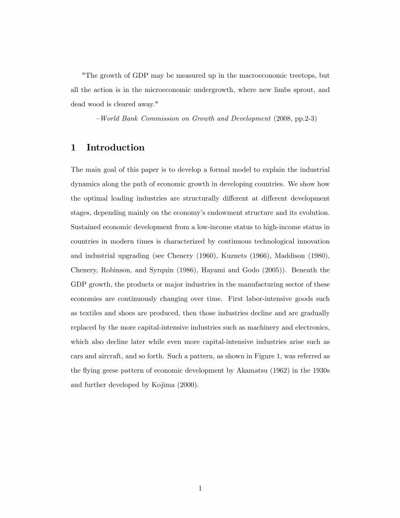
2.2 Market Equilibrium

The market equilibrium is determined by the endowment structure (capital per

capita), EL : In the Appendix, we show that at most two goods are produced simultaneously

in the equilibrium and that these two goods have to be adjacent in capital intensities.

The intuition is the following: Suppose goods n and n + 1 are produced for some

9

n � 1. From consumer�s maximization problem, we immediately have

MRSn+1;n = � =pn+1pn

=w + an+1r

w + anr;

which implies thatr

w=

�� 1an(a� �) : (7)

Obviously,MRSj;j+1 >pjpj+1

whenever rw >��1

aj(a��) ; andMRSj;j�1 >pjpj�1

whenever

rw <

��1aj�1(a��) for any j = 1; 2; ::. Therefore, when

rw =

��1an(a��) , good n+1 must be

strictly preferred to good n+ 2; because the marginal rate of substitution is larger

than their relative price. This means that cj = 0 for all j � n+ 2. Using the same

logic, we can also verify that cj = 0 for all 1 � j � n� 1. In addition, condition (4)

ensures that good 0 will not be produced, as can be veri�ed by simply comparing

the marginal rate of substitution between good n and good 0 and their price ratio.

Similarly, when goods 0 and 1 are produced, we can show that good 1 is strictly

preferred to any good n � 2:

The market clearing conditions for labor and capital are

cn + cn+1 = L (8)

cnan + cn+1a

n+1 = E: (9)

10

E

L0

B

A

W

1+na

'A

'B

na

'W

1−na

Figure 2. How Endowment Stucture Determines Optimal Industries

The market equilibrium can be illustrated graphically in Figure 2, where labor

and capital are represented by horizontal and vertical axes, respectively. O represents

the origin for the country. Lines Oan = (1; an) cn and Oan+1 =�1; an+1

�cn+1

are the vectors of factors used in producing cn and cn+1 in the equilibrium. Let

point W = (L;E) be the factor endowment of the country. If W = anL; only

good n is produced. Similarly, if W = an+1L; only good n + 1 is produced. When

anL < W < an+1L; both goods n and n+1 are produced. The factor market clearing

conditions, (8) and (9), determine the usages of labor and capital in industries n

and n+1; which are represented by vector OA and vector OB in the parallelogram

OAWB, respectively. If the capital endowment increases from W to W 0; the new

equilibrium becomes parallelogramOA0W 0B0 so that cn decreases but cn+1 increases.

More precisely, the equilibrium output of each commodity cn, the relative factor

prices rw ; and the corresponding aggregate output C are summarized in the following

table.

11

Table 1: Static Equilibrium

0 � E � aL anL � E < an+1L for n � 1

c0 = L� Ea cn =

Lan+1�Ean+1�an

c1 =Ea cn+1 =

E�anLan+1�an

cj = 0 for 8j 6= 0; 1 cj = 0 for 8j 6= n; n+ 1rw =

��1a

rw =

��1an(a��)

C = L+ (�� 1)Ea C = �n+1��nan+1�anE +

�n(a��)a�1 L

, E0;1 =a��1(C � L) , En;n+1 =

hC � �n(a��)

a�1 Lian+1�an�n+1��n

The whole static equilibrium is summarized verbally in the following proposition.

Proposition 1 In a closed economy, the static market equilibrium is determined

by the endowment structure, EL : Generically, only two goods adjacent in capital

intensities are produced in equilibrium. As capital per capita increases, every commodity

exhibits an inverse-V-shaped life cycle. A good enters the market, prospers (its

output increases) and then declines, and �nally is fully replaced by another product

with a higher capital intensity. The ratio of the interest rate to the wage rate declines

as EL increases.

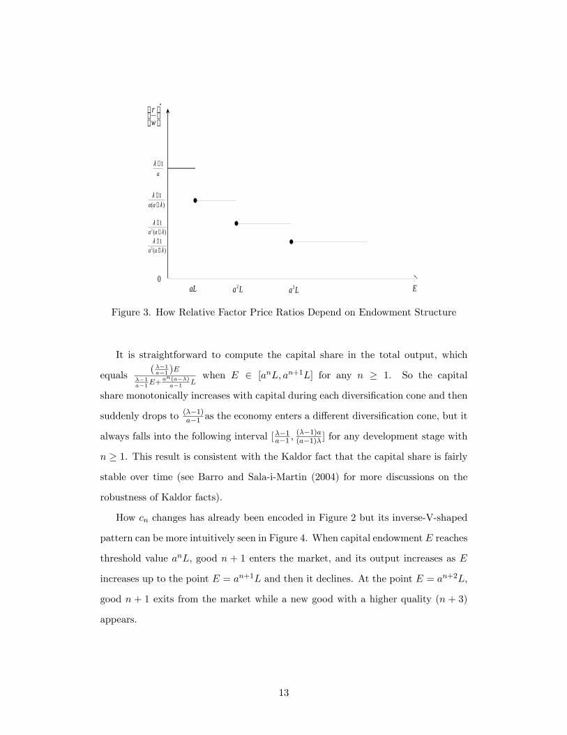
Figure 3 shows that the relative factor prices rw , which declines in a stair- shaped

fashion as E increases. This discontinuity results from the Leontief production

assumption but the �at part is more general: During the structural change, resource

reallocation occurs without changes in relative prices.

12

*

wr

EaL La2 La3

a1−λ

0

)(1λ

λ−−

aa

)(1

2 λλ

−−

aa

)(1

3 λλ

−−

aa

Figure 3. How Relative Factor Price Ratios Depend on Endowment Structure

It is straightforward to compute the capital share in the total output, which

equals(��1a�1 )E

��1a�1E+

an(a��)a�1 L

when E 2 [anL; an+1L] for any n � 1. So the capital

share monotonically increases with capital during each diversi�cation cone and then

suddenly drops to (��1)a�1 as the economy enters a di¤erent diversi�cation cone, but it

always falls into the following interval [��1a�1 ;(��1)a(a�1)� ] for any development stage with

n � 1. This result is consistent with the Kaldor fact that the capital share is fairly

stable over time (see Barro and Sala-i-Martin (2004) for more discussions on the

robustness of Kaldor facts).

How cn changes has already been encoded in Figure 2 but its inverse-V-shaped

pattern can be more intuitively seen in Figure 4. When capital endowment E reaches

threshold value anL; good n + 1 enters the market, and its output increases as E

increases up to the point E = an+1L and then it declines. At the point E = an+2L;

good n + 1 exits from the market while a new good with a higher quality (n + 3)

appears.

13

*nc

EaL La2 La30

L

La4

:*0c :*

1c :*2c :*

3c

Figure 4. How Each Industry Depends on the Endowment

The above equilibrium in our closed economy model turns out to be very similar

to the H-O trade model with multiple diversi�cation cones. However, the main

mechanisms are totally di¤erent. Leamer (1987) and other papers in this literature

mainly consider (small) open economies where the production structure of a country

is determined by international specialization and each good has to be consumed.

In our closed-economy general equilibrium model, which set of goods should be

consumed and produced is an endogenous decision, depending solely on the domestic

demand and endogenous relative factor prices, which are mainly dictated by the

endowment structure.

3 Dynamic Model

In this section, we will develop a dynamic model to capture the complete industrial

dynamics along the path of economic growth. The key idea is to break down the

evolution analysis of production structures into two steps. Along the time dimension,

the representative consumer decides her intertemporal consumption �ows of the

aggregate good C and makes the saving and investment decisions. This dynamic

decision determines the evolution of endowment structure KL and the optimal capital

14

expenditure EL at every time point t: In the cross section dimension, the capital

expenditure EL then determines the production structures, exactly the same as in

the static model.

By the second Welfare Theorem, we can characterize the competitive equilibrium

by resorting to the following social planner problem:

maxC(t)

Z 1

0

C(t)1�� � 11� � e��tdt

subject to

�K = �K(t)� E(C(t)) (10)

K0 is given:

where � is the time discount rate. K(t) is the amount of working capital at t. At

each time, the old capital can be transformed into new working capital using the

standard AK model technology and � is the exogenous technology parameter net of

the depreciation rate. All the new working capital can be used to either produce the

consumption good or to save/invest. E(C(t)) is the total capital used to produce

the aggregate consumption C(t). All the consumption goods are non-storable. The

total labor endowment L is constant over time.8 To ensure positive consumption

growth, we assume � � � > 0. To exclude the explosive solution, we also assume

���� (1� �) < �. Putting them together, we assume

0 < � � � < ��: (11)

From Table 1, we know that E(C) is a strictly increasing, continuous, piece-wise

linear function of C. It is not di¤erentiable at C = �iL, for any i = 0; 1; :::.

Therefore, the above dynamic problem may involve changes in the functional forms

8 It is straightforward to examine how exogenous changes in the �e¤ective labor�(for example,let L(t) = L0e t for some > 0) may a¤ect economic dynamics.

15

of the state equation: (10) can be explicitly rewritten as

�K =

8>>>><>>>>:�K; when C � L

�K � E0;1(C); when L � C � �L

�K � En;n+1(C); when �nL � C � �n+1L; for n � 1

;

where En;n+1(C) is de�ned in Table 1 for any n � 0. We can easily verify that,

in this dynamic optimization problem, the objective function is strictly increasing,

di¤erentiable and strictly concave while the constraint set forms a continuous convex-valued

correspondence, hence the equilibrium must exist and also be unique.

Let t0 denote the last time point when the aggregate consumption equals L; and

tn denote the �rst time point when C = �nL for n � 1: As can be shown later, the

aggregate consumption C is monotonically increasing over time in the equilibrium,

hence the problem can be also written as

maxC(t)

Z t0

0

C(t)1�� � 11� � e��tdt+

1Xn=0

Z tn+1

tn

C(t)1�� � 11� � e��tdt

subject to

�K =

8>>>><>>>>:�K when 0 � t � t0

�K � E0;1(C); when t0 � t � t1

�K � En;n+1(C); when tn � t � tn+1; for n � 1

;

K0 is given:

According to Table 1, in time period t0 � t � t1; goods 0 and 1 are produced

and E(C) � E0;1(C) = a��1(C � L), while in time period tn � t � tn+1 for n � 1;

goods n and n + 1 are produced. E(C) � En;n+1(C) =hC � �n(a��)

a�1 Lian+1�an�n+1��n :

If K0 is smaller than a certain threshold value (to be discussed soon), then there

exists a time period 0 � t � t0 in which only good 0 is produced and all the working

16

capital is saved for the future, so that E = 0 when 0 � t � t0. If K0 is large, on

the other hand, the economy may start with producing good h and h+ 1 for some

h � 1, so t0 = t1 = � � � = th = 0 in the equilibrium.

To solve the above dynamic problem, following Kamien and Schwartz (1991),

we set the discounted-value Hamiltonian in the interval of tn � t � tn+1, and use

subscripts �n; n+ 1�to denote all variables in this interval:

Hn;n+1 =C(t)1�� � 11� � e��t + �n;n+1 [�K(t)� En;n+1(C(t))]

+�n+1n;n+1(�n+1L� C(t)) + �nn;n+1(C(t)� �nL) (12)

where �n;n+1 is the co-state variable, �n+1n;n+1 and �

nn;n+1 are the Lagrangian multipliers

for the two constraints �n+1L � C(t) � 0 and C(t) � �nL � 0, respectively. The

�rst order and K-T conditions are

@Hn;n+1@C

= C(t)��e��t � �n;n+1an+1 � an

�n+1 � �n� �n+1n;n+1 + �

nn;n+1 = 0;

(13)

�n+1n;n+1(�n+1L� C(t)) = 0; �n+1n;n+1 � 0; �n+1L� C(t) � 0

�nn;n+1(C(t)� �nL) = 0; �nn;n+1 � 0; C(t)� �nL � 0:

We also have

�0n;n+1(t) = �@Hn;n+1@K

= ��n;n+1�: (14)

In particular, when C(t) 2 (�nL; �n+1L), �n+1n;n+1 = �nn;n+1 = 0; and equation (13)

becomes

C(t)��e��t = �n;n+1an+1 � an

�n+1 � �n: (15)

The left hand side is the marginal utility gain by increasing one unit of aggregate

consumption, while the right hand side is the marginal utility loss due to the decrease

in capital because of that additional unit of consumption, which by chain�s rule

17

can be decomposed into two multiplicative terms: The marginal utility of capital

�n;n+1 and the marginal capital requirement for each additional unit of aggregate

consumption an+1�an�n+1��n (see Table 1). Taking log of both sides of equation (15) and

di¤erentiating with respect to t; we have:

�C(t)

C(t)=� � ��

(16)

for tn � t � tn+1 for any n � 0. The strictly concave utility function implies that the

optimal consumption �ow C(t) must be continuous and su¢ ciently smooth (with

no kinks) throughout the time, hence from (16) we obtain:

C(t) = C(t0)e����(t�t0) for any t � t0: (17)

Following Kamien and Schwartz (1991), we have two additional necessary

conditions at t = tn+1:

Hn;n+1(tn+1) = Hn+1;n+2(tn+1) (18)

�n;n+1(tn+1) = �n+1;n+2(tn+1) (19)

Substituting equations (18) and (19) into (12), we can verify that K�(tn+1) =

K+(tn+1). In other words, K(t) is indeed continuous.

Observe that C(t0)e����(tn�t0) = C(tn) = �nL, so tn =

log �nLC(t0)

+ ����t0

����

. De�ne

mn � tn+1 � tn, which measures the length of the period when both good n and

n+ 1 are produced. It is easy to see that

mn = m � � log �

� � � ;8n � 1 (20)

This result is summarized in the following proposition, where the goods at di¤erent

18

levels should be interpreted as di¤erent industries.9 These industries di¤er in the

capital intensities of their production technologies.

Proposition 2 The duration of each diversi�cation cone for goods n and n + 1is

identical for all n � 1. The speed of industrial upgrading (measured by 1m) strictly

increases with the e¢ ciency of the production of capital goods, �; and intertemporal

elasticity of substitution, 1� , but strictly decreases with the quality gap � and time

discount rate �:

The intuition is the following: when the household is more impatient (larger �),

it will consume more and save less, causing the industrial upgrade to slow down.

When the quality gap is larger (larger �), the marginal utility of the current goods

are bigger, therefore it pays to stay longer. When the production of the capital

good becomes more e¢ cient (�), capital can be accumulated faster, so the upgrade

speed is increased. When the aggregate consumption is more substitutable across

time, the household is more willing to sacri�ce the current consumption so long as

the aggregate consumption in the future can get su¢ ciently larger, which requires

quicker industrial upgrading.

4 Industrial Dynamics

We are now ready to derive the industrial dynamics for the entire time period.

The industrial dynamics depends on the initial capital stock, K(0): We show in the

9To obtain closed-form solutions for the whole dynamics with in�nite dimensional commodityspace, we make the strong assumption that di¤erent industrial goods are perfectly substitutable sothat some industries can die out. However, we believe this assumption is not crucial for our mainresult in industrial dynamics, depending on how the model is interpreted. For example, we mayalternatively interpret each good n as a composite of several imperfectly substitutable industrialgoods (such as food, clothes, electronics, etc.) similar to Acemoglu and Guerrieri (2008). Thequality of the goods in each of these industries will improve over time, and the capital intensity oftheir technologies will also increase over time, which is re�ected in the properties of the aggregategood n. We conjecture that the aggregate output of each industry (weighted sum over all the goodsof di¤erent qualities in the same industry) will maintain the inverse-V-shaped dynamic pattern,although no industries will vanish (but some goods at certain quality levels will). We will leave thisfor future research.

19

Appendix that there exists a series of increasing constants, #0; #1; � � � ; #n; #n+1; � � � ;

such that if 0 < K(0) � #0; the economy will start by producing good 0 only until the

capital stock reaches #0 (Appendix 3 fully characterizes this case); if #0 < K(0) �

#1; the economy will start by producing goods 0 and 1; if #n < K(0) � #n+1; the

economy will start by producing goods n and n+1: Furthermore, we can show that

K(tn) � #n for any K(0) < #n: That is, irrespective of the level of initial capital

stock, the economy always starts to produce good n+1 when its capital stock reaches

#n:

To be more concrete, let us consider the case when #0 < K(0) � #1, where

threshold values #0 and #1 can be explicitly solved out (see the Appendix). That is,

the economy will start by producing goods 0 and 1: Using equation (17) and Table

1, we know that when t 2 [0; t1],

E(t) =a

�� 1(C(t)� L) =a

�� 1(C(0)e����t � L):

Correspondingly,�K = �K(t)� a

�� 1(C(0)e����t � L):

Solving this �rst-order di¤erential equation with the conditionK(0) = K0, we obtain

K(t) =�aC(0)

��1���� � �

e����t +

�aL� (�� 1) +

"K0 +

aC(0)��1

���� � �

+aL

� (�� 1)

#e�t;

which yields

#1 � K(t1) =� a�L��1

���� � �

+�aL

� (�� 1)+"K0 +

aC(0)��1

���� � �

+aL

� (�� 1)

#��L

C(0)

� �����

: (21)

When t 2 [tn; tn+1], for any n � 1; the transition equation of capital stock (10)

becomes

20

�K = �K(t)�

�C(0)e

����t � �

n(a� �)a� 1 L

�an+1 � an

�n+1 � �nwhen t 2 [tn; tn+1], for any n � 1:

(22)

Solving the di¤erential equation (22), we obtain:

K(t) = �n + �ne����t + ne

�t when t 2 [tn; tn+1], for any n � 1 (23)

where

�n = ��an+1 � an

�n+1 � �n

��n(a� �)L� (a� 1) ;

�n = ��an+1 � an

�n+1 � �n

�C(0)����� � �

� ; n =

��nL

C(0)

�������

8<:#n +�an+1 � an

�L

�� 1

24 1����� � �

� + (a� �)� (a� 1)

359=; :Note that C(0) can be uniquely determined by using the transversality condition

(see the Appendix). f#ng1n=2 are all constants, which can sequentially pinned down:

#n � K(tn) can be computed from equation (23) with K(tn�1) known.

For each individual industry, using equation (17) and Table 1, we have

c�n(t) =

8>>>><>>>>:C(0)e

���� t

�n��n�1 �L��1 when t 2 [tn�1; tn]

�C(0)e���� t

�n+1��n +�L��1 ; when t 2 [tn; tn+1]

0; otherwise

; for all n � 2

c�1(t) =

8>>>><>>>>:C(0)e

���� t�L

��1 ; when t 2 [t0; t1]

�C(0)e���� t

�2�� + �L��1 ; when t 2 [t1; t2]

0; otherwise

;

c�0(t) =

8><>: L� C(0)e���� t�L

��1 ; when t 2 [t0; t1]

0; otherwise:

21

This can be illustrated in the following inverse-V-shaped time pattern of industrial

dynamics:

*nc

t1t 3t0

L

:*0c :*

1c :*2c :*

3c

2t 4t

Figure 5. How Industries Evolve over Time when K0 2 (#0; #1)

The above mathematical results can be read as follows:

Proposition 3 There exist a strictly increasing and non-negative sequence of threshold

values for capital stock, f#ig1i=0 , which are all independent of the initial capital stock,

such that the economy starts to produce good n when its capital stock K(t) reaches

#n�1: K(t) evolves following the equation (23), while the total consumption C(t)

remains constant at L until t0, after which it grows exponentially at the constant

rate ���� : The output of each industry evolves in an inverse-V-shaped pattern: When

capital stock K(t) reaches #n�1; good n enters the market and its output grows

approximately at the constant rate ���� until capital stock K(t) reaches #n; its output

then declines approximately at the constant rate ���� ; and exits from the market at

the time when K(t) reaches #n+1:10

10More rigorously, the sum of the good n�s output and a constant, c�n(t) +L��1 ; grows at the

constant rate ����; and then c�n(t)� �L

��1 declines at the constant rate����:

22

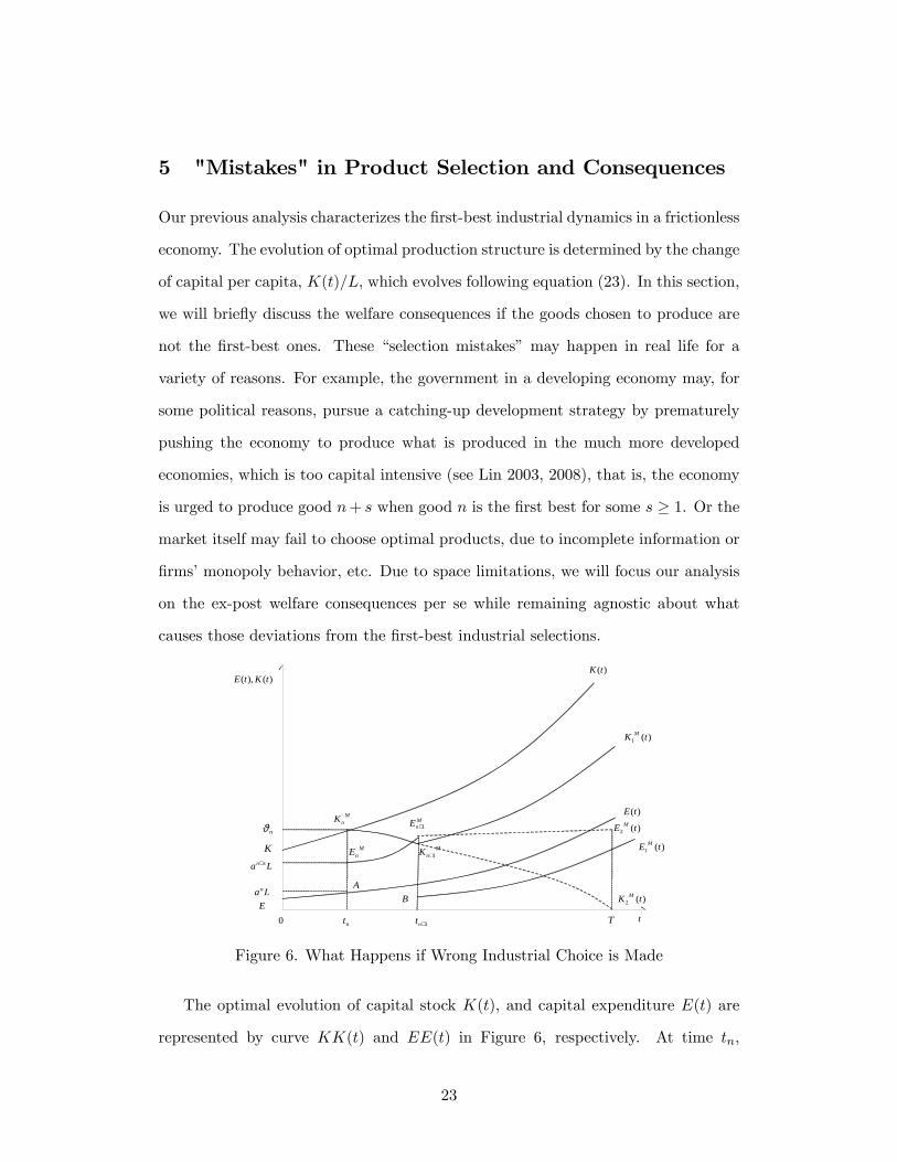
5 "Mistakes" in Product Selection and Consequences

Our previous analysis characterizes the �rst-best industrial dynamics in a frictionless

economy. The evolution of optimal production structure is determined by the change

of capital per capita, K(t)=L; which evolves following equation (23). In this section,

we will brie�y discuss the welfare consequences if the goods chosen to produce are

not the �rst-best ones. These �selection mistakes�may happen in real life for a

variety of reasons. For example, the government in a developing economy may, for

some political reasons, pursue a catching-up development strategy by prematurely

pushing the economy to produce what is produced in the much more developed

economies, which is too capital intensive (see Lin 2003, 2008), that is, the economy

is urged to produce good n+ s when good n is the �rst best for some s � 1. Or the

market itself may fail to choose optimal products, due to incomplete information or

�rms�monopoly behavior, etc. Due to space limitations, we will focus our analysis

on the ex-post welfare consequences per se while remaining agnostic about what

causes those deviations from the �rst-best industrial selections.

)(),( tKtE

tnt0

K

AB

1+nt T

)(tK

)(tE

E

MnK

)(1 tE M

)(2 tE M

)(1 tK M

MnK 1+

MnE

MnE 1+

Lan

La sn+

nϑ

)(2 tK M

Figure 6. What Happens if Wrong Industrial Choice is Made

The optimal evolution of capital stock K(t); and capital expenditure E(t) are

represented by curve KK(t) and EE(t) in Figure 6, respectively. At time tn;

23

K(tn) = #n and E(tn) = anL. It is optimal for the economy to start producing

good n+1 so that both good n and good n+1 should be produced at time interval

(tn; tn+1). Now suppose, for some unexpected and exogenous reasons, the economy

starts to produce goods n+s and n+s+1 during the period [tn; tn+1] for some s > 0:

s measures the magnitude of the industrial deviation. So at time tn; instead of using

E(tn) = anL; now suppose the economy chooses the expenditure E(tn) = an+sL and

maintains the same consumption growth rate ���� during this period. We use the

superscript �M�to denote all the variables after the economy is unexpectedly hit

by this �mistake.�What will the welfare consequence be?

Obviously at time tn, the aggregate consumption jumps from C(tn) to CM (tn).

Capital expenditure EM (t) now evolves as follows:

EM (t) =

�CM (tn)e

����(t�tn) � �

n+s(a� �)a� 1 L

�an+s+1 � an+s

�n+s+1 � �n+s

for any t 2 [tn; tn+1]. It is represented by curve EMn EMn+1 in Figure 6. Di¤erent

from equation (22), the transition equation of capital now becomes

�KM = �KM (t)�

�CM (tn)e

����(t�tn) � �

n+s(a� �)a� 1 L

�an+s+1 � an+s

�n+s+1 � �n+s, for any t 2 [tn; tn+1]:

(24)

If s is su¢ ciently large, the capital expenditure EM (t) exceeds �KM (t) and therefore

KM (t) declines in time period [tn; tn+1]: In that case, capital stock evolves along

the curve KMn K

Mn+1 which is not only below the �rst-best path KK(t) but also

decreasing. At time tn+1; KM (tn+1) < #n+1: Let us assume #h � KM (tn+1) � #h+1

for some 0 < h < n: Suppose at time t = tn+1 the government (or agents) in the

economy suddenly realizes that it made mistakes during the period [tn; tn+1]. What

should it do? There are two scenarios:

In Scenario 1, let us assume there is no adjustment cost to rectify the mistake.

The economy can freely re-optimize everything at t = tn+1 at given capital stock

24

K = KM (tn+1). Since #h � KM (tn+1) � #h+1, the economy will immediately

downgrade its production structure and start producing goods h and h + 1. The

corresponding capital expenditure EM (t+n+1) must be between ahL and ah+1L, and

the economy will then follow the optimal path as if it began with K = KM (tn+1):

The evolution paths for KM and EM are represented by KKMn K

Mn+1K

M1 (t) and

EAEMn EMn+1BE

M1 (t); respectively. Consumers enjoy the goods with qualities higher

than the optimal, n+ s and n+ s+ 1; in time period [tn; tn+1]; but have to adjust

the economy at a much lower level thereafter. The consumer�s life utility following

the mistaken path KKMn K

Mn+1K

M1 (t) certainly is lower than the optimum and can

be computed. Similarly, if the country saves more capital than the optimum, and

produces goods n � s and n � s + 1 in [tn; tn+1]; the country will re-optimize and

start to produce goods j and j+1 for some j � n+1 after t = tn+1; that also lowers

consumer�s lifetime total utility.

In Scenario 2, let us assume that the production structure can not be reversed

and maintain the full employment assumption. That is, when the economy starts

to produce good m; it can not produce any good with the quality lower than m

in the future. Full employment implies that the quantity of total consumption can

not decrease either. The industrial irreversibility may be due to the fact that the

physical capital used to produce high quality goods can not be reversed to produce

lower quality goods, or consumers who are used to consuming high-quality goods are

simply addicted to their consumer behavior, or political groups in current industries

may lobby against the structural adjustment. Under this assumption, the optimal

choice is to produce the lowest quality good constrained by the downward rigidity

constraint n � h + s + 1. Therefore, at each time point after t = tn+1 capital

expenditure E must always equal ah+s+1L. As too little capital is saved, KM (t)

continues to decline after tn+1 and will be exhausted at time T: The evolution

paths for KM and EM in Scenario 2 are represented by KKMn K

Mn+1K

M2 (t) and

EAEMn EMn+1E

M2 (t)T; respectively. Due to the adjustment rigidity, a short-term

25

mistake in production selection hurts the economy permanently by fully exhausting

all capital stock. The economy falls into a poverty trap without any growth and can

only a¤ord to produce good 0 forever after time T , if that is allowed after T .

Scenarios 1 and 2 provide two extreme cases for the e¤ect of mistakes in production

selection. Without adjustment cost, one period mistake to produce products above

the optimum lowers social welfare and postpones future product upgrading. When

the production structure is not reversible, however, one period over-expenditure in

capital may permanently degenerate the economy and destroy the hope for growth.

We can impose the same downward adjustment rigidity constraint on the economy

analyzed in the previous two sections, but nothing changes because this adjustment

constraint is simply not binding.

An intermediate adjustment cost function between Scenarios 1 and 2 may be

more realistic, but also more complicated to analyze. For example, we may assume

that right after time tn+1; capital stock K(t+n+1) = �([h � (n + 1)])K(tn+1) where

�(:) is the adjustment cost function. �(0) = 1, 0 � �(:) � 1, and �(:) becomes

larger if the absolute value of [h � (n + 1)] increases. If the economy maintains

its current production structures, there will be no adjustment cost. Otherwise, a

more radical adjustment incurs a higher adjustment cost. Scenario 1 represents

the case that �(:) � 1. For Scenario 2, it simply refers to the case that �(:) � 0 if

h�(n+1) < 0. When �(:) is intermediate, the economy may not immediately adjust

her production structures to the optimal products h and h+1. Instead, the country

may gradually downgrade its production structure to the optimal one determined

by its endowment structure. A thorough formal exploration is beyond the scope of

this paper, but studies of such optimal adjustment in production structures seem

very interesting, although quite limited in the literature.

In the real world, we observed successful examples of industrial upgrading in

Japan, South Korea, and Taiwan from the 1950s to the 1980s. That may be

partly attributed to the fact that the government in those economies pursued the

26

right industrial development policies that were consistent with their endowment

structures. However, there are many examples of less successful development with

�non-optimal�industrial dynamics in developing economies including China, India,

Russia, and many other Eastern European and Latin American countries during

various historical periods. These countries all erroneously pursued development

strategies that de�ed their comparative advantages by naively trying to quickly

mimic the production structure of the developed economies and, hence, prematurely

built too many heavy industries that were inconsistent with the economy�s endowment

structure. That ultimately resulted in serious economic stagnation and caused huge

welfare loss. Just as predicted by our above analysis, the welfare consequence is

even worse when the industrial adjustment is more costly. Indeed, we frequently

observe prolonged di¢ cult periods of adjustment in many economies undertaking

reforms. For instance, it has been more than 15 years since the regime switched

in Russia and the country�s endowment structure also dramatically deteriorated.

Nevertheless, military and some other heavy industries are still the main supporting

industries in that country (Lin 2003, 2009).

Serious welfare consequences may result from the government�s failure to recognize

that the optimal industries are actually endogenous to the development stage (capital

endowment). Such important policy implications, although indirectly derived from

this model, may not be obvious from the standard one-sector or multi-sector growth

models.

6 Conclusion

We have developed a tractable in�nite-horizon general-equilibrium model to analyze

the optimal industrial structure and its dynamics in a closed developing economy.

Explicit solutions are obtained to fully characterize the whole economic dynamics

(including the transitional dynamics), although the commodity space is in�nitely

27

dimensional. Our model generates an inverse-V-shaped dynamic pattern of industrial

change, which is widely observed in the real world but rarely, if ever, formalized in

growth models. The engine that drives this continuous structural change is the

increasing relative abundance of capital in the endowment structure. In a closed

economy, capital keeps accumulating because the capital goods are produced with

Arrow�s AK model technology, which can be interpreted as learning-by-doing in

the capital production. This endogenous technological change in the capital good

production gives us the sustained and constant economic growth in the aggregate

good consumption. However, since the industries are upgrading in a waxing-and-waning

fashion all the time, the growth rates of each individual industrial good are shown

to be changing along the process. We highlight the endogeneity of the industrial

structures and its dynamics: The optimal industrial choice and industrial dynamics

are dictated by the economy�s endowment structure and its change.

Economic growth and industrial upgrading are two crucial and integrated aspects

of sustained economic development. On the quantitative side, sustained economic

development requires the sustainable growth of per capita income; on the structural

side, sustainable economic development typically entails the continuous upgrading

and transformation of industries. Most existing growth models postulate the same

aggregate production function (with changing inputs and productivity) for all the

countries at di¤erent development stages, and, thus, naturally focus on the quantitative

side of economic aggregates, which have been guiding economists to conduct many

insightful policy studies such as how to boost human and physical capital accumulation

and how to enhance technological improvement, and so forth. However, the structural

side is largely ignored by these models. This perhaps accounts for the more

serious shortage of academic and policy research related to structural changes in

development: How to help the economy identify the optimal products and industries

to develop at each di¤erent development stage, which kind of �nancial institutions

can best serve the corresponding industrial structures at di¤erent stages, how to

28

facilitate the structural transformation in the process of labor and capital reallocation

across industries, how openness may a¤ect a country�s industry upgrading, and,

consequently, what the optimal industrial, �nancial, trade, and many other macroeconomic

policies should be at di¤erent development stages, so on and so forth. We hope the

model developed in this paper may serve as a useful starting point to address all

these fundamental issues.

References

[1] Acemoglu, Daron, and Veronica Guerrieri. 2008. "Capital Deepening andNonbalanced Economic Growth." Journal of Political Economy 116 (June):467-498.

[2] Aghion, Philippe and Peter Howitt. 1992. "A Model of Growth ThroughCreative Destruction." Econometrica, 60(2): 323-351.

[3] Akamatsu, Kaname. 1962. "A Historical Pattern of Economic Growth inDeveloping Countries. In: The Development Economies, Tokyo, PreliminaryIssue No. 1, pp.3-25.

[4] Barro, Robert J. and Sala-i-Martin, Xavier. 2004. Economic Growth. SecondEdition. Cambridge: The MIT Press.

[5] Buera, Francisco J. Buera and Joseph P. Kaboski. 2009. "The Rise of the ServiceEconomy," NBER working paper #14822.

[6] Caselli, Francesco, and John Coleman. 2001. "The U.S. StructuralTransformation and Regional Convergence: A Reinterpretation." Journalof Political Economy 109 (June): 584-617.

[7] Chenery, Hollis B. 1960. "Patterns of Industrial Growth," American EconomicReview 50 (September): 624-654.

[8] � � �. 1961. "Comparative Advantage and Development Policy." AmericanEconomic Review 51 (March): 18-51

[9] � � , Robinson Sherman, and Syrquin Moshe. 1986. Industrialization andGrowth: A Comparative Study. New York: Oxford University Press (forWorld Bank)

[10] Gollin, Douglas, Stephen Parente, and Richard Rogerson. 2002. "The Roleof Agriculture in Development." American Economic Review, Papers andProceedings 92(May):160-164

[11] Grossman, Gene, and Elhanan Helpman. 1991a. "Quality Ladders in the Theoryof Growth." Review of Economic Studies 58 (January): 43-61

[12] � � . 1991b. "Quality Ladders and Product Cycles." Quarterly Journal ofEconomics 106(May): 557-586

29

[13] Hansen, Gary and Edward Prescott. 2002. "Malthus To Solow." AmericanEconomic Review 92 (September): 1205-1217

[14] Hayami, Yujiro, and Yoshihisa Godo. 2005. Development Economics: From thePoverty to the Wealth of Nations. Oxford University Press

[15] Houthakker, H. S. 1956. "The Pareto Distribution and Cobb-GouglassProduction Faction in Activity Analysis," Review of Economic Studies23(1): 27-31

[16] Kamien, Morton I. and Nancy L. Schwartz. 1991. Dynamic Optimization: TheCalculus of Variations and Optimal Control in Economics and Management.New York: Elsevier Science Publishing Co. Inc.

[17] Kojima, Kiyoshi. 2000. "The Flying Geese Model of Asian EconomicDevelopment: Origin, Theoretical Extensions, and Regional PolicyImplications." Journal of Asian Economics 11: 375-401

[18] Kongsamut, Piyabha, Rebelo, Sergio and Danyang Xie. 2001. "BeyondBalanced Growth." Review of Economic Studies 68: 869-882

[19] Krugman, Paul. 1979."A Model of Innovation, Technology Transfer, and theWorld Distribution of Income." Journal of Political Economy 87(April):253-266

[20] Kuznets, Simon. 1966. Moder Economic Growth: Rate, Structure, and Spread.New Heaven: Yale University Press

[21] Lagos, Ricardo. 2006. "A Theory of TFP." Review of Economic Studies,73(October): 983-1007

[22] Laitner, John. 2000. "Structural Change and Economic Growth." Review ofEconomic Studies 67(July): 545-561

[23] Leamer, Edward. 1987. "Path of Development in Three-Factor n-Good GeneralEquilibrium Model." Journal of Political Economy 95 (October): 961-999

[24] Lin, Justin Yifu. 2003. "Development Strategy, Viability, and EconomicConvergence." Economic Development and Cultural Change 51(January):277-308

[25] � � �. 2009. Marshall Lectures: Economic Development and Transition:Thought, Strategy, and Viability. London: Cambridge University Press

[26] Lucas, Robert. 2004. "Life Earnings and Rural-Urban Migrations." Journal ofPolitical Economy 112: S29�S58

[27] � �.2009. "Trade and the Di¤usion of the Industrial Revolution," AmericanEconomic Journal: Macroeconomics 1(1): 1-25

[28] Maddison, Angust. 1980. "Economic Growth and Structural Change inAdvanced Countries," in Irving Leveson and Jimmy W. Wheler, eds.,Western Economies in Transition: Structural Change and AdjustmentPolicies in Industrial Countries. London: Croom Helm

30

[29] Mastuyama, Kiminori. 1992. "Agricultural Productivity, ComparativeAdvantage and Economic Growth." Journal of Economic Theory58(December): 317-334

[30] � � �. 2002. "Structural Change", Prepared for New Palgrave Dictionary

[31] Murphy, Kevin, Andrei Shleifer, and Robert Vishny. 1989. "Industrializationand Big Push," Journal of Political Economy 97(October): 1003-1026

[32] Ngai, L. Rachel, and Christopher A. Passarides. 2007. "Structural Change in aMulti-Sector Model of Growth." American Economic Review 97 (January):429-443

[33] Solow, Robert. 1956. "A Contribution to the Theory of Economic Growth,"Quarterly Journal of Economics 70 (February): 65-94

[34] Schotter, Peter. 2003. "One Size Fits All? Heckscher-Ohlin Specialization inGlobal Production," American Economic Review 93(June): 686-708

[35] Schumpeter, Joseph. 1942. Capitalism, Socialism and Democracy. New York:Harper and Brothers

[36] Stokey, Nancy. 1988. "Learning by Doing and the Introduction of New Goods."Journal of Political Economy 96 (August): 701-717

[37] Ventura, Jaume. 1997. "Growth and Interdependence." Quarterly Journal ofEconomics, February: 57-84

[38] Vernon, Raymond. 1966. "International Investment and International Trade inProduct Cycle." Quarterly Journal of Economics: 190-207

[39] World Bank Commission on Growth and Development. 2008. The GrowthReport: Strategies for Sustained Growth and Inclusive Development.Washington, DC: World Bank Publications

31

7 Appendix

7.1 Appendix 1

In Appendix 1, we show that in the competitive equilibrium, if two di¤erent industrialgoods are produced simultaneously, these two goods have to be adjacent in quality.

Proof: By contradiction. Suppose the above statement is not true, then therecan exist some good j and good m such that 1 � j � m � 2 , and cj and cm areboth strictly positive in the equilibrium. Then

MRSm;j = �m�j =

amr + w

ajr + w;

which meansr

w=

�m�j � 1aj(am�j � �m�j)

:

Now we show that at this relative price, good j + 1 strictly dominates good j, thatis

MRSj+1;j �aj+1r + w

ajr + w= ��

aj+1 �m�j�1aj(am�j��m�j) + 1

aj �m�j�1aj(am�j��m�j) + 1

> 0;

which is equivalent to

�n � 1an � �n <

1� ��� a , for some integer n � m� j � 2: (25)

This is true because

�n � 1an � �n =

(�� 1)Pn�1i=0 �

i

�n��a�

�n � 1� =(�� 1)

Pn�1i=0 �

i

�n��a�

�� 1�Pn�1

i=0

�a�

�i=

(�� 1)Pn�1i=0 �

i

�n�1 (a� �)Pn�1i=0

�a�

�i = (�� 1)Pn�1i=0 �

i

(a� �)Pn�1i=0 �

ian�1�i<�� 1a� � for any n � 2:

Therefore, it contradicts that good j is produced and consumed.It�s straightforward to show that it is possible to have both good 0 and good 1

under some conditions.Now we need to show that if some good n � 2 is the only industrial good that�s

produced, then good 0 can not be produced. From (6), we know that the householdwould strictly prefer good n to good n+ 1 if

�n+1�n

<pn+1pn

=w + an+1r

w + anr; for n = 1; ::

or equivalently,r

w>

�� 1an+1 � �an ; (26)

32

and good n is strictly preferred to good n� 1 if and only if

r

w<

�� 1an � �an�1 : (27)

This means�� 1

an+1 � �an <r

w<

�� 1an � �an�1 : (28)

If c0 > 0, then �n = w+anrw because of (6), that is

�n � 1an

=r

w:

So we must have�� 1

an+1 � �an <�n � 1an

<�� 1

an � �an�1 ;

where the second inequality is equivalent to

�n � 1�� 1 <

a

a� �:

However, since a�1 > �, there will exist no integer n � 2 that can satisfy the aboveinequality because the left hand side is no smaller than � + 1. This implies thatc0 = 0.

7.2 Appendix 2

In Appendix 2, we solve for the initial value of total consumption C(0) when #0 <K(0) � #1, and also show how to derive the threshold values for #i; i = 0; 1; 2; :::.The transversality condition is derived from

limt!1

H(t) = 0;

so

limt!1

�C(t)1�� � 11� � e��t + �n(t);n(t)+1

��K(t)� En(t);n(t)+1(C(t))

��= 0:

33

Note that

limt!1

�C(t)1�� � 11� � e��t + �n(t);n(t)+1

��K(t)� En(t);n(t)+1(C(t))

��= limt!1

"C(0)1��e

����(1��)t

1� � e��t + �n(t);n(t)+1��K(t)� En(t);n(t)+1(C(t))

�#= limt!1

h�n(t);n(t)+1

��K(t)� En(t);n(t)+1(C(t))

�i= limt!1

(�(0)e

��t

"�K(t)�

"C(0)e

����t � �

n(t)(a� �)a� 1 L

#an(t)+1 � an(t)

�n(t)+1 � �n(t)

#)

= limt!1

(�(0)

"�K(t)e��t �

��e

��t(a� �)a� 1 L

�an(t)+1 � an(t)

�� 1

#)= limt!1

K(t)e��t;

thus we must have limt!1

K(t)e��t = 0. When t 2 [t0 = 0; t1],

E(t) =a

�� 1(C(t)� L) =a

�� 1(C(0)e����t � L);

Correspondingly,

�K = �K(t)� E(C(t)) = �K(t)� a

�� 1(C(0)e����t � L)

Solving this �rst-order di¤erential equation with the conditionK(0) = K0, we obtain

K(t) =�aC(0)

��1���� � �

e����t +

�aL� (�� 1) +

"K0 +

aC(0)��1

���� � �

+aL

� (�� 1)

#e�t; (29)

from which we obtain

K(t1) =� a�L��1

���� � �

+�aL

� (�� 1) +"K0 +

aC(0)��1

���� � �

+aL

� (�� 1)

#��L

C(0)

� �����

: (30)

When t 2 [tn; tn+1] for 8n � 1, we have

K(t) = � an+1 � an

�n+1 � �n

24C(0)e ���� t����� � �

� + �n(a� �)L� (a� 1)

35+ �n:n+1e�t: (31)

which gives

�n:n+1 =

��nL

C(0)

�������

8<:K(tn) + an+1 � an�� 1 L

24 1����� � �

� + (a� �)� (a� 1)

359=; (32)

34

Therefore, we obtain equation (23). Substituting t = tn+1 =log �

n+1LC(0)

����

into (23), we

obtain

K(tn+1) = ������K(tn) +

an+1 � an�� 1 L

24 � ����� � ������ � �

� + (a� �)(� ����� � 1)

� (a� 1)

35Using the recursive induction, we get

K(tn) = �(n�1)����� K(t1)+(a�1)B�

(n�2)�����

a

�1�

�a�

�������n�1�

1� a�������

; for any n � 2 (33)

where B is a parameter de�ned as

B � L

�� 1

264� ����� � ����� � �

+(a� �)

��

����� � 1

��(a� 1)

375 :The transversality condition lim

t!1K(t)e��t = 0 implies that

�������K(t1) + (a� 1)B�

�2�����

a

1� a�������

= 0;

so

K(t1) = �(a� 1)B�

������ a

1� a�������

: (34)

To make the analysis rigorous and relevant, we will have impose two additionalassumptions.

a < ������ ; (35)

and

� >�(a� �)

��

����� � 1

���a� �

������(1� �) + (a� �)

��

����� � 1

� : (36)

(35) is needed to ensure #0 > 0. It says that capital accumulation speed � has tobe su¢ ciently large relative to the capital intensity parameter a so that industrialupgrading is indeed happening. (36) ensures #1 � K(t1) > 0 and B < 0. Note that(36) guarantees that � > �:

35

According to (30), we have24K0 + aC(0)

(�� 1)����� � �

� + aL

� (�� 1)

35� �L

C(0)

� �����

=a�L

(�� 1)����� � �

� + aL

� (�� 1) �(a� 1)B�

������ a

1� a�������

. (37)

We can verify that the right hand side is strictly positive. Observe that the lefthand side is a strictly decreasing function of C(0), therefore we can uniquely pindown the optimal C�(0). (37) immediately implies @C

�(0)@K0

> 0 and @C�(0)@L > 0.

Note that (34) implies that K(t1) does not depend on K(0), therefore (33) tellsthat K(tn) for all n � 1 are independent from K(0):

To ensure C�(0) � �L, we need K0 � � (a�1)B������� a

1�a�������

, which requires

K0 � #1 � �������� a

1� a�������

1

�� 1

264��a� �

������(1� �) + ���

� (a� �)��

����� � 1

������ � �

��

375L:We also need to ensure C�(0) > L, which requires24K0 + aL

(�� 1)����� � �

� + aL

� (�� 1)

35� ����� >

a�L

(�� 1)����� � �

�+ aL

� (�� 1)�(a� 1)B�

������ a

1� a�������

;

that is

K0 > #0 �a

(�� 1)

�����

���� � �

��

264�1� �1�

������(1� �

����� )

�������1� a�

�������

375L:7.3 Appendix 3

In Appendix 3, we prove that there exists a series of constant numbers, #0; #1; � � � ; #n; #n+1; � � � ;if 0 < K(0) � #0; the economy will start from producing good 0 only until the capitalstock reaches #0; if #0 < K(0) � #1; the economy will start from producing goods0 and 1; if #n < K(0) � #n+1; the economy will start from producing goods n andn+ 1: Furthermore, K(tn) = #n for any value of K(0) < #n:

Now let us characterize the solution to the above dynamic problem when K0 2(0; #0] while keeping all the other assumptions unchanged. The economy must startby producing good 0 only. The discounted-value Hamiltonian with the Lagrangian

36

multipliers is the following

H0 =C(t)1�� � 11� � e��t + �0�K(t) + �

00(L� C(t)):

First order condition and K-T condition are

C(t)��e��t = �00;

�00(L� C(t)) = 0;L� C(t) = 0 when �00 > 0:

and

�0 = �@H0@K

= ��0�:

They immediately imply that C�(t) = L: This is because labor entails no utility costfor the household therefore C(t) must be equal to L when only good 0 is produced.No capital is used for production and therefore

�K(t) = �K(t):

When capital stockK exceeds #0 by an in�nitessimal amount, the economy producesboth good 0 and good 1. From that point on, the problem is exactly the same asthe one we have just solved in the main text. Let t0 denote the time point when Kequals #0. Then

K0e�t0 = #0,

so t0 =log

#0K0� . Therefore

C�(t) =

(L; when t � t0

Le����(t�t0); when t > t0

:

Let tj denote the time point when only good j is produced, for any j � 1. Observethat Le

����(tj�t0) = C(tj) = �

jL, so tj = t0 +�� log ����

�j.

Correspondingly, the capital stock on the equilibrium path is given by

K(t) =

8>><>>:K0e

�t; for t 2 [0; t0]� aL��1

������e����(t�t0) + �aL

�(��1) +

�#0 +

aL��1

������+ aL

�(��1)

�e�(t�t0); for t 2 [t0; t1]

F (t); for t 2 [tn; tn+1]; any n � 1

;

37

where

F (t) � � an+1 � an

�n+1 � �n

24 Le����t�

���� � �

� + �n(a� �)L� (a� 1)

35+ [�n]

������

8<:K(tn) + an+1 � an�� 1 L

24 1����� � �

� + (a� �)� (a� 1)

359=; e�(t�t0);t0 =

log#0K0� , tj = t0 +

�� log ����

�j for any j � 1, K(t0) = #0; and K(tn) is exactly the

same as before for any n � 1.Using the similar algorithm, we can fully specify the transitional dynamics when

K0 > #1. We have already provided an algorithm to compute #i for i � 2 in themain text by using (33). An alternative way is to back out the threshold value #ifrom the corresponding transversality conditions for any i � 2. It can be veri�edthat all these values are the same for both algorithms, and that all these thresholdvalues are independent of K0. In other words, K0 only has level e¤ect (i.e. it onlya¤ects C(0)) but no speed e¤ect on industrial upgrading. The main reason is thatthis economy is perfectly stationary, thus di¤erent initial capital levels only translateinto di¤erent initial aggregate consumption and initial industrial structures.

7.4 Appendix 4

This appendix is to illustrate that the assumption of Leontief production functionis not crucial for the main qualitative results. Suppose the production function isCobb-Douglass for any industry level i = 1; 2; ::. That is,

Yi = AiK�ii L

1��ii ;

where capital share �i strictly increases with i but always belongs to interval [0; 1] .The total output is

Pi Yi. Consider the simplest static case in which there are only

two industries: i = 1 and 2. The total labor and capital endowment are L and E.We can easily prove the following proposition:

De�ne

k�1 �"��1�2

��2 �1� �11� �2

�1��2 �A1A2

�# 1�2��1

;

k�2 �"��1�2

��1 �1� �11� �2

�1��1 �A1A2

�# 1�2��1

:

(a) If EL � k�1, the economy only produces good 1 with the total output F (E;L) =

A1E�1L1��1 .

38

(b) If k�1 <EL < k

�2; then both goods will be produced with

L�1 =

1�

EL � k

�1

k�2 � k�1

!L; L�2 =

EL � k

�1

k�2 � k�1L;

K�1 = k�1L

�1; K

�2 = k

�2L

�2:

The implied aggregate production function is

F (E;L) =

264�A1 (k

�1)�1 � A2(k�2)

�2�A1(k�1)�1

k�2�k�1k�1

�L

+A2(k�2)

�2�A1(k�1)�1

k�2�k�1E

375 :(c) If KL � k�2, the economy only produces good 2 with total output F (E;L) =A2E

�2L1��2 .In addition, the aggregate production function F (E;L) is constant return to

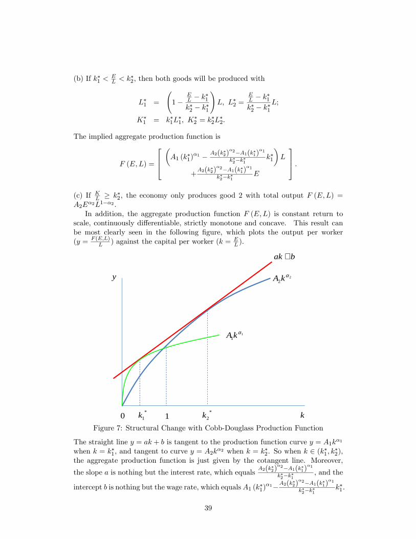
scale, continuously di¤erentiable, strictly monotone and concave. This result canbe most clearly seen in the following �gure, which plots the output per worker(y = F (E;L)

L ) against the capital per worker (k = EL ).

11

αkA

22

αkA

bak +

y

0 1 *2k*

1k kFigure 7: Structural Change with Cobb-Douglass Production Function

The straight line y = ak + b is tangent to the production function curve y = A1k�1

when k = k�1, and tangent to curve y = A2k�2 when k = k�2. So when k 2 (k�1; k�2),

the aggregate production function is just given by the cotangent line. Moreover,

the slope a is nothing but the interest rate, which equalsA2(k�2)

�2�A1(k�1)�1

k�2�k�1, and the

intercept b is nothing but the wage rate, which equalsA1 (k�1)�1�A2(k�2)

�2�A1(k�1)�1

k�2�k�1k�1.

39

So the interest rate and wage rate both keep constant when both good 1 and good 2are produced. The same logic can be extended to the case with an in�nite-dimensionalcommodity space, in which case the aggregate production function is simply theconvex envelope of all the individual industry production functions although thosein�nitely many tangent points seem harder to analytically characterize in a generaland very neat way as in the Leonteif production function case. This problem is alsocarried into the dynamic analysis, but it should be clear that the main qualitativeresults would still remain valid.

40