Endogenous transportation technology in a Cournot

differential game with intraindustry trade

Luca Colombo, Luca Lambertini *, Andrea Mantovani

Department of Economics, University of Bologna, Strada Maggiore 45, 40125 Bologna, Italy

Received 12 February 2007; received in revised form 9 August 2007; accepted 7 April 2008

Abstract

We investigate a dynamic Cournot duopoly with intraindustry trade, where firms invest in R&D to reduce the level of iceberg transportation

costs. We adopt both open-loop and closed-loop equilibrium concepts, showing that a unique (saddle point) steady state exists in both cases. In the

open-loop model, optimal investments and the resulting efficiency of transportation technology are independent of the relative size of the two

countries. On the contrary, in the closed-loop case firms’ R&D incentives are driven by the relative size of the two countries. Policy implications are

also evaluated.

# 2008 Elsevier B.V. All rights reserved.

JEL classification: D43; F12; F13; L13; O31

Keywords: R&D; Differential games; Transport and communication costs; Intraindustry trade

www.elsevier.com/locate/jwe

Available online at www.sciencedirect.com

Japan and the World Economy 21 (2009) 133–139

1. Introduction

Transport and communication costs are at the heart of

many international trade issues because they put a wedge on

transactions across borders. While the traditional view

considered national borders affecting trade because their

existence was associated with discriminatory policies and

mere physical distance, more recent interpretations include a

broad category of features such as language, different legal

systems across borders, local consumer tastes, i.e., everything

that may constitute an economic and social impediment for

the exporting firm. Empirical research on trade carried out by

McCallum (1996) revealed a surprisingly high degree of

market fragmentation that gives rise to border effects and to

the so-called ‘‘home bias’’ effect. Obstfeld and Rogoff (2000)

referred to the home bias as one of the ‘‘six major puzzles in

international macroeconomics’’. In their view, the interaction

between iceberg transport costs and the elasticity of

* Corresponding author at: ENCORE, Faculty of Economics & Econometrics,

University of Amsterdam, Roetersstraat 11, 1018 WB Amsterdam, The Nether-

lands.

E-mail addresses: colombo@spbo.unibo.it (L. Colombo),

luca.lambertini@unibo.it (L. Lambertini), a.mantovani@unibo.it

(A. Mantovani).

0922-1425/$ – see front matter # 2008 Elsevier B.V. All rights reserved.

doi:10.1016/j.japwor.2008.04.001

substitution between domestic and foreign goods accounts

for much of the observed home bias. Anderson and

Marcouiller (1999) proposed a different explanation for the

home bias, relying on the consideration that the rule of law is

much weaker when trade is international. Along the same

line, Turrini and van Ypersele (2002) pointed out that the

home bias can be explained by differences in legal systems, so

that legal costs are higher when business is done abroad rather

than at home.

Nonetheless, the issue of transport costs has not received

sufficient attention in the literature, perhaps because of steadily

declining communication and shipment costs.1 However, the

persistence of many home biases confirms that the question of

transport costs is not a secondary one and needs further and

deeper investigations.

In this paper, we consider a duopoly Cournot game with two

firms located in different countries that open up to trade but face

1 Harley (1980) and O’Rourke and Williamson (1999) document the sharp

decline in both ocean and overland transportation costs. Another example is the

widespread use of Internet to facilitate sales and ultimately reduce the distance

between firms and consumers. The possibility of placing on-line orders on the

web sites of Amazon or Blackwell as well as buying train or flight tickets on the

web sites of railways and airlines all over the world has brought about a

significant reduction in global trade costs.

L. Colombo et al. / Japan and the World Economy 21 (2009) 133–139134

an additional cost when delivering abroad. According to the

previous discussion, these costs are not only due to physical

distance, but also to the access to a foreign network of

communication and distribution. We allow firms to invest in

Transport and Communication R&D (TCRD) to improve the

penetration into foreign markets, thus increasing their market

share.

Both the open-loop and the closed-loop equilibria are

investigated.2 In the former, the resulting steady state

investment efforts and the efficiency levels of transportation

technologies depend only upon time discounting, deprecia-

tion and the efficiency of TCRD. This is due to the fact that, in

the open-loop setting, firms design an investment plan at the

outset and stick to it until they reach the steady state,

regardless of the strategic interaction taking place in between.

Accordingly, the relative size of the two countries does not

influence the investment behaviour and the resulting

performance of firms’ transportation technologies at equili-

brium. On the contrary, in the closed-loop equilibrium firms

explicitly account for strategic interaction through reciprocal

feedback effects at any point in time. This yields optimal

investment efforts and equilibrium technologies that do

depend upon the relative size of the two markets. In particular,

each firm’s optimal investment is positively affected by the

size of the foreign country, all else equal. This can be labelled

as a ‘foreign market effect’, for the sake of contrasting this

finding with the well known ‘home market effect’ whereby a

firm located in the larger market sells more than the firm

located in the smaller market (see Krugman, 1990, inter alia).

When firms only control sales in order to maximise profits,

then, intuitively, market shares on the international market

place go along with the relative size of countries. However, if

firms are required or allowed to endogenously determine their

respective ability to reach the foreign market, then the size of

the latter may matter more than the size of the home market.

All this applies for a given efficiency level of transportation

technologies, which, however, is endogenously determined by

R&D efforts.

Once we take this into account and fully characterise the

steady state equilibrium, we find that the larger is the home

market, the lower will be the efficiency of the transportation

technology employed by a firm in the closed-loop steady state

equilibrium. This is the outcome of the foreign market effect

operating throughout the game, before firms indeed reach the

steady state. The stationarity requirement entails that in the

long run equilibrium only, the firm located in the larger

country invests more than the rival in the smaller country. This

reveals the presence of a ‘home market effect’ operating

exclusively at equilibrium. This result is in sharp contrast with

the conclusion obtaining from the static game (Lambertini

and Rossini, 2006), where the firm based in the larger country

has a lower incentive to invest in order to improve its

2 For an introduction to differential oligopoly games, see Cellini and Lam-

bertini (2003). For a more detailed treatment of differential game theory, see

Dockner et al. (2000).

transportation technology, as compared to the rival located in

the smaller country.

A domestic policy maker aiming at improving his country’s

social welfare may adopt two alternative measures (or a

combination of both). He may modify either the instantaneous

cost of investment, or the efficiency of the R&D technology,

through subsidies or taxation. In both cases, a taxation policy

should be adopted so as to reduce excess investment

characterising the closed-loop equilibrium.3

The remainder of the paper is organized as follows. The

setup is laid out in Section 2. Open-loop and closed-loop

equilibria are investigated in Section 3. Section 4 analyses

policy implications. Concluding remarks are given in Section 5.

2. The model

We consider a model of bilateral trade between two firms

selling a homogeneous good. We assume that firm i is located in

country A while firm j is located in country B. Market

competition takes place as a Cournot game where each firm

chooses the profit maximizing quantity for each country

separately (Brander, 1981). Time is continuous and denoted by

t, with t2 ð0;1Þ.Firms face an additional transport cost only when

shipping the final good abroad. This amounts to saying that

transport costs only affect international trade. We model

transportation costs as in Samuelson (1954), i.e. using the

iceberg metaphor.

Consider the following indirect demand system:

pAðtÞ ¼ aA � qiAðtÞ �q jAðtÞs jðtÞ

(1)

pBðtÞ ¼ aB � q jBðtÞ �qiBðtÞsiðtÞ

(2)

where aA and aB stand for market-sizes, both supposed to be

constant over time; qiAðtÞ (q jBðtÞ) denotes the quantity pro-

duced by firm i ( j) for domestic consumption and q jAðtÞ (qiBðtÞ)represents the quantity produced by firm j (i) for foreign

consumption; q jAðtÞ=s jðtÞ, with s jðtÞ> 1 8 t2 ½0;1Þ, repre-

sents the proportion of firm j’s exported good that arrives in

country A at time t, and similarly for qiBðtÞ=siðtÞ. Firms face the

possibility of investing in TCRD to increase such proportion; in

particular, TCRD carried out by firm i (j) acts by reducing the

iceberg cost siðtÞ (s jðtÞ).Before proceeding, notice that in the demand system (1) and

(2) trade costs recall product differentiation (Singh and Vives,

1984), where the demand function of good i would write pi ¼a� qi � gq j; with g 2 0; 1½ �measuring product substitutability.

The analogy between parameter g in Singh and Vives (1984)

3 This phenomenon is widely accounted for in the literature since Brander

and Spencer (1983). We do not dwell upon the possibility for a policy maker to

adopt tariffs or quotas, in view of the recent guidelines of GATT and WTO.

However, for a dynamic approach to such trade policy measures, see Calzolari

and Lambertini (2006, 2007).

L. Colombo et al. / Japan and the World Economy 21 (2009) 133–139 135

and the reciprocal of the state variable siðtÞ in the present model

is clear. However, while there firms profit from any increase in

product differentiation, here they aim at reducing trade costs as

much as possible. Given the analogy between g and 1=siðtÞ; in

the present model firms behave as if they were aiming at

homogenising consumer tastes across borders. This may be a

sound interpretation of those real-world cases where consumers

hesitate in front of newly imported products, and the iceberg

cost summarises not only trade costs but also those costs

associated with advertising campaigns.

On the supply side, production exhibits constant return to

scale. For the sake of simplicity, we normalize unit costs to

zero. Instantaneous profits are then given by:

piðtÞ ¼ pAðtÞqiAðtÞ þ pBðtÞqiBðtÞsi tð Þ � b kiðtÞ½ �2 (3)

p jðtÞ ¼ pBðtÞq jBðtÞ þ pAðtÞq jAðtÞs j tð Þ � b k jðtÞ

� �2(4)

where kiðtÞ and k jðtÞ, respectively, represent the amount of

effort made by firm i and firm j at time t in order to reduce the

percentage of quantity lost on the way. Parameter b> 0 is an

inverse measure of TCRD productivity.

As a result of such activities, each firm increases the fraction

of good that reaches foreign market. We assume that siðtÞ and

s jðtÞ evolve (in particular, always decrease) over time

according to the following kinematic equations:

siðtÞ ¼@siðtÞ

@t¼ ½akiðtÞ � dsiðtÞ�½1� siðtÞ� (5)

s jðtÞ ¼@s jðtÞ

@t¼ ½ak jðtÞ � ds jðtÞ�½1� s jðtÞ� (6)

where d2 ½0; 1� denotes the depreciation rate, which is common

to both firms and constant over time; a> 0 is a constant

parameter positively affecting the accumulation process.4

We assume that firm i aims at maximizing the discounted

profit flow:

PiðtÞ ¼Z 1

0

piðtÞ e�rtdt (7)

w.r.t. controls kiðtÞ and the market variables qiAðtÞ and qiBðtÞ,under the constraint given by the state dynamics (5). Firm j

follows an analogous dynamic optimization program. The

discount rate r> 0 is assumed to be constant and common

to both firms.

3. Solution of the game

The current value Hamiltonian function for firm i writes:

Hi ¼ e�rt piðtÞ þ liiðtÞsiðtÞ þ li jðtÞs jðtÞ� �

dt (8)

4 The functional form adopted for the state Eqs. (5) and (6) ensures the

concavity of the profit-maximisation problem. Moreover, the term ½1� siðtÞ�implies that siðtÞ ¼ 0 when si ¼ 1.

where liiðtÞ ¼ miiðtÞert and li jðtÞ ¼ mi jðtÞert;miiðtÞ being the

co-state variable associated with siðtÞ. Firms play simulta-

neously. Firm i’s first-order conditions (FOCs) on controls

are5:

@Hi

@qiI

¼ 0) qiI ¼1

2aI �

q jI

s j

� �; I ¼ A;B (9)

@Hi

@qiJ

¼ 0) qiJ ¼si

2aJ � q jJ

� ; J ¼ A;B (10)

@Hi

@ki¼ 0) lii ¼

2bki

a 1� sið Þ (11)

along with the transversality and initial conditions:

limt!1

miisi ¼ 0; sið0Þ> 1: (12)

Note that the above FOCs do not contain li j, therefore we set

li j ¼ 0 for all t2 0;1½ Þ. Moreover, (9) contains s j, i.e., the

state variable of the rival, meaning that the open-loop solution

and the closed-loop memoryless solution do not coincide.

Consequently, we deal with the two solution concepts.

3.1. Open-loop Nash equilibrium

The outcome of the open-loop game is summarised by the

following:

Proposition 1. The open-loop game reaches a unique steady

state at:

kOLi ¼

rþ d

a; sOL

i ¼rþ d

d:

The equilibrium kOLi ; sOL

i

� �is a saddle point.

Proof. Under the open-loop solution concept, we can specify

the firm i’s co-state equation as follows:

� @Hi

@si¼ lii � rlii, (13)

lii ¼qiJ si aJ � q jJ

� � 2qiJ

� �þ lii rþ aki � d 2si � 1ð Þ½ �s3

i

s3i

:

Now, by using (11), one obtains the dynamics of investment:

ki ¼a

2blii 1� sið Þ � liisi½ � (14)

which can be simplified by using the co-state Eq. (13) and the

system (9) and (10):

ki ¼ ki rþ d� dsið Þ (15)

5 For the sake of brevity, in the remainder we omit the indication of time as

well as exponential discounting.

L. Colombo et al. / Japan and the World Economy 21 (2009) 133–139136

The steady state equilibrium requires fki ¼ 0; si ¼ 0g,yielding:

kOLi ¼

rþ d

a; sOL

i ¼rþ d

d(16)

Since under open-loop solution concept, by definition,

feedback effects are not accounted for, the equilibria we find are

such that the size of the country does not play any role. Indeed,

kOLi and sOL

i depend only upon intertemporal parameters.6

As to the issue of stability, on the basis of symmetry, we can

look at a single firm in isolation. Using the two differential

Eqs. (5) and (15), we can write the Jacobian matrix of firm i:

JOL ¼

@si

@si

@si

@ki

@ki

@si

@ki

@ki

2664

3775 ¼ �dþ 2dsi � aki a 1� sið Þ

�dki rþ d� dsi

�

The trace and determinants of JOLare:

Tr JOL�

¼ rþ 1� d> 0

D JOL�

¼ rd 2si � 1ð Þ � arki þ d2 si 3� 2sið Þ � 1½ �

which, evaluated at kOLi ; sOL

i

� �; simplifies as follows:

D JOL�

¼ �r rþ dð Þ< 0:

This concludes the proof. &

Equilibrium outputs are:

qOLiA ¼

aA

3; qOL

iB ¼aBsOL

i

3¼ aB rþ dð Þ

3d

qOLjA ¼

aAsOLj

3¼ aA rþ dð Þ

3d; qOL

jB ¼aB

3

(17)

while profits are:

pOLi ¼

a2A þ a2

B

9� b rþ dð Þ2

a2> 0 iff

a2A þ a2

B

9>

b rþ dð Þ2

a2:

(18)

3.2. Closed-loop Nash equilibrium

Here, we take into account the feedback between player i’s

strategy and player j’s state variable. This will lead to an

equilibrium characterized by subgame perfection. The first-

order conditions on controls are (9)–(11).

We specify firm i’s co-state equation containing the

feedback effects:

� @Hi

@si� @Hi

@q jJ

@q�jJ@si¼ lii � rlii (19)

along with the transversality and initial conditions:

limt!1

miisi ¼ 0; sið0Þ> 1: (20)

6 This can be shown to hold as well in a similar setup without trade (see

Colombo et al., 2004).

The partial derivatives appearing in (19) are:

@Hi

@si¼

2q2iJ � qiJ aJ � q jJ

� si þ lii 2si � 1ð Þd� aki½ �s3

i

s3i

(21)

@Hi

@q jJ

¼ � qiJ

si;@q�jJ@si¼ qiJ

2s2i

(22)

Optimal output levels are as in (17), i.e., qCLiI ¼ aI=3 and

qCLiJ ¼ aJsCL

i =3. Now, by using (14), (17) and the co-state

Eq. (19), we can write:

ki ¼36bkisi r� dsi þ dð Þ � a2

J si � 1ð Þa36bsi

(23)

However, steady state solutions are cumbersome, therefore

they cannot be intuitively interpreted. Hence, we proceed as

follows. We impose ki ¼ 0 to determine an equilibrium relation

between ki and si:

kCLi sið Þ ¼

a2J si � 1ð Þa

36bsi r� d si � 1ð Þ½ � (24)

with kCLi sið Þ> 0 for all r> d si � 1ð Þ: Notice that, here, steady

state expressions involve the size of the countries as well as

parameter b, unlike what we have observed in the previous

section, treating the open-loop solution. Indeed, kOLi and sOL

i

depend only on intertemporal parameters, while kCLi and there-

fore also sCLi are explicitly affected by the size of the foreign

market as well as the efficiency of R&D activity, as (inversely)

measured by the cost parameter b. This clearly reflects the fact

that the closed-loop solution conveys more information than the

open-loop one, by explicitly taking into account the rival’s

reaction.

The following can be shown to hold:

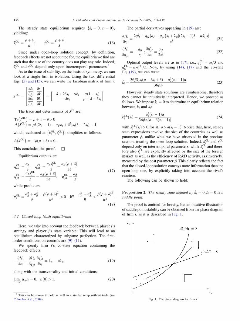
Proposition 2. The steady state defined by ki ¼ 0; si ¼ 0 is a

saddle point.

The proof is omitted for brevity, but an intuitive illustration

of saddle point stability can be obtained from the phase diagram

of firm i; as it is described in Fig. 1.

Fig. 1. The phase diagram for firm i

L. Colombo et al. / Japan and the World Economy 21 (2009) 133–139 137

The stable branch of the saddle is represented by the arrows

pointing at the intersection between loci, from south-west and

north-east of the intersection itself. Some intuitive comparative

statics can be carried out on kCLi sið Þ :

@kCLi sið Þ@a

> 0 ;@kCL

i sið Þ@b

< 0 : (25)

More interesting is the following implication of (24):

@kCLi sið Þ@aJ

> 0 (26)

which tells that

Lemma 3. Given si, the locus of the optimal investment carried

out by either firm shifts upwards with the size of the foreign

market.

We can label this as the foreign market effect: the larger is the

foreign market, the higher is the incentive to carry out R&D

activity to improve the efficiency of transportation, for any given

level of the iceberg cost si. However, we are about to show that, in

equilibrium, any upward shift of the locus ki ¼ 0 brings about a

decrease in the steady state investment, due to the shape of si ¼ 0:

C� 12b rþ dð Þ2 � a2a2J

F� 27b2d3 8b rþ dð Þ3 � a2a2J r� 2dð Þ

h iQ� b3d6 27b 8b rþ dð Þ3 � a2a2

J r� 2dð Þh i2

� 12b rþ dð Þ2 � a2a2J

h i3� �

:

7 There exist other critical points to si ¼ 0; but they can be disregarded as not

real.

The effect of si on kCLi sið Þ can also be characterised:

@kCLi sið Þ@si

¼a2

J rþ d si � 1ð Þ2h i

a

36bs2i r� d si � 1ð Þ½ �2

> 0 ;

which proves the following:

Lemma 4. The locus of the optimal investment in TCRD,

kCLi sið Þ, is upward sloping for all levels of si:

This is due to the fact that, the smaller is the fraction of

exports that can actually reach the foreign market, the higher is

the incentive for firm i to invest in order to improve the

efficiency of the transportation technology.

We are now in a position to derive the implicit profit levels

(for a given level of si) under the closed-loop solution concept.

Before doing this, from a direct comparison between (16) and

(24), it is easy to prove that the optimal effort in TCRD is higher

under the closed-loop than under the open-loop solution (see

Colombo et al., 2004).

This result is in line with the kind of R&D activity at stake,

which aims at increasing the percentage of output that reaches

the foreign market. Moreover, we confirm the conventional

wisdom that firms invest more when using closed-loop

decision rules than open-loop ones (see, e.g., Reynolds,

1987).

The steady state profits accruing to firm i are:

pCLi sið Þ ¼

a2I þ a2

J

9� a4

J si � 1ð Þ2a2

1296bs2i r� d si � 1ð Þ½ �2

(27)

with the relevant property that aI � aJ is sufficient to imply

@pCLi sið Þ=@aI > @pCL

i sið Þ=@aJ ; for any given level of si: That is,

if the home market is at least as large as the foreign one, the

presence of a costly investment to reduce iceberg costs implies

that profits are more sensitive to the home market than to the

foreign market. This quite intuitive feature of the equilibrium

performance of either firm drives us to assess the relative

incentives for firms to invest in TCRD. This is summarised in:

Proposition 5. If aI � aJ then sCLi > sCL

j and kCLi > kCL

j .

Proof. First, we plug kCLi sið Þ into si and impose si ¼ 0; to get7:

sCLi ¼

rþ d

3dþ

3bd2Cþffiffiffiffiffiffiffiffiffiffiffiffiffiffiffiffiffiffiffiffiffiffiffiffiffiffiffiffi

Fþffiffiffiffiffiffiffi3Qp �2

3

r18bd2

ffiffiffiffiffiffiffiffiffiffiffiffiffiffiffiffiffiffiffiffiFþ

ffiffiffiffiffiffiffi3Qp

3p (28)

where:

Now it can be checked that sCLi ¼ sCL

j at aI ¼ aJ ; while

sCLi > sCL

j for all aI > aJ (and conversely). Then, from (5)

and(6), notice that one can write kCLi ¼ dsCL

i =a:Therefore, if

sCLi > sCL

j ; then it must be true that kCLi > kCL

j . &

The above proposition states that, in steady state, the firm

located in the larger country has a comparatively higher

incentive to invest in TCRD than the firm located in the smaller

country. We label this as the home market effect. While the

foreign market effect outlined in Lemma 3 above matters for a

given pair ðsi; s jÞ, the home market effect emerges in steady

state given the equilibrium levels of ðsi; s jÞ, which depends on

ðaJ ; aIÞ: The explanation is the following. Suppose si ¼ s j; if

so, the firm focusses its efforts upon the attempt to improve its

ability to export in terms of how much attractive is the foreign

market, measured by the size of the other country. This is

represented by the fact that kCLi ðsiÞ is a function of aJ but not of

aI . Once the steady state equilibrium is fully characterised,

firms only invest in order to preserve the equilibrium, i.e., the

status quo. In this situation, firm i’s ability to invest so as to

make up for the depreciation rate ultimately depends upon its

capacity to raise revenues to cover the cost of R&D activity.

This is essentially determined by its domestic market, the

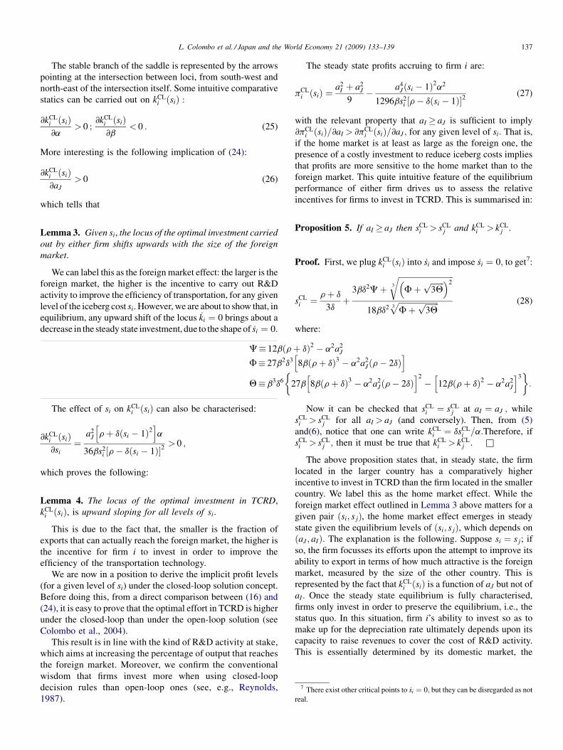
Fig. 2. The phase diagram drawn for aI > aJ

L. Colombo et al. / Japan and the World Economy 21 (2009) 133–139138

intuitive reason being the following. Observing (27), one

immediately notes that the revenues generated by exports

increase with a2J ; while the cost associated with the R&D effort

increases with a4J :Therefore, clearly, the size of the home

market plays a crucial role in allowing firm i to bear the brunt of

R&D expenditure. In this sense, the features of the steady state

equilibrium recall the well known home effect already

highlighted in the existing literature (Helpman and Krugman,

1985; Krugman, 1990). An alternative but equivalent explana-

tion is that the foreign market effect is associated to the pure

incentive to reach foreign consumers, while the home market

effect is associated with covering the cost of making one’s own

exporting technology more efficient.

At this point, it is worth noting that an analogous

investigation made though in a static game framework

(Lambertini and Rossini, 2006) has only highlighted the

existence of a foreign market effect, whereby it is the firm

located in the smaller country that exhibits a higher incentive to

invest at the subgame perfect equilibrium. This seems to

suggest that the dynamic analysis allows one to grasp some

additional features of the issue at hand, as compared to the static

approach.

The foregoing analysis can be described graphically, by

referring to Fig. 2.

In the figure, we assume aI > aJ ; so that the locus ki ¼ 0 lies

everywhere to the right of k j ¼ 0; and below it. Then, note that

a unique locus si ¼ 0 appears, in that the parameters affecting

the state dynamics are fully symmetric across firms. Therefore,

the inequality aI > aJ directly implies both kCLi > kCL

j and

sCLi > sCL

j :

4. Policy implications at the closed-loop equilibrium

The social welfare enjoyed by country I in the steady state

associated with the closed-loop equilibrium is:

SWCLI ¼ pCL

i þ CSCLI (29)

where CSCLI is the instantaneous consumer surplus:

CSCLI ¼

aI � pCLi

� �2

� qCLiI þ

qCLjI

s j

" #¼ 2a2

I

9(30)

and pCLi is given by (27). Therefore, welfare can be written for a

generic si; as follows:

SWCLI sið Þ ¼

a2I

3þ

a2j

9� a4

J si � 1ð Þ2a2

1296bs2i r� d si � 1ð Þ½ �2

We want to investigate the responses of SWCLI ðsiÞ to

different policy measures. Assume that the government of

country I may choose between two kinds of policies: (i) an

R&D subsidy to affect the instantaneous investment costs,

through a reduction of b; (ii) an R&D subsidy affecting the

accumulation process, through an increase of a. Consider, first,

policy (i). Its marginal effect on welfare is given by:

@SWCLI sið Þ@b

¼ a4J si � 1ð Þ2a2

1296b2s2i r� d si � 1ð Þ½ �2

> 0 (31)

Therefore, a marginal increase in b improves welfare. This

can be explained as follows. An increase in b reduces kCLi ðsiÞ;

as we know from (25). This suggests that firms invest too much

in R&D as compared to what would be socially optimal, given

the output levels chosen on the basis of profit maximisation.

As to policy (ii), its effect is given by:

@SWCLI sið Þ@a

¼ � a4J si � 1ð Þ2a

648bs2i r� d si � 1ð Þ½ �2

< 0 (32)

Likewise, a marginal decrease in a yields a welfare

improvement, since it slows down the R&D investment.

In line of principle, the two measures could obviously be

implemented together. However, this may not be possible. In

order to understand which one should be preferred, we consider

the following:

@WCLI ðsiÞ@a

�������� ¼ 2b

a

@WCLI ðsiÞ@b

�������� (33)

It is immediate to draw from it:

Proposition 6. For all b>a=2, it is preferable to reduce the

investment efforts of firms by reducing the productive efficiency

of R&D activity, rather than increasing the cost of R&D

investment, and vice versa.

That is, a welfare-improving reduction of excess investment

typically emerging in Cournot markets (as in Brander and

Spencer, 1983; Spencer and Brander, 1983), can be attained

through several forms of taxation, affecting either the perceived

cost of R&D activity to be accounted for in instantaneous

profits (parameter b), or the performance of R&D activity itself

(parameter a).

L. Colombo et al. / Japan and the World Economy 21 (2009) 133–139 139

5. Concluding remarks

We have analysed a dynamic Cournot duopoly with

intraindustry trade, where firms invest so as to reduce the

level of iceberg transportation costs. We have derived both

open-loop and closed-loop equilibria, showing that a unique

(saddle point) steady state exists in both cases. In the open-loop

model, optimal investments and the resulting efficiency of

transportation technology are independent of the relative size of

the two countries. On the contrary, in the closed-loop case, a

foreign market effect drives firms’ investments for any given

level of iceberg costs, while a home market effect operates in

the long run equilibrium only, so that the firm located in the

larger country invests more than the rival located in the smaller

one.

In order to reduce the excessive amount of R&D effort by the

domestic firm, a policy maker aiming at enhancing domestic

social welfare may adopt two different types of R&D taxation,

or a mix thereof.

Acknowledgements

We thank Giacomo Calzolari, Paul Walsh, an anonymous

referee and the audience at Trinity College Dublin and the

University of Nottingham for useful comments and discussion.

References

Anderson, J.E., Marcouiller, D., 1999. Trade, insecurity, and home bias. An

empirical investigation. NBER working paper no. 7000.

Brander, J., 1981. Intra-industry trade in identical commodities. Journal of

International Economics 11, 1–14.

Brander, J., Spencer, B., 1983. Strategic commitment with R&D: the symmetric

case. Bell Journal of Economics 14, 225–235.

Calzolari, G., Lambertini, L., 2006. Tariffs vs. quotas in a trade model with

capital accumulation. Review of International Economics 14, 632–644.

Calzolari, G., Lambertini, L. 2007. Export restraints in a model of trade with

capital accumulation. Journal of Economic Dynamics and Control. 31,

3822–3842.

Cellini, R., Lambertini, L., 2003. Differential oligopoly games. In: Bianchi,

P., Lambertini, L. (Eds.), Technology, Information and Market

Dynamics: Topics in Advanced Industrial Organization. Edward Elgar,

London, pp. 173–207.

Colombo, L., Lambertini, L., Mantovani, A., 2004. A differential game with

investments in transport and communication R&D. International Journal of

Mathematics, Game Theory, and Algebra 14, 363–374 (also published in

Petrosjan, L., Mazalov, V. (Eds.), 2005. Game Theory and Applications, vol.

X. Nova Science Publisher, New York.

Dockner, E.J., Jorgensen, S., Long, N.V., Sorger, G., 2000. Differential Games

in Economics and Management Science. Cambridge University Press,

Cambridge.

Harley, C., 1980. Transportation the world wheat trade and the Kuznets cycle

1850–1993. Explorations in Economic History 17, 218–250.

Helpman, E., Krugman, P., 1985. Market Structure and Foreign Trade. MIT

Press, Cambridge, MA.

Krugman, P., 1990. Rethinking International Trade. MIT Press, Cambridge,

MA.

Lambertini, L., Rossini, G., 2006. Investment in transport and communication

technology in a Cournot duopoly with trade. Japan and the World Economy

18, 221–229.

McCallum, J., 1996. National borders matter: Canada–US regional trade

patterns. American Economic Review 85, 615–623.

Obstfeld, M., Rogoff, K., 2000. The six major puzzles in international

macroeconomics: is there a common cause? NBER working paper no.

7777.

O’Rourke, K.H., Williamson, J.G., 1999. Globalization and History. The

Evolution of the Nineteenth Century Atlantic Economy. MIT Press, Cam-

bridge, MA.

Reynolds, S.S., 1987. Capacity investment, preemption and commitment in an

infinite horizon model. International Economic Review 28, 69–88.

Samuelson, P., 1954. The transfer problem and transport costs II: analysis of

effects of trade impediments. Economic Journal 64, 264–289.

Singh, N., Vives, X., 1984. Price and quantity competition in a differentiated

duopoly. RAND Journal of Economics 15, 546–554

Spencer, B.J., Brander, J.A., 1983. International R&D rivalry and industrial

strategy. Review of Economic Studies 50, 707–722.

Turrini, A., van Ypersele, T., 2002. Traders, courts and the home bias puzzle.

CEPR discussion paper no. 3228.