FEDERAL RESERVE BANK OF SAN FRANCISCO

WORKING PAPER SERIES

Endogenous Regime Switching Near the Zero Lower Bound

Kevin J. Lansing Federal Reserve Bank of San Francisco

February 2018

Working Paper 2017-24 http://www.frbsf.org/economic-research/publications/working-papers/2017/24/

Suggested citation:

Kevin J. Lansing. 2017. “Endogenous Regime Switching Near the Zero Lower Bound” Federal Reserve Bank of San Francisco Working Paper 2017-24. https://doi.org/10.24148/wp2017-24 The views in this paper are solely the responsibility of the authors and should not be interpreted as reflecting the views of the Federal Reserve Bank of San Francisco or the Board of Governors of the Federal Reserve System.

Endogenous Regime Switching Near the Zero Lower Bound∗

Kevin J. Lansing†

Federal Reserve Bank of San Francisco

February 23, 2018

Abstract

This paper develops a New Keynesian model with a time-varying natural rate of inter-est (r-star) and a zero lower bound (ZLB) on the nominal interest rate. The representa-tive agent contemplates the possibility of an occasionally binding ZLB that is driven byswitching between two local equilibria, labeled the “targeted”and “deflation”regimes, re-spectively. Sustained periods when the real interest rate remains below the central bank’sestimate of r-star can induce the agent to place a substantially higher weight on the defla-tion forecast rules, causing the deflation equilibrium to occasionally become fully realized.I solve for the time series of stochastic shocks and endogenous forecast rule weights thatallow the model to exactly replicate the observed time paths of the U.S. output gap, quar-terly inflation, and the federal funds rate since 1988. The data since the start of the ZLBepisode in 2008.Q4 are best described as a mixture of the two local equilibria. In modelsimulations, raising the central bank’s inflation target to 4% from 2% can reduce, but noteliminate, the endogenous switches to the deflation equilibrium.

Keywords: Natural rate of interest, New Keynesian, Liquidity trap, Zero lower bound,Taylor rule, Deflation.

JEL Classification: E31, E43, E52.

∗An earlier version of this paper was titled “Endogenous Regime Shifts in a New Keynesian Model with aTime-Varying Natural Rate of Interest.”The views in this paper are my own and not necessarily those of theFederal Reserve Bank of San Francisco or the Board of Governors of the Federal Reserve System. For helpfulcomments and suggestions, I thank James Bullard, Gavin Goy, Giovanni Ricco, Stephanie Schmitt-Grohé,Roman Šustek, FRBSF and Norges Bank colleagues, and session participants at the 2017 AEA Meeting, the2017 SNDE Symposium, the 2017 Monash University Macro-Finance Workshop, the 2017 Bank of Englandconference on “Applications of Behavioral Economics and Multiple Equilibria to Macroeconomic Policy,” the2017 Conference on “Expectations in Dynamic Macroeconomic Models,”hosted by the Federal Reserve Bankof St. Louis, the 2017 Vienna Macroeconomics Workshop, and the 2018 Norges Bank Conference on “NonlinearModels in Macroeconomics and Finance.”†Federal Reserve Bank of San Francisco, P.O. Box 7702, San Francisco, CA 94120-7702, email:

kevin.j.lansing@sf.frb.org

1 Introduction

The sample period from 1988 onwards is generally viewed as an example of consistent U.S.

monetary policy aimed at keeping inflation low while promoting sustainable growth and full

employment. Amazingly, the U.S. federal funds rate has been pinned close to zero for about

one-fourth of the elapsed time since 1988. The U.S. economy is not alone in experiencing an

extended period of zero or mildly negative nominal interest rates in recent decades.

Figure 1 plots three-month nominal Treasury bill yields in the United States, Japan,

Switzerland, and the United Kingdom. Nominal interest rates in the United States encoun-

tered the zero lower bound during the 1930s and from 2008.Q4 though 2015.Q4. Nominal

interest rates in Japan have remained near zero since 1998.Q3, except for the relatively brief

period from 2006.Q4 to 2008.Q3. Nominal interest rates in Switzerland have been zero or

slightly negative since 2008.Q4. Nominal interest rates in the United Kingdom have been ap-

proximately zero since 2009.Q1. Outside of these episodes, all four countries exhibit a strong

positive correlation between nominal interest rates and inflation, consistent with the Fisher

relationship.

Benhabib, Schmitt-Grohé and Uribe (2001a,b) show that imposing a zero lower bound

(ZLB) on the nominal interest rate in a standard New Keynesian model gives rise to two

long-run endpoints (steady states).1 The basic idea is illustrated in Figure 2, which is adapted

from Bullard (2010). The two intersections of the ZLB-augmented monetary policy rule (solid

red line) with the Fisher relationship (dashed black line) define two long-run endpoints. I refer

to these as the “targeted equilibrium”and “deflation equilibrium,” respectively. The aim of

this paper is to develop a quantitative New Keynesian model that can account for the pattern

of inflation and interest rates observed in Figure 2 since 1988.

The model incorporates three types of persistent shocks: an aggregate demand shock, a

cost push shock, and a shock to the agent’s discount factor that gives rise to movements in the

real short-term interest rate. The long-run endpoint of the real interest rate process is allowed

to shift over time. This feature captures the notion of a time-varying natural rate of interest

(r-star). R-star is an important benchmark for monetary policy because it determines the real

interest rate that policymakers should aim for once shocks to the economy have dissipated

and the central bank’s macroeconomic targets have been achieved.2 The times series process

1 I use the terminology “long-run endpoints”rather than “steady states”because the model developed hereallows for permanent shifts in the natural rate of interest which, in turn, can shift the long-run values of somemacroeconomic variables.

2Willamson (2017a) provides a discussion of the distinctions between the “natural,” “equilibrium,” and

1

for r-star in the model is calibrated to approximate the path of the U.S. natural rate series

estimated by Laubach and Williams (2016).3

As is well known, the New Keynesian deflation equilibrium is locally indeterminate. I

therefore consider a minimum state variable (MSV) solution that rules out sunspot variables

and extra lags of fundamental state variables. The decision rules associated with the deflation

equilibrium induce more volatility in the output gap and inflation in response to real interest

rate shocks. Model variables in the deflation equilibrium have distributions with lower means

and higher variances than those in the targeted equilibrium. But the significant overlap in

the various distributions creates a dilemma for an agent who seeks to determine the likelihood

that a string of recent data observations are drawn from one equilibrium or the other.

The representative agent in the model contemplates the possibility of an occasionally bind-

ing ZLB that is driven by switching between the two local equilibria. This view turns out to

be true in the simulations, thus validating the agent’s beliefs. The agent constructs forecasts

using a form of model averaging, where the time-varying forecast weights are determined by

recent performance, as measured by the root mean squared forecast errors for the output gap

and inflation (the two variables that the agent must forecast). Sustained periods when the

exogenous real interest rate remains below the central bank’s estimate of r-star can induce

the agent to place a substantially higher weight on the deflation forecast rules, causing the

deflation equilibrium to occasionally become fully realized. These episodes are accompanied

by highly negative output gaps and a binding ZLB, reminiscent of the U.S. Great Recession.

But even outside of recessions or when the ZLB is not binding, the agent may continue to

assign a nontrivial weight to the deflation equilibrium, causing the central bank to persistently

undershoot its inflation target, similar to the U.S. economy since mid-2012.

I solve for the time series of stochastic shocks and endogenous forecast rule weights that

allow the switching model to exactly replicate the observed time paths of the CBO output

gap, quarterly PCE inflation, and the federal funds rate since 1988. The data since the start

of the ZLB episode in 2008.Q4 are best described as a mixture of the two local equilibria. The

model-implied weight on the targeted forecast rules starts to decline in 2008.Q4. At the end

of the data sample in 2017.Q2, the weight on the targeted forecast rules is only 0.56, helping

the switching model to account for the persistent undershooting of the Fed’s inflation target

since mid-2012. The path of expected inflation from the switching model starts to decline

after 2008.Q4 and remains below the Fed’s 2% inflation target at the end of the data sample.

“neutral”real rates of interest– terms that are often used interchangeably in the literature.3Updated data are from www.frbsf.org/economic-research/files/Laubach_Williams_updated_estimates.xlsx.

2

This pattern is very similar to the 1-year expected inflation rate from inflation swap contracts.

The framework developed here is related to work by Aruoba and Schorfheide (2016) and

Aruoba, Cuba-Borda, and Schorfheide (2018). These authors construct stochastic two-regime

models in which the economy can switch back and forth between a targeted-inflation regime

and a deflation regime, depending on the realization of an exogenous sunspot variable. They

employ various model specifications to infer whether the interest rate and inflation observations

in the data are more likely to have been generated by one regime or the other. Aruoba, Cuba-

Borda, and Schorfheide (2018, p. 116) conclude that “the U.S. remained in the targeted-

inflation regime during its ZLB episode, with the possible exception of the early part of 2009

where evidence is ambiguous.”

An important premise underlying the results of Aruoba, Cuba-Borda, and Schorfheide

(2018) is that the observed data must come from one regime or the other. In contrast, the

switching model developed here generates data that is a convex mixture of the two regimes.

This is due to the time-varying forecasts weights assigned by the agent in the model. The

forecast weights, in turn, influence the model-generated data. So, the deflation regime can

influence the model-generated data even if the deflation equilibrium is never fully realized.

Another key difference is that the probability of transitioning between regimes is endogenous

here, and can be influenced by a change in the monetary policy rule or other model parame-

ters. The switching model shares some similarities with the work of Sargent (1999) in which

the economy can endogenously transition between regimes of high versus low inflation, de-

pending on policymakers’perceptions about the slope of the long-run Phillips curve. Here,

the endogenous regime switching depends on the agent’s perceptions about the best forecast

weights.

Another related paper is one by Dordal-i-Carrera et al. (2016). These authors develop

a New Keynesian model with volatile and persistent “risk shocks” (i.e., shocks that drive a

wedge between the nominal policy rate and the short-term bond rate) to account for infrequent

but long-lived ZLB episodes. A risk shock in their model is isomorphic to a real interest rate

shock here. Large adverse risk shocks are themselves infrequent and long-lived. As the binding

ZLB episode becomes more frequent or more long-lived, the optimal inflation target increases.

Unlike here, their analysis does not consider model solutions near the deflation equilibrium, but

rather focuses on scenarios in which fundamental shocks are large enough to push the targeted

equilibrium to a point where ZLB becomes binding.4 In contrast, the model developed here

4This is also the methodology pursued by Reifschneider and Williams (2000), Schmitt-Grohé and Uribe

3

accounts for infrequent but long-lived ZLB episodes via endogenous switching between two

local equilibria, i.e., the shock process itself is not the sole driving force for the infrequent and

long-lived ZLB episodes.

As part of the quantitative analysis, I examine how raising the central bank’s inflation

target can influence the ZLB binding frequency and the volatility of macro variables in the

switching model. I find that even with an inflation target of 4%, the ZLB binding frequency

remains elevated at 9.5% and the average duration of a ZLB episode is 11.7 quarters. Once

the deflation equilibrium is taken into account, raising the inflation target is a less effective

solution for avoiding ZLB episodes.

Numerous papers consider optimal monetary policy in response to a time-varying natural

rate of interest. The models typically impose the ZLB (or effective lower bound), but the

deflation equilibrium is ignored, i.e., the analysis is local to the targeted equilibrium.5 One

finding from literature is that more uncertainty about the future natural rate implies looser

monetary policy today or more policy inertia. Here I show that more policy inertia (i.e., a

larger interest rate smoothing parameter in the Taylor-type rule) serves to decrease the ZLB

binding frequency, but the episodes exhibit longer duration on average.

It has been suggested by some that the deflation equilibrium should be ignored because

it may not be learnable using standard algorithms. A typical conclusion from the literature

is that only the targeted equilibrium is locally (but not globally) stable under least squares

learning.6 Recently, however, Arifovic, Schmitt-Grohé, and Uribe (2018) demonstrate that

both equilibria can be locally stable under a form of social learning. In the last section of the

paper, I introduce an adaptive learning algorithm in a simplified version of the model. When

the agent estimates correctly specified decision rules, the algorithm quickly converges to the

vicinity of the targeted equilibrium and remains there. But when the agent estimates decision

rules that fail to control for two white noise shocks, the model exhibits low frequency switching

between the two local equilibria. This pattern is qualitatively similar to that observed in the

original switching model with full-knowledge.

(2010), Chung et al. (2012), Coibion, Gorodnichenko, and Wieland (2012), Dennis (2016), and Kiley andRoberts (2017).

5See, for example, Eggertsson and Woodford (2003), Adam and Billi (2007), Nakov (2008), Nakata (2013),Hamilton, et al. (2016), Basu and Bundick (2015), Evans, et al. (2015), and Gust, Johannsen, López-Salido(2017).

6See, for example, Evans and Honkapohja 2005, Eusepi 2007, Evans, Guse, and Honkapohja 2008, Benhabib,Evans and Honkapohja 2014, and Christiano, Eichenbaum, and Johanssen 2016.

4

2 Model

The framework for the analysis is a three equation New Keynesian model, augmented by a zero

lower bound on the short-term nominal interest rate. The log-linear version of the standard

New Keynesian model is taken to represent a set of global equilibrium conditions, with the

only nonlinearity coming from the ZLB. The setup is a reduced form version of a fully-specified

nonlinear New Keynesian DSGE model, but has the advantage of delivering transparency of

the model’s dynamics.7

Private-sector behavior is governed by the following equilibrium conditions:

yt = Et yt+1 − α[it − Et πt+1 − rt] + νt, (1)

πt = βEt πt+1 + κyt + ut, (2)

where equation (1) is the representative agents’s consumption Euler equation and equation

(2) is the Phillips curve that is derived from the representative firm’s optimal pricing decision.

The variable yt is the output gap (the log deviation of real output from potential output), πt

is the quarterly inflation rate (log difference of the price level), it is the short-term nominal

interest rate, rt is the exogenous real interest rate, and Et is the expectations operator. In

solving the model, Et will correspond to rational expectations in the vicinity of the model’s

long-run endpoints. Fluctuations in rt can be interpreted as arising from changes in the agent’s

rate of time preference or changes in the expected growth rate of potential output.8 None of

the results in the paper are sensitive to the introduction of a discount factor applied to the

term Et yt+1 in equation (1), along the lines of McKay, Nakamura, and Steinsson (2016). The

terms νt and ut represent an aggregate demand shock and a cost-push shock, respectively,

which evolve according to following laws of motion:

νt = ρννt−1 + εν,t, εν,t ∼ N[0, σ2ν

(1− ρ2ν

)], (3)

ut = ρuut−1 + εu,t, εu,t ∼ N[0, σ2u

(1− ρ2u

)]. (4)

The time series process for the exogenous real rate of interest is given by

rt = ρr rt−1 + (1− ρr) r∗t + εt, εt ∼ N(0, σ2ε

), (5)

r∗t = r∗t−1 + ηt, ηt ∼ N(0, σ2η

). (6)

7Armenter (2016) adopts a similar approach in computing the optimal monetary policy in the presence oftwo steady states. Eggertsson and Sing (2016) show that the log-linear New Keynesian model behaves verysimilar to the true nonlinear model in the vicinity of the targeted equilibrium.

8Specifically, we have rt ≡ − log [β exp (ζt)] + γEt∆yt+1, where ζt is a shock to the agent’s time discountfactor β, yt is the logarithm of real potential output, and γ = α−1 is the coeffi cient of relative risk aversion.For the derivation, see Hamilton, et al. (2016) or Gust, Johannsen, and Lopez-Salido (2017).

5

Equations (5) and (6) summarize a “shifting endpoint”time series process since the long-run

endpoint r∗t can vary over time due to the permanent shock ηt. In any given period, rt can

deviate from r∗t due to the temporary shock εt. The persistence of the “real interest rate gap”

rt − r∗t is governed by the parameter ρr, where |ρr| < 1. Kozicki and Tinsely (2012) employ

this type of process to describe U.S. inflation. When ρr = 1, we recover the random walk plus

noise specification employed by Stock and Watson (2007) to describe U.S. inflation.9

Using equation (5) to substitute out rt from equation (1) yields the following alternative

version of the consumption Euler equation:

yt = Et yt+1 − α[it − Et πt+1 − r∗t ] + ut + αεt + αρr(rt−1 − r∗t−1 − ηt

), (7)

where the last three terms could be consolidated into a single aggregate demand shock. From

this version, we can interpret r∗t as the unobservable “natural rate of interest,” i.e., the real

interest rate that is consistent with full utilization of economic resources and steady inflation

at the central bank’s target rate. This interpretation is consistent with the empirical strategies

of Laubach and Williams (2016), Lubik and Matthes (2015), and Kiley (2015) which view the

natural rate of interest as a longer-term economic concept. In contrast, empirical strategies

that employ micro-founded New Keynesian models typically view the natural (or equilibrium)

rate of interest as a short-term concept, more along the lines of the variable rt in equation

(1).10 The real interest rate gap rt − r∗t captures a concept that has been emphasized by Fedpolicymakers in recent speeches, namely, a distinction between estimates of the “short-term

natural of interest” and its longer-term counterpart (Yellen 2015, Dudley 2015, and Fischer

2016). Here I will refer to r∗t as the natural rate of interest.

In the model, the agent’s rational forecast for the real interest rate gap at any horizon

h ≥ 1 is given by

Et(rt+h − r∗t+h

)= (ρr)

h (rt − Etr∗t ) , (8)

where Etr∗t represents the current estimate of the natural rate computed using the Kalman

filter so as to minimize the mean squared forecast error. When |ρr| < 1 as assumed here,

the real interest rate gap is expected to shrink to zero as the forecast horizon h increases. In

9But unlike here, Stock and Watson (2007) allow for stochastic volatility in the permanent and temporaryshocks.10See, for example, Barsky, Justiniano, and Melosi (2014), Cúrdia, et al. (2015), and Del Negro, et al. (2017).

6

Appendix A, I show that the Kalman filter expression for Etr∗t is

Etr∗t = λ

[rt − ρr rt−1

1− ρr

]+ (1− λ) Et−1r

∗t−1 (9)

λ =− (1− ρr)2 φ+ (1− ρr)

√(1− ρr)2 φ2 + 4φ

2, (10)

where λ is the Kalman gain parameter and φ ≡ σ2η/σ2ε. For the quantitative analysis, the valuesof ρr, σ

2η, and σ

2ε are chosen so that the time path of Etr

∗t from equation (9) approximates the

path of the U.S. natural rate series estimated by Laubach and Williams (2016, updated) for the

sample period 1988.Q1 to 2017.Q2. Their estimation strategy assumes that the natural rate

exhibits a unit root, consistent with equation (6). Hamilton, et al. (2016) present evidence

that the ex-ante real rate of interest it − Et πt+1 in U.S. data is nonstationary, but they findthat the gap between the ex-ante real rate and their estimate of the world long-run real rate

appears to be stationary. This evidence is also consistent with equations (5) and (6) which

imply that real rate gap rt − r∗t is stationary.The central bank’s monetary policy rule is given by

i∗t = ρi∗t−1 + (1− ρ) [Etr∗t + π∗ + gπ (πt − π∗) + gy (yt − y∗)] , (11)

πt = ω πt + (1− ω) πt−1, (12)

it = max {0, i∗t } , (13)

where i∗t is the desired nominal interest rate that responds to deviations of recent inflation πt

from the central bank’s target rate π∗ and to deviations of the output gap from its targeted

long-run endpoint y∗. Recent inflation πt is an exponentially-weighted moving average of past

quarterly inflation rates so as to approximate the compound average inflation rate over the

past 4 quarters– a typical central bank target variable.11 Equation (13) is the ZLB that

constrains the nominal policy interest rate it to be non-negative. The parameter ρ governs the

degree of interest rate smoothing as i∗t adjusts partially each period toward the value implied

by the terms in square brackets. Similar to the policy rule employed by Dordal-i-Carrera et

al. (2016), equation (11) keeps track of past negative values of i∗t , thereby exhibiting a form of

commitment to keep interest rates “lower for longer”whenever the ZLB becomes binding.12

The quantity Etr∗t + π∗ represents the targeted long-run endpoint of i∗t . Including Etr∗t in

the policy rule implies that monetary policymakers continually update their estimate of the11Specifically, the value of ω is set to achieve πt ' [Π3

j=0(1 + πt−j)]0.25 − 1

12Alstadheim and Henderson (2006) and Sugo and Ueda (2008) formulate interest rate rules that can precludethe deflation equilibrium.

7

unobservable r∗t . Support for this idea can be found in the Federal Open Market Committee’s

Summary of Economic Projections (SEP). Meeting participants provide their views on the

projected paths of macroeconomic variables over the next three calendar years and in the

longer run. Since the natural rate of interest is a longer-run concept, we can infer the median

SEP projection for r∗t by subtracting the median longer-run projection for inflation from the

median longer-run projection for the nominal federal funds rate. The median SEP projection

for r∗t computed in this way has ratcheted down over time, as documented by Lansing (2016).13

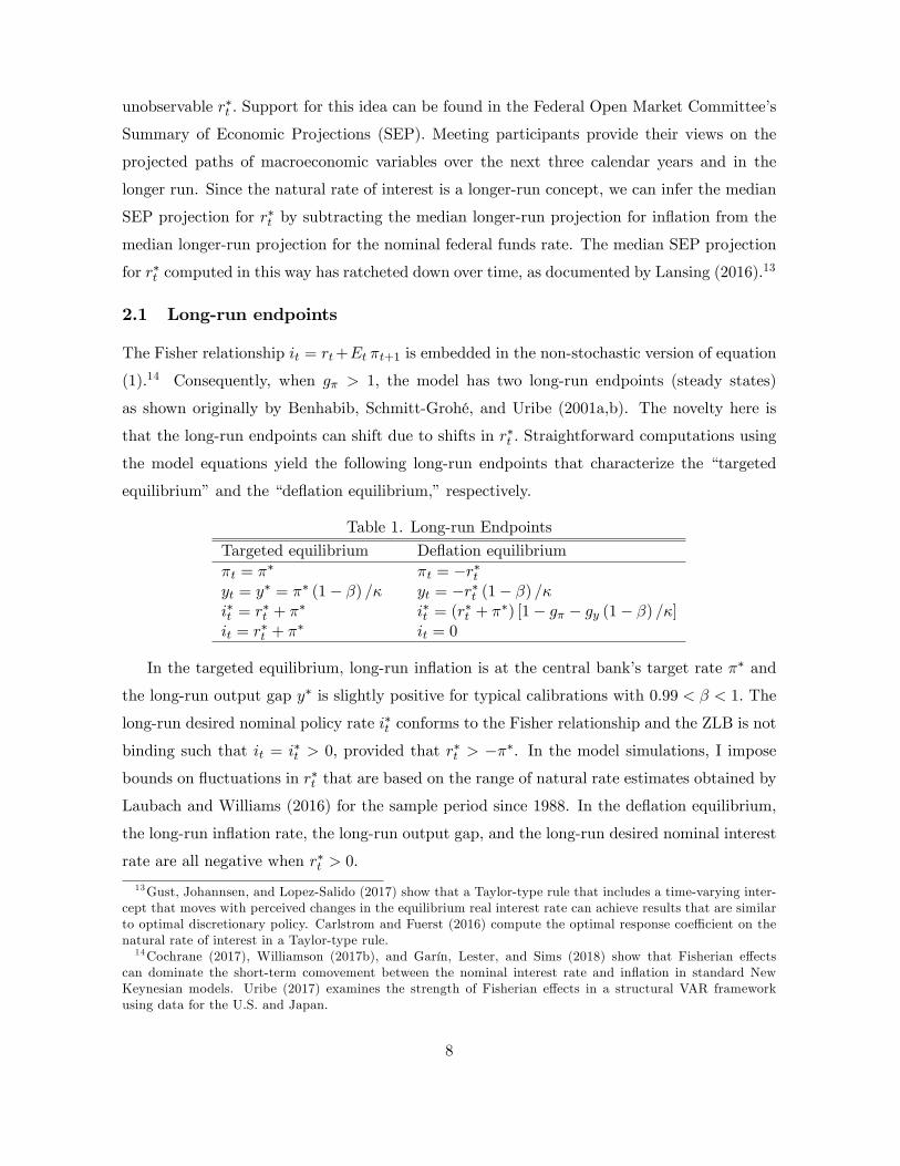
2.1 Long-run endpoints

The Fisher relationship it = rt+Et πt+1 is embedded in the non-stochastic version of equation

(1).14 Consequently, when gπ > 1, the model has two long-run endpoints (steady states)

as shown originally by Benhabib, Schmitt-Grohé, and Uribe (2001a,b). The novelty here is

that the long-run endpoints can shift due to shifts in r∗t . Straightforward computations using

the model equations yield the following long-run endpoints that characterize the “targeted

equilibrium”and the “deflation equilibrium,”respectively.

Table 1. Long-run Endpoints

Targeted equilibrium Deflation equilibriumπt = π∗ πt = −r∗tyt = y∗ = π∗ (1− β) /κ yt = −r∗t (1− β) /κi∗t = r∗t + π∗ i∗t = (r∗t + π∗) [1− gπ − gy (1− β) /κ]it = r∗t + π∗ it = 0

In the targeted equilibrium, long-run inflation is at the central bank’s target rate π∗ and

the long-run output gap y∗ is slightly positive for typical calibrations with 0.99 < β < 1. The

long-run desired nominal policy rate i∗t conforms to the Fisher relationship and the ZLB is not

binding such that it = i∗t > 0, provided that r∗t > −π∗. In the model simulations, I imposebounds on fluctuations in r∗t that are based on the range of natural rate estimates obtained by

Laubach and Williams (2016) for the sample period since 1988. In the deflation equilibrium,

the long-run inflation rate, the long-run output gap, and the long-run desired nominal interest

rate are all negative when r∗t > 0.

13Gust, Johannsen, and Lopez-Salido (2017) show that a Taylor-type rule that includes a time-varying inter-cept that moves with perceived changes in the equilibrium real interest rate can achieve results that are similarto optimal discretionary policy. Carlstrom and Fuerst (2016) compute the optimal response coeffi cient on thenatural rate of interest in a Taylor-type rule.14Cochrane (2017), Williamson (2017b), and Garín, Lester, and Sims (2018) show that Fisherian effects

can dominate the short-term comovement between the nominal interest rate and inflation in standard NewKeynesian models. Uribe (2017) examines the strength of Fisherian effects in a structural VAR frameworkusing data for the U.S. and Japan.

8

2.2 Local linear forecast rules

Given the linearity of the model aside from the ZLB, it is straightforward to derive the agent’s

rational decision rules for yt and πt in the vicinity of the long-run endpoints associated with

each of the two equilibria. For the targeted equilibrium, the local decision rules are unique

linear functions of the state variables: rt, Etr∗t , πt−1, i∗t−1, νt, and ut. For the deflation equilib-

rium, I solve for the minimum state variable (MSV) solution which abstracts from extraneous

sunspot variables and extra lags of fundamental state variables.15

Given the local linear decision rules, we can construct the agent’s local linear forecast rules

for yt+1 and πt+1 in each of the two equilibria. As shown in Appendices B and C, the local

linear forecast rules depend on the realizations of πt and i∗t . But since πt and i∗t depend in

part on the agent’s forecasts, there exists simultaneity between the forecasted and realized

values of πt and i∗t . To handle this simultaneity in the numerical simulations, I substitute the

local linear forecast rules into the global equilibrium conditions (1) and (2). I allow for an

occasionally binding ZLB by making the substitution it = 0.5 i∗t + 0.5√

(i∗t )2 in equation (1).

Together with the monetary policy rule (11), this procedure yields a system of three equations

that can be solved each period to obtain the three realizations yt, πt, and i∗t .

The decision rule coeffi cients applied to the state variable rt − Etr∗t are much larger inmagnitude in the deflation equilibrium than in the targeted equilibrium (see Appendices B

and C). Consequently, the deflation equilibrium exhibits more volatility and undergoes a more

severe recession in response to an adverse shock sequence that causes rt−Etr∗t to be persistentlynegative. The higher volatility in the deflation equilibrium is due to the binding ZLB which

prevents the central bank from taking action to mitigate the consequences of the adverse shock

sequence.

The local linear forecast rules for the targeted equilibrium are derived under the assumption

that i∗t > 0 and hence do not take into account the possibility that a shock sequence could be

large enough to cause the ZLB to become binding in the future. The error induced by the use of

linear forecast rules will depend on the frequency and duration of ZLB episodes in the targeted

equilibrium. Based on model simulations, the targeted equilibrium experiences a binding ZLB

in only 2.5% of the periods, with an average duration of 5.3 quarters. The local linear forecast

rules for the deflation equilibrium are derived under the assumption that i∗t ≤ 0 and hence

do not take into account the possibility that a shock sequence could be large enough to cause

the ZLB to become slack in the future. Based on model simulations, the deflation equilibrium

15For background on MSV solutions, see McCallum (1999).

9

experiences a binding ZLB in 80% of the periods, with an average duration of 35 quarters.

The average duration of a slack ZLB episode in the deflation equilibrium is 8.5 quarters. The

It is important to recognize, however, that the agent in the switching model (described below)

does not encounter these particular statistics because they pertain to environments with no

regime switching. In Section 4, I show that the agent’s forecast errors in the switching model

are close to white noise.

Aruoba, Cuba-Borda, and Schorfheide (2018) solve for piece-wise linear decision rules to

account for the occasionally binding nature of the ZLB constraint within each of the two

regimes of their model. They report (p. 104), that the probability of hitting the ZLB in the

targeted-inflation regime is “virtually zero”given the pre-crisis distribution of shocks. In the

deflation regime, the probability of hitting the ZLB is 89%. These statistics are similar to

those obtained here using the linear forecast rules.

Focusing only on the targeted equilibrium, Richter and Throckmorton (2016) compare a

linear model solution in which agents’forecasts do not account for the possibility of hitting

the ZLB (but the ZLB is imposed in simulations, as done here) to a nonlinear model solution

in which agents’ forecasts do account for this possibility. They report that the posterior

distributions and marginal likelihoods of the two models are similar. But the nonlinear model

predicts higher output volatility and more-negative skewness in output and inflation during

the ZLB episode.

2.3 Endogenous regime switching

I now consider an agent who contemplates the possibility of an occasionally binding ZLB

that is driven by switching between the two local equilibria, which can be viewed as two

separate regimes. This setup bears some resemblance to the “OccBin toolkit”solution method

developed by Guerrieri and Iacoviello (2015). Despite taking into account the possibility of

occasionally hitting the ZLB, the agent’s use of linear forecast rules within each regime is fully

rational only in a vicinity of the model’s long-run endpoints.

From the agent’s perspective, one set of local linear forecast rules might perform better than

the other depending on the realizations of the macroeconomic variables over a given sample

period. The agent constructs forecasts using a form of model averaging– a technique that is

often employed to improve forecast performance in situations where the true data generating

process (or true regime) is unknown (Timmerman 2006). The agent in the switching model can

be viewed as an econometrician trying to identify the best forecast rule for the environment.

10

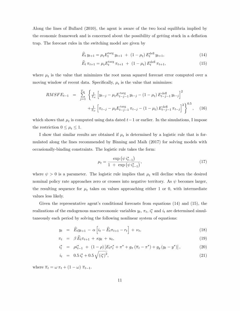
Along the lines of Bullard (2010), the agent is aware of the two local equilibria implied by

the economic framework and is concerned about the possibility of getting stuck in a deflation

trap. The forecast rules in the switching model are given by

Et yt+1 = µtEtargt yt+1 + (1− µt)Edeflt yt+1, (14)

Et πt+1 = µtEtargt πt+1 + (1− µt)Edeflt πt+1, (15)

where µt is the value that minimizes the root mean squared forecast error computed over a

moving window of recent data. Specifically, µt is the value that minimizes:

RMSFEt−1 =Tw∑j=1

{1Tw

[yt−j − µtE

targt−j−1 yt−j − (1− µt)E defl

t−j−1 yt−j]2

+ 1Tw

[πt−j − µtE

targt−j−1 πt−j − (1− µt)E defl

t−j−1 πt−j]2}0.5

, (16)

which shows that µt is computed using data dated t−1 or earlier. In the simulations, I impose

the restriction 0 ≤ µt ≤ 1.

I show that similar results are obtained if µt is determined by a logistic rule that is for-

mulated along the lines recommended by Binning and Maih (2017) for solving models with

occasionally-binding constraints. The logistic rule takes the form:

µt =exp

(ψ i∗t−1

)1 + exp

(ψ i∗t−1

) , (17)

where ψ > 0 is a parameter. The logistic rule implies that µt will decline when the desired

nominal policy rate approaches zero or crosses into negative territory. As ψ becomes larger,

the resulting sequence for µt takes on values approaching either 1 or 0, with intermediate

values less likely.

Given the representative agent’s conditional forecasts from equations (14) and (15), the

realizations of the endogenous macroeconomic variables yt, πt, i∗t and it are determined simul-

taneously each period by solving the following nonlinear system of equations:

yt = Etyt+1 − α[it − Etπt+1 − rt

]+ νt, (18)

πt = β Etπt+1 + κyt + ut, (19)

i∗t = ρi∗t−1 + (1− ρ) [Etr∗t + π∗ + gπ (πt − π∗) + gy (yt − y∗)] , (20)

it = 0.5 i∗t + 0.5

√(i∗t )

2, (21)

where πt = ω πt + (1− ω) πt−1.

11

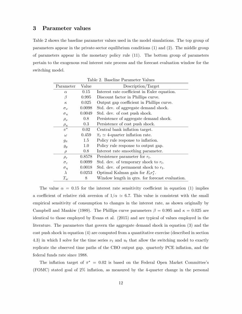
3 Parameter values

Table 2 shows the baseline parameter values used in the model simulations. The top group of

parameters appear in the private-sector equilibrium conditions (1) and (2). The middle group

of parameters appear in the monetary policy rule (11). The bottom group of parameters

pertain to the exogenous real interest rate process and the forecast evaluation window for the

switching model.

Table 2. Baseline Parameter Values

Parameter Value Description/Targetα 0.15 Interest rate coeffi cient in Euler equation.β 0.995 Discount factor in Phillips curve.κ 0.025 Output gap coeffi cient in Phillips curve.σν 0.0098 Std. dev. of aggregate demand shock.σu 0.0049 Std. dev. of cost push shock.ρν 0.8 Persistence of aggregate demand shock.ρu 0.3 Persistence of cost push shock.π∗ 0.02 Central bank inflation target.ω 0.459 πt ' 4-quarter inflation rate.gπ 1.5 Policy rule response to inflation.gy 1.0 Policy rule response to output gap.ρ 0.8 Interest rate smoothing parameter.ρr 0.8578 Persistence parameter for rt.σε 0.0099 Std. dev. of temporary shock to rt.ση 0.0018 Std. dev. of permanent shock to rt.λ 0.0253 Optimal Kalman gain for Etr∗t .Tw 8 Window length in qtrs. for forecast evaluation.

The value α = 0.15 for the interest rate sensitivity coeffi cient in equation (1) implies

a coeffi cient of relative risk aversion of 1/α ' 6.7. This value is consistent with the small

empirical sensitivity of consumption to changes in the interest rate, as shown originally by

Campbell and Mankiw (1989). The Phillips curve parameters β = 0.995 and κ = 0.025 are

identical to those employed by Evans et al. (2015) and are typical of values employed in the

literature. The parameters that govern the aggregate demand shock in equation (3) and the

cost push shock in equation (4) are computed from a quantitative exercise (described in section

4.3) in which I solve for the time series νt and ut that allow the switching model to exactly

replicate the observed time paths of the CBO output gap. quarterly PCE inflation, and the

federal funds rate since 1988.

The inflation target of π∗ = 0.02 is based on the Federal Open Market Committee’s

(FOMC) stated goal of 2% inflation, as measured by the 4-quarter change in the personal

12

consumption expenditures (PCE) price index. I choose ω = 0.459 to minimize the squared

deviation between the 4-quarter PCE inflation rate and the exponentially-weighted moving

average of quarterly PCE inflation computed using equation (12) for the period 1961.Q1 to

2017.Q2. When ω = 0.459, the cumulative weight in the moving average on the first four

terms πt through πt−3 is 0.915. The monetary policy rule coeffi cients gπ, gy and ρ are based

on the Taylor (1999) rule, augmented to allow for a realistic amount of inertia in the desired

nominal policy rate.

The parameter values that govern the evolution of rt and r∗t in equations (5) and (6) are cal-

ibrated so that the Kalman filter estimate Etr∗t computed from equation (9) approximates the

one-sided Laubach-Williams estimate of the natural rate for the period 1988.Q1 to 2017.Q2.

Similar results are obtained if parameters are chosen to approximate an alternative natural

rate series estimated by Lubik and Matthes (2015). Given the considerable uncertainty sur-

rounding estimates of r∗t , any observed differences between the two series are not statistically

significant.16

As is common in the literature, the model variable rt is considered observable. This raises

the question of what observable data should be used to represent rt for model calibration

purposes? A candidate series for rt is constructed as the nominal federal funds rate minus

expected quarterly inflation computed from a rolling 40-quarter, 4-lag vector autoregression

that includes the nominal funds rate, quarterly PCE inflation (annualized), and the CBO

output gap. The resulting series, plotted in Figure 1, is labeled as the “real federal funds

rate.”An alternative series for rt might be the “effi cient real rate”constructed by Curdia et

al. (2015) to represent the real interest rate that would prevail if the economy were perfectly

competitive. But since the actual economy is not perfectly competitive, the effi cient real rate

may be more diffi cult to observe. Figure 1 shows that the two candidate series for rt exhibit

similar behavior since 1988. The correlation coeffi cient between the series is 0.83. Moreover,

any differences between the two series are unlikely to be statistically significant. For calibration

purposes, I use real federal funds rate to represent rt.

Equation (5) implies Etrt+1 = ρr rt + (1− ρr)Etr∗t . I choose ρr = 0.8564 to minimize

the squared forecast error [rt+1 − ρr rt − (1− ρr) Etr∗t ]2 over the period 1988.Q1 to 2016.Q4,where rt is the real federal funds rate and Etr∗t is the Laubach-Williams one-sided estimate.

Given the value of ρr, I choose λ = 0.0257 to minimize the squared deviations between the

model-implied estimate Etr∗t from equation (9) and the Laubach-Williams estimate. Given

16According to Kiley (2015, p. 2), “the co-movement of output, inflation, unemployment, and real interestrates is too weak to yield precise estimates of r*.”

13

these values for ρr and λ, I solve for the value φ ≡ σ2η/σ2ε = 0.033 to satisfy the optimal

Kalman gain formula (10). Given φ, I solve for the value of σε that allows the model-predicted

standard deviation of ∆rt to match the corresponding value in the data for the period 1988.Q1

to 2017.Q2. Finally, given φ and σε, we have ση = σε√φ.

The window length in quarters for computing the agent’s forecast fitness measure from

equation (16) is set to Tw = 8. Each period, the agent chooses the weight µt on the targeted

forecast rules so as to minimize the root mean squared forecast errors over the past 2 years. In

simulations, this choice produces a ZLB binding frequency of around 20%– reasonably close

to the frequency observed in U.S. data since 1988. I also examine the sensitivity of the results

to higher values of Tw. Higher values of Tw serve to reduce the ZLB binding frequency by

reducing the likelihood of switches to the deflation equilibrium.

Figure 3 plots the one-sided Laubach-Williams estimate of the natural rate through 2017.Q2.

The series (dashed red line) shows a downward-sloping trend. This pattern is consistent with

the declines in global real interest rates observed over the same period (International Monetary

Fund 2014, Rachel and Smith 2017). The time series process for the natural rate in the model

(dotted green line) provides a good approximation of the Laubach-Williams series from 1988

onwards. Table 3 compares the properties of the real federal funds rate to rt in the model.

Table 3. Properties of Real Interest Rate: Data versus Model

StatisticU.S. Data

1988.Q1 to 2017.Q2 ModelStd. Dev.∆rt 0.0103 0.0103Std. Dev. ∆2rt 0.0151 0.0179Std. Dev. rt − Etr∗t 0.0173 0.0161Corr. Lag 1 ∆rt −0.063 −0.069Corr. Lag 2 ∆rt −0.211 −0.059

Notes: ∆rt ≡ rt − rt−1. ∆2rt ≡ ∆rt −∆rt−1. The time series for rt in the data isconstructed as the nominal federal funds rate minus expected quarterly inflation computed from a

rolling 40-quarter, 4-lag vector autoregression that includes the nominal funds rate, quarterly PCE

inflation, and the CBO output gap. The Kalman filter estimate Etr∗t in U.S. data corresponds

to the Laubach-Williams one-sided estimate. Model statistics are computed analytically from

the laws of motion (5), (6), and (9).

For the baseline simulation, I impose the bounds −0.0039 ≤ r∗t ≤ 0.037, which corresponds

to the range of values for the Laubach-Williams one-sided estimate since 1988.17 I also consider

an alternative simulation that imposes the wider bounds −0.015 ≤ r∗t ≤ 0.037, where the lower

17Alternatively, one could model r∗t as a “bounded random walk”along the lines described by Nicolau (2002).But this approach involves additional parameters and presumes that the agent has prior knowledge of the upperand lower bounds on r∗t .

14

bound of −1.5% is the long-run value of the natural rate of interest computed by Eggertsson,

Mehrotra, and Robbins (2017) using a life cycle model calibrated to the U.S. economy in 2015.

In a representative agent model, the long-run natural rate influences the mean real risk

free rate of return. The mean risk free rate can be negative if the product of the coeffi cient of

relative risk aversion and the variance of consumption growth are suffi ciently high, implying

a very strong precautionary saving motive.18

4 Quantitative analysis

4.1 U.S. data around the ZLB episode

The top left panel of Figure 4 shows that the real federal funds rate has remained mostly

below the Laubach-Williams estimate of the natural rate of interest since early 2009, implying

persistently negative values for the real rate gap rt − Etr∗t , which is a state variable in themodel. The bottom left panel shows that the nominal federal funds rate was approximately

zero from 2008.Q4 through 2015.Q4. In the same panel, I plot the nominal federal funds

predicted by a Taylor-type rule of the form (11) using the parameter values in Table 2 with

Etr∗t given by Laubach-Williams one-sided estimate, πt given by the 4-quarter PCE inflation

rate, and yt given by the CBO output gap. The desired nominal funds rate predicted by the

Taylor-type rule is negative starting in 2009.Q1 and remains negative through 2016.Q4.19

The top right panel of Figure 4 shows that the 4-quarter PCE inflation rate was briefly

negative in 2009 and has remained below the Fed’s 2% inflation target since 2012.Q2. The

bottom right panel shows that the Great Recession was very severe, pushing the CBO output

gap down to−6.3% at the business cycle trough in 2009.Q2. This was the most severe economic

contraction since 1947 as measured by the peak-to-trough decline in real GDP. The output

gap remains negative at −0.2% in 2017.Q2, eight years after the Great Recession ended.

The various endpoints plotted in Figure 4 are computed using the expressions in Table

1, with r∗t given by the Laubach-Williams one-sided estimate. Although not shown, the wide

confidence intervals surrounding empirical estimates of r∗t would not rule out values for the

18 In a representative agent model, log(Rft+1) = − log(EtMt+1), where Rft+1 is the gross real risk free rate

and Mt+1 is the agent’s stochastic discount factor. Assuming iid consumption growth and power utility, themean risk free rate is given by E[log(Rft+1)] = − log (β) + γx − γ2σ2x/2, where β is the agent’s time discountfactor, γ is the coeffi cient of relative risk aversion, x is the mean growth rate of real per capita consumptionand σ2x is the corresponding variance. Assuming β ' 1 such that log (β) ' 0, the condition γσ2x > 2x impliesE[log(Rft+1)] < 0. For details of the derivation, see Lansing and LeRoy (2014).19Augmenting the Taylor-type rule to allow for a response to other variables (such as 4-quarter real GDP

growth and an index of macroeconomic uncertainty) can produce a path for the desired nominal funds ratethat turns positive somewhat earlier. See Lansing (2017).

15

true natural rate that lie deeper in negative territory. As r∗t approaches zero or becomes

negative, the “deflation” equilibrium is characterized by zero or low inflation, allowing this

equilibrium to provide a better fit of recent U.S. inflation data. Aruoba, Cuba-Borda, and

Schorfheide (2018) impose a relatively low value of r∗ = 0.86%, but they do not allow its value

to vary over time.

4.2 Expected inflation in U.S. data

Figure 5 plots various measures of expected inflation in U.S. data. The top right panel shows

1-year and 5-year expected inflation rates derived from zero coupon inflation swap contracts

that are traded in the over-the-counter market (Haubrich, Pennacchi, and Ritchken 2012).

Expected inflation dropped sharply in 2008.Q4, coinciding with the start of the ZLB episode.

In the top right panel, we see a similar pattern for 5-year and 10-year breakeven inflation rates

derived from yields on Treasury Inflation Protected Securities (TIPS). All of the market-based

measures of expected inflation remain below the Fed’s 2% inflation target at the end of the

data sample in 2017.Q2. The lower left panel in Figure 5 shows the median 1-year and 10-year

expected inflation rates from the Survey of Professional Forecasters (SPF). The 1-year survey

measure dropped sharply in 2008.Q4 and has recovered slowly, but to a level that remains

below its pre-recession range. The 10-year survey measure does not exhibit a sharp drop in

2008.Q4, but has since trended downward to a level that is below its pre-recession range. The

bottom right panel plots the Federal Reserve Bank of St. Louis’Price Pressures Measure

(PPM). A set of common factors extracted from 104 separate data series are used to estimate

the probability that the 4-quarter PCE inflation rate over the next year will exceed 2.5%

(Jackson, Kliesen, and Owyang 2015). The PPM dropped sharply in 2008.Q4 and is currently

hovering around a probability of 10%.20

Aruoba and Schorfheide (2016, p. 363) claim that “long-run (five-year-ahead) inflation

expectations have been remarkably stable in the United States... despite falling policy rates.”

However, they do not consider the market-based measures of expected inflation shown in the

top panels of Figure 5. Although not plotted in Figure 5, the Federal Reserve Bank of Atlanta’s

Business Inflation Expectation (BIE) survey shows that while most respondents understand

that the Fed’s inflation target is 2%, about two-fifths of respondents currently believe that

the Fed is more likely to accept an inflation rate below target than to accept an inflation rate

20The TIPS breakeven inflation rates and the PPM are from the the Federal Reserve Bank of St. Louis’FRED data base. Expected inflation rates from swap contracts are from the Federal Reserve Bank of Cleveland.Expected inflation rates from the SPF are from the Federal Reserve Bank of Philadelphia.

16

above target (Altig, Parker, and Meyer, 2017).

4.3 Replicating U.S. data since 1988 with the switching model

Given the U.S. data counterparts for the model variables it, rt, Etr∗t , yt, πt, πt ' π4,t, and

i∗t (as plotted in Figure 4), we can use the calibrated switching model to “reverse engineer”

the time series of the two persistent shocks νt and ut that are needed to exactly replicate the

data.21 For this computation, the agent’s subjective forecasts Etyt+1 and Etπt+1 that appear

in the equilibrium conditions (18) and (19) are constructed as the weighted averages shown in

equations (14) and (15), with U.S. data inserted for the state variables that appear in the two

sets of local linear forecast rules. The variable it is the nominal federal funds rate, rt−Etr∗t isthe difference between the real federal funds rate and the Laubach-Williams one-sided estimate

of the natural rate of interest, yt is the CBO output gap, πt is quarterly PCE inflation, and πt

is 4-quarter PCE inflation. During the ZLB episode in the data, i∗t is given by the calibrated

policy rule (11). Otherwise, i∗t = it. The forecast weight µt is computed each period so as to

minimize the RMSFE from equation (16), where Tw = 8 quarters. The shock persistence

parameters ρν and ρu can influence the values of the coeffi cients in the local linear forecast

rules. I start with guesses for ρν and ρu and then repeat the exercise until convergence. The

converged shock parameters are shown Table 1. The results of the data replication exercise

are plotted in Figure 6.

The top left panel of Figure 6 shows the model-implied shocks νt and ut. Both shocks

become strongly negative at the start of the ZLB episode in 2008.Q4. These adverse shock

sequences allow the model to exactly replicate the sharp drops in the CBO output gap and

quarterly PCE inflation shown earlier in Figure 4. The standard deviations of νt and ut are

about 0.005 and 0.01, respectively, with ρν = 0.8 and ρu = 0.3.

The top right panel of Figure 6 compares the RMSFE of the deflation forecast rules to the

RMSFE of the targeted forecast rules. The performance gap between the two sets of forecast

rules starts to narrow considerably after 2008.Q4. The weight µt on the targeted forecast

rules drops sharply during the Great Recession, but then declines more gradually afterwards,

eventually reaching a minimum value of 0.43 in 2016.Q4 (bottom right panel). The deflation

forecast rules start to slightly outperform the targeted forecast rules in 2014.Q2. At the end

of the data sample, the value of µt is 0.56, helping the switching model to account for the

persistent undershooting of the Fed’s 2% inflation target since mid-2012.

21Gelain, Lansing, and Natvik (2018) undertake a similar reverse-engineering excercise to identify the shocksneeded to exactly replicate housing market data from 1993 onwards.

17

The bottom left panel of Figure 6 compares the 1-year expected inflation rate from U.S.

inflation swaps (shown earlier in Figure 5) to the path of Et πt+1 from the switching model.

The correlation coeffi cient between the two series is 0.81. While the model-implied drop in

expected inflation is somewhat more pronounced and more persistent than in the data, both

series remain below the Fed’s 2% inflation target at the end of the data sample in 2017.Q2.

Due to the persistent nature of the shocks, the agent’s subjective forecast Etπt+1 makes use of

the identified shocks νt and ut. These same shock values allow the switching model to exactly

replicate the path of πt in the data.

Of course, one could solve for different sequences of νt and ut that would allow the targeted

equilibrium with µt = 1 for all t, or the deflation equilibrium with µt = 0 for all t, to similarly

replicate the U.S. data. But the RMSFE minimization procedure employed by the agent in

the model prefers interior solutions with 0 < µt < 1. Since µt is endogenous, the switching

model provides us with an economic rationale for why measures of actual and expected U.S.

inflation in the data have mostly not returned to their pre-recession levels.

Can the results of the data replication exercise be reconciled with those of Arouba, Cuba-

Borda, and Schorfheide (2018), henceforth ACS? Possibly so. Recall that ACS conclude that

“the U.S. remained in the targeted-inflation regime during its ZLB episode, with the possible

exception of the early part of 2009 where evidence is ambiguous.”First, we should recognize

that ACS compare the likelihood of the targeted-inflation regime to the likelihood of the

deflation regime. According to their model, the economy must be in one regime or the other.

In contrast, the data replication exercise tells us that the data since 2008.Q4 are best described

as a mixture of the two regimes with 0 < µt < 1. ACS do not consider the possibility of a mixed

regime. Second, while ACS explicitly consider model uncertainty, a number of their model

parameters are fixed during the estimation routine. The most notable of these is the natural

rate of interest which is held constant at 0.86%. The uncertainty surrounding point estimates

of the natural rate is extremely large (Kiley 2015). It could easily be the case that the true

value of the steady state natural rate lies in negative territory, as maintained by Eggertsson,

Mehrotra, and Robbins (2017). When the natural rate is negative, the “deflation”equilibrium

is characterized by positive inflation, allowing this equilibrium to provide a better fit of recent

U.S. inflation data. The upshot of these points is that the conclusions of ACS may not be

robust to realistic alternative environments.

18

4.4 Switching model simulations

Numerical simulations can provide further insight into the behavior of the switching model.

Figure 7 plots some key variables from a long simulation using the parameter values in Table

1. When the exogenous real interest rate gap rt−Etr∗t is negative for a sustained interval (toppanel), the resulting downward pressure on yt and πt serves to reduce the recent RMSFE

of the deflation forecast rules and increase the recent RMSFE of the targeted forecast rules

(middle panel). Around period 1725, the shift in relative forecast performance induces the

agent to reduce the weight on the targeted forecast rules. The lower weight puts further

downward pressure on yt and πt, causing the deflation equilibrium to eventually become fully

realized around period 1750 (bottom panel). Then around period 1800, the real rate gap once

again becomes positive, putting upward pressure on yt and πt. The RMSFE of the deflation

forecast rules starts to exceed the RMSFE of the targeted forecast rules. The agent increases

the weight on the targeted forecast rules which puts further upward pressure on yt and πt,

eventually causing the targeted equilibrium to be restored.

Around period 1610, the switching model produces an episode where the ZLB is binding for

an extended period, but 0.6 . µt . 0.8. In this case, the model-generated data are a mixture

of the two local equilibria, similar to results obtained in the U.S. data replication exercise.

Qualitatively similar results are obtained if the agent employs the logistic rule (17) to

compute the forecast weight each period. The bottom panel of Figure 7 shows the path of

µt that is implied by the logistic rule with ψ = 2000, corresponding to the value employed

by Binning and Maih (2017) in a similar modeling context. Interestingly, it is the agent’s

subjective belief that the deflation equilibrium is possible that allows it to become a reality. If

the agent could somehow commit to employing the forecast rule weight µt = 1 for all t, then

the economy would always remain in the targeted equilibrium.

Figure 8 plots the distributions of macro variables in each of the three model versions. The

macro variables in the deflation equilibrium have distributions with lower means but higher

variances than those in the targeted equilibrium. But the significant overlap in the various

distributions creates a dilemma for an agent who seeks to determine the likelihood that a

string of recent data observations are generated by one equilibrium or the other. Variables in

the switching model have means that are somewhat lower and variances that are somewhat

higher than those in the targeted equilibrium. Consequently, the central bank in the switching

model undershoots its inflation target and the volatilities of the output gap and inflation are

both higher relative to the targeted equilibrium.

19

Hills, Nakata, and Schmidt (2016) show that the risk of encountering the ZLB in the future

can shift agents’expectations such that the central bank undershoots its inflation target in

the present. Something similar is at work here. When the agent increases the weight on the

deflation forecast rules, this can cause realized inflation to undershoot the central bank’s target

for a sustained interval, even when the ZLB is not binding. The switching model allows for

low-frequency swings in the level of inflation that are driven solely by expectational feedback,

not by changes in the monetary policy rule.22

As mentioned above, the U.S. output gap reached −6.3% at the trough of the Great

Recession. he bottom right panel of Figure 8 shows that the likelihood of such an event in

the targeted equilibrium is essentially zero. In contrast, a Great Recession-type episode is

plausible, albeit rare, in the switching model.

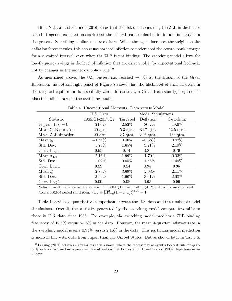
Table 4. Unconditional Moments: Data versus Model

U.S. Data Model SimulationsStatistic 1988.Q1-2017.Q2 Targeted Deflation Switching

% periods it = 0 24.6% 2.52% 80.2% 19.6%Mean ZLB duration 29 qtrs. 5.3 qtrs. 34.7 qtrs. 12.5 qtrs.Max. ZLB duration 29 qtrs. 37 qtrs. 346 qtrs. 133 qtrs.Mean yt −1.44% 0.40% −0.38% 0.42%Std. Dev. 1.75% 1.65% 3.21% 2.19%Corr. Lag 1 0.95 0.74 0.81 0.79

Mean π4, t 2.16% 1.99% −1.70% 0.93%Std. Dev. 1.09% 0.85% 1.58% 1.46%Corr. Lag 1 0.89 0.84 0.95 0.95

Mean i∗t 2.83% 3.69% −2.63% 2.11%Std. Dev. 3.42% 1.90% 3.01% 2.90%Corr. Lag 1 0.99 0.98 0.98 0.99

Notes: The ZLB episode in U.S. data is from 2008.Q4 through 2015.Q4. Model results are computed

from a 300,000 period simulation. π4, t ≡ [Π3j=0(1 + πt−j)]0.25 − 1.

Table 4 provides a quantitative comparison between the U.S. data and the results of model

simulations. Overall, the statistics generated by the switching model compare favorably to

those in U.S. data since 1988. For example, the switching model predicts a ZLB binding

frequency of 19.6% versus 24.6% in the data. However, the mean 4-quarter inflation rate in

the switching model is only 0.93% versus 2.16% in the data. This particular model prediction

is more in line with data from Japan than the United States. But as shown later in Table 6,

22Lansing (2009) achieves a similar result in a model where the representative agent’s forecast rule for quar-terly inflation is based on a perceived law of motion that follows a Stock and Watson (2007) type time seriesprocess.

20

the mean 4-quarter inflation rate in the switching model can be increased by allowing r∗t to

dip further into negative territory during the simulations.

Using data from all advanced economies since 1950, Dordal-i-Carrera et al. (2016) estimate

an average ZLB binding frequency of 7.5% and an average duration for ZLB episodes of 14

quarters. Excluding the high inflation period from 1968 to 1984 serves to raise the average

ZLB binding frequency and the average ZLB duration to 10% and 18 quarters, respectively.

For the period of consistent U.S. monetary policy since 1988, the single ZLB episode lasted

29 quarters.

Figure 9 plots the distribution of ZLB durations in each model version. Unlike the tar-

geted equilibrium, the switching model can produce infrequent and long-lived ZLB episodes

in response to small, normally distributed shocks. The average ZLB duration in the switching

model is 12.5 quarters, with a maximum observed duration in the simulation of 133 quarters

(Table 4). From Figure 9, we see that a 29 quarter ZLB episode is an extremely rare event

in the targeted equilibrium but can occur with about 5% frequency in the switching model.

To account for infrequent and long-lived ZLB episodes in the targeted equilibrium, Dordal-i-

Carreras, et al. (2016) develop a model with large, infrequent, and long-lived shocks.23

When ω = 0.459, the exponentially-weighted moving average of quarterly inflation πt com-

puted from equation (13) provides a very good approximation of the 4-quarter inflation rate.

Although not shown in Table 4, the mean, standard deviation, and first-order autocorrelation

of πt in the switching model are 0.94%, 1.48%, and 0.90, respectively. These values are close

to the corresponding statistics for π4, t of 0.93%, 1.46%, and 0.95.

The mean weight on the targeted forecast rules in the switching model is 0.69 with a

standard deviation of 0.29. Larger values for the window length Tw that is used to compute

the RMSFE measure from equation (16) serve to reduce the frequency of regime switches

and thereby raise the mean 4-quarter inflation rate. For example, when Tw is increased to 16

quarters, the mean value of µt is higher at 0.78 and the standard deviation is lower at 0.22.

With Tw = 16, the ZLB binding frequency in the switching model drops to 12.3% and the

average ZLB duration is lower at 9.2 quarters. The mean value of π4, t increases to 1.24% from

0.93%.

Figure 10 plots simulations from each of the three model versions: targeted, deflation,

and switching. All three versions employ the same sequence of stochastic shocks. When the

weight on the targeted forecast rules starts dropping around period 1725, the switching model

23 In a New Keynesian model with physical capital, Dennis (2016) shows that the introduction of capitaladjustment costs can help to generate infrequent and long-lived ZLB episodes in the targeted equilibrium.

21

generates a negative desired nominal policy rate, a binding ZLB, brief deflation followed by

below-target inflation, and a highly negative output gap, reminiscent of the U.S. Great Reces-

sion and its aftermath (Figure 4). The severity of the recession in the switching model is due

to the larger response coeffi cients on the state variables rt−Etr∗t and νt in the deflation equi-librium decision rule for yt. Specifically, the response coeffi cient on rt − Etr∗t in the deflationequilibrium is 1.25 versus 0.59 in the targeted equilibrium. The corresponding response coef-

ficients on νt are 5.40 versus 3.22 (Appendices B and C). The deflation equilibrium response

coeffi cients have more influence as the forecast weight µt declines, causing adverse realizations

of rt − Etr∗t or νt to be transmitted more forcefully to the output gap.Evans, Honkapohja, and Mitra (2016) argue that the deflation equilibrium does not provide

a convincing explanation of the sluggish output recovery following the Great Recession because

the steady state level of real activity in the deflation equilibrium is not much below the steady

state level of real activity in the targeted equilibrium. However, their analysis does not take

into account that the real rate gap rt − Etr∗t in U.S. data has remained significantly negativesince the recession ended, as can be seen in the top left panel of Figure 4. A negative real

rate gap puts stronger downward pressure on yt in the deflation equilibrium, thus helping

to explain the sluggish output recovery in U.S. data. Moreover, as we saw from the data

replication exercise, putting some weight on the deflation equilibrium forecast rules can help

to explain the pattern of U.S. data, even if the deflation equilibrium is never fully realized.

As noted earlier, the agent in the switching model considers the ZLB to be occasionally

binding across regimes, but not within a given regime. Most of the time, the switching model

fluctuates in a state that can be described as a mixture of the two regimes. Each period, the

agent adjusts the forecast weight µt in a way that is perceived to improve forecast accuracy.

In such an environment, the agent’s failure to take into account a relatively rare within-regime

event should not have much impact on overall forecasting performance. Table 5 summarizes

the properties of the agent’s forecast errors in each of the three model versions. The forecast

error is given by errxt+1 = xt+1 − Ft xt+1 for xt+1 ∈ {yt+1, πt+1} , where Ft xt+1 is the valuepredicted by the local linear forecast rule or, in the case of the switching model, the weighted-

average forecast rule, (14) or (15). The properties of the agent’s forecast errors in the switching

model are not much different from those in the targeted equilibrium. Notably, the forecast

errors are close to white noise.

22

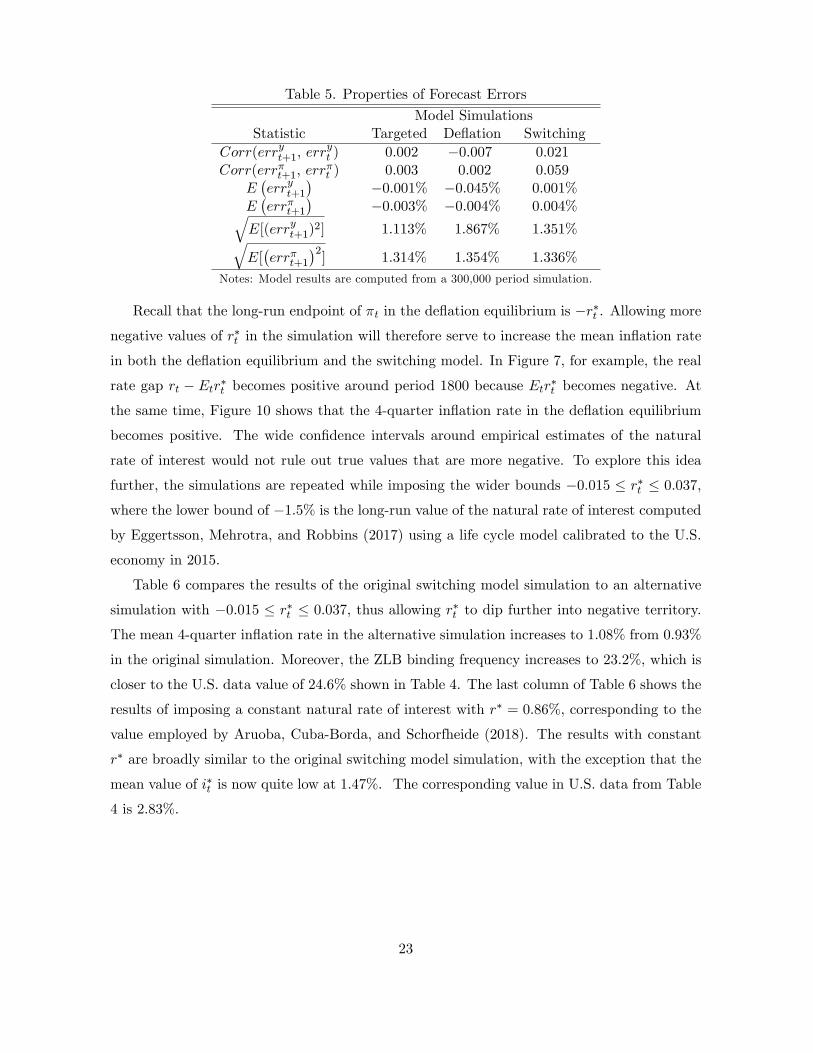
Table 5. Properties of Forecast Errors

Model SimulationsStatistic Targeted Deflation Switching

Corr(erryt+1, erryt ) 0.002 −0.007 0.021

Corr(errπt+1, errπt ) 0.003 0.002 0.059

E(erryt+1

)−0.001% −0.045% 0.001%

E(errπt+1

)−0.003% −0.004% 0.004%√

E[(erryt+1)2] 1.113% 1.867% 1.351%√

E[(errπt+1

)2] 1.314% 1.354% 1.336%

Notes: Model results are computed from a 300,000 period simulation.

Recall that the long-run endpoint of πt in the deflation equilibrium is −r∗t . Allowing morenegative values of r∗t in the simulation will therefore serve to increase the mean inflation rate

in both the deflation equilibrium and the switching model. In Figure 7, for example, the real

rate gap rt − Etr∗t becomes positive around period 1800 because Etr∗t becomes negative. Atthe same time, Figure 10 shows that the 4-quarter inflation rate in the deflation equilibrium

becomes positive. The wide confidence intervals around empirical estimates of the natural

rate of interest would not rule out true values that are more negative. To explore this idea

further, the simulations are repeated while imposing the wider bounds −0.015 ≤ r∗t ≤ 0.037,

where the lower bound of −1.5% is the long-run value of the natural rate of interest computed

by Eggertsson, Mehrotra, and Robbins (2017) using a life cycle model calibrated to the U.S.

economy in 2015.

Table 6 compares the results of the original switching model simulation to an alternative

simulation with −0.015 ≤ r∗t ≤ 0.037, thus allowing r∗t to dip further into negative territory.

The mean 4-quarter inflation rate in the alternative simulation increases to 1.08% from 0.93%

in the original simulation. Moreover, the ZLB binding frequency increases to 23.2%, which is

closer to the U.S. data value of 24.6% shown in Table 4. The last column of Table 6 shows the

results of imposing a constant natural rate of interest with r∗ = 0.86%, corresponding to the

value employed by Aruoba, Cuba-Borda, and Schorfheide (2018). The results with constant

r∗ are broadly similar to the original switching model simulation, with the exception that the

mean value of i∗t is now quite low at 1.47%. The corresponding value in U.S. data from Table

4 is 2.83%.

23

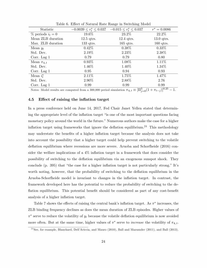
Table 6. Effect of Natural Rate Range in Switching Model

Statistic −0.0039 ≤ r∗t ≤ 0.037 −0.015 ≤ r∗t ≤ 0.037 r∗ = 0.0086

% periods it = 0 19.6% 23.2% 22.2%Mean ZLB duration 12.5 qtrs. 12.4 qtrs. 13.0 qtrs.Max. ZLB duration 133 qtrs. 165 qtrs. 160 qtrs.Mean yt 0.42% 0.38% 0.33%Std. Dev. 2.19% 2.23% 2.38%Corr. Lag 1 0.79 0.79 0.80

Mean π4, t 0.93% 1.08% 1.11%Std. Dev. 1.46% 1.40% 1.34%Corr. Lag 1 0.95 0.94 0.93

Mean i∗t 2.11% 1.75% 1.47%Std. Dev. 2.90% 2.88% 2.76Corr. Lag 1 0.99 0.99 0.99

Notes: Model results are computed from a 300,000 period simulation π4, t ≡ [Π3j=0(1 + πt−j)]0.25 − 1.

4.5 Effect of raising the inflation target

In a press conference held on June 14, 2017, Fed Chair Janet Yellen stated that determin-

ing the appropriate level of the inflation target “is one of the most important questions facing

monetary policy around the world in the future.”Numerous authors make the case for a higher

inflation target using frameworks that ignore the deflation equilibrium.24 This methodology

may understate the benefits of a higher inflation target because the analysis does not take

into account the possibility that a higher target could help prevent switching to the volatile

deflation equilibrium where recessions are more severe. Aruoba and Schorfheide (2016) con-

sider the welfare implications of a 4% inflation target in a framework that does consider the

possibility of switching to the deflation equilibrium via an exogenous sunspot shock. They

conclude (p. 395) that “the case for a higher inflation target is not particularly strong.” It’s

worth noting, however, that the probability of switching to the deflation equilibrium in the

Aruoba-Schorfheide model is invariant to changes in the inflation target. In contrast, the

framework developed here has the potential to reduce the probability of switching to the de-

flation equilibrium. This potential benefit should be considered as part of any cost-benefit

analysis of a higher inflation target.

Table 7 shows the effects of raising the central bank’s inflation target. As π∗ increases, the

ZLB binding frequency declines as does the mean duration of ZLB episodes. Higher values of

π∗ serve to reduce the volatility of yt because the volatile deflation equilibrium is now avoided

more often. But at the same time, higher values of π∗ serve to increase the volatility of π4, t.

24See, for example, Blanchard, Dell’Ariccia, and Mauro (2010), Ball and Mazumder (2011), and Ball (2013).

24

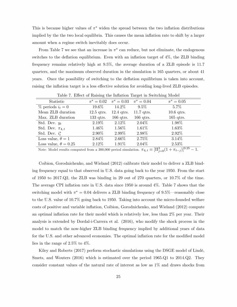
This is because higher values of π∗ widen the spread between the two inflation distributions

implied by the the two local equilibria. This causes the mean inflation rate to shift by a larger

amount when a regime switch inevitably does occur.

From Table 7 we see that an increase in π∗ can reduce, but not eliminate, the endogenous

switches to the deflation equilibrium. Even with an inflation target of 4%, the ZLB binding

frequency remains relatively high at 9.5%, the average duration of a ZLB episode is 11.7

quarters, and the maximum observed duration in the simulation is 165 quarters, or about 41

years. Once the possibility of switching to the deflation equilibrium is taken into account,

raising the inflation target is a less effective solution for avoiding long-lived ZLB episodes.

Table 7. Effect of Raising the Inflation Target in Switching Model

Statistic π∗ = 0.02 π∗ = 0.03 π∗ = 0.04 π∗ = 0.05

% periods it = 0 19.6% 14.2% 9.5% 5.7%Mean ZLB duration 12.5 qtrs. 12.4 qtrs. 11.7 qtrs. 10.6 qtrs.Max. ZLB duration 133 qtrs. 166 qtrs. 166 qtrs. 165 qtrs.Std. Dev. yt 2.19% 2.12% 2.04% 1.98%Std. Dev. π4, t 1.46% 1.56% 1.61% 1.63%Std. Dev. i∗t 2.90% 2.99% 2.98% 2.92%

Loss value, θ = 1 2.84% 2.66% 2.75% 3.14%Loss value, θ = 0.25 2.12% 1.91% 2.04% 2.53%

Note: Model results computed from a 300,000 period simulation. π4, t ≡ [Π3j=0(1 + πt−j)]0.25 − 1.

Coibion, Gorodnichenko, and Wieland (2012) calibrate their model to deliver a ZLB bind-

ing frequency equal to that observed in U.S. data going back to the year 1950. From the start

of 1950 to 2017.Q2, the ZLB was binding in 29 out of 270 quarters, or 10.7% of the time.

The average CPI inflation rate in U.S. data since 1950 is around 4%. Table 7 shows that the

switching model with π∗ = 0.04 delivers a ZLB binding frequency of 9.5%– reasonably close

to the U.S. value of 10.7% going back to 1950. Taking into account the micro-founded welfare

costs of positive and variable inflation, Coibion, Gorodnichenko, and Wieland (2012) compute

an optimal inflation rate for their model which is relatively low, less than 2% per year. Their

analysis is extended by Dordal-i-Carrera et al. (2016), who modify the shock process in the

model to match the now-higher ZLB binding frequency implied by additional years of data

for the U.S. and other advanced economies. The optimal inflation rate for the modified model

lies in the range of 2.5% to 4%.

Kiley and Roberts (2017) perform stochastic simulations using the DSGE model of Lindé,

Smets, and Wouters (2016) which is estimated over the period 1965.Q1 to 2014.Q2. They

consider constant values of the natural rate of interest as low as 1% and draws shocks from

25

the estimated distributions of the model. When monetary policy follows a simple Taylor (1999)

rule with no interest rate smoothing, they find that the ZLB binding frequency can be as high

as 32.6% with an mean ZLB duration of 12 quarters. The very high ZLB binding frequency

obtains even though the model solution considers only the targeted equilibrium. In contrast,

the simulations here deliver a baseline ZLB binding frequency in the switching model of 19.6%,

despite allowing for a natural rate of interest as low as −0.39% and further allowing for the

possibility of switches to the deflation equilibrium. The much higher ZLB binding frequency

obtained by Kiley and Roberts (2017) appears to be partly due to the shock distributions

which are based on the more-volatile U.S. data sample going back to 1965. Here, in contrast,

the shock distributions are based the more-recent sample period of consistent monetary policy

going back to 1988. Moreover, Kiley and Roberts (2017) do not allow for the possibility that

the natural rate of interest may drift above 1% in their simulations.

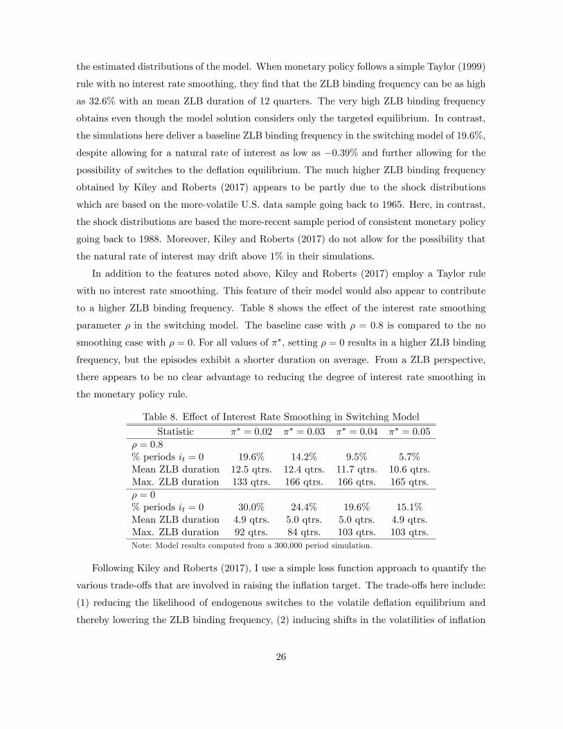
In addition to the features noted above, Kiley and Roberts (2017) employ a Taylor rule

with no interest rate smoothing. This feature of their model would also appear to contribute

to a higher ZLB binding frequency. Table 8 shows the effect of the interest rate smoothing

parameter ρ in the switching model. The baseline case with ρ = 0.8 is compared to the no

smoothing case with ρ = 0. For all values of π∗, setting ρ = 0 results in a higher ZLB binding

frequency, but the episodes exhibit a shorter duration on average. From a ZLB perspective,

there appears to be no clear advantage to reducing the degree of interest rate smoothing in

the monetary policy rule.

Table 8. Effect of Interest Rate Smoothing in Switching Model

Statistic π∗ = 0.02 π∗ = 0.03 π∗ = 0.04 π∗ = 0.05

ρ = 0.8% periods it = 0 19.6% 14.2% 9.5% 5.7%Mean ZLB duration 12.5 qtrs. 12.4 qtrs. 11.7 qtrs. 10.6 qtrs.Max. ZLB duration 133 qtrs. 166 qtrs. 166 qtrs. 165 qtrs.ρ = 0% periods it = 0 30.0% 24.4% 19.6% 15.1%Mean ZLB duration 4.9 qtrs. 5.0 qtrs. 5.0 qtrs. 4.9 qtrs.Max. ZLB duration 92 qtrs. 84 qtrs. 103 qtrs. 103 qtrs.Note: Model results computed from a 300,000 period simulation.

Following Kiley and Roberts (2017), I use a simple loss function approach to quantify the

various trade-offs that are involved in raising the inflation target. The trade-offs here include:

(1) reducing the likelihood of endogenous switches to the volatile deflation equilibrium and

thereby lowering the ZLB binding frequency, (2) inducing shifts in the volatilities of inflation

26

and the output gap, and (3) introducing economic distortions that come from a higher average

inflation. The loss function takes the form

Loss = E{

[π4, t − 0.02]2 + θ [yt − 0.02 (1− β) /κ]2}, (22)

where 0.02 and 0.02 (1− β) /κ are the long-run endpoints in the targeted equilibrium when

π∗ = 0.02, as shown in Table 1. The presumption is that the central bank in the baseline

calibration with π∗ = 0.02 has chosen to target the “optimal”levels of π4, t and yt. Hence, any

shift away from the original target values when adopting π∗ > 0.02 would introduce economic

distortions that are taken into account by the loss function. Also following Kiley and Roberts

(2017), I consider two values for the weight θ on the second term that captures the loss

from output gap deviations. The bottom rows of Table 7 show that the simple loss function

approach would favor a modest increase in the central bank’s inflation target. Specifically, the

loss function is minimized at π∗ = 0.03 when θ = 1 or θ = 0.25.

4.6 Adaptive learning in a simplified model

Up to this point, I have assumed that the representative agent has full knowledge of the

local linear forecast rules associated with each of the two equilibria. While the full-knowledge

assumption is standard in models with a unique equilibrium, the computational burden on the

agent is higher in the present context. To relax the full-knowledge assumption, I introduce an

adaptive learning algorithm in a simplified version of the model. Starting from the original

model, the simplified model imposes ρ = 0, ω = 1, ρν = ρu = 0, and ση = 0. These settings

eliminate i∗t−1 and πt−1 as state variables, eliminate the persistence in the shocks νt and ut,

and cause the natural rate of interest r∗ to be constant. I set r∗ = 0.0086, corresponding to the

constant value employed by Aruoba, Cuba-Borda, and Schorfheide (2018). Other parameter

values are identical to those in the original model. The theoretical decision rules for each of

the two local rational expectations equilibria are shown in Appendix D.

The learning agent employs decision rules that are estimated in real-time using model-

generated data. The resulting dynamics are self-referential because the agent’s current decision

rules influence the data generated by the model and thereby influence the estimated decision

rules in subsequent periods. An equilibrium is said to be “learnable”if the estimated decision

rules converge to the theoretical decision rules implied by the rational expectations solution.25

25Christiano, Eichenbaum, and Johanssen (2016) consider a more specialized learning experiment in whichthe ZLB is already binding due to a fundamental shock. Given this condition, they investigate whether variouslearning algorithms converge to either a high inflation or a low inflation equilibrium.

27

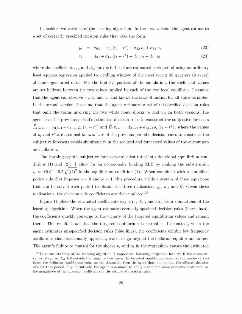
I consider two versions of the learning algorithm. In the first version, the agent estimates

a set of correctly specified decision rules that take the form:

yt = c 0,t + c 1,t (rt − r∗) + c 2,t νt + c 3,t ut, (23)

πt = d0,t + d1,t (rt − r∗) + d2,t νt + d3,t ut, (24)

where the coeffi cients ci,t and di,t for i = 0, 1, 2, 3 are estimated each period using an ordinary

least squares regression applied to a rolling window of the most recent 32 quarters (8 years)

of model-generated data. For the first 32 quarters of the simulation, the coeffi cient values

are set halfway between the two values implied by each of the two local equilibria. I assume

that the agent can observe rt, νt, and ut and knows the laws of motion for all state variables.

In the second version, I assume that the agent estimates a set of misspecified decision rules

that omit the terms involving the two white noise shocks νt and ut. In both versions, the

agent uses the previous period’s estimated decision rules to construct the subjective forecasts

Et yt+1 = c 0,t−1 + c 1,t−1ρr (rt − r∗) and Et πt+1 = d0,t−1 + d1,t−1ρr (rt − r∗) , where the valuesof ρr and r

∗ are assumed known. Use of the previous period’s decision rules to construct the

subjective forecasts avoids simultaneity in the realized and forecasted values of the output gap

and inflation.

The learning agent’s subjective forecasts are substituted into the global equilibrium con-

ditions (1) and (2). I allow for an occasionally binding ZLB by making the substitution

it = 0.5 i∗t + 0.5√

(i∗t )2 in the equilibrium condition (1). When combined with a simplified

policy rule that imposes ρ = 0 and ω = 1, this procedure yields a system of three equations

that can be solved each period to obtain the three realizations yt, πt, and i∗t . Given these

realizations, the decision rule coeffi cients are then updated.26

Figure 11 plots the estimated coeffi cients c 0,t, c 1,t, d0,t, and d1,t from simulations of the

learning algorithm. When the agent estimates correctly specified decision rules (black lines),

the coeffi cients quickly converge to the vicinity of the targeted equilibrium values and remain

there. This result shows that the targeted equilibrium is learnable. In contrast, when the

agent estimates misspecified decision rules (blue lines), the coeffi cients exhibit low frequency

oscillations that occasionally approach, reach, or go beyond the deflation equilibrium values.

The agent’s failure to control for the shocks νt and ut in the regressions causes the estimated

26To ensure stability of the learning algorithm, I impose the following projection facility: If the estimatedvalues of c0,t or d0,t fall outside the range of two times the targeted equilibrium value on the upside or twotimes the deflation equilibrium value on the downside, then the agent does not update the affected decisionrule for that period only. Intuitively, the agent is assumed to apply a common sense economic restriction onthe magnitude of the intercept coeffi cients in the estimated decision rules.

28

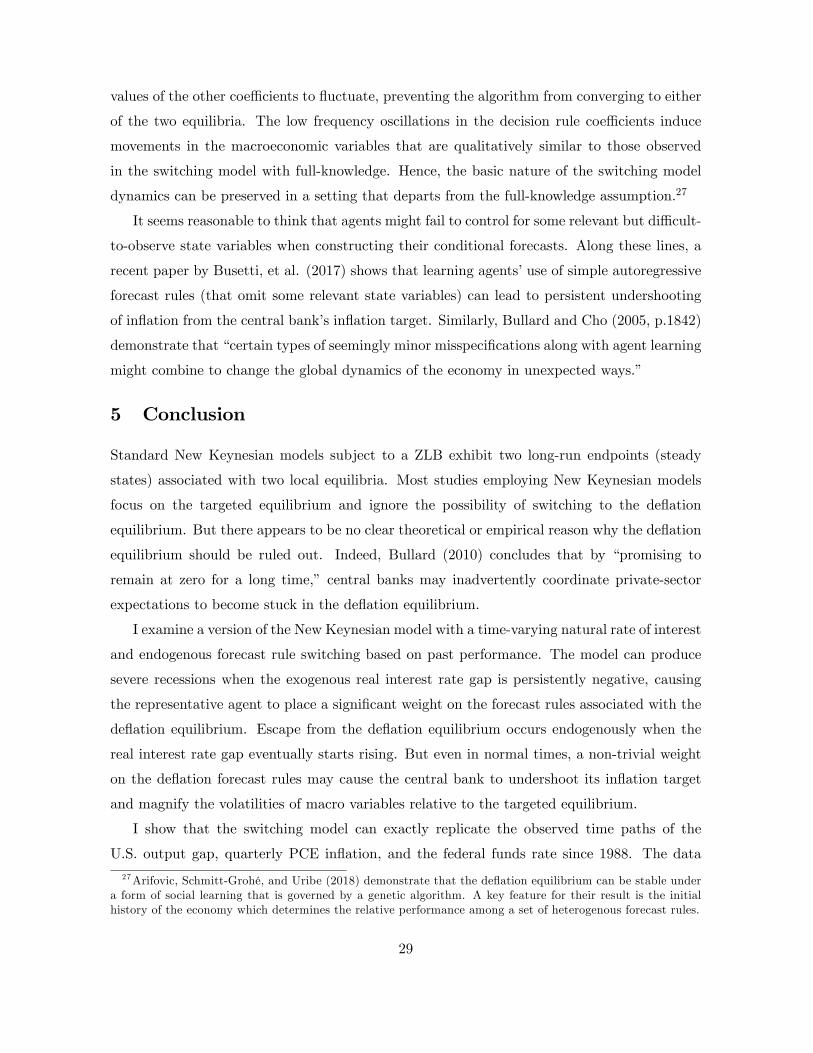
values of the other coeffi cients to fluctuate, preventing the algorithm from converging to either

of the two equilibria. The low frequency oscillations in the decision rule coeffi cients induce

movements in the macroeconomic variables that are qualitatively similar to those observed

in the switching model with full-knowledge. Hence, the basic nature of the switching model

dynamics can be preserved in a setting that departs from the full-knowledge assumption.27

It seems reasonable to think that agents might fail to control for some relevant but diffi cult-

to-observe state variables when constructing their conditional forecasts. Along these lines, a

recent paper by Busetti, et al. (2017) shows that learning agents’use of simple autoregressive

forecast rules (that omit some relevant state variables) can lead to persistent undershooting

of inflation from the central bank’s inflation target. Similarly, Bullard and Cho (2005, p.1842)

demonstrate that “certain types of seemingly minor misspecifications along with agent learning

might combine to change the global dynamics of the economy in unexpected ways.”

5 Conclusion

Standard New Keynesian models subject to a ZLB exhibit two long-run endpoints (steady

states) associated with two local equilibria. Most studies employing New Keynesian models

focus on the targeted equilibrium and ignore the possibility of switching to the deflation

equilibrium. But there appears to be no clear theoretical or empirical reason why the deflation

equilibrium should be ruled out. Indeed, Bullard (2010) concludes that by “promising to

remain at zero for a long time,” central banks may inadvertently coordinate private-sector

expectations to become stuck in the deflation equilibrium.

I examine a version of the New Keynesian model with a time-varying natural rate of interest

and endogenous forecast rule switching based on past performance. The model can produce

severe recessions when the exogenous real interest rate gap is persistently negative, causing

the representative agent to place a significant weight on the forecast rules associated with the

deflation equilibrium. Escape from the deflation equilibrium occurs endogenously when the

real interest rate gap eventually starts rising. But even in normal times, a non-trivial weight

on the deflation forecast rules may cause the central bank to undershoot its inflation target

and magnify the volatilities of macro variables relative to the targeted equilibrium.

I show that the switching model can exactly replicate the observed time paths of the

U.S. output gap, quarterly PCE inflation, and the federal funds rate since 1988. The data

27Arifovic, Schmitt-Grohé, and Uribe (2018) demonstrate that the deflation equilibrium can be stable undera form of social learning that is governed by a genetic algorithm. A key feature for their result is the initialhistory of the economy which determines the relative performance among a set of heterogenous forecast rules.

29

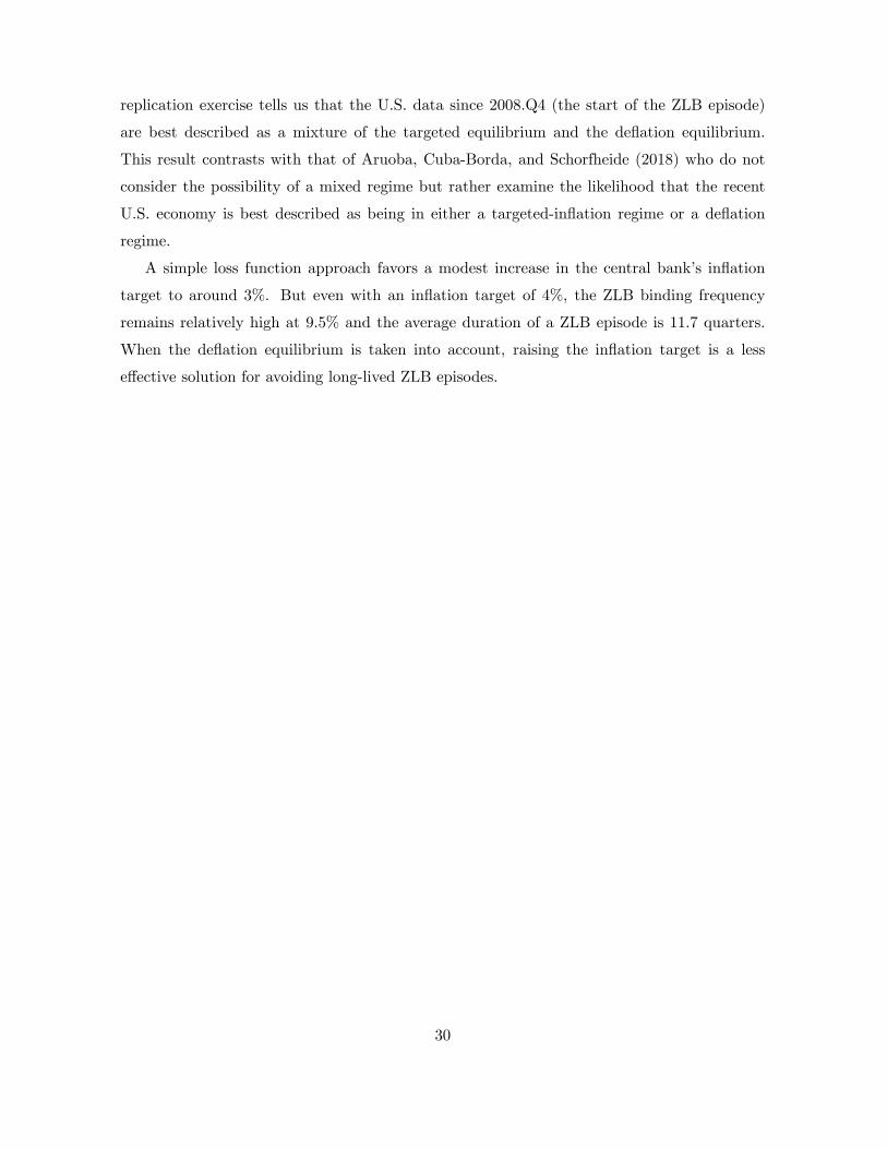
replication exercise tells us that the U.S. data since 2008.Q4 (the start of the ZLB episode)

are best described as a mixture of the targeted equilibrium and the deflation equilibrium.

This result contrasts with that of Aruoba, Cuba-Borda, and Schorfheide (2018) who do not

consider the possibility of a mixed regime but rather examine the likelihood that the recent

U.S. economy is best described as being in either a targeted-inflation regime or a deflation

regime.

A simple loss function approach favors a modest increase in the central bank’s inflation

target to around 3%. But even with an inflation target of 4%, the ZLB binding frequency

remains relatively high at 9.5% and the average duration of a ZLB episode is 11.7 quarters.

When the deflation equilibrium is taken into account, raising the inflation target is a less

effective solution for avoiding long-lived ZLB episodes.

30

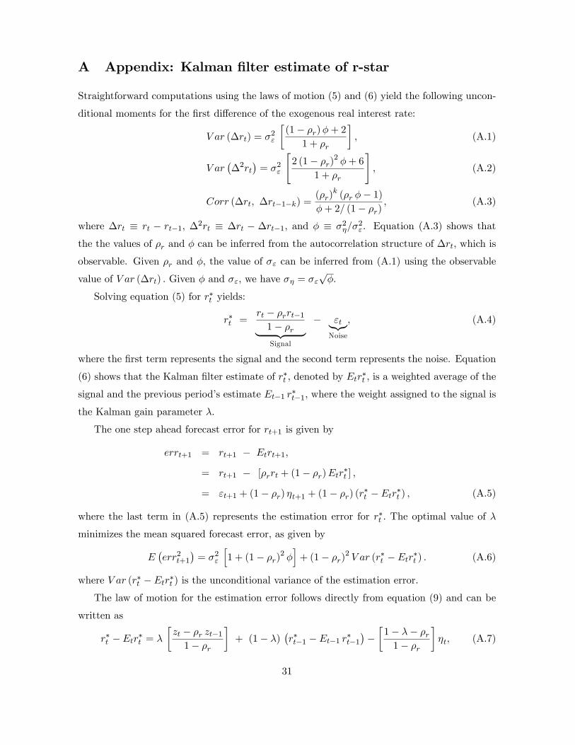
A Appendix: Kalman filter estimate of r-star

Straightforward computations using the laws of motion (5) and (6) yield the following uncon-

ditional moments for the first difference of the exogenous real interest rate:

V ar (∆rt) = σ2ε

[(1− ρr)φ+ 2

1 + ρr

], (A.1)

V ar(∆2rt

)= σ2ε

[2 (1− ρr)2 φ+ 6

1 + ρr

], (A.2)

Corr (∆rt, ∆rt−1−k) =(ρr)

k (ρr φ− 1)

φ+ 2/ (1− ρr), (A.3)

where ∆rt ≡ rt − rt−1, ∆2rt ≡ ∆rt − ∆rt−1, and φ ≡ σ2η/σ2ε. Equation (A.3) shows that

the the values of ρr and φ can be inferred from the autocorrelation structure of ∆rt, which is

observable. Given ρr and φ, the value of σε can be inferred from (A.1) using the observable

value of V ar (∆rt) . Given φ and σε, we have ση = σε√φ.

Solving equation (5) for r∗t yields:

r∗t =rt − ρrrt−1

1− ρr︸ ︷︷ ︸Signal

− εt︸︷︷︸Noise

, (A.4)

where the first term represents the signal and the second term represents the noise. Equation

(6) shows that the Kalman filter estimate of r∗t , denoted by Etr∗t , is a weighted average of the

signal and the previous period’s estimate Et−1 r∗t−1, where the weight assigned to the signal is

the Kalman gain parameter λ.

The one step ahead forecast error for rt+1 is given by

errt+1 = rt+1 − Etrt+1,

= rt+1 − [ρrrt + (1− ρr)Etr∗t ] ,

= εt+1 + (1− ρr) ηt+1 + (1− ρr) (r∗t − Etr∗t ) , (A.5)

where the last term in (A.5) represents the estimation error for r∗t . The optimal value of λ

minimizes the mean squared forecast error, as given by

E(err2t+1

)= σ2ε

[1 + (1− ρr)2 φ

]+ (1− ρr)2 V ar (r∗t − Etr∗t ) . (A.6)

where V ar (r∗t − Etr∗t ) is the unconditional variance of the estimation error.The law of motion for the estimation error follows directly from equation (9) and can be

written as

r∗t − Etr∗t = λ

[zt − ρr zt−1

1− ρr

]+ (1− λ)

(r∗t−1 − Et−1 r∗t−1

)−[

1− λ− ρr1− ρr

]ηt, (A.7)

31

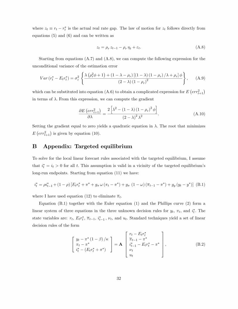
where zt ≡ rt − r∗t is the actual real rate gap. The law of motion for zt follows directly fromequations (5) and (6) and can be written as

zt = ρr zt−1 − ρr ηt + εt. (A.8)

Starting from equations (A.7) and (A.8), we can compute the following expression for the

unconditional variance of the estimation error

V ar (r∗t − Etr∗t ) = σ2ε

{λ(ρ2rφ+ 1

)+ (1− λ− ρr) [(1− λ) (1− ρr) /λ+ ρr]φ

(2− λ) (1− ρr)2

}, (A.9)

which can be substituted into equation (A.6) to obtain a complicated expression for E(err2t+1

)in terms of λ. From this expression, we can compute the gradient

∂E(err2t+1

)∂λ

=2[λ2 − (1− λ) (1− ρr)2 φ

](2− λ)2 λ2

. (A.10)

Setting the gradient equal to zero yields a quadratic equation in λ. The root that minimizes

E(err2t+1

)is given by equation (10).

B Appendix: Targeted equilibrium

To solve for the local linear forecast rules associated with the targeted equilibrium, I assume

that i∗t = it > 0 for all t. This assumption is valid in a vicinity of the targeted equilibrium’s

long-run endpoints. Starting from equation (11) we have:

i∗t = ρi∗t−1+ (1− ρ) [Etr∗t + π∗ + gπ ω (πt − π∗) + gπ (1− ω) (πt−1 − π∗) + gy (yt − y∗)] (B.1)

where I have used equation (12) to eliminate πt.

Equation (B.1) together with the Euler equation (1) and the Phillips curve (2) form a

linear system of three equations in the three unknown decision rules for yt, πt, and i∗t . The

state variables are: rt, Etr∗t , πt−1, i∗t−1 , νt, and ut. Standard techniques yield a set of linear

decision rules of the form

yt − π∗ (1− β) /κπt − π∗i∗t − (Etr

∗t + π∗)

= A

rt − Etr∗tπt−1 − π∗i∗t−1 − Etr∗t − π∗νtut

, (B.2)

32

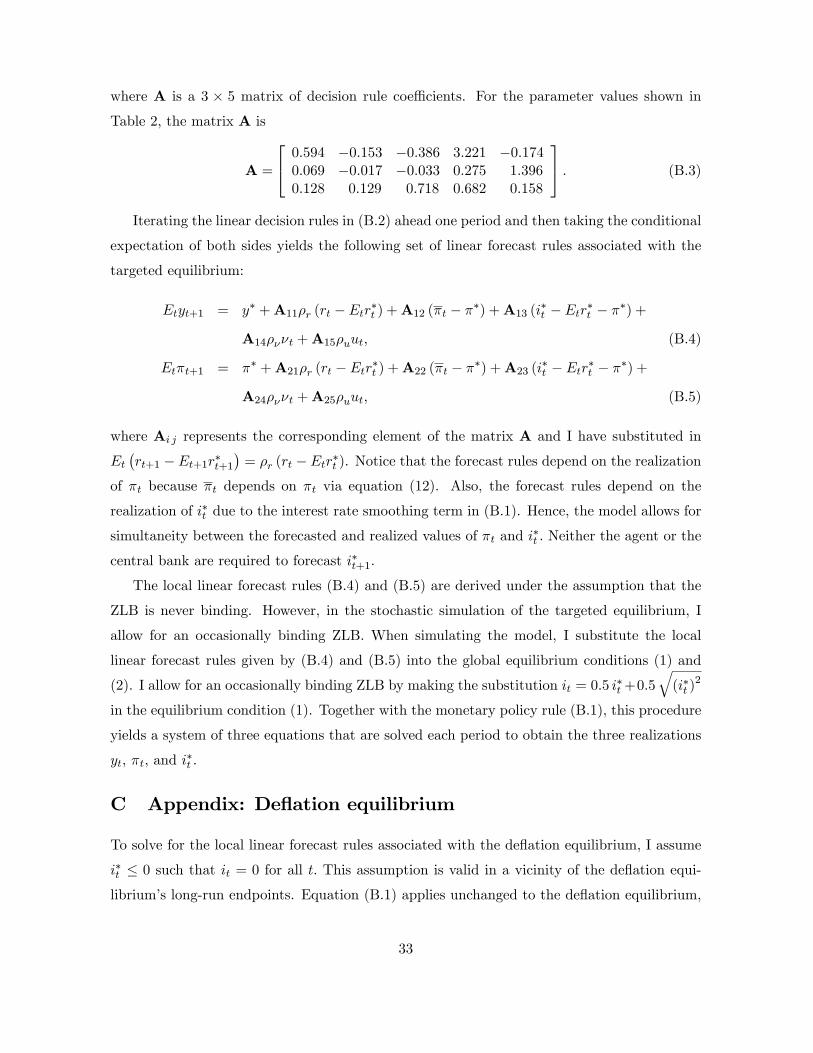
where A is a 3 × 5 matrix of decision rule coeffi cients. For the parameter values shown in

Table 2, the matrix A is

A =

0.594 −0.153 −0.386 3.221 −0.1740.069 −0.017 −0.033 0.275 1.3960.128 0.129 0.718 0.682 0.158

. (B.3)

Iterating the linear decision rules in (B.2) ahead one period and then taking the conditional

expectation of both sides yields the following set of linear forecast rules associated with the

targeted equilibrium:

Etyt+1 = y∗ +A11ρr (rt − Etr∗t ) +A12 (πt − π∗) +A13 (i∗t − Etr∗t − π∗) +

A14ρννt +A15ρuut, (B.4)

Etπt+1 = π∗ +A21ρr (rt − Etr∗t ) +A22 (πt − π∗) +A23 (i∗t − Etr∗t − π∗) +

A24ρννt +A25ρuut, (B.5)

where Ai j represents the corresponding element of the matrix A and I have substituted in

Et(rt+1 − Et+1r∗t+1

)= ρr (rt − Etr∗t ). Notice that the forecast rules depend on the realization

of πt because πt depends on πt via equation (12). Also, the forecast rules depend on the

realization of i∗t due to the interest rate smoothing term in (B.1). Hence, the model allows for

simultaneity between the forecasted and realized values of πt and i∗t . Neither the agent or the

central bank are required to forecast i∗t+1.

The local linear forecast rules (B.4) and (B.5) are derived under the assumption that the

ZLB is never binding. However, in the stochastic simulation of the targeted equilibrium, I

allow for an occasionally binding ZLB. When simulating the model, I substitute the local

linear forecast rules given by (B.4) and (B.5) into the global equilibrium conditions (1) and

(2). I allow for an occasionally binding ZLB by making the substitution it = 0.5 i∗t +0.5√

(i∗t )2

in the equilibrium condition (1). Together with the monetary policy rule (B.1), this procedure

yields a system of three equations that are solved each period to obtain the three realizations

yt, πt, and i∗t .

C Appendix: Deflation equilibrium

To solve for the local linear forecast rules associated with the deflation equilibrium, I assume

i∗t ≤ 0 such that it = 0 for all t. This assumption is valid in a vicinity of the deflation equi-

librium’s long-run endpoints. Equation (B.1) applies unchanged to the deflation equilibrium,

33

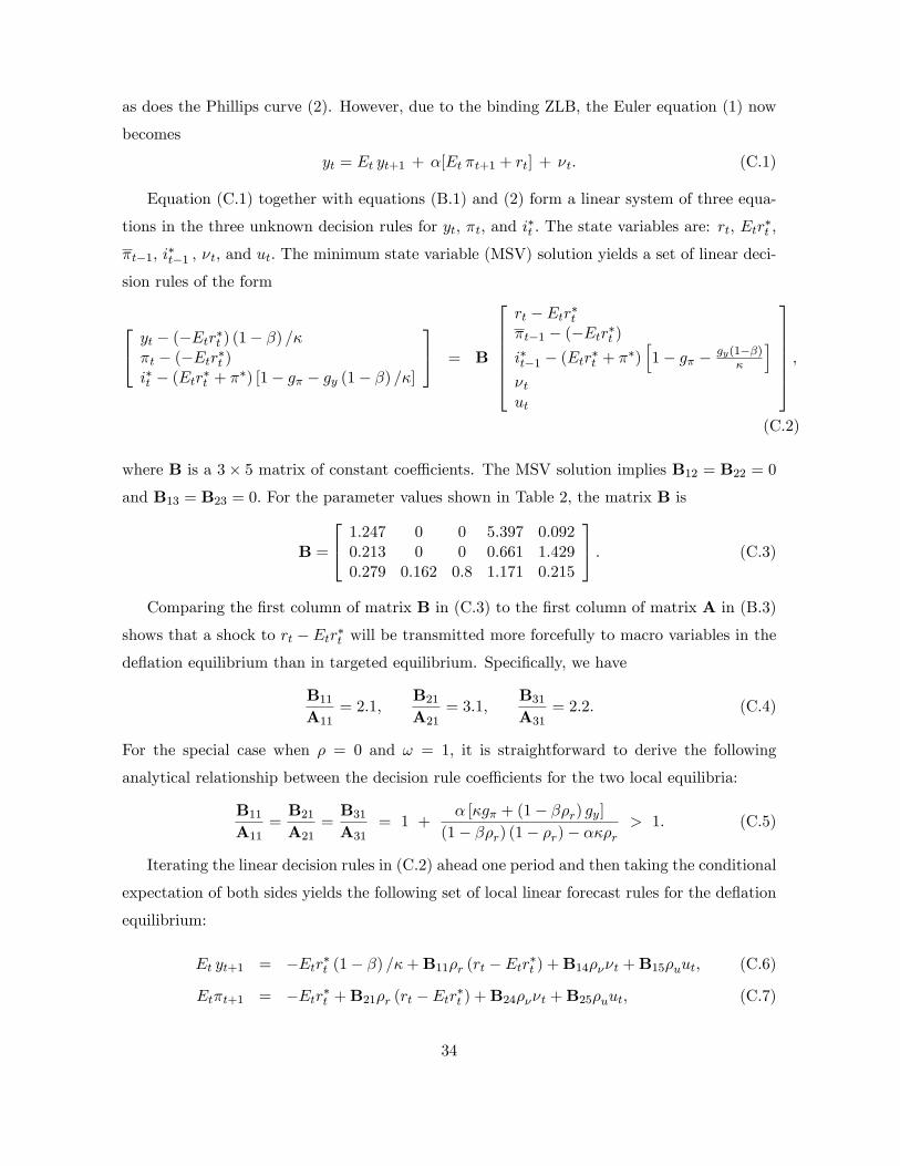
as does the Phillips curve (2). However, due to the binding ZLB, the Euler equation (1) now

becomes

yt = Et yt+1 + α[Et πt+1 + rt] + νt. (C.1)

Equation (C.1) together with equations (B.1) and (2) form a linear system of three equa-

tions in the three unknown decision rules for yt, πt, and i∗t . The state variables are: rt, Etr∗t ,

πt−1, i∗t−1 , νt, and ut. The minimum state variable (MSV) solution yields a set of linear deci-

sion rules of the form

yt − (−Etr∗t ) (1− β) /κπt − (−Etr∗t )i∗t − (Etr

∗t + π∗) [1− gπ − gy (1− β) /κ]

= B

rt − Etr∗tπt−1 − (−Etr∗t )i∗t−1 − (Etr

∗t + π∗)

[1− gπ − gy(1−β)

κ

]νtut

,(C.2)

where B is a 3× 5 matrix of constant coeffi cients. The MSV solution implies B12 = B22 = 0

and B13 = B23 = 0. For the parameter values shown in Table 2, the matrix B is

B =

1.247 0 0 5.397 0.0920.213 0 0 0.661 1.4290.279 0.162 0.8 1.171 0.215

. (C.3)

Comparing the first column of matrix B in (C.3) to the first column of matrix A in (B.3)

shows that a shock to rt − Etr∗t will be transmitted more forcefully to macro variables in thedeflation equilibrium than in targeted equilibrium. Specifically, we have

B11A11

= 2.1,B21A21

= 3.1,B31A31

= 2.2. (C.4)

For the special case when ρ = 0 and ω = 1, it is straightforward to derive the following

analytical relationship between the decision rule coeffi cients for the two local equilibria:

B11A11

=B21A21

=B31A31

= 1 +α [κgπ + (1− βρr) gy]

(1− βρr) (1− ρr)− ακρr> 1. (C.5)

Iterating the linear decision rules in (C.2) ahead one period and then taking the conditional

expectation of both sides yields the following set of local linear forecast rules for the deflation

equilibrium:

Et yt+1 = −Etr∗t (1− β) /κ+B11ρr (rt − Etr∗t ) +B14ρννt +B15ρuut, (C.6)

Etπt+1 = −Etr∗t +B21ρr (rt − Etr∗t ) +B24ρννt +B25ρuut, (C.7)

34

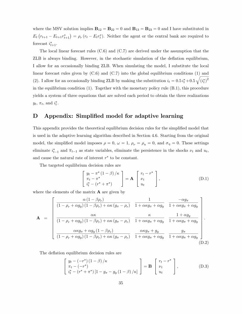
where the MSV solution implies B12 = B22 = 0 and B13 = B23 = 0 and I have substituted in

Et(rt+1 − Et+1r∗t+1

)= ρr (rt − Etr∗t ). Neither the agent or the central bank are required to

forecast i∗t+1.

The local linear forecast rules (C.6) and (C.7) are derived under the assumption that the

ZLB is always binding. However, in the stochastic simulation of the deflation equilibrium,

I allow for an occasionally binding ZLB. When simulating the model, I substitute the local

linear forecast rules given by (C.6) and (C.7) into the global equilibrium conditions (1) and

(2). I allow for an occasionally binding ZLB by making the substitution it = 0.5 i∗t +0.5√

(i∗t )2

in the equilibrium condition (1). Together with the monetary policy rule (B.1), this procedure

yields a system of three equations that are solved each period to obtain the three realizations

yt, πt, and i∗t .

D Appendix: Simplified model for adaptive learning

This appendix provides the theoretical equilibrium decision rules for the simplified model that

is used in the adaptive learning algorithm described in Section 4.6. Starting from the original

model, the simplified model imposes ρ = 0, ω = 1, ρν = ρu = 0, and ση = 0. These settings

eliminate i∗t−1 and πt−1 as state variables, eliminate the persistence in the shocks νt and ut,

and cause the natural rate of interest r∗ to be constant.

The targeted equilibrium decision rules are yt − π∗ (1− β) /κπt − π∗i∗t − (r∗ + π∗)

= A

rt − r∗νtut

, (D.1)

where the elements of the matrix A are given by

A =

α (1− βρr)(1− ρr + αgy) (1− βρr) + ακ (gπ − ρr)

1

1 + ακgπ + αgy

−αgπ1 + ακgπ + αgy

ακ

(1− ρr + αgy) (1− βρr) + ακ (gπ − ρr)κ

1 + ακgπ + αgy

1 + αgy1 + ακgπ + αgy

ακgπ + αgy (1− βρr)(1− ρr + αgy) (1− βρr) + ακ (gπ − ρr)

ακgπ + gy1 + ακgπ + αgy

gπ1 + ακgπ + αgy

.

(D.2)

The deflation equilibrium decision rules are yt − (−r∗) (1− β) /κπt − (−r∗)i∗t − (r∗ + π∗) [1− gπ − gy (1− β) /κ]

= B

rt − r∗νtut

, (D.3)

35

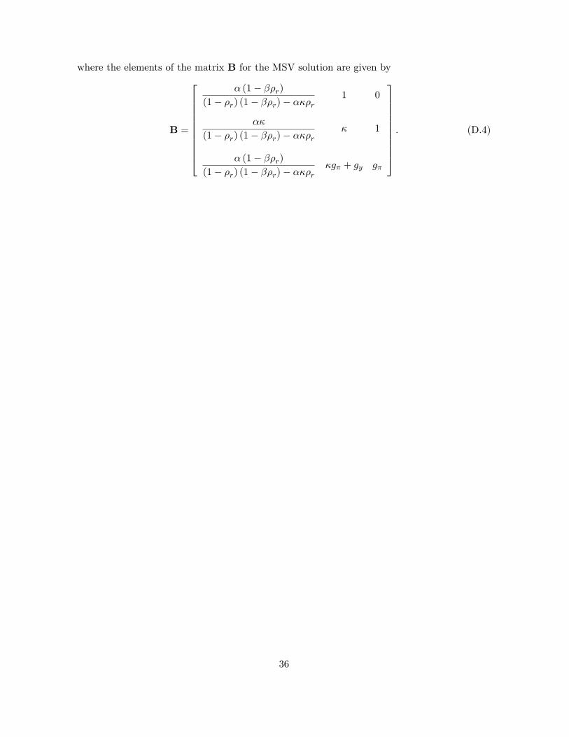
where the elements of the matrix B for the MSV solution are given by

B =

α (1− βρr)(1− ρr) (1− βρr)− ακρr

1 0

ακ

(1− ρr) (1− βρr)− ακρrκ 1

α (1− βρr)(1− ρr) (1− βρr)− ακρr

κgπ + gy gπ

. (D.4)

36

ReferencesAdam, K. and R. Billi 2007 Discretionary Monetary Policy and the Zero Lower Bound onNominal Interest Rates, Journal of Monetary Economics 54, 728-752.

Alstadheim, R. and D.W. Henderson 2006 Price-Level Determinacy, Lower Bounds on theNominal Interest Rate, and Liquidity Traps, B.E. Journal of Macroeconomics, Contributionsto Macroeconomics 6(1), Article 12.

Altig, D., N. Parker, and B. Meyer 2017 The Fed’s Inflation Goal: What Does the PublicKnow? Federal Reserve Bank of Atlanta, Macroblog (April 19).

Arifovic, J., S. Schmitt-Grohé, and M. Uribe 2018 Learning to Live in a Liquidity Trap,Journal of Economic Dynamics and Control, forthcoming.

Aruoba, S.B., P. Cuba-Borda, and F. Schorfheide 2018 Macroeconomic Dynamics Near theZLB: A Tale of Two Countries, Review of Economic Studies, 85, 87-118.

Aruoba, S.B. and F. Schorfheide 2016 Inflation During and After the Zero Lower Bound, inFederal Reserve Bank of Kansas City 2015 Economic Policy Symposium Proceedings, InflationDynamics and Monetary Policy, pp. 359-436.

Ball, L., and S. Mazumder 2011 Inflation Dynamics and the Great Recession, Brookings Paperson Economic Activity, Spring, , 337-402.

Ball L. 2013 The Case for Four Percent Inflation, Central Bank Review 13, 17-31.

Barsky, R., A. Justiniano, and L. Melosi 2014 The Natural Rate of Interest and Its Usefulnessfor Monetary Policy, American Economic Review: Papers & Proceedings 104(5), 37-43.

Basu, S. and B. Bundick 2015 Endogenous Volatility at the Zero Lower Bound: Implicationsfor Stabilization Policy, NBER Working Paper 21838.

Benhabib, J., S. Schmitt-Grohé, and M. Uribe 2001a Monetary Policy and Multiple Equilibria,American Economic Review 91, 167-186.

Benhabib, J., S. Schmitt-Grohé, and M. Uribe 2001b The Perils of Taylor Rules, Journal ofEconomic Theory 96, 40-69.

Benhabib, J. G.W. Evans and S. Honkapohja 2014 Liquidity Traps and Expectation Dynamics:Fiscal Stimulus or Fiscal Austerity? Journal of Economic Dynamics and Control 45, 220-238.

Binning, A. and J. Maih 2017 Modelling Occasionally Binding Constraints Using Regime-Switching, Norges Bank Working Paper 2017-23.

Busetti, F., D. Delle Monache, A. Gerali, and A. Locarno 2017 Trust but Verify: De-anchoringof Inflation Expectations under Learning and Heterogeneity, European Central Bank WorkingPaper 1994.

Blanchard, O., G. Dell’Ariccia, and P. Mauro 2010 Rethinking Macroeconomic Policy, Journalof Money, Credit and Banking 42(s1), 199-215.

Bullard, J. 2010 Seven Faces of “The Peril,” Federal Reserve Bank of St. Louis, Review,September/October, 92, 339-352.

Bullard, J. and I.-K. Cho,I.-K. 2005 Escapist Policy Rules, Journal of Economic Dynamicsand Control 29, 1841-1866.

Campbell, J.Y. and N.G. Mankiw 1989 Consumption, Income, and Interest Rates: Reinterpret-ing the Time Series Evidence, in O.J. Blanchard and S. Fischer (eds.), NBER MacroeconomicsAnnual 1989, Volume 4. Cambridge MA: MIT Press, pp. 185-246.

37

Carlstrom, C.T. and T.S. Fuerst 2016 The Natural Rate of Interest in Taylor Rules, FederalReserve Bank of Cleveland Economic Commentary 2016-01 (March 22)

Christiano, L.J., M. Eichenbaum, and B.K. Johannsen 2016 Does the New Keynesian ModelHave a Uniqueness Problem?”Working Paper.

Chung, H., J.-P. Laforte, D. Reifschneider, and J.C. Williams 2012 Have We Underestimatedthe Likelihood and Severity of Zero Lower Bound Events? Journal of Money, Credit andBanking 44, 47-82.

Cochrane, J.H. 2017 Michelson-Morley, Fisher, and Occam: The Radical Implications of StableInflation at the Zero Bound, Hoover Institution, Working Paper.

Coibion, O., Y. Gorodnichenko, and J. Wieland 2012 The Optimal Inflation Rate in NewKeynesian models: Should Central Banks Raise Their Inflation Targets in Light of the ZeroLower Bound? Review of Economic Studies 79, 1371-1406.

Cúrdia, V., A. Ferrero, G.C. Ng, and A. Tambalotti 2015 Has U.S. Monetary Policy Trackedthe Effi cient Interest Rate? Journal of Monetary Economics 70, 72-83.

Dennis, R. 2016 Durations at the Zero Lower Bound, University of Glasgow, Working Paper.

Del Negro, M., D. Giannone, M.P. Giannoni, and A. Tambalotti 2017 Safety, Liquidity, andthe Natural Rate of Interest, Brookings Papers on Economic Activity (Spring), 235-294.

Dordal-i-Carreras, M., O. Coibion, Y. Gorodnichenko, J. Wieland 2016 Infrequent but Long-Lived Zero-Bound Episodes and the Optimal Rate of Inflation, Annual Review of Economics8, 497-520.

Dudley, W.C. 2015 The U.S. Economic Outlook and Monetary Policy, Remarks at the Eco-nomic Club of New York, New York City (November 12).

Eggertsson, G.B. and M. Woodford 2003 The Zero Bound on Interest Rates and OptimalMonetary Policy, Brookings Papers on Economic Activity 2003(1), 139-211.

Eggertsson, G.B. and S.R. Sing 2016 Log-linear Approximation versus an Exact Solution atthe ZLB in the New Keynesian Model, NBER Working Paper 22784.

Eggertsson, G.B., N.R. Mehrotra, and J.A. Robbins 2017 A Model of Secular Stagnation:Theory and Quantitative Evaluation, NBER Working Paper 23093.

Eusepi, S. 2007 Learnability and Monetary Policy: A Global Perspective, Journal of MonetaryEconomics 54, 1115-1131.

Evans, G.W. and S. Honkapohja 2005 Policy Interaction, Expectations and the LiquidityTrap, Review of Economic Dynamics 8, 303—323.

Evans, G.W., E. Guse, and, S. Honkapohja 2008 Liquidity Traps, Learning, and Stagnation,European Economic Review 52, 1438-1463.

Evans, G.W., S. Honkapohja, and K. Mitra 2016 Expectations, Stagnation and Fiscal Policy,Working Paper.

Evans, C., J. Fisher, F. Gourio, and S. Krane 2015 Risk Management for Monetary PolicyNear the Zero Lower Bound, Brookings Papers on Economic Activity (Spring), 141-196

Fischer, S. 2016 Monetary Policy, Financial Stability, and the Zero Lower Bound, Remarks atthe Annual Meeting of the American Economic Association, San Francisco, California (January3).

Garín, J., R. Lester, and E. Sims 2018 Raise Rates to Raise Inflation? Neo-Fisherianism inthe New Keynesian Model, Journal of Money Credit and Banking 50, 243-259.

38

Gelain, P., K.J. Lansing, and G.J. Natvik 2018 Explaining the Boom-Bust-Cycle in the U.S.Housing Market: A Reverse-Engineering Approach, Journal of Money Credit and Banking,forthcoming.

Guerrieri, L. and M. Iacoviello 2015 OccBin: A Toolkit for Solving Dynamic Models withOccasionally Binding Constraints Easily, Journal of Monetary Economics 70, 22—38.

Gust, C.J., B.K. Johannsen, and D. López-Salido 2017 Monetary Policy, Incomplete Informa-tion, and the Zero Lower Bound, IMF Economic Review 65, 37-70.

Hamilton, J.D., E.S. Harris, J. Hatzius, and K.D. West 2016 The Equilibrium Real FundsRate: Past, Present and Future, IMF Economic Review 64, 660-707.

Haubrich, J.G., G. Pennacchi, and P. Ritchken 2012 Inflation Expectations, Real Rates, andRisk Premia: Evidence from Inflation Swaps, Review of Financial Studies 25, 1588-1629.

Hills, T.S., T. Nakata, and S. Schmidt 2016 The Risky Steady State and the Interest RateLower Bound, Federal Reserve Board, Finance and Economics Discussion Series Paper 2016-009.

International Monetary Fund 2014 Perspectives on Global Real Interest Rates, Chapter 3 ofWorld Economic Outlook (WEO), Recovery Strengthens, Remains Uneven (April).

Jackson, L.E., K.L. Kliesen, and M.T. Owyang 2015 A Measure of Price Pressures, FederalReserve Bank of St. Louis Review 97(1), 25-52.

Kiley, M.T. 2015 What Can the Data Tell Us About the Equilibrium Real Interest Rate?Federal Reserve Board, Finance and Economics Discussion Series Paper 2015-077.

Kiley, M.T. and J.M. Roberts 2017 Monetary policy in a Low Interest Rate World, BrookingsPapers on Economic Activity (Spring), 317-372.

Kozicki, S. and P.A. Tinsley 2012 Effective Use of Survey Information in Estimating theEvolution of Expected Inflation Journal of Money Credit and Banking 44, 145-169.

Lansing, K.J. 2009 Time-Varying U.S. Inflation Dynamics and the New Keynesian PhillipsCurve, Review of Economic Dynamics 12, 304-326.

Lansing, K.J. 2016 Projecting the Long-Run Natural Rate of Interest, Federal Reserve Bankof San Francisco Economic Letter 2016-25 (August 29).

Lansing, K.J. 2017 R-star, Uncertainty, and Monetary Policy, Federal Reserve Bank of SanFrancisco Economic Letter 2017-16 (May 30).

Lansing, K.J. and S.F. LeRoy 2014 Risk Aversion, Investor Information, and Stock MarketVolatility, European Economic Review 70, 88-107.

Laubach, T. and J.C. Williams 2016 Measuring the Natural Rate of Interest Redux, BusinessEconomics 51, 257-267.

Lindé, J., F. Smets, and R. Wouters 2016 Challenges for Central Bank Macro Models, in J.B.Taylor and H. Uhlig (eds.), Handbook of Macroeconomics Volume 2. Amsterdam: Elsevier,pp. 2185-2262.

Lubik, T.A. and C. Matthes 2015 Calculating the Natural Rate of Interest: A Comparison ofTwo Alternative Approaches, Federal Reserve Bank of Richmond, Economic Brief (October15).

McCallum, B. 1999 Role of the Minimal State Variable Criterion in Rational ExpectationsModels, International Tax and Public Finance 6, 621—639.

McKay, A., E. Nakamura, and J. Steinsson 2016 The Discounted Euler Equation: A Note,

39

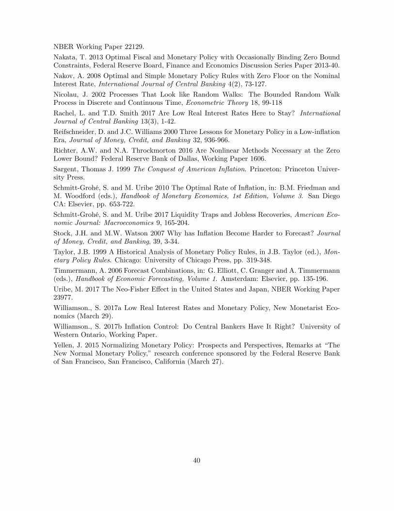
NBER Working Paper 22129.

Nakata, T. 2013 Optimal Fiscal and Monetary Policy with Occasionally Binding Zero BoundConstraints, Federal Reserve Board, Finance and Economics Discussion Series Paper 2013-40.

Nakov, A. 2008 Optimal and Simple Monetary Policy Rules with Zero Floor on the NominalInterest Rate, International Journal of Central Banking 4(2), 73-127.

Nicolau, J. 2002 Processes That Look like Random Walks: The Bounded Random WalkProcess in Discrete and Continuous Time, Econometric Theory 18, 99-118

Rachel, L. and T.D. Smith 2017 Are Low Real Interest Rates Here to Stay? InternationalJournal of Central Banking 13(3), 1-42.

Reifschneider, D. and J.C. Williams 2000 Three Lessons for Monetary Policy in a Low-inflationEra, Journal of Money, Credit, and Banking 32, 936-966.

Richter, A.W. and N.A. Throckmorton 2016 Are Nonlinear Methods Necessary at the ZeroLower Bound? Federal Reserve Bank of Dallas, Working Paper 1606.

Sargent, Thomas J. 1999 The Conquest of American Inflation. Princeton: Princeton Univer-sity Press.

Schmitt-Grohé, S. and M. Uribe 2010 The Optimal Rate of Inflation, in: B.M. Friedman andM. Woodford (eds.), Handbook of Monetary Economics, 1st Edition, Volume 3. San DiegoCA: Elsevier, pp. 653-722.

Schmitt-Grohé, S. and M. Uribe 2017 Liquidity Traps and Jobless Recoveries, American Eco-nomic Journal: Macroeconomics 9, 165-204.

Stock, J.H. and M.W. Watson 2007 Why has Inflation Become Harder to Forecast? Journalof Money, Credit, and Banking, 39, 3-34.

Taylor, J.B. 1999 A Historical Analysis of Monetary Policy Rules, in J.B. Taylor (ed.), Mon-etary Policy Rules. Chicago: University of Chicago Press, pp. 319-348.

Timmermann, A. 2006 Forecast Combinations, in: G. Elliott, C. Granger and A. Timmermann(eds.), Handbook of Economic Forecasting, Volume 1. Amsterdam: Elsevier, pp. 135-196.

Uribe, M. 2017 The Neo-Fisher Effect in the United States and Japan, NBER Working Paper23977.

Williamson., S. 2017a Low Real Interest Rates and Monetary Policy, New Monetarist Eco-nomics (March 29).

Williamson., S. 2017b Inflation Control: Do Central Bankers Have It Right? University ofWestern Ontario, Working Paper.

Yellen, J. 2015 Normalizing Monetary Policy: Prospects and Perspectives, Remarks at “TheNew Normal Monetary Policy,” research conference sponsored by the Federal Reserve Bankof San Francisco, San Francisco, California (March 27).

40

Figure 1: Nominal Interest Rates and Inflation in Four Countries

Nominal interest rates in the United States encountered the zero lower bound during the 1930s and from 2008.Q4though 2015.Q4. Nominal interest rates in Japan have remained near zero since 1998.Q3, except for the relativelybrief period from 2006.Q4 to 2008.Q3. Nominal interest rates in Switzerland have been zero or slightly negativesince 2008.Q4. Nominal interest rates in the United Kingdom have been approximately zero since 2009.Q1.Outside of these episodes, all four countries exhibit a strong positive correlation between nominal interest ratesand inflation, consistent with the Fisher relationship.

41

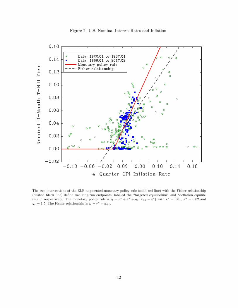
Figure 2: U.S. Nominal Interest Rates and Inflation

The two intersections of the ZLB-augmented monetary policy rule (solid red line) with the Fisher relationship(dashed black line) define two long-run endpoints, labeled the “targeted equilibrium” and “deflation equilib-rium,” respectively. The monetary policy rule is it = r∗ + π∗ + gπ (π4,t − π∗) with r∗ = 0.01, π∗ = 0.02 andgπ = 1.5. The Fisher relationship is it = r∗ + π4,t.

42

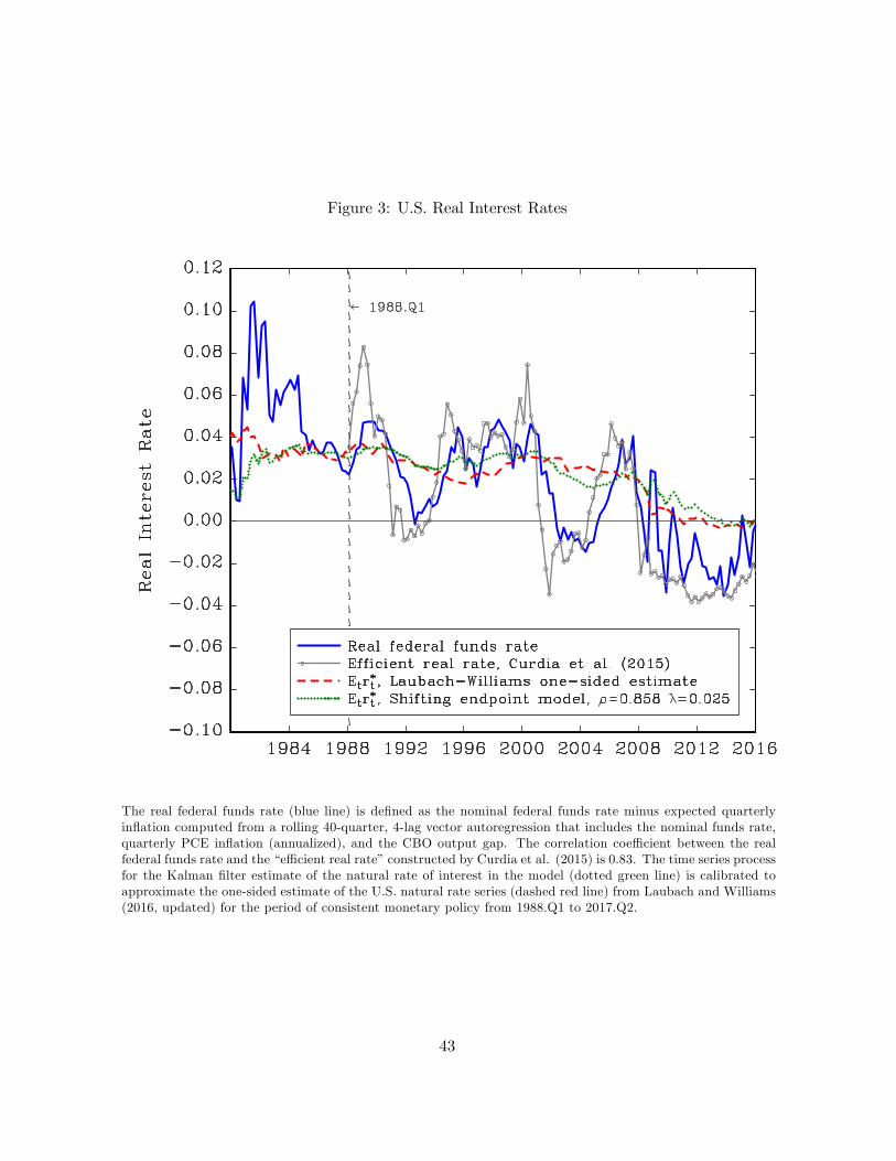
Figure 3: U.S. Real Interest Rates

The real federal funds rate (blue line) is defined as the nominal federal funds rate minus expected quarterlyinflation computed from a rolling 40-quarter, 4-lag vector autoregression that includes the nominal funds rate,quarterly PCE inflation (annualized), and the CBO output gap. The correlation coeffi cient between the realfederal funds rate and the “effi cient real rate”constructed by Curdia et al. (2015) is 0.83. The time series processfor the Kalman filter estimate of the natural rate of interest in the model (dotted green line) is calibrated toapproximate the one-sided estimate of the U.S. natural rate series (dashed red line) from Laubach and Williams(2016, updated) for the period of consistent monetary policy from 1988.Q1 to 2017.Q2.

43

Figure 4: U.S. Data

The real federal funds rate has remained mostly below the Laubach-Williams estimate of r∗t since early 2009.The nominal federal funds rate was approximately zero from 2008.Q4 through 2015.Q4. A Taylor-type rule ofthe form (11) using the parameter values in Table 2, with Etr∗t given by Laubach-Williams estimate, πt given bythe 4-quarter PCE inflation rate, and yt given by the CBO output gap predicts that the desired nominal fundsrate was negative starting in 2009.Q1 and remains negative through 2016.Q4. The 4-quarter PCE inflationrate was briefly negative in 2009 and has remained below the Fed’s 2% inflation target since 2012.Q2. TheGreat Recession was very severe, pushing the CBO output gap down to −6.3% at the business cycle trough in2009.Q2. The output gap remains negative at −0.2% in 2017.Q2, eight years after the Great Recession ended.The various endpoints plotted in the figure are computed using the expressions in Table 1, with r∗t given bythe Laubach-Williams estimate. As r∗t approaches zero or becomes negative, the “deflation” equilibrium ischaracterized by zero or low inflation, allowing this equilibrium to provide a better fit of recent U.S. inflationdata.

44

Figure 5: Measures of Expected U.S. Inflation

Market-based measures of expected inflation from zero coupon inflation swap contracts and Treasury InflationProtected Securities (TIPS) dropped sharply in 2008.Q4, coinciding with the start of the ZLB episode. Themarket-based measures remain below the Fed’s 2% inflation target at the end of the data sample. The median1-year expected inflation rate from the Survey of Professional Forecasters (SPF) dropped sharply in 2008.Q4and has recovered slowly to a level that is below its pre-recession range. The 10-year survey measure does notexhibit a sharp drop in 2008.Q4, but has since trended downward to a level that is below its pre-recession range.The Federal Reserve Bank of St. Louis’Price Pressures Measure (PPM) represents the probability that the4-quarter PCE inflation rate over the next year will exceed 2.5%. The PPM dropped sharply in 2008.Q4 and iscurrently hovering around a probability of 10%.

45

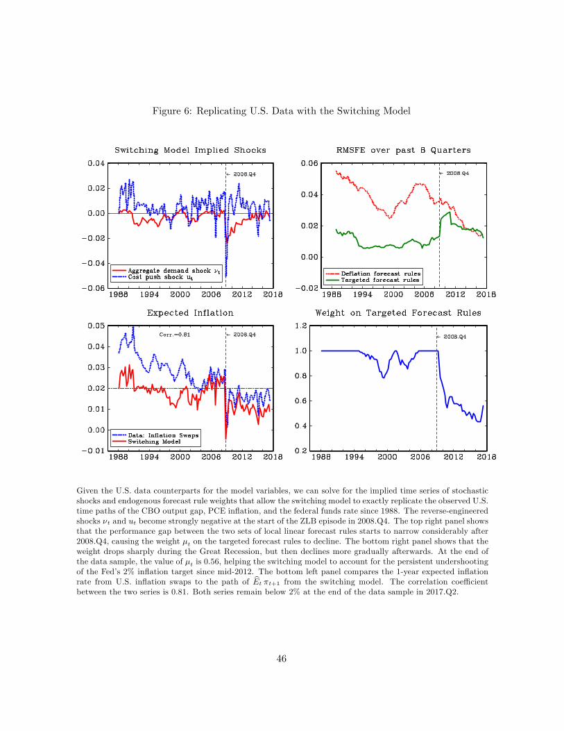
Figure 6: Replicating U.S. Data with the Switching Model

Given the U.S. data counterparts for the model variables, we can solve for the implied time series of stochasticshocks and endogenous forecast rule weights that allow the switching model to exactly replicate the observed U.S.time paths of the CBO output gap, PCE inflation, and the federal funds rate since 1988. The reverse-engineeredshocks νt and ut become strongly negative at the start of the ZLB episode in 2008.Q4. The top right panel showsthat the performance gap between the two sets of local linear forecast rules starts to narrow considerably after2008.Q4, causing the weight µt on the targeted forecast rules to decline. The bottom right panel shows that theweight drops sharply during the Great Recession, but then declines more gradually afterwards. At the end ofthe data sample, the value of µt is 0.56, helping the switching model to account for the persistent undershootingof the Fed’s 2% inflation target since mid-2012. The bottom left panel compares the 1-year expected inflationrate from U.S. inflation swaps to the path of Et πt+1 from the switching model. The correlation coeffi cientbetween the two series is 0.81. Both series remain below 2% at the end of the data sample in 2017.Q2.

46

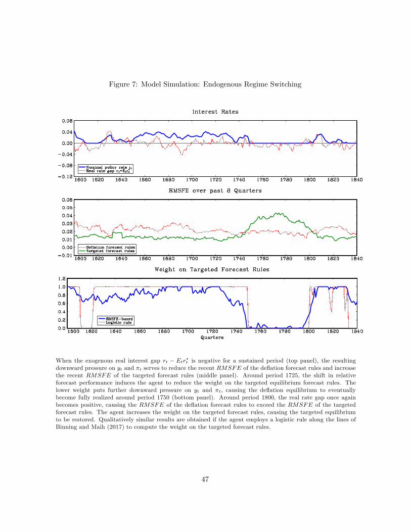
Figure 7: Model Simulation: Endogenous Regime Switching

When the exogenous real interest gap rt − Etr∗t is negative for a sustained period (top panel), the resultingdownward pressure on yt and πt serves to reduce the recent RMSFE of the deflation forecast rules and increasethe recent RMSFE of the targeted forecast rules (middle panel). Around period 1725, the shift in relativeforecast performance induces the agent to reduce the weight on the targeted equilibrium forecast rules. Thelower weight puts further downward pressure on yt and πt, causing the deflation equilibrium to eventuallybecome fully realized around period 1750 (bottom panel). Around period 1800, the real rate gap once againbecomes positive, causing the RMSFE of the deflation forecast rules to exceed the RMSFE of the targetedforecast rules. The agent increases the weight on the targeted forecast rules, causing the targeted equilibriumto be restored. Qualitatively similar results are obtained if the agent employs a logistic rule along the lines ofBinning and Maih (2017) to compute the weight on the targeted forecast rules.

47

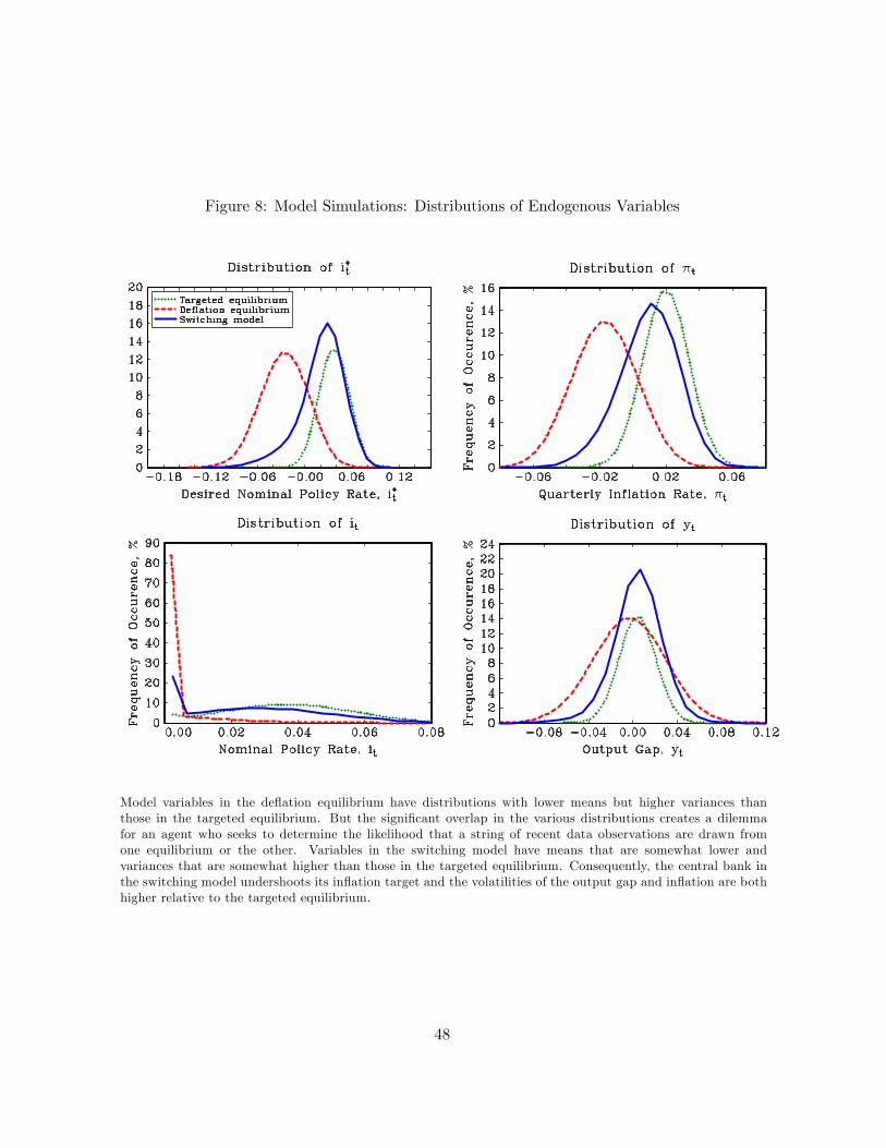
Figure 8: Model Simulations: Distributions of Endogenous Variables

Model variables in the deflation equilibrium have distributions with lower means but higher variances thanthose in the targeted equilibrium. But the significant overlap in the various distributions creates a dilemmafor an agent who seeks to determine the likelihood that a string of recent data observations are drawn fromone equilibrium or the other. Variables in the switching model have means that are somewhat lower andvariances that are somewhat higher than those in the targeted equilibrium. Consequently, the central bank inthe switching model undershoots its inflation target and the volatilities of the output gap and inflation are bothhigher relative to the targeted equilibrium.

48

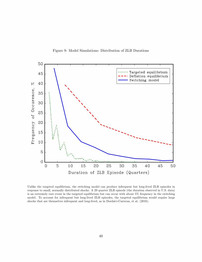
Figure 9: Model Simulations: Distribution of ZLB Durations

Unlike the targeted equilibrium, the switching model can produce infrequent but long-lived ZLB episodes inresponse to small, normally distributed shocks. A 29 quarter ZLB episode (the duration observed in U.S. data)is an extremely rare event in the targeted equilibrium but can occur with about 5% frequency in the switchingmodel. To account for infrequent but long-lived ZLB episodes, the targeted equilibrium would require largeshocks that are themselves infrequent and long-lived, as in Dordal-i-Carreras, et al. (2016).

49

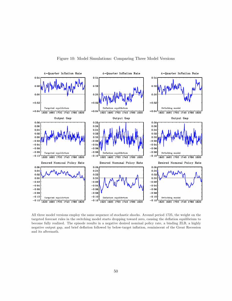
Figure 10: Model Simulations: Comparing Three Model Versions

All three model versions employ the same sequence of stochastic shocks. Around period 1725, the weight on thetargeted forecast rules in the switching model starts dropping toward zero, causing the deflation equilibrium tobecome fully realized. The episode results in a negative desired nominal policy rate, a binding ZLB, a highlynegative output gap, and brief deflation followed by below-target inflation, reminiscent of the Great Recessionand its aftermath.

50

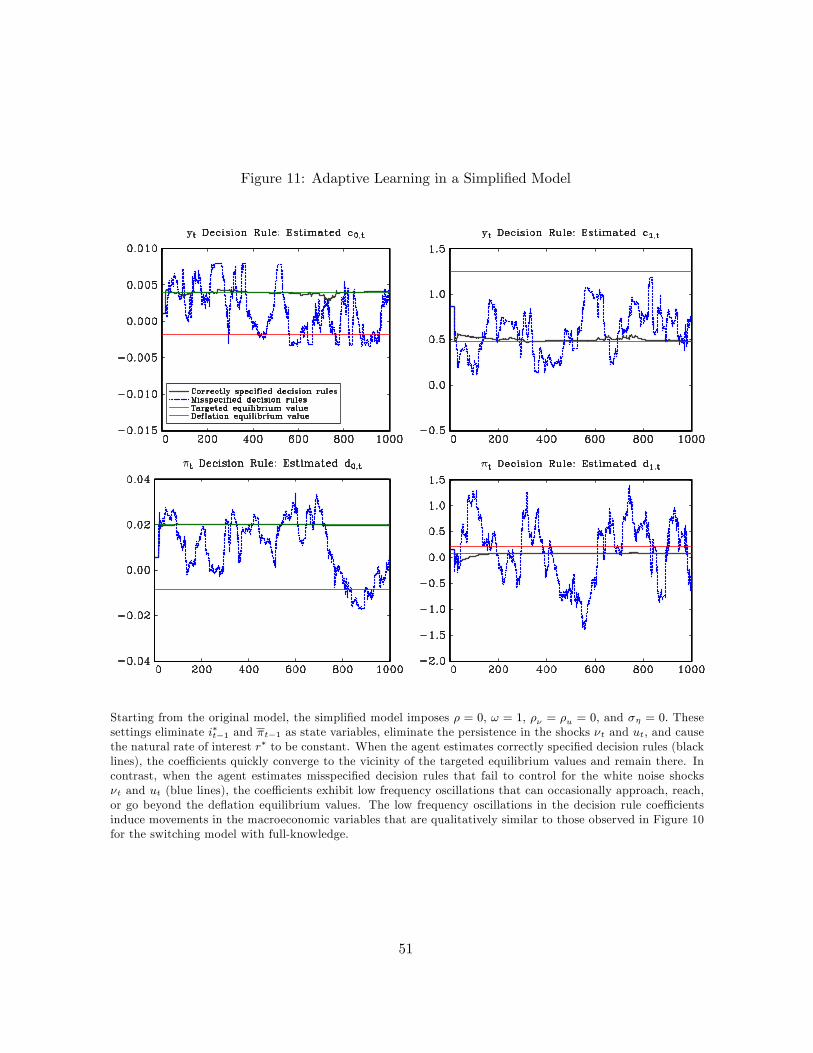
Figure 11: Adaptive Learning in a Simplified Model

Starting from the original model, the simplified model imposes ρ = 0, ω = 1, ρν = ρu = 0, and ση = 0. Thesesettings eliminate i∗t−1 and πt−1 as state variables, eliminate the persistence in the shocks νt and ut, and causethe natural rate of interest r∗ to be constant. When the agent estimates correctly specified decision rules (blacklines), the coeffi cients quickly converge to the vicinity of the targeted equilibrium values and remain there. Incontrast, when the agent estimates misspecified decision rules that fail to control for the white noise shocksνt and ut (blue lines), the coeffi cients exhibit low frequency oscillations that can occasionally approach, reach,or go beyond the deflation equilibrium values. The low frequency oscillations in the decision rule coeffi cientsinduce movements in the macroeconomic variables that are qualitatively similar to those observed in Figure 10for the switching model with full-knowledge.

51