ENDOGENOUS PRODUCTION NETWORKS AND

NON-LINEAR MONETARY TRANSMISSION ∗

Mishel Ghassibe†

University of Oxford

Abstract

I develop a tractable sticky-price model, where input-output linkages are formed endogenously.The model delivers cyclical properties of networks that are consistent with those I estimate usingsectoral and firm-level data, conditional on identified real and nominal shocks. A novel sourceof state dependence in nominal rigidities arises: whenever firms optimally choose to connect tomore suppliers, pricing complementarities and monetary non-neutrality strengthen, and vice versa.As a result, the model jointly rationalizes observed non-linearities associated with monetary trans-mission. First, the model produces cycle dependence: the magnitude of real GDP’s response to amonetary shock is procyclical. This occurs because in expansions the level of productivity is high,encouraging cost-minimizing firms to connect to more suppliers, which makes pricing decisionsmore co-ordinated and monetary non-neutrality stronger. Second, there is path dependence: non-neutrality of real GDP is higher following previous periods of loose monetary policy. The latterhappens as under nominal rigidities higher supply of money makes prices charged by supplierscheap relative to the cost of in-house labor, encouraging more connections and strengthening pricingcomplementarities. Third, there is size dependence: larger monetary expansions make the productionnetwork denser and hence have a disproportionally larger effect on GDP than smaller expansions;on the other hand, larger monetary contractions break the network and have a disproportionallysmaller effect. Such size dependence holds even under fully time-dependent pricing.

JEL Classification: C67, E23, E52.

Keywords: monetary transmission; state dependence; endogenous production networks.

∗First draft: February 2020; Current draft: October 11th 2021. I would like to thank Klaus Adam, Guido Ascari, Matteo Bizzarri(discussant), David Baqaee, Mihnea Constantinescu, Andrea Ferrero, Yuriy Gorodnichenko, Basile Grassi, Dominik Hecker (discus-sant), Jennifer La’O, Matthias Meier, Virgiliu Midrigan, Federica Romei, Raffaele Rossi, Solomiya Shpak, Jon Steinsson, FrancescoZanetti, participants of 2021 EEA-ESEM, 2021 Society for Economic Dynamics Annual Meeting, 2021 International Association forApplied Econometrics Annual Conference, 2021 Computing in Economics and Finance Conference, 2021 Cambridge INET NetworksConference, 1st NuCamp Virtual PhD Workshop, 1st Bocconi Virtual PhD Conference, 2020 European Winter Meeting of the Econo-metric Society, 14th RGS Doctoral Conference in Economics, as well as seminar attendees at the University of California-Berkeley,London School of Economics, Banque de France, University of Oxford, University of Manchester, National Bank of Ukraine andKyiv School of Economics for useful comments and suggestions. All errors and omissions are mine.†Department of Economics, University of Oxford, Manor Road Building, Oxford OX1 3UQ, United Kingdom;

mishel.ghassibe@economics.ox.ac.uk.

1 Introduction

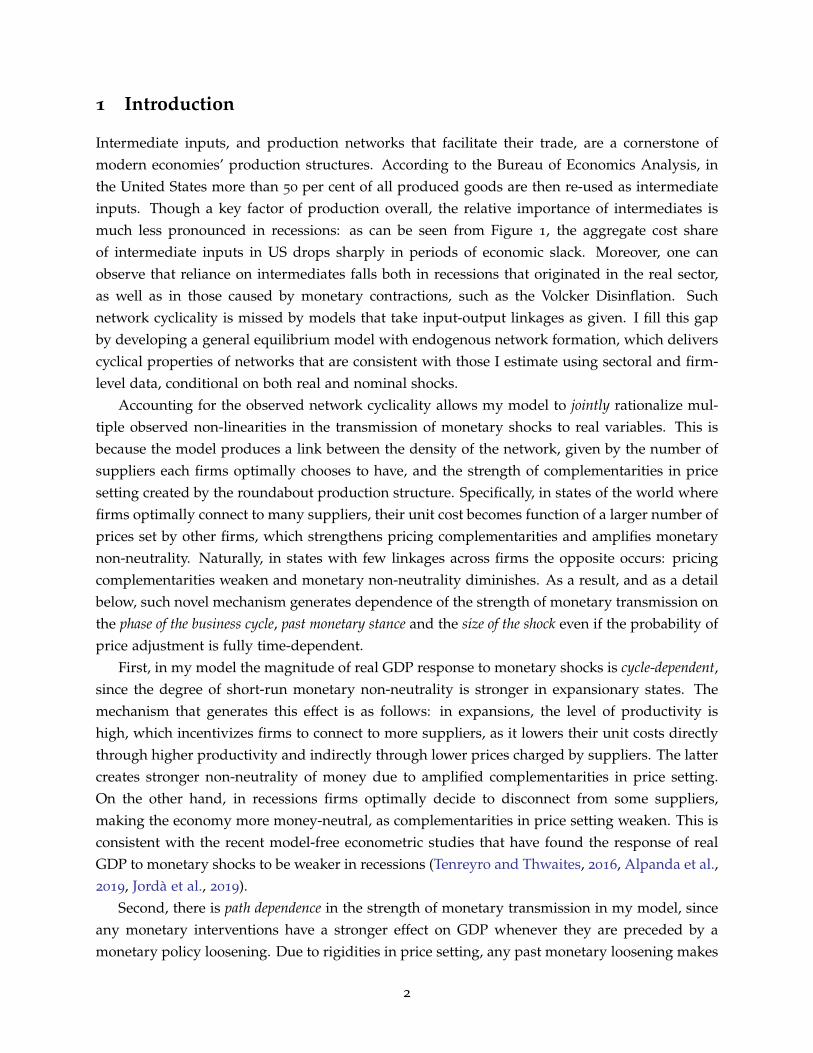
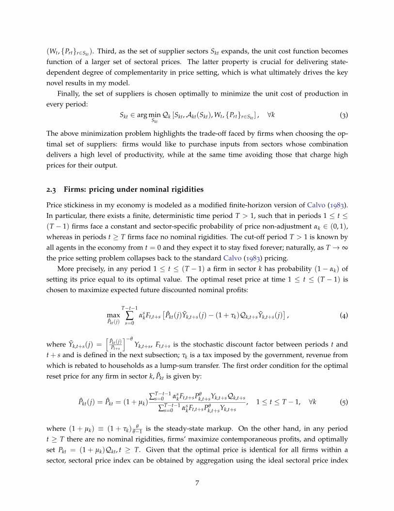
Intermediate inputs, and production networks that facilitate their trade, are a cornerstone ofmodern economies’ production structures. According to the Bureau of Economics Analysis, inthe United States more than 50 per cent of all produced goods are then re-used as intermediateinputs. Though a key factor of production overall, the relative importance of intermediates ismuch less pronounced in recessions: as can be seen from Figure 1, the aggregate cost shareof intermediate inputs in US drops sharply in periods of economic slack. Moreover, one canobserve that reliance on intermediates falls both in recessions that originated in the real sector,as well as in those caused by monetary contractions, such as the Volcker Disinflation. Suchnetwork cyclicality is missed by models that take input-output linkages as given. I fill this gapby developing a general equilibrium model with endogenous network formation, which deliverscyclical properties of networks that are consistent with those I estimate using sectoral and firm-level data, conditional on both real and nominal shocks.

Accounting for the observed network cyclicality allows my model to jointly rationalize mul-tiple observed non-linearities in the transmission of monetary shocks to real variables. This isbecause the model produces a link between the density of the network, given by the number ofsuppliers each firms optimally chooses to have, and the strength of complementarities in pricesetting created by the roundabout production structure. Specifically, in states of the world wherefirms optimally connect to many suppliers, their unit cost becomes function of a larger number ofprices set by other firms, which strengthens pricing complementarities and amplifies monetarynon-neutrality. Naturally, in states with few linkages across firms the opposite occurs: pricingcomplementarities weaken and monetary non-neutrality diminishes. As a result, and as a detailbelow, such novel mechanism generates dependence of the strength of monetary transmission onthe phase of the business cycle, past monetary stance and the size of the shock even if the probability ofprice adjustment is fully time-dependent.

First, in my model the magnitude of real GDP response to monetary shocks is cycle-dependent,since the degree of short-run monetary non-neutrality is stronger in expansionary states. Themechanism that generates this effect is as follows: in expansions, the level of productivity ishigh, which incentivizes firms to connect to more suppliers, as it lowers their unit costs directlythrough higher productivity and indirectly through lower prices charged by suppliers. The lattercreates stronger non-neutrality of money due to amplified complementarities in price setting.On the other hand, in recessions firms optimally decide to disconnect from some suppliers,making the economy more money-neutral, as complementarities in price setting weaken. This isconsistent with the recent model-free econometric studies that have found the response of realGDP to monetary shocks to be weaker in recessions (Tenreyro and Thwaites, 2016, Alpanda et al.,2019, Jorda et al., 2019).

Second, there is path dependence in the strength of monetary transmission in my model, sinceany monetary interventions have a stronger effect on GDP whenever they are preceded by amonetary policy loosening. Due to rigidities in price setting, any past monetary loosening makes

2

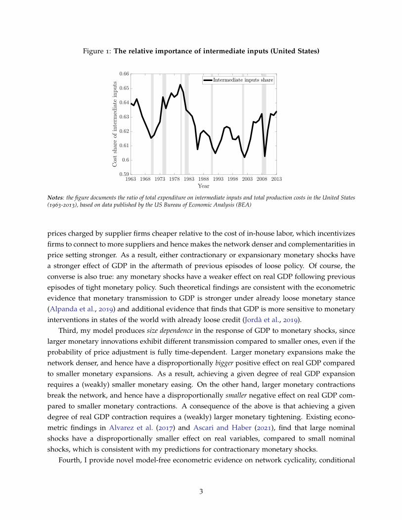
Figure 1: The relative importance of intermediate inputs (United States)

Notes: the figure documents the ratio of total expenditure on intermediate inputs and total production costs in the United States(1963-2013), based on data published by the US Bureau of Economic Analysis (BEA)

prices charged by supplier firms cheaper relative to the cost of in-house labor, which incentivizesfirms to connect to more suppliers and hence makes the network denser and complementarities inprice setting stronger. As a result, either contractionary or expansionary monetary shocks havea stronger effect of GDP in the aftermath of previous episodes of loose policy. Of course, theconverse is also true: any monetary shocks have a weaker effect on real GDP following previousepisodes of tight monetary policy. Such theoretical findings are consistent with the econometricevidence that monetary transmission to GDP is stronger under already loose monetary stance(Alpanda et al., 2019) and additional evidence that finds that GDP is more sensitive to monetaryinterventions in states of the world with already loose credit (Jorda et al., 2019).

Third, my model produces size dependence in the response of GDP to monetary shocks, sincelarger monetary innovations exhibit different transmission compared to smaller ones, even if theprobability of price adjustment is fully time-dependent. Larger monetary expansions make thenetwork denser, and hence have a disproportionally bigger positive effect on real GDP comparedto smaller monetary expansions. As a result, achieving a given degree of real GDP expansionrequires a (weakly) smaller monetary easing. On the other hand, larger monetary contractionsbreak the network, and hence have a disproportionally smaller negative effect on real GDP com-pared to smaller monetary contractions. A consequence of the above is that achieving a givendegree of real GDP contraction requires a (weakly) larger monetary tightening. Existing econo-metric findings in Alvarez et al. (2017) and Ascari and Haber (2021), find that large nominalshocks have a disproportionally smaller effect on real variables, compared to small nominalshocks, which is consistent with my predictions for contractionary monetary shocks.

Fourth, I provide novel model-free econometric evidence on network cyclicality, conditional

3

on identified productivity and monetary shocks, which supports the theoretical mechanism inmy model. As a first exercise, I use sectoral data from US Bureau of Economic Analysis (BEA)to construct annual time series of intermediates intensities for 65 sectors of the US economy.Consistent with the theoretical prediction, I find that intermediates intensity rises following apositive productivity shock, and following a monetary easing. Moreover, I find evidence thatthe effect is asymmetric: expansionary shocks, both productivity and monetary, lead to dispro-portionally larger magnitudes of network responses. I compare estimated responses with thosegenerated by a calibrated version of my model, and find them to be close, both in magnitudesand in the asymmetry of responses. One limitation of using sectoral data is that it does not allowto disentangle intensive and extensive margins of network adjustment, whereas it is the latterthat is predicted by my model. I therefore provide additional evidence using data on firm-levellinkages in Compustat, as constructed by Atalay et al. (2011). My findings using firm-level dataconfirm the evidence obtained using sectoral data, both in terms of directions of responses toproductivity and monetary shocks, and in terms of the asymmetries detected.

Contribution to the literature. This paper makes a contribution to three strands of the liter-ature. First, it contributes to the relatively recent literature on endogenous production networksin macroeconomics, by developing the first general equilibrium model featuring endogenousnetwork formation under nominal rigidities. It also provides novel model-free econometric ev-idence on network cyclicality, both unconditionally and conditional on productivity and mon-etary shocks, which the model successfully replicates. Previous macroeconomic studies havefocused on environments with flexible prices (Carvalho and Voigtlander, 2015; Oberfield, 2018;Acemoglu and Azar, 2020) or on finding the social planner’s solution to the network formationproblem (Taschereau-Dumouchel, 2019).

Second, it contributes to the literature on non-linearities in monetary transmission. In particu-lar, it develops a tractable framework that can jointly rationalize multiple non-linearities througha novel theoretical channel, which is shown to find support in both aggregate and disaggre-gated data. Therefore, although this is not the first paper to rationalize non-linearities in mon-etary transmission, it does so using a completely new mechanism. In prior literature, Santoroet al. (2014) study asymmetric transmission of monetary policy under loss aversion; McKay andWieland (2019) rationalize path dependence in a framework with lumpy durable consumptiondemand; Alpanda et al. (2019) explain non-linearities in a model with constraints on householdborrowing and refinancing; Eichenbaum et al. (2018) show how the effect on monetary policydepends on the distribution of savings from refinancing mortages; Berger et al. (2021) inves-tigate path-dependence under pre-payable mortgages; Bernstein (2021) shows that presence ofoccasionally binding borrowing constraints and household heterogeneity makes responses tomonetary transmission stronger in expansions and contractionary shocks more powerful thanexpansionary ones.

Third, the paper adds to the literature on monetary transmission in multi-sector New Keyne-sian models with roundabout production and asymmetric input-output linkages. Specifically, it

4

provides novel sector-level closed-form characterization of monetary transmission under endoge-nous network formation in a simplified version of the model, and develops a novel numericalalgorithm for finding sector-level solutions to a forward-looking version of the model with anarbitrary number of sectors. Previous studies quantify monetary transmission under fixed ex-ogenous production networks (Nakamura and Steinsson, 2010; Pasten et al., 2020; Ghassibe, 2021)or aim to explicitly estimate New Keynesian models with exogenous networks (Smets et al., 2019;Carvalho et al., 2021). As for optimal monetary policy under fixed exogenous networks, it hasbeen studied by La’O and Tahbaz-Salehi (2020) and Rubbo (2020).

The rest of the paper is structured as follows. Section 2 sets out the general theoreticalframework. Section 3 develops an analytically tractable version of the model and presents thekey theoretical results. Section 4 develops a numerical algorithm for solving a dynamic forwardlooking version of the model and quantifies the key effects. Section 5 presents novel econometricevidence that corroborates the key mechanisms of the model. Section 6 concludes.

2 A general theory formulation

My theory unifies two environments that have so far been treated as separate in the literature.On the one hand, my model features a multi-sector roundabout production structure, with firms’pricing subject to sector-specific nominal rigidities, in spirit of Pasten et al. (2020) and Ghassibe(2021), but without specifying functional forms. On the other hand, input-output linkages areformed endogenously by firms’ desire to optimize their production costs, in a manner introducedby Acemoglu and Azar (2020) in a static, flexible-price environment. As a result, the equilibriumproduction network responds to changes in real and monetary conditions, both realized andanticipated, allowing for the degree of complementarity in price setting to vary across states ofthe world. The latter is my key novel mechanism.

2.1 Model primitives

Time is discrete, with outcomes in t = 0 exogenously given, and outcomes in t ≥ 1 determined byagents’ decisions. There are three types of agents in my model. First, a continuum of infinitelylived households. Second, a continuum of monopolistically competitive firms, owned by thehouseholds, where each firm belongs to one, and only one, of the K sectors; let the set of allfirms in sector k be Φk, ∀k = 1, 2, ..., K. Third, a government, comprising of a central bank whichconducts monetary policy, and a fiscal authority which collects taxes from firms and rebates themto households.

A crucial feature of my economy is presence of a roundabout production structure across sec-tors, where the input-output linkages are formed endogenously through each firm’s choice of setof suppliers, denoted by Sk ⊆ 1, 2, ..., K, ∀k, ∀j ∈ Φk. For every choice of supplier sectors, thereis a given level of productivity pinned down by a predetermined time- and sector-specific map-

5

ping Akt(Skt)∞t=1, and At ≡ [A1t(.),A2t(.), ...,AKt(.)]′, ∀t. Importantly, the entire path At∞

t=1

is known to the agents at t = 0, and it is expected to remain unchanged forever. For any twomappings A and A, the convention is that A ≥ A if and only if Ak(Sk) ≥ Ak(Sk), ∀Sk, ∀k.

As for the nominal side of the economy, at t = 0 the agents know the initial level of moneysupplyM0, and expect it to remain unchanged forever. At the beginning of the first period t = 1,they discover the future path of money supply Mt∞

t=1, and there is no uncertainty from thereonwards. The central bank credibly commits to a set of policies that maintain the equilibriumquantity of money at the exogenous levelMt in every period t ≥ 1.

2.2 Firms: production and endogenous choice of suppliers

On the production side, there are K sectors, indexed by k = 1, 2, ..., K with a measure one of firmsin each sector; let Φk denote the set of all firms in sector k. The production function of firm j ∈ Φk

is given by:Ykt(j) = Fk

[Skt,Akt(Skt), Nkt(j), Zkrt(j)r∈Skt

](1)

where Skt ⊆ 1, 2, ..., K is the set of sectors, whose firms supply inputs to firms in sector k attime t, Akt(.) is a mapping from the chosen set of suppliers to the associated level of productivityat time t, Nkt(j) is the labor input of firm j in sector k at time t, whereas Zkrt(j) denotes purchasesof intermediate inputs from sector r, which is in turn is an aggregator of purchases from all

firms in that sector: Zkrt(j) ≡(∫

j′∈ΦrZkrt(j, j′)

θ−1θ dj′

) θθ−1

, θ > 1. I impose the following regularityconditions on the production function:

Assumption 1 (Production function). For every sector k = 1, 2, ..., K, the production function sat-

isfies the following conditions: (a) Fk is strictly quasi-concave, exhibits constant returns to scale in

(Nkt(j), Zkrt(j)r∈Skt), is increasing and continuous in Akt(Skt), Nkt(j) and Zkrt(j)r∈Skt

, and is

strictly increasing in Akt(Skt) when Nkt(j) > 0 and Zkrt(j)r∈Skt> 0; (b) labor is an essential fac-

tor of production: Fk(·, ·, 0, ·) = 0; (c) Akt(∅) > 0.

Conditional on a particular set of suppliers Skt, each firm’s total cost of production at time tis given by

[WtNkt(j) + ∑r∈Skt

PrtZkrt(j)], where Wt is the nominal wage and Prt is price index of

sector r. Taking as given Skt, Wt and Prtr∈Skt , each firm chooses labor and intermediate inputquantities to minimize the total cost, subject to the production function in (1). The latter deliversthe following unit cost function:

Qkt(j) = Qk [Skt,Akt(Skt), Wt, Prtr∈Skt ] . (2)

Three properties of the unit cost function should be noted. First, the unit cost function is commonfor all firms within a given sector. Second, given the properties of the production function, Qk

is decreasing and continuous in Akt(Skt) and is increasing and homogenous of degree one in

6

(Wt, Prtr∈Skt). Third, as the set of supplier sectors Skt expands, the unit cost function becomesfunction of a larger set of sectoral prices. The latter property is crucial for delivering state-dependent degree of complementarity in price setting, which is what ultimately drives the keynovel results in my model.

Finally, the set of suppliers is chosen optimally to minimize the unit cost of production inevery period:

Skt ∈ arg minSktQk [Skt,Akt(Skt), Wt, Prtr∈Skt ] , ∀k (3)

The above minimization problem highlights the trade-off faced by firms when choosing the op-timal set of suppliers: firms would like to purchase inputs from sectors whose combinationdelivers a high level of productivity, while at the same time avoiding those that charge highprices for their output.

2.3 Firms: pricing under nominal rigidities

Price stickiness in my economy is modeled as a modified finite-horizon version of Calvo (1983).In particular, there exists a finite, deterministic time period T > 1, such that in periods 1 ≤ t ≤(T − 1) firms face a constant and sector-specific probability of price non-adjustment αk ∈ (0, 1),whereas in periods t ≥ T firms face no nominal rigidities. The cut-off period T > 1 is known byall agents in the economy from t = 0 and they expect it to stay fixed forever; naturally, as T → ∞the price setting problem collapses back to the standard Calvo (1983) pricing.

More precisely, in any period 1 ≤ t ≤ (T − 1) a firm in sector k has probability (1− αk) ofsetting its price equal to its optimal value. The optimal reset price at time 1 ≤ t ≤ (T − 1) ischosen to maximize expected future discounted nominal profits:

maxPkt(j)

T−t−1

∑s=0

αskFt,t+s

[Pkt(j)Yk,t+s(j)− (1 + τk)Qk,t+sYk,t+s(j)

], (4)

where Yk,t+s(j) =[

Pkt(j)Pt+s

]−θYk,t+s, Ft,t+s is the stochastic discount factor between periods t and

t + s and is defined in the next subsection; τk is a tax imposed by the government, revenue fromwhich is rebated to households as a lump-sum transfer. The first order condition for the optimalreset price for any firm in sector k, Pkt is given by:

Pkt(j) = Pkt = (1 + µk)∑T−t−1

s=0 αskFt,t+sPθ

k,t+sYk,t+sQk,t+s

∑T−t−1s=0 αs

kFt,t+sPθk,t+sYk,t+s

, 1 ≤ t ≤ T − 1, ∀k (5)

where (1 + µk) ≡ (1 + τk)θ

θ−1 is the steady-state markup. On the other hand, in any periodt ≥ T there are no nominal rigidities, firms’ maximize contemporaneous profits, and optimallyset Pkt = (1 + µk)Qkt, t ≥ T. Given that the optimal price is identical for all firms within asector, sectoral price index can be obtained by aggregation using the ideal sectoral price index

7

Pkt ≡(∫

j∈ΦkPkt(j)1−θdj

) 11−θ

, ∀k:

Pkt =

[αkP1−θ

k,t−1 + (1− αk)(Pkt)1−θ] 1

1−θ, 1 ≤ t ≤ (T − 1);

(1 + µk)Qkt, t ≥ T.

(6)

I use such modified version of Calvo (1983) pricing for two reasons. First, the special case whereT = 2 is analytically tractable at the sector-level, as I show in Section 3. Second, given thatmoney is neutral for all t ≥ T, such formulation of pricing allows to obtain a numerical sector-level solution for the forward-looking problem with endogenous network formation at t < T bybackward induction, as is performed in Section 4.

2.4 Households

A continuum of infinitely lived households populates my economy and owns all the firms. Mar-kets are complete, and a full set of Arrow-Debreu securities is available. The representativehousehold makes choices to maximize the lifetime utility:

maxCt+s,Nt+s,Bt+s+1∞

s=0

∞

∑s=0

βs [ln Ct+s − Nt+s] (7)

subject to

Pct Ct + [Ft,t+1Bt+1] ≤ Bt + WtNt +

K

∑k=1

Πkt + Tt, ∀t (8)

where Ct is aggregate consumption, Pct is consumption price index (defined below), Nt is labor

supply, Bt+1 is the payoff of securities purchased at time t, Ft,t+1 is the price of those securitiesat time t, Πkt denotes aggregate nominal profits of firms in sector k, β is the discount factor forfuture utility and Tt are lump-sum transfers from the government.1

The households’ maximization problem yields standard aggregate first-order conditions,

namely an equation for the stochastic discount factor Ft,t+s = βs(

Ct+sCt

)−1 Pct

Pct+s

, and the labor

supply equation C−1t =

Pct

Wt.

The composite consumption index Ct is an aggregator for the final consumption of goodsproduced in the different sectors of my economy:

Ct ≡ u(C1t, C2t, ..., CKt), (9)

1The assumption of log utility of consumption and linear disutility of labor follows the indivisible labor modelintroduced by Hansen (1985). Such formulation is made for analytical tractability and is the baseline choice in otherworkhorse models of monetary policy and production networks, such as Nakamura and Steinsson (2010).

8

where Ckt is in turn an aggregator for the final consumption of goods produced by firms in

that sector: Ckt ≡(∫

j∈ΦrCkt(j)

θ−1θ dj

) θθ−1

, ∀k. I impose the following regularity conditions on theaggregator u:

Assumption 2 (Consumption aggregation). The consumption aggregator u is continuous, differen-

tiable, increasing, strictly quasi-concave and homogeneous of degree one in (C1t, C2t, ..., CKt), and all

sectoral consumption goods are normal.

Households choose their sectoral consumption levels by minimizing the total cost of pur-chases ∑K

k=1 PktCkt subject to the consumption aggregator in (9). The latter also delivers theconsumption price index Pc

t = Pct (P1t, P2t, ..., PKt), as the minimal cost of assembling such a bas-

ket.

2.5 Monetary policy

Purchases of final goods are subject to a cash-in-advance constraint, so that Pct Ct =Mt, ∀t ≥ 1.

Agents are aware of the initial level of money supply M0, and at t = 0 anticipate it to stay atthat level forever. In period t = 1 they discover the future path of money supply Mt∞

t=1 andtherefore any Mt 6=M0 constitutes a monetary shock at time t to the agents. I assume that thecentral bank makes a credible commitment at t = 1 to ensure the equilibrium quantity of moneyfollows the exogenous path Mt∞

t=1.

2.6 Market clearing and equilibrium

In addition to the optimality conditions, budget constraints and the policy rule above, equi-librium in my economy is characterized by market-clearing conditions in the asset market:Bt = 0; the the labor market: Nt = ∑K

k=1∫

j∈ΦkNkt(j)dj; and the goods markets: Ykt(j) =

Ckt(j) + ∑Kr=1∫

j′∈ΦrZrkt(j′, j)dj′, ∀k, ∀j ∈ Φk. All in all, equilibrium in my economy can be

summarized as follows:

Definition 1 (Equilibrium). Equilibrium is a collection of prices Pkt(j)|j ∈ ΦkKk=1, wage Wt, allo-

cations

Ykt(j), Nkt(j), Ckt(j), Zkrt(j, j′)|j′ ∈ ΦrKr=1 |j ∈ Φk

K

k=1and supplier choices SktK

k=1, which

given the exogenous path of productivity mapping At∞t=1, the exogenous series of money supply Mt∞

t=0

and the exogenous initial prices Pk0Kk=1, satisfy agent optimization and market clearing in every time

period t ≥ 1.

3 An analytically tractable version

In this section I consider an analytically tractable version of the model obtained when nominalrigidities are only present in the first period. Such simplification allows to formally character-

9

ize propagation of monetary shocks to real variables, under different states of productivity andinitial levels of money supply. Formal propositions establish that small monetary shocks, whichdo not affect the shape of the network, have an impact on GDP that is larger whenever produc-tivity mapping improves or initial money supply rises. Further, large monetary expansions havemore than proportional positive effect on GDP than small monetary expansions; on the otherhand, large monetary contractions have less than proportional negative effect on GDP than smallmonetary contractions. All proofs are given in Appendix A.

3.1 Equilibrium in the simplified version

In this section I focus on the version of my model with T = 2, so that nominal rigidities areonly present at t = 1. In particular, I show that such simplification allows to both formallyestablish equilibrium existence and uniqueness properties, as well as to analytically characterizetransmission of monetary shocks under different baseline productivity mappings and levels ofmoney supply. The assumption is formally documented below:

Assumption 3 (Horizon of stickiness). In the firms’ pricing problem T = 2, so that nominal rigidities

are only present at t = 1, and prices are fully flexible for all t ≥ 2.

One implication of the above assumption is that the optimal reset price at t = 1 is deter-mined by Pk1 = (1 + µk)Qk1, ∀k, delivering a tractable expression for the sectoral price index in

the first period, namely Pk1 =[αkP1−θ

k0 + (1− αk) (1 + µk)Qk11−θ] 1

1−θ, ∀k. At the same time,

prices are flexible after the first period, so that Pkt = (1 + µk)Qkt, ∀k, t ≥ 2. Moreover, noticethat the intratemporal consumption-labor supply condition and the cash-in-advance constraintjointly imply that Wt = Mt, so that the nominal wage equals money supply in every period. Thisexogeneity of the nominal wage, combined with the fact that the only endogenous component inthe pricing equations above is the unit cost function, jointly imply that prices in this simplifiedsetting are pinned down exclusively by the exogenous supply-side factors – productivity map-ping At and markups µkK

k=1 – and by the exogenous level of money supply. It is the latterproperty which allows to represent equilibrium sectoral prices as a lattice, which in turn deliversequilibrium existence and uniqueness properties summarized below.

Proposition 1 (Equilibrium). Suppose Assumptions 1-3 hold. Then the equilibrium introduced in Defi-

nition 1 entails the following properties: (a) it exists; (b) the equilibrium sectoral prices and final sectoral

consumptions are unique; (c) the equilibrium supplier choices and remaining sectoral allocations are gener-

ically unique.

Since Assumption 3 implies that money is neutral for t ≥ 2 and given that my interest isin the transmission of monetary shocks to real variables, in the rest of this section I am goingto focus exclusively on outcomes at t = 1. For notational simplicity, I drop time subscripts forvariables at t = 1 for the remainder of this section.

10

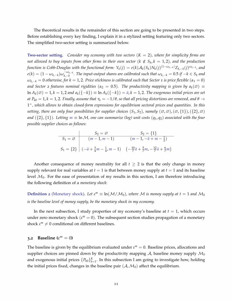
The theoretical results in the remainder of this section are going to be presented in two steps.Before establishing every key finding, I explain it in a stylized setting featuring only two sectors.The simplified two-sector setting is summarized below.

Two-sector setting. Consider my economy with two sectors (K = 2), where for simplicity firms arenot allowed to buy inputs from other firms in their own sector (k /∈ Sk, k = 1, 2), and the productionfunction is Cobb-Douglas with the functional form: Yk(j) = e(k)Ak(Sk)Nk(j)(1−ωk,−k)Zk,−k(j)ωk,−k , ande(k) = (1−ωk,−k)ω

−ωk,−kk,−k . The input-output shares are calibrated such that ωk,−k = 0.5 if −k ∈ Sk and

ωk,−k = 0 otherwise, for k = 1, 2. Price stickiness is calibrated such that Sector 1 is price flexible (α1 = 0)and Sector 2 features nominal rigidities (α2 = 0.5). The productivity mapping is given by ak(∅) ≡ln Ak(∅) = 1, k = 1, 2 and ak(−k) ≡ ln Ak(−k) = a, k = 1, 2. The exogenous initial prices are setat Pk0 = 1, k = 1, 2. Finally, assume that τk = −1/θ, so that all pricing distortions are removed, and θ →1+, which allows to obtain closed-form expressions for equilibrium sectoral prices and quantities. In thissetting, there are only four possibilities for supplier choices (S1, S2), namely (∅,∅), (∅, 1), (2,∅)

and (2, 1). Letting m ≡ lnM, one can summarize (log) unit costs (q1, q2) associated with the fourpossible supplier choices as follows:

S2 = ∅ S2 = 1S1 = ∅ (m− 1, m− 1) (m− 1,−a + m− 1

2 )

S1 = 2 (−a + 34 m− 1

4 , m− 1)(− 10

7 a + 57 m,− 12

7 a + 67 m)

Another consequence of money neutrality for all t ≥ 2 is that the only change in moneysupply relevant for real variables at t = 1 is that between money supply at t = 1 and its baselinelevel M0. For the ease of presentation of my results in this section, I am therefore introducingthe following definition of a monetary shock:

Definition 2 (Monetary shock). Let εm ≡ ln(M/M0), whereM is money supply at t = 1 andM0

is the baseline level of money supply, be the monetary shock in my economy.

In the next subsection, I study properties of my economy’s baseline at t = 1, which occursunder zero monetary shock (εm = 0). The subsequent section studies propagation of a monetaryshock εm 6= 0 conditional on different baselines.

3.2 Baseline (εm = 0)

The baseline is given by the equilibrium evaluated under εm = 0. Baseline prices, allocations andsupplier choices are pinned down by the productivity mapping A, baseline money supply M0

and exogenous initial prices Pk0Kk=1. In this subsection I am going to investigate how, holding

the initial prices fixed, changes in the baseline pair (A,M0) affect the equilibrium.

11

First, I am going to use the two-sector setting introduced earlier to build intuition on howchanges in the productivity mapping affect the baseline, ceteris paribus.

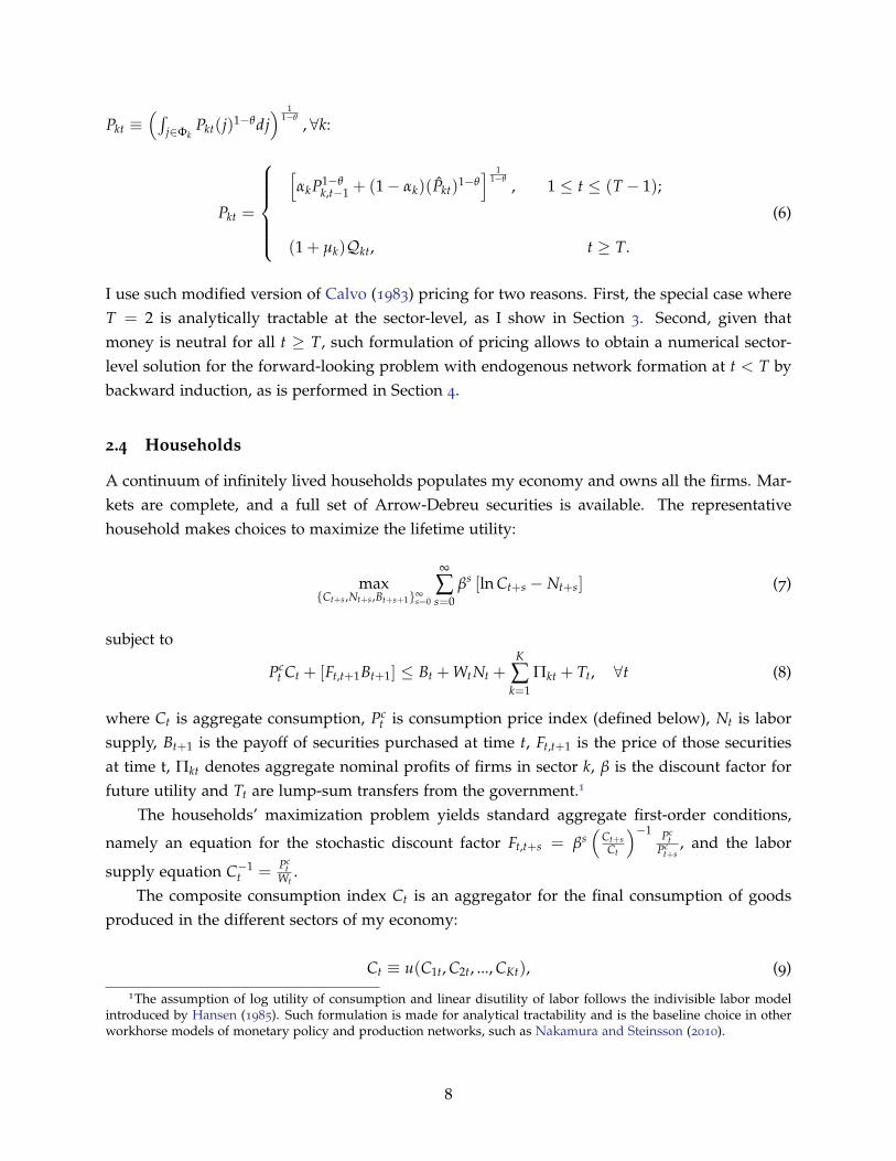
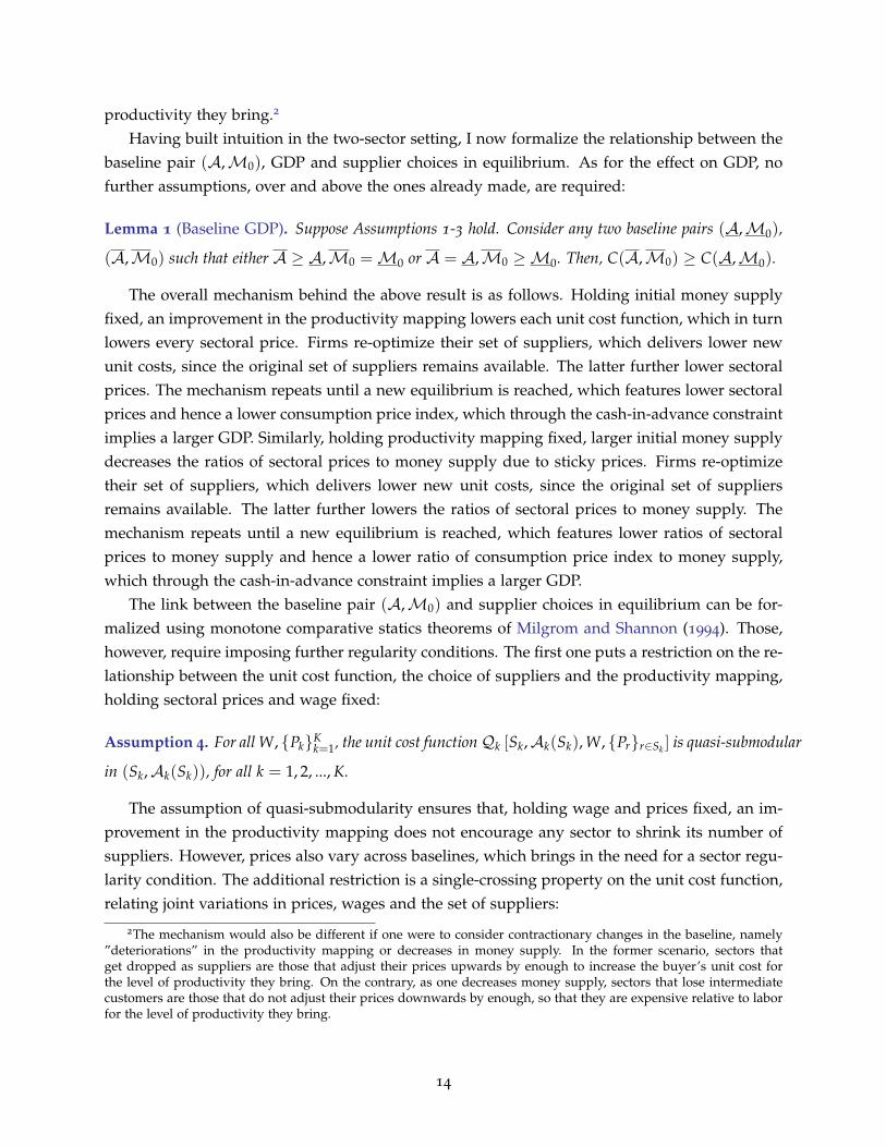
Example 1 (Productivity mapping and baseline). In Panel (a) of Figure 2 I use the two-sector settingwhere, holding baseline money supply fixed at m0 = 0, I consider three different productivity mappingsby varying the parameter a, which represents the productivity associated with using the other sector asa supplier. When a = 0, neither sector finds it optimal to buy inputs from the other sector, and theequilibrium network is empty. As I increase a to 0.65, the sticky-price Sector 2 finds it optimal to purchaseinputs from the flexible-price Sector 1, but not vice versa. This is because Sector 2 finds it optimal to lowerits unit cost by purchasing inputs from Sector 1, whose price flexibility is associated with lower prices.Finally, as I further increase a to 0.8, both sectors find it optimal to connect to each other. This is becausethe productivity associated with the connection is now sufficiently high to convince the flexible-price Sector1 to purchase from Sector 2, whose price stickiness prevents it from fully lowering the price. In addition,notice that as I increase the productivity parameter, equilibrium unit costs and hence sectoral prices drop,which lowers the consumption price index and through the cash-in-advance constraint implies that baselineGDP rises.

I now use the two-sector setting to build intuition on the link between initial money supplyand baseline equilibrium:

Example 2 (Money supply and baseline). In Panel (b) of Figure 2 I use the two-sector setting where,holding productivity mapping fixed at a = 0, I consider three different initial money supplies by varyingthe parameter m0. When m0 = 0, neither sector finds it optimal to buy inputs from the other sector, and theequilibrium network is empty. As I increase m0 to 4, the flexible-price Sector 1 finds it optimal to purchaseinputs from the sticky-price Sector 2, but not vice versa. This is because the nominal wage rises one-for-one with money supply, and Sector 1 finds it cheaper to substitute in-house labor for inputs bought fromSector 2, whose price increases less than one-for-one, even though such connection lowers 1’s productivity.Finally, as I further increase m0 to 8, both sectors find it optimal to connect to each other. This is becausethe increase in money supply/nominal wage is now so large that even the sticky-price Sector 2 wishes tosubstitute its in-house labor for inputs from Sector 1, whose price now does not track money supply sinceit inherits price stickiness from Sector 2, even though such connection lowers 2’s productivity. In addition,notice that as I increase money supply, the gap between money supply and equilibrium unit costs andprices, both sectoral and the aggregate consumption index, is growing, which through the cash-in-advanceconstraint implies that baseline GDP rises.

Therefore, in my simple examples, baseline GDP and the number of suppliers of each sector(weakly) rise, ceteris paribus, both as one improves the productivity mapping and as one increasesinitial money supply. However, the mechanisms through which linkages are added are, in fact,diagonally opposite under the two scenarios. As one improves the productivity mapping, extrasectors that get adopted as suppliers are those that adjust their prices downwards by enoughto lower the buyer’s unit cost for the level of productivity they bring. On the contrary, as oneincreases money supply, sectors that receive additional intermediate customers are those that donot adjust their prices upwards enough, so that they are cheaper relative to labor for the level of

12

Figure 2: Equilibrium supplier choices under different baseline conditions (two sectors)

(a) Equilibrium choices of suppliers under different baseline productivity mappings (m0 = 0)

Recession: a = 0

∅∅∅ 1∅∅∅ (-1,-1)

(−1,− 1

2

)2

(− 1

4 ,−1)

(0, 0)

Normal: a = 0.65

∅ 1∅∅∅ (−1,−1)

(−1,− 23

20)

2(− 9

10 ,−1) (

− 1314 ,− 39

35

)

Expansion: a = 0.80

∅ 1∅ (−1,−1) (−1,− 13

10 )

2(− 21

20 ,−1) (

− 87 ,− 48

35

)

(b) Equilibrium choices of suppliers under different baseline levels of money supply (a = 0)

Tight money: m0 = 0

∅∅∅ 1∅∅∅ (-1,-1)

(−1,− 1

2

)2

(− 1

4 ,−1)

(0, 0)

Normal money: m0 = 4

∅∅∅ 1∅ (3, 3)

(3, 5

2

)2

(114 , 3

) (207 , 24

7

)

Loose money: m0 = 8

∅ 1∅ (7, 7)

(7, 13

2

)2

(234 , 7

) (407 , 48

7

)

Notes: the figure uses the analytically tractable version of my model under T = 2, calibrated for K = 2, ωkk = 0, ∀k, Yk(j) =e(k)Ak(Sk)Nk(j)(1−ωk,−k)Zk,−k(j)ωk,−k and e(k) = (1−ωk,−k)ω

−ωk,−kk,−k , ak,0 ≡ logAk,0, ∀k and m0 = logM0, the production

technology be given by a1,0(∅) = 0, a1,0(2) = a, a2,0(∅) = 0, a2,0(1) = a, P10 = P20 = 1, the sectoral shares aregiven by ω12 = ωc1 = 0.5 = ω21 = ωc1 = 0.5, and Calvo parameters by α1 = 0, α2 = 0.5. Finally, assume that τk = −1/θ,and θ → 1+.

13

productivity they bring.2

Having built intuition in the two-sector setting, I now formalize the relationship between thebaseline pair (A,M0), GDP and supplier choices in equilibrium. As for the effect on GDP, nofurther assumptions, over and above the ones already made, are required:

Lemma 1 (Baseline GDP). Suppose Assumptions 1-3 hold. Consider any two baseline pairs (A,M0),

(A,M0) such that either A ≥ A,M0 =M0 or A = A,M0 ≥M0. Then, C(A,M0) ≥ C(A,M0).

The overall mechanism behind the above result is as follows. Holding initial money supplyfixed, an improvement in the productivity mapping lowers each unit cost function, which in turnlowers every sectoral price. Firms re-optimize their set of suppliers, which delivers lower newunit costs, since the original set of suppliers remains available. The latter further lower sectoralprices. The mechanism repeats until a new equilibrium is reached, which features lower sectoralprices and hence a lower consumption price index, which through the cash-in-advance constraintimplies a larger GDP. Similarly, holding productivity mapping fixed, larger initial money supplydecreases the ratios of sectoral prices to money supply due to sticky prices. Firms re-optimizetheir set of suppliers, which delivers lower new unit costs, since the original set of suppliersremains available. The latter further lowers the ratios of sectoral prices to money supply. Themechanism repeats until a new equilibrium is reached, which features lower ratios of sectoralprices to money supply and hence a lower ratio of consumption price index to money supply,which through the cash-in-advance constraint implies a larger GDP.

The link between the baseline pair (A,M0) and supplier choices in equilibrium can be for-malized using monotone comparative statics theorems of Milgrom and Shannon (1994). Those,however, require imposing further regularity conditions. The first one puts a restriction on the re-lationship between the unit cost function, the choice of suppliers and the productivity mapping,holding sectoral prices and wage fixed:

Assumption 4. For all W, PkKk=1, the unit cost functionQk [Sk,Ak(Sk), W, Prr∈Sk ] is quasi-submodular

in (Sk,Ak(Sk)), for all k = 1, 2, ..., K.

The assumption of quasi-submodularity ensures that, holding wage and prices fixed, an im-provement in the productivity mapping does not encourage any sector to shrink its number ofsuppliers. However, prices also vary across baselines, which brings in the need for a sector regu-larity condition. The additional restriction is a single-crossing property on the unit cost function,relating joint variations in prices, wages and the set of suppliers:

2The mechanism would also be different if one were to consider contractionary changes in the baseline, namely”deteriorations” in the productivity mapping or decreases in money supply. In the former scenario, sectors thatget dropped as suppliers are those that adjust their prices upwards by enough to increase the buyer’s unit cost forthe level of productivity they bring. On the contrary, as one decreases money supply, sectors that lose intermediatecustomers are those that do not adjust their prices downwards by enough, so that they are expensive relative to laborfor the level of productivity they bring.

14

Assumption 5. Let Qk[Sk,Ak(Sk), Prr∈Sk

]≡ 1

WQk

[Sk,Ak(Sk), 1, Pr

W r∈Sk

], ∀k. For all Sk ⊆ S

′k

and for all Pr, P′rKr=1 such that P′r ≤ Pr, ∀r 6= k:

Qk

[S′k,Ak(S′k), Prr∈S′k

]−Qk

[Sk,Ak(Sk), Prr∈Sk

]≤ 0

=⇒ Qk

[S′k,Ak(S′k), P′rr∈S′k

]−Qk

[Sk,Ak(Sk), P′rr∈Sk

]≤ 0, ∀k. (10)

The above single crossing property ensures that a reduction in all sectoral price to wageratios does not discourage the adoption of a larger number of suppliers by every sector. Such anassumption immediately holds under a range of widely used production functions, most notablyCobb-Douglas with Hicks-neutral technology.3

The additional assumptions above allow to formalize the link between the baseline pair(A,M0) and supplier choices in equilibrium:

Lemma 2 (Baseline supplier choices). Suppose Assumptions 1-5 hold. Consider any two baseline pairs

(A,M0), (A,M0) such that either A ≥ A,M0 =M0 or A = A,M0 ≥ M0. Then, Sk(A,M0) ⊇

Sk(A,M0), for all k = 1, 2, ..., K.

The intuition behind the above result is as follows. An improvement in the productivity map-ping, ceteris paribus, incentivizes firms to connect to more suppliers, as it lowers their unit costsdirectly through higher productivity and indirectly through lower prices charged by suppliers.Similarly, an increase in initial money supply, ceteris paribus, leads to a reduction in sectoral priceto wage ratios, implying that it is cost-reducing to substitute in-house labor for intermediatesbought from other sectors, thus leading to an increase in the number of suppliers.

3.3 Propagation of a monetary shock

Having established properties of the baseline, I now consider deviations from the baseline, drivenby a monetary shock εm. The mechanics of a monetary shock in terms of its effect on the equi-librium allocations and supplier choices are isomorphic to those for changes in baseline moneysupply established in the previous subsection. I can therefore immediately formalize comparativestatics following a monetary shock

Lemma 3 (Comparative statics following a monetary shock). Consider a baseline pair (A,M0),

which is perturbed by a monetary shock εm > 0. Suppose Assumptions 1-3 hold, then following the

monetary shock equilibrium GDP rises (falls) relative to its baseline level: C(A,M) > C(A,M0).

Further, suppose that in addition Assumption 4-5 also hold, then following the monetary shock the set of

suppliers for each sector weakly expands: Sk(A,M) ⊇ Sk(A,M0), for all k = 1, 2, ..., K.3This is formally shown in Acemoglu and Azar (2020). See their work for a fuller characterization of families of

production functions under which the single-crossing property in Assumption 5 holds.

15

Note that although the above lemma is stated for an expansionary monetary shock εm > 0,it naturally extends to a contractionary shock εm < 0, which leads to a reduction in GDP and aweak fall in the number of supplier for every sector.

From Lemma 3 it follows that a non-zero monetary shock can either change the set of sup-pliers relative to the baseline, or leave them unchanged. In light of this it is useful to formallydistinguish between two such types of monetary shocks, as is done below.

Definition 3 (Small monetary shock). Define a monetary shock εm to be small with respect to the

baseline (A,M0) if and only if it leaves the equilibrium supplier choices unchanged for all sectors relative

to the baseline: Sk(A,M) = Sk(A,M0), ∀k. Otherwise, define the monetary shock to be large with

respect to the baseline (A,M0).

Crucially, the above definition helps classify every monetary shock as either small or largewith respect to a specific baseline pair (A,M0). In principle, as one changes the baseline pair, ashock of a given size can switch from being small to large, or vice versa. Moreover, the definitionis not symmetric: for a given baseline, an expansionary shock εm > 0 being small does notnecessarily imply that a contractionary shock of an equal absolute value is small with respect tothe same baseline.

3.3.1 Small monetary shocks

In this section I study how responses of prices and allocations to a small monetary shock dependon the baseline productivity mapping and initial money supply. As before, I begin by buildingintuition in the simplified two-sector setting before establishing general results.

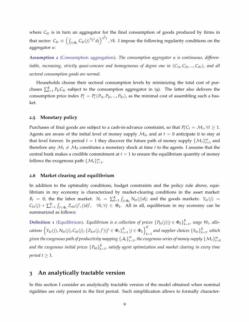
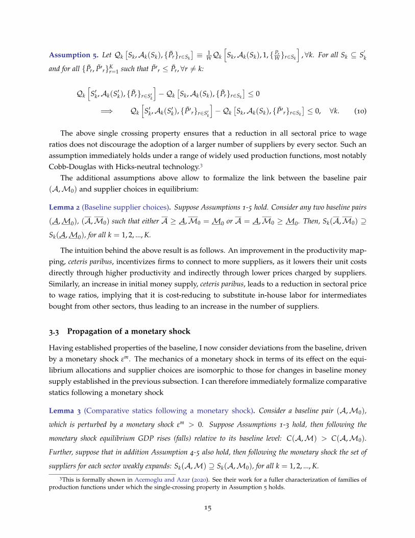
First, I use the two-sector setting consider the same small monetary expansion occurringunder different baseline productivity mappings.

Example 3 (Small monetary shocks across productivity mappings). Consider the two-sector settingwith the additional assumption on consumption aggregation: C = Cωc1

1 Cωc22 , ωck = 0.5, k = 1, 2. Panel

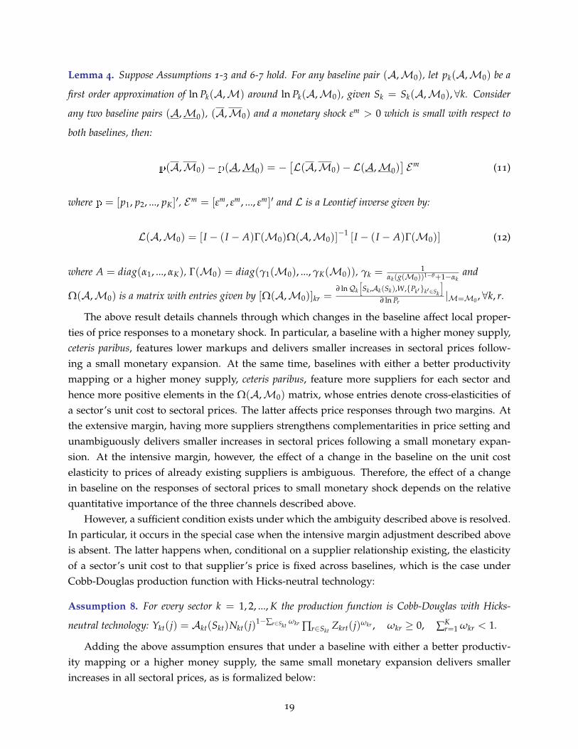
(a) of Figure 4 considers three baselines associated with different productivity mappings, as in Example1. I perturb each of the baselines with the same small monetary expansion, which, by definition, does notchange the equilibrium network. As one can see, in the low productivity baseline with the empty network,only the sticky-price Sector 2 responds to the shock; in the medium-productivity baseline the situation isunchanged, as Sector 1 does not buy inputs from Sector 2, and hence inherits no stickiness. However, inhigh-productivity state, where both sectors buy from each other, both sectors see their final consumptionrise. We can see that the magnitude of both sectoral and aggregate final consumption’s response to amonetary shock is weakly larger in baselines with higher productivity.

Similarly, I use the two-sector setting to consider the same small monetary expansion occur-ring under different levels of initial money supply.

Example 4 (Small monetary shocks across initial money supplies). Consider the two-sector settingwith the additional assumption on consumption aggregation: C = Cωc1

1 Cωc22 , ωck = 0.5, k = 1, 2. Panel

16

(b) of Figure 6 considers three baselines with different levels of initial money supply, as in Example 2.I perturb each of the baselines with the same small monetary expansion, which, by definition, does notchange the equilibrium network. One can see that in the tight money baseline only the sticky-price Sector2 responds to the shock; in the normal money baseline flexible-price Sector 1 buys from Sector 2 and inheritsstickiness, hence responding to the shock. Finally, in the loose money baseline both sectors buy from eachother and respond by even more than in the normal money state. Overall, one can see that both sectoraland aggregate consumption respond weakly stronger under baselines with higher initial money supply.

One can see that in the examples above, following a small monetary shock of the same size,consumption responds more strongly in states that feature more linkages across sectors. This isbecause whenever a sector increases the number of suppliers, its marginal cost becomes functionof a larger number of other sectoral prices, which in turn strengthens complementarities in pricesetting and the degree of money non-neutrality.

The above mechanism can be formalized by noticing that the existence of a small monetaryshock around a specific baseline implies that there is a neighborhood within which variations inmoney supply do not affect the equilibrium set of supplier choices. The latter in turn means thatsuch a neighborhood features no discontinuities created by formation or destruction of linkages,and one can appeal to local properties around the baseline. In order to establish analyticallytractable local properties, I make several further assumptions. First, a vital required additionalassumption is differentiability of the production function in labor and intermediate inputs:

Assumption 6. For every sector, the production function Fk is differentiable in(

Nkt(j), Zkrt(j)r∈Skt

).

The second additional assumption concerns the initial sectoral prices, which have so far beenassumed to be completely exogenous:

Assumption 7 (Initial sectoral prices). For every sector k = 1, 2, ..., K, the initial sectoral price is given

by Pk0 = (1 + µk)g(M0)Qk[Sk,Ak(Sk),M0, Pr(A,M0)r∈Sk ], where (A,M0) is the baseline pair,

µk = (1 + τk)θ

θ−1 and g : R+ → (0, 1) and strictly decreasing on the whole domain.

The above assumption states that for every sector the initial price is set at a fixed markup overthe baseline (steady-state) unit cost, with the markup falling in the initial money supply. In thisway, I tractably capture the idea that whenever the initial money supply is high, a monetary shockis occurring in an environment with low markups, representing the interaction of price stickinesswith past loose money supply.4 Crucially, baseline comparative statics properties established inLemmas 1 and 2 continue to hold under this additional assumption about initial prices.

Armed with the two additional assumptions, I can now begin to formalize the differences inresponses to a small monetary shock that arrives under different baselines. As a first step, thelemma below documents baseline-specific local responses of sectoral prices to a monetary shock:

4With this additional assumption on initial prices, the baseline sectoral markups are given by (1 +

µk)[αkg(M0))1−θ + (1− αk)]

11−θ , ∀k, which fall inM0.

17

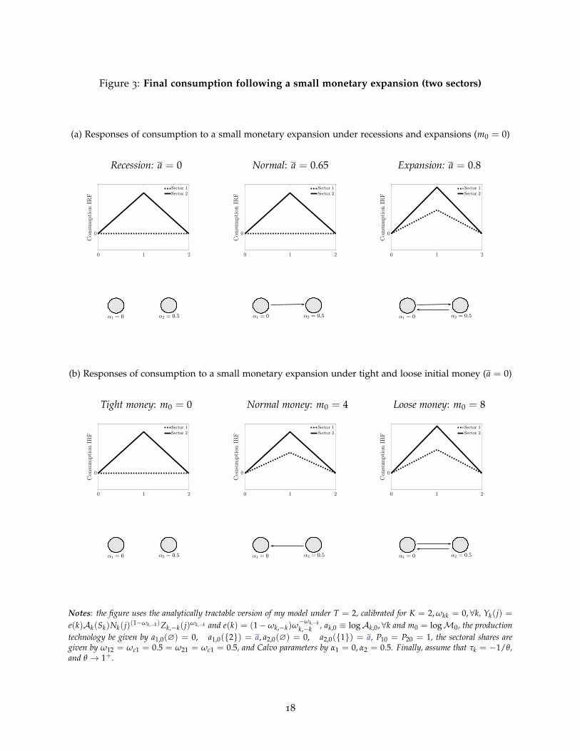
Figure 3: Final consumption following a small monetary expansion (two sectors)

(a) Responses of consumption to a small monetary expansion under recessions and expansions (m0 = 0)

Recession: a = 0 Normal: a = 0.65 Expansion: a = 0.8

(b) Responses of consumption to a small monetary expansion under tight and loose initial money (a = 0)

Tight money: m0 = 0 Normal money: m0 = 4 Loose money: m0 = 8

Notes: the figure uses the analytically tractable version of my model under T = 2, calibrated for K = 2, ωkk = 0, ∀k, Yk(j) =e(k)Ak(Sk)Nk(j)(1−ωk,−k)Zk,−k(j)ωk,−k and e(k) = (1−ωk,−k)ω

−ωk,−kk,−k , ak,0 ≡ logAk,0, ∀k and m0 = logM0, the production

technology be given by a1,0(∅) = 0, a1,0(2) = a, a2,0(∅) = 0, a2,0(1) = a, P10 = P20 = 1, the sectoral shares aregiven by ω12 = ωc1 = 0.5 = ω21 = ωc1 = 0.5, and Calvo parameters by α1 = 0, α2 = 0.5. Finally, assume that τk = −1/θ,and θ → 1+.

18

Lemma 4. Suppose Assumptions 1-3 and 6-7 hold. For any baseline pair (A,M0), let pk(A,M0) be a

first order approximation of ln Pk(A,M) around ln Pk(A,M0), given Sk = Sk(A,M0), ∀k. Consider

any two baseline pairs (A,M0), (A,M0) and a monetary shock εm > 0 which is small with respect to

both baselines, then:

p(A,M0)− p(A,M0) = −[L(A,M0)−L(A,M0)

]Em (11)

where p = [p1, p2, ..., pK]′, Em = [εm, εm, ..., εm]′ and L is a Leontief inverse given by:

L(A,M0) = [I − (I − A)Γ(M0)Ω(A,M0)]−1 [I − (I − A)Γ(M0)] (12)

where A = diag(α1, ..., αK), Γ(M0) = diag(γ1(M0), ..., γK(M0)), γk =1

αk(g(M0))1−θ+1−αkand

Ω(A,M0) is a matrix with entries given by [Ω(A,M0)]kr =∂ lnQk

[Sk ,Ak(Sk),W,Pk′k′∈Sk

]∂ ln Pr

|M=M0 , ∀k, r.

The above result details channels through which changes in the baseline affect local proper-ties of price responses to a monetary shock. In particular, a baseline with a higher money supply,ceteris paribus, features lower markups and delivers smaller increases in sectoral prices follow-ing a small monetary expansion. At the same time, baselines with either a better productivitymapping or a higher money supply, ceteris paribus, feature more suppliers for each sector andhence more positive elements in the Ω(A,M0) matrix, whose entries denote cross-elasticities ofa sector’s unit cost to sectoral prices. The latter affects price responses through two margins. Atthe extensive margin, having more suppliers strengthens complementarities in price setting andunambiguously delivers smaller increases in sectoral prices following a small monetary expan-sion. At the intensive margin, however, the effect of a change in the baseline on the unit costelasticity to prices of already existing suppliers is ambiguous. Therefore, the effect of a changein baseline on the responses of sectoral prices to small monetary shock depends on the relativequantitative importance of the three channels described above.

However, a sufficient condition exists under which the ambiguity described above is resolved.In particular, it occurs in the special case when the intensive margin adjustment described aboveis absent. The latter happens when, conditional on a supplier relationship existing, the elasticityof a sector’s unit cost to that supplier’s price is fixed across baselines, which is the case underCobb-Douglas production function with Hicks-neutral technology:

Assumption 8. For every sector k = 1, 2, ..., K the production function is Cobb-Douglas with Hicks-

neutral technology: Ykt(j) = Akt(Skt)Nkt(j)1−∑r∈Sktωkr ∏r∈Skt

Zkrt(j)ωkr , ωkr ≥ 0, ∑Kr=1 ωkr < 1.

Adding the above assumption ensures that under a baseline with either a better productiv-ity mapping or a higher money supply, the same small monetary expansion delivers smallerincreases in all sectoral prices, as is formalized below:

19

Proposition 2. Suppose Assumptions 2-5, 7-8 hold. Consider any two baseline pairs (A,M0), (A,M0)

such that either A ≥ A,M0 =M0 or A = A,M0 ≥ M0. For a monetary shock εm > 0 that is small

with respect to both baselines, it follows that pk(A,M0) ≤ pk(A,M0) for all k = 1, 2, ..., K.

Importantly, though the above proposition is formulated for a small monetary expansionεm > 0, it trivially extends to a small monetary contraction εm < 0. In particular, it would followthat under a baseline with either a better productivity mapping or a higher money supply, thesame small monetary contraction delivers smaller decreases in all sectoral prices.

I now use properties of price responses established above to study how changes in the baselineaffect consumption responses to small monetary shocks. From the cash-in-advance constraint,it follows that [ln C(A,M)− ln C(A,M0)] = εm + [ln Pc(A,M)− ln Pc(A,M0)]. It follows thatlocal properties of GDP around the baseline can be inferred from local properties of the con-sumption price index. For a monetary shock εm that is small with respect to a baseline pair(A,M0) one can write the following local approximation:

ln Pc(A,M)− ln Pc(A,M0) ≈K

∑k=1

∂ ln Pc(A,M0)

∂ ln Pk[ln Pk(A,M)− ln Pk(A,M0)] . (13)

From Proposition 2 we know local properties of (log-)deviations of sectoral prices as one variesthe baseline. However, the variation in elasticities of the consumption price index with respect tosectoral prices as one varies the baseline is ambiguous. In this sense, the local properties of ag-gregate consumption/GDP around different baselines remain on relative quantitative propertiesof movements in sectoral prices and the elasticities that are used to aggregate them.

However, a sufficient condition exists under which the ambiguity described above is resolved.In particular, it occurs in the special case when the elasticities of the consumption price indexwith respect to sectoral prices remain fixed across all baselines. The latter occurs when theconsumption aggregator takes the Cobb-Douglas form, as is detailed below:

Assumption 9. The consumption aggregator u(.) takes Cobb-Douglas form: Ct = ∏Kk=1 Cωck

kt , ωck ≥ 0,

∑Kk=1 ωck = 1.

With the additional assumption above, I can now formalize non-linear transmission of a smallmonetary shock to both sectoral and aggregate consumption, the latter being equivalent to GDPin my economy. First, whenever a small monetary expansion arrives under a baseline with abetter productivity mapping, it triggers a consumption increase of a larger magnitude:

Theorem 1 (Cycle dependence). Suppose Assumptions 3-5 and 7-9 hold. For any baseline pair (A,M0),

let ck(A,M0) ≡ ln Ck(A,M)− ln Ck(A,M0), ∀k. Consider any two baseline pairs (A,M0), (A,M0)

such that A ≥ A. For a monetary shock εm > 0 which is small with respect to both baselines it follows

that ck(A,M0) ≥ ck(A,M0) for all k = 1, 2, ..., K, and c(A,M0) ≥ c(A,M0).

20

Three points should be noted. First, although the theorem is stated for small monetaryexpansions, it trivially extends to small monetary contractions. In particular, it follows thatif a small monetary contraction arrives in a state with, ceteris paribus, higher productivity, theresulting fall in GDP is (weakly) smaller. Second, the additional assumption of Cobb-Douglasconsumption aggregation implies cycle dependence not only at the level of aggregate GDP, butalso at the level of final consumptions of individual sectors. Third, my cycle dependence resultprovides a theoretical rationale for empirical finds of procyclical magnitude of impulse responseof GDP to monetary shocks (Tenreyro and Thwaites, 2016, Alpanda et al., 2019, Jorda et al., 2019).

In a similar way, I can formalize that whenever a small monetary expansion arrives under abaseline with higher money supply, it triggers a consumption increase of a larger magnitude:

Theorem 2 (Path dependence). Suppose Assumptions 3-5 and 7-9 hold. For any baseline pair (A,M0),

let ck(A,M0) ≡ ln Ck(A,M)− ln Ck(A,M0), ∀k. Consider any two baseline pairs (A,M0), (A,M0)

such thatM0 ≥M0. For a monetary shock εm > 0 which is small with respect to both baselines it follows

that ck(A,M0) ≥ ck(A,M0) for all k = 1, 2, ..., K, and c(A,M0) ≥ c(A,M0).

As before, the theorem trivially extends to small monetary contractions: if a small monetarycontraction arrives in a state with, ceteris paribus, lower money supply, the resulting fall in GDPis (weakly) smaller. My path dependence result provides a theoretical rationale for empiricalfinds of monetary transmission to GDP being stronger under already loose monetary stance(Alpanda et al., 2019) and additional evidence that finds that GDP is more sensitive to monetaryinterventions in states of the world with already loose credit (Jorda et al., 2019).

The intuition behind both theorems is very similar. Baselines with a better productivitymapping or higher initial money supply, ceteris paribus, feature more suppliers for every sector inequilibrium. The latter strengthens complementarities in price setting, and hence deliver moremoney non-neutrality and consumption response of a larger magnitude.

3.3.2 Large monetary shocks

I now move to studying properties of large monetary shocks that are able to change the equilib-rium set of suppliers relative to the baseline. As before, I begin with building intuition using thetwo-sector setting before establishing formal results.

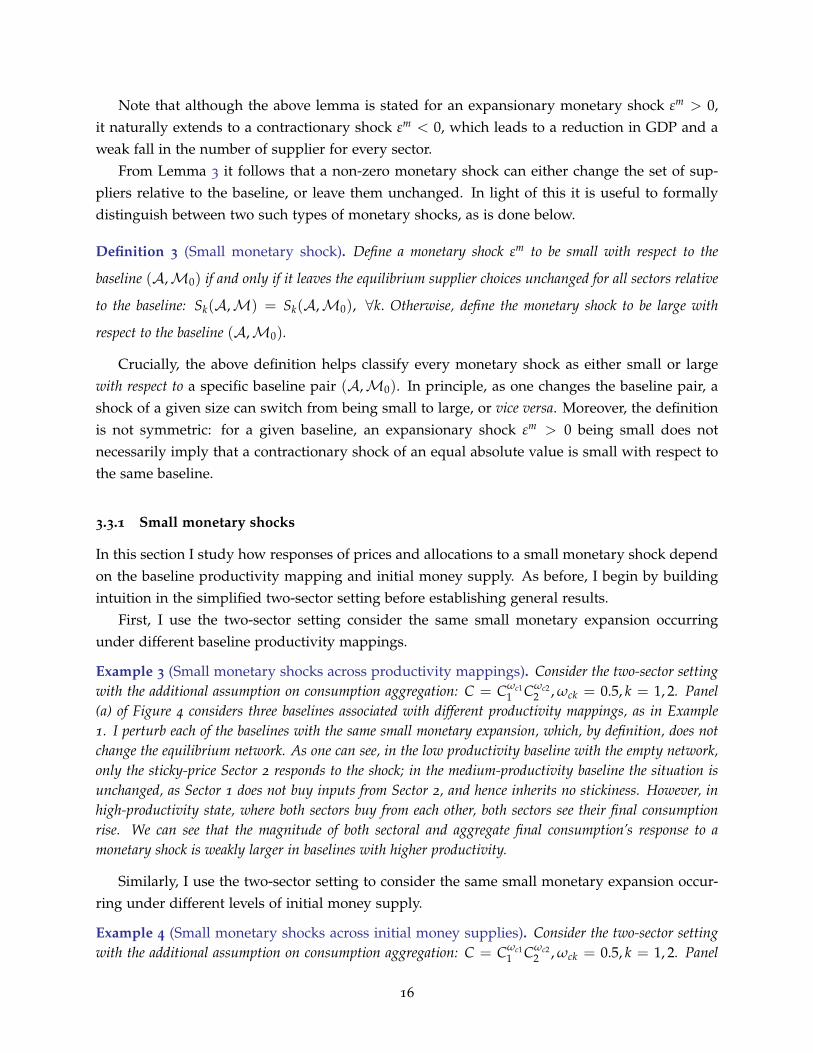
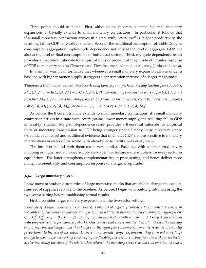
First, I consider larger monetary expansions in the two-sector setting:

Example 5 (Large monetary expansions). Panel (a) of Figure 4 considers large monetary shocks inthe context of our earlier two-sector example with an additional assumption on consumption aggregation:C = Cωc1

1 Cωc22 , ωck = 0.5, k = 1, 2. Stating with an initial state with a = m0 = 0, I subject my economy

with progressively larger monetary shocks. One can see that shocks smaller than εm = 3 keep the initiallyempty network unchanged, and the changes in the aggregate consumption impulse response are exactlyproportional to the size of the shock. However, as I consider larger expansions, they turn out to be largeenough to expand the network by encouraging the flexible-price Sector 1 to buy from the sticky-price Sector2, also increasing the slope of the relationship between the monetary shock size and consumption response.

21

Figure 4: Aggregate consumption response to large monetary shocks (two sectors)

(a) Large monetary expansions (b) Large monetary contractions

Notes: the figure uses the analytically tractable version of my model under T = 2, calibrated for K = 2, ωkk = 0, ∀k, Yk(j) =e(k)Ak(Sk)Nk(j)(1−ωk,−k)Zk,−k(j)ωk,−k and e(k) = (1−ωk,−k)ω

−ωk,−kk,−k , ak,0 ≡ logAk,0, ∀k and m0 = logM0, the production

technology be given by a1,0(∅) = 0, a1,0(2) = a, a2,0(∅) = 0, a2,0(1) = a, P10 = P20 = 1, the sectoral shares aregiven by ω12 = ωc1 = 0.5 = ω21 = ωc1 = 0.5, and Calvo parameters by α1 = 0, α2 = 0.5. Finally, assume that τk = −1/θ,and θ → 1+. Throughout exercises I set a0 = 0.

Similarly, I use the two-sector setting to study large monetary contractions:

Example 6 (Large monetary contractions). Panel (b) of Figure 4 considers large monetary contractionsin the context of the same two-sector example with an additional assumption on consumption aggregation:C = Cωc1

1 Cωc22 , ωck = 0.5, k = 1, 2 I from a baseline with a = 0 and m0 = 8. Initial reductions in money

supply leave the baseline full network unchanged and the magnitude of aggregate consumption contractionis exactly proportional to the size of the monetary shock. However, larger contractions break the network,in this case by discouraging Sector 2 from buying from Sector 1, and lower the slope of the relationshipbetween the monetary shock size and consumption response.

One can see that in the first example above, large monetary expansions deliver an increasein GDP that is larger than the one that would occur under fixed networks. In this sense, largemonetary expansions deliver more than proportional increases in GDP by expanding the set ofsuppliers for every sector. On the other hand, in the second example above, large monetarycontraction deliver reductions in GDP that are smaller in magnitude that those under exoge-nous networks. Therefore, large monetary contractions break supplier relationships and in thisway deliver less than proportional decreases in GDP, relative to the outcome under exogenousnetworks.

In order to formalize the above intuition, I introduce several new concepts. First, I letthe exact impulse response of a sectoral price to monetary shock εm be given by Pk(ε

m) ≡Pk(A,M)/Pk(A,M0), ∀k. Second, in order to facilitate comparison with a setting where sup-

22

plier choices are exogenous, I let Pek (ε

m; S) ≡ Pk(A,M, S)/Pk(A,M0, S), ∀k denote exact impulseresponses of sectoral prices to monetary shock εm in a version of my economy with an exogenousproduction network S. I am now ready to state a proposition which establishes bounds on howthe exact impulse responses of sectoral prices grow with the size of the monetary shock:

Proposition 3. Suppose Assumption 1-5 hold. For a baseline pair (A,M0), let εm > 0 be a small

monetary shock and Em > 0 be a large monetary shock. Under the large monetary shock, the equilibrium

set of supplier choices is SLk ⊃ Sk(A,M0) = S0

k , ∀k. The ratios of exact impulse responses of sectoral

prices satisfy:Pe

k (Em; SL)

Pek (ε

m; SL)≤ Pk(Em)

Pk(εm)≤ Pe(Em; S0)

Pek (ε

m; S0), (14)

for all k = 1, 2, ..., K.

Intuitively, as one moves from a small monetary expansion to a large monetary expansion,the rate at which the exact responses of sectoral prices increase is smaller than what would occurif the network stayed fixed at its baseline level. This is because the extra linkages created by thelarge monetary expansion induce additional pricing complementarities, thus reducing the rateat which prices grow. At the same time, this drag on price increases is bounded from below bywhat would occur if the network was fixed at the level delivered by the large monetary expansion.Crucially, although the above proposition is stated for monetary expansions it trivially extendsto monetary contractions by reversing the signs of inequalities. In particular, as one movesfrom a small monetary contraction to a large monetary contraction, the rate at which the exactmagnitudes of prices drops change is larger than what would occur if the network stayed fixedat its baseline level. This is because the large monetary contraction destroys some of the supplierrelationships and hence weakens pricing complementarities, allowing prices to drop faster.

Since the above proposition applies to all sectoral prices, it implies corresponding propertiesfor the aggregate consumption price index. The latter combined with the cash-in-advance in turndelivers properties of aggregate consumption, which also represents GDP in my model:

Theorem 3 (Size dependence). Suppose Assumption 1-5 hold. For a baseline pair (A,M0), let εm > 0

be a small monetary shock and Em > 0 be a large monetary shock. Under the large monetary shock, the

equilibrium set of supplier choices is SLk ⊃ Sk(A,M0) = S0

k , ∀k. The ratios of exact impulse responses of

GDP satisfy:Ce(Em; S0)

Ce(εm; S0)≤ C(Em)

C(εm)≤ Ce(Em; SL)

Ce(εm; SL). (15)

The theorem above formally establishes size-dependence in the response of GDP to monetaryshocks in my model. In particular, as one moves from a small monetary expansion to a largemonetary expansion, the rate at which the exact impulse response of GDP rises is larger thanwhat would occur if the set of suppliers was fixed at the baseline level. This is due to additional

23

pricing complementarities created by the extra linkages formed by the large monetary expansion.At the same time, the above theorem also implies that following a small monetary contractionthe rate at which the magnitude of exact impulse response of GDP changes is smaller than whatwould occur if the set of suppliers was fixed at the baseline level. This is because the largemonetary contraction destroys some of the linkages, which weakens pricing complementarities,allowing prices to drop faster and consumption to fall by less.

Crucially, I have established my size dependence results under purely time-dependence pric-ing, without appealing to menu costs or any other state-dependencies in the probability of priceadjustment. Moreover, notice that both theorems above do not require specifying the functionalform of either the production function or the consumption aggregator, and do not even imposethat the production function is differentiable.

4 A quantitative dynamic version

After establishing the key properties of my model in a simplified static version, I now quantify theeffects in a forward-looking setting calibrated to 389 sectors of the US economy. I develop a nu-merical algorithm for solving a dynamic version of my multi-sector New Keynesian model withendogenous network formation and it use to determine how changes in baseline productivityand money supply affect equilibrium supplier choices, and how the latter creates non-linearitiesin transmission of monetary shocks.

4.1 Forward-looking setting

I now quantify the effects established analytically in the previous section using a dynamicforward-looking version of my model. In particular, in this section I do not make the simplifyingassumptions needed to obtain closed-form results, and solve the model numerically. Numericalsimulations still require functional form assumptions and I therefore maintain the assumptionof Cobb-Douglas production function and Cobb-Douglas consumption aggregation. Moreover, Ineed to specify the functional form of the productivity mapping, where I augment the mappingof Acemoglu and Azar (2020) with an aggregate productivity term:

Assumption 10 (Productivity mapping). For every sector k = 1, 2, ..., K the productivity mapping

Akt(Skt) takes the following form:

Akt(Skt) = Zte(Skt)B0 ∏r∈Skt

Bkr, (16)

where Zt is aggregate productivity which follows an AR(1) process in logs: lnZt = ρz lnZt−1 + ζt, e(Skt)

is a normalization term given by e(Skt) ≡ (1− ∑r∈Sktωkr)

−(1−∑r∈Sktωkr) ∏r∈Skt

ω−ωkrkr , and B0, Bkrkr

24

are parameters.

Two points should be noted regarding the productivity mapping above. First, it delivers anequilibrium unit cost function given by Qk =

[ZtB0 ∏r∈Skt

Bkr]−1 Wt ∏r∈Skt

(PrtWt

)ωkr, ∀k, or

−zt − b0 + wt + ∑r∈Skt[ωkr(prt − wt)− bkr] in logs. The latter implies a tractable rule for whether

or not it is optimal to buy inputs from a particular supplier. Namely, sector k should only buyinputs from sector r if ωkr(prt − wt) < bkr. Second, the entire path of aggregate productivity isknown to the agents, so that they are aware of Z0 and ζt∞

t=1 at t = 0.I also need to specify the functional form of the money supply process, which I assume to

follow an AR(1) process in log-differences:

Assumption 11 (Money supply). For a given initial money supply M0, the money supply in t ≥ 1

takes the following form:

∆ lnMt = ρm∆ lnMt−1 + εmt . (17)

The agents are aware ofM0 at t = 0 and at the beginning of t = 1 discover the entire futurepath of monetary shocks εm

t ∞t=1, facing no uncertainty beyond that point.

My modified finite-horizon version of Calvo (1983) pricing, combined with the simple rulefor inclusion of suppliers described above, allows to use backward induction to solve my modelat the sector-level. Most, specifically, I am interested in solving for equilibrium for periods t < T,which feature nominal rigidities and hence real variables responding to monetary shocks. Fort ≥ T, the problem is static from firms’ pricing perspective, and money is neutral, which cantherefore be used as a terminal condition in the backward induction algorithm. Here I outlinemy method, which numerically solves for sectoral prices, supplier choices and allocations:

Algorithm 1 (New Keynesian Model with Endogenous Networks). Start from a guess for sectoral

prices, supplier choices and allocations; let X−t ,Xt and X+t be, respectively, the full set of past, present

and future prices, supplier choices and allocations at time t for any 1 ≤ t ≤ T − 1. Let P0ktK

k=1T−1t=1

be sectoral prices from the initial guess. Taking as given exogenous paths for money supply and the

productivity mapping, follow the steps below, starting from t = T − 1

(i) Taking as given sectoral supplier choices, as well as past and future variables X−t ,X+t , solve for

prices PktKk=1;

(ii) Given prices PktKk=1, update supplier choices according to the following rule: sector k should only

buy inputs from sector r if ωkr(prt −mt) < bkr, where prt ≡ ln Pkt and mt ≡ lnMt;

(iii) Taking as given X−t ,X+t , PktK

k=1 and SktKk=1, update Xt;

(iv) Repeat (i)-(iii) until convergence within the time period;

25

(v) If t > 1, decrease t by one and go back to (i). Otherwise, compare P0ktK

k=1T−1t=1 with PktK

k=1T−1t=1 ;

if they are equal, stop the algorithm; if they are not equal, set Pkt = P0kt, ∀k, 1 ≤ t ≤ T − 1, set

t = T − 1 and return to (i).

4.2 Calibration

I calibrate my model for the United States an annual frequencies. Calibration of aggregate pa-rameters is standard. I set β = 0.99 to target annualized real interest rate of 1% in steady state.The within-sector elasticity of substitution is set at θ = 6. The persistence parameters of pro-ductivity and money supply growth are set at ρa = 0.86 and ρm = 0.80, respectively. As for thethreshold beyond which there are no nominal rigidities, I choose T = 50, so that after fifty yearsall firms can adjust their prices with certainty. Finally, I normalize Z0 = 1.

As for sector-specific parameters, those are selected for the US Bureau of Economic Analysis(BEA) Detail level of disaggregation featuring K = 389 sectors. Sector-specific Calvo parametersαkK

k=1 are set as one minus the sector-specific frequency of price adjustment from Pasten et al.(2020).5 The long-run markups in my economies are given by (1 + τk)

θθ−1K

k=1 and sectoraltax rates τkK

k=1 are chosen to match the estimated sectoral markups from De Loecker et al.(2020). The observed input-output shares ωkrkr are calibrated using the 2007 BEA Input-Outputtable, whereas input-output shares for linkages not observed in the data are imputed followingAcemoglu and Azar (2020) by setting each unobserved share equal to 0.95 of the cost share oflabor of the buying sector divided by the number of potential additional suppliers for that sector.Finally, B0 and Bkrkr are estimated to ensure the steady-state equilibrium of my economyunderMt = Zt = 1, ∀t simultaneously matches observed input-output linkages and real GDPin 2007.

4.3 Simulation results

4.3.1 Baseline economies

Variations in the baseline of my economy are driven by changes in the initial money supplyM0

and changes in the sequence ζt∞t=1, which pins down the path of aggregate productivity. I

consider two sets of variations in the baseline. First, I hold M0 = 1 and ζt = 0, ∀t ≥ 2, andconsider values of ζ1 = −3%,−2%,−1%, 0, 1%, 2%, 3%. In this way, I look at baselines withboth low and high productivity paths, all of which eventually converge to the initial value ofZ0 = 1; the case of ζ1 = 0 where aggregate productivity remains fixed at the initial value is setas a benchmark against which the other baselines are compared. Second, I hold ζt = 0, ∀t ≥ 1and consider different values of M0. In particular, I assume that in the unmodelled past beforet = 0 money supply starts from M−∞ = 1 and follows the process in (17), experiencing a one-time never repeating shock εm

−∞, eventually converging to the value of M0. I consider values of5I am grateful to Michael Weber for sharing sectoral frequencies of price adjustment with me.

26

εm−∞ = −6%,−4%,−2%, 0, 2%, 4%, 6%, where the case of εm

−∞ = 0 is treated as a benchmarkagainst which all the other baselines are compared.

Panels (a) and (b) of Figure 5 consider baselines with different aggregate productivity pathsand their associated paths of average number of suppliers and average intermediates intensity,which measures the average share of total costs that goes to suppliers. Relative to the fixed-productivity baseline (ζ1 = 0), letting ζ1 = 1% is associated with a long-lived increase by around15 in the average number of suppliers per sector, which translates into an increase in averageintermediates intensity by around 0.04. Similarly, setting ζ1 = 3%, which delivers a baseline withan even better aggregate productivity, increases the average number of suppliers per sector byaround 27, or an approximately 0.06 increase in average intermediates intensity. Importantly,the results suggest that the effect of changing the baseline productivity path is not symmetric,which is a quantitative result specific to the parameters of the productivity mapping Bkrkr Ihave estimated. Specifically, a low-productivity baseline with ζ1 = −1% decreases the number ofsuppliers only by approximately 2 per sector, or a small decrease of 0.002 in average intermediatesintensity. Under an even worse productivity baseline with ζ1 = −3%, the average number ofsuppliers falls by around 8 per sector, equivalent to a 0.01 reduction in average intermediatesintensity.

As for results under baselines with different initial levels of money supply, those are reportedin Panels (c) and (d) of Figure 5. Relative the benchmark case (εm

−∞ = 0,M0 = 1), a looser moneysupply baseline under εm

−∞ = 2% features an initial rise in the average number of suppliers byaround 16, or an increase in the average intermediates intensity by around 0.045. A baselinewith an even looser initial money supply (εm

−∞ = 6%) is associated with an initial increase in theaverage number of suppliers by around 28, equivalent to a 0.06 increase in average intermediatesintensity. Just like with variations in baseline aggregate productivity, the effect of variationsin initial money supply is not symmetric. In particular, a baseline with tighter money supply(εm−∞ = −2%) has a initial drop in the average number of suppliers by 15, or a 0.005 reduction in

average intermediates intensity. An even tighter initial money supply (εm−∞ = −6%) features a

drop of 15 in average number of supplier, or a 0.012 reduction in average intermediates intensity.

4.3.2 Small monetary shocks

I now perturb each of the baselines considered in the previous subsection with the same monetaryshock, which is small in the sense that it leaves the equilibrium set of suppliers unchangedrelative to the baseline in every period. The aim is to study how variations in the baseline affectthe magnitude of monetary transmission to GDP.

Figure 6(a) shows IRFs of GDP to the same small monetary expansionary shock under base-lines with low (ζ1 = −3%) and high (ζ1 = 3%) aggregate productivity. One can see that underhigh productivity the response of GDP is persistently higher across horizons, despite the fact thatthe size of the shock is the same across the two baselines. This is because, as seen in Figure 5(a),under the high productivity baseline the average number of suppliers is higher, which strength-

27

Figure 5: Numbers of suppliers and intermediates intensities across baselines

(a) Average number of suppliers

0 2 4 6Horizon (years)

-10

0

10

20

30

Num

ber

of s

uppl

iers

+1% +2% +3% -1% -2% -3%

(b) Average intermediates intensity

0 2 4 6Horizon (years)

-0.01

0

0.01

0.03

0.05

0.07

0.09

Inte

rmed

iate

s in

tens

ity

+1% +2% +3% -1% -2% -3%

(c) Average number of suppliers

0 2 4 6Horizon (years)

-10

0

10

20

30

Num

ber

of s

uppl

iers

+2% +4% +6% -2% -4% -6%

(d) Average intermediates intensity

0 2 4 6Horizon (years)

-0.01

0

0.01

0.03

0.05

0.07

Inte

rmed

iate

s in

tens

ity

+2% +4% +6% -2% -4% -6%

Notes: Panels (a) and (b) show the average number of suppliers and average intermediates intensities across baselines whereM0 = 1 and ζt = 0, ∀t ≥ 2, and consider values of ζ1 = −3%,−2%,−1%, 1%, 2%, 3%, relative to ζ1 = 0; Panels (c) and(d) show the average number of suppliers and average intermediates intensities across baselines where ζt = 0, ∀t ≥ 1 and valuesof εm−∞ = −6%,−4%,−2%, 2%, 4%, 6%, relative to the case where εm

−∞ = 0.

28

ens complementarities in price setting and amplifies monetary non-neutrality. Moreover, Figure5(a) also shows that under the high productivity baseline the increase in the average number ofsuppliers is persistent, which is what creates persistently higher non-neutrality of money, andexplains why the gap between the two IRFs holds across horizons.

In order to further quantify such interplay between baseline productivity and monetary non-neutrality, Figure 6(b) plots peaks of IRFs of GDP to the same small monetary expansion acrossbaselines with different aggregate productivities. For the ease of interpretation, the peak underthe lowest productivity baseline (ζ1 = −3%) is normalized to one. One can see that peakresponse of GDP under the highest productivity baseline is almost one fifth larger than underthe lowest productivity baseline. However, the rate at which monetary non-neutrality varies withbaseline productivity is highly non-linear. In particular, the change in non-neutrality betweenthe highest productivity baseline (ζ1 = 3%) and the benchmark case (ζ1 = 0) is almost seventimes larger than the change between the benchmark case and the lowest productivity baseline(ζ1 = −3%). In this sense, in my quantitative model monetary policy becomes powerful inexpansions relative to normal times, but its effectiveness does not wane by nearly as much inrecessions. The latter is explained by the asymmetry in the relationship between the averagenumber of suppliers and baseline productivity, as documented in Figure 5(a).

I now repeat the above exercise for baselines that differ in their initial money supply. Figure6(c) shows IRFs of GDP to the same small monetary expansionary shock under baselines withtight (εm

−∞ = −6%) and loose (εm−∞ = 6%) initial money supply. One can see that under loose

initial money supply the response of GDP is higher across horizons. As before, this is becauseunder the loose initial money supply baseline the average number of suppliers is higher, whichstrengthens complementarities in price setting and amplifies monetary non-neutrality. Noticethat according to Figure 5(c), the change in average number of suppliers triggered by change ininitial money supply is much shorter lived that that caused by changes in baseline productivity.As a result, additional monetary non-neutrality created by high initial money supply is shorterlived and, as can be seen in Figure 6(c), IRFs of GDP under different baseline money suppliesconverge to each other faster than in Figure 6(a).

In Figure 6(d) I plot peaks of GDP responses to the same small monetary expansion acrossbaselines with different initial money supply. One can see that peak response of GDP under thebaseline with most loose money supply (εm

−∞ = 6%) is almost one tenth larger than under thebaseline with tightest money supply (εm

−∞ = −6%). As in Figure 6(b) the relationship betweenpeak GDP and changes in the baseline is highly non-linear: the drop in potency of monetarypolicy under tight initial money supply is much smaller than the rise in potency under looseinitial money. And just as before, this is explained by the asymmetry in the relationship betweenthe average number of suppliers and baseline money supply, as documented in Figure 5(c).

29

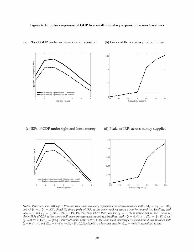
Figure 6: Impulse responses of GDP to a small monetary expansion across baselines

(a) IRFs of GDP under expansion and recession

0 1 2 3 4 5 6Horizon (years)

Agg

rega

te C

onsu

mpt

ion

(GD

P)

Small monetary expansion (+3% TFP baseline)Small monetary expansion (-3% TFP baseline)

(b) Peaks of IRFs across productivities

-3% -2% -1% 0 1% 2% 3%Productivity baseline

1

1.05

1.1

1.15

(c) IRFs of GDP under tight and loose money

0 1 2 3 4 5 6Horizon (years)

Agg

rega

te C

onsu

mpt

ion

(GD

P)

Small monetary expansion (+6% initial money supply)Small monetary expansion (-6% initial money supply)

(d) Peaks of IRFs across money supplies

-6% -4% -2% 0 2% 4% 6%Initial money supply

1

1.02

1.04

1.06

1.08

1.1

Notes: Panel (a) shows IRFs of GDP to the same small monetary expansion around two baselines, with (M0 = 1, ζ1 = −3%)and (M0 = 1, ζ1 = 3%); Panel (b) shows peaks of IRFs to the same small monetary expansion around two baselines, withM0 = 1 and ζ1 = −3%,−2%, 0,−1%, 1%, 2%, 3%, where that peak for ζ1 = −3% is normalized to one. Panel (c)shows IRFs of GDP to the same small monetary expansion around two baselines, with (ζt = 0, ∀t ≥ 1, εm

−∞ = −6%) and(ζt = 0, ∀t ≥ 1, εm

−∞ = 6%); Panel (d) shows peaks of IRFs to the same small monetary expansion around two baselines, withζt = 0, ∀t ≥ 1 and εm

−∞ = −6%,−4%,−2%, 0, 2%, 4%, 6% , where that peak for εm−∞ = −6% is normalized to one.

30

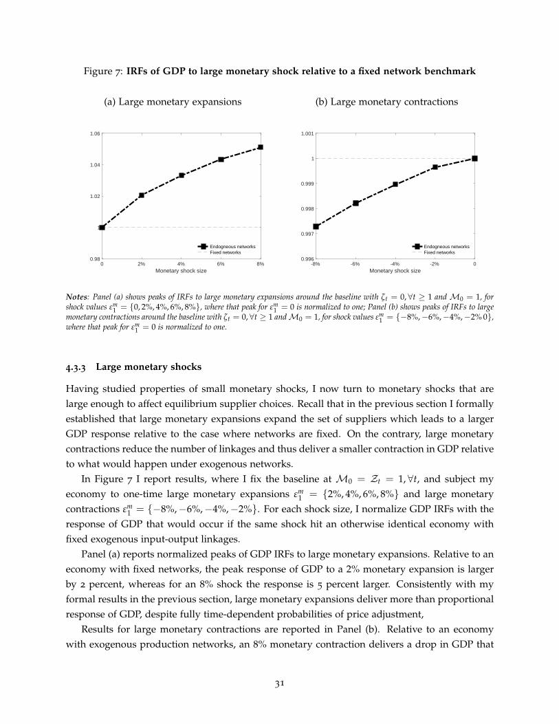
Figure 7: IRFs of GDP to large monetary shock relative to a fixed network benchmark

(a) Large monetary expansions

0 2% 4% 6% 8%Monetary shock size

0.98

1

1.02

1.04

1.06

Endogneous networksFixed networks

(b) Large monetary contractions

-8% -6% -4% -2% 0Monetary shock size

0.996

0.997

0.998

0.999

1

1.001

Endogneous networksFixed networks

Notes: Panel (a) shows peaks of IRFs to large monetary expansions around the baseline with ζt = 0, ∀t ≥ 1 and M0 = 1, forshock values εm

1 = 0, 2%, 4%, 6%, 8%, where that peak for εm1 = 0 is normalized to one; Panel (b) shows peaks of IRFs to large

monetary contractions around the baseline with ζt = 0, ∀t ≥ 1 andM0 = 1, for shock values εm1 = −8%,−6%,−4%,−2% 0,

where that peak for εm1 = 0 is normalized to one.

4.3.3 Large monetary shocks

Having studied properties of small monetary shocks, I now turn to monetary shocks that arelarge enough to affect equilibrium supplier choices. Recall that in the previous section I formallyestablished that large monetary expansions expand the set of suppliers which leads to a largerGDP response relative to the case where networks are fixed. On the contrary, large monetarycontractions reduce the number of linkages and thus deliver a smaller contraction in GDP relativeto what would happen under exogenous networks.

In Figure 7 I report results, where I fix the baseline at M0 = Zt = 1, ∀t, and subject myeconomy to one-time large monetary expansions εm

1 = 2%, 4%, 6%, 8% and large monetarycontractions εm

1 = −8%,−6%,−4%,−2%. For each shock size, I normalize GDP IRFs with theresponse of GDP that would occur if the same shock hit an otherwise identical economy withfixed exogenous input-output linkages.

Panel (a) reports normalized peaks of GDP IRFs to large monetary expansions. Relative to aneconomy with fixed networks, the peak response of GDP to a 2% monetary expansion is largerby 2 percent, whereas for an 8% shock the response is 5 percent larger. Consistently with myformal results in the previous section, large monetary expansions deliver more than proportionalresponse of GDP, despite fully time-dependent probabilities of price adjustment,

Results for large monetary contractions are reported in Panel (b). Relative to an economywith exogenous production networks, an 8% monetary contraction delivers a drop in GDP that

31

is 0.3 percent smaller at the trough, with the gap shrinking down to 0.1 percent for a 4% con-traction. Overall, the effects are consistent with formal results from the previous section, thoughtheir quantitative relevance is much smaller than under large monetary expansions. This is a con-sequence of asymmetric sensitivity of equilibrium supplier changes to changes in money supplythat was documented in Figures 5(c)-(d), where reductions in money supply do not eliminate asmany linkages as what is added under increase in money supply of the same magnitude.

5 Empirical evidence

Having established and quantified my theoretical results, I now turn to empirical assessmentof the key mechanisms. In this section I use both sectoral and firm-level input-output data toestimate network cyclicality conditional on identified technology and monetary shocks. I showthat my novel empirical results strongly support the theoretical predictions of my model.

5.1 Evidence using sector-level data

5.1.1 Data

In this subsection I use sector-level data on intermediates intensity in order to perform model-free evaluation of the predictions of my model regarding business cycle fluctuations in the shapeof the production network. In particular, I use US data on sector-level employee compensationand expenditure on intermediate inputs, published by the Bureau of Economics Analysis (BEA),to construct the share of total costs going to intermediate inputs:

δkt =Intermediate inputs costskt

Compensation of Employeeskt + Intermediate inputs costskt(18)

I construct such measure of intermediates intensity for 65 three-digit sectors of the US economyat annual frequency between 1987-2017. In the case of a Cobb-Douglas production function, suchmeasure maps directly into the model-based measure of sector-specific intermediates intensityin a particular time period, given by ∑r∈Sk,t

ωkr, ∀k.

5.1.2 Econometric strategy

Once those measures have been constructed, I use the local projection approach of Jorda (2005)in order to estimate horizon-specific impulse responses of sectoral intermediates intensity toproductivity and monetary shocks:

δk,t+H = αk,H + βHst + γHxk,t−1 + εk,t+H, (19)

32

for H = 0, 1, ..., H, where δk,t is intermediate intensity of sector k, st is an identified exogenousshock, xk,t−1 is a vector of control variables and αk,H represents horizon-specific sectoral fixedeffects. The estimated value of βH gives the horizon-specific response of intermediate inputs in-tensity to an identified exogenous shock; according to my theory, intermediates intensity should,ceteris paribus, rise following expansionary productivity and monetary shocks, and vice versa.The specification above allows to test such predictions in a transparent model-free way usinghorizon-by-horizon fixed-effects regressions.

A feature of my theory is that changes in productivity and monetary conditions can affect theequilibrium set of suppliers in a non-linear fashion. For example, in the previous section I doc-umented how improvements in productivity and money supply affect the use of intermediatesmuch more strongly than deteriorations of the same magnitude. In order to test for presence ofsuch non-linearities in the data, I consider the following augmented local projection specification:

δk,t+H = αk,H + βlinH st + β

signH st × 1st > 0+ βsize

H st × |st|+ γHxk,t−1 + εk,t+H, (20)

for H = 0, 1, ..., H, where it follows that βsignH > 0 indicates that positively-valued shocks make

the impulse response more positive, whereas βsizeH > 0 indicates that shocks which are large in

magnitude make the response more positive.In the baseline results presented in this subsection, I use identified annual productivity shocks

from Fernald (2014) and identified annual monetary shocks from Romer and Romer (2004) thathave been extended by Wieland and Yang (2016).

5.1.3 Estimation results

Figure 8 shows estimation results using linear local projections in equation (19). As one can seein Panel (a), following a positive 1% shock to aggregate productivity, the intermediates intensityresponds positively on impact, reaching peak increase of 0.004 after one year, and then graduallydeclines back to zero; such positive response is consistent with my theory. As for a monetaryexpansion, in Panel (b) shows that a surprise one-time 100bp easing leads to a slight decline inthe intermediates intensity on impact, after which it gradually increases, reaching a peak of 0.005

increase after four years; the response at longer horizons is consistent with theoretical predictionsof my model.

In Figure 9 I report results of estimation using non-linear local projections in (20). As onecan see in Panel (a), following a 1% productivity expansion, intermediates intensity rises byaround 0.01 at the peak, whereas a 3% productivity expansion increases intermediates intensityby around 0.06 at the peak. Importantly, this means that responses estimated allowing for non-linearities are not equal to linear IRFs scaled by the size of the shock, suggesting an importantrole for size effects. Moreover, Panel (e) shows that the coefficient representing size effects is sta-tistically significant at 5% level at 1-,3-,4- and 5-year horizons. Another important aspect is thatthe responses estimated allowing for non-linearities match the magnitudes of responses gener-

33

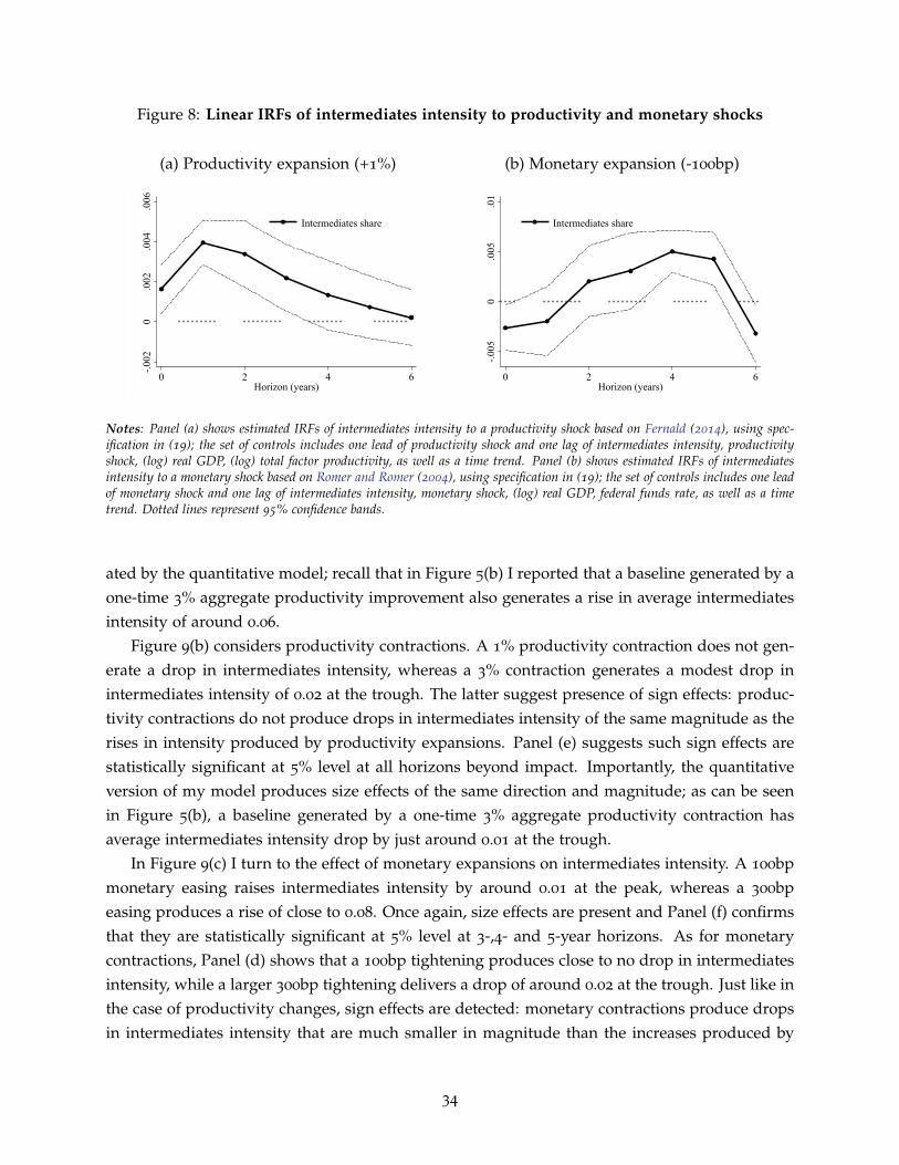
Figure 8: Linear IRFs of intermediates intensity to productivity and monetary shocks

(a) Productivity expansion (+1%)-.0

020

.002

.004

.006

0 2 4 6Horizon (years)

Intermediates share

(b) Monetary expansion (-100bp)

-.005

0.0

05.0

1

0 2 4 6Horizon (years)

Intermediates share

Notes: Panel (a) shows estimated IRFs of intermediates intensity to a productivity shock based on Fernald (2014), using spec-ification in (19); the set of controls includes one lead of productivity shock and one lag of intermediates intensity, productivityshock, (log) real GDP, (log) total factor productivity, as well as a time trend. Panel (b) shows estimated IRFs of intermediatesintensity to a monetary shock based on Romer and Romer (2004), using specification in (19); the set of controls includes one leadof monetary shock and one lag of intermediates intensity, monetary shock, (log) real GDP, federal funds rate, as well as a timetrend. Dotted lines represent 95% confidence bands.

ated by the quantitative model; recall that in Figure 5(b) I reported that a baseline generated by aone-time 3% aggregate productivity improvement also generates a rise in average intermediatesintensity of around 0.06.

Figure 9(b) considers productivity contractions. A 1% productivity contraction does not gen-erate a drop in intermediates intensity, whereas a 3% contraction generates a modest drop inintermediates intensity of 0.02 at the trough. The latter suggest presence of sign effects: produc-tivity contractions do not produce drops in intermediates intensity of the same magnitude as therises in intensity produced by productivity expansions. Panel (e) suggests such sign effects arestatistically significant at 5% level at all horizons beyond impact. Importantly, the quantitativeversion of my model produces size effects of the same direction and magnitude; as can be seenin Figure 5(b), a baseline generated by a one-time 3% aggregate productivity contraction hasaverage intermediates intensity drop by just around 0.01 at the trough.

In Figure 9(c) I turn to the effect of monetary expansions on intermediates intensity. A 100bpmonetary easing raises intermediates intensity by around 0.01 at the peak, whereas a 300bpeasing produces a rise of close to 0.08. Once again, size effects are present and Panel (f) confirmsthat they are statistically significant at 5% level at 3-,4- and 5-year horizons. As for monetarycontractions, Panel (d) shows that a 100bp tightening produces close to no drop in intermediatesintensity, while a larger 300bp tightening delivers a drop of around 0.02 at the trough. Just like inthe case of productivity changes, sign effects are detected: monetary contractions produce dropsin intermediates intensity that are much smaller in magnitude than the increases produced by

34

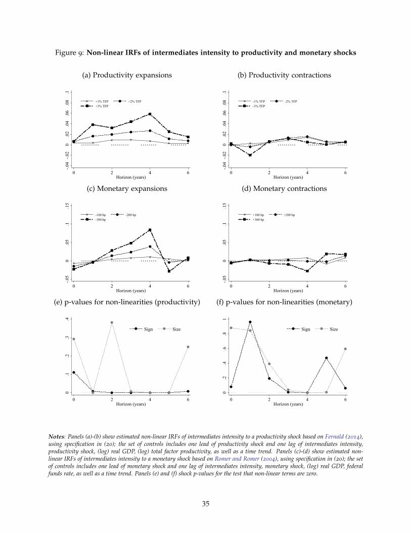
Figure 9: Non-linear IRFs of intermediates intensity to productivity and monetary shocks

(a) Productivity expansions-.0

4-.0

20

.02

.04

.06

.08

.1

0 2 4 6Horizon (years)

+1% TFP +2% TFP+3% TFP

(b) Productivity contractions

-.04

-.02

0.0

2.0

4.0

6.0

8.1

0 2 4 6Horizon (years)

-1% TFP -2% TFP-3% TFP

(c) Monetary expansions

-.05

0.0

5.1

.15

0 2 4 6Horizon (years)

-100 bp -200 bp-300 bp

(d) Monetary contractions

-.05

0.0

5.1

.15

0 2 4 6Horizon (years)

+100 bp +200 bp+300 bp

(e) p-values for non-linearities (productivity)

0.1

.2.3

.4

0 2 4 6Horizon (years)

Sign Size

(f) p-values for non-linearities (monetary)

0.2

.4.6

.81

0 2 4 6Horizon (years)

Sign Size

Notes: Panels (a)-(b) show estimated non-linear IRFs of intermediates intensity to a productivity shock based on Fernald (2014),using specification in (20); the set of controls includes one lead of productivity shock and one lag of intermediates intensity,productivity shock, (log) real GDP, (log) total factor productivity, as well as a time trend. Panels (c)-(d) show estimated non-linear IRFs of intermediates intensity to a monetary shock based on Romer and Romer (2004), using specification in (20); the setof controls includes one lead of monetary shock and one lag of intermediates intensity, monetary shock, (log) real GDP, federalfunds rate, as well as a time trend. Panels (e) and (f) shock p-values for the test that non-linear terms are zero.

35

easings of the same size. Moreover, Panel (f) suggests such sign effects are statistically significantat 3- and 4-year horizons, exactly where peaks and troughs of responses occur. Finally, recallthat in Figure 5(d) I documented presence of similar sign effects in the quantitative version of mymodel as one varies money supply.

5.1.4 Further results and robustness checks

In Appendix B I perform further econometric exercises and robustness checks, which I brieflysummarize here.

First, I re-estimate the effect of identified shocks on intermediates intensity, allowing for non-linearity, at the level of six broad sectoral groups, to determine if the observed network cyclicalitycould be driven by specific parts of the US economy. Results suggest that largest sensitivities ofintermediates intensities to changes in productivity are detected in ”Trade, transportation andwarehousing” and ”Durable manufacturing goods”, whereas very little responsiveness is foundin ”Information, Finance-Insurance-Real Estate and other services” and ”Education, healthcareand other services”. As for the effect of monetary interventions, by far the largest responseis found in ”Non-manufacturing goods”, whereas the smallest effect is found in ”Education,healthcare and other services”.

Second, I consider an alternative approach to modeling non-linearity in my local projectionssetting. In particular, I re-estimate (20), where instead of adding interactions with a sign dummyand absolute value of the shock, I add quadratic and cubic shocks, which similarly capturepossible sign and size effects. Reassuringly, results remain virtually unchanged, both in termsof magnitudes of effects, as well as when it comes to sign and size effects and their statisticalsignificance.

5.2 Evidence using firm-level data

5.2.1 Data

My model predicts that adjustments in the reliance of sectors on intermediate inputs happenon the extensive margin. However, results in the previous subsection give no guidance on thespecific margin of adjustment. In this subsection I use firm-level data on the number of suppliersof US publicly listed firms in order to perform model-free evaluation of the extensive margin ofnetwork adjustment over the business cycle. In particular, I use the dataset constructed by Atalayet al. (2011) based on US Compustat data, which contains the indegree, or simply the number ofsupplier firms in the dataset, for a large number of US publicly listed firms.

5.2.2 Econometric strategy

Using the indegree measure, I once again follow the local projection approach of Jorda (2005) inorder to estimate horizon-specific impulse responses of a firm’s number of suppliers to produc-

36

tivity and monetary shocks:

indegj,t+H = αj,H + βHst + γHxj,t−1 + ε j,t+H, (21)

for H = 0, 1, ..., H, where indegj,t is the indegree (number of suppliers) of firm j in year t, st isan identified exogenous shock, xj,t−1 is a vector of control variables and αj,H represents horizon-specific firm fixed effect. The estimated value of βH gives the horizon-specific response of thenumber of suppliers to an identified exogenous shock; according to my theory, the number ofsuppliers should, ceteris paribus, rise following expansionary productivity and monetary shocks,and vice versa. The specification above allows to test such predictions in a transparent model-freeway using horizon-by-horizon fixed-effects regressions.

As discussed earlier, my model predicts a non-linear relationship between changes in pro-ductivity and monetary conditions, and the equilibrium set of suppliers. In order to test for suchnon-linear adjustment at the extensive margin, I once again extend the previous specification toinclude additional terms:

indegj,t+H = αj,H + βlinH st + β

signH st × 1st > 0+ βsize

H st × |st|+ γHxj,t−1 + ε j,t+H, (22)

for H = 0, 1, ..., H, where it follows that βsignH > 0 indicates that positively-valued shocks make

the impulse response more positive, whereas βsizeH indicates that larger shocks make the response

more positive.In the baseline results presented in this subsection, I once again use identified annual pro-

ductivity shocks from Fernald (2014) and identified annual monetary shocks from Romer andRomer (2004) that have been extended by Wieland and Yang (2016).

5.2.3 Estimation results

Figure 10 shows estimation results using linear local projections in (21). As one can see, follow-ing a positive 1% shock to aggregate productivity, the (average) number of suppliers respondspositively on impact, reaching peak increase of around 0.20 after one year, and then graduallydeclines back to zero; such positive response is consistent with my theory. As for a monetary ex-pansion, a surprise one-time 100bp easing first leads to a slight insignificant decline, after whichin gradually increases, reaching a peak of 0.85 increase after four years; once again, the responseat longer horizons is both statistically significant and consistent with theoretical predictions.

In Figure 11 I report results obtained using non-linear local projections in (22). Panel (a) showsthat following a 1% productivity expansion, the (average) number of suppliers goes up by almost2 at the peak, whereas a 3% productivity expansion increases the number of suppliers per firm byapproximately 5. At the same time, Panel (b) suggest that productivity contractions are unableto deliver drops in the number of suppliers. The latter suggests that sign effects, documentedboth in estimation using sectoral data and in the quantitative version of my model, are similarly

37

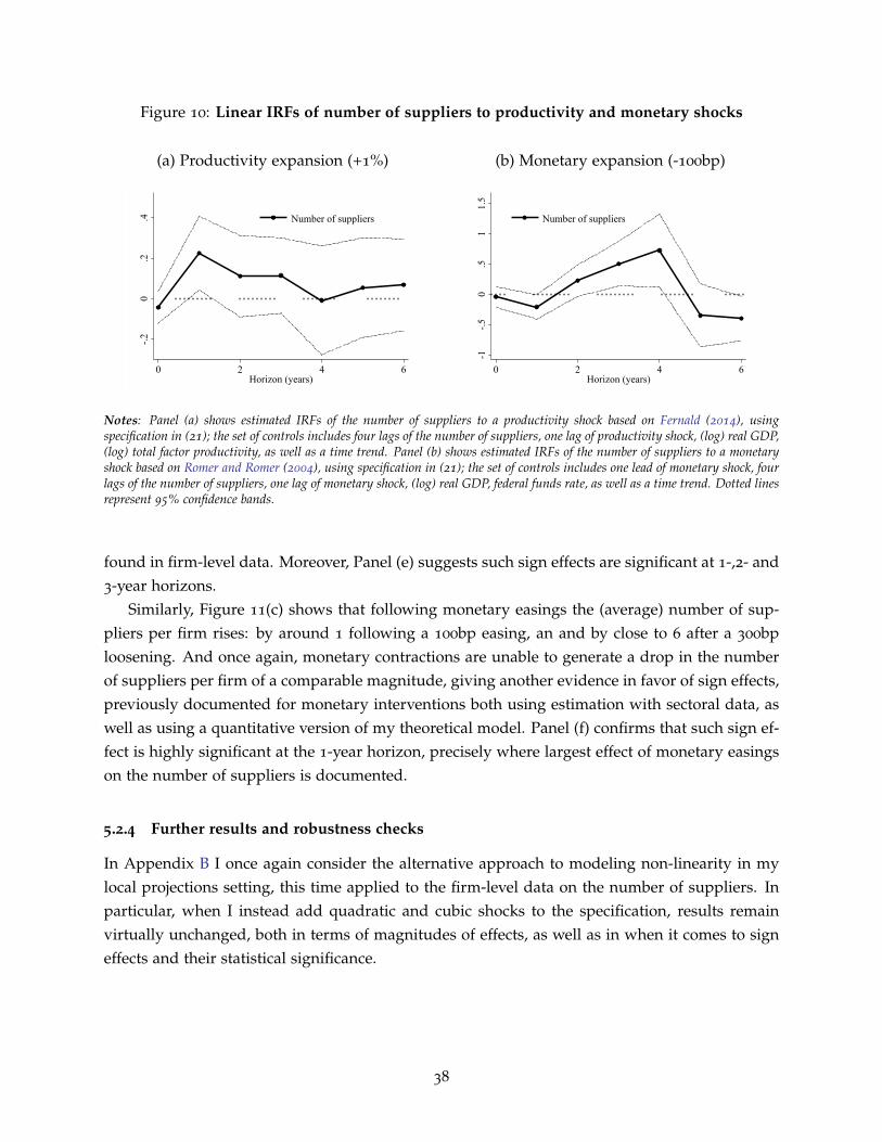
Figure 10: Linear IRFs of number of suppliers to productivity and monetary shocks

(a) Productivity expansion (+1%)-.2

0.2

.4

0 2 4 6Horizon (years)

Number of suppliers

(b) Monetary expansion (-100bp)

-1-.5

0.5

11.

5

0 2 4 6Horizon (years)

Number of suppliers

Notes: Panel (a) shows estimated IRFs of the number of suppliers to a productivity shock based on Fernald (2014), usingspecification in (21); the set of controls includes four lags of the number of suppliers, one lag of productivity shock, (log) real GDP,(log) total factor productivity, as well as a time trend. Panel (b) shows estimated IRFs of the number of suppliers to a monetaryshock based on Romer and Romer (2004), using specification in (21); the set of controls includes one lead of monetary shock, fourlags of the number of suppliers, one lag of monetary shock, (log) real GDP, federal funds rate, as well as a time trend. Dotted linesrepresent 95% confidence bands.

found in firm-level data. Moreover, Panel (e) suggests such sign effects are significant at 1-,2- and3-year horizons.

Similarly, Figure 11(c) shows that following monetary easings the (average) number of sup-pliers per firm rises: by around 1 following a 100bp easing, an and by close to 6 after a 300bploosening. And once again, monetary contractions are unable to generate a drop in the numberof suppliers per firm of a comparable magnitude, giving another evidence in favor of sign effects,previously documented for monetary interventions both using estimation with sectoral data, aswell as using a quantitative version of my theoretical model. Panel (f) confirms that such sign ef-fect is highly significant at the 1-year horizon, precisely where largest effect of monetary easingson the number of suppliers is documented.

5.2.4 Further results and robustness checks

In Appendix B I once again consider the alternative approach to modeling non-linearity in mylocal projections setting, this time applied to the firm-level data on the number of suppliers. Inparticular, when I instead add quadratic and cubic shocks to the specification, results remainvirtually unchanged, both in terms of magnitudes of effects, as well as in when it comes to signeffects and their statistical significance.

38

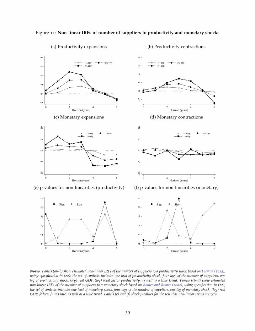
Figure 11: Non-linear IRFs of number of suppliers to productivity and monetary shocks

(a) Productivity expansions-2

02

46

8

0 2 4 6Horizon (years)

+1% TFP +2% TFP+3% TFP

(b) Productivity contractions

-20

24

68

0 2 4 6Horizon (years)

-1% TFP -2% TFP-3% TFP

(c) Monetary expansions

-10

-50

510

0 2 4 6Horizon (years)

-100 bp -200 bp-300 bp

(d) Monetary contractions

-10

-50

510

0 2 4 6Horizon (years)

+100 bp +200 bp+300 bp

(e) p-values for non-linearities (productivity)

0.2

.4.6

.81

0 2 4 6Horizon (years)

Sign Size

(f) p-values for non-linearities (monetary)

0.2

.4.6

.81

0 2 4 6Horizon (years)

Sign Size

Notes: Panels (a)-(b) show estimated non-linear IRFs of the number of suppliers to a productivity shock based on Fernald (2014),using specification in (22); the set of controls includes one lead of productivity shock, four lags of the number of suppliers, onelag of productivity shock, (log) real GDP, (log) total factor productivity, as well as a time trend. Panels (c)-(d) show estimatednon-linear IRFs of the number of suppliers to a monetary shock based on Romer and Romer (2004), using specification in (22);the set of controls includes one lead of monetary shock, four lags of the number of suppliers, one lag of monetary shock, (log) realGDP, federal funds rate, as well as a time trend. Panels (e) and (f) shock p-values for the test that non-linear terms are zero.

39

6 Conclusion

I develop a novel multi-sector New Keynesian model with roundabout production, where input-output linkages are formed endogenously through firms’ optimizing decisions. I provide novelempirical evidence on cyclical behavior of production networks and show that the model is ableto match the observed variation, conditional on either productivity or monetary shocks drivingthe cycle. In particular, in the data periods with higher productivity are associated with a largerreliance on intermediate inputs, which is also the case in the model since technological improve-ments incentivize firms to connect to more suppliers, as it lowers their unit costs directly throughhigher productivity and indirectly through lower prices charged by suppliers. At the same time,empirical evidence suggests monetary expansions lead to higher intermediates intensity, whichthe model replicates as nominal easings make prices charged by supplier firms cheaper relativeto the cost of in-house labor, incentivizing firms to connect to more suppliers.

The model delivers a novel mechanism of state-dependence in monetary transmission, whichis generated by cyclical variation in the strength of complementarities in price setting. In periodsof high productivity and loose monetary policy, firms optimally decide to connect to more sup-pliers, which strengthens pricing complementarities and amplifies monetary non-neutrality. Onthe contrary, episodes of low productivity and tight money lead to sparse networks and weakercomplementarities in price setting, which diminishes monetary non-neutrality. In this way, themodel makes monetary transmission to real variables stronger in states with (i) high productivityand (ii) previous loose monetary policy. At the same time, larger monetary expansions have a dis-proportionally bigger positive effect on GDP compared to smaller monetary expansions, whereaslarger monetary contractions have a disproportionally smaller negative effect, even if the prob-ability of price adjustment is fully time-dependent. The non-linearities in the transmission ofmonetary shocks produced by the model are consistent with those documented in model-freeeconometric studies (Tenreyro and Thwaites, 2016; Jorda et al., 2019; Alpanda et al., 2019; Ascariand Haber, 2021).

My analysis offers multiple avenues for further research. First, optimal choice of supplierscan also be studied in an open economy setting, where firms minimize their production costs bydeciding whether to purchase intermediate inputs from domestic producers or instead importthem from abroad. Such a mechanism would pin down the optimal degree of participation inglobal value chains, with immediate implications for both monetary and trade policies. Sec-ond, my analysis has focused on positive aspects of monetary transmission under endogenousproduction networks, and future work can study optimal conduct of monetary policy in such asetting. Third, a deeper quantitative assessment of the non-linearities generated by endogenousnetwork formation requires enriching the setting with medium-scale features, such as capitalaccumulation, habits-in-consumption and trend inflation to name a few.

40

References

Acemoglu, D. and P. D. Azar (2020). Endogenous production networks. Econometrica 88(1), 33–82.

Alpanda, S., E. Granziera, S. Zubairy, et al. (2019). State dependence of monetary policy acrossbusiness, credit and interest rate cycles.

Alvarez, F., F. Lippi, and J. Passadore (2017). Are state-and time-dependent models really differ-ent? NBER Macroeconomics Annual 31(1), 379–457.

Ascari, G. and T. Haber (2021, 06). Non-Linearities, State-Dependent Prices and the TransmissionMechanism of Monetary Policy. The Economic Journal. ueab049.

Atalay, E., A. Hortacsu, J. Roberts, and C. Syverson (2011). Network structure of production.Proceedings of the National Academy of Sciences 108(13), 5199–5202.

Berger, D., K. Milbradt, F. Tourre, and J. Vavra (2021, September). Mortgage prepayment andpath-dependent effects of monetary policy. American Economic Review 111(9), 2829–78.

Bernstein, J. (2021). A model of state-dependent monetary policy. Journal of Monetary Eco-nomics 117, 904–917.

Calvo, G. A. (1983). Staggered prices in a utility-maximizing framework. Journal of MonetaryEconomics 12(3), 383–398.

Carvalho, C., J. W. Lee, and W. Y. Park (2021, January). Sectoral price facts in a sticky-pricemodel. American Economic Journal: Macroeconomics 13(1), 216–56.

Carvalho, V. M. and N. Voigtlander (2015). Input diffusion and the evolution of productionnetworks.

De Loecker, J., J. Eeckhout, and G. Unger (2020). The rise of market power and the macroeco-nomic implications. The Quarterly Journal of Economics 135(2), 561–644.

Eichenbaum, M., S. Rebelo, and A. Wong (2018). State dependent effects of monetary policy: Therefinancing channel. Technical report, National Bureau of Economic Research.

Fernald, J. (2014). A quarterly, utilization-adjusted series on total factor productivity. FederalReserve Bank of San Francisco.

Ghassibe, M. (2021). Monetary policy and production networks: an empirical investigation.Journal of Monetary Economics 119, 21–39.

Hansen, G. D. (1985). Indivisible labor and the business cycle. Journal of Monetary Economics 16(3),309–327.

41

Jorda, O. (2005). Estimation and inference of impulse responses by local projections. AmericanEconomic Review 95(1), 161–182.

Jorda, O., M. Schularick, and A. M. Taylor (2019). The effects of quasi-random monetary experi-ments. Journal of Monetary Economics.

La’O, J. and A. Tahbaz-Salehi (2020, July). Optimal monetary policy in production networks.Working Paper 27464, National Bureau of Economic Research.

McKay, A. and J. F. Wieland (2019). Lumpy durable consumption demand and the limited am-munition of monetary policy. Technical report, National Bureau of Economic Research.

Milgrom, P. and C. Shannon (1994). Monotone comparative statics. Econometrica 62(1), 157–180.

Nakamura, E. and J. Steinsson (2010). Monetary non-neutrality in a multisector menu cost model.The Quarterly Journal of Economics 125(3), 961–1013.

Oberfield, E. (2018). A theory of input–output architecture. Econometrica 86(2), 559–589.

Pasten, E., R. Schoenle, and M. Weber (2020). The propagation of monetary policy shocks in aheterogeneous production economy. Journal of Monetary Economics 116, 1–22.

Romer, C. D. and D. H. Romer (2004). A new measure of monetary shocks: Derivation andimplications. American Economic Review 94(4), 1055–1084.

Rubbo, E. (2020). Networks, phillips curves, and monetary policy.

Santoro, E., I. Petrella, D. Pfajfar, and E. Gaffeo (2014). Loss aversion and the asymmetric trans-mission of monetary policy. Journal of Monetary Economics 68, 19–36.

Smets, F., J. Tielens, and J. Van Hove (2019). Pipeline pressures and sectoral inflation dynamics.NBB Working Paper Series 2019.

Taschereau-Dumouchel, M. (2019). Cascades and fluctuations in an economy with an endogenousproduction network. Available at SSRN 3115854.

Tenreyro, S. and G. Thwaites (2016). Pushing on a string: Us monetary policy is less powerful inrecessions. American Economic Journal: Macroeconomics 8(4), 43–74.

Wieland, J. F. and M.-J. Yang (2016). Financial dampening. Technical report, National Bureau ofEconomic Research.

Appendix

Endogenous production networks and non-linear monetary transmission

(Mishel Ghassibe, University of Oxford)

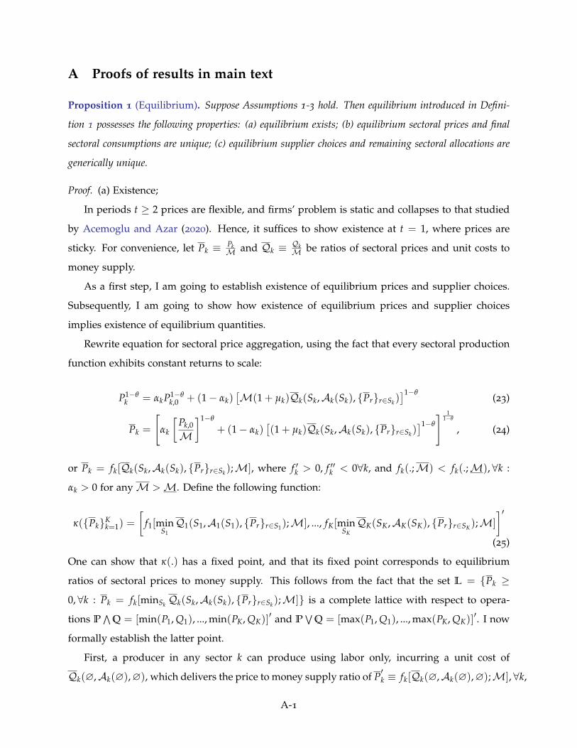
A Proofs of results in main text

Proposition 1 (Equilibrium). Suppose Assumptions 1-3 hold. Then equilibrium introduced in Defini-

tion 1 possesses the following properties: (a) equilibrium exists; (b) equilibrium sectoral prices and final

sectoral consumptions are unique; (c) equilibrium supplier choices and remaining sectoral allocations are

generically unique.

Proof. (a) Existence;

In periods t ≥ 2 prices are flexible, and firms’ problem is static and collapses to that studied

by Acemoglu and Azar (2020). Hence, it suffices to show existence at t = 1, where prices are

sticky. For convenience, let Pk ≡ PkM and Qk ≡ Qk

M be ratios of sectoral prices and unit costs to

money supply.

As a first step, I am going to establish existence of equilibrium prices and supplier choices.

Subsequently, I am going to show how existence of equilibrium prices and supplier choices

implies existence of equilibrium quantities.

Rewrite equation for sectoral price aggregation, using the fact that every sectoral production

function exhibits constant returns to scale:

P1−θk = αkP1−θ

k,0 + (1− αk)[M(1 + µk)Qk(Sk,Ak(Sk), Prr∈Sk)

]1−θ(23)

Pk =

[αk

[Pk,0

M

]1−θ

+ (1− αk)[(1 + µk)Qk(Sk,Ak(Sk), Prr∈Sk)

]1−θ

] 11−θ

, (24)

or Pk = fk[Qk(Sk,Ak(Sk), Prr∈Sk);M], where f ′k > 0, f ′′k < 0∀k, and fk(.;M) < fk(.;M), ∀k :

αk > 0 for anyM >M. Define the following function:

κ(PkKk=1) =

[f1[min

S1Q1(S1,A1(S1), Prr∈S1);M], ..., fK[min

SKQK(SK,AK(SK), Prr∈SK);M]

]′(25)

One can show that κ(.) has a fixed point, and that its fixed point corresponds to equilibrium

ratios of sectoral prices to money supply. This follows from the fact that the set L = Pk ≥

0, ∀k : Pk = fk[minSk Qk(Sk,Ak(Sk), Prr∈Sk);M] is a complete lattice with respect to opera-

tions P∧

Q = [min(P1, Q1), ..., min(PK, QK)]′ and P

∨Q = [max(P1, Q1), ..., max(PK, QK)]

′. I now

formally establish the latter point.

First, a producer in any sector k can produce using labor only, incurring a unit cost of

Qk(∅,Ak(∅),∅), which delivers the price to money supply ratio of P′k ≡ fk[Qk(∅,Ak(∅),∅);M], ∀k,

A-1

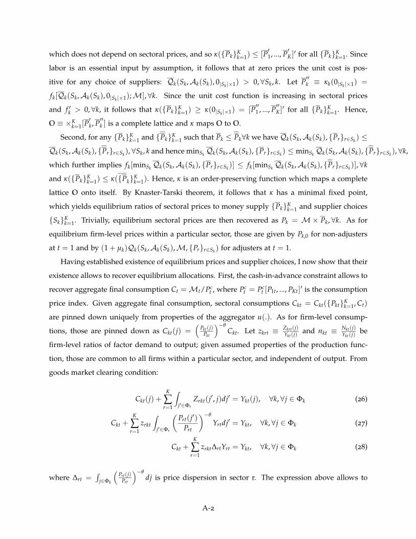
which does not depend on sectoral prices, and so κ(PkKk=1) ≤ [P′1, ..., P′K]′ for all PkK

k=1. Since

labor is an essential input by assumption, it follows that at zero prices the unit cost is pos-

itive for any choice of suppliers: Qk(Sk,Ak(Sk), 0|Sk |×1) > 0, ∀Sk, k. Let P′′k ≡ κk(0|Sk |×1) =

fk[Qk(Sk,Ak(Sk), 0|Sk |×1);M], ∀k. Since the unit cost function is increasing in sectoral prices

and f ′k > 0, ∀k, it follows that κ(PkKk=1) ≥ κ(0|Sk |×1) = [P′′1 , ..., P′′K]′ for all PkK

k=1. Hence,

O ≡ ×Kk=1[P

′k, P′′k ] is a complete lattice and κ maps O to O.

Second, for any PkKk=1 and PkK

k=1 such that Pk ≤ Pk∀k we have Qk(Sk,Ak(Sk), Prr∈Sk) ≤

Qk(Sk,Ak(Sk), Prr∈Sk), ∀Sk, k and hence minSk Qk(Sk,Ak(Sk), Prr∈Sk) ≤ minSk Qk(Sk,Ak(Sk), Prr∈Sk), ∀k,

which further implies fk[minSk Qk(Sk,Ak(Sk), Prr∈Sk)] ≤ fk[minSk Qk(Sk,Ak(Sk), Prr∈Sk)], ∀k

and κ(PkKk=1) ≤ κ(PkK

k=1). Hence, κ is an order-preserving function which maps a complete

lattice O onto itself. By Knaster-Tarski theorem, it follows that κ has a minimal fixed point,

which yields equilibrium ratios of sectoral prices to money supply PkKk=1 and supplier choices

SkKk=1. Trivially, equilibrium sectoral prices are then recovered as Pk = M× Pk, ∀k. As for

equilibrium firm-level prices within a particular sector, those are given by Pk,0 for non-adjusters

at t = 1 and by (1 + µk)Qk(Sk,Ak(Sk),M, Prr∈Sk) for adjusters at t = 1.

Having established existence of equilibrium prices and supplier choices, I now show that their

existence allows to recover equilibrium allocations. First, the cash-in-advance constraint allows to

recover aggregate final consumption Ct =Mt/Pct , where Pc

t = Pct [P1t, ..., PKt]

′ is the consumption

price index. Given aggregate final consumption, sectoral consumptions Ckt = Ckt(PktKk=1, Ct)

are pinned down uniquely from properties of the aggregator u(.). As for firm-level consump-

tions, those are pinned down as Ckt(j) =(

Pkt(j)Pkt

)−θCkt. Let zkrt ≡ Zkrt(j)

Ykt(j) and nkt ≡ Nkt(j)Ykt(j) be

firm-level ratios of factor demand to output; given assumed properties of the production func-

tion, those are common to all firms within a particular sector, and independent of output. From

goods market clearing condition:

Ckt(j) +K

∑r=1

∫j′∈Φr

Zrkt(j′, j)dj′ = Ykt(j), ∀k, ∀j ∈ Φk (26)

Ckt +K

∑r=1

zrkt

∫j′∈Φr

(Prt(j′)

Prt

)−θ

Yrtdj′ = Ykt, ∀k, ∀j ∈ Φk (27)

Ckt +K

∑r=1

zrkt∆rtYrt = Ykt, ∀k, ∀j ∈ Φk (28)

where ∆rt =∫

j∈Φk

(Prt(j)

Prt

)−θdj is price dispersion in sector r. The expression above allows to

A-2

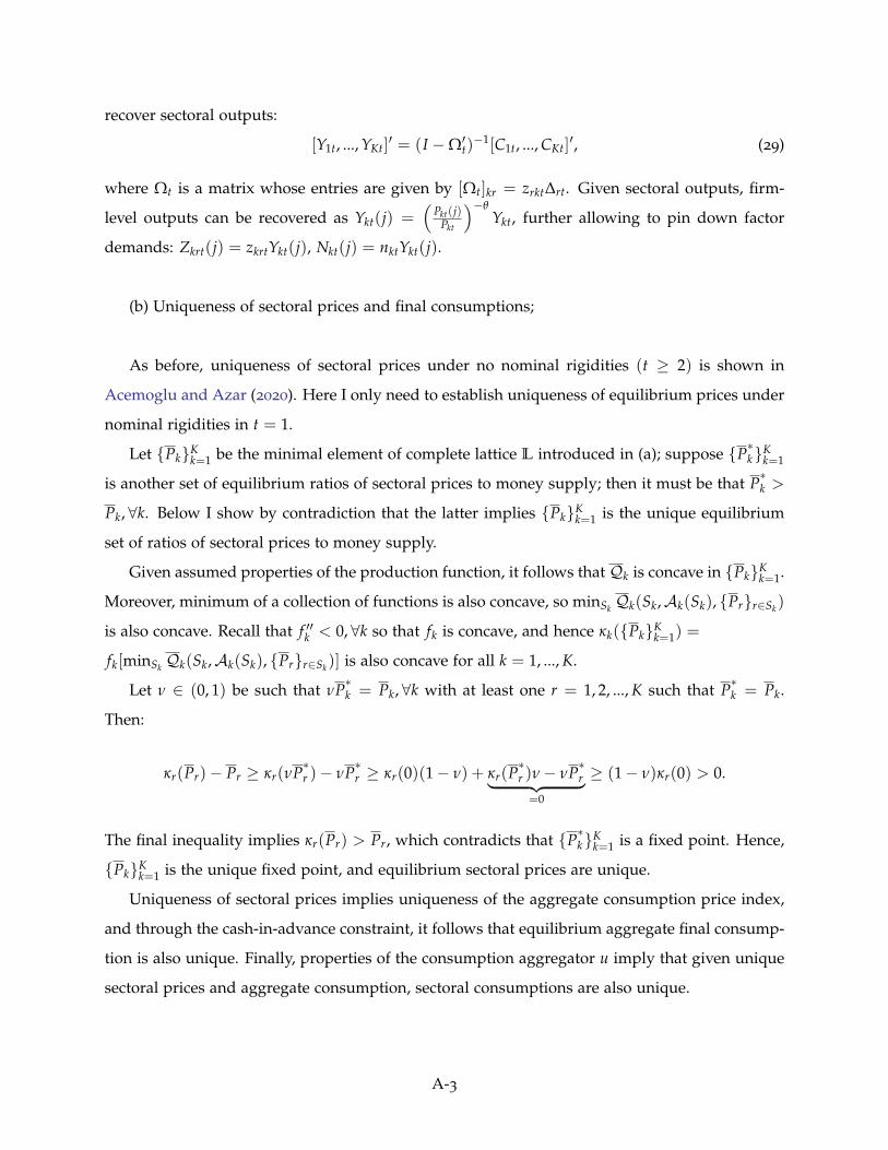
recover sectoral outputs:

[Y1t, ..., YKt]′ = (I −Ω′t)

−1[C1t, ..., CKt]′, (29)

where Ωt is a matrix whose entries are given by [Ωt]kr = zrkt∆rt. Given sectoral outputs, firm-

level outputs can be recovered as Ykt(j) =(

Pkt(j)Pkt

)−θYkt, further allowing to pin down factor

demands: Zkrt(j) = zkrtYkt(j), Nkt(j) = nktYkt(j).

(b) Uniqueness of sectoral prices and final consumptions;

As before, uniqueness of sectoral prices under no nominal rigidities (t ≥ 2) is shown in

Acemoglu and Azar (2020). Here I only need to establish uniqueness of equilibrium prices under

nominal rigidities in t = 1.

Let PkKk=1 be the minimal element of complete lattice L introduced in (a); suppose P∗kK

k=1

is another set of equilibrium ratios of sectoral prices to money supply; then it must be that P∗k >

Pk, ∀k. Below I show by contradiction that the latter implies PkKk=1 is the unique equilibrium

set of ratios of sectoral prices to money supply.

Given assumed properties of the production function, it follows that Qk is concave in PkKk=1.

Moreover, minimum of a collection of functions is also concave, so minSk Qk(Sk,Ak(Sk), Prr∈Sk)

is also concave. Recall that f ′′k < 0, ∀k so that fk is concave, and hence κk(PkKk=1) =

fk[minSk Qk(Sk,Ak(Sk), Prr∈Sk)] is also concave for all k = 1, ..., K.

Let ν ∈ (0, 1) be such that νP∗k = Pk, ∀k with at least one r = 1, 2, ..., K such that P∗k = Pk.

Then:

κr(Pr)− Pr ≥ κr(νP∗r )− νP∗r ≥ κr(0)(1− ν) + κr(P∗r )ν− νP∗r︸ ︷︷ ︸=0

≥ (1− ν)κr(0) > 0.

The final inequality implies κr(Pr) > Pr, which contradicts that P∗kKk=1 is a fixed point. Hence,

PkKk=1 is the unique fixed point, and equilibrium sectoral prices are unique.

Uniqueness of sectoral prices implies uniqueness of the aggregate consumption price index,

and through the cash-in-advance constraint, it follows that equilibrium aggregate final consump-

tion is also unique. Finally, properties of the consumption aggregator u imply that given unique

sectoral prices and aggregate consumption, sectoral consumptions are also unique.

A-3

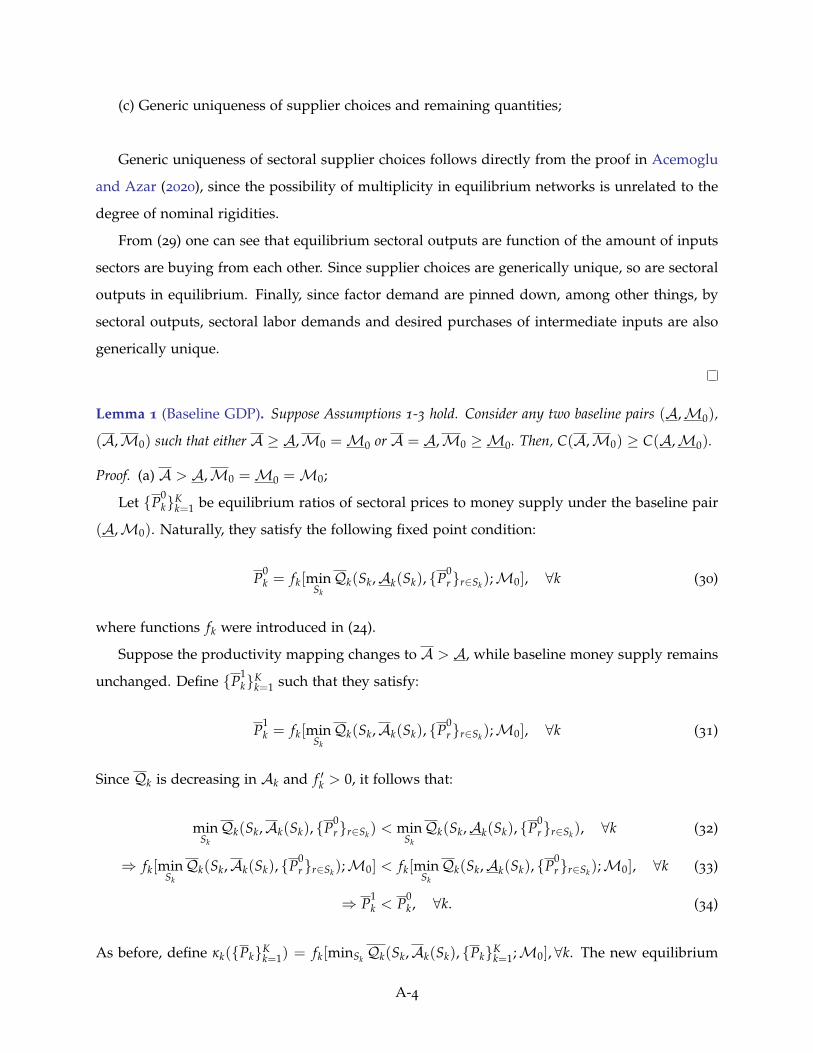
(c) Generic uniqueness of supplier choices and remaining quantities;

Generic uniqueness of sectoral supplier choices follows directly from the proof in Acemoglu

and Azar (2020), since the possibility of multiplicity in equilibrium networks is unrelated to the

degree of nominal rigidities.

From (29) one can see that equilibrium sectoral outputs are function of the amount of inputs

sectors are buying from each other. Since supplier choices are generically unique, so are sectoral

outputs in equilibrium. Finally, since factor demand are pinned down, among other things, by

sectoral outputs, sectoral labor demands and desired purchases of intermediate inputs are also

generically unique.

Lemma 1 (Baseline GDP). Suppose Assumptions 1-3 hold. Consider any two baseline pairs (A,M0),

(A,M0) such that either A ≥ A,M0 =M0 or A = A,M0 ≥M0. Then, C(A,M0) ≥ C(A,M0).

Proof. (a) A > A,M0 =M0 =M0;

Let P0kK

k=1 be equilibrium ratios of sectoral prices to money supply under the baseline pair

(A,M0). Naturally, they satisfy the following fixed point condition:

P0k = fk[min

SkQk(Sk,Ak(Sk), P

0rr∈Sk);M0], ∀k (30)

where functions fk were introduced in (24).

Suppose the productivity mapping changes to A > A, while baseline money supply remains

unchanged. Define P1kK

k=1 such that they satisfy:

P1k = fk[min

SkQk(Sk,Ak(Sk), P

0rr∈Sk);M0], ∀k (31)

Since Qk is decreasing in Ak and f ′k > 0, it follows that:

minSkQk(Sk,Ak(Sk), P

0rr∈Sk) < min

SkQk(Sk,Ak(Sk), P

0rr∈Sk), ∀k (32)

⇒ fk[minSkQk(Sk,Ak(Sk), P

0rr∈Sk);M0] < fk[min

SkQk(Sk,Ak(Sk), P

0rr∈Sk);M0], ∀k (33)

⇒ P1k < P0

k , ∀k. (34)

As before, define κk(PkKk=1) = fk[minSk Qk(Sk,Ak(Sk), PkK

k=1;M0], ∀k. The new equilibrium

A-4

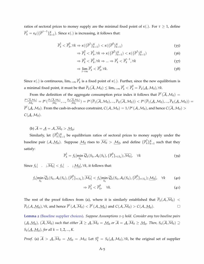
ratios of sectoral prices to money supply are the minimal fixed point of κ(.). For τ ≥ 1, define

Pτk = κk(P

τ−1Kk=1). Since κ(.) is increasing, it follows that:

P1k < P0

k , ∀k⇒ κ(P1Kk=1) < κ(P0K

k=1) (35)

⇒ P2k < P1

k , ∀k⇒ κ(P2Kk=1) < κ(P1K

k=1) (36)

⇒ P3k < P2

k , ∀k⇒ ...⇒ Ptk < Pt−1

k , ∀k (37)

⇒ limt→∞

Ptk < P0

k , ∀k. (38)

Since κ(.) is continuous, limt→∞ Ptk is a fixed point of κ(.). Further, since the new equilibrium is

a minimal fixed point, it must be that Pk(A,M0) ≤ limt→∞ Ptk < P0

k = Pk(A,M0), ∀k.

From the definition of the aggregate consumption price index it follows that Pc(A,M0) =

Pc(A,M0)M0

= Pc( P1(A,M0)M0

, ..., PK(A,M0)M0

) = Pc(P1(A,M0), ..., PK(A,M0)) < Pc(P1(A,M0), ..., PK(A,M0)) =

Pc(A,M0). From the cash-in-advance constraint, C(A,M0) = 1/Pc(A,M0), and hence C(A,M0) >

C(A,M0).

(b) A = A = A,M0 >M0;

Similarly, let P0kK

k=1 be equilibrium ratios of sectoral prices to money supply under the

baseline pair (A,M0). Suppose M0 rises to M0 > M0, and define P1kK

k=1 such that they

satisfy:

P1k = fk[min

SkQk(Sk,Ak(Sk), P

0rr∈Sk);M0], ∀k (39)

Since fk[ . ;M0] < fk[ . ;M0], ∀k, it follows that:

fk[minSkQk(Sk,Ak(Sk), P

0rr∈Sk);M0] < fk[min

SkQk(Sk,Ak(Sk), P

0rr∈Sk);M0], ∀k (40)

⇒ P1k < P0

k , ∀k. (41)

The rest of the proof follows from (a), where it is similarly established that Pk(A,M0) <

Pk(A,M0), ∀k, and hence Pc(A,M0) < Pc

(A,M0) and C(A,M0) > C(A,M0).

Lemma 2 (Baseline supplier choices). Suppose Assumptions 1-5 hold. Consider any two baseline pairs

(A,M0), (A,M0) such that either A ≥ A,M0 =M0 or A = A,M0 ≥ M0. Then, Sk(A,M0) ⊇

Sk(A,M0), for all k = 1, 2, ..., K.

Proof. (a) A > A,M0 = M0 = M0; Let S0k = Sk(A,M0), ∀k, be the original set of supplier

A-5

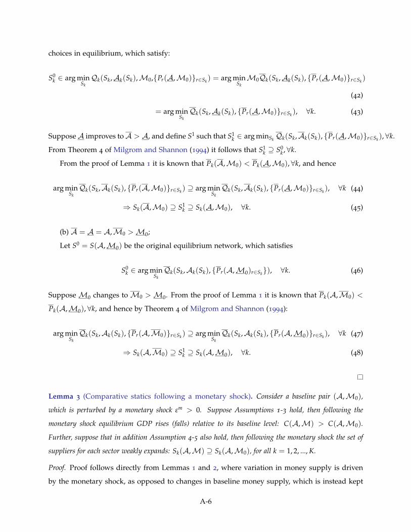
choices in equilibrium, which satisfy:

S0k ∈ arg min

SkQk(Sk,Ak(Sk),M0,Pr(A,M0)r∈Sk) = arg min

SkM0Qk(Sk,Ak(Sk), Pr(A,M0)r∈Sk)

(42)

= arg minSkQk(Sk,Ak(Sk), Pr(A,M0)r∈Sk), ∀k. (43)

SupposeA improves toA > A, and define S1 such that S1k ∈ arg minSk Qk(Sk,Ak(Sk), Pr(A,M0)r∈Sk), ∀k.

From Theorem 4 of Milgrom and Shannon (1994) it follows that S1k ⊇ S0

k , ∀k.

From the proof of Lemma 1 it is known that Pk(A,M0) < Pk(A,M0), ∀k, and hence

arg minSkQk(Sk,Ak(Sk), Pr(A,M0)r∈Sk) ⊇ arg min

SkQk(Sk,Ak(Sk), Pr(A,M0)r∈Sk), ∀k (44)

⇒ Sk(A,M0) ⊇ S1k ⊇ Sk(A,M0), ∀k. (45)

(b) A = A = A,M0 >M0;

Let S0 = S(A,M0) be the original equilibrium network, which satisfies

S0k ∈ arg min

SkQk(Sk,Ak(Sk), Pr(A,M0)r∈Sk), ∀k. (46)

Suppose M0 changes to M0 >M0. From the proof of Lemma 1 it is known that Pk(A,M0) <

Pk(A,M0), ∀k, and hence by Theorem 4 of Milgrom and Shannon (1994):

arg minSkQk(Sk,Ak(Sk), Pr(A,M0)r∈Sk) ⊇ arg min

SkQk(Sk,Ak(Sk), Pr(A,M0)r∈Sk), ∀k (47)

⇒ Sk(A,M0) ⊇ S1k ⊇ Sk(A,M0), ∀k. (48)

Lemma 3 (Comparative statics following a monetary shock). Consider a baseline pair (A,M0),

which is perturbed by a monetary shock εm > 0. Suppose Assumptions 1-3 hold, then following the

monetary shock equilibrium GDP rises (falls) relative to its baseline level: C(A,M) > C(A,M0).

Further, suppose that in addition Assumption 4-5 also hold, then following the monetary shock the set of

suppliers for each sector weakly expands: Sk(A,M) ⊇ Sk(A,M0), for all k = 1, 2, ..., K.

Proof. Proof follows directly from Lemmas 1 and 2, where variation in money supply is driven

by the monetary shock, as opposed to changes in baseline money supply, which is instead kept

A-6

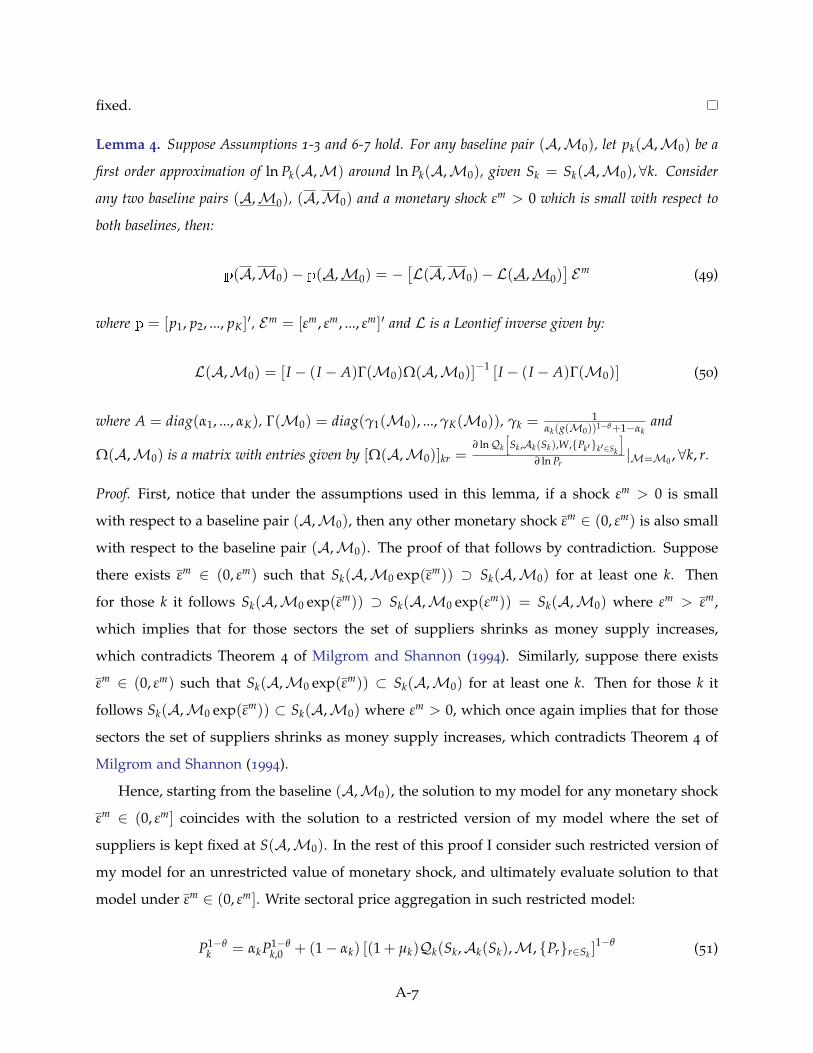
fixed.

Lemma 4. Suppose Assumptions 1-3 and 6-7 hold. For any baseline pair (A,M0), let pk(A,M0) be a

first order approximation of ln Pk(A,M) around ln Pk(A,M0), given Sk = Sk(A,M0), ∀k. Consider

any two baseline pairs (A,M0), (A,M0) and a monetary shock εm > 0 which is small with respect to

both baselines, then:

p(A,M0)− p(A,M0) = −[L(A,M0)−L(A,M0)

]Em (49)

where p = [p1, p2, ..., pK]′, Em = [εm, εm, ..., εm]′ and L is a Leontief inverse given by:

L(A,M0) = [I − (I − A)Γ(M0)Ω(A,M0)]−1 [I − (I − A)Γ(M0)] (50)

where A = diag(α1, ..., αK), Γ(M0) = diag(γ1(M0), ..., γK(M0)), γk =1

αk(g(M0))1−θ+1−αkand

Ω(A,M0) is a matrix with entries given by [Ω(A,M0)]kr =∂ lnQk

[Sk ,Ak(Sk),W,Pk′k′∈Sk

]∂ ln Pr

|M=M0 , ∀k, r.

Proof. First, notice that under the assumptions used in this lemma, if a shock εm > 0 is small

with respect to a baseline pair (A,M0), then any other monetary shock εm ∈ (0, εm) is also small

with respect to the baseline pair (A,M0). The proof of that follows by contradiction. Suppose

there exists εm ∈ (0, εm) such that Sk(A,M0 exp(εm)) ⊃ Sk(A,M0) for at least one k. Then

for those k it follows Sk(A,M0 exp(εm)) ⊃ Sk(A,M0 exp(εm)) = Sk(A,M0) where εm > εm,

which implies that for those sectors the set of suppliers shrinks as money supply increases,

which contradicts Theorem 4 of Milgrom and Shannon (1994). Similarly, suppose there exists

εm ∈ (0, εm) such that Sk(A,M0 exp(εm)) ⊂ Sk(A,M0) for at least one k. Then for those k it

follows Sk(A,M0 exp(εm)) ⊂ Sk(A,M0) where εm > 0, which once again implies that for those

sectors the set of suppliers shrinks as money supply increases, which contradicts Theorem 4 of

Milgrom and Shannon (1994).

Hence, starting from the baseline (A,M0), the solution to my model for any monetary shock

εm ∈ (0, εm] coincides with the solution to a restricted version of my model where the set of

suppliers is kept fixed at S(A,M0). In the rest of this proof I consider such restricted version of

my model for an unrestricted value of monetary shock, and ultimately evaluate solution to that

model under εm ∈ (0, εm]. Write sectoral price aggregation in such restricted model:

P1−θk = αkP1−θ

k,0 + (1− αk) [(1 + µk)Qk(Sk,Ak(Sk),M, Prr∈Sk ]1−θ (51)

A-7

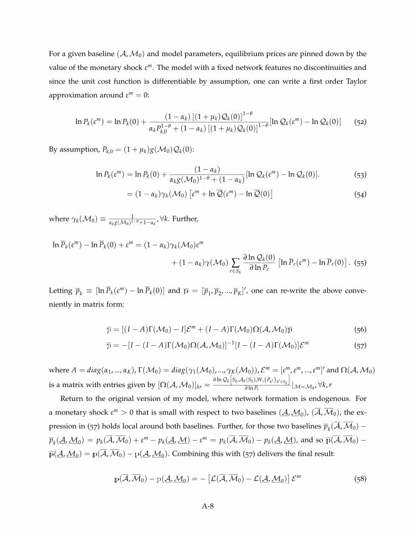
For a given baseline (A,M0) and model parameters, equilibrium prices are pinned down by the

value of the monetary shock εm. The model with a fixed network features no discontinuities and

since the unit cost function is differentiable by assumption, one can write a first order Taylor

approximation around εm = 0:

ln Pk(εm) = ln Pk(0) +

(1− αk) [(1 + µk)Qk(0)]1−θ

αkP1−θk,0 + (1− αk) [(1 + µk)Qk(0)]

1−θ[lnQk(ε

m)− lnQk(0)] (52)

By assumption, Pk,0 = (1 + µk)g(M0)Qk(0):

ln Pk(εm) = ln Pk(0) +

(1− αk)

αkg(M0)1−θ + (1− αk)[lnQk(ε

m)− lnQk(0)]. (53)

= (1− αk)γk(M0)[εm + lnQ(εm)− lnQ(0)

](54)

where γk(M0) ≡ 1αk g(M0)1−θ+1−αk

, ∀k. Further,

ln Pk(εm)− ln Pk(0) + εm = (1− αk)γk(M0)ε

m

+ (1− αk)γ(M0) ∑r∈Sk

∂ lnQk(0)∂ ln Pr

[ln Pr(ε

m)− ln Pr(0)]

. (55)

Letting pk ≡ [ln Pk(εm) − ln Pk(0)] and p = [p1, p2, ..., pK]

′, one can re-write the above conve-

niently in matrix form:

p = [(I − A)Γ(M0)− I]Em + (I − A)Γ(M0)Ω(A,M0)p (56)

p = −[I − (I − A)Γ(M0)Ω(A,M0)]−1[I − (I − A)Γ(M0)]Em (57)

where A = diag(α1, ..., αK), Γ(M0) = diag(γ1(M0), ..., γK(M0)), Em = [εm, εm, ..., εm]′ and Ω(A,M0)

is a matrix with entries given by [Ω(A,M0)]kr =∂ lnQk

[Sk ,Ak(Sk),W,Pk′k′∈Sk

]∂ ln Pr

|M=M0 , ∀k, r

Return to the original version of my model, where network formation is endogenous. For

a monetary shock εm > 0 that is small with respect to two baselines (A,M0), (A,M0), the ex-

pression in (57) holds local around both baselines. Further, for those two baselines pk(A,M0)−

pk(A,M0) = pk(A,M0) + εm − pk(A,M)− εm = pk(A,M0)− pk(A,M), and so p(A,M0)−

p(A,M0) = p(A,M0)− p(A,M0). Combining this with (57) delivers the final result:

p(A,M0)− p(A,M0) = −[L(A,M0)−L(A,M0)

]Em (58)

A-8

where L(A,M0) = [I − (I − A)Γ(M0)Ω(A,M0)]−1 [I − (I − A)Γ(M0)].

Proposition 2. Suppose Assumptions 2-5, 7-8 hold. Consider any two baseline pairs (A,M0), (A,M0)

such that either A ≥ A,M0 =M0 or A = A,M0 ≥ M0. For a monetary shock εm > 0 that is small

with respect to both baselines, it follows that pk(A,M0) ≤ pk(A,M0) for all k = 1, 2, ..., K.

Proof. Let D ≡ Ω(A,M0)−Ω(A,M0), then one can rewrite the difference between the Leontief

Inverses as follows:

L(A,M0)−L(A,M0) =(I − A)Γ(M0)Ω(A,M0)L(A,M0)

− (I − A)Γ(M0)Ω(A,M0)L(A,M0)

− (I − A)Γ(M0)DL(A,M0)

+ (I − A)(Γ(M0)− Γ(M0)). (59)

Let Ξ ≡ diag(

γ1(M0)γ1(M0)

, ..., γK(M0)γK(M0)

), then the above can be re-written as:

L(A,M0)−L(A,M0) = −[I − (I − A)Γ(M0)Ω(A,M0)]−1×

× [(I − A)Γ(M0)DL(A,M0) + (I − A)(I − Ξ)Γ(M0)(I −Ω(A,M0)L(A,M0))]. (60)

From the definition of L(A,M0):

L(A,M0) = [I − (I − A)Γ(M)Ω(A,M0)]−1[I − (I − A)Γ(M0)] =

I + [I − (I − A)Γ(M)Ω(A,M0)]−1(I − A)Γ(M0)(Ω(A,M0)− I)

⇒ I −Ω(A,M0)L(A,M0) = [I −Ω(A,M0)]+

Ω(A,M0)[I − (I − A)Γ(M0)Ω(A,M0)]−1(I − A)Γ(M0)(I −Ω(A,M0)).

(61)

Suppose we have any two baselines pairs (A,M0), (A,M0) such that either A ≥ A,M0 =

M0 or A = A,M0 ≥ M0. Under Cobb-Douglas production function entries of the Ω matrix in

the Leontief Inverse are given by shares in the production function, so that [Ω]kr = ωkr if sector k

buys inputs from sector r and [Ω]kr = 0 otherwise. As a result, D = Ω(A,M0)−Ω(A,M0) is a

K× K matrix with non-negative entries, since from Lemma 2 the first baseline will have (weakly)

A-9

more suppliers for every sector. Further, from the properties of γk, it follows that all entries of

the Ξ matrix are positive and less than or equal to one. Finally, since labor is an essential input,

it follows that sum of rows of (I −Ω(A,M)) for any baseline pair are positive and less than or

equal to one.

Combining the above observations with the expressions in (60) and (61), it follows that for any

two baselines pairs (A,M0), (A,M0) such that either A ≥ A,M0 =M0 or A = A,M0 ≥ M0,

and a monetary shock εm > 0 that is small with respect to both baselines, it holds that:

p(A,M0)− p(A,M0) = −[L(A,M0)−L(A,M0)

]Em ≤ 0K×1. (62)

or pk(A,M0) ≤ pk(A,M0), ∀k in scalar form.

Theorem 1 (Cycle dependence). Suppose Assumptions 3-5, 7-9 hold. For any baseline pair (A,M0),

let ck(A,M0) ≡ ln Ck(A,M)− ln Ck(A,M0), ∀k. Consider any two baseline pairs (A,M0), (A,M0)

such that A ≥ A. For a monetary shock εm > 0 which is small with respect to both baselines it follows

that ck(A,M0) ≥ ck(A,M0) for all k = 1, 2, ..., K, and c(A,M0) ≥ c(A,M0).

Proof. Under Cobb-Douglas aggregation of sectoral consumption it follows that sectoral con-

sumption demand takes the following form:

Ck = ωck

[Pk

Pc

]−1

C = ωckPcCPk

= ωckMPk

. (63)

From the above it follows that ln Ck = ln ωck + lnM− ln Pk and evaluating the latter under

baseline and following the shock yields:

ln Ck(A,M)− ln Ck(A,M0) = lnM− ln Pk(A,M)− lnM0 + ln Pk(A,M0)

ck(A,M0) = εm − pk(A,M0). (64)

For the two baselines (A,M0), (A,M0) such that A ≥ A, and a monetary shock εm > 0 that is

small with respect to both baselines it follows:

ck(A,M0)− ck(A,M0) = −[pk(A,M0)− pk(A,M0)

]≥ 0, ∀k (65)

where the last part follows from Proposition 2.

A-10

Consider deviation of aggregate consumption from baseline:

ck(A,M0)− ck(A,M0) =K

∑k=1

ωck[ck(A,M0)− ck(A,M0)

]≥ 0. (66)

Theorem 2 (Path dependence). Suppose Assumptions 3-5, 7-9 hold. For any baseline pair (A,M0), let

ck(A,M0) ≡ ln Ck(A,M)− ln Ck(A,M0), ∀k. Consider any two baseline pairs (A,M0), (A,M0)

such thatM0 ≥M0. For a monetary shock εm > 0 which is small with respect to both baselines it follows

that ck(A,M0) ≥ ck(A,M0) for all k = 1, 2, ..., K, and c(A,M0) ≥ c(A,M0).

Proof. Recall from the proof of Theorem 1 it is true that ck(A,M0) = εm − pk(A,M0), ∀k. For

the two baselines (A,M0), (A,M0) such that M0 ≥ M0, and a monetary shock εm > 0 that is

small with respect to both baselines it follows:

ck(A,M0)− ck(A,M0) = −[pk(A,M0)− pk(A,M0)

]≥ 0 (67)

where the last part follows from Proposition 2.

Consider deviation of aggregate consumption from baseline:

ck(A,M0)− ck(A,M0) =K

∑k=1

ωck[ck(A,M0)− ck(A,M0)

]≥ 0. (68)

Proposition 3. Suppose Assumption 1-5 hold. For a baseline pair (A,M0), let εm > 0 be a small

monetary shock and Em > 0 be a large monetary shock. Under the large monetary shock, the equilibrium

set of supplier choices is SLk ⊃ Sk(A,M0) = S0

k , ∀k. The ratios of exact impulse responses of sectoral

prices satisfy:Pe

k (Em; SL)

Pek (ε

m; SL)≤ Pk(Em)

Pk(εm)≤ Pe(Em; S0)

Pek (ε

m; S0), (69)

for all k = 1, 2, ..., K.

Proof. Starting from a baseline pair (A,M0), following the large monetary shock the original

A-11

network S0 is still available, but is not chosen, hence:

Qk(SLk ,Ak(SL

k ),ML, Pk(ML, SL)Kr=1) ≤ Qk(S0

k ,Ak(S0k),ML, Pk(ML, S0)K

r=1) (70)

⇒ Pk(SLk ,ML) ≤ Pk(S0

k ,ML) (71)

⇒Pk(SL

k ,ML)

Pk(S0k ,M0)

≤Pk(S0

k ,ML)

Pk(S0k ,M0)

(72)

⇒ Pk(Em) ≤ Pek (Em; S0) (73)

⇒ Pk(Em)

Pk(εm)≤

Pek (Em; S0)

Pek (ε

m; S0)(74)

Starting from a baseline pair (A,M0), following the small monetary shock the network SL is

available, but is not chosen, hence:

Qk(S0k ,Ak(S0

k),M∫ , Pk(M∫ , S0)Kr=1) ≤ Qk(SL

k ,Ak(SLk ),M∫ , Pk(M∫ , SL)K

r=1) (75)

⇒ Pk(S0k ,Ms) ≤ Pk(SL

k ,Ms) (76)

⇒ 1Pk(S0

k ,Ms)≥ 1

Pk(SLk ,Ms)

(77)

⇒Pk(SL

k ,ML)

Pk(S0k ,Ms)

≥Pk(SL

k ,ML)

Pk(SLk ,Ms)

(78)

⇒Pk(SL

k ,ML)/Pk(S0k ,M0)

Pk(S0k ,Ms)/Pk(S0

k ,M0)≥

Pk(SLk ,ML)//Pk(SL

k ,M0)

Pk(SLk ,Ms)/Pk(SL

k ,M0)(79)

⇒ Pk(Em)

Pk(εm)≥

Pek (Em; SL)

Pek (ε

m; SL)(80)

Combining (74) and (80):Pe

k (Em; SL)

Pek (ε

m; SL)≤ Pk(Em)

Pk(εm)≤ Pe(Em; S0)

Pek (ε

m; S0), (81)

for all k = 1, 2, ..., K.

Theorem 3 (Size dependence). Suppose Assumption 1-5 hold. For a baseline pair (A,M0), let εm > 0

be a small monetary shock and Em > 0 be a large monetary shock. Under the large monetary shock, the

equilibrium set of supplier choices is SLk ⊃ Sk(A,M0) = S0

k , ∀k. The ratios of exact impulse responses of

GDP satisfy:Ce(Em; S0)

Ce(εm; S0)≤ C(Em)

C(εm)≤ Ce(Em; SL)

Ce(εm; SL). (82)

Proof. Recall from (71) that Pk(SLk ,ML) ≤ Pk(S0

k ,ML)∀k, which implies that Pk(SLk ,ML) ≤

A-12

Pk(S0k ,ML)∀k. Hence,

Pc(SL,ML) = Pc(P1(SL

1 ,ML), ..., PK(SLK,ML)) ≤ Pc(P1(S0

1,ML), ..., PK(S0K,ML)) = Pc

(S0,ML).

(83)

From the cash-in-advance constraint. combined with (83):

C(SL,ML)

C(S0,ML)=

Pc(S0,ML)

Pc(SL,ML)

≥ 1 (84)

⇒ C(SL,ML) ≥ C(S0,ML) (85)

⇒ C(SL,ML)

C(S0,Ms)≥ C(S0,ML)

C(S0,Ms)(86)

⇒ C(SL,ML)/C(S0,M0)

C(S0,Ms)/C(S0,M0)≥ C(S0,ML)/C(S0,M0)

C(S0,Ms)/C(S0,M0)(87)

⇒ C(Em)

C(εm)≥ Ce(Em; S0)

Ce(εm; S0). (88)

Recall from (76) that Pk(S0k ,Ms) ≤ Pk(SL

k ,Ms)∀k, which implies that Pk(S0k ,Ms) ≤ Pk(SL

k ,Ms)∀k.

Hence,

Pc(S0,Ms) = Pc(P1(S0

1,Ms), ..., PK(S0K,Ms)) ≤ Pc(P1(SL

1 ,Ms), ..., PK(SLK,Ms)) = Pc

(SL,Ms).

(89)

From the cash-in-advance constraint. combined with (89):

C(S0,Ms)

C(SL,Ms)=

Pc(Sl ,Ms)

Pc(S0,Ms)

≥ 1 (90)

⇒ 1C(S0,Ms)

≤ 1C(SL,Ms)

(91)

⇒ C(SL,ML)

C(S0,Ms)≤ C(SL,ML)

C(SL,Ms)(92)

⇒ C(SL,ML)/C(S0,M0)

C(S0,Ms)/C(S0,M0)≤ C(SL,ML)/C(SL,M0)

C(SL,Ms)/C(SL,M0)(93)

⇒ C(Em)

C(εm)≤ Ce(Em; SL)

Ce(εm; SL). (94)

Combine (88) and (94): Ce(Em; S0)

Ce(εm; S0)≤ C(Em)

C(εm)≤ Ce(Em; SL)

Ce(εm; SL). (95)

A-13

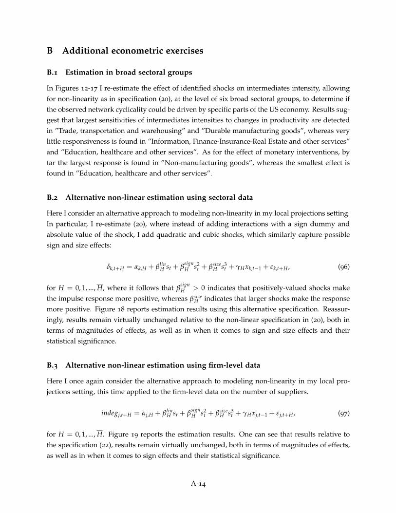
B Additional econometric exercises

B.1 Estimation in broad sectoral groups

In Figures 12-17 I re-estimate the effect of identified shocks on intermediates intensity, allowingfor non-linearity as in specification (20), at the level of six broad sectoral groups, to determine ifthe observed network cyclicality could be driven by specific parts of the US economy. Results sug-gest that largest sensitivities of intermediates intensities to changes in productivity are detectedin ”Trade, transportation and warehousing” and ”Durable manufacturing goods”, whereas verylittle responsiveness is found in ”Information, Finance-Insurance-Real Estate and other services”and ”Education, healthcare and other services”. As for the effect of monetary interventions, byfar the largest response is found in ”Non-manufacturing goods”, whereas the smallest effect isfound in ”Education, healthcare and other services”.

B.2 Alternative non-linear estimation using sectoral data

Here I consider an alternative approach to modeling non-linearity in my local projections setting.In particular, I re-estimate (20), where instead of adding interactions with a sign dummy andabsolute value of the shock, I add quadratic and cubic shocks, which similarly capture possiblesign and size effects:

δk,t+H = αk,H + βlinH st + β

signH s2

t + βsizeH s3

t + γHxk,t−1 + εk,t+H, (96)

for H = 0, 1, ..., H, where it follows that βsignH > 0 indicates that positively-valued shocks make

the impulse response more positive, whereas βsizeH indicates that larger shocks make the response

more positive. Figure 18 reports estimation results using this alternative specification. Reassur-ingly, results remain virtually unchanged relative to the non-linear specification in (20), both interms of magnitudes of effects, as well as in when it comes to sign and size effects and theirstatistical significance.

B.3 Alternative non-linear estimation using firm-level data

Here I once again consider the alternative approach to modeling non-linearity in my local pro-jections setting, this time applied to the firm-level data on the number of suppliers.

indegj,t+H = αj,H + βlinH st + β

signH s2

t + βsizeH s3

t + γHxj,t−1 + ε j,t+H, (97)

for H = 0, 1, ..., H. Figure 19 reports the estimation results. One can see that results relative tothe specification (22), results remain virtually unchanged, both in terms of magnitudes of effects,as well as in when it comes to sign effects and their statistical significance.

A-14

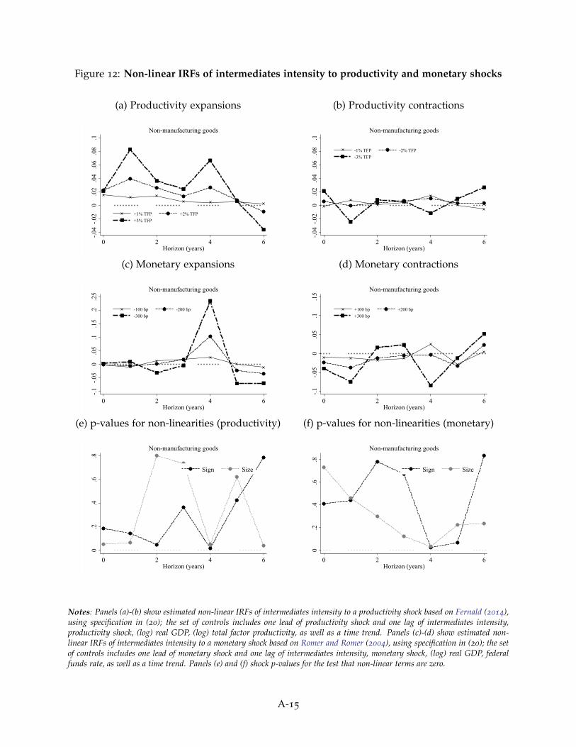
Figure 12: Non-linear IRFs of intermediates intensity to productivity and monetary shocks

(a) Productivity expansions-.0

4-.0

20

.02

.04

.06

.08

.1

0 2 4 6Horizon (years)

+1% TFP +2% TFP+3% TFP

Non-manufacturing goods

(b) Productivity contractions

-.04

-.02

0.0

2.0

4.0

6.0

8.1

0 2 4 6Horizon (years)

-1% TFP -2% TFP-3% TFP

Non-manufacturing goods

(c) Monetary expansions

-.1-.0

50

.05

.1.1

5.2

.25

0 2 4 6Horizon (years)

-100 bp -200 bp-300 bp

Non-manufacturing goods

(d) Monetary contractions

-.1-.0

50

.05

.1.1

5

0 2 4 6Horizon (years)

+100 bp +200 bp+300 bp

Non-manufacturing goods

(e) p-values for non-linearities (productivity)

0.2

.4.6

.8

0 2 4 6Horizon (years)

Sign Size

Non-manufacturing goods

(f) p-values for non-linearities (monetary)

0.2

.4.6

.8

0 2 4 6Horizon (years)

Sign Size

Non-manufacturing goods

Notes: Panels (a)-(b) show estimated non-linear IRFs of intermediates intensity to a productivity shock based on Fernald (2014),using specification in (20); the set of controls includes one lead of productivity shock and one lag of intermediates intensity,productivity shock, (log) real GDP, (log) total factor productivity, as well as a time trend. Panels (c)-(d) show estimated non-linear IRFs of intermediates intensity to a monetary shock based on Romer and Romer (2004), using specification in (20); the setof controls includes one lead of monetary shock and one lag of intermediates intensity, monetary shock, (log) real GDP, federalfunds rate, as well as a time trend. Panels (e) and (f) shock p-values for the test that non-linear terms are zero.

A-15

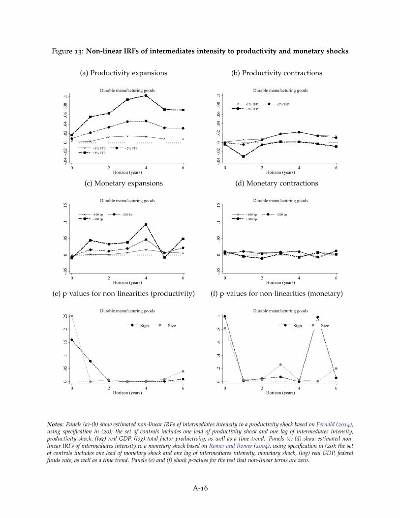
Figure 13: Non-linear IRFs of intermediates intensity to productivity and monetary shocks

(a) Productivity expansions-.0

4-.0

20

.02

.04

.06

.08

.1

0 2 4 6Horizon (years)

+1% TFP +2% TFP+3% TFP

Durable manufacturing goods

(b) Productivity contractions

-.04

-.02

0.0

2.0

4.0

6.0

8.1

0 2 4 6Horizon (years)

-1% TFP -2% TFP-3% TFP

Durable manufacturing goods

(c) Monetary expansions

-.05

0.0

5.1

.15

0 2 4 6Horizon (years)

-100 bp -200 bp-300 bp

Durable manufacturing goods

(d) Monetary contractions

-.05

0.0

5.1

.15

0 2 4 6Horizon (years)

+100 bp +200 bp+300 bp

Durable manufacturing goods

(e) p-values for non-linearities (productivity)

0.0

5.1

.15

.2.2

5

0 2 4 6Horizon (years)

Sign Size

Durable manufacturing goods

(f) p-values for non-linearities (monetary)

0.2

.4.6

.81

0 2 4 6Horizon (years)

Sign Size

Durable manufacturing goods

Notes: Panels (a)-(b) show estimated non-linear IRFs of intermediates intensity to a productivity shock based on Fernald (2014),using specification in (20); the set of controls includes one lead of productivity shock and one lag of intermediates intensity,productivity shock, (log) real GDP, (log) total factor productivity, as well as a time trend. Panels (c)-(d) show estimated non-linear IRFs of intermediates intensity to a monetary shock based on Romer and Romer (2004), using specification in (20); the setof controls includes one lead of monetary shock and one lag of intermediates intensity, monetary shock, (log) real GDP, federalfunds rate, as well as a time trend. Panels (e) and (f) shock p-values for the test that non-linear terms are zero.

A-16

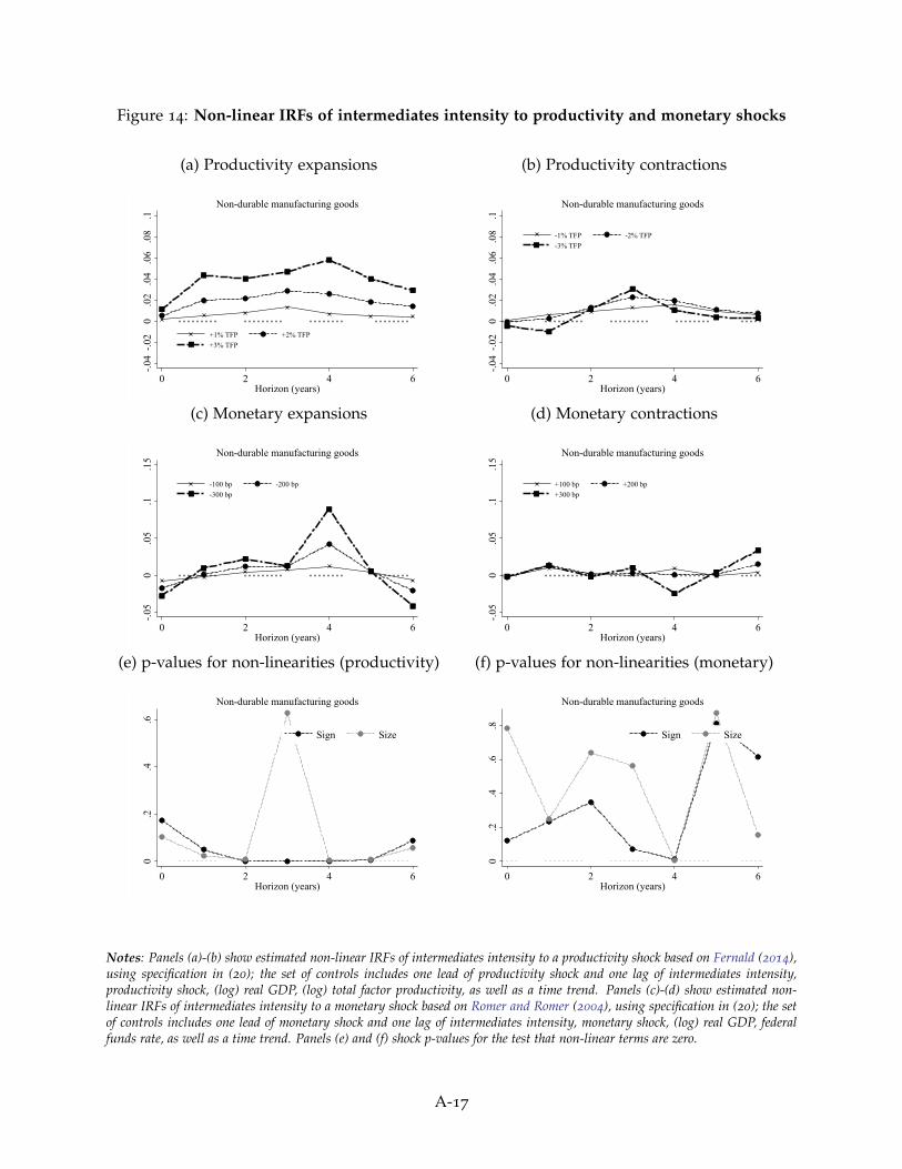
Figure 14: Non-linear IRFs of intermediates intensity to productivity and monetary shocks

(a) Productivity expansions-.0

4-.0

20

.02

.04

.06

.08

.1

0 2 4 6Horizon (years)

+1% TFP +2% TFP+3% TFP

Non-durable manufacturing goods

(b) Productivity contractions

-.04

-.02

0.0

2.0

4.0

6.0

8.1

0 2 4 6Horizon (years)

-1% TFP -2% TFP-3% TFP

Non-durable manufacturing goods

(c) Monetary expansions

-.05

0.0

5.1

.15

0 2 4 6Horizon (years)

-100 bp -200 bp-300 bp

Non-durable manufacturing goods

(d) Monetary contractions

-.05

0.0

5.1

.15

0 2 4 6Horizon (years)

+100 bp +200 bp+300 bp

Non-durable manufacturing goods

(e) p-values for non-linearities (productivity)

0.2

.4.6

0 2 4 6Horizon (years)

Sign Size

Non-durable manufacturing goods

(f) p-values for non-linearities (monetary)

0.2

.4.6

.8

0 2 4 6Horizon (years)

Sign Size

Non-durable manufacturing goods

Notes: Panels (a)-(b) show estimated non-linear IRFs of intermediates intensity to a productivity shock based on Fernald (2014),using specification in (20); the set of controls includes one lead of productivity shock and one lag of intermediates intensity,productivity shock, (log) real GDP, (log) total factor productivity, as well as a time trend. Panels (c)-(d) show estimated non-linear IRFs of intermediates intensity to a monetary shock based on Romer and Romer (2004), using specification in (20); the setof controls includes one lead of monetary shock and one lag of intermediates intensity, monetary shock, (log) real GDP, federalfunds rate, as well as a time trend. Panels (e) and (f) shock p-values for the test that non-linear terms are zero.

A-17

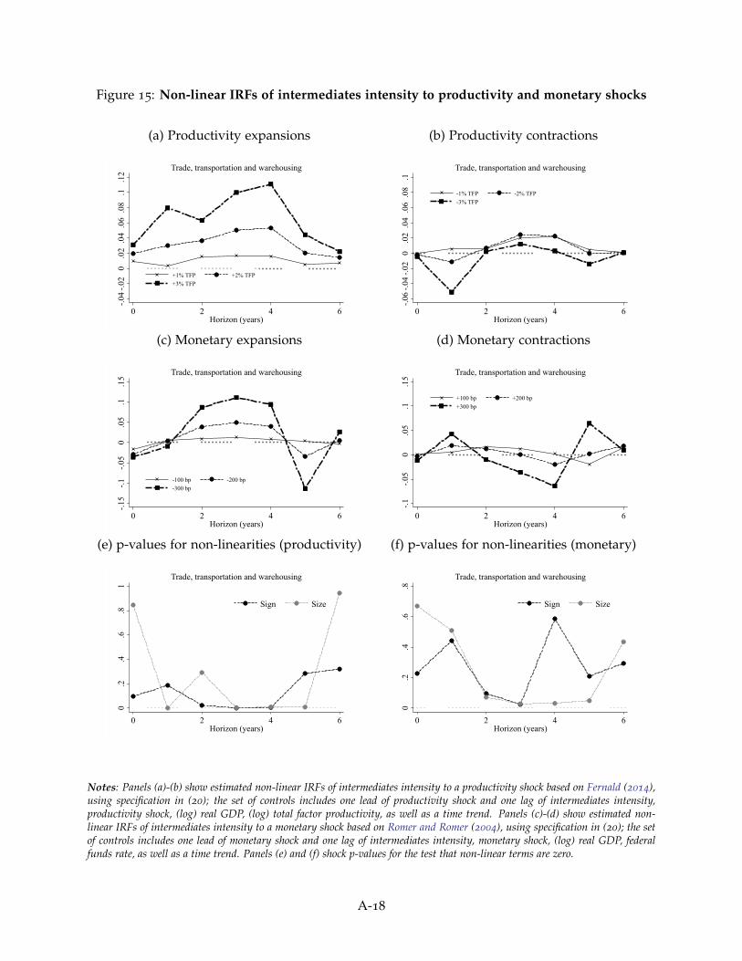
Figure 15: Non-linear IRFs of intermediates intensity to productivity and monetary shocks

(a) Productivity expansions-.0

4-.0

20

.02

.04

.06

.08

.1.1

2

0 2 4 6Horizon (years)

+1% TFP +2% TFP+3% TFP

Trade, transportation and warehousing

(b) Productivity contractions

-.06

-.04

-.02

0.0

2.0

4.0

6.0

8.1

0 2 4 6Horizon (years)

-1% TFP -2% TFP-3% TFP

Trade, transportation and warehousing

(c) Monetary expansions

-.15

-.1-.0

50

.05

.1.1

5

0 2 4 6Horizon (years)

-100 bp -200 bp-300 bp

Trade, transportation and warehousing

(d) Monetary contractions

-.1-.0

50

.05

.1.1

5

0 2 4 6Horizon (years)

+100 bp +200 bp+300 bp

Trade, transportation and warehousing

(e) p-values for non-linearities (productivity)

0.2

.4.6

.81

0 2 4 6Horizon (years)

Sign Size

Trade, transportation and warehousing

(f) p-values for non-linearities (monetary)

0.2

.4.6

.8

0 2 4 6Horizon (years)

Sign Size

Trade, transportation and warehousing

Notes: Panels (a)-(b) show estimated non-linear IRFs of intermediates intensity to a productivity shock based on Fernald (2014),using specification in (20); the set of controls includes one lead of productivity shock and one lag of intermediates intensity,productivity shock, (log) real GDP, (log) total factor productivity, as well as a time trend. Panels (c)-(d) show estimated non-linear IRFs of intermediates intensity to a monetary shock based on Romer and Romer (2004), using specification in (20); the setof controls includes one lead of monetary shock and one lag of intermediates intensity, monetary shock, (log) real GDP, federalfunds rate, as well as a time trend. Panels (e) and (f) shock p-values for the test that non-linear terms are zero.

A-18

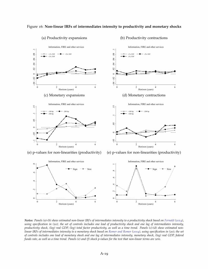
Figure 16: Non-linear IRFs of intermediates intensity to productivity and monetary shocks

(a) Productivity expansions-.0

4-.0

20

.02

.04

.06

.08

.1

0 2 4 6Horizon (years)

+1% TFP +2% TFP+3% TFP

Information, FIRE and other services

(b) Productivity contractions

-.04

-.02

0.0

2.0

4.0

6.0

8.1

0 2 4 6Horizon (years)

-1% TFP -2% TFP-3% TFP

Information, FIRE and other services

(c) Monetary expansions

-.1-.0

50

.05

.1.1

5

0 2 4 6Horizon (years)

-100 bp -200 bp-300 bp

Information, FIRE and other services

(d) Monetary contractions

-.05

0.0

5.1

.15

0 2 4 6Horizon (years)

+100 bp +200 bp+300 bp

Information, FIRE and other services

(e) p-values for non-linearities (productivity)

0.2

.4.6

.8

0 2 4 6Horizon (years)

Sign Size

Information, FIRE and other services

(e) p-values for non-linearities (productivity)

0.2

.4.6

.81

0 2 4 6Horizon (years)

Sign Size

Information, FIRE and other services

Notes: Panels (a)-(b) show estimated non-linear IRFs of intermediates intensity to a productivity shock based on Fernald (2014),using specification in (20); the set of controls includes one lead of productivity shock and one lag of intermediates intensity,productivity shock, (log) real GDP, (log) total factor productivity, as well as a time trend. Panels (c)-(d) show estimated non-linear IRFs of intermediates intensity to a monetary shock based on Romer and Romer (2004), using specification in (20); the setof controls includes one lead of monetary shock and one lag of intermediates intensity, monetary shock, (log) real GDP, federalfunds rate, as well as a time trend. Panels (e) and (f) shock p-values for the test that non-linear terms are zero.

A-19

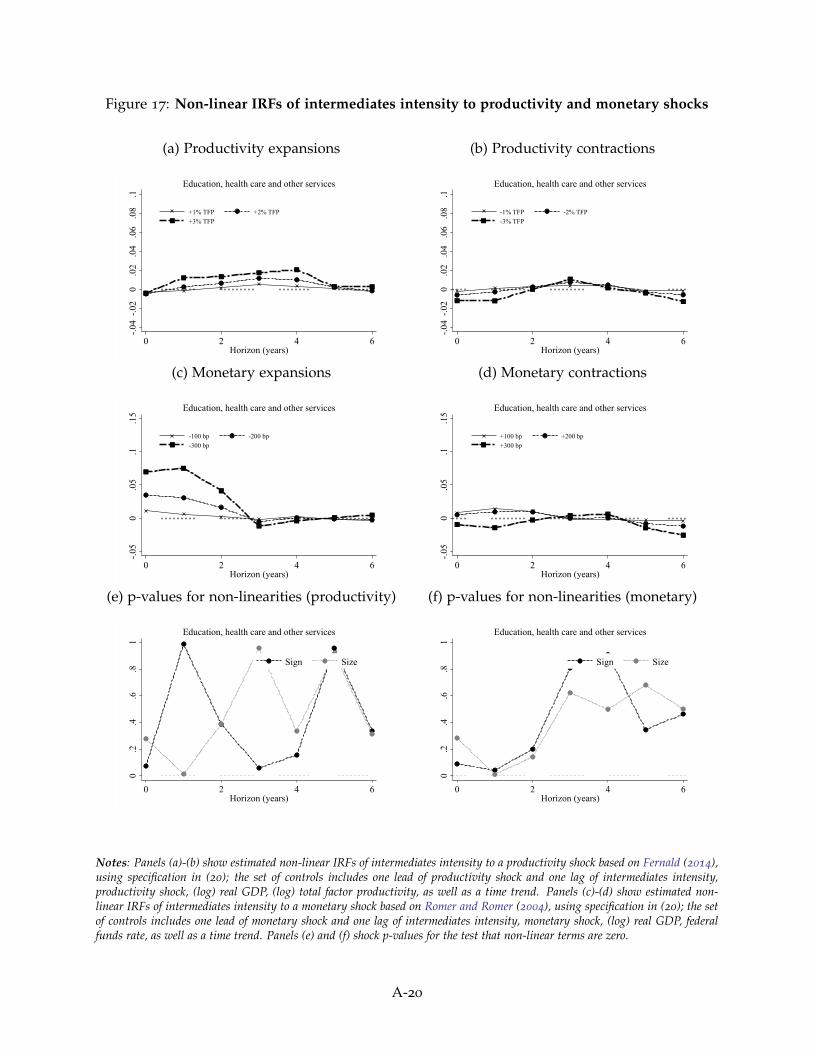
Figure 17: Non-linear IRFs of intermediates intensity to productivity and monetary shocks

(a) Productivity expansions-.0

4-.0

20

.02

.04

.06

.08

.1

0 2 4 6Horizon (years)

+1% TFP +2% TFP+3% TFP

Education, health care and other services

(b) Productivity contractions

-.04

-.02

0.0

2.0

4.0

6.0

8.1

0 2 4 6Horizon (years)

-1% TFP -2% TFP-3% TFP

Education, health care and other services

(c) Monetary expansions

-.05

0.0

5.1

.15

0 2 4 6Horizon (years)

-100 bp -200 bp-300 bp

Education, health care and other services

(d) Monetary contractions

-.05

0.0

5.1

.15

0 2 4 6Horizon (years)

+100 bp +200 bp+300 bp

Education, health care and other services

(e) p-values for non-linearities (productivity)

0.2

.4.6

.81

0 2 4 6Horizon (years)

Sign Size

Education, health care and other services

(f) p-values for non-linearities (monetary)

0.2

.4.6

.81

0 2 4 6Horizon (years)

Sign Size

Education, health care and other services

Notes: Panels (a)-(b) show estimated non-linear IRFs of intermediates intensity to a productivity shock based on Fernald (2014),using specification in (20); the set of controls includes one lead of productivity shock and one lag of intermediates intensity,productivity shock, (log) real GDP, (log) total factor productivity, as well as a time trend. Panels (c)-(d) show estimated non-linear IRFs of intermediates intensity to a monetary shock based on Romer and Romer (2004), using specification in (20); the setof controls includes one lead of monetary shock and one lag of intermediates intensity, monetary shock, (log) real GDP, federalfunds rate, as well as a time trend. Panels (e) and (f) shock p-values for the test that non-linear terms are zero.

A-20

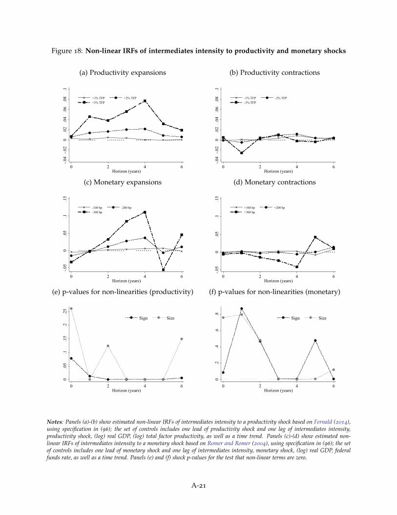
Figure 18: Non-linear IRFs of intermediates intensity to productivity and monetary shocks

(a) Productivity expansions-.0

4-.0

20

.02

.04

.06

.08

.1

0 2 4 6Horizon (years)

+1% TFP +2% TFP+3% TFP

(b) Productivity contractions

-.04

-.02

0.0

2.0

4.0

6.0

8.1

0 2 4 6Horizon (years)

-1% TFP -2% TFP-3% TFP

(c) Monetary expansions

-.05

0.0

5.1

.15

0 2 4 6Horizon (years)

-100 bp -200 bp-300 bp

(d) Monetary contractions

-.05

0.0

5.1

.15

0 2 4 6Horizon (years)

+100 bp +200 bp+300 bp

(e) p-values for non-linearities (productivity)

0.0

5.1

.15

.2.2

5

0 2 4 6Horizon (years)

Sign Size

(f) p-values for non-linearities (monetary)

0.2

.4.6

.8

0 2 4 6Horizon (years)

Sign Size

Notes: Panels (a)-(b) show estimated non-linear IRFs of intermediates intensity to a productivity shock based on Fernald (2014),using specification in (96); the set of controls includes one lead of productivity shock and one lag of intermediates intensity,productivity shock, (log) real GDP, (log) total factor productivity, as well as a time trend. Panels (c)-(d) show estimated non-linear IRFs of intermediates intensity to a monetary shock based on Romer and Romer (2004), using specification in (96); the setof controls includes one lead of monetary shock and one lag of intermediates intensity, monetary shock, (log) real GDP, federalfunds rate, as well as a time trend. Panels (e) and (f) shock p-values for the test that non-linear terms are zero.

A-21

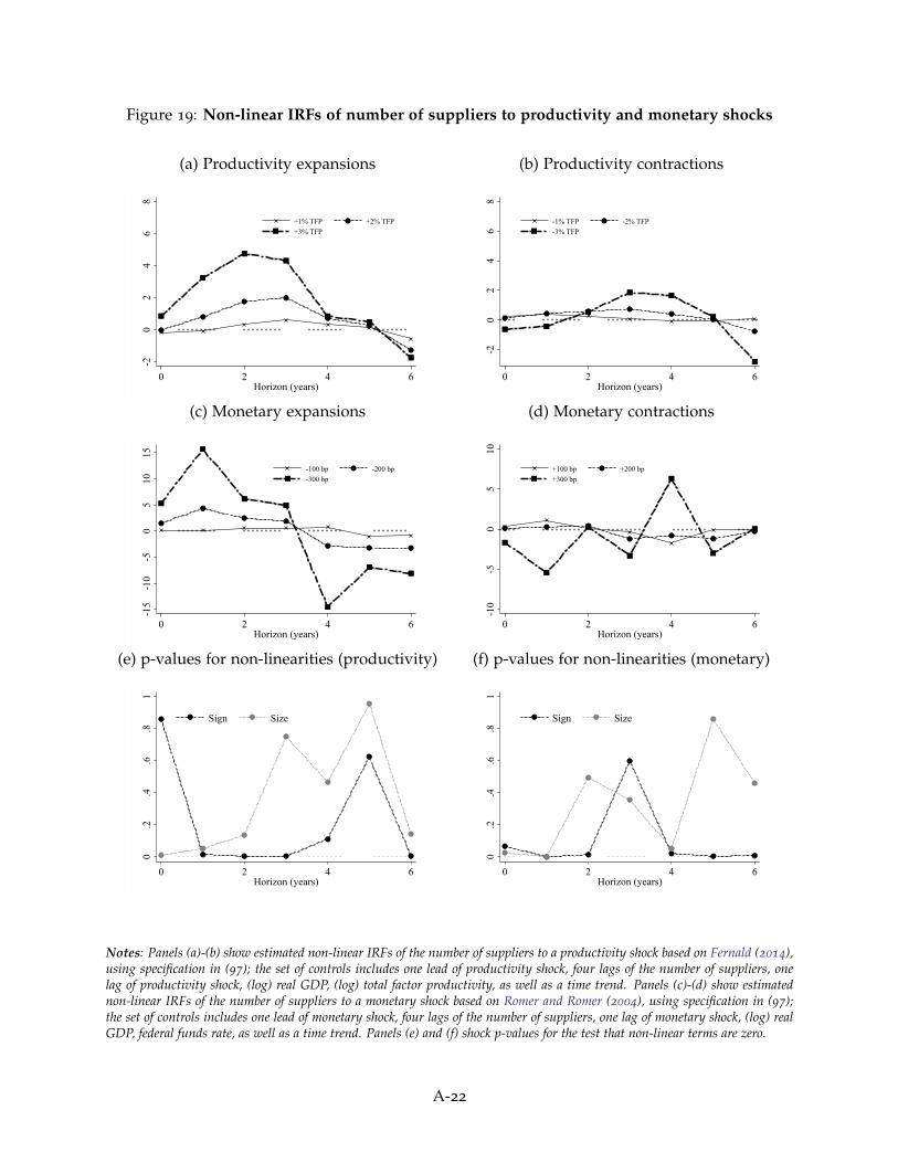
Figure 19: Non-linear IRFs of number of suppliers to productivity and monetary shocks

(a) Productivity expansions-2

02

46

8

0 2 4 6Horizon (years)

+1% TFP +2% TFP+3% TFP

(b) Productivity contractions

-20

24

68

0 2 4 6Horizon (years)

-1% TFP -2% TFP-3% TFP

(c) Monetary expansions

-15

-10

-50

510

15

0 2 4 6Horizon (years)

-100 bp -200 bp-300 bp

(d) Monetary contractions

-10

-50

510

0 2 4 6Horizon (years)

+100 bp +200 bp+300 bp

(e) p-values for non-linearities (productivity)

0.2

.4.6

.81

0 2 4 6Horizon (years)

Sign Size

(f) p-values for non-linearities (monetary)

0.2

.4.6

.81

0 2 4 6Horizon (years)

Sign Size

Notes: Panels (a)-(b) show estimated non-linear IRFs of the number of suppliers to a productivity shock based on Fernald (2014),using specification in (97); the set of controls includes one lead of productivity shock, four lags of the number of suppliers, onelag of productivity shock, (log) real GDP, (log) total factor productivity, as well as a time trend. Panels (c)-(d) show estimatednon-linear IRFs of the number of suppliers to a monetary shock based on Romer and Romer (2004), using specification in (97);the set of controls includes one lead of monetary shock, four lags of the number of suppliers, one lag of monetary shock, (log) realGDP, federal funds rate, as well as a time trend. Panels (e) and (f) shock p-values for the test that non-linear terms are zero.

A-22